The 6.1.4, 6.0.18, and 4.9.337
stable kernel updates have been released; each contains another set of
important fixes.
Greg Kroah-Hartman has also let it be known
that 4.9.337 is the end of the line for the 4.9 kernel, which was released
just over six years ago. “This kernel is now END-OF-LIFE and you should move to 4.14.y at the
least, 6.1.y is the better option.”
I have a patchset that makes it safe to use hibernation under Linux even in a secure boot world but it relies on preventing userland from using one of the TPM PCRs[1] that would otherwise be available to it. TPM 2 devices support emulating PCRs in NVRAM, which would obviously be beneficial in not taking away a scare resource, but the docs suggest there’s no way to tie a key generation to an NVRAM value which makes this more complicated.
So, why not ask a computer to do this for me? I asked ChatGPT to write me some code that would bind a TPM key to an NVRAM value. After a couple of false starts it told me:To bind an encryption key to the value of a TPM NV index, you can use the TPM2_NV_DefineSpace command to define an NV index with the TPMA_NV_BIND attribute. Woo! That sounds perfect. Only one problem – I can’t actually find the TPMA_NV_BIND attribute defined anywhere in the spec. Well, ask the AI again.
Here is the definition of TPMA_NV_BIND from the TPM 2.0 specification: TPMA_NV_BIND (BIT 17) If SET, the contents of the NV Index are bound to the platform hierarchy.
Ok, that sounds convincing. Where is it in the spec?
The definition of TPMA_NV_BIND is on page 126 of the TPM 2.0 specification, in section 9.7.1 “TPMA_NV”.
Huh. Nope. Page 126 says nothing about this. Section 9.7.1 says nothing about this. The TPMA_NV bits are actually described on page 168 of volume 2 of the spec, in section 13.4. Bit 17 is TPMA_NV_OWNERREAD. TPMA_NV_BIND does not appear in the spec anywhere. I told the AI that.
I apologize for the error in my previous response. You are correct that the TPMA_NV_BIND attribute does not appear in the TPM 2.0 specification.
To bind an encryption key to the value of a TPM NV index, you can use the TPM2_NV_DefineSpace command with the TPMA_NV_BIND attribute.
I’m not afraid of being unemployed in the near future.
[1] “Platform Configuration Registers” – a modern TPM has 24 of these. When something security sensitive happens, you generate a hash of that event and pass it to the TPM. The TPM appends that to an existing PCR value and then hashes that concatenated value and sets the PCR to that. This means the PCR value depends not only on the values provided, but also the order they’re provided in. Various TPM operations can be made conditional on the PCR values meeting specific criteria.
In this post, we demonstrate how to build a simple web-based search application using the recently announced Amazon OpenSearch Serverless, a serverless option for Amazon OpenSearch Service that makes it easy to run petabyte-scale search and analytics workloads without having to think about clusters. The benefit of using OpenSearch Serverless as a backend for your search application is that it automatically provisions and scales the underlying resources based on the search traffic demands, so you don’t have to worry about infrastructure management. You can simply focus on building your search application and analyzing the results. OpenSearch Serverless is powered by the open-source OpenSearch project, which consists of a search engine, and OpenSearch Dashboards, a visualization tool to analyze your search results.
Solution overview
There are many ways to build a search application. In our example, we create a simple Java script front end and call Amazon API Gateway, which triggers an AWS Lambda function upon receiving user queries. As shown in the following diagram, API Gateway acts as a broker between the front end and the OpenSearch Serverless collection. When the user queries the front-end webpage, API Gateway passes requests to the Python Lambda function, which runs the queries on the OpenSearch Serverless collection and returns the search results.
To get started with the search application, you must first upload the relevant dataset, a movie catalog in this case, to the OpenSearch collection and index them to make them searchable.
After your collection is created and active, you can upload the movie data to an index in this collection. Indexes hold documents, and each document in this example represents a movie record. Documents are comparable to rows in the database table. Each document (the movie record) consists of 10 fields that are typically searched for in a movie catalog, like the director, actor, release date, genre, title, or plot of the movie. The following is a sample movie JSON document:
{
"directors": ["David Yates"],
"release_date": "2011-07-07T00:00:00Z",
"rating": 8.1,
"genres": ["Adventure", "Family", "Fantasy", "Mystery"],
"plot": "Harry, Ron and Hermione search for Voldemort's remaining Horcruxes in their effort to destroy the Dark Lord.",
"title": "Harry Potter and the Deathly Hallows: Part 2",
"rank": 131,
"running_time_secs": 7800,
"actors": ["Daniel Radcliffe", "Emma Watson", "Rupert Grint"],
"year": 2011
}
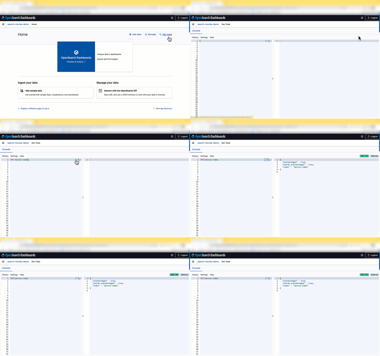
For the search catalog, you can upload the sample-movies.bulk dataset sourced from the Internet Movies Database (IMDb). OpenSearch Serverless offers the same ingestion pipeline and clients to ingest the data as OpenSearch Service, such as Fluentd, Logstash, and Postman. Alternatively, you can use the OpenSearch Dashboards Dev Tools to ingest and search the data without configuring any additional pipelines. To do so, log in to OpenSearch Dashboards using your SAML credentials and choose Dev tools.
To create a new index, use the PUT command followed by the index name:
PUT movies-index
A confirmation message is displayed upon successful creation of your index.
After the index is created, you can ingest documents into the index. OpenSearch provides the option to ingest multiple documents in one request using the _bulk request. Enter POST /_bulk in the left pane as shown in the following screenshot, then copy and paste the contents of the sample-movies.bulk file you downloaded earlier.
You have successfully created the movies index and uploaded 1,500 records into the catalog! Now let’s integrate the movie catalog with your search application.
Integrate the Lambda function with an OpenSearch Serverless endpoint
In this step, you create a Lambda function that queries the movie catalog in OpenSearch Serverless and returns the result. For more information, see our tutorial on creating a Lambda function for connecting to and querying an OpenSearch Service domain. You can reuse the same code by replacing the parameters to align to OpenSearch Serverless’s requirements. Replace <my-region> with your corresponding region (for example, us-west-2), use aoss instead of es for service, replace <hostname> with the OpenSearch collection endpoint, and <index-name> with your index (in this case, movies-index).
The following is a snippet of the Lambda code. You can find the complete code in the tutorial.
import boto3
import json
import requests
from requests_aws4auth import AWS4Auth

region = '<my-region>'
service = 'aoss'
credentials = boto3.Session().get_credentials()
awsauth = AWS4Auth(credentials.access_key, credentials.secret_key, region, service, session_token=credentials.token)

host = '<hostname>'
# The OpenSearch collection endpoint
index = '<index-name>'
url = host + '/' + index + '/_search'

# Lambda execution starts here
def Lambda_handler(event, context):
This Lambda function returns a list of movies based on a search string (such as movie title, director, or actor) provided by the user.
Next, you need to configure the permissions in OpenSearch Serverless’s data access policy to let the Lambda function access the collection.
On the Lambda console, navigate to your function.
On the Configuration tab, in the Permissions section, under Execution role, copy the value for Role name.
Add this role name as one of the principals of your movie-search collection’s data access policy.
Principals can be AWS Identity and Access Management (IAM) users, role ARNs, or SAML identities. These principals must be within the current AWS account.
After you add the role name as a principal, you can see the role ARN updated in your rule, as show in the following screenshot.
Now you can grant collection and index permissions to this principal.
For more details about data access policies, refer to Data access control for Amazon OpenSearch Serverless. Skipping this step or not running it correctly will result in permission errors, and your Lambda code won’t be able to query the movie catalog.
Configure API Gateway
API Gateway acts as a front door for applications to access the code running on Lambda. To create, configure, and deploy the API for the GET method, refer to the steps in the tutorial. For API Gateway to pass the requests to the Lambda function, configure it as a trigger to invoke the Lambda function.
The next step is to integrate it with the front end.
Test the web application
To build the front-end UI, you can download the following sample JavaScript web service. Open the scripts/search.js file and update the apigatewayendpoint variable to point to your API Gateway endpoint:
var apigatewayendpoint = 'https://kxxxxxxzzz.execute-api.us-west-2.amazonaws.com/opensearch-api-test/';
// Update this variable to point to your API Gateway endpoint.
You can access the front-end application by opening index.html in your browser. When the user runs a query on the front-end application, it calls API Gateway and Lambda to serve up the content hosted in the OpenSearch Serverless collection.
When you search the movie catalog, the Lambda function runs the following query:
    # Put the user query into the query DSL for more accurate search results.
    # Note that certain fields are boosted (^).
    query = {
        "size": 25,
        "query": {
            "multi_match": {
                "query": event['queryStringParameters']['q'],
                "fields": ["title", "plot", "actors"]
            }
        }
    }
The query returns documents based on a provided query string. Let’s look at the parameters used in the query:
size – The size parameter is the maximum number of documents to return. In this case, a maximum of 25 results is returned.
multi_match – You use a match query when matching larger pieces of text, especially when you’re using OpenSearch’s relevance to sort your results. With a multi_match query, you can query across multiple fields specified in the query.
fields – The list of fields you are querying.
In a search for “Harry Potter,” the document with the matching term both in the title and plot fields appears higher than other documents with the matching term only in the title field.
Congratulations! You have configured and deployed a search application fronted by API Gateway, running Lambda functions for the queries served by OpenSearch Serverless.
Clean up
To avoid unwanted charges, delete the OpenSearch Service collection, Lambda function, and API Gateway that you created.
Conclusion
In this post, you learned how to build a simple search application using OpenSearch Serverless. With OpenSearch Serverless, you don’t have to worry about managing the underlying infrastructure. OpenSearch Serverless supports the same ingestion and query APIs as the OpenSearch Project. You can quickly get started by ingesting the data into your OpenSearch Service collection, and then perform searches on the data using your web interface.
In subsequent posts, we dive deeper into many other search queries and features that you can use to make your search application even more effective.
We would love to hear how you are building your search applications today. If you’re just getting started with OpenSearch Serverless, we recommend getting hands-on with the Getting started with Amazon OpenSearch Serverless workshop.
About the authors
Aish Gunasekar is a Specialist Solutions architect with a focus on Amazon OpenSearch Service. Her passion at AWS is to help customers design highly scalable architectures and help them in their cloud adoption journey. Outside of work, she enjoys hiking and baking.
Pavani Baddepudi is a senior product manager working in search services at AWS. Her interests include distributed systems, networking, and security.
Thankfully, it was a relatively quiet holiday break for security this year, so we hope everyone had a relaxing time while they could. This wrapup covers the last three Metasploit releases, and contains three new modules, two updates, and five bug fixes.
Make sure that your OpenTSDB isn’t too open
Of particular note in this release is a new module from community contributors Erik Wynter and Shai rod
which adds a new exploit module for CVE-2020-35476, an unauthenticated command injection vulnerability in the yrange parameter in OpenTSDB <= 2.4.0.
OpenTSDB is a monitoring software that runs on top of Hadoop and HBase to allow users to serve large amounts of time-series data without losing any granularity in the data itself. If you are wondering what that host mess of buzzwords means, it simply means that it is a database optimized to store events or measurements that are time-stamped. This also means that the target is likely to be storing a lot of metrics data, which may also include sensitive internal operations, making it a prime target for exploitation.
Successful exploitation of this vulnerability will result in remote code execution as the root user, meaning that an attacker can go from being completely unauthenticated to having full control over affected OpenTSDB devices. This could then allow the attacker
to pivot further into the target network, using either the privileges they have gained on the OpenTSDB device, or details from the logs on the OpenTSDB device, which may provide insight into weaknesses of the network or give access to sensitive information.
New module content (3)
Linear eMerge E3-Series Access Controller Command Injection by Gjoko Krstic (gjoko[at]applied-risk.com) and h00die-gr3y, which exploits CVE-2019-7256, an unauthenticated command injection vulnerability in Linear eMerge E3 versions 1.00-06 and below in the No and door parameters of card_scan_decoder.php. Successful exploitation results in RCE as the root user.
#17258 from h00die – This updates the SharpHound post module to use version 1.1.0 of SharpHound, which works with Bloodhound 4. This includes both the .ps1 and binary from the original repository.
#17380 from smashery – The list of user agent strings inside lib/rex/user_agent.rb has been updated to reflect the latest user agents as of December 2022.
Bugs fixed (5)
#17334 from bcoles – Multiple improvements to modules/post/linux/gather/enum_commands, including fixing a crash when attempting to search a path that doesn’t exist
#17389 from ErikWynter – log4shell_header_injection bugfix to prevent NoMethodError for nil:NilClass
#17409 from adfoster-r7 – Update rhost walker to handle interrupt signal
#17416 from MegaManSec – The jenkins_gather.rb module has been updated to use .blank? instead of .empty? when handling SSH Key details to prevent crashes should the various elements of the SSH Key be empty or nil.
#17435 from jmartin-r7 – A bug has been fixed whereby some modules were accidentally updated to use smtp_send_recv when they did not import the required Exploit::Remote::SMTPDeliver mixin. These modules have been updated to use the appropriate raw_send_recv method instead.
Get it
As always, you can update to the latest Metasploit Framework with msfupdate
and you can get more details on the changes since the last blog post from
GitHub:
If you are a git user, you can clone the Metasploit Framework repo (master branch) for the latest.
To install fresh without using git, you can use the open-source-only Nightly Installers or the binary installers (which also include the commercial edition).
This blog is written by Mark Rogers, SDE II – Customer Engineering AWS.
In part 1, I showed you how to run Apache CloudStack with KVM on a single Amazon Elastic Compute Cloud (Amazon EC2) instance. That simple setup is great for experimentation and light workloads. In this post, things will get a lot more interesting. I’ll show you how to create an overlay network in your Amazon Virtual Private Cloud (Amazon VPC) that allows CloudStack to scale horizontally across multiple EC2 instances. This same method could work with other hypervisors, too.
If you haven’t read it yet, then start with part 1. It explains why this network setup is necessary. The same prerequisites apply to both posts.
Making things easier
I wrote some scripts to automate the CloudStack installation and OS configuration on CentOS 7. You can customize them to meet your needs. I also wrote some AWS CloudFormation templates you can copy in order to create a demo environment. The README file has more details.
The scalable method
Our team started out using a single EC2 instance, as described in my last post. That worked at first, but it didn’t have the capacity we needed. We were limited to a couple of dozen VMs, but we needed hundreds. We also needed to scale up and down as our needs changed. This meant we needed the ability to add and remove CloudStack hosts. Using a Linux bridge as a virtual subnet was no longer adequate.
To support adding hosts, we need a subnet that spans multiple instances. The solution I found is Virtual Extensible LAN (VXLAN). It’s lightweight, easy to configure, and included in the Linux kernel. VXLAN creates a layer 2 overlay network that abstracts away the details of the underlying network. It allows machines in different parts of a network to communicate as if they’re all attached to the same simple network switch.
Another example of an overlay network is an Amazon VPC. It acts like a physical network, but it’s actually a layer on top of other networks. It’s networks all the way down. VXLAN provides a top layer where CloudStack can sit comfortably, handling all of your VM needs, blissfully unaware of the world below it.
An overlay network comes with some big advantages. The biggest improvement is that you can have multiple hosts, allowing for horizontal scaling. Having more hosts not only gives you more computing power, but also lets you do rolling maintenance. Instead of putting the database and file storage on the management server, I’ll show you how to use Amazon Elastic File System (Amazon EFS) and Amazon Relational Database Service (Amazon RDS) for scalable and reliable storage.
EC2 Instances
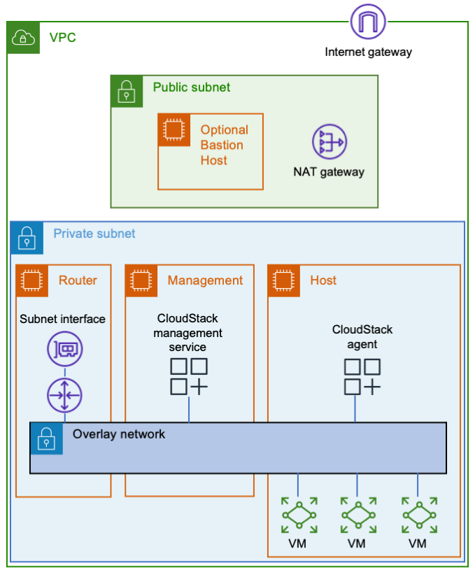
Let’s start with three Amazon EC2 instances. One will be a router between the overlay network and your Amazon VPC, the second one will be your CloudStack management server, and the third one will be your VM host. You’ll also need a way to connect to your instances, such as a bastion host or a VPN endpoint.
The router won’t need much computing power, but it will need enough network bandwidth to meet your needs. If you put Amazon EFS in the same subnet as your instances, then they’ll communicate with it directly, thereby reducing the load on the router. Decide how much network throughput you want, and then pick a suitable Nitro instance type.
After creating the router instance, configure AWS to use it as a router. Stop source/destination checking in the instance’s network settings. Then update the applicable AWS route tables to use the router as the target for the overlay network. The router’s security group needs to allow ingress to the CloudStack UI (TCP port 8080) and any services you plan to offer from VMs.
For the management server, you’ll want a Nitro instance type. It’s going to use more CPU than your router, so plan accordingly.
In addition to being a Nitro type, the host instance must also be a metal type. Metal instances have hardware virtualization support, which is needed by KVM. If you have a new AWS account with a low on-demand vCPU limit, then consider starting with an m5zn.metal, which has 48 vCPUs. Otherwise, I suggest going directly to a c5.metal because it provides 96 vCPUs for a similar price. There are bigger types available depending on your compute needs, budget, and vCPU limit. If your account’s on-demand vCPU limit is too low, then you can file a support ticket to have it raised.
Networking
All of the instances should be on a dedicated subnet. Sharing the subnet with other instances can cause communication issues. For an example, refer to the following figure. The subnet has an instance named TroubleMaker that’s not on the overlay network. If TroubleMaker sends a request to the management instance’s overlay network address, then here’s what happens:
The request goes through the AWS subnet to the router.
The router forwards the request via the overlay network.
The CloudStack management instance has a connection to the same AWS subnet that TroubleMaker is on. Therefore, it responds directly instead of using the router. This isn’t the return path that AWS is expecting, so the response is dropped.
If you move TroubleMaker to a different subnet, then the requests and responses will all go through the router. That will fix the communication issues.
The instances in the overlay network will use special interfaces that serve as VXLAN tunnel endpoints (VTEPs). The VTEPs must know how to contact each other via the underlay network. You could manually give each instance a list of all of the other instances, but that’s a maintenance nightmare. It’s better to let the VTEPs discover each other, which they can do using multicast. You can add multicast support using AWS Transit Gateway.
Here are the steps to make VXLAN multicasts work:
Enable multicast support when you create the transit gateway.
Attach the transit gateway to your subnet.
Create a transit gateway multicast domain with IGMPv2 support enabled.
Associate the multicast domain with your subnet.
Configure the eth0 interface on each instance to use IGMPv2. The following sample code shows how to do this.
Make sure that your instance security groups allow ingress for IGMP queries (protocol 2 traffic from 0.0.0.0/32) and VXLAN traffic (UDP port 4789 from the other instances).
CloudStack VMs must connect to the same bridge as the VXLAN interface. As mentioned in the previous post, CloudStack cares about names. I recommend giving the interface a name starting with “eth”. Moreover, this naming convention tells CloudStack which bridge to use, thereby avoiding the need for a dummy interface like the one in the simple setup.
The following snippet shows how I configured the networking in CentOS 7. You must provide values for these variables:
$overlay_host_ip_address, $overlay_netmask, and $overlay_gateway_ip: Use values for the overlay network that you’re creating.
$multicast_address: The multicast address that you want VXLAN to use. Pick something in the multicast range that won’t conflict with anything else. I recommend choosing from the IPv4 local scope (239.255.0.0/16).
$interface_name: The name of the interface VXLAN should use to communicate with the physical network. This is typically eth0.
A couple of the steps are different for the router instance than for the other instances. Pay attention to the comments!
yum install -y bridge-utils net-tools

# IMPORTANT: Omit the GATEWAY setting on the router instance!
cat << EOF > /etc/sysconfig/network-scripts/ifcfg-cloudbr0
DEVICE=cloudbr0
TYPE=Bridge
ONBOOT=yes
BOOTPROTO=none
IPV6INIT=no
IPV6_AUTOCONF=no
DELAY=5
STP=no
USERCTL=no
NM_CONTROLLED=no
IPADDR=$overlay_host_ip_address
NETMASK=$overlay_netmask
DNS1=$dns_address
GATEWAY=$overlay_gateway_ip
EOF

cat << EOF > /sbin/ifup-local
#!/bin/bash
# Set up VXLAN once cloudbr0 is available.
if [[ \$1 == "cloudbr0" ]]
then
    ip link add ethvxlan0 type vxlan id 100 dstport 4789 group "$multicast_address" dev "$interface_name"
    brctl addif cloudbr0 ethvxlan0
    ip link set up dev ethvxlan0
fi
EOF

chmod +x /sbin/ifup-local

# Transit Gateway requires IGMP version 2
echo "net.ipv4.conf.$interface_name.force_igmp_version=2" >> /etc/sysctl.conf
sysctl -p

# Enable IPv4 forwarding
# IMPORTANT: Only do this on the router instance!
echo 'net.ipv4.ip_forward=1' >> /etc/sysctl.conf
sysctl -p

# Restart the network service to make the changes take effect.
systemctl restart network
Storage
Let’s look at storage. Create an Amazon RDS database using the MySQL 8.0 engine, and set a master password for CloudStack’s database setup tool to use. Refer to the CloudStack documentation to find the MySQL settings that you’ll need. You can put the settings in an RDS parameter group. In case you’re wondering why I’m not using Amazon Aurora, it’s because CloudStack needs the MyISAM storage engine, which isn’t available in Aurora.
I recommend Amazon EFS for file storage. For efficiency, create a mount target in the subnet with your EC2 instances. That will enable them to communicate directly with the mount target, thereby bypassing the overlay network and router. Note that the system VMs will use Amazon EFS via the router.
If you want, you can consolidate your CloudStack file systems. Just create a single file system with directories for each zone and type of storage. For example, I use directories named /zone1/primary, /zone1/secondary, /zone2/primary, etc. You should also consider enabling provisioned throughput on the file system, or you may run out of bursting credits after booting a few VMs.
One consequence of the file system’s scalability is that the amount of free space (8 exabytes) will cause an integer overflow in CloudStack! To avoid this problem, reduce storage.overprovisioning.factor in CloudStack’s global settings from 2 to 1.
When your environment is ready, install CloudStack. When it asks for a default gateway, remember to use the router’s overlay network address. When you add a host, make sure that you use the host’s overlay network IP address.
The security groups that you created for the instances, database, and file system
Conclusion
The approach I shared has many steps, but they’re not bad when you have a plan. Whether you need a simple setup for experiments, or you need a scalable environment for a data center migration, you now have a path forward. Give it a try, and comment here about the things you learned. I hope you find it useful and fun!
“Apache”, “Apache CloudStack”, and “CloudStack” are trademarks of the Apache Software Foundation.
This blog is written by Mark Rogers, SDE II – Customer Engineering AWS.
How do you put a cloud inside another cloud? Some features that make Amazon Elastic Compute Cloud (Amazon EC2) secure and wonderful also make running CloudStack difficult. The biggest obstacle is that AWS and CloudStack both want to manage network resources. Therefore, we must keep them out of each other’s way. This requires some steps that aren’t obvious, and it took a long time to figure out. I’m going to share what I learned, so that you can navigate the process more easily.
Apache CloudStack is an open-source platform for deploying and managing virtual machines (VMs) and the associated network and storage infrastructure. You would normally run it on your own hardware to create your own cloud. But there can be advantages to running it inside of an Amazon Virtual Private Cloud (Amazon VPC), including how it could help you migrate out of a data center. It’s a great way to create disposable environments for experiments or training. Furthermore, it’s a convenient way to test-drive the new CloudStack support in Amazon Elastic Kubernetes Service (Amazon EKS) Anywhere. In my case, I needed to create development and test environments for a project that uses the CloudStack API. The environments needed to be shared and scalable. Our build pipelines were already in AWS, so it made sense to put the new environments there, too.
CloudStack can work with a number of hypervisors. The instructions in this article will use Kernel-based Virtual Machine (KVM) on Linux. KVM will manage the VMs at a low level, and CloudStack will manage KVM.
Prerequisites
Most of the information in this article should be applicable to a range of CloudStack versions. I targeted CloudStack 4.14 on CentOS 7. I also tested CloudStack versions 4.16 and 4.17, and I recommend them.
The official CentOS 7 x86_64 HVM image works well. If you use a different Linux flavor or version, then you might have to modify some of the implementation details.
You’ll need to know the basics of CloudStack. The scope of this article is making CloudStack and AWS coexist peacefully. Once CloudStack is running, I’m assuming that you’ll handle things from there. Refer to the AWS documentation and CloudStack documentation for information on security and other best practices.
Making things easier
I wrote some scripts to automate the installation. You can run them on EC2 instances with CentOS 7, and they’ll do all the installation and OS configuration for you. You can use them as they are, or customize them to meet your needs. I also wrote some AWS CloudFormation templates you can copy in order to create a demo environment. The README file has more details.
I like c5.metal because it’s one of the least expensive metal types, and has a low cost per vCPU. It has 96 vCPUs and 192 GiB of memory. If you run 20 VMs on it, with 4 CPU cores and 8 GiB of memory each, then you’d still have 16 vCPUs and 32 GiB to share between the operating system, CloudStack, and MySQL. Using CloudStack’s overprovisioning feature, you could fit even more VMs if they’re running light loads.
Networking
The biggest challenge is the network. AWS knows which IP and MAC addresses should exist, and it knows the machines to which they should belong. It blocks any traffic that doesn’t fit its idea of how the network should behave. Simultaneously, CloudStack assumes that any IP or MAC address it invents should work just fine. When CloudStack assigns addresses to VMs on an AWS subnet, their network traffic gets blocked.
You could get around this by enabling network address translation (NAT) on the instance running CloudStack. That’s a great solution if it fits your needs, but it makes it hard for other machines in your Amazon VPC to contact your VMs. I recommend a different approach.
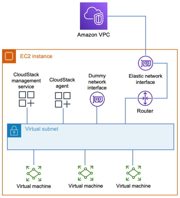
Although AWS restricts what you can do with its layer 2 network, it’s perfectly happy to let you run your own layer 3 router. Your EC2 instance can act as a router to a new virtual subnet that’s outside of the jurisdiction of AWS. The instance integrates with AWS just like a VPN appliance, routing traffic to wherever it needs to go. CloudStack can do whatever it wants in the virtual subnet, and everybody’s happy.
What do I mean by a virtual subnet? This is a subnet that exists only inside the EC2 instance. It consists of logical network interfaces attached to a Linux bridge. The entire subnet exists inside a single EC2 instance. It doesn’t scale well, but it’s simple. In my next post, I’ll cover a more complicated setup with an overlay network that spans multiple instances to allow horizontal scaling.
The simple way
The simple way is to put everything in one EC2 instance, including the database, file storage, and a virtual subnet. Because everything’s stored locally, allocate enough disk space for your needs. 500 GB will be enough to support a few basic VMs. Create or select a security group for your instance that gives users access to the CloudStack UI (TCP port 8080). The security group should also allow access to any services that you’ll offer from your VMs.
When you have your instance, configure AWS to treat it as a router.
a. Go to the VPC settings, and select Route Tables.
b. Identify the tables for subnets that need CloudStack access.
c. In each of these tables, add a route to the new virtual subnet. The route target should be your EC2 instance.
4. Depending on your network needs, you may also need to add routes to transit gateways, VPN endpoints, etc.
Because everything will be on one server, creating a virtual subnet is simply a matter of creating a Linux bridge. CloudStack must find a network adapter attached to the bridge. Therefore, add a dummy interface with a name that CloudStack will recognize.
The following snippet shows how I configure networking in CentOS 7. You must provide values for the variables $virutal_host_ip_address and $virtual_netmask to reflect the virtual subnet that you want to create. For $dns_address, I recommend the base of the VPC IPv4 network range, plus two. You shouldn’t use 169.654.169.253 because CloudStack reserves link-local addresses for its own use.
yum install -y bridge-utils net-tools

# The bridge must be named cloudbr0.

cat << EOF > /etc/sysconfig/network-scripts/ifcfg-cloudbr0
DEVICE=cloudbr0
TYPE=Bridge
ONBOOT=yes
BOOTPROTO=none
IPV6INIT=no
IPV6_AUTOCONF=no
DELAY=5
STP=yes
USERCTL=no
NM_CONTROLLED=no
IPADDR=$virtual_host_ip_address
NETMASK=$virtual_netmask
DNS1=$dns_address
EOF

# Create a dummy network interface.
cat << EOF > /etc/sysconfig/modules/dummy.modules
#!/bin/sh
/sbin/modprobe dummy numdummies=1
/sbin/ip link set name ethdummy0 dev dummy0
EOF

chmod +x /etc/sysconfig/modules/dummy.modules
/etc/sysconfig/modules/dummy.modules

cat << EOF > /etc/sysconfig/network-scripts/ifcfg-ethdummy0
TYPE=Ethernet
BOOTPROTO=none
NAME=ethdummy0
DEVICE=ethdummy0
ONBOOT=yes
BRIDGE=cloudbr0
NM_CONTROLLED=no
EOF

# Turn the instance into a router

echo 'net.ipv4.ip_forward=1' >> /etc/sysctl.conf
sysctl -p

# Must kill dhclient or the network service won't restart properly.
# A reboot would also work, if you’d rather do that.

pkill dhclient
systemctl restart network
CloudStack must know which IP addresses to use for inter-service communication. It will select by resolving the machine’s fully qualified domain name (FQDN) to an address. The following commands will make it to choose the right one. You must provide a value for $virtual_host_ip_address.
Remember that CloudStack is only directly connected to your virtual network. The EC2 instance is the router that connects the virtual subnet to the Amazon VPC. When you’re configuring CloudStack, use your instance’s virtual subnet address as the default gateway.
To access CloudStack from your workstation, you’ll need a connection to your VPC. This can be through a client VPN or a bastion host. If you use a bastion, its subnet needs a route to your virtual subnet, and you’ll need an SSH tunnel for your browser to access the CloudStack UI. The UI is at http://x.x.x.x:8080/client/, where x.x.x.x is your CloudStack instance’s virtual subnet address. Note that CloudStack’s console viewer won’t work if you’re using an SSH tunnel.
If you’re just experimenting with CloudStack, then I suggest saving money by stopping your instance when it isn’t needed. The safe way to do that is:
Disable your zone in the CloudStack UI.
Put the primary storage into maintenance mode.
Wait for the switch to maintenance mode to be complete.
Stop the EC2 instance.
When you’re ready to turn everything back on, simply reverse those steps. If you have any virtual routers in CloudStack, then you may need to start those, too.
Getting CloudStack to run on AWS isn’t so bad. The hardest part is simply knowing how. The setup explained here is great for small installations, but it can only scale vertically. In my next post, I’ll show you how to create an installation that scales horizontally. Instead of using a virtual subnet that exists in a single EC2 instance, we’ll build an overlay network that spans multiple instances. It will use more components and features, including some that might be new to you. I hope you find it interesting!
Now that you can create a simple setup, give it a try! I hope you have fun and learn something new along the way. Comment with the results of your experiments.
“Apache”, “Apache CloudStack”, and “CloudStack” are trademarks of the Apache Software Foundation.
Amazon Macie is a fully managed data security service that uses machine learning and pattern matching to help you discover and protect sensitive data in Amazon Simple Storage Service (Amazon S3). With Macie, you can analyze objects in your S3 buckets to detect occurrences of sensitive data, such as personally identifiable information (PII), financial information, personal health information, and access credentials.
In this post, we walk you through a solution to gain comprehensive and organization-wide visibility into which types of sensitive data are present in your S3 storage, where the data is located, and how much is present. Once enabled, Macie automatically starts discovering sensitive data in your S3 storage and builds a sensitive data profile for each bucket. The profiles are organized in a visual, interactive data map, and you can use the data map to run targeted sensitive data discovery jobs. Both automated data discovery and targeted jobs produce rich, detailed sensitive data discovery results. This solution uses Amazon Athena and Amazon QuickSight to deep-dive on the Macie results, and to help you analyze, visualize, and report on sensitive data discovered by Macie, even when the data is distributed across millions of objects, thousands of S3 buckets, and thousands of AWS accounts. Athena is an interactive query service that makes it simpler to analyze data directly in Amazon S3 using standard SQL. QuickSight is a cloud-scale business intelligence tool that connects to multiple data sources, including Athena databases and tables.
This solution is relevant to data security, data governance, and security operations engineering teams.
The challenge: how to summarize sensitive data discovered in your growing S3 storage
Macie issues findings when an object is found to contain sensitive data. In addition to findings, Macie keeps a record of each S3 object analyzed in a bucket of your choice for long-term storage. These records are known as sensitive data discovery results, and they include additional context about your data in Amazon S3. Due to the large size of the results file, Macie exports the sensitive data discovery results to an S3 bucket, so you need to take additional steps to query and visualize the results. We discuss the differences between findings and results in more detail later in this post.
With the increasing number of data privacy guidelines and compliance mandates, customers need to scale their monitoring to encompass thousands of S3 buckets across their organization. The growing volume of data to assess, and the growing list of findings from discovery jobs, can make it difficult to review and remediate issues in a timely manner. In addition to viewing individual findings for specific objects, customers need a way to comprehensively view, summarize, and monitor sensitive data discovered across their S3 buckets.
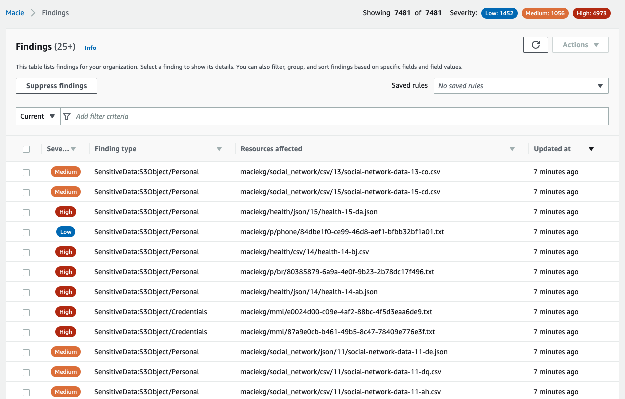
To illustrate this point, we ran a Macie sensitive data discovery job on a dataset created by AWS. The dataset contains about 7,500 files that have sensitive information, and Macie generated a finding for each sensitive file analyzed, as shown in Figure 1.
Figure 1: Macie findings from the dataset
Your security team could spend days, if not months, analyzing these individual findings manually. Instead, we outline how you can use Athena and QuickSight to query and visualize the Macie sensitive data discovery results to understand your data security posture.
The additional information in the sensitive data discovery results will help you gain comprehensive visibility into your data security posture. With this visibility, you can answer questions such as the following:
What are the top 5 most commonly occurring sensitive data types?
Which AWS accounts have the most findings?
How many S3 buckets are affected by each of the sensitive data types?
Your security team can write their own customized queries to answer questions such as the following:
Is there sensitive data in AWS accounts that are used for development purposes?
Is sensitive data present in S3 buckets that previously did not contain sensitive information?
Was there a change in configuration for S3 buckets containing the greatest amount of sensitive data?
Findings provide a report of potential policy violations with an S3 bucket, or the presence of sensitive data in a specific S3 object. Each finding provides a severity rating, information about the affected resource, and additional details, such as when Macie found the issue. Findings are published to the Macie console, AWS Security Hub, and Amazon EventBridge.
In contrast, results are a collection of records for each S3 object that a Macie job analyzed. These records contain information about objects that do and do not contain sensitive data, including up to 1,000 occurrences of each sensitive data type that Macie found in a given object, and whether Macie was unable to analyze an object because of issues such as permissions settings or use of an unsupported format. If an object contains sensitive data, the results record includes detailed information that isn’t available in the finding for the object.
One of the key benefits of querying results is to uncover gaps in your data protection initiatives—these gaps can occur when data in certain buckets can’t be analyzed because Macie was denied access to those buckets, or was unable to decrypt specific objects. The following table maps some of the key differences between findings and results.
Findings
Results
Enabled by default
Yes
No
Location of published results
Macie console, Security Hub, and EventBridge
S3 bucket
Details of S3 objects that couldn’t be scanned
No
Yes
Details of S3 objects in which no sensitive data was found
No
Yes
Identification of files inside compressed archives that contain sensitive data
No
Yes
Number of occurrences reported per object
Up to 15
Up to 1,000
Retention period
90 days in Macie console
Defined by customer
Architecture
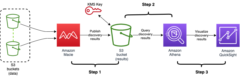
As shown in Figure 2, you can build out the solution in three steps:
Enable the results and publish them to an S3 bucket
Build out the Athena table to query the results by using SQL
Visualize the results with QuickSight
Figure 2: Architecture diagram showing the flow of the solution
Prerequisites
To implement the solution in this blog post, you must first complete the following prerequisites:
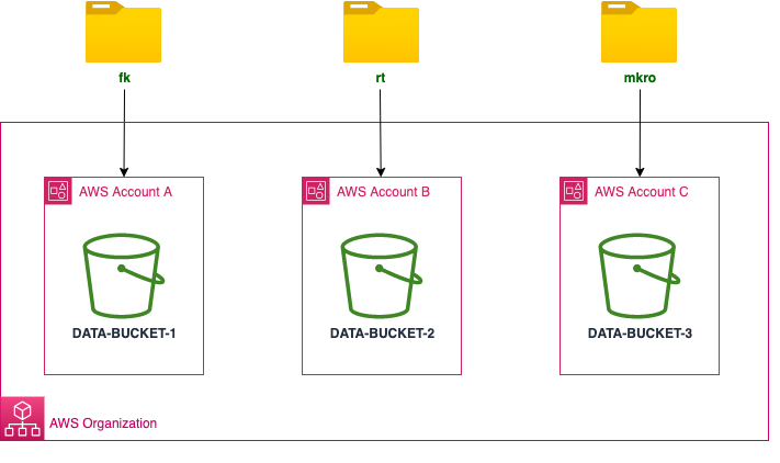
To follow along with the examples in this post, download the sample dataset. The dataset is a single .ZIP file that contains three directories (fk, rt, and mkro). For this post, we used three accounts in our organization, created an S3 bucket in each of them, and then copied each directory to an individual bucket, as shown in Figure 3.
Figure 3: Sample data loaded into three different AWS accounts
Note: All data in this blog post has been artificially created by AWS for demonstration purposes and has not been collected from any individual person. Similarly, such data does not, nor is it intended, to relate back to any individual person.
Step 1: Enable the results and publish them to an S3 bucket
Publication of the discovery results to Amazon S3 is not enabled by default. The setup requires that you specify an S3 bucket to store the results (we also refer to this as the discovery results bucket), and use an AWS Key Management Service (AWS KMS) key to encrypt the bucket.
If you are analyzing data across multiple accounts in your organization, then you need to enable the results in your delegated Macie administrator account. You do not need to enable results in individual member accounts. However, if you’re running Macie jobs in a standalone account, then you should enable the Macie results directly in that account.
Select the AWS Region from the upper right of the page.
From the left navigation pane, select Discovery results.
Select Configure now.
Select Create Bucket, and enter a unique bucket name. This will be the discovery results bucket name. Make note of this name because you will use it when you configure the Athena tables later in this post.
Under Encryption settings, select Create new key. This takes you to the AWS KMS console in a new browser tab.
In the AWS KMS console, do the following:
For Key type, choose symmetric, and for Key usage, choose Encrypt and Decrypt.
Enter a meaningful key alias (for example, macie-results-key) and description.
(Optional) For simplicity, set your current user or role as the Key Administrator.
Set your current user/role as a user of this key in the key usage permissions step. This will give you the right permissions to run the Athena queries later.
From the AWS KMS Key dropdown, select the new key.
To view KMS key policy statements that were automatically generated for your specific key, account, and Region, select View Policy. Copy these statements in their entirety to your clipboard.
Navigate back to the browser tab with the AWS KMS console and then do the following:
Select Customer managed keys.
Choose the KMS key that you created, choose Switch to policy view, and under Key policy, select Edit.
In the key policy, paste the statements that you copied. When you add the statements, do not delete any existing statements and make sure that the syntax is valid. Policies are in JSON format.
Review the inputs in the Settings page for Discovery results and then choose Save. Macie will perform a check to make sure that it has the right access to the KMS key, and then it will create a new S3 bucket with the required permissions.
If you haven’t run a Macie discovery job in the last 90 days, you will need to run a new discovery job to publish the results to the bucket.
In this step, you created a new S3 bucket and KMS key that you are using only for Macie. For instructions on how to enable and configure the results using existing resources, see Storing and retaining sensitive data discovery results with Amazon Macie. Make sure to review Macie pricing details before creating and running a sensitive data discovery job.
Step 2: Build out the Athena table to query the results using SQL
Now that you have enabled the discovery results, Macie will begin publishing them into your discovery results bucket in the form of jsonl.gz files. Depending on the amount of data, there could be thousands of individual files, with each file containing multiple records. To identify the top five most commonly occurring sensitive data types in your organization, you would need to query all of these files together.
In this step, you will configure Athena so that it can query the results using SQL syntax. Before you can run an Athena query, you must specify a query result bucket location in Amazon S3. This is different from the Macie discovery results bucket that you created in the previous step.
If you haven’t set up Athena previously, we recommend that you create a separate S3 bucket, and specify a query result location using the Athena console. After you’ve set up the query result location, you can configure Athena.
To create a new Athena database and table for the Macie results
Open the Athena console, and in the query editor, enter the following data definition language (DDL) statement. In the context of SQL, a DDL statement is a syntax for creating and modifying database objects, such as tables. For this example, we named our database macie_results.
CREATE DATABASE macie_results;
After running this step, you’ll see a new database in the Database dropdown. Make sure that the new macie_results database is selected for the next queries.
Figure 4: Create database in the Athena console
Create a table in the database by using the following DDL statement. Make sure to replace <RESULTS-BUCKET-NAME> with the name of the discovery results bucket that you created previously.
CREATE EXTERNAL TABLE maciedetail_all_jobs(
	accountid string,
	category string,
	classificationdetails struct<jobArn:string,result:struct<status:struct<code:string,reason:string>,sizeClassified:string,mimeType:string,sensitiveData:array<struct<category:string,totalCount:string,detections:array<struct<type:string,count:string,occurrences:struct<lineRanges:array<struct<start:string,`end`:string,`startColumn`:string>>,pages:array<struct<pageNumber:string>>,records:array<struct<recordIndex:string,jsonPath:string>>,cells:array<struct<row:string,`column`:string,`columnName`:string,cellReference:string>>>>>>>,customDataIdentifiers:struct<totalCount:string,detections:array<struct<arn:string,name:string,count:string,occurrences:struct<lineRanges:array<struct<start:string,`end`:string,`startColumn`:string>>,pages:array<string>,records:array<string>,cells:array<string>>>>>>,detailedResultsLocation:string,jobId:string>,
	createdat string,
	description string,
	id string,
	partition string,
	region string,
	resourcesaffected struct<s3Bucket:struct<arn:string,name:string,createdAt:string,owner:struct<displayName:string,id:string>,tags:array<string>,defaultServerSideEncryption:struct<encryptionType:string,kmsMasterKeyId:string>,publicAccess:struct<permissionConfiguration:struct<bucketLevelPermissions:struct<accessControlList:struct<allowsPublicReadAccess:boolean,allowsPublicWriteAccess:boolean>,bucketPolicy:struct<allowsPublicReadAccess:boolean,allowsPublicWriteAccess:boolean>,blockPublicAccess:struct<ignorePublicAcls:boolean,restrictPublicBuckets:boolean,blockPublicAcls:boolean,blockPublicPolicy:boolean>>,accountLevelPermissions:struct<blockPublicAccess:struct<ignorePublicAcls:boolean,restrictPublicBuckets:boolean,blockPublicAcls:boolean,blockPublicPolicy:boolean>>>,effectivePermission:string>>,s3Object:struct<bucketArn:string,key:string,path:string,extension:string,lastModified:string,eTag:string,serverSideEncryption:struct<encryptionType:string,kmsMasterKeyId:string>,size:string,storageClass:string,tags:array<string>,embeddedFileDetails:struct<filePath:string,fileExtension:string,fileSize:string,fileLastModified:string>,publicAccess:boolean>>,
	schemaversion string,
	severity struct<description:string,score:int>,
	title string,
	type string,
	updatedat string)
ROW FORMAT SERDE
	'org.openx.data.jsonserde.JsonSerDe'
WITH SERDEPROPERTIES (
	'paths'='accountId,category,classificationDetails,createdAt,description,id,partition,region,resourcesAffected,schemaVersion,severity,title,type,updatedAt')
STORED AS INPUTFORMAT
	'org.apache.hadoop.mapred.TextInputFormat'
OUTPUTFORMAT
	'org.apache.hadoop.hive.ql.io.HiveIgnoreKeyTextOutputFormat'
LOCATION
	's3://<RESULTS-BUCKET-NAME>/AWSLogs/'
After you complete this step, you will see a new table named maciedetail_all_jobs in the Tables section of the query editor.
Query the results to start gaining insights. For example, to identify the top five most common sensitive data types, run the following query:
select sensitive_data.category,
	detections_data.type,
	sum(cast(detections_data.count as INT)) total_detections
from maciedetail_all_jobs,
	unnest(classificationdetails.result.sensitiveData) as t(sensitive_data),
	unnest(sensitive_data.detections) as t(detections_data)
where classificationdetails.result.sensitiveData is not null
and resourcesaffected.s3object.embeddedfiledetails is null
group by sensitive_data.category, detections_data.type
order by total_detections desc
LIMIT 5
Running this query on the sample dataset gives the following output.
Figure 5: Results of a query showing the five most common sensitive data types in the dataset
(Optional) The previous query ran on all of the results available for Macie. You can further query which accounts have the greatest amount of sensitive data detected.
select accountid,
	sum(cast(detections_data.count as INT)) total_detections
from maciedetail_all_jobs,
	unnest(classificationdetails.result.sensitiveData) as t(sensitive_data),
	unnest(sensitive_data.detections) as t(detections_data)
where classificationdetails.result.sensitiveData is not null
and resourcesaffected.s3object.embeddedfiledetails is null
group by accountid
order by total_detections desc
To test this query, we distributed the synthetic dataset across three member accounts in our organization, ran the query, and received the following output. If you enable Macie in just a single account, then you will only receive results for that one account.
Figure 6: Query results for total number of sensitive data detections across all accounts in an organization
In the previous step, you used Athena to query your Macie discovery results. Although the queries were powerful, they only produced tabular data as their output. In this step, you will use QuickSight to visualize the results of your Macie jobs.
Before creating the visualizations, you first need to grant QuickSight the right permissions to access Athena, the results bucket, and the KMS key that you used to encrypt the results.
Paste the following statement in the key policy. When you add the statement, do not delete any existing statements, and make sure that the syntax is valid. Replace <QUICKSIGHT_SERVICE_ROLE_ARN> and <KMS_KEY_ARN> with your own information. Policies are in JSON format.
	{ "Sid": "Allow Quicksight Service Role to use the key",
		"Effect": "Allow",
		"Principal": {
			"AWS": <QUICKSIGHT_SERVICE_ROLE_ARN>
		},
		"Action": "kms:Decrypt",
		"Resource": <KMS_KEY_ARN>
	}
To allow QuickSight access to Athena and the discovery results S3 bucket
In QuickSight, in the upper right, choose your user icon to open the profile menu, and choose US East (N.Virginia). You can only modify permissions in this Region.
In the upper right, open the profile menu again, and select Manage QuickSight.
Select Security & permissions.
Under QuickSight access to AWS services, choose Manage.
Make sure that the S3 checkbox is selected, click on Select S3 buckets, and then do the following:
Choose the discovery results bucket.
You do not need to check the box under Write permissions for Athena workgroup. The write permissions are not required for this post.
Select Finish.
Make sure that the Amazon Athena checkbox is selected.
Review the selections and be careful that you don’t inadvertently disable AWS services and resources that other users might be using.
Select Save.
In QuickSight, in the upper right, open the profile menu, and choose the Region where your results bucket is located.
Now that you’ve granted QuickSight the right permissions, you can begin creating visualizations.
To create a new dataset referencing the Athena table
On the QuickSight start page, choose Datasets.
On the Datasets page, choose New dataset.
From the list of data sources, select Athena.
Enter a meaningful name for the data source (for example, macie_datasource) and choose Create data source.
Select the database that you created in Athena (for example, macie_results).
Select the table that you created in Athena (for example, maciedetail_all_jobs), and choose Select.
You can either import the data into SPICE or query the data directly. We recommend that you use SPICE for improved performance, but the visualizations will still work if you query the data directly.
To create an analysis using the data as-is, choose Visualize.
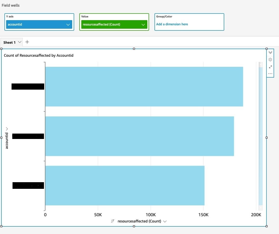
You can then visualize the Macie results in the QuickSight console. The following example shows a delegated Macie administrator account that is running a visualization, with account IDs on the y axis and the count of affected resources on the x axis.
Figure 7: Visualize query results to identify total number of sensitive data detections across accounts in an organization
You can also visualize the aggregated data in QuickSight. For example, you can view the number of findings for each sensitive data category in each S3 bucket. The Athena table doesn’t provide aggregated data necessary for visualization. Instead, you need to query the table and then visualize the output of the query.
To query the table and visualize the output in QuickSight
On the Amazon QuickSight start page, choose Datasets.
On the Datasets page, choose New dataset.
Select the data source that you created in Athena (for example, macie_datasource) and then choose Create Dataset.
Select the database that you created in Athena (for example, macie_results).
Choose Use Custom SQL, enter the following query below, and choose Confirm Query.
	select resourcesaffected.s3bucket.name as bucket_name,
		sensitive_data.category,
		detections_data.type,
		sum(cast(detections_data.count as INT)) total_detections
	from macie_results.maciedetail_all_jobs,
		unnest(classificationdetails.result.sensitiveData) as t(sensitive_data),unnest(sensitive_data.detections) as t(detections_data)
where classificationdetails.result.sensitiveData is not null
and resourcesaffected.s3object.embeddedfiledetails is null
group by resourcesaffected.s3bucket.name, sensitive_data.category, detections_data.type
order by total_detections desc
You can either import the data into SPICE or query the data directly.
To create an analysis using the data as-is, choose Visualize.
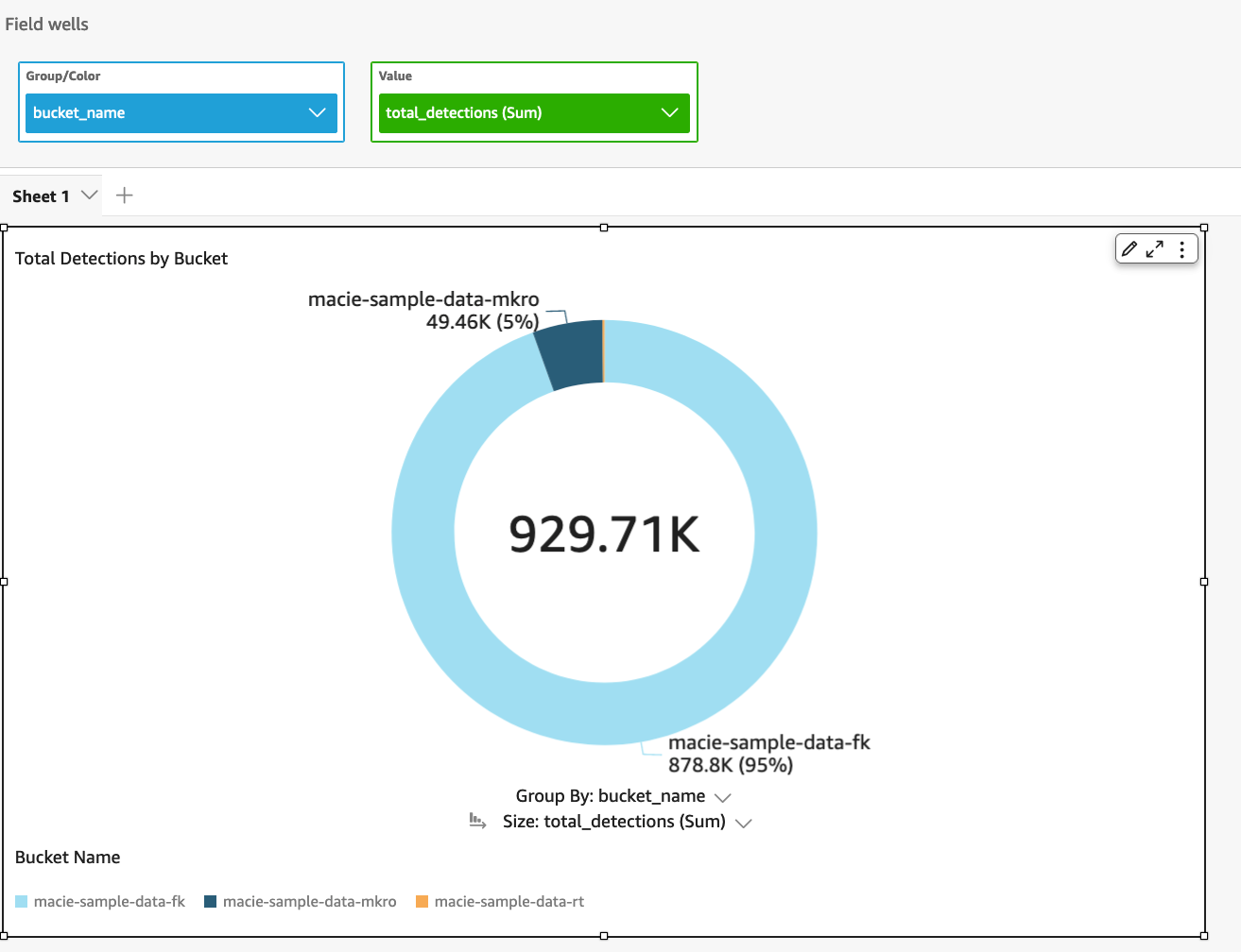
Now you can visualize the output of the query that aggregates data across your S3 buckets. For example, we used the name of the S3 bucket to group the results, and then we created a donut chart of the output, as shown in Figure 6.
Figure 8: Visualize query results for total number of sensitive data detections across each S3 bucket in an organization
From the visualizations, we can identify which buckets or accounts in our organizations contain the most sensitive data, for further action. Visualizations can also act as a dashboard to track remediation.
You can replicate the preceding steps by using the sample queries from the amazon-macie-results-analytics GitHub repo to view data that is aggregated across S3 buckets, AWS accounts, or individual Macie jobs. Using these queries with the results of your Macie results will help you get started with tracking the security posture of your data in Amazon S3.
Conclusion
In this post, you learned how to enable sensitive data discovery results for Macie, query those results with Athena, and visualize the results in QuickSight.
Because Macie sensitive data discovery results provide more granular data than the findings, you can pursue a more comprehensive incident response when sensitive data is discovered. The sample queries in this post provide answers to some generic questions that you might have. After you become familiar with the structure, you can run other interesting queries on the data.
We hope that you can use this solution to write your own queries to gain further insights into sensitive data discovered in S3 buckets, according to the business needs and regulatory requirements of your organization. You can consider using this solution to better understand and identify data security risks that need immediate attention. For example, you can use this solution to answer questions such as the following:
Is financial information present in an AWS account where it shouldn’t be?
Are S3 buckets that contain PII properly hardened with access controls and encryption?
You can also use this solution to understand gaps in your data security initiatives by tracking files that Macie couldn’t analyze due to encryption or permission issues. To further expand your knowledge of Macie capabilities and features, see the following resources:
If you have feedback about this post, submit comments in the Comments section below. If you have questions about this post, start a new thread on Amazon Macie re:Post.
Want more AWS Security news? Follow us on Twitter.
Most developers probably do not see the generation of random numbers as
being a performance bottleneck for their programs, but there are seemingly
exceptions. Over the last few years, Jason Donenfeld has brought a new
level of energy to the development of the kernel’s random-number generator;
he is now directing his efforts toward improving performance for user space
with this patch
series that provides an implementation of the getrandom()
system call in the kernel’s “virtual dynamic
shared object” (vDSO) area. The result is, indeed, better performance,
but not all developers see this benefit as being worth the additional
complexity required to achieve it.
Amazon CodeCatalyst is a modern software development service that empowers teams to deliver software on AWS easily and quickly. CodeCatalyst provides one place where you can plan, code, and build, test, and deploy applications with continuous integration/continuous delivery (CI/CD) tools. It also helps streamlined team collaboration. Developers on modern software teams are usually distributed, work independently, and use disparate tools. Often, ad hoc collaboration is necessary to resolve problems. Today, developers are forced to do this across many tools, which distract developers from their primary task—adding business critical features and enhancing their quality and completeness.
In this post, we explain how Contino uses CodeCatalyst to on-board their engineering team onto new projects, eliminates the overhead of managing disparate tools, and streamlines collaboration among different stakeholders.
The Problem
Contino helps customers migrate their applications to the cloud, and then improves their architecture by taking full advantage of cloud-native features to improve agility, performance, and scalability. This usually involves the build out of a central landing zone platform. A landing zone is a set of standard building blocks that allows customers to automatically create accounts, infrastructure and environments that are pre-configured in line with security policies, compliance guidelines and cloud native best practices. Some features are common to most landing zones, for example creating secure container images, AMIs, and environment setup boilerplate. In order to provide maximum value to the customers, Contino develops in-house versions of such features, incorporating AWS best practices, and later rolls out to the customer’s environment with some customization. Contino’s technical consultants, who are not currently assigned to customer work, collectively known as ‘Squad 0’ work on these features. Squad 0 builds the foundation for the work that will be re-used by other squads that work directly with Contino’s customers. As the technical consultants are typically on Squad 0 for a short period, it is critical that they can be productive in this short time, without spending too much time getting set up.
To build these foundational services, Contino was looking for something more integrated that would allow them to quickly setup development environments, enable collaboration between Squad 0 members, invite other squads to validate foundations services usage for their respective customers, and provide access to different AWS accounts and git repos centrally from one place. Historically, Contino has used disparate tools to achieve this, which meant having to grant/revoke access to the various AWS accounts individually on a continual basis. With these disparate tools, granting access to the tools needed for squads to be productive was non-trivial.
The Solution
It was at this point Contino participated in the private beta for CodeCatalyst prior to the public preview. CodeCatalyst has allowed Contino to move to a structure, as shown in Figure 1 below. A Project Manager at Contino creates a different project for each foundational service and invites Squad 0 members to join the relevant project. With CodeCatalyst, Squad 0 technical consultants use features like CI/CD, source repositories, and issue trackers to build foundational services. This helps eliminate the overhead of managing and integrating developer tools and provides more time to focus on developing code. Once Squad 0 is ready with the foundational services, they invite customer squads using their email address to validate the readiness of the project for use with their customers. Finally, members of Squad 0 use Cloud 9 Dev Environments from within CodeCatalyst to rapidly create consistent cloud development environments, without manual configuration, so they can work on new or multiple projects simultaneously, without conflict.
Figure 1: CodeCatalyst with multiple account connections
Contino uses CI/CD to conduct multi-account deployments. Contino typically does one of two types of deployments: 1. Traditional sequential application deployment that is promoted from one environment to another, for example dev -> test -> prod, and 2. Parallel deployment, for example, a security control that is required to be deployed out into multiple AWS accounts at the same time. CodeCatalyst solves this problem by making it easier to construct workflows using a workflow definition file that can deploy either sequentially or in parallel to multiple AWS accounts. Figure 2 shows parallel deployment.
Figure 2: CI/CD with CodeCatalyst
The Value
CodeCatalyst has reduced the time it takes for members of Squad 0 to complete the necessary on-boarding to work on foundational services from 1.5 days to about 1 hour. These tasks include setting up connections to source repositories, setting up development environments, configuring IAM roles and trust relationships, etc. With support for integrated tools and better collaboration, CodeCatalyst minimized overhead for ad hoc collaboration. Squad 0 could spend more time on writing code to build foundation services. This has led to tasks being completed, on average, 20% faster. This increased productivity led to increased value delivered to Contino’s customers. As Squad 0 is more productive, more foundation services are available for other squads to reuse for their respective customers. Now, Contino’s teams on the ground working directly with customers can re-use these services with some customization for the specific needs of the customer.
Conclusion
Amazon CodeCatalyst brings together everything software development teams need to plan, code, build, test, and deploy applications on AWS into a streamlined, integrated experience. With CodeCatalyst, developers can spend more time developing application features and less time setting up project tools, creating and managing CI/CD pipelines, provisioning and configuring various development environments or coordinating with team members. With CodeCatalyst, the Contino engineers can improve productivity and focus on rapidly developing application code which captures business value for their customers.
Security updates have been issued by Debian (libetpan and smarty3), SUSE (libksba, rpmlint-mini, tcl, and xrdp), and Ubuntu (curl, firefox, and linux-oem-5.14).
Peter Hutterer writes
about the disabling of support for byte-swapped clients in the X.org server
and the reasons why this was done.
These days, encountering a Big Endian host is increasingly niche,
letting it run an X client that connects to your local
little-endian X server is even more niche. I think the only
regular real-world use-case for this is running X clients on an
s390x, connecting to your local intel-ish (and thus little endian)
workstation. Not something most users do on a regular basis. So
right now, the byte-swapping code is mainly a free attack surface
that 99% of users never actually use for anything real. So… let’s
not do that?
The collective thoughts of the interwebz
Manage Consent
To provide the best experiences, we use technologies like cookies to store and/or access device information. Consenting to these technologies will allow us to process data such as browsing behavior or unique IDs on this site. Not consenting or withdrawing consent, may adversely affect certain features and functions.
Functional
Always active
The technical storage or access is strictly necessary for the legitimate purpose of enabling the use of a specific service explicitly requested by the subscriber or user, or for the sole purpose of carrying out the transmission of a communication over an electronic communications network.
Preferences
The technical storage or access is necessary for the legitimate purpose of storing preferences that are not requested by the subscriber or user.
Statistics
The technical storage or access that is used exclusively for statistical purposes.The technical storage or access that is used exclusively for anonymous statistical purposes. Without a subpoena, voluntary compliance on the part of your Internet Service Provider, or additional records from a third party, information stored or retrieved for this purpose alone cannot usually be used to identify you.
Marketing
The technical storage or access is required to create user profiles to send advertising, or to track the user on a website or across several websites for similar marketing purposes.
 comments




 Aish Gunasekar is a Specialist Solutions architect with a focus on Amazon OpenSearch Service. Her passion at AWS is to help customers design highly scalable architectures and help them in their cloud adoption journey. Outside of work, she enjoys hiking and baking.
 Pavani Baddepudi is a senior product manager working in search services at AWS. Her interests include distributed systems, networking, and security.