Security updates for Wednesday

Post Syndicated from original https://lwn.net/Articles/892047/

Security updates have been issued by Debian (condor), Red Hat (389-ds:1.4, container-tools:2.0, kernel, kernel-rt, and kpatch-patch), SUSE (chrony, containerd, expat, git, icedtea-web, jsoup, jsr-305, kernel, libeconf, shadow and util-linux, protobuf, python-libxml2-python, python3, slirp4netns, sssd, vim, and wpa_supplicant), and Ubuntu (bash).

The More You Know, The More You Know You Don’t Know (Project Zero)

Post Syndicated from original https://lwn.net/Articles/891959/

The Google Project Zero blog is carrying a
report on zero-day vulnerabilities
found to be exploited during 2021.

5 of the 7 [Android] 0-days from 2021 targeted GPU drivers. This is
actually
not that surprising when we consider the evolution of the Android
ecosystem as well as recent public security research into
Android. The Android ecosystem is quite fragmented: many different
kernel versions, different manufacturer customizations, etc. If an
attacker wants a capability against “Android devices”, they
generally need to maintain many different exploits to have a decent
percentage of the Android ecosystem covered. However, if the
attacker chooses to target the GPU kernel driver instead of another
component, they will only need to have two exploits since most
Android devices use 1 of 2 GPUs: either the Qualcomm Adreno GPU or
the ARM Mali GPU.

Amazon Redshift continues its price-performance leadership

Post Syndicated from Stefan Gromoll original https://aws.amazon.com/blogs/big-data/amazon-redshift-continues-its-price-performance-leadership/

Data is a strategic asset. Getting timely value from data requires high-performance systems that can deliver performance at scale while keeping costs low. Amazon Redshift is the most popular cloud data warehouse that is used by tens of thousands of customers to analyze exabytes of data every day. We continue to add new capabilities to improve the price-performance ratio for our customers as you bring more data to your Amazon Redshift environments.

This post goes into detail on the analytic workload trends we’re seeing from the Amazon Redshift fleet’s telemetry data, new capabilities we have launched to improve Amazon Redshift’s price-performance, and the results from the latest benchmarks derived from TPC-DS and TPC-H, which reenforce our leadership.

Data-driven performance optimization

We relentlessly focus on improving Amazon Redshift’s price-performance so that you continue to see improvements in your real-world workloads. To this end, the Amazon Redshift team takes a data-driven approach to performance optimization. Werner Vogels discussed our methodology in Amazon Redshift and the art of performance optimization in the cloud, and we have continued to focus our efforts on using performance telemetry from our large customer base to drive the Amazon Redshift performance improvements that matter most to our customers.

At this point, you might ask why does price-performance matter? One critical aspect of a data warehouse is how it scales as your data grows. Will you be paying more per TB as you add more data, or will your costs remain consistent and predictable? We work to make sure that Amazon Redshift delivers not only strong performance as your data grows, but also consistent price-performance.

Optimizing high-concurrency, low-latency workloads

One of the trends that we have observed is that customers are increasingly building analytics applications that require high concurrency of low-latency queries. In the context of data warehousing, this can mean hundreds or even thousands of users running queries with response time SLAs of under 5 seconds.

A common scenario is an Amazon Redshift-powered business intelligence dashboard that serves analytics to a very large number of analysts. For example, one of our customers processes foreign exchange rates and delivers insights based on this data to their users using an Amazon Redshift-powered dashboard. These users generate an average of 200 concurrent queries to Amazon Redshift that can spike to 1,200 concurrent queries at the open and close of the market, with a P90 query SLA of 1.5 seconds. Amazon Redshift is able to meet this requirement, so this customer can meet their business SLAs and provide the best service possible to their users.

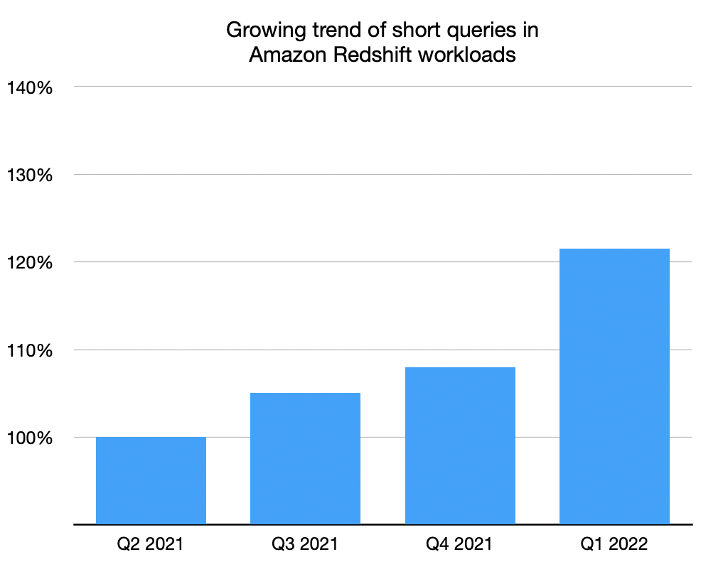
A specific metric we track is the percentage of runtime across all clusters that is spent on short-running queries (queries with runtime less than 1 second). Over the last year, we’ve seen a significant increase in short query workloads in the Amazon Redshift fleet, as shown in the following chart.

As we started to look deeper into how Amazon Redshift ran these kinds of workloads, we discovered several opportunities to optimize performance to give you even better throughput on short queries:

  • We significantly reduced Amazon Redshift’s query-planning overhead. Even though this isn’t large, it can be a significant portion of the runtime of short queries.
  • We improved the performance of several core components for situations where many concurrent processes contend for the same resources. This further reduced our query overhead.
  • We made improvements that allowed Amazon Redshift to more efficiently burst these short queries to concurrency scaling clusters to improve query parallelism.

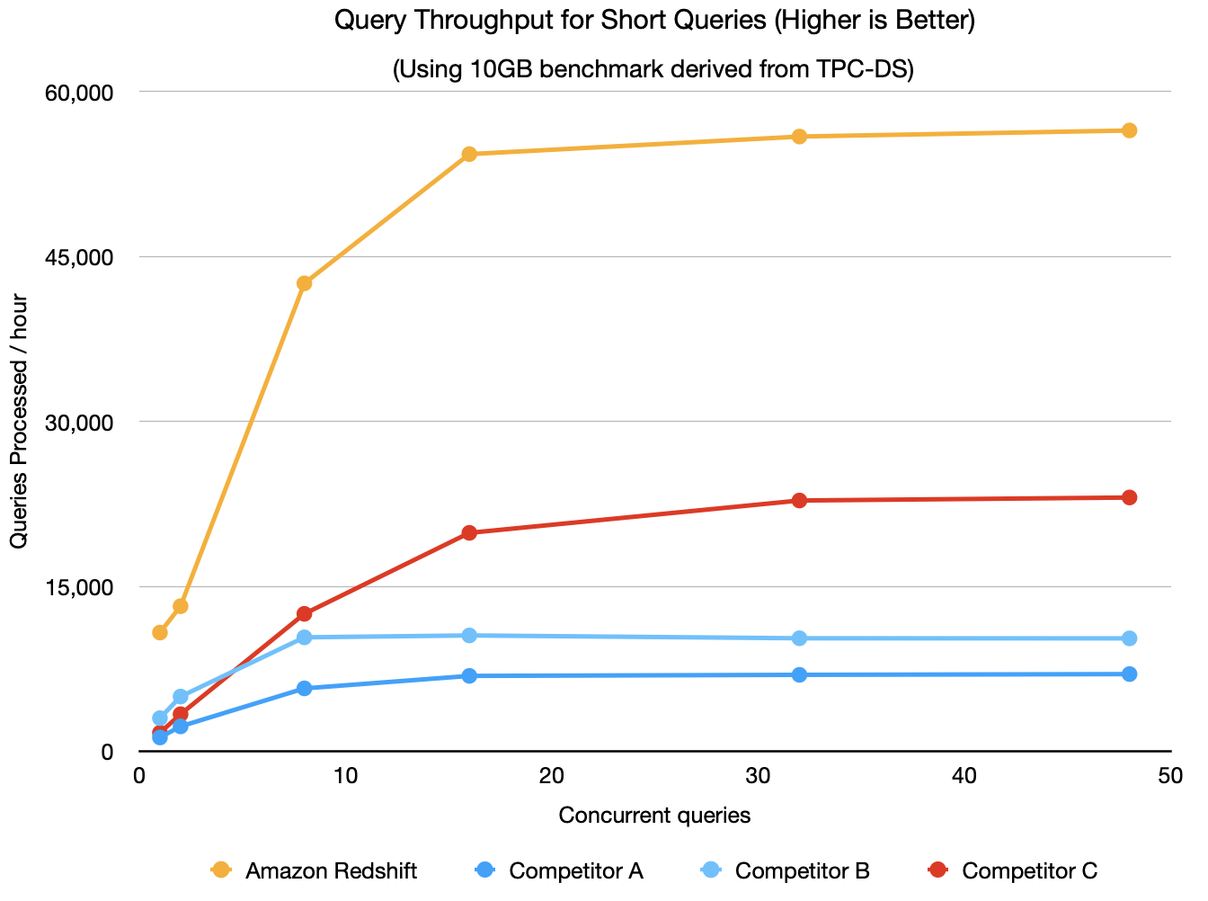
To see where Amazon Redshift stood after making these engineering improvements, we ran an internal test using the Cloud Data Warehouse Benchmark derived from TPC-DS (see a later section of this post for more details on the benchmark, which is available in GitHub). To simulate a high-concurrency, low-latency workload, we used a small 10 GB dataset so that all queries ran in a few seconds or less. We also ran the same benchmark against several other cloud data warehouses. We didn’t enable auto scaling features such as concurrency scaling on Amazon Redshift for this test because not all data warehouses support it. We used an ra3.4xlarge Amazon Redshift cluster, and sized all other warehouses to the closest matching price-equivalent configuration using on-demand pricing. Based on this configuration, we found that Amazon Redshift can deliver up to 8x better performance on analytics applications that predominantly required short queries with low latency and high concurrency, as shown in the following chart.

With Concurrency Scaling on Amazon Redshift, throughput can be seamlessly and automatically scaled to additional Amazon Redshift clusters as user concurrency grows. We increasingly see customers using Amazon Redshift to build such analytics applications based on our telemetry data.

This is just a small peek into the behind-the-scenes engineering improvements our team is continually making to help you improve performance and save costs using a data-driven approach.

New features improving price-performance

With the constantly evolving data landscape, customers want high-performance data warehouses that continue to launch new capabilities to deliver the best performance at scale while keeping costs low for all workloads and applications. We have continued to add features that improve Amazon Redshift’s price-performance out of the box at no additional cost to you, allowing you to solve business problems at any scale. These features include the use of best-in-class hardware through the AWS Nitro System, hardware acceleration with AQUA, auto-rewriting queries so that they run faster using materialized views, Automatic Table Optimization (ATO) for schema optimization, Automatic Workload Management (WLM) to offer dynamic concurrency and optimize resource utilization, short query acceleration, automatic materialized views, vectorization and single instruction/multiple data (SIMD) processing, and much more. Amazon Redshift has evolved to become a self-learning, self-tuning data warehouse, abstracting away the performance management effort needed so you can focus on high-value activities like building analytics applications.

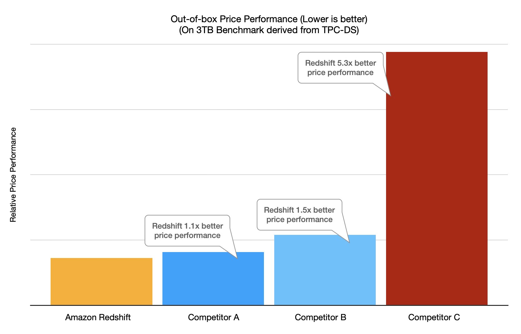
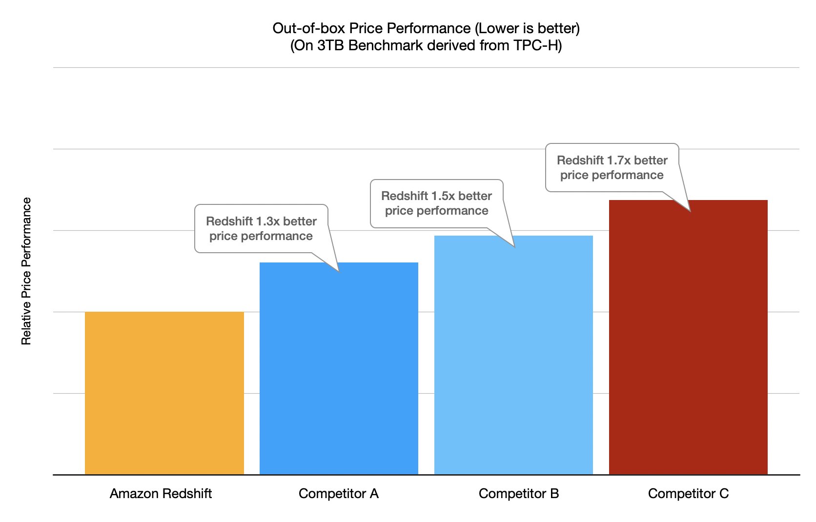
To validate the impact of the latest Amazon Redshift performance enhancements, we ran price-performance benchmarks comparing Amazon Redshift with other cloud data warehouses. For these tests, we ran both a TPC-DS-derived benchmark and a TPC-H-derived benchmark using a 10-node ra3.4xlarge Amazon Redshift cluster. To run the tests on other data warehouses, we chose warehouse sizes that most closely matched the Amazon Redshift cluster in price ($32.60 per hour), using published on-demand pricing for all data warehouses. Because Amazon Redshift is an auto-tuning warehouse, all tests are “out of the box,” meaning no manual tunings or special database configurations are applied—the clusters are launched and the benchmark is run. Price-performance is then calculated as cost per hour (USD) times the benchmark runtime in hours, which is equivalent to the cost to run the benchmark.

For both the TPC-DS-derived and TPC-H-derived tests, we find that Amazon Redshift consistently delivers the best price-performance. The following chart shows the results for the TPC-DS-derived benchmark.

The following chart shows the results for the TPC-H-derived benchmark.

Although these benchmarks reaffirm Amazon Redshift’s price-performance leadership, we always encourage you to try Amazon Redshift using your own proof-of-concept workloads as the best way to see how Amazon Redshift can meet your data needs.

Find the best price-performance for your workloads

The benchmarks used in this post are derived from the industry-standard TPC-DS and TPC-H benchmarks, and have the following characteristics:

  • The schema and data are used unmodified from TPC-DS and TPC-H.
  • The queries are used unmodified from TPC-DS and TPC-H. TPC-approved query variants are used for a warehouse if the warehouse doesn’t support the SQL dialect of the default TPC-DS or TPC-H query.
  • The test includes only the 99 TPC-DS and 22 TPC-H SELECT queries. It doesn’t include maintenance and throughput steps.
  • Three power runs (single stream) were run with query parameters generated using the default random seed of the TPC-DS and TPC-H kits.
  • The primary metric of total query runtime is used when calculating price-performance. The runtime is taken as the best of the three runs.
  • Price-performance is calculated as cost per hour (USD) times the benchmark runtime in hours, which is equivalent to cost to run the benchmark. Published on-demand pricing is used for all data warehouses.

We call this benchmark the Cloud Data Warehouse Benchmark, and you can easily reproduce the preceding benchmark results using the scripts, queries, and data available on GitHub. It is derived from the TPC-DS and TPC-H benchmarks as described earlier, and as such is not comparable to published TPC-DS or TPC-H results, because the results of our tests don’t comply with the specification.

Each workload has unique characteristics, so if you’re just getting started, a proof of concept is the best way to understand how Amazon Redshift performs for your requirements. When running your own proof of concept, it’s important to focus on the right metrics—query throughput (number of queries per hour) and price-performance. You can make a data-driven decision by running a proof of concept on your own or with assistance from AWS or a system integration and consulting partner.

Conclusion

This post discussed the analytic workload trends we’re seeing from Amazon Redshift customers, new capabilities we have launched to improve Amazon Redshift’s price-performance, and the results from the latest benchmarks.

If you’re an existing Amazon Redshift customer, connect with us for a free optimization session and briefing on the new features announced at AWS re:Invent 2021. To stay up to date with the latest developments in Amazon Redshift, follow the What’s New in Amazon Redshift feed.


About the Authors

Stefan Gromoll is a Senior Performance Engineer with Amazon Redshift where he is responsible for measuring and improving Redshift performance. In his spare time, he enjoys cooking, playing with his three boys, and chopping firewood.

Ravi Animi is a Senior Product Management leader in the Redshift Team and manages several functional areas of the Amazon Redshift cloud data warehouse service including performance, spatial analytics, streaming ingestion and migration strategies. He has experience with relational databases, multi-dimensional databases, IoT technologies, storage and compute infrastructure services and more recently as a startup founder using AI/deep learning, computer vision, and robotics.

Florian Wende is a Performance Engineer with Amazon Redshift.

How to protect HMACs inside AWS KMS

Post Syndicated from Jeremy Stieglitz original https://aws.amazon.com/blogs/security/how-to-protect-hmacs-inside-aws-kms/

Today AWS Key Management Service (AWS KMS) is introducing new APIs to generate and verify hash-based message authentication codes (HMACs) using the Federal Information Processing Standard (FIPS) 140-2 validated hardware security modules (HSMs) in AWS KMS. HMACs are a powerful cryptographic building block that incorporate secret key material in a hash function to create a unique, keyed message authentication code.

In this post, you will learn the basics of the HMAC algorithm as a cryptographic building block, including how HMACs are used. In the second part of this post, you will see a few real-world use cases that show an application builder’s perspective on using the AWS KMS HMAC APIs.

HMACs provide a fast way to tokenize or sign data such as web API requests, credit cards, bank routing information, or personally identifiable information (PII).They are commonly used in several internet standards and communication protocols such as JSON Web Tokens (JWT), and are even an important security component for how you sign AWS API requests.

HMAC as a cryptographic building block

You can consider an HMAC, sometimes referred to as a keyed hash, to be a combination function that fuses the following elements:

  • A standard hash function such as SHA-256 to produce a message authentication code (MAC).
  • A secret key that binds this MAC to that key’s unique value.

Combining these two elements creates a unique, authenticated version of the digest of a message. Because the HMAC construction allows interchangeable hash functions as well as different secret key sizes, one of the benefits of HMACs is the easy replaceability of the underlying hash function (in case faster or more secure hash functions are required), as well as the ability to add more security by lengthening the size of the secret key used in the HMAC over time. The AWS KMS HMAC API is launching with support for SHA-224, SHA-256, SHA-384, and SHA-512 algorithms to provide a good balance of key sizes and performance trade-offs in the implementation. For more information about HMAC algorithms supported by AWS KMS, see HMAC keys in AWS KMS in the AWS KMS Developer Guide.

HMACs offer two distinct benefits:

  1. Message integrity: As with all hash functions, the output of an HMAC will result in precisely one unique digest of the message’s content. If there is any change to the data object (for example you modify the purchase price in a contract by just one digit: from “$350,000” to “$950,000”), then the verification of the original digest will fail.
  2. Message authenticity: What distinguishes HMAC from other hash methods is the use of a secret key to provide message authenticity. Only message hashes that were created with the specific secret key material will produce the same HMAC output. This dependence on secret key material ensures that no third party can substitute their own message content and create a valid HMAC without the intended verifier detecting the change.

HMAC in the real world

HMACs have widespread applications and industry adoption because they are fast, high performance, and simple to use. HMACs are particularly popular in the JSON Web Token (JWT) open standard as a means of securing web applications, and have replaced older technologies such as cookies and sessions. In fact, Amazon implements a custom authentication scheme, Signature Version 4 (SigV4), to sign AWS API requests based on a keyed-HMAC. To authenticate a request, you first concatenate selected elements of the request to form a string. You then use your AWS secret key material to calculate the HMAC of that string. Informally, this process is called signing the request, and the output of the HMAC algorithm is informally known as the signature, because it simulates the security properties of a real signature in that it represents your identity and your intent.

Advantages of using HMACs in AWS KMS

AWS KMS HMAC APIs provide several advantages over implementing HMACs in application software because the key material for the HMACs is generated in AWS KMS hardware security modules (HSMs) that are certified under the FIPS 140-2 program and never leave AWS KMS unencrypted. In addition, the HMAC keys in AWS KMS can be managed with the same access control mechanisms and auditing features that AWS KMS provides on all AWS KMS keys. These security controls ensure that any HMAC created in AWS KMS can only ever be verified in AWS KMS using the same KMS key. Lastly, the HMAC keys and the HMAC algorithms that AWS KMS uses conform to industry standards defined in RFC 2104 HMAC: Keyed-Hashing for Message Authentication.

Use HMAC keys in AWS KMS to create JSON Web Tokens

The JSON Web Token (JWT) open standard is a common use of HMAC. The standard defines a portable and secure means to communicate a set of statements, known as claims, between parties. HMAC is useful for applications that need an authorization mechanism, in which claims are validated to determine whether an identity has permission to perform some action. Such an application can only work if a validator can trust the integrity of claims in a JWT. Signing JWTs with an HMAC is one way to assert their integrity. Verifiers with access to an HMAC key can cryptographically assert that the claims and signature of a JWT were produced by an issuer using the same key.

This section will walk you through an example of how you can use HMAC keys from AWS KMS to sign JWTs. The example uses the AWS SDK for Python (Boto3) and implements simple JWT encoding and decoding operations. This example shows the ease with which you can integrate HMAC keys in AWS KMS into your JWT application, even if your application is in another language or uses a more formal JWT library.

Create an HMAC key in AWS KMS

Begin by creating an HMAC key in AWS KMS. You can use the AWS KMS console or call the CreateKey API action. The following example shows creation of a 256-bit HMAC key:

import boto3

kms = boto3.client('kms')

# Use CreateKey API to create a 256-bit key for HMAC
key_id = kms.create_key(
	KeySpec='HMAC_256',
	KeyUsage='GENERATE_VERIFY_MAC'
)['KeyMetadata']['KeyId']

Use the HMAC key to encode a signed JWT

Next, you use the HMAC key to encode a signed JWT. There are three components to a JWT token: the set of claims, header, and signature. The claims are the very application-specific statements to be authenticated. The header describes how the JWT is signed. Lastly, the MAC (signature) is the output of applying the header’s described operation to the message (the combination of the claims and header). All these are packed into a URL-safe string according to the JWT standard.

The following example uses the previously created HMAC key in AWS KMS within the construction of a JWT. The example’s claims simply consist of a small claim and an issuance timestamp. The header contains key ID of the HMAC key and the name of the HMAC algorithm used. Note that HS256 is the JWT convention used to represent HMAC with SHA-256 digest. You can generate the MAC using the new GenerateMac API action in AWS KMS.

import base64
import json
import time

def base64_url_encode(data):
	return base64.b64encode(data, b'-_').rstrip(b'=')

# Payload contains simple claim and an issuance timestamp
payload = json.dumps({
	"does_kms_support_hmac": "yes",
	"iat": int(time.time())
}).encode("utf8")

# Header describes the algorithm and AWS KMS key ID to be used for signing
header = json.dumps({
	"typ": "JWT",
	"alg": "HS256",
	"kid": key_id #This key_id is from the “Create an HMAC key in AWS KMS” #example. The “Verify the signed JWT” example will later #assert that the input header has the same value of the #key_id 
}).encode("utf8")

# Message to sign is of form <header_b64>.<payload_b64>
message = base64_url_encode(header) + b'.' + base64_url_encode(payload)

# Generate MAC using GenerateMac API of AWS KMS
MAC = kms.generate_mac(
	KeyId=key_id, #This key_id is from the “Create an HMAC key in AWS KMS” 
				 #example
	MacAlgorithm='HMAC_SHA_256',
	Message=message
)['Mac']

# Form JWT token of form <header_b64>.<payload_b64>.<mac_b64>
jwt_token = message + b'.' + base64_url_encode(mac)

Verify the signed JWT

Now that you have a signed JWT, you can verify it using the same KMS HMAC key. The example below uses the new VerifyMac API action to validate the MAC (signature) of the JWT. If the MAC is invalid, AWS KMS returns an error response and the AWS SDK throws an exception. If the MAC is valid, the request succeeds and the application can continue to do further processing on the token and its claims.

def base64_url_decode(data):
	return base64.b64decode(data + b'=' * (4 - len(data) % 4), b'-_')

# Parse out encoded header, payload, and MAC from the token
message, mac_b64 = jwt_token.rsplit(b'.', 1)
header_b64, payload_b64 = message.rsplit(b'.', 1)

# Decode header and verify its contents match expectations
header_map = json.loads(base64_url_decode(header_b64).decode("utf8"))
assert header_map == {
	"typ": "JWT",
	"alg": "HS256",
	"kid": key_id #This key_id is from the “Create an HMAC key in AWS KMS” 
				 #example
}

# Verify the MAC using VerifyMac API of AWS KMS. # If the verification fails, this will throw an error.
kms.verify_mac(
	KeyId=key_id, #This key_id is from the “Create an HMAC key in AWS KMS” 
				 #example
	MacAlgorithm='HMAC_SHA_256',
	Message=message,
	Mac=base64_url_decode(mac_b64)
)

# Decode payload for use application-specific validation/processing
payload_map = json.loads(base64_url_decode(payload_b64).decode("utf8"))

Create separate roles to control who has access to generate HMACs and who has access to validate HMACs

It’s often helpful to have separate JWT creators and validators so that you can distinguish between the roles that are allowed to create tokens and the roles that are allowed to verify tokens. HMAC signatures performed outside of AWS-KMS don’t work well for this because you can’t isolate creators and verifiers if they both must have a copy of the same key. However, this is not an issue for HMAC keys in AWS KMS. You can use key policies to separate out who has permission to ask AWS KMS to generate HMACs and who has permission to ask AWS KMS to validate. Each party uses their own unique access keys to access the HMAC key in AWS KMS. Only HSMs in AWS KMS will ever have access to the actual key material. See the following example key policy statements that separate out GenerateMac and VerifyMac permissions:

{
	"Id": "example-jwt-policy",
	"Version": "2012-10-17",
	"Statement": [
		{
			"Sid": "Allow use of the key for creating JWTs",
			"Effect": "Allow",
			"Principal": {
				"AWS": "arn:aws:iam::111122223333:role/JwtProducer"
			},
			"Action": [
				"kms:GenerateMac"
			],
			"Resource": "*"
		},
		{
			"Sid": "Allow use of the key for validating JWTs",
			"Effect": "Allow",
			"Principal": {
				"AWS": "arn:aws:iam::111122223333:role/JwtConsumer"
			},
			"Action": [
				"kms:VerifyMac"
			],
			"Resource": "*"
		}
	]
}

Conclusion

In this post, you learned about the new HMAC APIs in AWS KMS (GenerateMac and VerifyMac). These APIs complement existing AWS KMS cryptographic operations: symmetric key encryption, asymmetric key encryption and signing, and data key creation and key enveloping. You can use HMACs for JWTs, tokenization, URL and API signing, as a key derivation function (KDF), as well as in new designs that we haven’t even thought of yet. To learn more about HMAC functionality and design, see HMAC keys in AWS KMS in the AWS KMS Developer Guide.

If you have feedback about this post, submit comments in the Comments section below. If you have questions about this post, start a new thread on the KMS re:Post or contact AWS Support.
Want more AWS Security news? Follow us on Twitter.

Author

Jeremy Stieglitz

Jeremy is the Principal Product Manager for AWS Key Management Service (KMS) where he drives global product strategy and roadmap for AWS KMS. Jeremy has more than 20 years of experience defining new products and platforms, launching and scaling cryptography solutions, and driving end-to-end product strategies. Jeremy is the author or co-author of 23 patents in network security, user authentication and network automation and control.

Author

Peter Zieske

Peter is a Senior Software Developer on the AWS Key Management Service team, where he works on developing features on the service-side front-end. Outside of work, he enjoys building with LEGO, gaming, and spending time with family.

Undetectable Backdoors in Machine-Learning Models

Post Syndicated from Bruce Schneier original https://www.schneier.com/blog/archives/2022/04/undetectable-backdoors-in-machine-learning-models.html

New paper: “Planting Undetectable Backdoors in Machine Learning Models“:

Abstract: Given the computational cost and technical expertise required to train machine learning models, users may delegate the task of learning to a service provider. We show how a malicious learner can plant an undetectable backdoor into a classifier. On the surface, such a backdoored classifier behaves normally, but in reality, the learner maintains a mechanism for changing the classification of any input, with only a slight perturbation. Importantly, without the appropriate “backdoor key”, the mechanism is hidden and cannot be detected by any computationally-bounded observer. We demonstrate two frameworks for planting undetectable backdoors, with incomparable guarantees.

First, we show how to plant a backdoor in any model, using digital signature schemes. The construction guarantees that given black-box access to the original model and the backdoored version, it is computationally infeasible to find even a single input where they differ. This property implies that the backdoored model has generalization error comparable with the original model. Second, we demonstrate how to insert undetectable backdoors in models trained using the Random Fourier Features (RFF) learning paradigm or in Random ReLU networks. In this construction, undetectability holds against powerful white-box distinguishers: given a complete description of the network and the training data, no efficient distinguisher can guess whether the model is “clean” or contains a backdoor.

Our construction of undetectable backdoors also sheds light on the related issue of robustness to adversarial examples. In particular, our construction can produce a classifier that is indistinguishable from an “adversarially robust” classifier, but where every input has an adversarial example! In summary, the existence of undetectable backdoors represent a significant theoretical roadblock to certifying adversarial robustness.

EDITED TO ADD (4/20): Cory Doctorow wrote about this as well.

What’s New in InsightVM and Nexpose: Q1 2022 in Review

Post Syndicated from Roshnee Mistry Shah original https://blog.rapid7.com/2022/04/19/whats-new-in-insightvm-and-nexpose-q1-2022-in-review/

What's New in InsightVM and Nexpose: Q1 2022 in Review

The world of cybersecurity never has a dull moment. While we are still recovering from the aftermath of Log4Shell, the recent ContiLeaks exposed multiple vulnerabilities that have been exploited by the Conti ransomware group. It’s critical for your team to identify the risk posed by such vulnerabilities and implement necessary remediation measures. As you will see, the product updates our vulnerability management (VM) team has made to InsightVM and Nexpose in the last quarter will empower you to stay in charge — not the vulnerabilities.

But that’s not all we’ve improved on. We’ve increased the scope of vulnerabilities tracked by incorporating CISA’s known exploited vulnerabilities (KEV) in the Threat Feed, usability enhancements, targeted reporting and scanning, and Log4Shell mitigation checks. And we’ve released our annual Vulnerability Intelligence Report to help you make sense of the vulns that impacted us last year and understand the trends that we will all be facing this year. Our team also offers practical guidance to help the security teams better protect themselves.

Let’s dive into the key feature releases and updates on the vulnerability management front for Q1 2022.

CISA’s KEV list: Detect, prioritize, and meet regulatory compliance

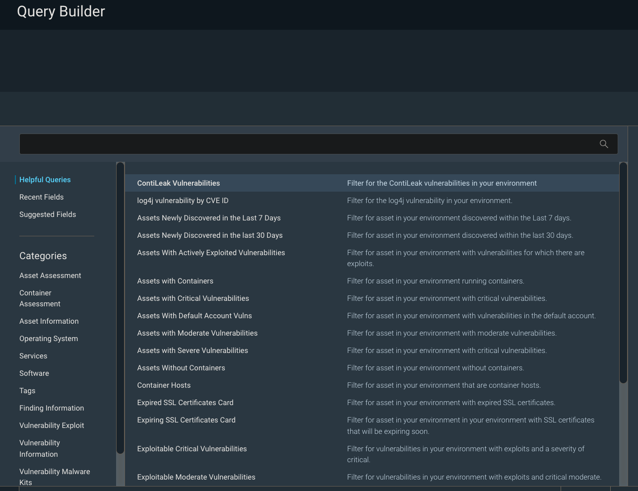
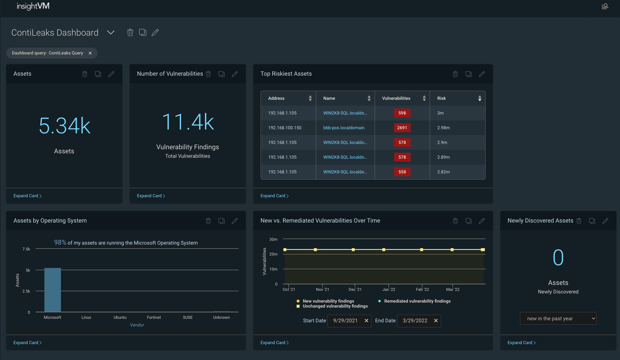
[InsightVM] ContiLeaks Helpful Query to easily detect ContiLeaks vulns and ensure compliance

CISA’s KEV catalog is part of the agency’s binding operative directive that has reporting requirements for federal agencies and civilian contractors. The recent ContiLeaks revealed over 30 vulns that are now a part of CISA’s KEV. While users could always build a query in IVM to identify these vulns, doing so is time-consuming and can be prone to error. The ContiLeaks Helpful Query takes out the manual effort  and lets customers easily locate 30+ ContiLeaks vulnerabilities in their environments. When the query is loaded into our Specific Vulnerability Dashboard template, it can give an at-a-glance view of the company’s risk posture as it relates to the Conti threat. In addition to helping customers identify the exploited vulnerabilities in their environment, the update will also help them stay within the bounds of CISA’s operative directive.

What's New in InsightVM and Nexpose: Q1 2022 in Review

What's New in InsightVM and Nexpose: Q1 2022 in Review

[InsightVM] Threat feed dashboard now includes CISA’s KEV catalog

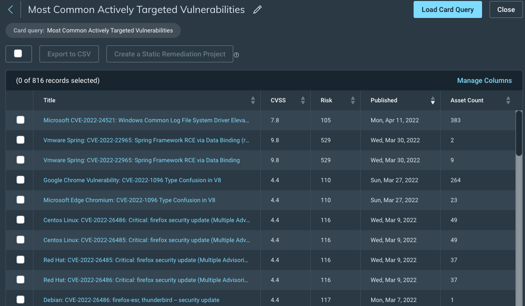
While we are on the topic of CISA, you will be excited to learn that we have expanded the scope of vulnerabilities tracked to incorporate CISA’s KEV catalog in the InsightVM Threat Feed Dashboard, including the Assets With Actively Targeted Vulnerabilities card and the Most Common Actively Targeted Vulnerabilities card. The CISA inclusion makes it easy to see how exposed your organization is to active threats and inform prioritization decisions around remediation efforts.

We have also added a new “CISA KEV (known exploited vulnerability)” vulnerability category to allow for more targeted scanning (i.e. scanning the environment for CISA KEV entries only). You can also use the CISA KEV category to filter scan reports.

What's New in InsightVM and Nexpose: Q1 2022 in Review

Improvements to credentials

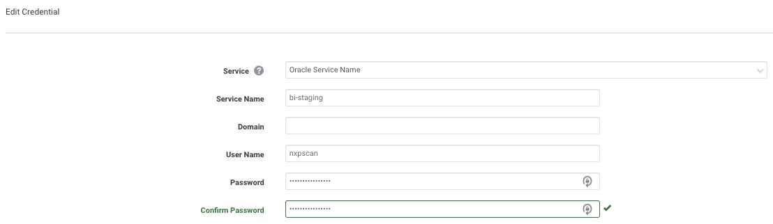
[Insight VM and Nexpose] A new credential type to support scanning Oracle Databases by Service Name

InsightVM and Nexpose customers have always been able to scan Oracle databases using SIDs (system identifiers) but were previously unable to provide a Service Name in the credential. This meant a gap in visibility for Oracle databases that could only be accessed via their Service Name. We were not happy with this limitation. Now, you now configure Oracle Database scans to specify a Service Name instead of an SID (you can still use the SID, if you want!) when authenticating. You now have the visibility into a wider range of deployment configurations of Oracle Database and the ability to configure scan using Service Name or SID.

What's New in InsightVM and Nexpose: Q1 2022 in Review

[Insight VM and Nexpose] Automatic Scan Assistant credentials generation

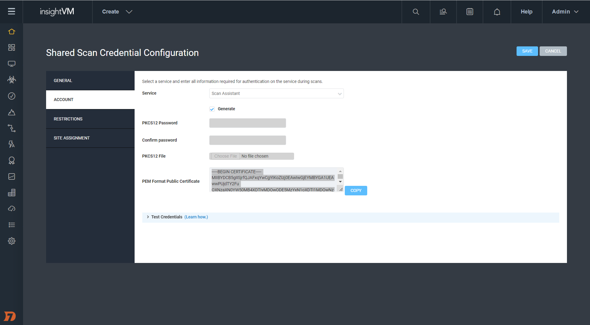
Last year, we introduced Scan Assistant, which alleviates the credential management (for Scan Engine) burden on vulnerability management teams. For the Scan Assistant to communicate with the Scan Engine, it requires digital certificates to be manually created and deployed on both the target assets and the Nexpose / IVM Security Console. Manually creating the public / private key pair is a complex and error-prone process.

With this update, we are taking some more burden off the vulnerability management teams. You can now use the Shared Credentials management UI to automatically generate Scan Assistant credentials. This not only reduces the technical expertise and time required to manage Scan Assistant credentials but also makes for a user-friendly experience for you.

Learn more in our recent blog post on passwordless scanning.

What's New in InsightVM and Nexpose: Q1 2022 in Review

[Insight VM and Nexpose] Log4Shell mitigation checks

The product improvements list would be incomplete without an update on Log4Shell.

If you are vulnerable to Log4Shell, you can edit the JAR files on a system to take out the vulnerable code and thus not get exploited. However, it is difficult to keep a check on this manually. This update adds that extra capability to not only look at the version of Log4j that was present in your environment but also check if it has been mitigated — i.e., if the vulnerable code is removed.

Authenticated scans and Agent-based assessments can now determine whether the JNDILookup class removal mitigation for Log4Shell has been applied to Log4j JAR files on Windows systems. This will reduce the number of reports of the vulnerability on systems that are not exploitable. We also added an Obsolete Software vulnerability check for Log4j 1.x, which will let you find obsolete versions of Log4j in your environment.

Stay in charge

As always, we hope these updates will make it easier for you to stay ahead of vulnerabilities.

It almost felt like the quarter might end on a calm note, but then the world of cybersecurity never has a dull moment. The end of the quarter saw Spring4Shell, another zero-day vulnerability in the Spring Core module of Spring Framework. Learn more about Rapid7 response to this vulnerability and how we are working around the clock to help our customers protect their own environments from Spring4Shell.

Additional reading:

NEVER MISS A BLOG

Get the latest stories, expertise, and news about security today.

Building SAML federation for Amazon OpenSearch Dashboards with Ping Identity

Post Syndicated from Raghavarao Sodabathina original https://aws.amazon.com/blogs/architecture/building-saml-federation-for-amazon-opensearch-dashboards-with-ping-identity/

Amazon OpenSearch is an open search and log analytics service, powered by the Apache Lucene search library.

In this blog post, we provide step-by-step guidance for SP-initiated SSO by showing how to set up a trial Ping Identity account. We’ll show how to build users and groups within your organization’s directory and enable SSO in OpenSearch Dashboards.

To use this feature, you must enable fine-grained access control. Rather than authenticating through Amazon Cognito or the internal user database, SAML authentication for OpenSearch Dashboards lets you use third-party identity providers to log in.

Ping Identity is an AWS Competency Partner, and the provider of the PingOne Cloud Platform is a multi-tenant Identity-as-a-Service (IDaaS) platform. Ping Identity supports both service provider (SP)-initiated and identity provider (IdP)-initiated SSO.

Overview of Ping Identity SAML authenticated solution

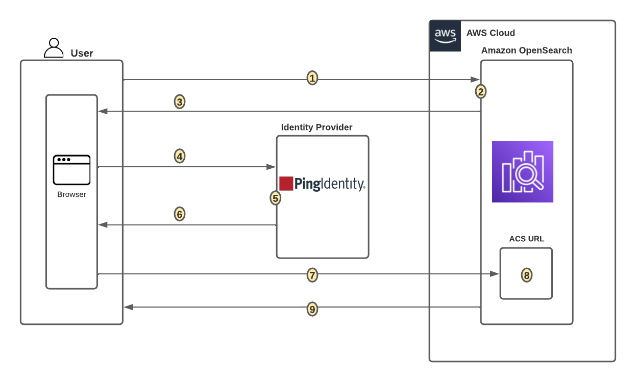
Figure 1 shows a sample architecture of a generic integrated solution between Ping Identity and OpenSearch Dashboards over SAML authentication.

SAML transactions between Amazon OpenSearch and Ping Identity

Figure 1. SAML transactions between Amazon OpenSearch and Ping Identity

The sign-in flow is as follows:

  1. User opens browser window and navigates to Amazon OpenSearch Dashboards
  2. Amazon OpenSearch generates SAML authentication request
  3. Amazon OpenSearch redirects request back to browser
  4. Browser redirects to Ping Identity URL
  5. Ping Identity parses SAML request, authenticates user, and generates SAML response
  6. Ping Identity returns encoded SAML response to browser
  7. Browser sends SAML response back to Amazon OpenSearch Assertion Consumer Service (ACS) URL
  8. ACS verifies SAML response
  9. User logs into Amazon OpenSearch domain

Prerequisites

For this walkthrough, you should have the following prerequisites:

  1. An AWS account
  2. A virtual private cloud (VPC)-based Amazon OpenSearch domain with fine-grained access control enabled
  3. Ping Identity account with user and a group
  4. A browser with network connectivity to Ping Identity, Amazon OpenSearch domain, and Amazon OpenSearch Dashboards.

The steps in this post are structured into the following sections:

  1. Identity provider (Ping Identity) setup
  2. Prepare Amazon OpenSearch for SAML configuration
  3. Identity provider (Ping Identity) SAML configuration
  4. Finish Amazon OpenSearch for SAML configuration
  5. Validation
  6. Cleanup

Identity provider (Ping Identity) setup

Step 1: Sign up for a Ping Identity account

  • Sign up for a Ping Identity account, then click on the Sign up button to complete your account setup.
  • If you already have an account with Ping Identity, login to your Ping Identity account.

Step 2: Create Population in Ping Identity

  • Choose Identities in the left menu and click Populations to proceed.
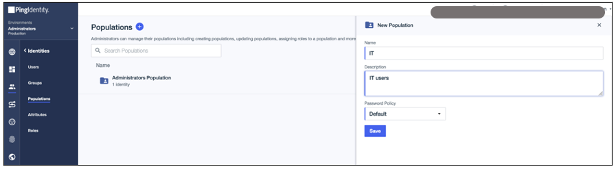
  • Click on the blue + button next to Populations, enter the name as IT, then click on the Save button (see Figure 2).
Creating population in Ping Identity

Figure 2. Creating population in Ping Identity

Step 3: Create a group in Ping Identity

  • Choose Groups from the left menu and click on the blue + button next to Groups. For this example, we will create a group called opensearch for Kibana access. Click on the Save button to complete the group creation.

Step 4: Create users in Ping Identity

  • Choose Users in left menu, then click the + Add User button.
  • Provide GIVEN NAME, FAMILY NAME, EMAIL ADDRESS, and choose Population as users, as created in Step 1. Choose your own USERNAME. Click on the SAVE button to create your user.
  • Add more users as needed.

Step 5: Assign role and group to users

  • Click on Identities/users in the left menu, and click on Users. Then click on the edit button for a particular user, as shown in Figure 3.
Assigning roles and groups to users in Ping Identity

Figure 3. Assigning roles and groups to users in Ping Identity

  • Click on the Edit button, click on + Add Role button, and click on the edit button to assign a role to the user.
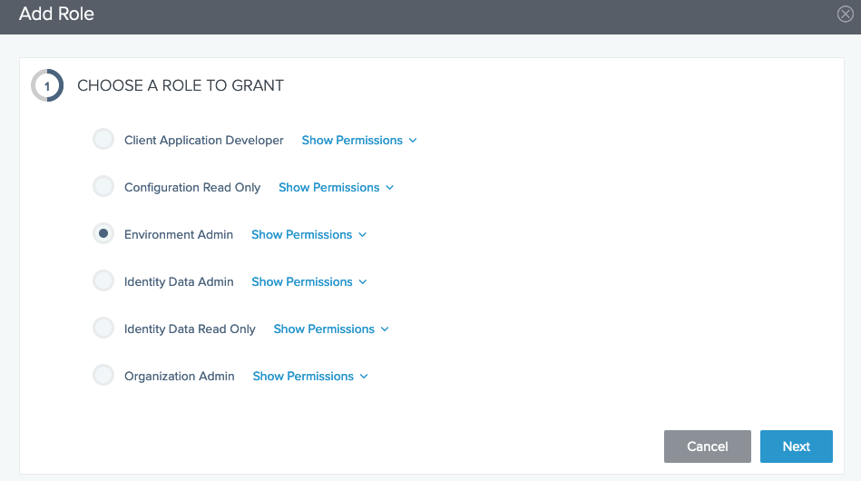
  • For this example, choose Environment Admin, as shown in Figure 4. You can choose different roles depending on your use case.
Assigning roles to users in Ping Identity

Figure 4. Assigning roles to users in Ping Identity

  • For this example, assign administrator responsibilities for our users. Click on Show Environments, and drag Administrators into the ADDED RESPONSIBILITES section. Then click on the Add Role button.
  • Add Group to users. Go to the Groups tab, search for the opensearch group created in Step 3. Click on the + button next to opensearch to add into group memberships.

Prepare Amazon OpenSearch for SAML configuration

Once the Amazon OpenSearch domain is up and running, we can proceed with configuration.

  • Under Actions, choose Edit security configuration, as shown in Figure 5.
Enabling Amazon OpenSearch security configuration for SAML

Figure 5. Enabling Amazon OpenSearch security configuration for SAML

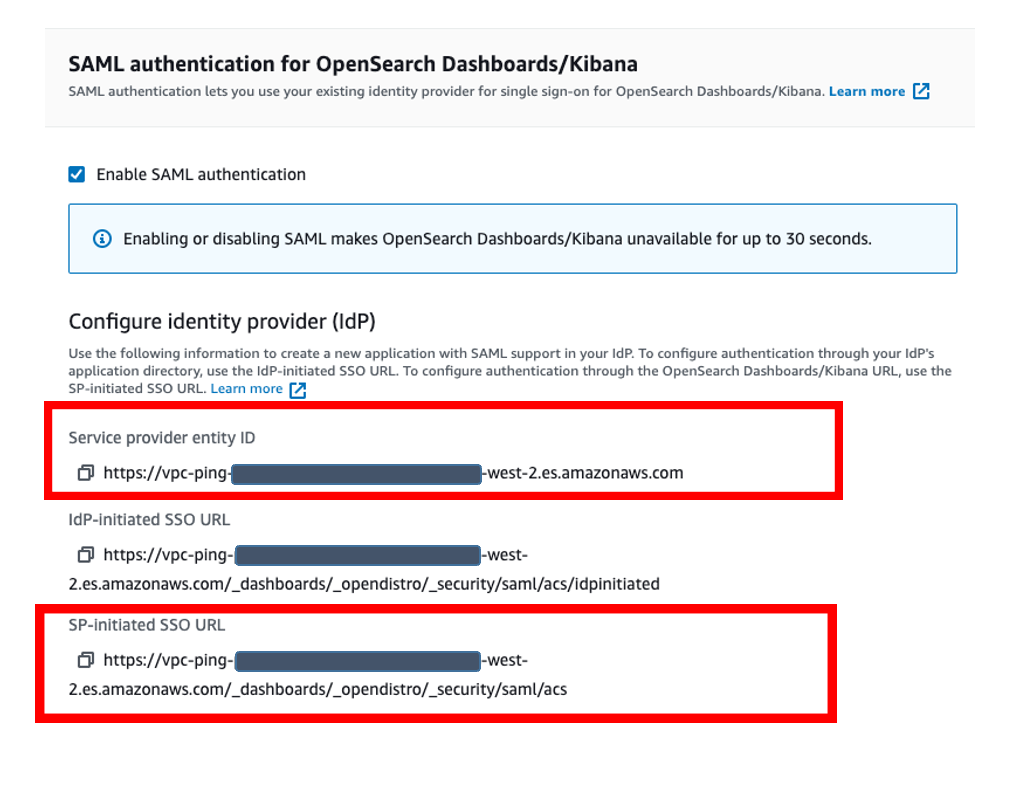
  • Under SAML authentication for OpenSearch Dashboards/Kibana, select Enable SAML authentication check box (Figure 6). When we enable SAML, it will create different URLs required for configuring SAML with your identity provider.
Amazon OpenSearch URLs for SAML configuration

Figure 6. Amazon OpenSearch URLs for SAML configuration

We will be using the Service Provider entity ID and SP-initiated SSO URL as highlighted in Figure 6 for Ping Identity SAML configuration. We will complete the rest of the Amazon OpenSearch SAML configuration after the Ping Identity SAML configuration.

Ping Identity SAML configuration

Go back to PingIdentity.com, and navigate to Connections on the left menu. Then select Applications, and click on Application +.

  • For this example, we are creating an application called “Kibana”
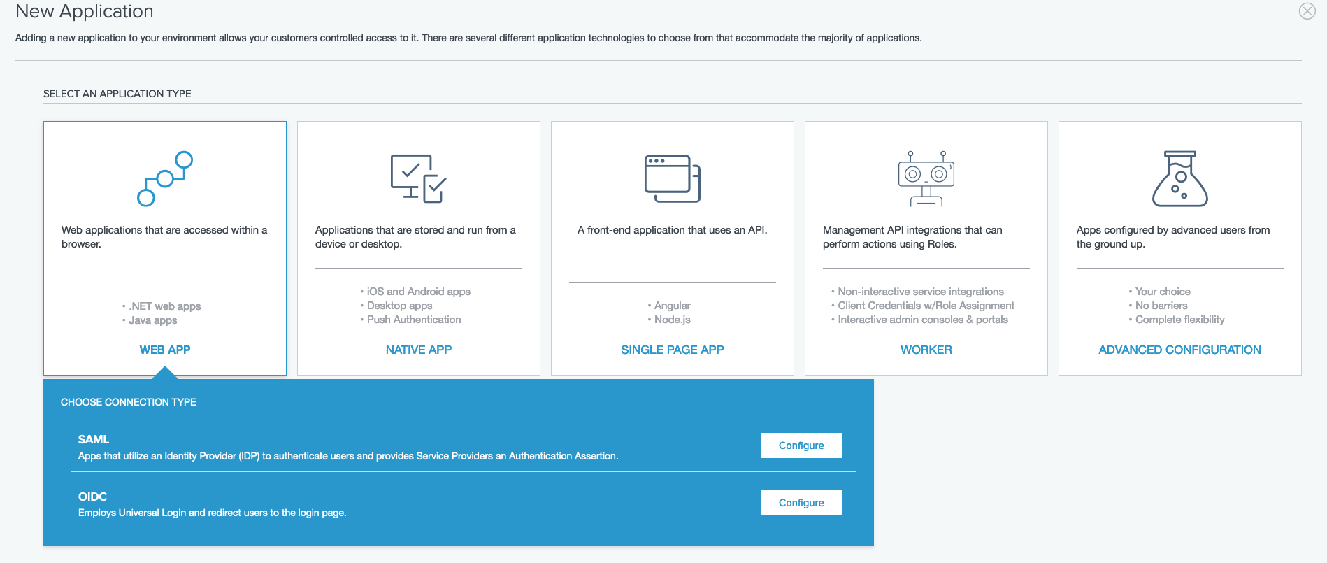
  • Select WEB APP as APPLICATION TYPE and CHOOSE CONNECTION TYPE as SAML, and click on Configure button to proceed as shown in Figure 7.
Configuring a new application in Ping Identity

Figure 7. Configuring a new application in Ping Identity

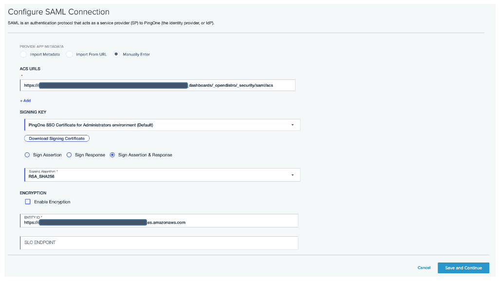
  • On the “Create App Profile” page, click on the Next button, and choose the “Manually Enter” option for PROVIDE APP METADATA. Enter the following under Configure SAML Connection section
    • ACS URL https://vpc-XXXXX-XXXXX-west-2.es.amazonaws.com/_dashboards/_opendistro/_security/saml/acs (SP-initiated SSO URL)
    • Choose Sign Assertion & Response under SIGNING KEY
    • ENTITY ID: https://vpc-XXXXX-XXXXX.us-west-2.es.amazonaws.com (Service provider entity ID)
    • ASSERTION VALIDITY DURATION (IN SECONDS) as 3600
    • Choose default options, then click on the Save and Continue button as shown in Figure 8
Configuring SAML connection in Ping Identity

Figure 8. Configuring SAML connection in Ping Identity

  • Enter the following under Configure Attribute Mapping, then click on Save and Close.
    • Set User ID to default
    • Click on +ADD ATTRIBUTE button to add following SAML attributes
      • OUTGOING VALUE: Group Names, SAML ATTRIBUTE: saml_group
      • OUTGOING VALUE: Username, SAML ATTRIBUTE: saml_username
  • Select the Policies tab and click on edit icon on the right.
  • Add the Single_Factor policy to the application, then click on Save.
  • Select the Access tab, add the opensearch group to the application, then click on Save to complete SAML configuration.
  • Finally, go to the Configuration tab, click on the Download Metadata button to download the Ping Identity metadata for the Amazon OpenSearch SAML configuration. Enable opensearch SAML application (Figure 9).
Downloading metadata in Ping Identity

Figure 9. Downloading metadata in Ping Identity

Amazon OpenSearch SAML configuration

  • Switch back to Amazon OpenSearch domain:
    • Navigate to the Amazon OpenSearch console.
    • Click on Actions, then click on Modify Security configuration.
    • Select the Enable SAML authentication check box.
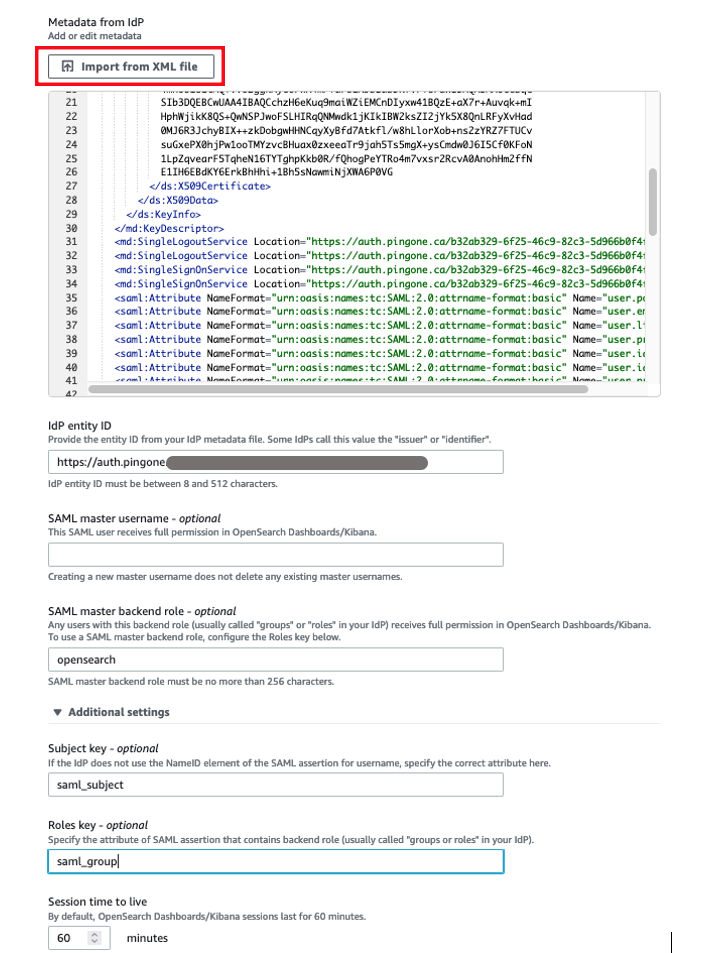
  • Under Import IdP metadata section:
    • Metadata from IdP: Import the Ping Identity identity provider metadata from the downloaded XML file, shown in Figure 10.
    • SAML master backend role: opensearch (Ping Identity group). Provide SAML backend role/group SAML assertion key for group SSO into Kibana.
Configuring Amazon OpenSearch SAML parameters

Figure 10. Configuring Amazon OpenSearch SAML parameters

  • Under Optional SAML settings:
    • Leave the Subject Key as saml_subject from Ping Identity SAML application attribute name.
    • Role key should be saml_group. You can view a sample assertion during the configuration process by tools like SAML-tracer. This can help you examine and troubleshoot the contents of real assertions.
    • Session time to live (mins): 60
  • Click on the Submit button to complete Amazon OpenSearch SAML configuration for Kibana. We have successfully completed SAML configuration and are now ready for testing.

Validating Access with Ping Identity Users

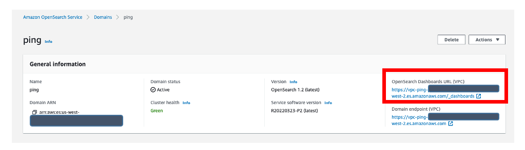
  • The OpenSearch Dashboards URL can be found in the Overview tab within “General Information” in the Amazon OpenSearch console (Figure 11). The first access to the OpenSearch Dashboards URL redirects you to the Ping Identity login screen.
Validating Ping Identity users access with Amazon OpenSearch

Figure 11. Validating Ping Identity users access with Amazon OpenSearch

  • If your OpenSearch domain is hosted within a private VPC, you will not be able to access OpenSearch Dashboards over public internet. But you can still use SAML as long as your browser can communicate with both your OpenSearch cluster and your identity provider.
  • You can create a Mac or Windows EC2 instance within the same VPC and access Amazon OpenSearch Dashboards from an EC2 instance’s web browser to validate your SAML configuration. Or you can access your Amazon OpenSearch Dashboards through Site-to-Site VPN if you are trying to access it from your on-premises environment.
  • Now copy and paste the OpenSearch Dashboards URL in your browser, and enter user credentials.
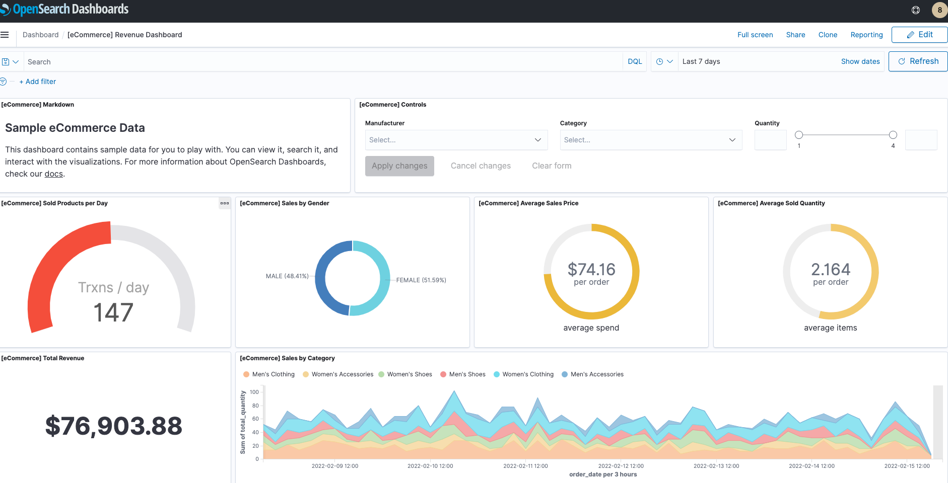
  • After successful login, you will be redirected into the OpenSearch Dashboards home page. Explore our sample data and visualizations in OpenSearch Dashboards, as shown in Figure 12.
SAML authenticated Amazon OpenSearch Dashboards

Figure 12. SAML authenticated Amazon OpenSearch Dashboards

  • You have successfully federated Amazon OpenSearch Dashboards with Ping Identity as an identity provider. You can connect OpenSearch Dashboards by using your Ping Identity credentials.

Cleaning up

After you test out this solution, remember to delete all the resources you created to avoid incurring future charges. Refer to these links:

Conclusion

In this blog post, we have demonstrated how to set up Ping Identity as an identity provider over SAML authentication for Amazon OpenSearch Dashboards access. With this solution, you now have an OpenSearch Dashboard that uses Ping Identity as the custom identity provider for your users. This reduces the customer login process to one set of credentials and improves employee productivity.

Get started by checking the Amazon OpenSearch Developer Guide, which provides guidance on how to build applications using Amazon OpenSearch for your operational analytics.

Automate notifications on Slack for Amazon Redshift query monitoring rule violations

Post Syndicated from Dipankar Kushari original https://aws.amazon.com/blogs/big-data/automate-notifications-on-slack-for-amazon-redshift-query-monitoring-rule-violation/

In this post, we walk you through how to set up automatic notifications of query monitoring rule (QMR) violations in Amazon Redshift to a Slack channel, so that Amazon Redshift users can take timely action.

Amazon Redshift is a fully managed, petabyte-scale data warehouse service in the cloud. With Amazon Redshift, you can analyze your data to derive holistic insights about your business and your customers. One of the challenges is to protect the data warehouse workload from poorly written queries that can consume significant resources. Amazon Redshift query monitoring rules are a feature of workload management (WLM) that allow automatic handling of poorly written queries. Rules that are applied to a WLM queue allow queries to be logged, canceled, hopped (only available with manual WLM), or to change priority (only available with automatic WLM). The reason to use QMRs is to protect against wasteful use of the cluster. You can also use these rules to log resource-intensive queries, which provides the opportunity to establish governance for ad hoc workloads.

The Amazon Redshift cluster automatically collects query monitoring rules metrics. This convenient mechanism lets you view attributes like the following:

  • Query runtime, in seconds
  • Query return row count
  • The CPU time for a SQL statement

It also makes Amazon Redshift Spectrum metrics available, such as the number of Redshift Spectrum rows and MBs scanned by a query.

When a query violates a QMR, Amazon Redshift logs the violation into the STL_WLM_RULE_ACTION system view. If the action is aborted for the queries that violate a QMR, end-users see an error that indicates query failure due to violation of QMRs. We recommend that administrative team members periodically examine violations listed in the STL_WLM_RULE_ACTION table and coach the involved end-users on how to avoid future rule violations.

Alternately, a centralized team, using a Slack channel for collaboration and monitoring, can configure Amazon Redshift events and alarms to be sent to their channel, so that they can take timely action. In the following sections, we walk you through how to set up automatic notifications of QMR violations to a Slack channel through the use of Slack events and alarms. This allows Amazon Redshift users to be notified and take timely actions without the need to query the system view.

Solution overview

To demonstrate how you can receive automatic notification to a Slack channel for QMR violation, we have designed the following architecture. As shown in the following diagram, we have mixed workload extract, transform, and load (ETL), business intelligence (BI) dashboards, and analytics applications that are powered by an Amazon Redshift cluster. The solution relies on AWS Lambda and Amazon Simple Notification Service (Amazon SNS) to send notifications of Amazon Redshift QMR violations to Slack.

To implement this solution, you create an Amazon Redshift cluster and attach a custom defined parameter group.

Amazon Redshift provides one default parameter group for each parameter group family. The default parameter group has preset values for each of its parameters, and it can’t be modified. If you want to use different parameter values than the default parameter group, you must create a custom parameter group and then associate your cluster with it.

In the parameter group, you can use automatic WLM and define a few workload queues, such as a queue for processing ETL workloads and a reporting queue for user queries. You can name the default queue adhoc. With automatic WLM, Amazon Redshift determines the optimal concurrency and memory allocation for each query that is running in each queue.

For each workload queue, you can define one or more QMRs. For example, you can create a rule to abort a user query if it runs for more than 300 seconds or returns more than 1 billion rows. Similarly, you can create a rule to log a Redshift Spectrum query that scans more than 100 MB.

The Amazon Redshift WLM evaluates metrics every 10 seconds. It records details about actions that result from QMR violation that is associated with user-defined queues in the STL_WLM_RULE_ACTION system table. In this solution, a Lambda function is scheduled to monitor the STL_WLM_RULE_ACTION system table every few minutes. When the function is invoked, if it finds a new entry, it publishes a detailed message to an SNS topic. A second Lambda function, created as the target subscriber to the SNS topic, is invoked whenever any message is published to the SNS topic. This second function invokes a pre-created Slack webhook, which sends the message that was received through the SNS topic to the Slack channel of your choice. (For more information on publishing messages by using Slack webhooks, see Sending messages using incoming webhooks.)

To summarize, the solution involves the following steps:

  1. Create an Amazon Redshift custom parameter group and add workload queues.
  2. Configure query monitoring rules.
  3. Attach the custom parameter group to the cluster.
  4. Create a SNS topic.
  5. Create a Lambda function and schedule it to run every 5 minutes by using an Amazon EventBridge rule.
  6. Create the Slack resources.
  7. Add an incoming webhook and authorize the Slack app to post messages to a Slack channel.
  8. Create the second Lambda function and subscribe to the SNS topic.
  9. Test the solution.

Create an Amazon Redshift custom parameter group and add workload queues

In this step, you create an Amazon Redshift custom parameter group with automatic WLM enabled. You also create the following queues to separate the workloads in the parameter group:

  • reporting – The reporting queue runs BI reporting queries that are performed by any user who belongs to the Amazon Redshift database group named reporting_group
  • adhoc – The default queue, renamed adhoc, performs any query that is not sent to any other queue

Complete the following steps to create your parameter group and add workload queues:

  1. Create a parameter group, named csblog, with automatic WLM enabled.
  2. On the Amazon Redshift console, select the custom parameter group you created.
  3. Choose Edit workload queues.
  4. On the Modify workload queues page, choose Add queue.
  5. Fill in the Concurrency scaling mode and Query priority fields as needed to create the reporting queue.
  6. Repeat these steps to add the adhoc queue.

For more information about WLM queues, refer to Configuring workload management.

Configure query monitoring rules

In this step, you add QMRs to each workload queue. For instructions, refer to Creating or modifying a query monitoring rule using the console.

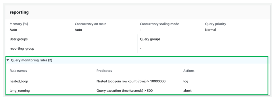
For the reporting queue, add the following QMRs:

  • nested_loop – Logs any query involved in a nested loop join that results in a row count more than 10,000,000 rows.
  • long_running – Stops queries that run for more than 300 seconds (5 minutes).

For the adhoc queue, add the following QMRs:

  • returned_rows – Stops any query that returns more than 1,000,000 rows back to the calling client application (this isn’t practical and can degrade the end-to-end performance of the application).
  • spectrum_scan – Stops any query that scans more than 1000 MB of data from an Amazon Simple Storage Service (Amazon S3) data lake by using Redshift Spectrum.

Attach the custom parameter group to the cluster

To attach the custom parameter group to your provisioned Redshift cluster, follow the instructions in Associating a parameter group with a cluster. If you don’t already have a provisioned Redshift cluster, refer to Create a cluster.

For this post, we attached our custom parameter group csblog to an already created provisioned Amazon Redshift cluster.

Create an SNS topic

In this step, you create an SNS topic that receives a detailed message of QMR violation from the Lambda function that checks the Amazon Redshift system table for QMR violation entries. For instructions, refer to Creating an Amazon SNS topic.

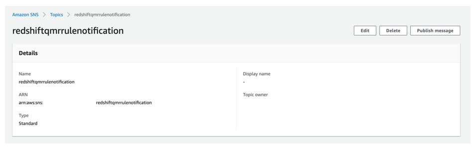
For this post, we created an SNS topic named redshiftqmrrulenotification.

Create a Lambda function to monitor the system table

In this step, you create a Lambda function that monitors the STL_WLM_RULE_ACTION system table. Whenever any record is found in the table since the last time the function ran, the function publishes a detailed message to the SNS topic that you created earlier. You also create an EventBridge rule to invoke the function every 5 minutes.

For this post, we create a Lambda function named redshiftqmrrule that is scheduled to run every 5 minutes via an EventBridge rule named Redshift-qmr-rule-Lambda-schedule. For instructions, refer to Building Lambda functions with Python.

The following screenshot shows the function that checks the pg_catalog.stl_wlm_rule_action table.

To create an EventBridge rule and associate it with the Lambda function, refer to Create a Rule.

The following screenshot shows the EventBridge rule Redshift-qmr-rule-Lambda-schedule, which calls the function every 5 minutes.

We use the following Python 3.9 code for this Lambda function. The function uses an Amazon Redshift Data API call that uses GetClusterCredentials for temporary credentials.

import json
import time
import unicodedata
import traceback
import sys
from pip._internal import main
import urllib3
import os
import boto3
from datetime import datetime

# initiate redshift-data client in boto3
client = boto3.client("redshift-data")

query = "select userid,query,service_class,trim(rule) as rule,trim(action) as action,recordtime from stl_wlm_rule_action WHERE userid > 1 AND recordtime >= current_timestamp AT TIME ZONE 'UTC' - INTERVAL '5 minute' order by recordtime desc;"
sns = boto3.resource('sns')
sns_arn = os.environ['sns_arn']
platform_endpoint = sns.PlatformEndpoint('{sns_arn}'.format(sns_arn = sns_arn))

def status_check(client, query_id):
    desc = client.describe_statement(Id=query_id)
    status = desc["Status"]
    if status == "FAILED":
        raise Exception('SQL query failed:' + query_id + ": " + desc["Error"])
    return status.strip('"')

def execute_sql(sql_text, redshift_database, redshift_user, redshift_cluster_id):
    print("Executing: {}".format(sql_text))
    res = client.execute_statement(Database=redshift_database, DbUser=redshift_user, Sql=sql_text,
                                   ClusterIdentifier=redshift_cluster_id)
    
    query_id = res["Id"]
    print("query id")
    print(query_id)
    done = False
    while not done:
        time.sleep(1)
        status = status_check(client, query_id)
        if status in ("FAILED", "FINISHED"):
            print("status is: {}".format(status))
            break
    return query_id

def publish_to_sns(message):
    try:
        # Publish a message.
        response = platform_endpoint.publish(
                  Subject='Redshift Query Monitoring Rule Notifications',
                  Message=message,
                  MessageStructure='string'

            )
        return  response

    except:
        print(' Failed to publish messages to SNS topic: exception %s' % sys.exc_info()[1])
        return 'Failed'

def lambda_handler(event, context):
    
    rsdb = os.environ['rsdb']
    rsuser = os.environ['rsuser']
    rscluster = os.environ['rscluster']
    #print(query)
    res = execute_sql(query, rsdb, rsuser, rscluster)
    print("res")
    print(res)
    response = client.get_statement_result(
        Id = res
    )
    # datetime object containing current date and time
    now = datetime.now()
    dt_string = now.strftime("%d-%b-%Y %H:%M:%S")
    print(response) 
    if response['TotalNumRows'] > 0:
        messageText = '################## Reporting Begin' + ' [' + str(dt_string) + ' UTC] ##################\n\n'
        messageText = messageText + 'Total number of queries affected by QMR Rule violation for Redshift cluster "' + rscluster + '" is ' + str(len(response['Records'])) + '.' + '\n' + '\n'
        for i in range(len(response['Records'])):
            messageText = messageText + 'It was reported at ' + str(response['Records'][i][5]['stringValue'])[11:19] + ' UTC on ' + str(response['Records'][i][5]['stringValue'])[0:10] + ' that a query with Query ID - ' + str(response['Records'][i][1]['longValue']) + ' had to ' +  str(response['Records'][i][4]['stringValue']) + ' due to violation of QMR Rule "' + str(response['Records'][i][3]['stringValue']) + '".\n'
        messageText = messageText + '\n########################### Reporting End ############################\n\n'
        query_result_json = messageText
        response = publish_to_sns(query_result_json)
    else:
        print('No rows to publish to SNS')

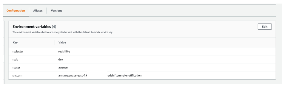
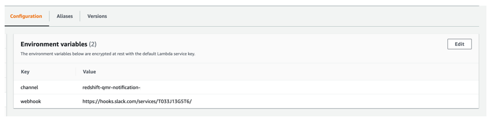
We use four environment variables for this Lambda function:

  • rscluster – The Amazon Redshift provisioned cluster identifier
  • rsdb – The Amazon Redshift database where you’re running these tests
  • rsuser – The Amazon Redshift user who has the privilege to run queries on pg_catalog.stl_wlm_rule_action
  • sns_arn – The Amazon Resource Name (ARN) of the SNS topic that we created earlier

Create Slack resources

In this step, you create a new Slack workspace (if you don’t have one already), a new private Slack channel (only if you don’t have one or don’t want to use an existing one), and a new Slack app in the Slack workspace. For instructions, refer to Create a Slack workspace, Create a channel, and Creating an app.

For this post, we created the following resources in the Slack website and Slack desktop app:

  • A Slack workspace named RedshiftQMR*****
  • A private channel, named redshift-qmr-notification-*****-*******, in the newly created Slack workspace
  • A new Slack app in the Slack workspace, named RedshiftQMRRuleNotification (using the From Scratch option)

Add an incoming webhook and authorize Slack app

In this step, you enable and add an incoming webhook to the Slack workspace that you created. For full instructions, refer to Enable Incoming Webhooks and Create an Incoming Webhook. You also authorize your Slack app so that it can post messages to the private Slack channel.

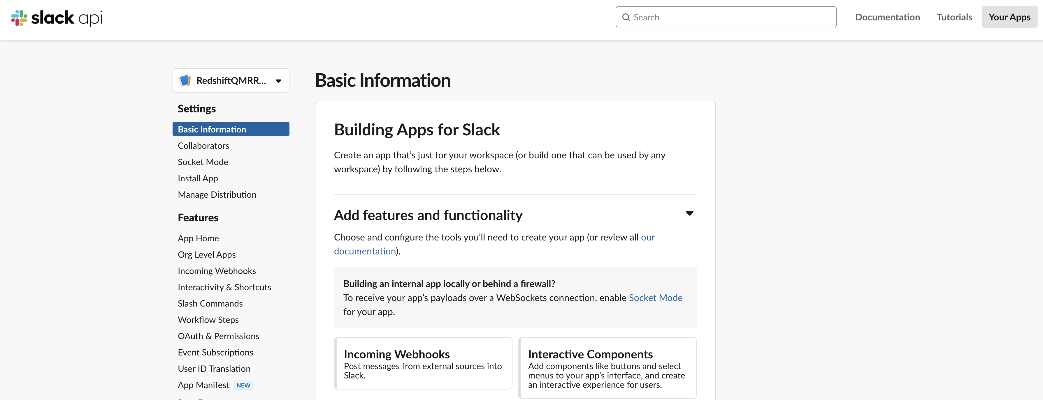
  1. In the Slack app, under Settings in the navigation pane, choose Basic Information.
  2. Choose Incoming Webhooks.
  3. Turn on Activate Incoming Webhooks.
  4. Choose Add New Webhook to Workspace.
  5. Authorize the Slack app RedshiftQMRRuleNotification so that it can post messages to the private Slack channel redshift-qmr-notification-*****-*******.

The following screenshot shows the details of the newly added incoming webhook.

Create a second Lambda function and subscribe to the SNS topic

In this step, you create a second Lambda function that is subscribed to the SNS topic that you created earlier. For full instructions, refer to Building Lambda functions with Python and Subscribing a function to a topic.

For this post, we create a second function named redshiftqmrrulesnsinvoke, which is subscribed to the SNS topic redshiftqmrrulenotification. The second function sends a detailed QMR violation message (received from the SNS topic) to the designated Slack channel named redshift-qmr-notification-*. This function uses the incoming Slack webhook that we created earlier.

We also create an SNS subscription of the second Lambda function to the SNS topic that we created previously.

The following is the Python 3.9 code used for the second Lambda function:

import urllib3
import json
import os

http = urllib3.PoolManager()
def lambda_handler(event, context):
    
    url = os.environ['webhook']
    channel = os.environ['channel']
    msg = {
        "channel": channel,
        "username": "WEBHOOK_USERNAME",
        "text": event['Records'][0]['Sns']['Message'],
        "icon_emoji": ""
    }
    
    encoded_msg = json.dumps(msg).encode('utf-8')
    resp = http.request('POST',url, body=encoded_msg)
    print({
        "message": event['Records'][0]['Sns']['Message'], 
        "status_code": resp.status, 
        "response": resp.data
    })

We use two environment variables for the second Lambda function:

  • channel – The Slack channel that we created
  • webhook – The Slack webhook that we created

Test the solution

To show the effect of the QMRs, we ran queries that violate the QMRs we set up.

Test 1: Returned rows

Test 1 looks for violations of the returned_rows QMR, in which the return row count is over 1,000,000 for a query that ran in the adhoc queue.

We created and loaded a table named lineitem in a schema named aquademo, which has more than 18 billion records. You can refer to the GitHub repo to create and load the table.

We ran the following query, which violated the returned_rows QMR, and the query was stopped as specified in the action set in the QMR.

select * from aquademo.lineitem limit 1000001;

The following screenshot shows the view from the Amazon Redshift client after running the query.

The following screenshot shows the view on the Amazon Redshift console.

The following screenshot shows the notification we received in our Slack channel.

Test 2: Long-running queries

Test 2 looks for violations of the long_running QMR, in which query runtime is over 300 seconds for a user who belongs to reporting_group.

In the following code, we created a new Amazon Redshift group named reporting_group and added a new user, named reporting_user, to the group. reporting_group is assigned USAGE and SELECT privileges on all tables in the retail and aquademo schemas.

create group reporting_group;
create user reporting_user in group reporting_group password 'Test12345';
grant usage on schema retail,aquademo to group reporting_group;
grant select on all tables in schema retail,aquademo to group reporting_group;

We set the session authorization to reporting_user so the query runs in the reporting queue. We ran the following query, which violated the long_running QMR, and the query was stopped as specified in the action set in the QMR:

set session authorization reporting_user;
set enable_result_cache_for_session  to off;
select * from aquademo.lineitem;

The following screenshot shows the view from the Amazon Redshift client.

The following screenshot shows the view on the Amazon Redshift console.

The following screenshot shows the notification we received in our Slack channel.

Test 3: Nested loops

Test 3 looks for violations of the nested_loop QMR, in which the nested loop join row count is over 10,000,000 for a user who belongs to reporting_group.

We set the session authorization to reporting_user so the query runs in the reporting queue. We ran the following query, which violated the nested_loop QMR, and the query logged the violation as specified in the action set in the QMR:

set session authorization reporting_user;
set enable_result_cache_for_session  to off;
select ss.*,cd.* 
from retail.store_sales ss
, retail.customer_demographics cd;

Before we ran the original query, we also checked the explain plan and noted that this nested loop will return more than 10,000,000 rows. The following screenshot shows the query explain plan.

The following screenshot shows the notification we received in our Slack channel.

Test 4: Redshift Spectrum scans

Test 4 looks for violations of the spectrum_scan QMR, in which Redshift Spectrum scans exceed 1000 MB for a query that ran in the adhoc queue.

For this example, we used store_sales data (unloaded from an Amazon Redshift table that was created by using the TPC-DS benchmark data) loaded in an Amazon S3 location. Data in Amazon S3 is non-partitioned under one prefix and has a volume around 3.9 GB. We created an external schema (qmr_spectrum_rule_test) and external table (qmr_rule_store_sales) in Redshift Spectrum.

We used the following steps to run this test with the sample data:

  1. Run an unload SQL command:
    unload ('select * from store_sales')
    to 's3://<<Your Amazon S3 Location>>/store_sales/' 
    iam_role default;

  2. Create an external schema from Redshift Spectrum:
    CREATE EXTERNAL SCHEMA if not exists qmr_spectrum_rule_test
    FROM DATA CATALOG DATABASE 'qmr_spectrum_rule_test' region 'us-east-1' 
    IAM_ROLE default
    CREATE EXTERNAL DATABASE IF NOT exists;

  3. Create an external table in Redshift Spectrum:
    create external table qmr_spectrum_rule_test.qmr_rule_store_sales
    (
    ss_sold_date_sk int4 ,            
      ss_sold_time_sk int4 ,     
      ss_item_sk int4  ,      
      ss_customer_sk int4 ,           
      ss_cdemo_sk int4 ,              
      ss_hdemo_sk int4 ,         
      ss_addr_sk int4 ,               
      ss_store_sk int4 ,           
      ss_promo_sk int4 ,           
      ss_ticket_number int8 ,        
      ss_quantity int4 ,           
      ss_wholesale_cost numeric(7,2) ,          
      ss_list_price numeric(7,2) ,              
      ss_sales_price numeric(7,2) ,
      ss_ext_discount_amt numeric(7,2) ,             
      ss_ext_sales_price numeric(7,2) ,              
      ss_ext_wholesale_cost numeric(7,2) ,           
      ss_ext_list_price numeric(7,2) ,               
      ss_ext_tax numeric(7,2) ,                 
      ss_coupon_amt numeric(7,2) , 
      ss_net_paid numeric(7,2) ,   
      ss_net_paid_inc_tax numeric(7,2) ,             
      ss_net_profit numeric(7,2)                     
    ) ROW FORMAT DELIMITED 
      FIELDS TERMINATED BY '|' 
    STORED AS INPUTFORMAT 
      'org.apache.hadoop.mapred.TextInputFormat' 
    OUTPUTFORMAT 
      'org.apache.hadoop.hive.ql.io.HiveIgnoreKeyTextOutputFormat'
    LOCATION
      's3://<<Your Amazon S3 Location>>/store_sales/'
    TABLE PROPERTIES (
      'averageRecordSize'='130', 
      'classification'='csv', 
      'columnsOrdered'='true', 
      'compressionType'='none', 
      'delimiter'='|', 
      'recordCount'='11083990573', 
      'sizeKey'='1650877678933', 
      'typeOfData'='file');

  4. Run the following query:
    select * 
    FROM qmr_spectrum_rule_test.qmr_rule_store_sales 
    where ss_sold_date_sk = 2451074;

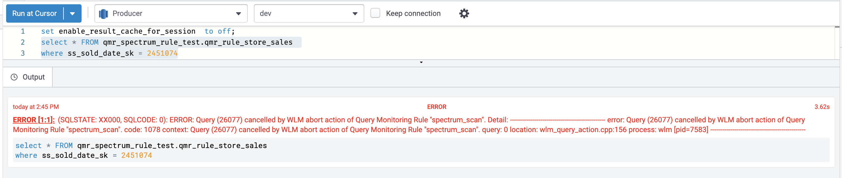
The query violated the spectrum_scan QMR, and the query was stopped as specified in the action set in the QMR.

The following screenshot shows the view from the Amazon Redshift client.

The following screenshot shows the view on the Amazon Redshift console.

The following screenshot shows the notification we received in our Slack channel.

Clean up

When you’re finished with this solution, we recommend deleting the resources you created to avoid incurring any further charges.

Conclusion

Amazon Redshift is a powerful, fully managed data warehouse that can offer significantly increased performance and lower cost in the cloud. In this post, we discussed how you can automate notification of misbehaving queries on Slack by using query monitoring rules. QMRs can help you maximize cluster performance and throughput when supporting mixed workloads. Use these instructions to set up your Slack channel to receive automatic notifications from your Amazon Redshift cluster for any violation of QMRs.


About the Authors

Dipankar Kushari is a Senior Specialist Solutions Architect in the Analytics team at AWS.

Harshida Patel is a Specialist Senior Solutions Architect in the Analytics team at AWS.
Share data securely across Regions using Amazon Redshift data sharing

Post Syndicated from Rahul Chaturvedi original https://aws.amazon.com/blogs/big-data/share-data-securely-across-regions-using-amazon-redshift-data-sharing/

Today’s global, data-driven organizations treat data as an asset and use it across different lines of business (LOBs) to drive timely insights and better business decisions. This requires you to seamlessly share and consume live, consistent data as a single source of truth without copying the data, regardless of where LOB users are located.

Amazon Redshift is a fast, scalable, secure, and fully managed data warehouse that enables you to analyze all your data using standard SQL easily and cost-effectively. Amazon Redshift data sharing allows you to securely share live, transactionally consistent data in one Amazon Redshift cluster with another Amazon Redshift cluster across accounts and Regions, without needing to copy or move data from one cluster to the other.
Amazon Redshift data sharing was initially launched in March 2021, and support for cross-account data sharing was added in August 2021. Cross-Region support became generally available in February 2022. This provides full flexibility and agility to easily share data across Amazon Redshift clusters in the same AWS account, different accounts, or different Regions.

In this post, we discuss how to configure cross-Region data sharing between different accounts or in the same account.

Solution overview

It’s easy to set up cross-account and cross-Region data sharing from producer to consumer clusters, as shown in the following flow diagram. The workflow consists of the following components:

  • Producer cluster administrator – The producer admin is responsible for the following:
    • Create an Amazon Redshift database share (a new named object to serve as a unit of sharing, referred to as a datashare) on the AWS Management Console
    • Add database objects (schemas, tables, views) to the datashare
    • Specify a list of consumers that the objects should be shared with
  • Consumer cluster administrator – The consumer admin is responsible for the following:
    • Examine the datashares that are made available and review the content of each share
    • Create an Amazon Redshift database from the datashare object
    • Assign permissions on this database to appropriate users and group in the consumer cluster
  • Users and groups in the consumer cluster – Users and groups can perform the following actions:
    • List the shared objects as part of standard metadata queries
    • Start querying immediately

In the following sections, we discuss use cases and how to implement the cross-Region sharing feature between different accounts or in the same account.

Use cases

Common use cases for the data sharing feature include implementing multi-tenant patterns, data sharing for workload isolation, and security considerations related to data sharing.

In this post, we demonstrate cross-Region data sharing, which is especially useful for the following use cases:

  • Support for different kinds of business-critical workloads – You can use a central extract, transform, and load (ETL) cluster that shares data with multiple business intelligence (BI) or analytic clusters owned by geographically distributed business groups
  • Enabling cross-group collaboration – The solution enables seamless collaboration across teams and business groups for broader analytics, data science, and cross-product impact analysis
  • Delivering data as a service – You can share data as a service across your organization
  • Sharing data between environments – You can share data among development, test, and production environments at different levels of granularity
  • Licensing access to data in Amazon Redshift – You can publish Amazon Redshift datasets in the AWS Data Exchange that customers can find, subscribe to, and query in minutes.

Cross-Region data sharing between different accounts

In this use case, we share data from a cluster in an account in us-east-1 with a cluster owned by a different account in us-west-2. The following diagram illustrates this architecture.

When setting up cross-Region data sharing across different AWS accounts, there’s an additional step to authorize a datashare on the producer account and associate the datashare on the consumer account. The reason is that for such shares that go outside of your account or organization, you must have a two-step authentication process. For example, consider a scenario where the database analyst creates a database share using the console and now requires the producer administrator to authorize this datashare. For same-account sharing, we don’t require that two-step approach because you’re granting access within the perimeter of your own account.

This setup broadly follows a four-step process:

  1. Create a datashare on the producer account.
  2. Authorize the datashare on the producer account.
  3. Associate the datashare on the consumer account.
  4. Query the datashare.

Create a datashare

To create your datashare, complete the following steps:

  1. On the Amazon Redshift console, create a producer cluster with encryption enabled.

This is in your source account. For instructions on how to automate process of creating an Amazon Redshift cluster, refer to Automate building an integrated analytics solution with AWS Analytics Automation Toolkit.

On the Datashares tab, no datashares are currently available on the producer account.

  1. Create a consumer cluster with encryption enabled in a different AWS account and different Region.

This is your target account. On the Datashares tab, no datashares are currently available on the consumer side.

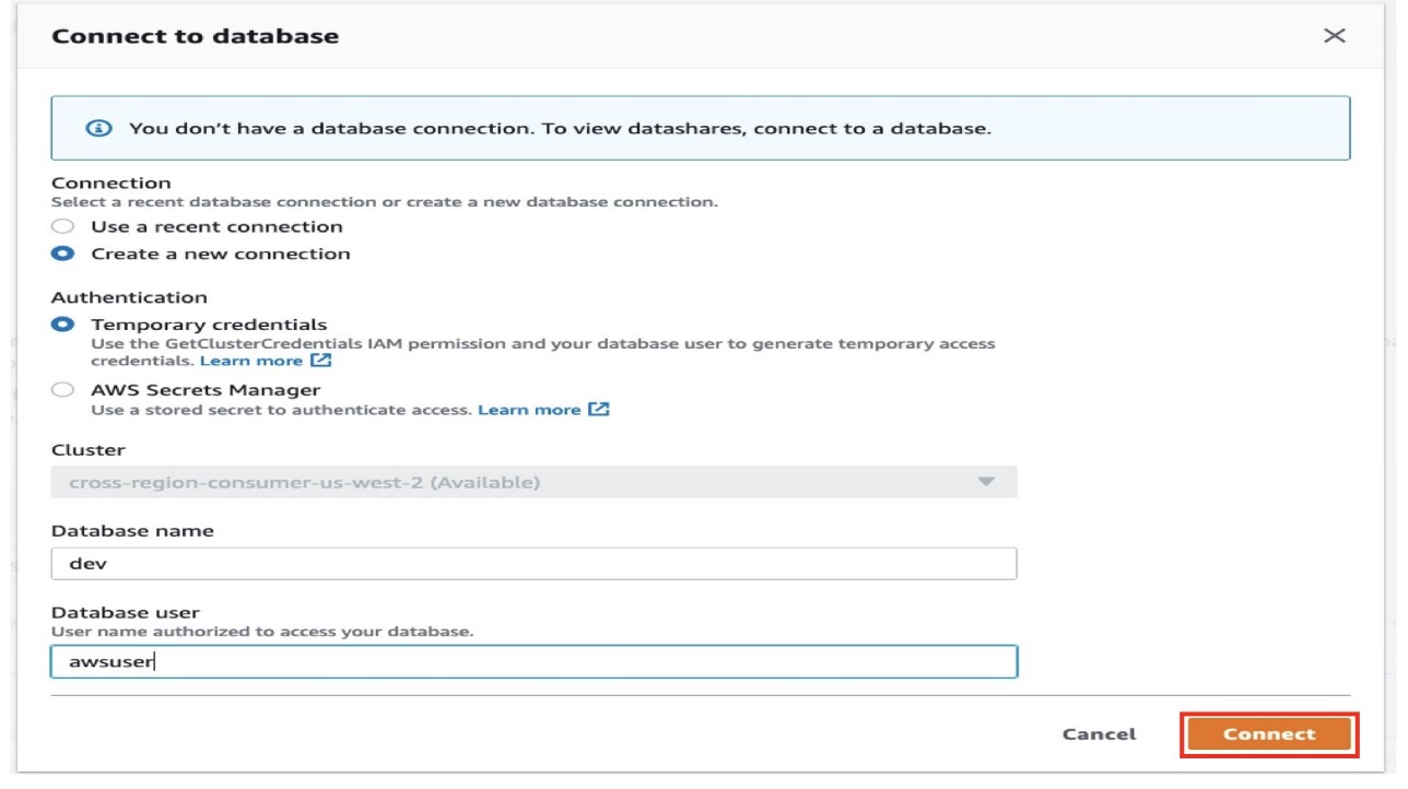
  1. Choose Connect to database to start setting up your datashare.
  2. For Connection, select Create a new connection.

You can connect to the database using either temporary credentials or AWS Secrets Manager. Refer to Querying a database using the query editor to learn more about these two connection options. We use temporary credentials in this post.

  1. For Authentication, select Temporary credentials.
  2. For Database name, enter a name (for this post, dev).
  3. For Database user, enter the user authorized to access the database (for this post, awsuser).
  4. Choose Connect.
  5. Repeat these steps on the producer cluster.
  6. Next, create a datashare on the producer.
  7. For Datashare type, select Datashare.
  8. For Database name, enter a name.
  9. For Database name, choose the database you specified earlier.
  10. For Publicly accessible, select Enable.
  11. In the Datashare objects section, choose Add to add the database schemas and tables to share.\

In our case, we add all tables and views from the public schema to the datashare.

  1. Choose Add.

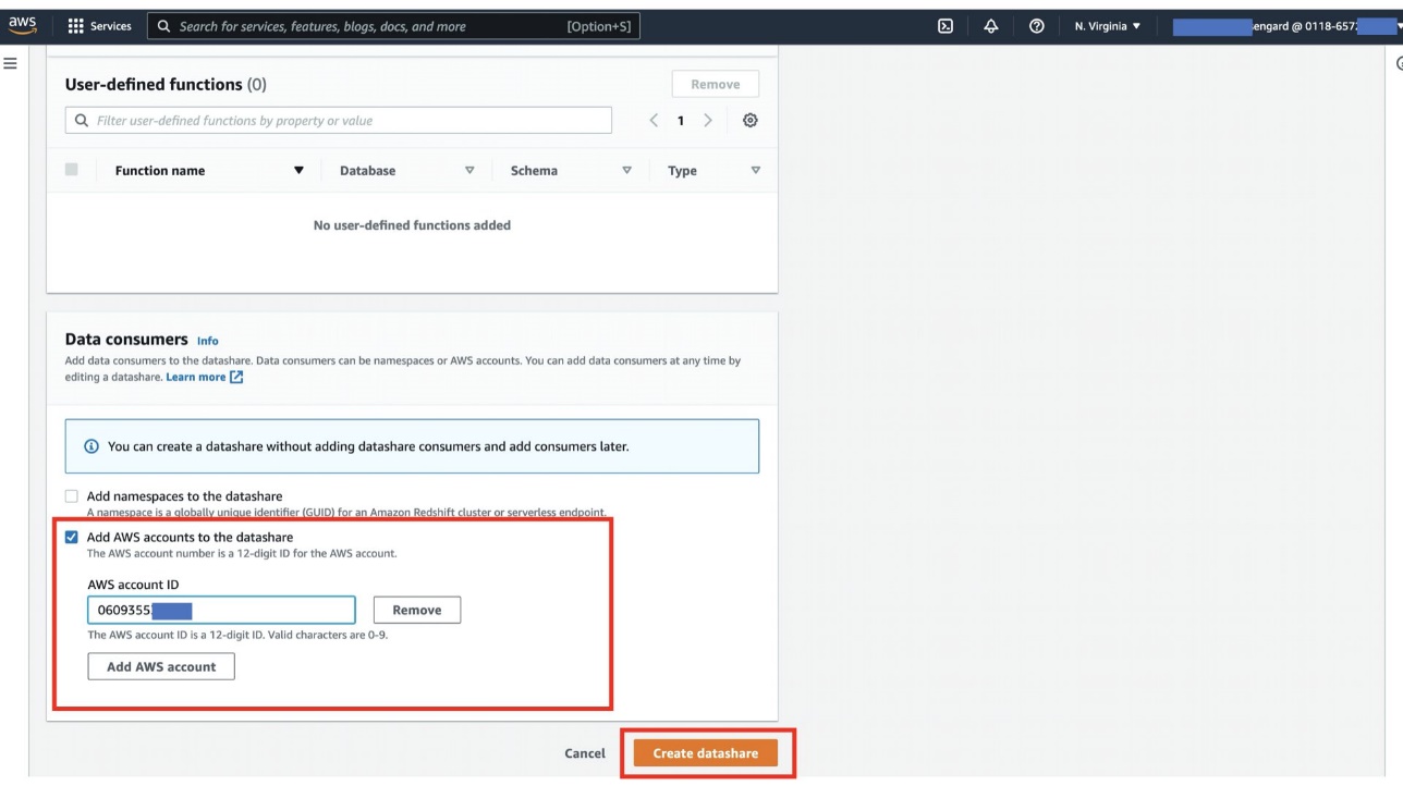
Next, you add the consumer account in order to add a cross-account, cross-Region consumer to this datashare.

  1. In the Data consumers section, select Add AWS accounts to the datashare and enter your AWS account ID.
  2. Choose Create datashare.

Authorize the datashare

To authorize this datashare, complete the following steps:

  1. On the Amazon Redshift console, choose Datashares in the navigation pane.
  2. Choose the datashare you created earlier.
  3. In the Data consumers section, select the data consumer ID and choose Authorize.
  4. Choose Authorize to confirm.

Associate the datashare

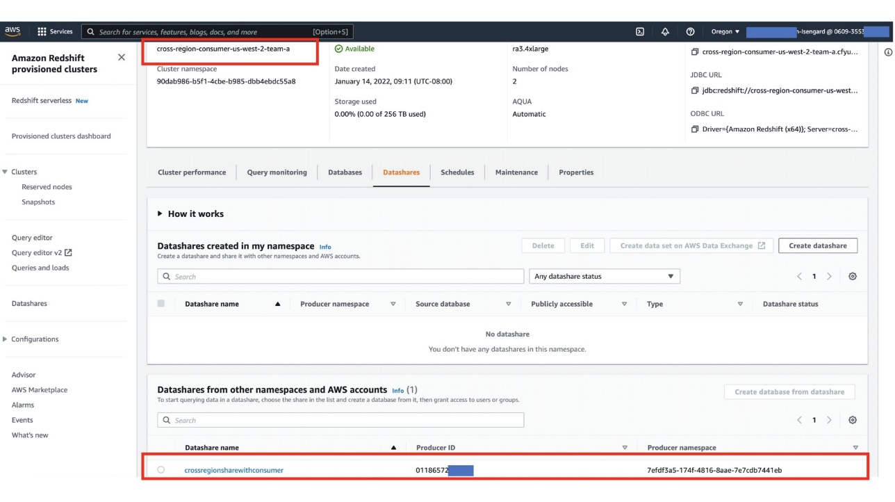
On the consumer account in a different Region, we have multiple clusters. In this step, the consumer administrator associates this datashare to only to one of those clusters. As a consumer, you have the option to accept or decline a datashare. We associate this datashare to cross-region-us-west-2-team-a.

  1. On the Datashares page, choose the From other accounts tab to find the database you created in the source account.
  2. Select the appropriate datashare and choose Associate.

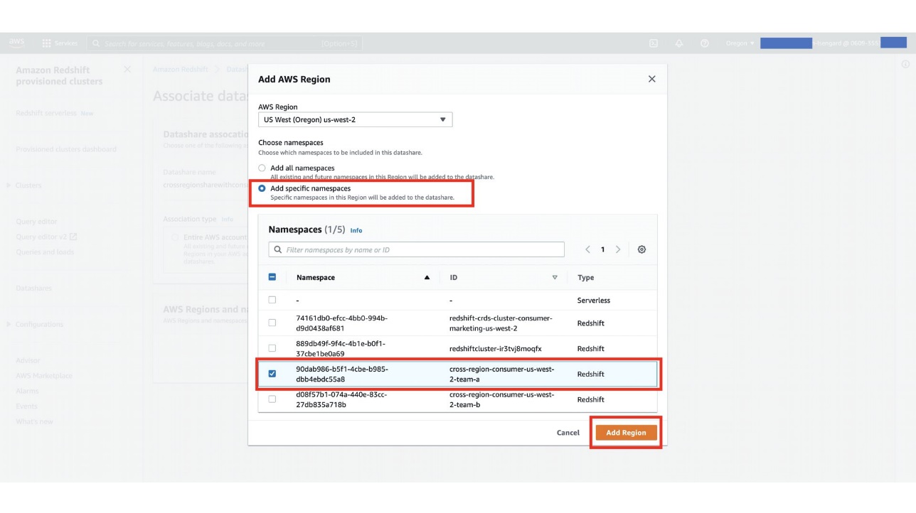
In the next step, you as a consumer admin have the option to associate the datashare with specific clusters in a different Region. Each cluster has its own globally unique identifier, known as a namespace. For this post, we associate the datashare to cluster cross-region-us-west-2-team-a with the namespace 90dab986-b5f1-4cbe-b985-dbb4ebdc55a8 in the us-west-2 Region.

  1. For Choose namespaces, select Add specific namespaces.
  2. Select your namespace and choose Add Region.
  3. Choose Clusters in the navigation pane.
  4. Choose the cluster that you authorized access to the datashare.
  5. On the Datashares tab, confirm the datashare from the producer cluster is listed in the Datashares from other namespaces and AWS accounts section.

Query the datashare

You can query shared data using standard SQL interfaces, JDBC or ODBC drivers, and the Data API. You can also query data with high performance from familiar BI and analytic tools. You can run queries by referring to the objects from other Amazon Redshift databases that are both local to and remote from your cluster that you have permission to access.

You can do so simply by staying connected to local databases in your cluster. Then you can create consumer databases from datashares to consume shared data.

After you have done so, you can run cross-database queries joining the datasets. You can query objects in consumer databases using the three-part notation consumer_database_name.schema_name.table_name. You can also query using external schema links to schemas in the consumer database. You can query both local data and data shared from other clusters within the same query. Such a query can reference objects from the current connected database and from other non-connected databases, including consumer databases created from datashares.

  1. On the consumer cluster, create a database to map the datashare objects to your cluster.
  2. You can now join your local schema objects with the objects in the shared database in a single query.

You can access the shared objects using a three-part notation, as highlighted in the following query:

select a.c_custkey,count(b.o_orderkey) as cnt_of_orders
from dev.public.customer a
join producerdata.public.orders b
on a.c_custkey = b.o_custkey
group by 1
order by cnt_of_orders desc 
limit 5;

The following screenshot shows our query results.

One alternative to using three-part notation is to create external schemas for the shared objects. As shown in the following code, we create producerSchema to map the datashare schema to a local schema:

Create external schema producerSchema
From REDSHIFT DATABASE ‘producerdata’ schema ‘public’;

Cross-Region data sharing in the same account

When setting up cross-Region data sharing in the same account, we don’t need to follow the authorize-associate flow on the console. We can easily configure this share using SQL commands. Complete the following steps:

  1. On the consumer cluster, run the following SQL statement to get the current namespace:
    select current_namespace;

The following screenshot shows our results.

  1. On the producer cluster, run the SQL commands as shown in the following screenshot.

This step involves creating a datashare and making it publicly accessible so that the consumer can access it from across the Region. It then adds the database objects to the datashare, followed by granting permissions on this datashare to the consumer namespace. Use your consumer namespace from the previous step.

  1. Capture the producer namespace from the producer cluster to use in the next step.

The consumer cluster now has access to the datashare that was created on the producer.

  1. You can verify this from svv_datashares.
  2. After you confirm that the datashare is available on consumer, the next step is to map the objects of the datashare to a database in order to start querying them, as shown in the following screenshots.

Considerations for using cross-Region data sharing

Keep in mind the following when using cross-Region data sharing:

  • You must enable encryption both the producer and consumer accounts.
  • For cross-Region data sharing, the consumer pays the cross-Region data transfer fee from the producer Region to the consumer Region based on the price of Amazon Simple Storage Service (Amazon S3), in addition to the cost of using the Amazon Redshift cluster.
  • You can’t share stored procedures and Python UDF functions.
  • This feature is only supported on the RA3 instance type.
  • The producer cluster administrator is responsible for implementing any Region locality and compliance requirements (such as GDPR) by performing the following actions:
    • Share only data that can be shared outside a Region in a datashare.
    • Authorize the appropriate data consumer to access the datashare.
  • The performance of the queries on data shared across Regions depends on the compute capacity of the consumer clusters.
  • Network throughput between different Regions could yield different query performance. For instance, data sharing from us-east-1 to us-east-2 could yield better performance compared to us-east-1 to ap-northeast-1.

Summary

Amazon Redshift cross-Region data sharing is now available. Previously, data sharing was only allowed within the same Region. With this launch, you can share data across Regions with clusters residing in the same account or different accounts.

We look forward to hearing from you about your experience. If you have questions or suggestions, please leave a comment.


About the Authors

Rahul Chaturvedi is an Analytics Specialist Solutions Architect AWS. Prior to this role, he was a Data Engineer at Amazon Advertising and Prime Video, where he helped build petabyte-scale data lakes for self-serve analytics.

Kishore Arora is a Sr Analytics Specialist Solutions Architect at AWS. In this role, he helps customers modernize their data platform and architect big data solutions with AWS purpose-built data services. Prior to this role, he was a big data architect and delivery lead working with Tier-1 telecom customers.

BP Yau is a Sr Product Manager at AWS. He is passionate about helping customers architect big data solutions to process data at scale. Before AWS, he helped Amazon.com Supply Chain Optimization Technologies migrate its Oracle data warehouse to Amazon Redshift and build its next generation big data analytics platform using AWS technologies.

Srikanth Sopirala is a Principal Analytics Specialist Solutions Architect at AWS. He is a seasoned leader with over 20 years of experience, who is passionate about helping customers build scalable data and analytics solutions to gain timely insights and make critical business decisions. In his spare time, he enjoys reading, spending time with his family, and road cycling.

Sharing security expertise through CodeQL packs (Part I)

Post Syndicated from Andrew Eisenberg original https://github.blog/2022-04-19-sharing-security-expertise-through-codeql-packs-part-i/

Congratulations! You’ve discovered a security bug in your own code before anyone has exploited it. It’s a big relief. You’ve created a CodeQL query to find other places where this happens and ensure this will never happen again, and you’ve deployed your new query to be run on every pull request in your repo to prevent similar mistakes from ever being made again.

What’s the best way to share this knowledge with the community to help protect the open source ecosystem by making sure that the same vulnerability is never introduced into anyone’s codebase, ever?

The short answer: produce a CodeQL pack containing your queries, and publish them to GitHub. CodeQL packaging is a beta feature in the CodeQL ecosystem. With CodeQL packaging, your expertise is documented, concise, executable, and easily shareable.

This is the first post of a two-part series on CodeQL packaging. In this post, we show how to use CodeQL packs to share security expertise. In the next post, we will discuss some of our implementation and design decisions.

Modeling a vulnerability in CodeQL

CodeQL’s customizability makes it great for detecting vulnerabilities in your code. Let’s use the Exec call vulnerable to binary planting query as an example. This query was developed by our team in response to discovering a real vulnerability in one of our open source repositories.

The purpose of this query is to detect executables that are potentially vulnerable to Windows binary planting, an exploit where an attacker could inject a malicious executable into a pull request. This query is meant to be evaluated on JavaScript code that is run inside of a GitHub Action. It matches all arguments to calls to the ToolRunner (a GitHub Action API) where the argument has not been sanitized (that is, ensured to be safe) by having been wrapped in a call to safeWhich. The implementation details of this query are not relevant to this post, but you can explore this query and other domain-specific queries like it in the repository.

This query is currently protecting us on every pull request, but in its current form, it is not easily available for others to use. Even though this vulnerability is relatively difficult to attack, the surface area is large, and it could affect any GitHub Action running on Windows in public repositories that accept pull requests. You could write a stern blog post on the dangers of invoking unqualified Windows executables in untrusted pull requests (maybe you’re even reading such a post right now!), but your impact will be much higher if you could share the query to help anyone find the bug in their code. This is where CodeQL packaging comes in. Using CodeQL packaging, not only can developers easily learn about the binary planting pattern, but they can also automatically apply the pattern to find the bug in their own code.

Sharing queries through CodeQL packs

If you think that your query is general purpose and applicable to all repositories in all situations, then it is best to contribute it to our open source CodeQL query repository (and collect a bounty in the process!). That way, your query will be run on every pull request on every repository that has GitHub code scanning enabled.

However, many (if not most) queries are domain specific and not applicable to all repositories. For example, this particular binary planting query is only applicable to GitHub Actions implemented in JavaScript. The best way to share such queries query is by creating a CodeQL pack and publishing it to the CodeQL package registry to make it available to the world. Once published, CodeQL packs are easily shared with others and executed in their CI/CD pipeline.

There are two kinds of CodeQL packs:

  • Query packs, which contain a set of pre-compiled queries that can be easily evaluated on a CodeQL database.
  • Library packs, which contain CodeQL libraries (*.qll files), but do not contain any runnable queries. Library packs are meant to be used as building blocks to produce other query packs or library packs.

In the rest of this post, we will show you how to create, share, and consume a CodeQL query pack. Library packs will be introduced in a future blog post.

To create a CodeQL pack, you’ll need to make sure that you’ve installed and set up the CodeQL CLI. You can follow the instructions here.

The next step is to create a qlpack.yml file. This file declares the CodeQL pack and information about it. Any *.ql files in the same directory (or sub-directory) as a qlpack.yml file are considered part of the package. In this case, you can place binary-planting.ql next to the qlpack.yml file.

Here is the qlpack.yml from our example:

name: aeisenberg/codeql-actions-queries
version: 1.0.1
dependencies:
 codeql/javascript-all: ~0.0.10

All CodeQL packs must have a name property. If they are going to be published to the CodeQL registry, then they must have a scope as part of the name. The scope is the part of the package name before the slash (in this example: aeisenberg). It should be the username or organization on github.com that will own this package. Anyone publishing a package must have the proper privileges to do so for that scope. The name part of the package name must be unique within the scope. Additionally, a version, following standard semver rules, is required for publishing.

The dependencies block lists all of the dependencies of this package and their compatible version ranges. Each dependency is referenced as the scope/name of a CodeQL library pack, and each library pack may in turn depend on other library packs declared in their qlpack.yml files. Each query pack must (transitively) depend on exactly one of the core language packs (for example, JavaScript, C#, Ruby, etc.), which determines the language your query can analyze.

In this query pack, the standard JavaScript libraries, codeql/javascript-all, is the only dependency and the semver range ~0.0.10 means any version >= 0.0.10 and < 0.1.0 suffices.

With the qlpack.yml defined, you can now install all of your declared dependencies. Run the codeql pack install command in the root directory of the CodeQL pack:

$ codeql pack install
Dependencies resolved. Installing packages...
Install location: /Users/andrew.eisenberg/.codeql/packages
Installed fresh codeql/[email protected]

After making any changes to the query, you can then publish the query to the GitHub registry. You do this by running the codeql pack publish command in the root of the CodeQL pack.

Here is the output of the command:

$ codeql pack publish
Running on packs: aeisenberg/codeql-actions-queries.
Bundling and then publishing qlpack located at '/Users/andrew.eisenberg/git-repos/codeql-actions-queries'.
Bundled qlpack created at '/var/folders/41/kxmfbgxj40dd2l_x63x9fw7c0000gn/T/codeql-docker17755193287422157173/.Docker Package Manager/codeql-actions-queries.1.0.1.tgz'.
Packaging> Package 'aeisenberg/codeql-actions-queries' will be published to registry 'https://ghcr.io/v2/' as 'aeisenberg/codeql-actions-queries'.
Packaging> Package 'aeisenberg/[email protected]' will be published locally to /Users/andrew.eisenberg/.codeql/packages/aeisenberg/codeql-actions-queries/1.0.1
Publish successful.

You have successfully published your first CodeQL pack! It is now available in the registry on GitHub.com for anyone else to run using the CodeQL CLI. You can view your newly-published package on github.com:

CodeQL pack on github.com

At the time of this writing, packages are initially uploaded as private packages. If you want to make it public, you must explicitly change the permissions. To do this, go to the package page, click on package settings, then scroll down to the Danger Zone:

Danger Zone!

And click Change visibility.

Running queries from CodeQL packs using the CodeQL CLI

Running the queries in a CodeQL pack is simple using the CodeQL CLI. If you already have a database created, just call the codeql database analyze command with the --download option, passing a reference to the package you want to use in your analysis:

$ codeql database analyze --format=sarif-latest --output=out.sarif --download my-db aeisenberg/codeql-actions-queries@^1.0.1

The --download option asks CodeQL to download any CodeQL packs that aren’t already available. The ^1.0,0 is optional and specifies that you want to run the latest version of the package that is compatible with ^1.0.1. If no version range is specified, then the latest version is always used. You can also pass a list of packages to evaluate. The CodeQL CLI will download and cache each specified package and then run all queries in their default query suite.

To run a subset of queries in a pack, add a : and a path after it:

aeisenberg/codeql-actions-queries@^1.0.1:binary-planting.ql

Everything after the : is interpreted as a path relative to the root of the pack, and you can specify a single query, a query directory, or a query suite (.qls file).

Evaluating CodeQL packs from code scanning

Run the queries from your CodeQL pack in GitHub code scanning is easy! In your code scanning workflow, in the github/codeql-action/init step, add packs entry to list the packs you want to run:

- uses: github/codeql-action/init@v1
  with:
    packs:
      - aeisenberg/[email protected]
    languages: javascript

Note that specifying a path after a colon is not yet supported in the codeql-action, so using this approach, you can only run the default query suite of a pack in this manner.

Conclusion

We’ve shown how easy it is to share your CodeQL queries with the world using two CLI commands: the first resolves and retrieves your dependencies and the second compiles, bundles, and publishes your package.

To recap:

Publishing a CodeQL query pack consists of:

  1. Create the qlpack.yml file.
  2. Run codeql pack install to download dependencies.
  3. Write and test your queries.
  4. Run codeql pack publish to share your package in GHCR.

Using a CodeQL query pack from GHCR on the command line consists of:

  1. codeql database analyze --download path/to/my-db aeisenberg/[email protected]

Using a CodeQL query pack from GHCR in code-scanning consists of:

  1. Adding a config-file input to the github/codeql-action/init action
  2. Adding a packs block in the config file

The CodeQL Team has already published all of our standard queries as query packs, and all of our core libraries as library packs. Any pack named {*}-queries is a query pack and contains queries that can be used to scan your code. Any pack named {*}-all is a library pack and contains CodeQL libraries (*.qll files) that can be used as the building blocks for your queries. When you are creating your own query packs, you should be adding as a dependency the library pack for the language that your query will scan.

If you are interested in understanding more about how we’ve implemented packaging and some of our design decisions, please check out our second post in this series. Also, if you are interested in learning more or contributing to CodeQL, get involved with the Security Lab.

Sharing your security expertise has never been easier!

Ransomware Takeaways From Q1 2022

Post Syndicated from Molly Clancy original https://www.backblaze.com/blog/ransomware-takeaways-from-q1-2022/

The impact of the war in Ukraine is evolving in real time, particularly when it comes to the ransomware landscape. Needless to say, it dominated the ransomware conversation throughout Q1 2022. This quarter, we’re digging into some of the consequences from the invasion and what it means for you in addition to a few broader domestic developments.

Why? Staying up to date on ransomware trends can help you prepare your security infrastructure in the short and long term to protect your valuable data. In this series, we share five key takeaways based on what we saw over the previous quarter. Here’s what we observed in Q1 2022.

This post is a part of our ongoing series on ransomware. Take a look at our other posts for more information on how businesses can defend themselves against a ransomware attack, and more.

➔ Download The Complete Guide to Ransomware E-book

1. Sanctions and International Attention May Have Depressed Some Ransomware Activity

Following the ground invasion, ransomware attacks seemed to go eerily quiet especially when government officials predicted cyberattacks could be a key tactic. That’s not to say attacks weren’t being carried out without being reported, but the radio silence was notable enough that a few media outlets wondered why.

International attention may be one reason—cybercriminals tend to be wary of the spotlight. Having the world’s eyes on a region where much cybercrime originates seems to have pushed cybercriminals into the shadows. The sanctions imposed on Russia have made it more difficult for cybercrime syndicates based in the country to receive, convert, and disperse payment from victims. The war also may have caused some chaos within ransomware syndicates and fomented fears that cyberinsurers would not pay for claims. As a result, we’ve seen a slowing of ransomware incidents in the first quarter, but that may not last.

Key Takeaway: While ransomware attacks may be down short-term, no one should be lulled into thinking the threat is gone, especially with government agencies on high alert and warnings from the highest levels that businesses should still be on guard.

2. Long-term Socioeconomic Impacts Could Trigger a New Wave of Cybercrime

As part of their ongoing analysis, cyber security consultants Coveware, illustrated how the socioeconomic precarity caused by sanctions could lead to a larger number of people turning to cybercrime as a way to support themselves. In their reporting, they analyzed the number of trained cyber security professionals who they’d expect to be out of work given Russia’s rising unemployment rate in order to estimate a pool of potential new ransomware operators. To double the number of individuals currently acting as ransomware operators, they found that only 7% of the newly unemployed workforce would have to convert to cybercrime.

They note, however, that it remains to be seen what impact a larger labor pool would have since new entrants looking for fast cash may not be as willing to put in the time and effort to carry out big game tactics that typified the first half of 2021. As such, Coveware would expect to see an increase in attacks on small to medium-sized enterprises (which already make up the largest portion of ransomware victims today) and a decline in ransom demands with new operators hoping to make paying up more attractive for victims.

Key Takeaway: If the threat materializes, new entrants to the ransomware game are likely to try to fly under the radar, which means we would expect to see a larger number of small to medium-sized businesses targeted with ransoms that won’t make headlines, but that nonetheless hurt the businesses affected.

3. One Ransomware Operator Paid the Price for Russian Allegiance; Others Declared Neutrality

In February, ransomware group Conti declared their support for Russian actions and threatened to retaliate against Western entities targeting Russian infrastructure. But Conti appears to have miscalculated the loyalty of its affiliates, many of whom are likely pro-Ukraine. The declaration backfired when one of their affiliates leaked chat logs following the announcement. Shortly after, LockBit, another prolific ransomware group, took a cue from Conti’s blunder, declaring neutrality and swearing off any attacks against Russia’s many enemies. Their reasoning? Surprisingly inclusive for an organized crime syndicate:

“Our community consists of many nationalities of the world, most of our pentesters are from the CIS including Russians and Ukrainians, but we also have Americans, Englishmen, Chinese, French, Arabs, Jews, and many others in our team… We are all simple and peaceful people, we are all Earthlings.”

As we know, the ransomware economy is a wide, interconnected network of actors with varying political allegiances. The actions of LockBit may assuage some fears that Russia would be able to weaponize the cybercrime groups that have been allowed to operate with impunity within its borders, but that’s no reason to rest easy.

Key Takeaway: LockBit’s actions and words reinforce the one thing we know for sure about cybercriminals: Despite varying political allegiances, they’re unified by money and they will come after it if it’s easy for the taking.

4. CISA Reports the Globalized Threat of Ransomware Increased in 2021

The U.S. Cybersecurity and Infrastructure Security Agency (CISA) released a statement in March summarizing the trends they saw throughout 2021. They outlined a number of tactics that we saw throughout the year as well, including:

  • Targeting attacks on holidays and weekends.
  • Targeting managed service providers.
  • Targeting backups stored in on-premises devices and in the cloud.

Among others, these tactics pose a threat to critical infrastructure, healthcare, financial institutions, education, businesses, and nonprofits globally.

Key Takeaway: The advisory outlines 18 mitigation strategies businesses and organizations can take to protect themselves from ransomware, including some of the top strategies as we see it: protecting cloud storage by backing up to multiple locations, requiring MFA for access, and encrypting data in the cloud.

5. Russia Could Use Ransomware to Offset Sanctions

Despite our first observation that ransomware attacks slowed somewhat early in the quarter, the Financial Crimes Enforcement Network (FinCEN) issued an alert in March that Russia may employ state-sponsored actors to evade sanctions and bring in cryptocurrency by ramping up attacks. They warned financial institutions, specifically, to be vigilant against these threats to help thwart attempts by state-sponsored Russian actors to extort ransomware payments.

The warnings follow an increase in phishing and distributed denial-of-service (DDoS) attacks that have persisted throughout the year and increased toward the end of February into March as reported by Google’s Threat Analysis Group. In reports from ThreatPost covering the alert as well as Google’s observations, cybersecurity experts seemed doubtful that ransomware payouts would make much of a dent in alleviating the sanctions, and noted that opportunities to use ransomware were more likely on an individual level.

Key Takeaway: The warnings serve as a reminder that both individual actors and state-sponsored entities have ransomware tools at their disposal to use as a means to retaliate against sanctions or simply support themselves, and that the best course of action is to shore up defenses before the anticipated threats materialize.

What This All Means for You

The changing political landscape will continue to shape the ransomware economy in new and unexpected ways. Being better prepared to avoid or mitigate the effects of ransomware makes more and more sense when you can’t be sure what to expect. Ransomware protection doesn’t have to be costly or confusing. Check out our ransomware protection solutions to get started.

The post Ransomware Takeaways From Q1 2022 appeared first on Backblaze Blog | Cloud Storage & Cloud Backup.

How we reduced our CI YAML files from 1800 lines to 50 lines

Post Syndicated from Grab Tech original https://engineering.grab.com/how-we-reduced-our-ci-yaml

This article illustrates how the Cauldron Machine Learning (ML) Platform team uses GitLab parent-child pipelines to dynamically generate GitLab CI files to solve several limitations of GitLab for large repositories, namely:

  • Limitations to the number of includes (100 by default).
  • Simplifying the GitLab CI file from 1800 lines to 50 lines.
  • Reducing the need for nested gitlab-ci yml files.

Introduction

Cauldron is the Machine Learning (ML) Platform team at Grab. The Cauldron team provides tools for ML practitioners to manage the end to end lifecycle of ML models, from training to deployment. GitLab and its tooling are an integral part of our stack, for continuous delivery of machine learning.

One of our core products is MerLin Pipelines. Each team has a dedicated repo to maintain the code for their ML pipelines. Each pipeline has its own subfolder. We rely heavily on GitLab rules to detect specific changes to trigger deployments for the different stages of different pipelines (for example, model serving with Catwalk, and so on).

Background

Approach 1: Nested child files

Our initial approach was to rely heavily on static code generation to generate the child gitlab-ci.yml files in individual stages. See Figure 1 for an example directory structure. These nested yml files are pre-generated by our cli and committed to the repository.

Figure 1: Example directory structure with nested gitlab-ci.yml files.


Child gitlab-ci.yml files are added by using the include keyword.

Figure 2: Example root .gitlab-ci.yml file, and include clauses.


Figure 3: Example child .gitlab-ci.yml file for a given stage (Deploy Model) in a pipeline (pipeline 1).
Figure 3: Example child `.gitlab-ci.yml` file for a given stage (Deploy Model) in a pipeline (pipeline 1).


As teams add more pipelines and stages, we soon hit a limitation in this approach:

There was a soft limit in the number of includes that could be in the base .gitlab-ci.yml file.

It became evident that this approach would not scale to our use-cases.

Approach 2: Dynamically generating a big CI file

Our next attempt to solve this problem was to try to inject and inline the nested child gitlab-ci.yml contents into the root gitlab-ci.yml file, so that we no longer needed to rely on the in-built GitLab “include” clause.

To achieve it, we wrote a utility that parsed a raw gitlab-ci file, walked the tree to retrieve all “included” child gitlab-ci files, and to replace the includes to generate a final big gitlab-ci.yml file.

Figure 4 illustrates the resulting file is generated from Figure 3.

Figure 4: “Fat” YAML file generated through this approach, assumes the original raw file of Figure 3.


This approach solved our issues temporarily. Unfortunately, we ended up with GitLab files that were up to 1800 lines long. There is also a soft limit to the size of gitlab-ci.yml files. It became evident that we would eventually hit the limits of this approach.

Solution

Our initial attempt at using static code generation put us partially there. We were able to pre-generate and infer the stage and pipeline names from the information available to us. Code generation was definitely needed, but upfront generation of code had some key limitations, as shown above. We needed a way to improve on this, to somehow generate GitLab stages on the fly. After some research, we stumbled upon Dynamic Child Pipelines.

Quoting the official website:

Instead of running a child pipeline from a static YAML file, you can define a job that runs your own script to generate a YAML file, which is then used to trigger a child pipeline.

This technique can be very powerful in generating pipelines targeting content that changed or to build a matrix of targets and architectures.

We were already on the right track. We just needed to combine code generation with child pipelines, to dynamically generate the necessary stages on the fly.

Architecture details

Figure 5: Flow diagram of how we use dynamic yaml generation. The user raises a merge request in a branch, and subsequently merges the branch to master.


Implementation

The user Git flow can be seen in Figure 5, where the user modifies or adds some files in their respective Git team repo. As a refresher, a typical repo structure consists of pipelines and stages (see Figure 1). We would need to extract the information necessary from the branch environment in Figure 5, and have a stage to programmatically generate the proper stages (for example, Figure 3).

In short, our requirements can be summarized as:

  1. Detecting the files being changed in the Git branch.
  2. Extracting the information needed from the files that have changed.
  3. Passing this to be templated into the necessary stages.

Let’s take a very simple example, where a user is modifying a file in stage_1 in pipeline_1 in Figure 1. Our desired output would be:

Figure 6: Desired output that should be dynamically generated.


Our template would be in the form of:

Figure 7: Example template, and information needed. Let’s call it template\_file.yml.
Figure 7: Example template, and information needed. Let’s call it template_file.yml.


First, we need to detect the files being modified in the branch. We achieve this with native git diff commands, checking against the base of the branch to track what files are being modified in the merge request. The output (let’s call it diff.txt) would be in the form of:

M        pipelines/pipeline_1/stage_1/modelserving.yaml
Figure 8: Example diff.txt generated from git diff.

We must extract the yellow and green information from the line, corresponding to pipeline_name and stage_name.

Figure 9: Information that needs to be extracted from the file.


We take a very simple approach here, by introducing a concept called stop patterns.

Stop patterns are defined as a comma separated list of variable names, and the words to stop at. The colon (:) denotes how many levels before the stop word to stop.

For example, the stop pattern:

pipeline_name:pipelines

tells the parser to look for the folder pipelines and stop before that, extracting pipeline_1 from the example above tagged to the variable name pipeline_name.

The stop pattern with two colons (::):

stage_name::pipelines

tells the parser to stop two levels before the folder pipelines, and extract stage_1 as stage_name.

Our cli tool allows the stop patterns to be comma separated, so the final command would be:

cauldron_repo_util diff.txt template_file.yml
pipeline_name:pipelines,stage_name::pipelines > generated.yml

We elected to write the util in Rust due to its high performance, and its rich templating libraries (for example, Tera) and decent cli libraries (clap).

Combining all these together, we are able to extract the information needed from git diff, and use stop patterns to extract the necessary information to be passed into the template. Stop patterns are flexible enough to support different types of folder structures.

Figure 10: Example Rust code snippet for parsing the Git diff file.


When triggering pipelines in the master branch (see right side of Figure 5), the flow is the same, with a small caveat that we must retrieve the same diff.txt file from the source branch. We achieve this by using the rich GitLab API, retrieving the pipeline artifacts and using the same util above to generate the necessary GitLab steps dynamically.

Impact

After implementing this change, our biggest success was reducing one of the biggest ML pipeline Git repositories from 1800 lines to 50 lines. This approach keeps the size of the .gitlab-ci.yaml file constant at 50 lines, and ensures that it scales with however many pipelines are added.

Our users, the machine learning practitioners, also find it more productive as they no longer need to worry about GitLab yaml files.

Learnings and conclusion

With some creativity, and the flexibility of GitLab Child Pipelines, we were able to invest some engineering effort into making the configuration re-usable, adhering to DRY principles.


Special thanks to the Cauldron ML Platform team.


What’s next

We might open source our solution.

References

Join us

Grab is the leading superapp platform in Southeast Asia, providing everyday services that matter to consumers. More than just a ride-hailing and food delivery app, Grab offers a wide range of on-demand services in the region, including mobility, food, package and grocery delivery services, mobile payments, and financial services across 428 cities in eight countries.

Powered by technology and driven by heart, our mission is to drive Southeast Asia forward by creating economic empowerment for everyone. If this mission speaks to you, join our team today!

[$] Super Python (part 1)

Post Syndicated from original https://lwn.net/Articles/891398/

A mega-thread in the python-ideas mailing list is hardly surprising, of
course; we
have covered quite a few of them over the years. A recent example
helps shine a light into a dark—or at least dim—corner of the Python
language: the super()
built-in function
for use by methods in class hierarchies.
There are some, perhaps surprising, aspects to super() along with
wrinkles in how to properly use it. But it has been part of the language
for a long time, so changes to its behavior, as was suggested in the
thread, are pretty unlikely.

Mourning Pedro Francisco

Post Syndicated from original https://lwn.net/Articles/891868/

Luis Falcon brings the sad news that Pedro Francisco has
passed on. “Pedro created and managed MasGNULinux, a Spanish blog with news about Free
Software and GNU/Linux. MasGNULinux was the best reference in the latest
Free Software projects for the Spanish speaking community.
”

The collective thoughts of the interwebz