Post Syndicated from original https://lwn.net/Articles/872029/rss
Security updates have been issued by Fedora (cryptopp), Mageia (apache), Slackware (httpd), and Ubuntu (squid, squid3).
Post Syndicated from original https://lwn.net/Articles/872029/rss
Security updates have been issued by Fedora (cryptopp), Mageia (apache), Slackware (httpd), and Ubuntu (squid, squid3).
Post Syndicated from BeardedTinker original https://www.youtube.com/watch?v=inKB8N636Wk
Post Syndicated from Geographics original https://www.youtube.com/watch?v=kMcL2atljwY
Post Syndicated from Talks at Google original https://www.youtube.com/watch?v=DiN6bS0rfcI
Post Syndicated from Bruce Schneier original https://www.schneier.com/blog/archives/2021/10/synaverse-hack.html
This is interesting:
A company that is a critical part of the global telecommunications infrastructure used by AT&T, T-Mobile, Verizon and several others around the world such as Vodafone and China Mobile, quietly disclosed that hackers were inside its systems for years, impacting more than 200 of its clients and potentially millions of cellphone users worldwide.
I’ve never heard of the company.
No details about the hack. It could be nothing. It could be a national intelligence service looking for information.
Post Syndicated from Tom Sellers original https://blog.rapid7.com/2021/10/06/for-microsoft-exchange-server-vulnerabilities-patching-remains-patchy/

If you’ve been keeping tabs on the state of vulnerabilities, you’ve probably noticed that Microsoft Exchange has been in the news more than usual lately. Back in March 2021, Microsoft acknowledged a series of threats exploiting zero-day CVEs in on-premises instances of Exchange Server. Since then, several related exploit chains targeting Exchange have continued to be exploited in the wild.
Microsoft quickly released patches to help security teams keep attackers out of their Exchange environments. So, what does the state of patching look like today among organizations running impacted instances of Exchange?
The answer is more mixed — and more troubling — than you’d expect.
Exchange is a popular email and messaging service that runs on Windows Server operating systems, providing email and calendaring services to tens of thousands of organizations. It also integrates with unified messaging, video chat, and phone services. That makes Exchange an all-in-one messaging service that can handle virtually all communication streams for an enterprise customer.
An organization’s Exchange infrastructure can contain copious amounts of sensitive business and customer information in the form of emails and a type of shared mailbox called Public Folders. This is one of the reasons why Exchange Server vulnerabilities pose such a significant threat. Once compromised, Exchange’s search mechanisms can make this data easy to find for attackers, and a robust rules engine means attackers can create hard-to-find automation that forwards data out of the organization.
An attacker who manages to get into an organization’s Exchange Server could gain visibility into their Active Directory or even compromise it. They could also steal credentials and impersonate an authentic user, making phishing and other attempts at fraud more likely to land with targeted victims.
The credit for discovering this recent family of Exchange Server vulnerabilities goes primarily to security researcher Orange Tsai, who overviewed them in an August 2021 Black Hat talk. He cited 8 vulnerabilities, which resulted in 3 exploit chains:
Given the sensitivity of Exchange Server data and the availability of patches and resources from Microsoft to help defend against these threats, you’d think adoption of these patches would be almost universal. But unfortunately, the picture of patching for this family of vulnerabilities is still woefully incomplete.
In Rapid7’s OCTO team, we keep tabs on the exposure for major vulnerabilities like these, to keep our customers and the security community apprised of where these threats stand and if they might be at risk. To get a good look at the patch status among Exchange Servers for this family of attack chains, we had to develop new techniques for fingerprinting Exchange versions so we could determine which specific hotfixes had been applied.
With a few tweaks, we were able to adjust our measurement approach to get a clear enough view that we can draw some strong conclusions about the patch statuses of Exchange Servers on the public-facing internet. Here’s what we found:
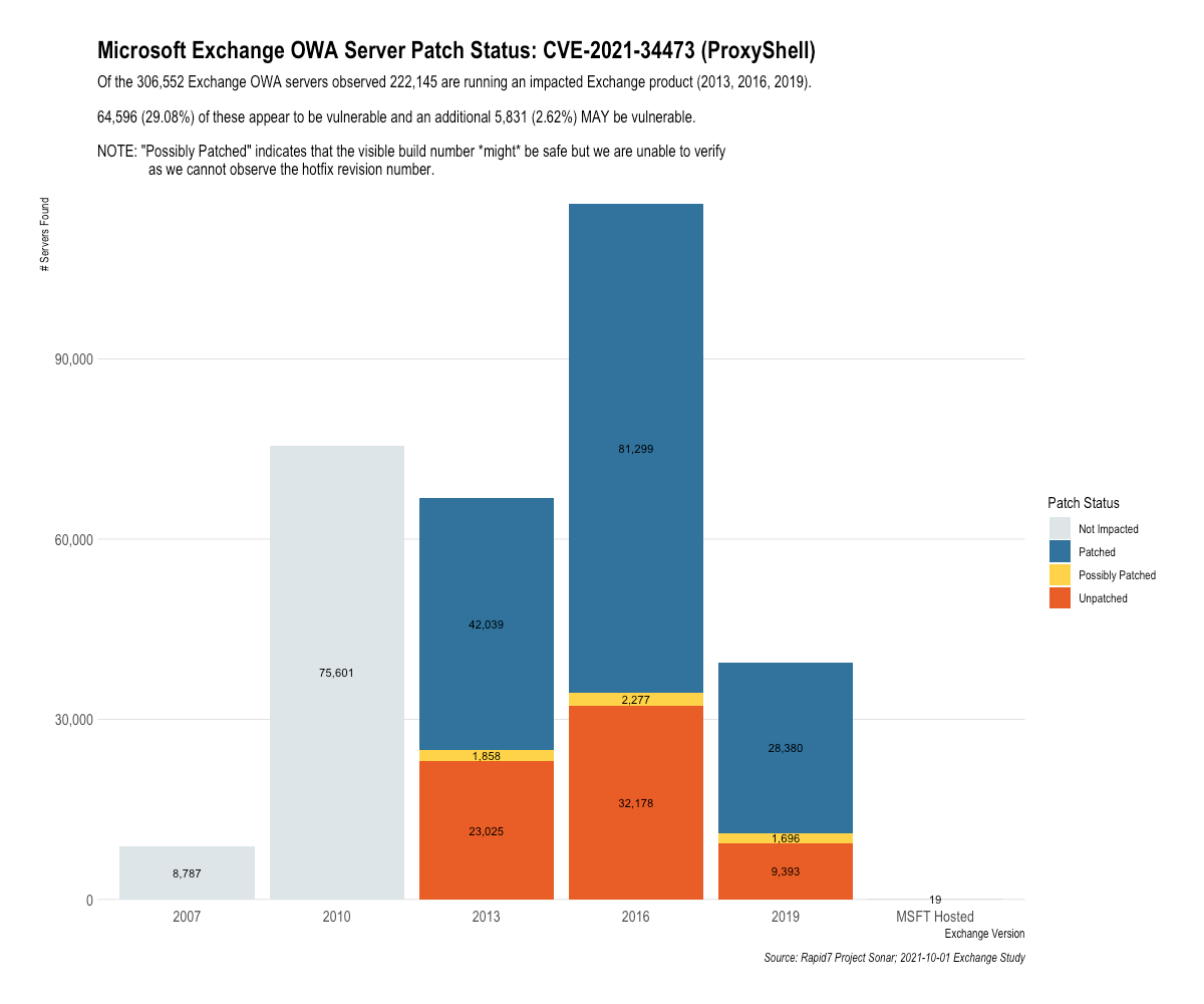
To put it another, starker way: 6 months after patches have been available for the ProxyLogon family of vulnerabilities, 1 in 3 impacted Exchange Servers are still susceptible to attacks using the ProxyShell method.
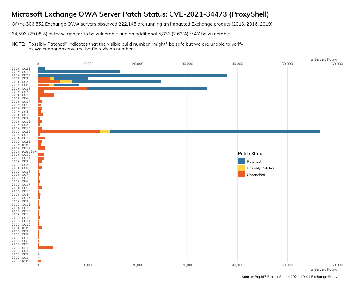
When we sort this data by the Exchange Server versions that organizations are using, we see the uncertainty in patch status tends to cluster around specific versions, particularly 2013 Cumulative Update 23.
We also pulled the server header for these instances with the goal of using the version of IIS as a proxy indicator of what OS the servers may be running — and we found an alarmingly large proportion of instances that were running end-of-life servers and/or operating systems, for which Microsoft no longer issues patch updates.
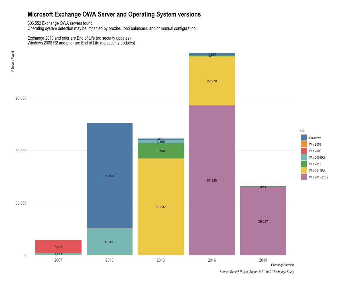
That group includes the two bars on the left of this graph, which represent 2007 and 2010 Exchange Server versions: 75,300 instances of 2010 and 8,648 instances of 2007 are still running out there on the internet, roughly 27% of all instances we observed. Organizations still operating these products can count themselves lucky that ProxyShell and ProxyLogon don’t impact these older versions of Exchange (as far as we know). But that doesn’t mean those companies are out of the woods — if you still haven’t replaced Exchange Server 2010, you’re probably also doing other risky things in your environment.
Looking ahead, the next group of products that will go end-of-life are the Windows Server 2012 and 2012 R2 operating systems, represented in green and yellow, respectively, within the graph. That means 92,641 instances of Exchange — nearly a third of all Exchange Servers on the internet — will be running unsupported operating systems for which Microsoft isn’t obligated to provide security fixes after they go end-of-life in 2023.
It’s a matter of when, not if, we encounter the next family of vulnerabilities that lets attackers have a field day with huge sets of sensitive data like those contained in Exchange Servers. And for companies that haven’t yet patched, ProxyShell and its related attack chains are still a real threat. Here’s what you can do now to proactively mitigate these vulnerabilities.
If you’re already a Rapid7 customer, there’s good news: InsightVM already has authenticated scans to detect these vulnerabilities, so users of the product should already have a good sense of where their Exchange environments stand. On the offensive side, your red teams and penetration testers can highlight the risk of running vulnerable Exchange instances with modules exercising ProxyLogon and ProxyShell. And as our research team continues to develop techniques for getting this kind of detailed information about exposures, we ensure our products know about those methods so they can more effectively help customers understand their vulnerabilities.
But for all of us, these vulnerabilities are a reminder that security requires a proactive mindset — and failing to cover the basics like upgrading to supported products and installing security updates leaves organizations at risk when a particularly thorny set of attack chains rears its head.
Post Syndicated from Wei Teh original https://aws.amazon.com/blogs/architecture/field-notes-build-a-cross-validation-machine-learning-model-pipeline-at-scale-with-amazon-sagemaker/
When building a machine learning algorithm, such as a regression or classification algorithm, a common goal is to produce a generalized model. This is so that it performs well on new data that the model has not seen before. Overfitting and underfitting are two fundamental causes of poor performance for machine learning models. A model is overfitted when it performs well on known data, but generalizes poorly on new data. However, an underfit model performs poorly on both trained and new data. A reliable model validation technique helps provide better assessment for predicting model performance in practice, and provides insight for training models to achieve the best accuracy.
Cross-validation is a standard model validation technique commonly used for assessing performance of machine learning algorithms. In general, it works by first sampling the dataset into groups of similar sizes, where each group contains a subset of data dedicated for training and model evaluation. After the data has been grouped, a machine learning algorithm will fit and score a model using the data in each group independently. The final score of the model is defined by the average score across all the trained models for performance metric representation.
There are few cross-validation methods commonly used, including k-fold, stratified k-fold, and leave-p-out, to name a few. Although there are well-defined data science frameworks that can help simplify cross-validation processes, such as Python scikit-learn library, these frameworks are designed to work in a monolithic, single compute environment. When it comes to training machine learning algorithms with large volume of data, these frameworks become bottlenecked with limited scalability and reliability.
In this blog post, we are going to walk through the steps for building a highly scalable, high-accuracy, machine learning pipeline, with the k-fold cross-validation method, using Amazon Simple Storage Service (Amazon S3), Amazon SageMaker Pipelines, SageMaker automatic model tuning, and SageMaker training at scale.
To operate the k-fold cross validation training pipeline at scale, we built an end to end machine learning pipeline using SageMaker native features. This solution implements the k-fold data processing, model training, and model selection processes as individual components to maximize parallellism. The pipeline is orchestrated through SageMaker Pipelines in distributed manner to achieve scalability and performance efficiency. Let’s dive into the high-level architecture of the solution in the following section.
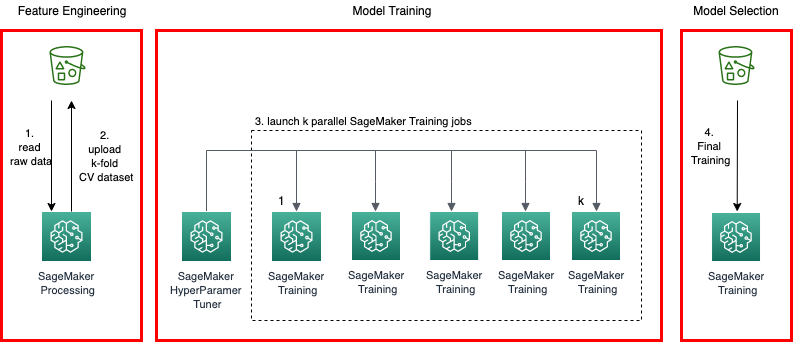
Figure 1. Solution architecture
The overall solution architecture is shown in Figure 1. There are four main building blocks in the k-fold cross-validation model pipeline:
The final output from the pipeline is a model that represents best performance and accuracy for the given dataset. The pipeline can be orchestrated easily using a workflow management tool, such as Pipelines.
Amazon SageMaker is a fully managed service that enables data scientists and developers to quickly develop, train, tune, and deploy machine learning quickly and at scale. When it comes to choosing the right machine learning and data processing frameworks to solve problems, SageMaker gives you the flexibility to use prebuilt containers bundled with the supported common machine learning frameworks—such as Tensorflow, Pytorch, and MxNet—or to bring your own container images with custom scripts and libraries that fit your use cases to train on the highly available SageMaker model training environment. Additionally, Pipelines enables users to develop complete machine learning workflows using python SDK, and manage these workflows in SageMaker Studio.
For simplicity, we will use the public Iris flower data as the train and test dataset to build a multivariate classification model using linear algorithm (SVM). The pipeline architecture is agnostic to the data and model; hence, it can be modified to adopt a different dataset or algorithm.
To deploy the solution, you require the following:
In this section, we are going to walk through the steps to create a cross-validation model training pipeline using Pipelines. The main components are as follows.
In this step, the original dataset is split into k equal-sized samples. One of the k samples is retained as the validation data for model evaluation, with the remaining k-1 samples to be used as training data. This process is repeated k times, with each of the k samples used as the validation set only one time. The k sample collections are uploaded to an S3 bucket, with the prefix corresponding to an index (0 – k-1) to be identified as the input path to the specified training jobs in the next step of the pipeline. The cross-validation split is submitted as a SageMaker processing job orchestrated through the Pipelines processing step. The processing flow is shown in Figure 2.
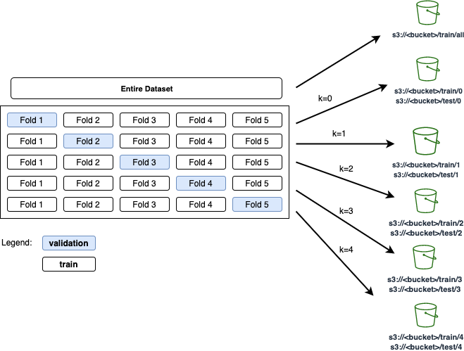
Figure 2. K-fold cross-validation: original data is split into k equal-sized samples uploaded to S3 bucket
The following code snippet splits the k-fold dataset in the preprocessing script:
def save_kfold_datasets(X, y, k):
    """ Splits the datasets (X,y) k folds and saves the output from
    each fold into separate directories.

    Args:
        X : numpy array represents the features
        y : numpy array represetns the target
        k : int value represents the number of folds to split the given datasets
    """

    # Shuffles and Split dataset into k folds.
    kf = KFold(n_splits=k, random_state=23, shuffle=True)

    fold_idx = 0
    for train_index, test_index in kf.split(X, y=y, groups=None):
       X_train, X_test = X[train_index], X[test_index]
       y_train, y_test = y[train_index], y[test_index]
       os.makedirs(f'{base_dir}/train/{fold_idx}', exist_ok=True)
       np.savetxt(f'{base_dir}/train/{fold_idx}/train_x.csv', X_train, delimiter=',')
       np.savetxt(f'{base_dir}/train/{fold_idx}/train_y.csv', y_train, delimiter=',')

       os.makedirs(f'{base_dir}/test/{fold_idx}', exist_ok=True)
       np.savetxt(f'{base_dir}/test/{fold_idx}/test_x.csv', X_test, delimiter=',')
       np.savetxt(f'{base_dir}/test/{fold_idx}/test_y.csv', y_test, delimiter=',')
fold_idx += 1In a typical cross-validation training scenario, a chosen algorithm is trained for k times with specific training and a validation dataset sampled through the k-fold technique, mentioned in the previous step. Traditionally, the cross-validation model training process is performed sequentially on the same server. This method is inefficient and doesn’t scale well for models with large volumes of data. Because all the samples are uploaded to an S3 bucket, we can now run k training jobs in parallel. Each training job will consume input samples in the specified bucket location correspond to the index (ranged between 0 – k-1) given to the training job. Additionally, the hyperparameter values must be the same for all k jobs because cross validation estimates the true out-of-sample performance of a model trained with this specific set of hyperparameters.
Although the cross-validation technique helps generalize the models, hyperparameter tuning for the model is typically performed manually. In this blog post, we are going to take a heuristic approach of finding the most optimized hyperparameters using SageMaker automatic model tuning.
We start by defining a training script that accepts the hyperparameters as input for the specified model algorithm, and then implement the model training and evaluation steps.
The steps involved in the training script are summarized as follows:
if __name__ == '__main__':
    parser = argparse.ArgumentParser()
    parser.add_argument('-c', '--c', type=float, default=1.0)
    parser.add_argument('--gamma', type=float)
    parser.add_argument('--kernel', type=str)
    # Sagemaker specific arguments. Defaults are set in the environment variables.
    parser.add_argument('--output-data-dir', type=str, default=os.environ['SM_OUTPUT_DATA_DIR'])
    parser.add_argument('--model-dir', type=str, default=os.environ['SM_MODEL_DIR'])
    parser.add_argument('--train', type=str, default=os.environ['SM_CHANNEL_TRAIN'])
    parser.add_argument('--test', type=str, default=os.environ.get('SM_CHANNEL_TEST'))
    args = parser.parse_args()
    model = train(train=args.train, test=args.test)
    evaluate(test=args.test, model=model)
    dump(model, os.path.join(args.model_dir, "model.joblib"))
Next, we create a python script that performs cross-validation model training by submitting k SageMaker training jobs in parallel with given hyperparameters. Additionally, the script monitors the progress of the training jobs, and calculates the objective metrics by averaging the scores across the completed jobs.
Now we create a python script that uses a SageMaker automatic model tuning job to find the optimal hyperparameters for the trained models. The hyperparameter tuner works by running a specified number of training jobs using the ranges of hyperparameters specified. The number of training jobs and ranges of hyperparameters are given in the input parameter to the script. After the tuning job completes, the objective metrics, as well as the hyperparameters from the best cross-validation model training job, are captured, formatted in JSON format, respectively, to be used in the next steps of the workflow. Figure 3 illustrates cross-validation training with automatic model tuning.

Figure 3. In cross-validation training step, a SageMaker HyperparameterTuner job invokes n training jobs. The metrics and hyperparameters are captured for downstream processes.
Finally, the training and cross-validation scripts are packaged and built as a custom container image, available for the SageMaker automatic model tuning job for submission. The following code snippet is for building the custom image:
FROM python:3.7
RUN apt-get update && pip install sagemaker boto3 numpy sagemaker-training
COPY cv.py /opt/ml/code/train.py
COPY scikit_learn_iris.py /opt/ml/code/scikit_learn_iris.py
ENV SAGEMAKER_PROGRAM train.pyfrom sagemaker.workflow.conditions import ConditionGreaterThanOrEqualTo
from sagemaker.workflow.condition_step import (
ConditionStep,
JsonGet,
)
cond_gte = ConditionGreaterThanOrEqualTo(
left=JsonGet(
step=step_cv_train_hpo,
property_file=evaluation_report,
json_path="multiclass_classification_metrics.accuracy.value",
),
right=baseline_model_objective_value,
)
step_cond = ConditionStep(
name="ModelEvaluationStep",
conditions=[cond_gte],
if_steps=[step_model_selection, step_register_model],
else_steps=[],
)from sagemaker.inputs import TrainingInput
from sagemaker.workflow.steps import TrainingStep
from sagemaker.sklearn.estimator import SKLearn
sklearn_estimator = SKLearn("scikit_learn_iris.py",
framework_version=framework_version,
instance_type=training_instance_type,
py_version='py3',
source_dir="code",
output_path=s3_bucket_base_path_output,
role=role)
step_model_selection = TrainingStep(
name="ModelSelectionStep",
estimator=sklearn_estimator,
inputs={
"train": TrainingInput(
s3_data=f'{step_process.arguments["ProcessingOutputConfig"]["Outputs"][0]["S3Output"]["S3Uri"]}/all',
content_type="text/csv"
),
"jobinfo": TrainingInput(
s3_data=f"{s3_bucket_base_path_jobinfo}",
content_type="application/json"
)
}
)In the final step of the pipeline, we are going to register the trained model with Model Registry by associating model objective metrics, the model artifact location on S3 bucket, the estimator object used in the model selection step, model training and inference metadata, and approval status. The following code snippet illustrates the model registry step using ModelMetrics and RegisterModel.
from sagemaker.model_metrics import MetricsSource, ModelMetrics
from sagemaker.workflow.step_collections import RegisterModel
model_metrics = ModelMetrics(
    model_statistics=MetricsSource(
        s3_uri="{}/evaluation.json".format(
            step_cv_train_hpo.arguments["ProcessingOutputConfig"]["Outputs"][0]["S3Output"]["S3Uri"]
        ),
        content_type="application/json",
    )
)
step_register_model = RegisterModel(
    name="RegisterModelStep",
    estimator=sklearn_estimator,
    model_data=step_model_selection.properties.ModelArtifacts.S3ModelArtifacts,
    content_types=["text/csv"],
    response_types=["text/csv"],
    inference_instances=["ml.t2.medium", "ml.m5.xlarge"],
    transform_instances=["ml.m5.xlarge"],
    model_package_group_name=model_package_group_name,
    approval_status=model_approval_status,
    model_metrics=model_metrics,
Figure 4 shows a model version registered in SageMaker Model Registry upon a successful pipeline job through Studio.
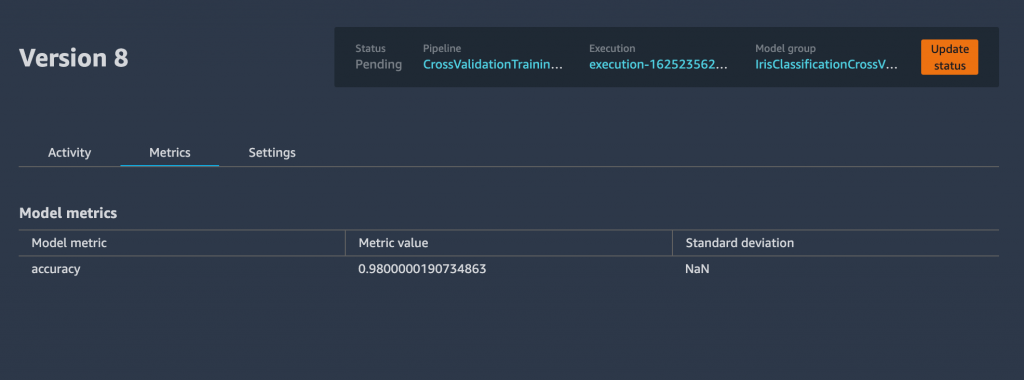
Figure 4. Model version registered successfully in SageMaker
from sagemaker.workflow.pipeline_experiment_config import PipelineExperimentConfig
from sagemaker.workflow.execution_variables import ExecutionVariables
pipeline_name = f"CrossValidationTrainingPipeline"
pipeline = Pipeline(
    name=pipeline_name,
    parameters=[
        processing_instance_count,
        processing_instance_type,
        training_instance_type,
        training_instance_count,
        inference_instance_type,
        hpo_tuner_instance_type,
        model_approval_status,
        role,
        default_bucket,
        baseline_model_objective_value,
        bucket_prefix,
        image_uri,
        k,
        max_jobs,
        max_parallel_jobs,
        min_c,
        max_c,
        min_gamma,
        max_gamma,
        gamma_scaling_type
    ],
    pipeline_experiment_config=PipelineExperimentConfig(
      ExecutionVariables.PIPELINE_NAME,
      ExecutionVariables.PIPELINE_EXECUTION_ID),
    steps=[step_process, step_cv_train_hpo, step_cond],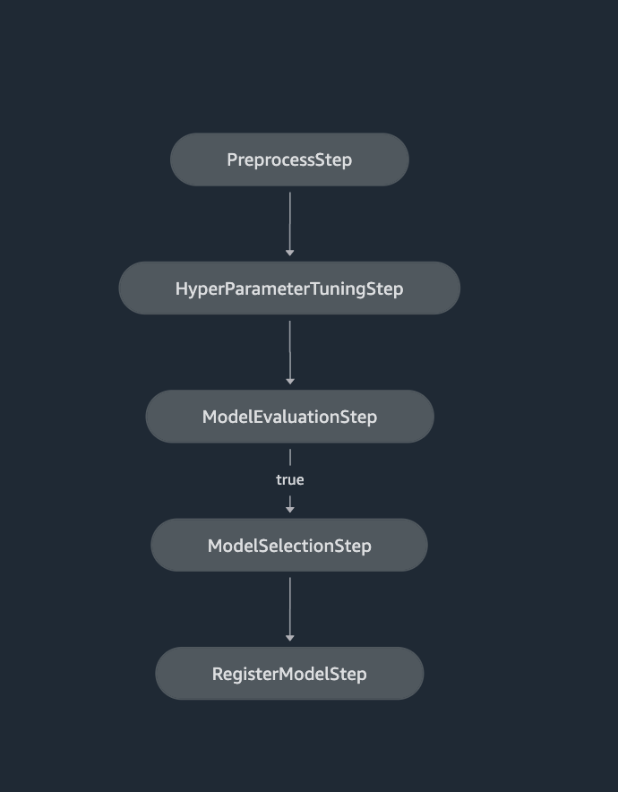
Figure 5. SageMaker Pipelines definition shown in SageMaker Studio
Finally, to kick off the pipeline, invoke the pipeline.start() function, with optional parameters specific to the job run:
execution = pipeline.start(
    parameters=dict(
        BaselineModelObjectiveValue=0.8,
        MinimumC=0,
        MaximumC=1
    ))
You can track the pipeline job from within Studio, or use SageMaker application programming interfaces (APIs). Figure 6 shows a screenshot of a pipeline job in progress from Studio.
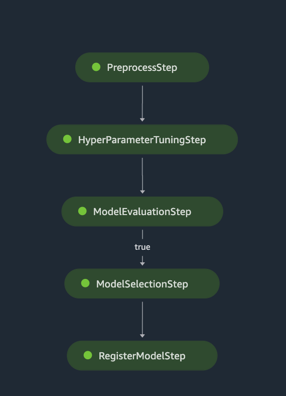
Figure 6. SageMaker Pipelines job progress shown in SageMaker Studio
In this blog post, we showed you an architecture that orchestrates a complete workflow for cross-validation model training. We implemented the workflow using SageMaker Pipelines that incorporates preprocessing, hyperparameter tuning, model evaluation, model selection, and model registration. The solution addresses the common challenge of orchestrating cross-validation model pipeline at scale. The entire pipeline implementation, including a jupyter notebook that defines the pipeline, a Dockerfile and python scripts described in this blog post, can be found in the GitHub project.
Post Syndicated from Dina Kozlov original https://blog.cloudflare.com/staging-tls-certificate-every-deployment-safe-deployment/


We are excited to announce that Enterprise customers now have the ability to test custom uploaded certificates in a staging environment before pushing them to production.
If you’re running a website or the API that’s behind a popular app, you know your users have high expectations: it can’t just be up and running; it also has to be fast and secure. One of the easiest and most standardized ways to secure connections is with the TLS protocol. To do that, you need to acquire a TLS certificate for your domain.
One way to get a certificate is by using a CDN provider, like Cloudflare. We make the process really easy by issuing certificates on your behalf. Not just that, but when your certificate is getting closer to its expiration date, we are responsible for re-issuing it. But, if you don’t want Cloudflare to issue the certificate on your behalf and want to obtain the certificate yourself, you can do so. You can either keep control of your private key, or generate a Certificate Signing Request (CSR) through Cloudflare, so we maintain the private key, but you can still use the certificate authority (CA) of your choice for the certificate. Once you get your certificate, you upload it to Cloudflare and voilà — your site is secure.
One of the downsides of obtaining your own certificate is that you’re in charge of its renewal, which comes with a great deal of responsibility. You have to ensure that any renewed certificate will not cause TLS errors, causing your property to be unreachable by your users.
Now, you’re probably wondering, why is this so risky? What could go wrong?
It’s possible that when you renew a certificate, you forget to include one of your subdomains in the certificate. Another reason why your clients might see failures when you upload the new certificate is that some of those clients are pinning the old certificate.
Certificate pinning allows Internet application owners to say “trust this certificate and no other” by pinning the certificate or public key to their service, or even to client devices. While this was originally intended to tighten security, certificate pinning has created many problems. We have seen customers shoot themselves in the foot with certificate pinning numerous times. There are a lot of things that could go wrong: you could pin the wrong certificate, or configure the wrong settings, which will bring your service down. It’s possible that you rely on a CDN for your certificate renewal and forgot to update your pin — again, blocking access to your service in the process. Alternatively, you can pin certificates to clients so that they refuse connections from servers that don’t have the same certificate. But when it comes to renewing that certificate, you have to make sure that your clients have the updated certificate, or they won’t be able to access your server. Instead, you can use tools like Cloudflare’s Certificate Transparency Monitoring which notifies you when certificates are being issued for your domain.
But, some of our customers do rely on this behavior. So for them, switching to a new certificate is a big change — one that can bring down their whole application. For this reason, they need to be able to test the new certificate to identify any problems that may occur before their customers see it.
When it comes to your traffic, there are things you can’t predict. You can’t control if your customer’s browser is having a bad day, or if some ISP is having a network outage. When it comes to certificate deployment, the last thing you want is to be surprised. Imagine pushing out a new certificate, and realizing you’ve uploaded the wrong one only after customers complain they’ve lost access; or that you never updated your pin to your new certificate to begin with. Mistakes happen, but this type of outage can cause a lot of pain and lose you a lot of money and trust. The good news is that this is preventable.
We are giving customers the ability to find these problems before they’re encountered by real users. We’re doing this by giving customers the ability to test certificate deployment changes against a pair of staging IPs.
Imagine uploading a new certificate, finding any related problems, and fixing them in a way that doesn’t impact production traffic. That’s exactly what Staging Certificates allows you to do!
You can go to the Staging Certificates section under the SSL/TLS tab in the Cloudflare dashboard and upload a new certificate to our staging network. The staging network will replicate your production environment but will only be accessible through the Staging IPs.
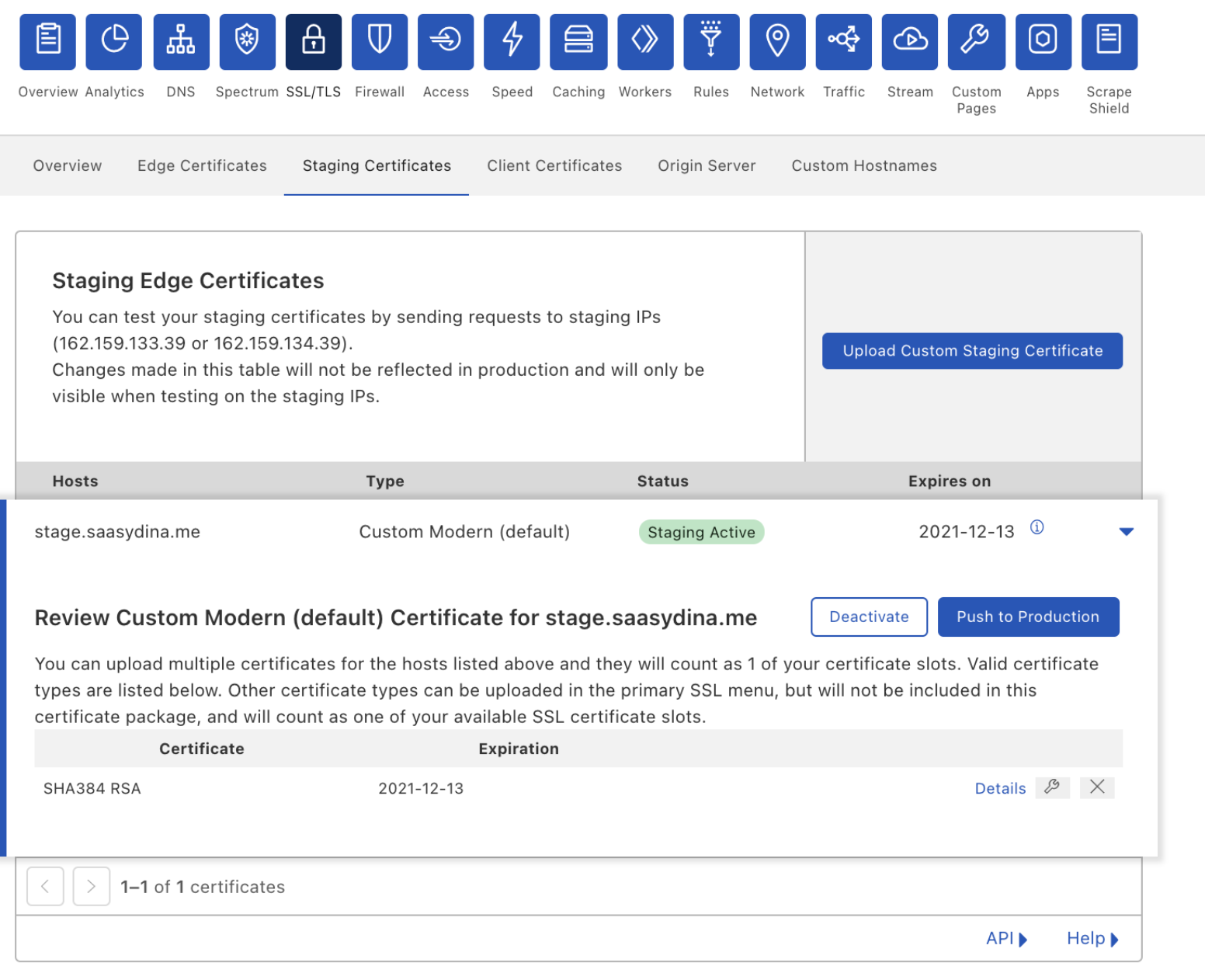
Once you upload your certificate, you can make `curl` requests against the staging IPs to verify that it’s being served and that it covers all the hostnames that you need it to. If you’ve decided to pin your previous certificate, the staging environment helps you verify that your pins have been updated correctly and that TLS termination is successful.
Once you’re confident in your tests, you can push the certificate out to production.
Mistakes happen. It’s possible that you found one client device whose pin you forgot to update. In that case, you can disable the certificate to quickly mitigate the problem by rolling back to the certificate that you were last serving.
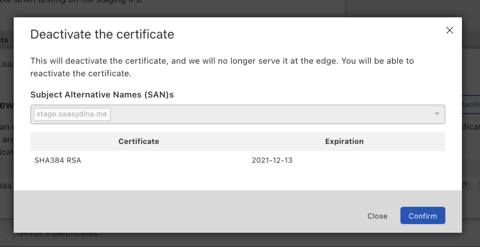
What if you realize that this is a bigger issue, and you need more time to test? You can push the disabled certificate back to the staging environment, and when you’ve verified everything works correctly, push it back to production.
We want to de-risk every change you make. Staging your custom uploaded certificates is a start, but it doesn’t end there. In the future, we’ll allow you to stage certificate renewals for certificates issued through Cloudflare. We’re also planning to give customers the ability to test TLS configuration changes like minimum TLS or cipher suite settings.
If you’re interested in staying aware of these future developments, or you have some settings that you want to test in staging, reach out to your Account team and let them know!
This feature is currently in Beta and available to Enterprise customers. If you want to use it, reach out to your Account team to get it enabled.
Post Syndicated from The History Guy: History Deserves to Be Remembered original https://www.youtube.com/watch?v=KSU1-5_6byI
Post Syndicated from Philip Colligan original https://www.raspberrypi.org/blog/introducing-raspberrypicom/
I am delighted to announce the launch of raspberrypi.com — a new website dedicated to Raspberry Pi computers and associated technologies. Head on over to find all about our low-cost, high-performance PCs, add-on boards or HATs, microcontrollers, accessories, and much more.
As well as being able to learn about and purchase the full range of hardware products, on the new website you can download our latest software, find detailed technical documentation, connect with the community on the forums, and read the latest news about Raspberry Pi technologies and how they’re being used to change the world.
This website (raspberrypi.org) will continue to be the home for the Raspberry Pi Foundation and all of our educational initiatives to help young people learn about computers and how to create with digital technologies.
That includes online resources to help young people learn how to code, information about our networks of Code Clubs and CoderDojos, training and support for teachers and other educators, and access to the world’s leading-edge research into computing education.
You’ll still be able to find loads of resources about Raspberry Pi computers in education, and cool opportunities for young people to learn how to code and create with Raspberry Pi technologies, whether that’s our space programme Astro Pi, or building robots with Raspberry Pi Pico.
When raspberrypi.org was first launched as a WordPress blog in 2011, we were talking about a low-cost, programmable computer that was being designed for education.
Fast-forward a decade, and we are now speaking about an increasingly broad range of technology and education products and services to industry, hobbyists, educators, researchers, and young people. While there is lots of overlap between those communities and their interests, it is becoming increasingly difficult to address everyone’s needs on one website. So this change is really all about making life easier for you.
We will continue to provide lots of links and connections between the two sites to make sure that you can easily find what you’re looking for. As ever, we’d love to hear your feedback in the comments below.
Alongside the changes to the websites, we’re also launching new social channels that are focused on the Foundation’s educational initiatives. We look forward to seeing you there.
The post Introducing raspberrypi.com appeared first on Raspberry Pi.
Post Syndicated from Bozho original https://techblog.bozho.net/hypotheses-about-what-happened-to-facebook/
Facebook was down. I’d recommend reading Cloudflare’s summary. Then I recommend reading Facebook’s own account on the incident. But let me expand on that. Facebook published announcements and withdrawals for certain BGP prefixes which lead to removing its DNS servers from “the map of the internet” – they told everyone “the part of our network where our DNS servers are doesn’t exist”. That was the result of a backbone self-inflicted failure due to a bug in the auditing tool that checks whether the commands executed aren’t doing harmful things.
Facebook owns a lot of IPs. According to RIPEstat they are part of 399 prefixes (147 of them are IPv4). The DNS servers are located in two of those 399. Facebook uses a.ns.facebook.com, b.ns.facebook.com, c.ns.facebook.com and d.ns.facebook.com, which get queries whenever someone wants to know the IPs of Facebook-owned domains. These four nameservers are served by the same Autonomous System from just two prefixes – 129.134.30.0/23 and 185.89.218.0/23. Of course “4 nameservers” is a logical construct, there are probably many actual servers behind that (using anycast).
I wrote a simple “script” to fetch all the withdrawals and announcements for all Facebook-owned prefixes (from the great API of RIPEstats). Facebook didn’t remove itself from the map entirely. As CloudFlare points out, it was just some prefixes that are affected. It can be just these two, or a few others as well, but it seems that just a handful were affected. If we sort the resulting CSV from the above script by withdrawals, we’ll notice that 129.134.30.0/23 and 185.89.218.0/23 are the pretty high up (alongside 185.89 and 123.134 with a /24, which are all included in the /23). Now that perfectly matches Facebook’s account that their nameservers automatically withdraw themselves if they fail to connect to other parts of the infrastructure. Everything may have also been down, but the logic for withdrawal is present only in the networks that have nameservers in them.
So first, let me make three general observations that are not as obvious and as universal as they may sound, but they are worth discussing:
The main explanation is the accidental outage. This is what Facebook engineers explain in the blogpost and other accounts, and that’s what seems to have happened. However, there are alternative hypotheses floating around, so let me briefly discuss all of the options.
Distinguishing between the three options is actually hard. You can mask a deliberate outage as an accident, a malicious actor can make it look like a deliberate self-sabotage. That’s why there are speculations. To me, however, by all of the data we have in RIPEStat and the various accounts by CloudFlare, Facebook and other experts, it seems that a chain of mistakes (operational and possibly design ones) lead to this.
The post Hypotheses About What Happened to Facebook appeared first on Bozho's tech blog.
Post Syndicated from Explosm.net original http://explosm.net/comics/5995/
New Cyanide and Happiness Comic
Post Syndicated from The Hook Up original https://www.youtube.com/watch?v=ULVcpqC2NU4
Post Syndicated from original https://xkcd.com/2525/

Post Syndicated from original https://lwn.net/Articles/871195/rss
Two Google engineers came to Open
Source Summit North America 2021 to talk about a project to change the
way the company creates and maintains the kernel it runs in its data
centers on its production
systems. Andrew Delgadillo and Dylan Hatch described the current production
kernel (Prodkernel) and the problems that occur because it is so far from
the mainline. Project Icebreaker is an effort to change that and to
provide a near-mainline kernel for development and testing within Google;
the talk looked at the project, its risks, its current status, and its plans.
Post Syndicated from original https://lwn.net/Articles/871992/rss
The Asahi Linux project has a progress
report on its goal of running Linux on Mac M1 hardware.
Earlier this year we saw the absolute lowest level drivers being merged into the kernel. Those are important for bring-up, but to get a usable system we need many more. Over September we’ve seen a lot of action on this front, with many important drivers now in review or even already merged for Linux 5.16. The goal of the Asahi Linux project is to upstream everything into the Linux kernel, so all our drivers are eventually headed for upstream review.
Post Syndicated from original https://lwn.net/Articles/871985/rss
The AlmaLinux Foundation has opened
membership to everyone.
The AlmaLinux Foundation […] was created as a 501(c)(6) non-profit (the same as the Linux Foundation) in order to put OWNERSHIP of the OS, the Intellectual Property and the direction of the project into the hands of the community. By joining as a member (100% free for community members) you have the right and the ability to vote on board members and the direction of the project and other decisions as they will come up in the future.
Post Syndicated from Chinmayi Narasimhadevara original https://aws.amazon.com/blogs/big-data/query-your-amazon-msk-topics-interactively-using-amazon-kinesis-data-analytics-studio/
Amazon Kinesis Data Analytics Studio makes it easy to analyze streaming data in real time and build stream processing applications powered by Apache Flink using standard SQL, Python, and Scala. With a few clicks on the AWS Management Console, you can launch a serverless notebook to query data streams and get results in seconds. Kinesis Data Analytics reduces the complexity of building and managing Apache Flink applications. Apache Flink is an open-source framework and engine for processing data streams. It’s highly available and scalable, delivering high throughput and low latency for stream processing applications.
If you’re running Apache Flink workloads, you may experience the non-trivial challenge of developing your distributed stream processing applications without having true visibility into the steps your application performs for data processing. Kinesis Data Analytics Studio combines the ease of use of Apache Zeppelin notebooks with the power of the Apache Flink processing engine to provide advanced streaming analytics capabilities in a fully managed offering. This accelerates developing and running stream processing applications that continuously generate real-time insights.
In this post, we introduce you to Kinesis Data Analytics Studio and how to get started querying data interactively from an Amazon Managed Streaming for Kafka (Amazon MSK) cluster using SQL, Python, and Scala. We also demonstrate how to query data across different topics using Kinesis Data Analytics Studio. Kinesis Data Analytics Studio is also compatible with Amazon Kinesis Data Streams, Amazon Simple Storage Service (Amazon S3), and a variety of other data sources supported by Apache Flink.
To get started, you must have the following prerequisites:
To follow this guide and interact with your streaming data, you need a data stream with data flowing through.
You can create your Kafka cluster either using the Amazon MSK console or the following AWS Command Line Interface (AWS CLI) command. For console instructions, see Getting Started Using Amazon MSK and creating Studio notebook with MSK
You can either create topics and messages or use existing topics in the MSK cluster.
For this post, we have two topics in the MSK cluster, impressions and clicks, and they have the following fields in JSON format:
bid_id, campaign_id, country_code, creative_details, i_timestampcorrelation_id, tracker, c_timestampThe correlation_id is the click correlation ID for a bid_id, so the field has common values across topics that we use for the join.
For the data in the MSK topic, we use the Amazon MSK Data Generator. Refer to the GitHub repo for setup and usage details. (We will be using the adtech.json sample for this blog)
The following are sample JSON records generated for the impressions topic:
The following are sample JSON records generated for the clicks topic:
You can start interacting with your data stream by following these simple steps:
You can create a custom role for specific use cases on the IAM console.
We keep the default settings for the application and can scale up as needed.
To connect to an MSK cluster, you must specify the same VPC, subnets, and security groups for the Kinesis Data Analytics Studio notebook as were used to create the MSK cluster. If you chose Process data in real time during your setup, this is already set for you.
The Studio notebook is created with an IAM role for the notebook that grants the necessary access for the AWS Glue Data Catalog and tables.
Apache Zeppelin supports the Apache Flink interpreter and allows for the use of Apache Flink directly within Zeppelin for interactive data analysis. Within the Flink interpreter, three languages are supported as of this writing: Scala, Python (PyFlink), and SQL. The notebook requires a specification to one of these languages at the top of each paragraph in order to interpret the language properly:
There are several other predefined variables per interpreter, such as the senv variable in Scala for a StreamExecutionEnvironment, or st_env in Python for the same. You can review the full list of these entry point variables.
In this section, we show the same example code in all three languages to highlight the flexibility Zeppelin affords you for development.
We use the %flink.ssql(type=update) header to signify to the notebook that this paragraph will be interpreted as Flink SQL. We create two tables from the Kafka topics:
bid_id, campaign_id, creative_details, country_code, and i_timestamp columns providing details of impressions in the systemcorrelation_id, tracker, and c_timestamp providing details of the clicks for an impression.The tables use the Kafka connector to read from a Kafka topic called impressions and clicks in the us-east-1 Region from the latest offset.
As soon as this statement runs within a Zeppelin notebook, AWS Glue Data Catalog tables are created according to the declaration specified in the create statement, and the tables are available immediately for queries from the MSK cluster.
You don’t need to complete this step if your AWS Glue Data Catalog already contains the tables.
The following screenshot is the AWS Glue Data Catalog view, which shows the tables that represent MSK topics.
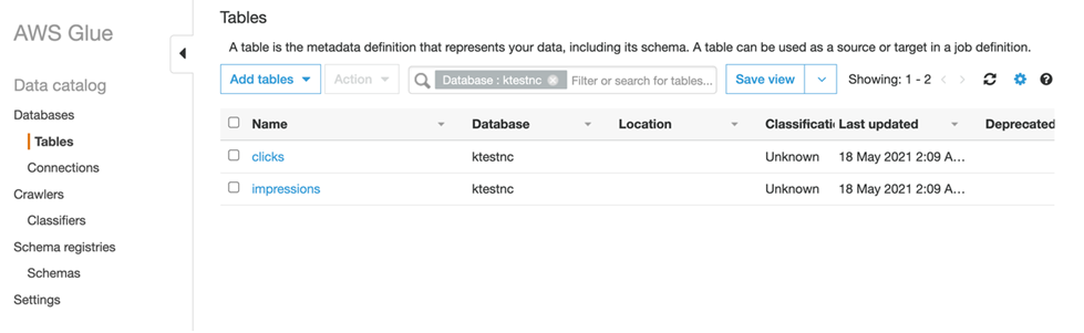
In the preceding tables, WATERMARK FOR serve_time AS serve_time - INTERVAL '5' SECOND means that we can tolerate out-of-order delivery of events in the timeframe of 5 seconds and still produce correct results.
After you create the tables, run a query that calculates the number of impressions within a tumbling window of 60 seconds broken down by campaign_id and creative_details:
The results from this query appear as soon as results are available.

Additionally, we want to see the clickthrough rate of the impressions:
This query produces one row for each impression and matches it with a click (if any) that was observed within 2 minutes after serving the ad. This is essentially performing a join operation across the topics to get this information.

You can insert this data back into an existing Kafka topic using the following code:
Create the corresponding table for the Kafka topic in the Data Catalog if it doesn’t exist already. After you run the preceding query, you can see data in your Amazon MSK topic (see the following sample below):
This is the CSV data from the preceding query, which shows the ClickThroughRate for the impressions. You can use this mechanism to store data back persistently into Kafka from Flink directly.
We use the %flink header to signify that this code block will be interpreted via the Scala Flink interpreter, and create a table identical to the one from the SQL example. However, in this example, we use the Scala interpreter’s built-in streaming table environment variable, stenv, to run a SQL DDL statement. If the table already exists in the AWS Glue Data Catalog, this statement issues an error stating that the table already exists.
Performing a tumbling window in the Scala table API first requires the definition of an in-memory reference to the table we created. We use the stenv variable to define this table using the from function and referencing the table name. After this is created, we can create a windowed aggregation over 1 minute of data, serve_time column. See the following code:
Use the ZeppelinContext to visualize the Scala table aggregation within the notebook:
The following screenshot shows our results.


Additionally, we want to see the clickthrough rate of the impressions by joining with the clicks:
Use the ZeppelinContext to visualize the Scala table aggregation within the notebook.
The following screenshot shows our results.


We use the %flink.pyflink header to signify that this code block will be interpreted via the Python Flink interpreter, and create a table identical to the one from the SQL and Scala examples. In this example, we use the Python interpreter’s built-in streaming table environment variable, st_env, to run a SQL DDL statement. If the table already exists in the AWS Glue Data Catalog, this statement issues an error stating that the table already exists.
Performing a sliding (hopping) window in the Python table API first requires the definition of an in-memory reference to the table we created. We use the st_env variable to define this table using the from_path function and referencing the table name. After this is created, we can create a windowed aggregation over 1 minute of data, emitting results every 5 seconds according to the event_time column. See the following code:
Use the ZeppelinContext to visualize the Python table aggregation within the notebook:
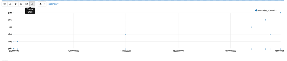
The following screenshot shows our results.

Additionally, we want to see the clickthrough rate of the impressions by joining with the clicks:
A Studio notebook consists of one or more tasks. You can split a Studio notebook task into several parallel instances to run, where each parallel instance processes a subset of the task’s data. The number of parallel instances of a task is called its parallelism, and adjusting that helps run your tasks more efficiently.
On creation, Studio notebooks are given four parallel Kinesis Processing Units (KPUs), which make up the application parallelism. To increase that parallelism, navigate to the Kinesis Data Analytics console, choose your application name, and choose the Configuration tab.

From this page, in the Scaling section, choose Edit and modify the Parallelism entry. We don’t recommend increasing the Parallelism Per KPU setting higher than 1 unless your application is I/O bound.
Choose Save changes to increase or decrease your application’s parallelism.
You may want to clean up the demo environment when you are done, To do so, stop the Studio notebook and delete the resources created for the Data Generator and the Amazon MSK cluster ( if you created a new cluster).
Kinesis Data Analytics Studio makes developing stream processing applications using Apache Flink much faster, with rich visualizations, a scalable and user-friendly interface to develop pipelines, and the flexibility of language choice to make any streaming workload performant and powerful. You can run paragraphs from within the notebook or promote your Studio notebook to a Kinesis Data Analytics for Apache Flink application with a durable state, as shown in the SQL example in this post.
For more information, see the following resources:
 Chinmayi Narasimhadevara is a Solutions Architect focused on Big Data and Analytics at Amazon Web Services. Chinmayi has over 15 years of experience in information technology. She helps AWS customers build advanced, highly scalable and performant solutions
Post Syndicated from Xiaozang Li original https://aws.amazon.com/blogs/architecture/connect-amazon-s3-file-gateway-using-aws-privatelink-for-amazon-s3/
AWS Storage Gateway is a set of services that provides on-premises access to virtually unlimited cloud storage. You can extend your on-premises storage capacity, and move on-premises backups and archives to the cloud. It provides low-latency access to cloud storage by caching frequently accessed data on premises, while storing data securely and durably in the cloud. This simplifies storage management and reduces costs for hybrid cloud storage use.
You may have privacy and security concerns with sending and receiving data across the public internet. In this case, you can use AWS PrivateLink, which provides private connectivity between Amazon Virtual Private Cloud (VPC) and other AWS services.
In this blog post, we will demonstrate how to take advantage of Amazon S3 interface endpoints to connect your on-premises Amazon S3 File Gateway directly to AWS over a private connection. We will also review the steps for implementation using the AWS Management Console.
Storage Gateway offers four different types of gateways to connect on-premises applications with cloud storage.
We will illustrate the use of Amazon S3 File Gateway in this blog.
AWS PrivateLink provides two types of VPC endpoints that you can use to connect to Amazon S3; Interface endpoints and Gateway endpoints. An interface endpoint is an elastic network interface with a private IP address. It serves as an entry point for traffic destined to a supported AWS service or a VPC endpoint service. A gateway VPC endpoint uses prefix lists as the IP route target in a VPC route table and supports routing traffic privately to Amazon S3 or Amazon DynamoDB. Both these endpoints securely connect to Amazon S3 over the Amazon network, and your network traffic does not traverse the internet.
Previously, AWS Storage Gateway did not support PrivateLink for Amazon S3 and Amazon S3 Access Points. Customers had to build and manage an HTTP proxy infrastructure within their VPC to connect their on-premises applications privately to S3 (see Figure 1). This infrastructure acted as a proxy for all the traffic originating from on-premises gateways to Amazon S3 through Amazon S3 Gateway endpoints. This setup would result in additional configuration and operational overhead. The HTTP proxy could also become a network performance bottleneck.
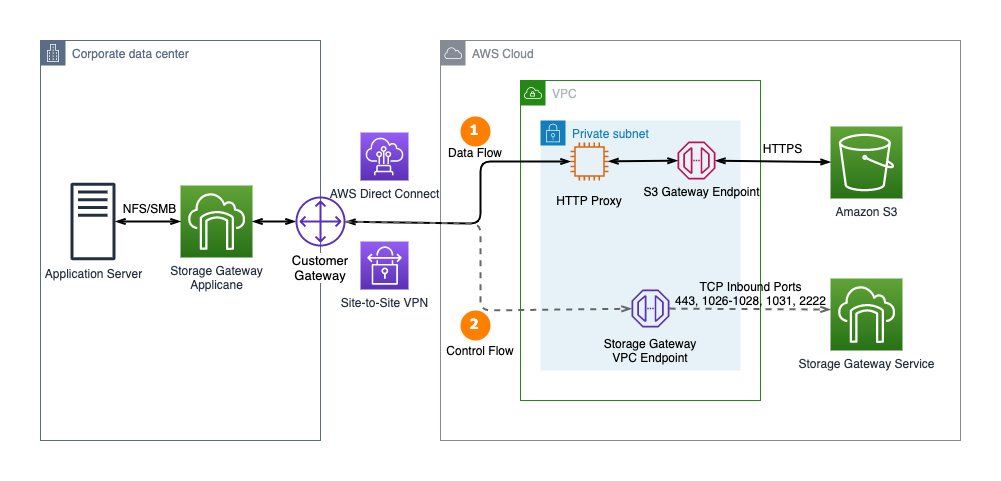
Figure 1. Connect to Amazon S3 Gateway endpoint using an HTTP proxy
AWS Storage Gateway recently added support for AWS PrivateLink for Amazon S3 and Amazon S3 Access Points. Customers can now connect their on-premises Amazon S3 File Gateway directly to Amazon S3 through a private connection. This uses an Amazon S3 interface endpoint and doesn’t require an HTTP proxy. Additionally, customers can use Amazon S3 Access Points instead of bucket names to map file shares. This enables more granular access controls for applications connecting to AWS Storage Gateway file shares (see Figure 2).
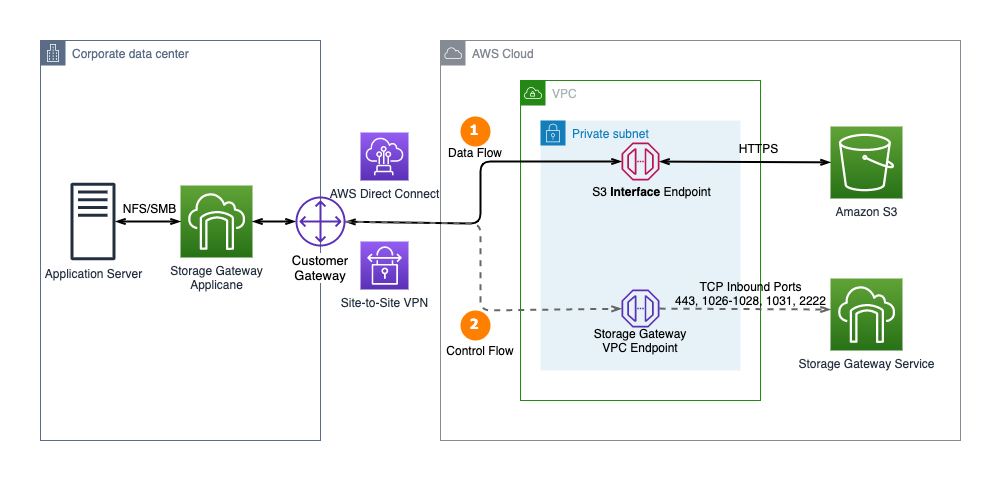
Figure 2. AWS Storage Gateway now supports AWS PrivateLink for Amazon S3 endpoints and Amazon S3 Access Points
Let’s look at how to create an Amazon S3 File Gateway file share, which is associated with a Storage Gateway. This file share stores data in an Amazon S3 bucket. It uses AWS PrivateLink for Amazon S3 to transfer data to the S3 endpoint.
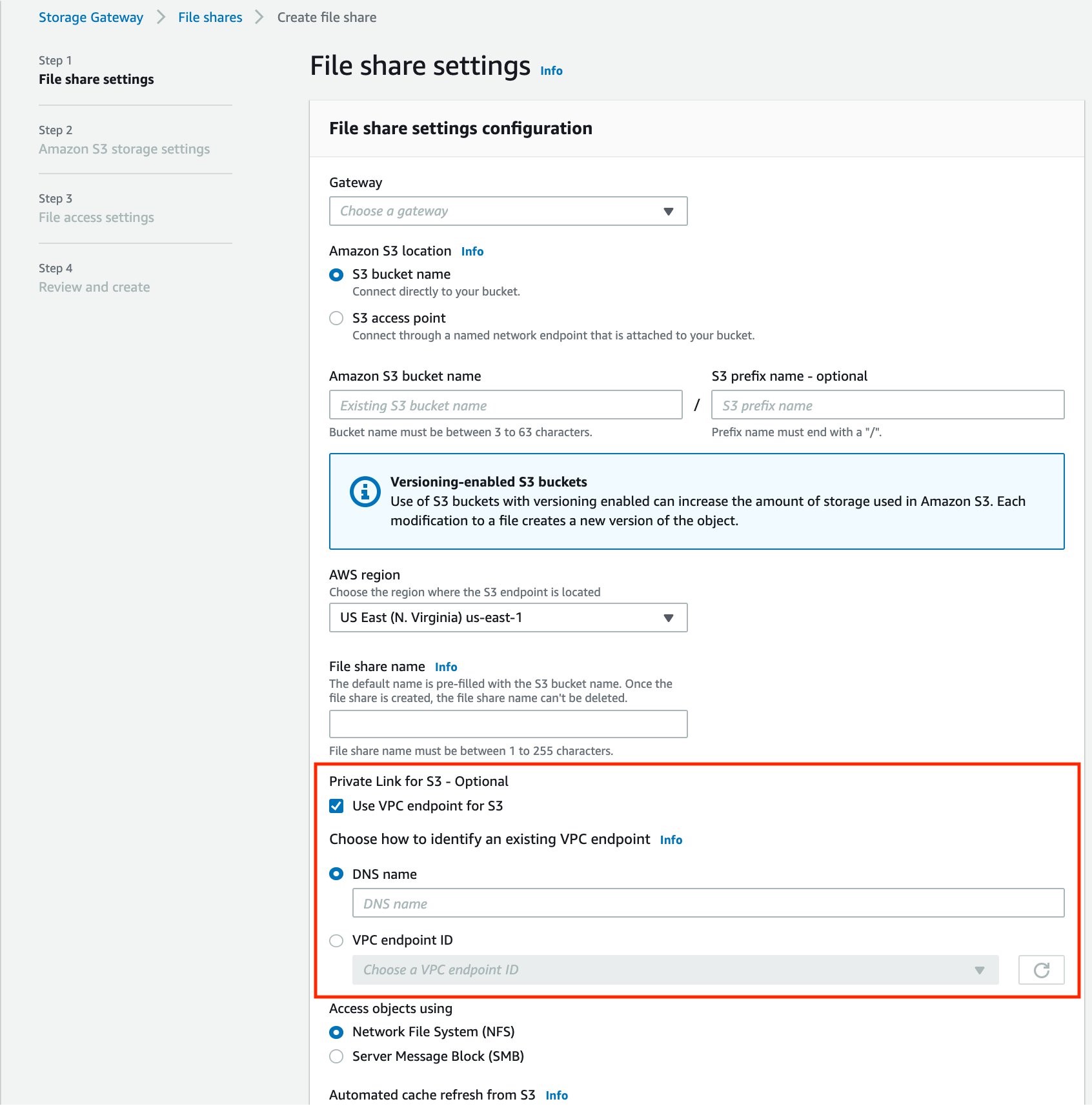
Figure 3. Create file share using VPC endpoints for Amazon S3
Best practices:
Be aware of PrivateLink pricing when using an S3 interface endpoint. The cost for each interface endpoint is based on usage per hour, the number of Availability Zones used, and the volume of data transferred over the endpoint. Additionally, each Amazon S3 VPC interface endpoint can be shared among multiple S3 File Gateways. Each file share associated with the Storage Gateway can be configured with or without PrivateLink. For workloads that do not need the private network connectivity, you can save on interface endpoints costs by creating a file share without PrivateLink.
Once you have set up an S3 File Gateway file share using PrivateLink for S3, you can verify that traffic is flowing over your private connectivity as follows:
1. Enable VPC Flow Log for the VPC hosting the S3 Interface endpoint. This also hosts the Virtual Private Gateway (VGW), which connects to the on-premises environment.
2. From your workstation, connect to your on-premises File Gateway over SMB or NFS protocol and upload a new file (see Figure 4).
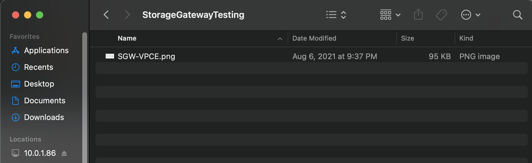
Figure 4. Upload a sample file to on-premises Storage Gateway
3. Navigate to the S3 bucket associated with the file share. After a few seconds, you should see that the new file has been successfully uploaded and appears in the S3 bucket (see Figure 5).
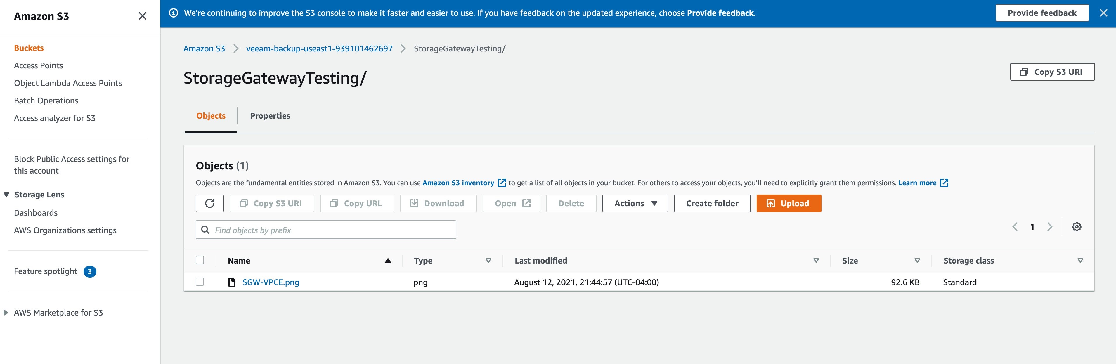
Figure 5. Verify that the sample file is uploaded to storage bucket
4. On the VPC flow log, look for the generated log events. You’ll see your S3 interface endpoint elastic network interface, your file gateway IP, Amazon S3 private IP, and port number, as shown in Figure 6. This verifies that the file was transferred over the private connection. If you do not see an entry, verify if the VPC Flow Logs have been enabled on the correct VPC and elastic network interface.
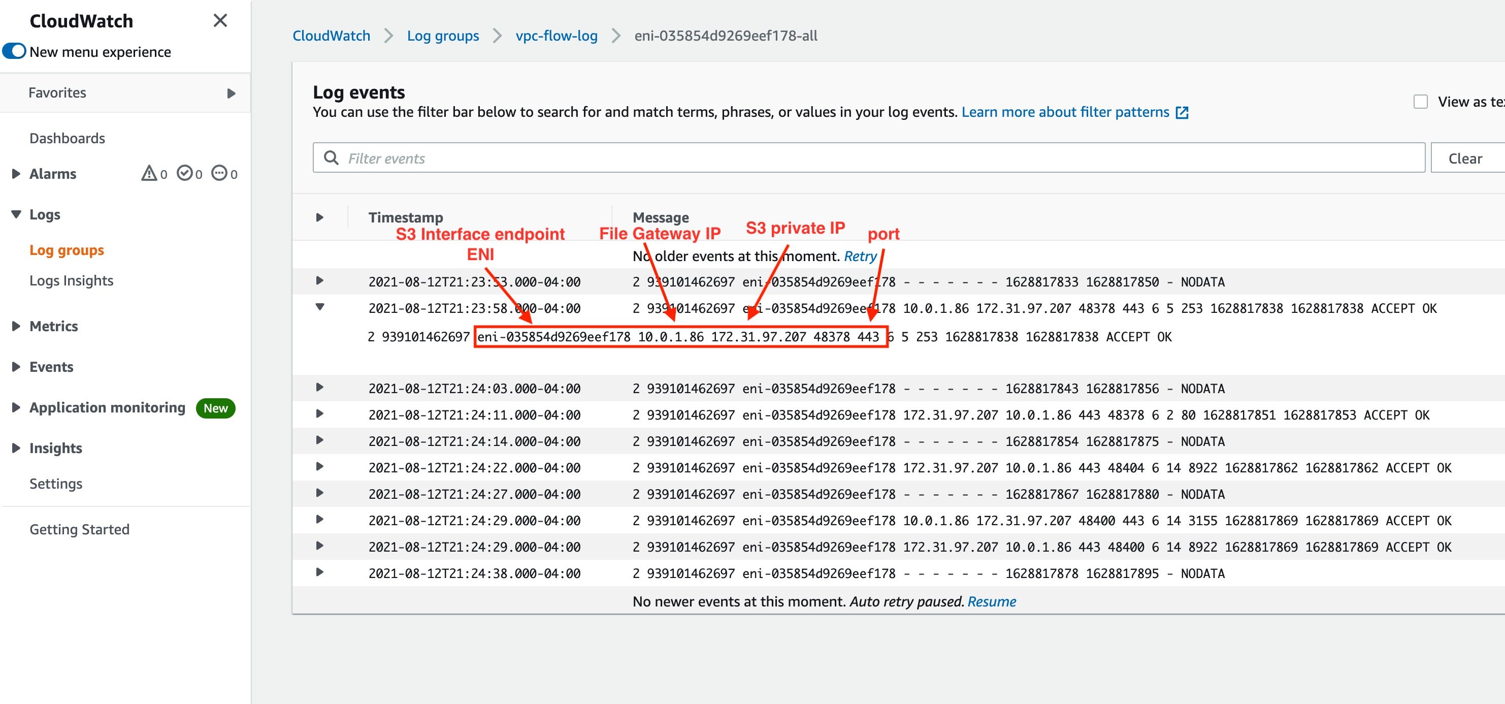
Figure 6. VPC Flow Log entry to verify connectivity using Private IPs
In this blog post, we have demonstrated how to use Amazon S3 File Gateway to transfer files to Amazon S3 buckets over AWS PrivateLink. Use this solution to securely copy your application data and files to cloud storage. This will also provide low latency access to that data from your on-premises applications.
Thanks for reading this blog post. If you have any feedback or questions, please add them in the comments section.
Further Reading:
Post Syndicated from Varun Rao Bhamidimarri original https://aws.amazon.com/blogs/big-data/authorize-sparksql-data-manipulation-on-amazon-emr-using-apache-ranger/
With Amazon EMR 5.32, Amazon EMR introduced Apache Ranger 2.0 support, which allows you to enable authorization and audit capabilities for Apache Spark, Amazon Simple Storage Service (Amazon S3), and Apache Hive. It also enabled authorization audits to be logged in Amazon CloudWatch. However, although you could control Apache Spark writes to Amazon S3 with these authorization capabilities, SparkSQL support was limited to only read authorization.
We’re happy to announce that with Amazon EMR 6.4, Apache Ranger SparkSQL integration supports authorizing capabilities for data manipulation statements (DML). You can now authorize INSERT INTO, INSERT OVERWRITE, and ALTER statements for SparkSQL using Apache Ranger policies.
Amazon EMR support for Apache SparkSQL is implemented using the Amazon EMR record server, which reads Apache Ranger policy definitions, evaluates access, and filters data before passing the data back to the individual Spark executors.
The following image shows the high-level architecture.
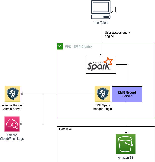
Before you begin, set up your Apache Ranger and EMR cluster. For instructions, see Introducing Amazon EMR integration with Apache Ranger. If you have an existing installation on Apache Ranger server with Apache Spark service definitions deployed, use the following code to redeploy the service definitions:
Now that the service definition has been updated, let’s test the policies.
For our use case, assume you have an external Amazon S3 backed partitioned Hive table. You want to use a SparkSQL DML statement to insert data into the table.
Use the following code for a table definition:
You can now set up the authorization policies on Apache Ranger. The following screenshots illustrate this process.
Because the table is externally backed by Amazon S3, we first need to enable read and write access to the Amazon S3 location of the table. If the location is on HDFS, the URL should have the HDFS path—for example, hdfs://xxxx.
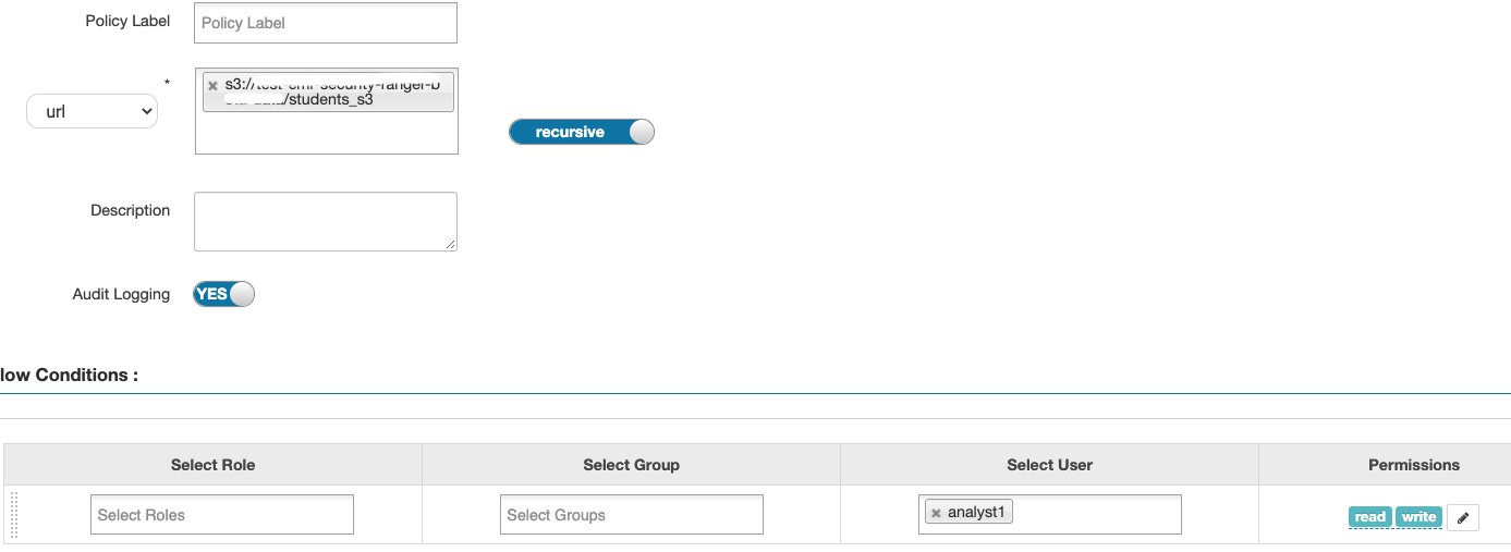
Next, we add SELECT, UPDATE, and ALTER permissions, allowing users to use the DML commands. Any update to the table metadata like statistics or partition information requires the ALTER permission.
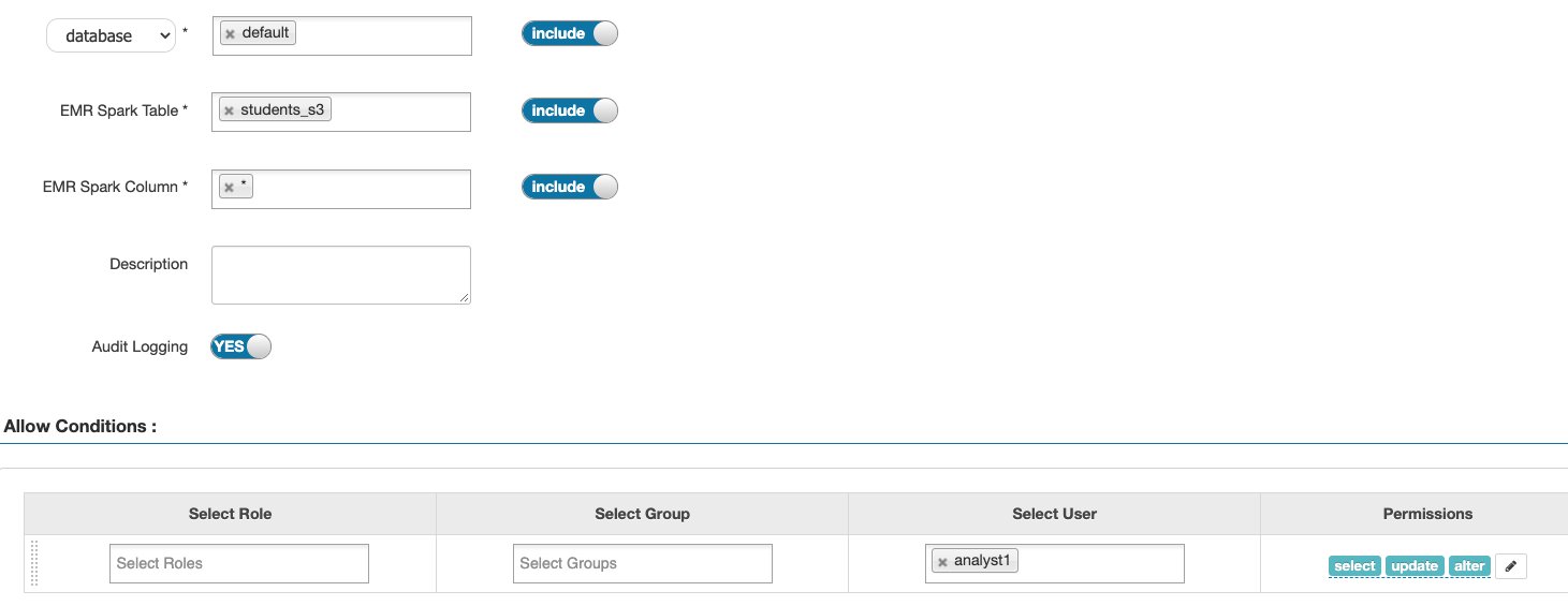
After we set up these Apache Ranger policies, we can start testing the DML statements. The following code is an example of an INSERT INTO statement:
The following screenshot shows our results.
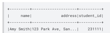
We can audit this action on CloudWatch, similar to other actions.


Inserting data into a partition where the partition location is different from the table location is not currently supported. The partition location must always be a child directory of the main table location.
| SQL statement/Ranger action | STATUS | Supported EMR release |
| SELECT | Supported | As of 5.32 |
| SHOW DATABASES | Supported | As of 5.32 |
| SHOW TABLES | Supported | As of 5.32 |
| SHOW COLUMNS | Supported | As of 5.32 |
| SHOW TABLE PROPERTIES | Supported | As of 5.32 |
| DESCRIBE TABLE | Supported | As of 5.32 |
| CREATE TABLE | Not Supported | |
| UPDATE TABLE | Not Supported | |
| INSERT OVERWRITE | Supported | As of 6.4 |
| INSERT INTO | Supported | As of 6.4 |
| ALTER TABLE | Supported | As of 6.4 |
| DELETE FROM | Not Supported |
Amazon EMR support for SparkSQL statements INSERT INTO, INSERT OVERWRITE, and ALTER TABLE with Apache Ranger is available on Amazon EMR 6.4 in the following AWS Regions:
For the latest Region availability, see the Amazon EMR Management Guide.
Amazon EMR 6.4 has introduced additional authorizing capabilities for data manipulation statements with Apache Ranger 2.0. You can use statements like INSERT INTO, INSERT OVERWRITE, and ALTER in SparkSQL and control authorization using Apache Ranger policies.
To additional information, see the following resources:
 Varun Rao Bhamidimarri is a Sr Manager, AWS Analytics Specialist Solutions Architect team. His focus is helping customers with adoption of cloud-enabled analytics solutions to meet their business requirements. Outside of work, he loves spending time with his wife and two kids, stay healthy, mediate and recently picked up gardening during the lockdown.
 Jalpan Randeri is a Senior Software Engineer at AWS. He likes working on performance optimization and data access controls for big data systems. Outside work, he likes watching anime & playing video games.