Post Syndicated from The History Guy: History Deserves to Be Remembered original https://www.youtube.com/watch?v=RJQeNoS3pRY
Giving back through Code Club | Meet Douglas
Post Syndicated from Sophie Ashford original https://www.raspberrypi.org/blog/giving-back-through-code-club-meet-douglas/
We love hearing from members of the community and sharing the stories of amazing young people, volunteers, and educators who are using their passion for technology to create positive change in the world around them.
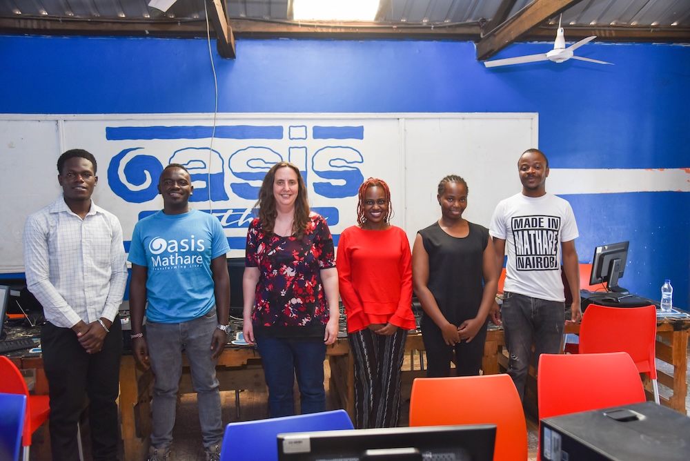
Growing up in Mathare, one of Nairobi’s largest informal settlements, Douglas experienced first-hand what it meant to go without access to education and opportunity. His experience sparked a Code Club journey that is already hugely inspiring… and it’s only just getting started.
Driven by a desire to help
For Douglas and many of his peers, the limited access to education in Mathare often meant being left with no clear path to earn a livelihood. Douglas saw opportunity in technology — he wanted to increase access in this field for the young people in Mathare and raise their ambitions.
“Why are we doing technology? Because we believe that tech does not have a boundary. As long as you have access to the internet and you can learn some basic skills… the opportunities are limitless.”
That belief became the keystone of Oasis Mathare, an organisation co-founded by Douglas and a group of others with similar lived experiences. Like Douglas, most of the founding members haven’t followed a standard path with formal schooling, but all understand the power of technology to transform lives.
From Photoshop to programming
Douglas’ own tech journey began humbly, and was sparked by his curiosity.
“After primary, I didn’t go straight to high school. I spent two years working in a nearby barber shop. Then I think I just fell in love with computers. I learned how to do some basic stuff with design and used to play around with Photoshop.”
From there, he taught himself web design and programming skills, which began to open new doors. Eventually, he went back to university to study business and information technology to deepen his knowledge, but even before that, Douglas had already started giving back.
“We used to hold a club providing a space for kids to come and play games on computers. That sort of grew from just Saturdays to a few times a week… and now it’s full time.”

Why Code Clubs?
Today, Oasis Mathare runs intensive software engineering and robotics programs that last between 9 and 12 months. But back in the early days of the organisation, Douglas quickly realised that many young people were struggling to keep up — not because of ability, but because they’d never used a computer before.
“So, we started Code Clubs to introduce these principles of programming at an early age… and we actually realised that those who have gone through Code Club take less time to complete our software engineering and robotics classes.”
Code Clubs now serve as a stepping stone at Oasis Mathare. They help introduce computer literacy and programming concepts to young people early, making it easier for them to thrive in more advanced programs.
The power of role models
The impact of the program is already visible. Many graduates of Oasis Mathare programs go on to volunteer and eventually teach, serving as role models for the younger learners.
“Oasis Mathare has 6 full-time staff. There are 12 Code Club leaders. They are our graduates from the software engineering program. We are plugging them into the Code Clubs to help them gain confidence and help the next generation.”
The Code Clubs are held both in schools and at the Oasis Mathare centre, creating safe, structured environments for learning, experimenting, and collaborating.

Building with what they have
Before setting up Code Clubs, Oasis Mathare ran STEM clubs that used a variety of resources, but the cost and maintenance became a barrier. When they discovered Code Club’s free-to-access resources, everything changed.
“We found [the resources] very useful. The good thing about Code Club is you can plan sessions using resources that are freely available, like Scratch. It’s really straightforward.”
The biggest challenge now? Internet access is limited, so Douglas and his team often work offline. The team have started using the Raspberry Pi Foundation’s offline resources, and look forward to more being available in the future.
What’s next for Douglas and Oasis Mathare?
Douglas and the Oasis Mathare team have already achieved so much. This was recognised with a royal seal of approval in 2018, when Douglas was honoured with the Queen’s Young Leaders Award by Queen Elizabeth at Buckingham Palace. Through the award, he gained access to world-class mentoring and leadership training from the University of Cambridge, helping him to amplify his impact back home.
So, what’s next? Douglas’ vision for the future is bold and clear.
“The main idea is to ensure that all kids in Mathare know at least one computer language. Not for the sake of it, but to use the principles of programming to solve their local problems.”
By learning coding, young people build more than just technical skills. They learn to think critically, work in teams, and solve problems in their communities. For Douglas, that’s the real impact.
“The overall goal is to ensure that no youth in Mathare are left behind and they all have the opportunity to develop essential skills from an early age.”

Looking further ahead
Oasis Mathare runs Code Clubs weekly, all year round, and Douglas is always looking for ways to expand the program’s reach, especially through partnerships, sponsorships, and sharing their successes so far.
With more resources, more local leaders, and a whole community behind him, Douglas is rewriting the narrative for young people in Mathare. You can find out more about Oasis Mathare on their official website.
If you’d like to support young people in your community to explore coding, why not start a Code Club? The team will support you every step of the way with resources, training, and a collaborative community. Find out more on the Code Club website.
The post Giving back through Code Club | Meet Douglas appeared first on Raspberry Pi Foundation.
Watch out Leica – SONY Are coming for you! Sony RX1R III PREMIUM Compact Camera 📷
Post Syndicated from Matt Granger original https://www.youtube.com/watch?v=jAqu4vlwqa4
Comic for 2025.07.16 – Inspiration
Post Syndicated from Explosm.net original https://explosm.net/comics/inspiration
New Cyanide and Happiness Comic
Compaction support for Avro and ORC file formats in Apache Iceberg tables in Amazon S3
Post Syndicated from Angel Conde Manjon original https://aws.amazon.com/blogs/big-data/compaction-support-for-avro-and-orc-file-formats-in-apache-iceberg-tables-in-amazon-s3/
Apache Iceberg, a high-performance open table format (OTF), has gained widespread adoption among organizations managing large scale analytic tables and data volumes. Iceberg brings the reliability and simplicity of SQL tables to data lakes while enabling engines like Apache Spark, Apache Trino, Apache Flink, Apache Presto, Apache Hive, Apache Impala, and AWS analytic services like Amazon Athena to flexibly and securely access data with lakehouse architecture. While the lakehouse built using Iceberg represents an evolution to the data lake, but it still requires services to compact and optimize the files and partitions that comprise the tables. Self-managing Iceberg tables with large volumes of data poses several challenges, including managing concurrent transactions, processing real-time data streams, handling small file proliferation, maintaining data quality and governance, and ensuring compliance.
At re:Invent 2024, Amazon S3 introduced Amazon S3 Tables marking the first cloud object store with native Iceberg support for Parquet files, designed to streamline tabular data management at scale. Parquet is one of the most common and fastest growing data types in Amazon S3. Amazon S3 stores exabytes of Parquet data, and averages over 15 million requests per second to this data. While S3 Tables initially supported Parquet file type, as discussed in the S3 Tables AWS News Blog, the Iceberg specification extends to Avro, and ORC file formats for managing large analytic tables. Now, S3 Tables is expanding its capabilities to include automatic compaction for these additional file types within Iceberg tables. This enhancement is also available for Iceberg tables on general purpose S3 buckets, using the lakehouse architecture of Amazon SageMaker that previously supported Parquet compaction as covered in the blog post Accelerate queries on Apache Iceberg tables through AWS Glue auto compaction.
This blog post explores the performance benefits of automatic compaction of Iceberg tables using Avro and ORC file types in S3 Tables for a data ingestion use with over 20 billion events.
Parquet, ORC, and Avro file formats
Parquet is one of the most common and fastest growing data types in Amazon S3. It was originally developed by Twitter and now part of the Apache ecosystem, is known for its broad compatibility with big data tools such as Spark, Hive, Impala, and Drill. Amazon S3 stores exabytes of Apache Parquet data, and averages over 15 million requests per second to this data. Parquet uses a hybrid encoding scheme and supports complex nested data structures, making it ideal for read-heavy workloads and analytics across various platforms. Parquet also provides excellent compression and efficient I/O by enabling selective column reads, reducing the amount of data scanned during queries.
ORC was specifically designed for Hadoop ecosystem and optimized for Hive. It generally offers better compression ratios and better read performance for certain types of queries due to its lightweight indexing and aggressive predicate pushdown capabilities. ORC includes built-in statistics and supports lightweight indexes, which can accelerate filtering operations significantly. While Parquet offers broader tool compatibility, ORC often outperforms it within Hive-centric environments, especially when dealing with flat data structures and large sequential scans.
Avro file format is usually used in streaming scenarios for its serialization and schema handling capabilities and for its seamless integration with Apache Kafka, offering a powerful combination for handling real-time data streams. For example, for storing and validating streaming data schemas, you have the option of using AWS Glue Schema registry in AWS. Avro, in contrast with Parquet and ORC, is a row-based storage format designed for efficient data serialization and schema evolution. Avro excels in write-heavy use cases like data ingestion and streaming and is commonly used with Kafka. Unlike Parquet and ORC, which are optimized for analytical queries, Avro is designed for fast reads and writes of complete records, and it stores the schema alongside the data, enabling easier data exchange and evolution over time.
Below is a comparison of these 3 file formats.
| Parquet | ORC | Avro | |
| Storage format | Columnar | Columnar | Row-based |
| Best for | Analytics & queries across columns | Hive-based queries, heavy compression | Data ingestion, streaming, serialization |
| Compression | Good | Excellent (especially numerical data) | Moderate |
| Tool compatibility | Broad (Spark, Hive, Presto, etc.) | Strong with Hive/Hadoop | Strong with Kafka, Flink, etc. |
| Query performance | Very good for analytics | Excellent in Hive | Not optimized for analytics |
| Schema evolution | Supported | Supported | Excellent (schema stored with data) |
| Nested data support | Yes | Limited | Yes |
| Write efficiency | Moderate | Moderate | High |
| Read efficiency | High (for columnar scans) | Very high (in Hive) | High (for full record reads) |
Solution Overview
We run two versions of the same architecture: one where the tables are auto compacted, and another without compaction using in this case S3 Tables. By comparing both scenarios, this post demonstrates the efficiency, query performance, and cost benefits of auto compacted tables vs. non-compacted tables in a simulated Internet of Things (IoT) data pipeline. The following diagram illustrates the solution architecture.
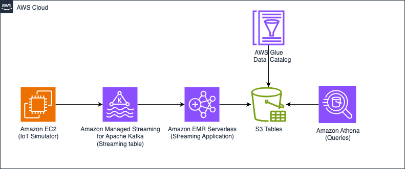
Figure 1 – Solution architecture diagram
Compaction performance test
We simulated IoT data ingestion with over 20 billion events and used MERGE INTO for data deduplication across two time-based partitions, involving heavy partition reads and shuffling. After ingestion, we ran queries in Athena to compare performance between compacted and uncompacted tables using the Merge on Read (MoR) mode on both Avro and ORC formats. We use the following table configuration settings:
We use 'write.distribution.mode=hash' to generate bigger files that will benefit the performance. Note that as we are generating quite large files already the differences between un-compacted and compacted tables are not going to that big, this will change significantly depending on your workload (for example, partitioning, input rate, batch size) and your chosen write distribution mode. For more details, please refer to the Writing Distribution Modes section in the Apache Iceberg documentation.
The following table shows metrics of the Athena query performance. Please refer to section “Query and Join data from these S3 Tables to build insights” for query details. All table sizes used to analyze the query performance are over 2 billion rows. These results are specific to this simulation exercise and the readers’ results may vary depending on their data size and queries they are running.
| Query | Avro query time compaction | Avro query time without compaction | ORC query time without compaction | ORC query time with compaction | % improvement Avro | % improvement ORC |
| Query 1 | 22.45 secs | 26.54 secs | 30.16 secs | 20.32 secs | 15.41% | 32.63% |
| Query 2 | 22.68 secs | 25.83 secs | 34.17 secs | 20.51 secs | 12.20% | 39.98% |
| Query 3 | 25.92 secs | 35.65 secs | 29.05 secs | 24.95 secs | 27.29% | 14.11% |
Prerequisites
To set up your own evaluation environment and test the feature, you need the following prerequisites.
AWS account with access to the following AWS services:
- Amazon S3 including S3 Tables.
- AWS Lake Formation and AWS Glue Data Catalog.
- AWS Glue.
- A virtual private cloud (VPC) with at least two private subnets. For instructions, see Create a VPC.
- An EC2 instance c5.xlarge using Amazon Linux 2023 running on one of those private subnets where you will launch the data simulator. For the security group, you can use the default for the VPC. For more information, see Get started with Amazon EC2.
- An AWS Identity and Access Management (IAM) user with the correct permissions to create and configure all the required resources.
Create S3 table bucket and enable integration with AWS analytics services
Go to S3 console and enable table buckets feature.
Then choose the Create table bucket button, fill Table bucket name with any bucket name you prefer, select the Enable integration checkbox, then choose Create table bucket.
Set up Amazon S3 storage
Create an S3 bucket with the following structure:
Download the descriptor file employee.desc from the GitHub repo and put it into the S3 bucket you just created.
Download the application on the releases page
Get the packaged application S3Tables-Avro-orc-auto-compaction-benchmark-0.1 from the GitHub repo, then upload the JAR file to the “jars” directory on the S3 bucket. Checkpoint will be used for the Structured Streaming checkpointing mechanism. Because we use 4 streaming job runs, one for compacted and one for uncompacted data on each format, we also create a “checkpointAuto” folder for both.
Create an EMR Serverless application
Create an EMR Serverless application with the following settings (for instructions, see Getting started with Amazon EMR Serverless):
- Type: Spark
- Version: 7.20
- Architecture: x86_64
- Java Runtime: Java 17
- Metastore Integration: AWS Glue Data Catalog
- Logs: Enable Amazon CloudWatch Logs if desired (it’s recommended but not required for this blog)
Configure the network (VPC, subnets, and default security group) to allow the EMR Serverless application to reach the MSK cluster. Take note of the application-id to use later for launching the jobs.
Create an MSK cluster
Create an MSK cluster on the Amazon MSK console. For more details, see Get started using Amazon MSK. You need to use custom create with at least two brokers using 3.5.1, Apache Zookeeper mode version, and instance type kafka.m7g.xlarge. Do not use public access, instead choose two private subnets to deploy (one broker per subnet or Availability Zone, for a total of two brokers). For the security group, remember that the EMR cluster and the Amazon EC2 based producer will need to reach the cluster and act accordingly.
For security, use PLAINTEXT (in production, you should secure access to the cluster). Choose 200 GB as storage size for each broker and do not enable tiered storage. For network security groups, you can choose the default of the VPC.
For the MSK cluster configuration, use the following settings:
Configure the data simulator
Log in to your EC2 instance. Because it’s running on a private subnet, you can use an instance endpoint to connect. To create one, see Connect to your instances using EC2 Instance Connect Endpoint. After you log in, issue the following commands:
Create Kafka topics
Create two Kafka topics—remember that you need to change the bootstrap server with the corresponding client information. You can get this data from the Amazon MSK console on the details page for your MSK cluster.
Launching EMR Serverless Jobs for Iceberg Tables (Avro/ORC – Compacted & Non-Compacted)
Now it is time to launch EMR Serverless streaming jobs for four different Iceberg tables. Each job uses a different Spark Structured Streaming checkpoint and a specific Java class for ingestion logic.
Before launching the jobs, make sure:
- You have disabled auto-compaction in the S3 tables where necessary (see S3 Tables maintenance). In this case for
employee_Avro_uncompactedandemployee_orc_uncompactedtables. - Your EMR Serverless IAM role has permissions to read/write from S3Tables. Open AWS Lake formation console, then, you can follow these docs to give permissions to the EMR Serverless Role.
After launching each job launch the data simulator and let it finish. Then you can cancel the job run and launch the next one ( while launching the data simulator again).
Launch the data simulator
Download the JAR file to the EC2 instance and run the producer, note that will do this once.
aws s3 cp s3://s3bucket/jars/streaming-iceberg-ingest-1.0-SNAPSHOT.jar .
Now you can start the protocol buffer producers. Use the following commands:
You should run this command for each of the tables ( job runs), run the command after the ingestion process has started.
Table 1: employee_orc_uncompacted
Checkpoint: checkpointORC
Java Class: SparkCustomIcebergIngestMoRS3BucketsORC
Table 2: employee_avro_uncompacted
Checkpoint: checkpointAvro
Java Class: SparkCustomIcebergIngestMoRS3BucketsAvro
Table 3: employee_orc (Auto-Compacted)
Checkpoint: checkpointORCAuto
Java Class: SparkCustomIcebergIngestMoRS3BucketsAutoORC
Table 4: employee_avro (Auto-Compacted)
Checkpoint: checkpointAvroAuto
Java Class: SparkCustomIcebergIngestMoRS3BucketsAutoAvro
Query and Join data from these S3 Tables to build insights
You can go to Athena console and then run the queries. Please ensure that Lake Formation permissions are applied on the catalog database and tables for your IAM Console role. For more details, please refer to docs on the Grant Lake Formation permissions on your table.
To benchmark these queries in Athena, you can run each query multiple times—typically five runs per query—to obtain a reliable performance estimate. In the Athena console, simply execute the same query repeatedly and record the execution time for each run, which is displayed in the query history. Once you have five execution times, calculate the average to get a representative benchmark value. This approach helps account for variations in performance due to background load, providing more consistent and meaningful results.
Query 1
Query 2
Query 3
Conclusion
AWS has expanded support for Iceberg table optimization to include all Iceberg supported file formats: Parquet, Avro, and ORC. This comprehensive compaction capability is now available for both Amazon S3 Tables and Iceberg tables in general purpose S3 buckets using the lakehouse architecture in SageMaker with Glue Data Catalog optimization. S3 Tables deliver a fully managed experience through continual optimization, automatically maintaining your tables by handling compaction, snapshot retention, and unreferenced file removal. These automated maintenance features significantly improve query performance and reduce query engine costs. Compaction support for Avro and ORC formats is now available in all AWS Regions where S3 Tables or optimization with the AWS Glue Data Catalog are available. To learn more about S3 Tables compaction, see the S3 Tables maintenance documentation. For general purpose bucket optimization, see the Glue Data Catalog optimization documentation.
Special thanks to everyone who contributed to this launch: Matthieu Dufour, Srishti Bhargava, Stylianos Herodotou, Kannan Ratnasingham, Shyam Rathi, David Lee.
About the authors
 Angel Conde Manjon is a Sr. EMEA Data & AI PSA, based in Madrid. He has previously worked on research related to Data Analytics and Artificial Intelligence in diverse European research projects. In his current role, Angel helps partners develop businesses centered on Data and AI.
 Diego Colombatto is a Principal Partner Solutions Architect at AWS. He brings more than 15 years of experience in designing and delivering Digital Transformation projects for enterprises. At AWS, Diego works with partners and customers advising how to leverage AWS technologies to translate business needs into solutions. Solution architectures, algorithmic trading and cooking are some of his passions and he’s always open to start a conversation on these topics.
 Sandeep Adwankar is a Senior Technical Product Manager at AWS. Based in the California Bay Area, he works with customers around the globe to translate business and technical requirements into products that enable customers to improve how they manage, secure, and access data.
A Stone Slab of Rare Value
Post Syndicated from The History Guy: History Deserves to Be Remembered original https://www.youtube.com/shorts/gbHFr60NlgU
Grab’s service mesh evolution: From Consul to Istio
Post Syndicated from Grab Tech original https://engineering.grab.com/service-mesh-evolution
The challenge: When good enough isn’t good enough
Picture this: It’s 2024, and Grab’s microservices ecosystem is thriving with over 1000 services running in different infrastructure. But behind the scenes, our service mesh setup is showing its age. We’re running Consul with a fallback mechanism called Catcher – a setup that has served us well but is starting to feel like wearing a winter coat in Singapore’s heat.
The challenges we faced were becoming increasingly apparent. A single Consul server issue could trigger a fleet-wide impact, affecting critical services like food delivery and ride-hailing. Our fallback solution, while necessary, added complexity and limited our ability to implement advanced features like circuit breaking and retry policies. As we expanded our presence across Southeast Asia, the need for robust multi-cluster support became more critical than ever. The existing setup struggled with modern requirements like advanced traffic management and fine-grained security controls, while the growing complexity of our microservices architecture demanded better traffic management capabilities.
The complexity of Grab’s infrastructure
Our infrastructure landscape is as diverse as the Southeast Asian markets we serve. We operate a complex hybrid environment encompassing services on traditional VMs and EKS clusters with diverse infrastructure provisioning and deployment approaches. This diversity isn’t merely about deployment models—it’s about meeting the unique needs of different business units and regulatory requirements across the region.
The complexity doesn’t stop there. We handle dual traffic protocols (HTTP and gRPC) across our entire service ecosystem. Our services communicate across cloud providers between AWS and GCP. Within AWS alone, we maintain multiple organizations to segregate different Grab entities, each operating in its own isolated network. This multi-cloud, multi-protocol, multi-organization setup presented unique challenges for our service mesh implementation.
The quest for a better solution
Like any good tech team, we didn’t just jump to conclusions. We embarked on a thorough evaluation of service mesh solutions, considering various options including Application Load Balancer (ALB), Istio, AWS Lattice, and Linkerd. Our evaluation process was comprehensive and focused on real-world needs, examining everything from stability under high load to the performance impact on service-to-service communication.
We needed a solution that could handle our distributed architecture while maintaining operational simplicity. The ideal service mesh would need to integrate seamlessly with our existing infrastructure landscape while offering the flexibility to scale with our growing needs. After careful consideration, Istio emerged as the clear winner, offering robust multi-cluster support with flexible deployment models and a comprehensive set of features for traffic management, security, and observability.
What really sealed the deal was Istio’s strong Kubernetes integration and native support, combined with active community backing. The rich ecosystem of tools and integrations meant we wouldn’t be building everything from scratch, while the flexible deployment options could accommodate our unique requirements.
Designing our Istio architecture
When it came to designing our Istio implementation, we took a slightly unconventional approach. Instead of following the traditional “one control plane per cluster” pattern, we designed a more resilient architecture that would better suit our needs. We implemented multiple control planes running on dedicated Kubernetes clusters for better isolation and scalability, with active-active pairs ensuring high availability.
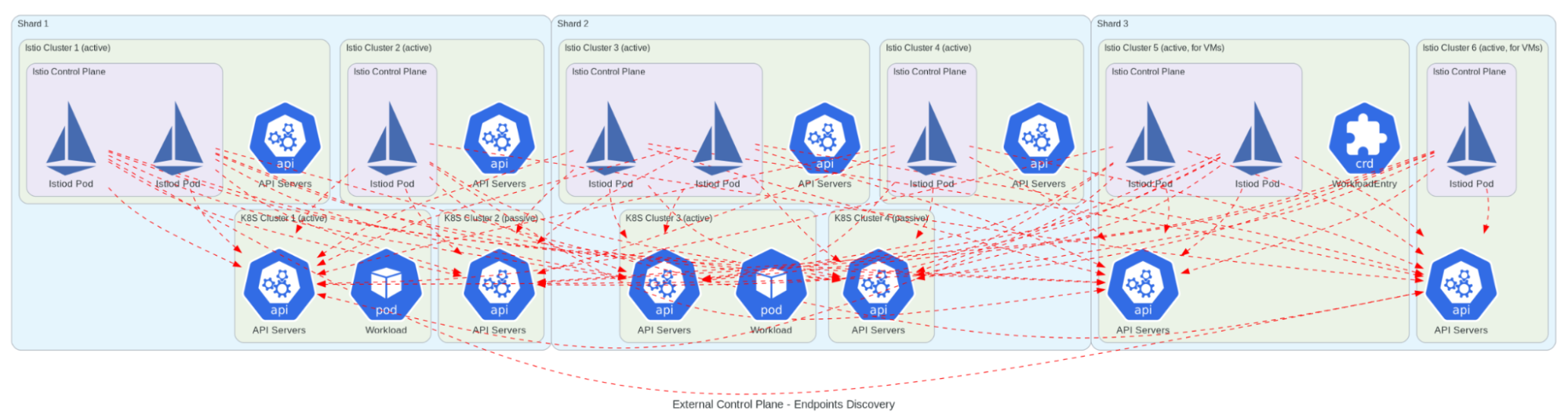
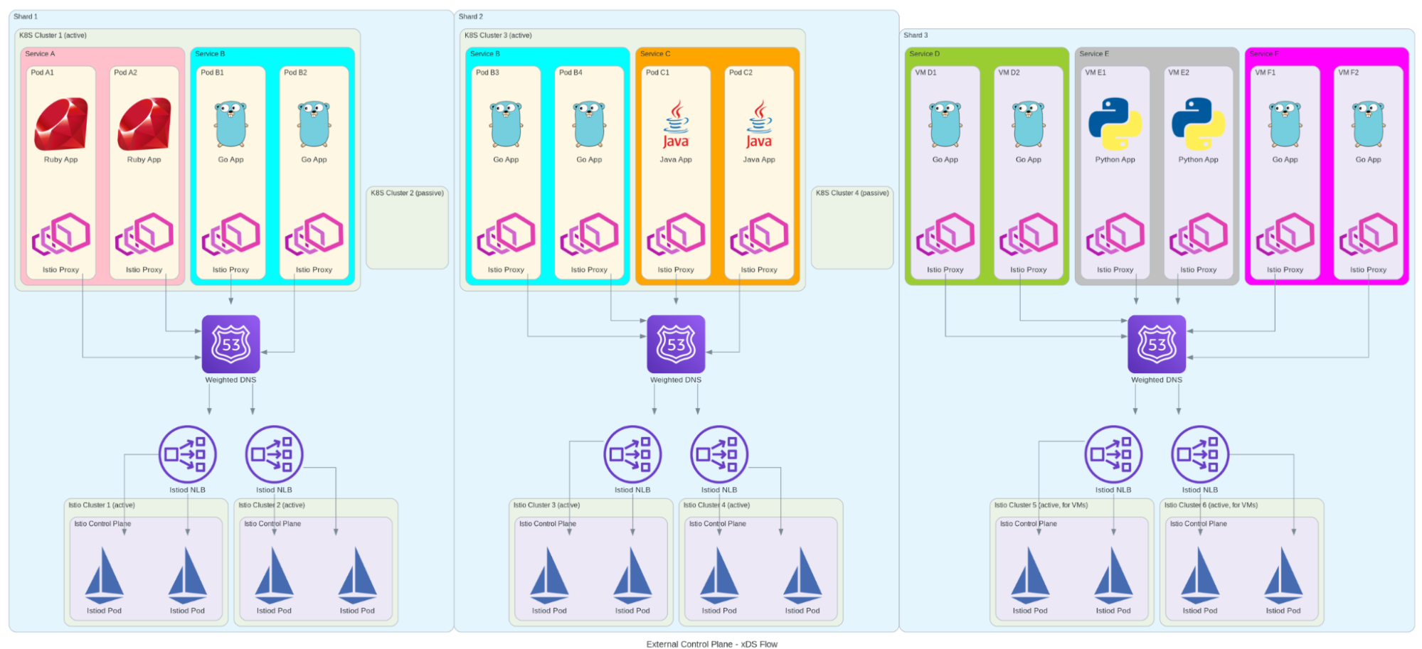
Our architecture needed to support high-throughput service-to-service communication while enabling complex routing rules for A/B testing and canary deployments. We implemented custom resource definitions for service mesh configuration and integrated with our existing monitoring and alerting systems. The organization-based mesh boundaries we designed would support our multi-tenant architecture, while our solution for cross-cluster endpoint discovery would ensure reliable service communication across our distributed system.
This design wasn’t just about following best practices – it was about learning from our past experiences with etcd and Consul. We wanted a setup that could handle Grab’s scale while maintaining simplicity and reliability. The architecture needed to support everything from high-throughput service-to-service communication to complex routing rules for A/B testing and canary deployments, all while maintaining fine-grained security policies and comprehensive observability.
The migration journey begins
In Q4 2024, we kicked off our migration journey with a clear plan. While our initial strategy focused on gRPC traffic migration, real-world priorities led us down a different path. Our first major milestone was the GCP to AWS migration, a cross-cloud initiative that would test our service mesh capabilities in a complex, multi-cloud environment.
This cross-cloud migration was a significant undertaking, requiring careful coordination between teams and careful consideration of network policies, security requirements, and service dependencies. We had to ensure seamless communication between services running in different cloud providers while maintaining security and performance standards.
Alongside our ongoing cloud migration efforts, we launched parallel initiatives focused on gRPC and HTTP traffic migration with cross-mesh connectivity requirements. This phase introduced distinct challenges, as it involved migrating business-critical services while implementing gradual traffic shifting capabilities and quick rollback mechanisms to ensure zero-downtime migrations. We also maintained close monitoring of performance metrics throughout the process.
Additionally, we needed to ensure seamless compatibility between different service mesh implementations and navigate the complexities of cross-mesh communication. The insights and experience gained from our cloud migration phase have proven invaluable in informing our approach and execution strategy for this critical migration effort.
The journey hasn’t been without its challenges. We’ve had to balance migration speed with stability while coordinating across multiple teams and organizations. Handling both gRPC and HTTP traffic patterns required careful planning and execution. We’ve had to deal with legacy systems and technical debt while training and supporting teams through the transition. Maintaining service continuity during these transitions has been our top priority.
Lessons learned
This journey has taught us several valuable lessons. We’ve learned that sometimes the standard approach isn’t the best fit, and innovation often comes from questioning assumptions. We’ve discovered the importance of balancing innovation with stability, taking calculated risks while building capability for a quick mitigation.
Keeping the bigger picture in mind has been crucial, considering long-term implications and planning for scale and growth. We’ve learned to document challenges and solutions, sharing knowledge across teams to avoid repeating mistakes. Most importantly, we’ve learned to stay flexible and adapt to changing needs, being ready to pivot when necessary while keeping an eye on emerging technologies.
What’s next?
The service mesh landscape is constantly evolving, and we’re excited to be part of this journey. Our next steps include continuing our migration efforts with a focus on stability while exploring mesh features like advanced traffic management, and enhanced security policies.
We’re also working on enhancing our operational capabilities through automated testing and validation, improved monitoring and alerting, and better debugging tools. As we progress, we’re committed to sharing our experiences with the community through open source contributions, conference participation, and technical blogs.
Shape the future with us
We’re not just implementing a service mesh—we’re architecting the backbone of Grab’s microservices future. Every decision prioritizes reliability, scalability, and maintainability, ensuring we build something that will stand the test of time.
The journey continues, and we’re excited about what lies ahead. Follow our progress for real-world insights that might shape your own service mesh evolution.
Want to help us build the future? We have exciting opportunities waiting for you.
Credits to the Service Mesh team: Aashif Bari, Hilman Kurniawan, Hofid Mashudi, Jingshan Pang, Kaitong Guo, Mikko Turpeinen, Sok Ann Yap, Jesse Nguyen, and Xing Yii.
Join us
Grab is a leading superapp in Southeast Asia, operating across the deliveries, mobility and digital financial services sectors. Serving over 800 cities in eight Southeast Asian countries, Grab enables millions of people everyday to order food or groceries, send packages, hail a ride or taxi, pay for online purchases or access services such as lending and insurance, all through a single app. Grab was founded in 2012 with the mission to drive Southeast Asia forward by creating economic empowerment for everyone. Grab strives to serve a triple bottom line – we aim to simultaneously deliver financial performance for our shareholders and have a positive social impact, which includes economic empowerment for millions of people in the region, while mitigating our environmental footprint.
Powered by technology and driven by heart, our mission is to drive Southeast Asia forward by creating economic empowerment for everyone. If this mission speaks to you, join our team today!
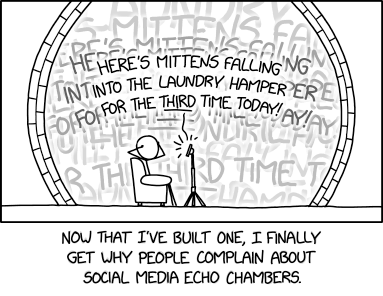
Echo Chamber
Post Syndicated from xkcd.com original https://xkcd.com/3116/
Streamline the path from data to insights with new Amazon SageMaker Catalog capabilities
Post Syndicated from Donnie Prakoso original https://aws.amazon.com/blogs/aws/streamline-the-path-from-data-to-insights-with-new-amazon-sagemaker-capabilities/
Modern organizations manage data across multiple disconnected systems—structured databases, unstructured files, and separate visualization tools—creating barriers that slow analytics workflows and limit insight generation. Separate visualization platforms often create barriers that prevent teams from extracting comprehensive business insights.
These disconnected workflows prevent your organizations from maximizing your data investments, creating delays in decision making and missed opportunities for comprehensive analysis that combines multiple data types.
Starting today, you can use three new capabilities in Amazon SageMaker to accelerate your path from raw data to actionable insights:
- Amazon QuickSight integration – Launch Amazon QuickSight directly from Amazon SageMaker Unified Studio to build dashboards using your project data, then publish them to the Amazon SageMaker Catalog for broader discovery and sharing across your organization.
- Amazon SageMaker adds support for Amazon S3 general purpose buckets and Amazon S3 Access Grants in SageMaker Catalog– Make data stored in Amazon S3 general purpose buckets easier for teams to find, access, and collaborate on all types of data including unstructured data, while maintaining fine-grained access control using Amazon S3 Access Grants.
- Automatic data onboarding from your lakehouse – Automatic onboarding of existing AWS Glue Data Catalog (GDC) datasets from the lakehouse architecture into SageMaker Catalog, without manual setup.
These new SageMaker capabilities address the complete data lifecycle within a unified and governed experience. You get automatic onboarding of existing structured data from your lakehouse, seamless cataloging of unstructured data content in Amazon S3, and streamlined visualization through QuickSight—all with consistent governance and access controls.
Let’s take a closer look at each capability.
Amazon SageMaker and Amazon QuickSight Integration
With this integration, you can build dashboards in Amazon QuickSight using data from your Amazon SageMaker projects. When you launch QuickSight from Amazon SageMaker Unified Studio, Amazon SageMaker automatically creates the QuickSight dataset and organizes it in a secured folder accessible only to project members.
Furthermore, the dashboards you build stay within this folder and automatically appear as assets in your SageMaker project, where you can publish them to the SageMaker Catalog and share them with users or groups in your corporate directory. This keeps your dashboards organized, discoverable, and governed within SageMaker Unified Studio.
To use this integration, both your Amazon SageMaker Unified Studio domain and QuickSight account must be integrated with AWS IAM Identity Center using the same IAM Identity Center instance. Additionally, your QuickSight account must exist in the same AWS account where you want to enable the QuickSight blueprint. You can learn more about the prerequisites on Documentation page.
After these prerequisites are met, you can enable the blueprint for Amazon QuickSight by navigating to the Amazon SageMaker console and choosing the Blueprints tab. Then find Amazon QuickSight and follow the instructions.

You also need to configure your SQL analytics project profile to include Amazon QuickSight in Add blueprint deployment settings.
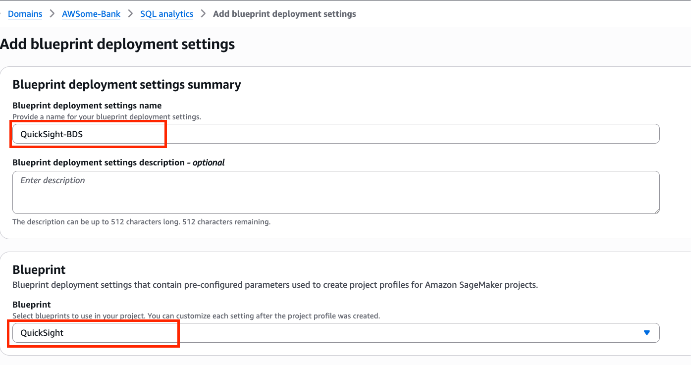
To learn more on onboarding setup, refer to the Documentation page.
Then, when you create a new project, you need to use the SQL analytics profile.
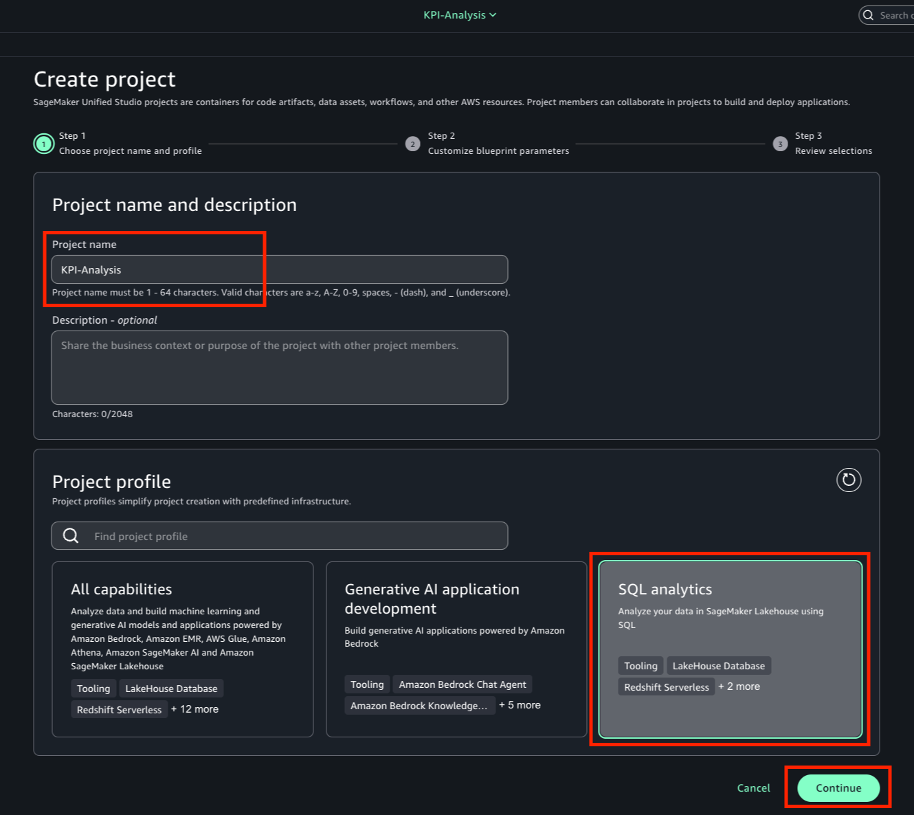
With your project created, you can start building visualizations with QuickSight. You can navigate to the Data tab, select the table or view to visualize, and choose Open in QuickSight under Actions.
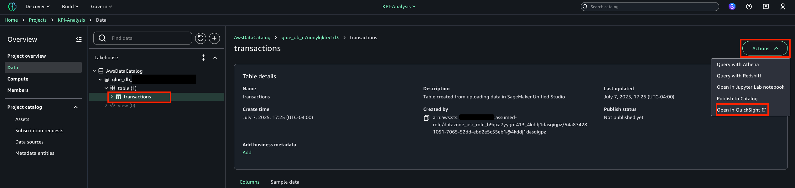
This will redirect you to the Amazon QuickSight transactions dataset page and you can choose USE IN ANALYSIS to begin exploring the data.
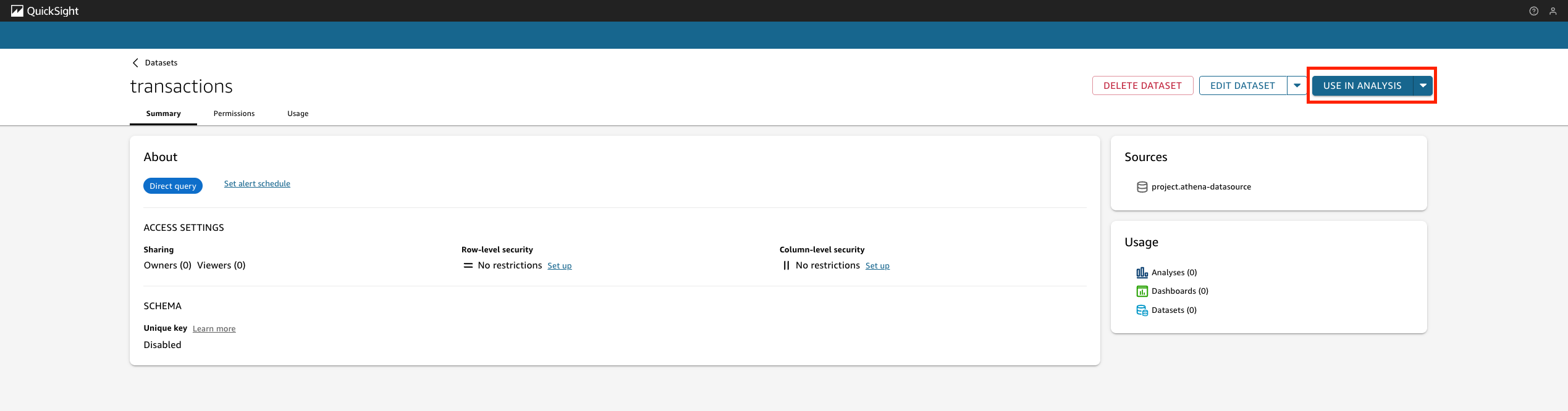
When you create a project with the QuickSight blueprint, SageMaker Unified Studio automatically provisions a restricted QuickSight folder per project where SageMaker scopes all new assets—analyses, datasets, and dashboards. The integration maintains real-time folder permission sync, keeping QuickSight folder access permissions aligned with project membership.
Amazon Simple Storage Service (S3) general purpose buckets integration
Starting today, SageMaker adds support for S3 general purpose buckets in SageMaker Catalog to increase discoverability and allows granular permissions through S3 Access Grants, enabling users to govern data, including sharing and managing permissions. Data consumers, such as data scientists, engineers, and business analysts, can now discover and access S3 assets through SageMaker Catalog. This expansion also enables data producers to govern security controls on any S3 data asset through a single interface.
To use this integration, you need appropriate S3 general purpose bucket permissions, and your SageMaker Unified Studio projects must have access to the S3 buckets containing your data. Learn more about prerequisites on Amazon S3 data in Amazon SageMaker Unified Studio Documentation page.
You can add a connection to an existing S3 bucket.
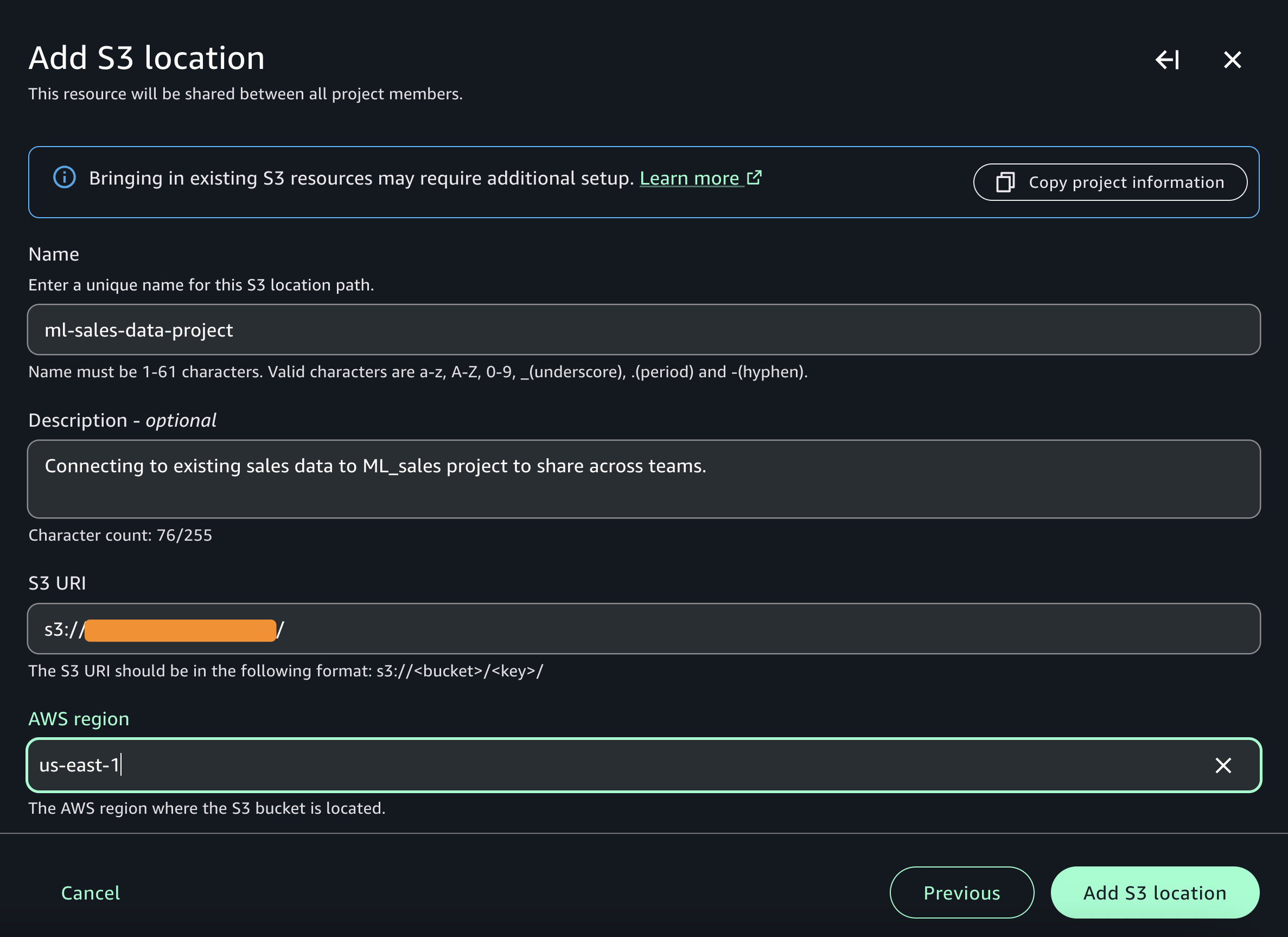
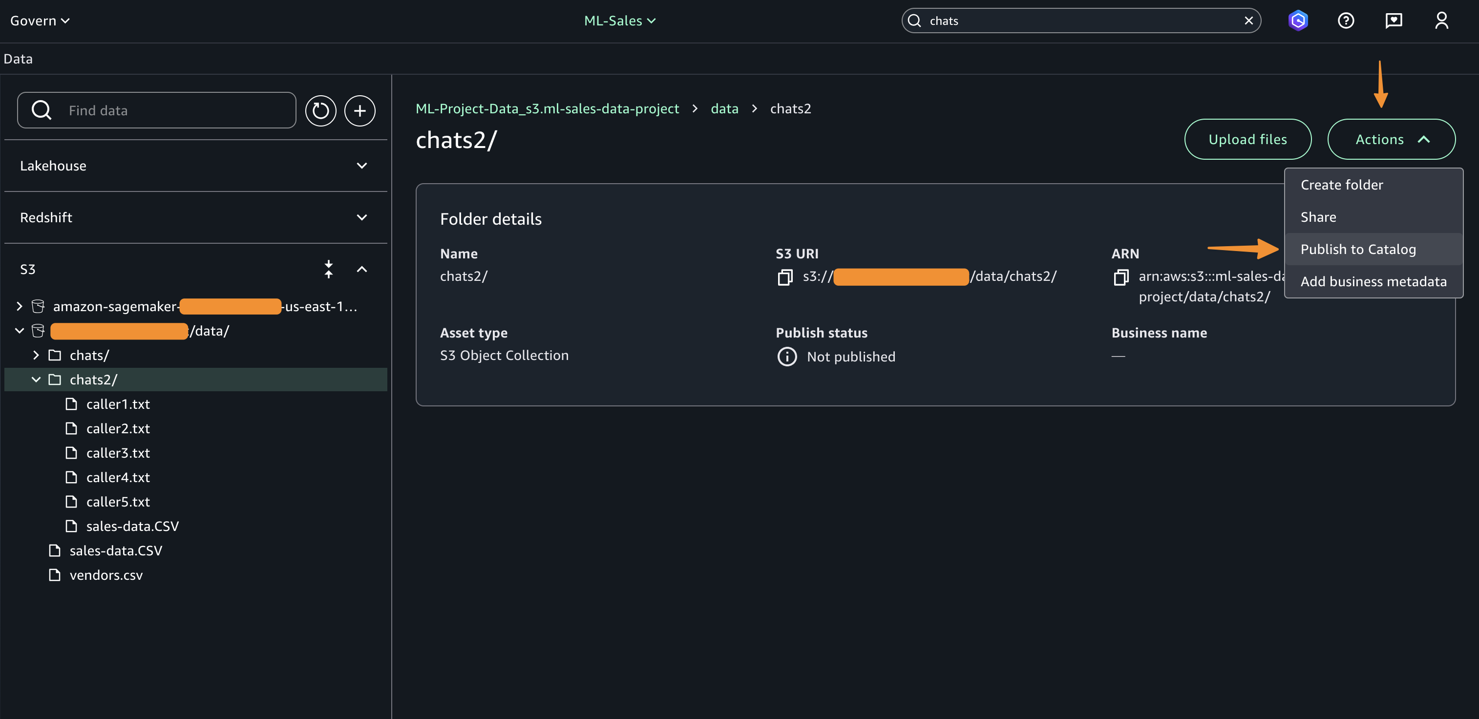
When it’s connected, you can browse accessible folders and create discoverable assets by choosing on the bucket or a folder and selecting Publish to Catalog.
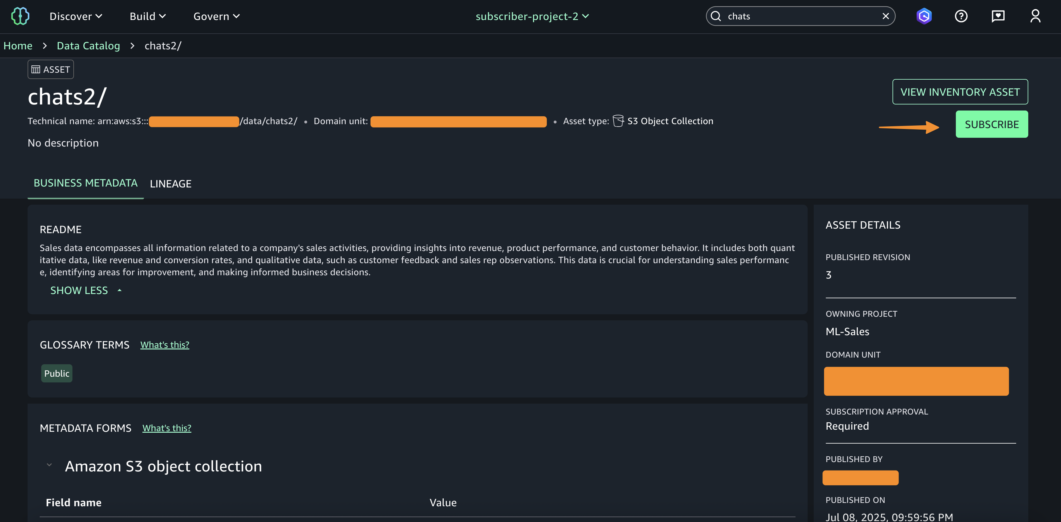
This action creates a SageMaker Catalog asset of type “S3 Object Collection” and opens an asset details page where users can augment business context to improve search and discoverability. Once published, data consumers can discover and subscribe to these cataloged assets. When data consumers subscribe to “S3 Object Collection” assets, SageMaker Catalog automatically grants access using S3 Access Grants upon approval, enabling cross-team collaboration while ensuring only the right users have the right access.
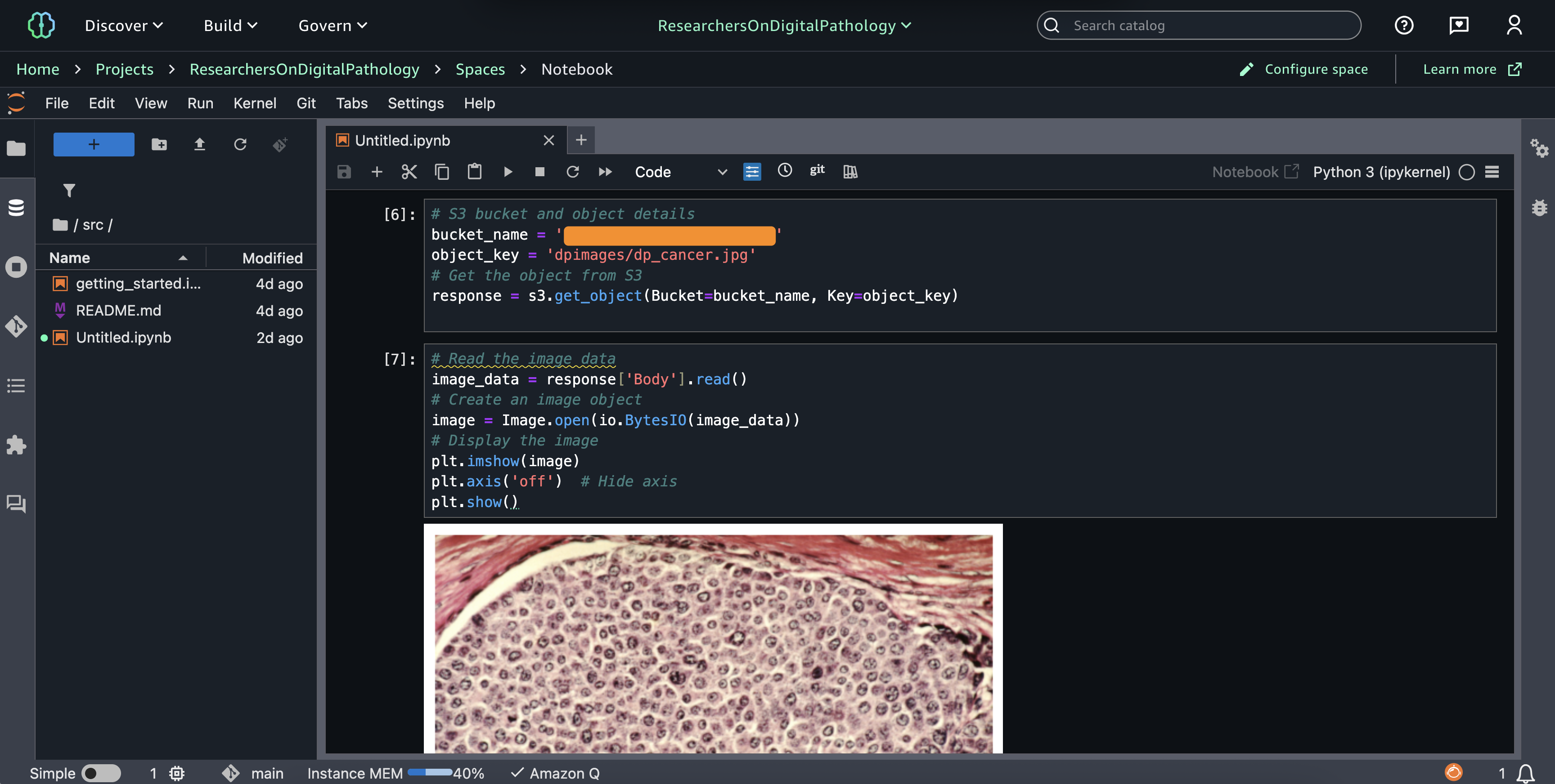
When you have access, now you can process your unstructured data in Amazon SageMaker Jupyter notebook. Following screenshot is an example to process image in medical use case.
If you have structured data, you can query your data using Amazon Athena or process using Spark in notebooks.
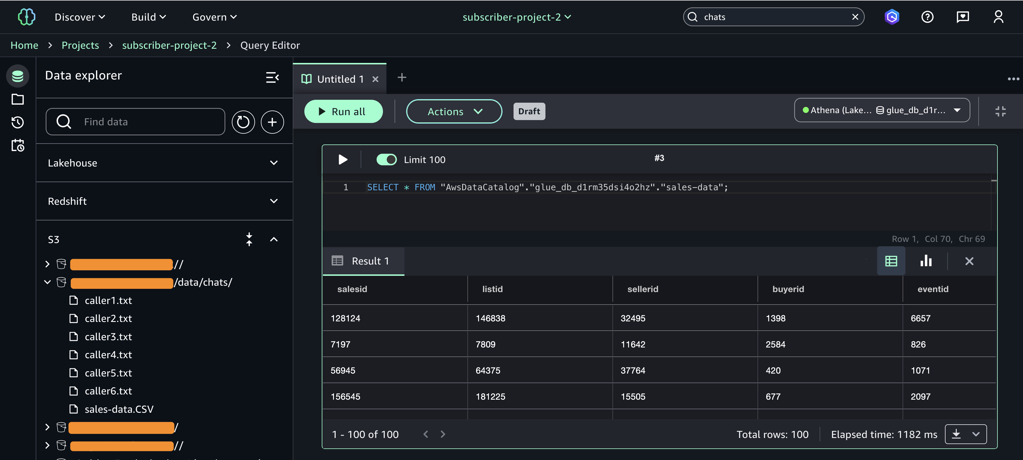
With this access granted through S3 Access Grants, you can seamlessly incorporate S3 data into my workflows—analyzing it in notebooks, combining it with structured data in the lakehouse and Amazon Redshift for comprehensive analytics. You can access unstructured data such as documents, images in JupyterLab notebooks to train ML models, or generate queryable insights.
Automatic data onboarding from your lakehouse
This integration automatically onboards all your lakehouse datasets into SageMaker Catalog. The key benefit for you is to bring AWS Glue Data Catalog (GDC) datasets into SageMaker Catalog, eliminating manual setup for cataloging, sharing, and governing them centrally.
This integration requires an existing lakehouse setup with Data Catalog containing your structured datasets.
When you set up a SageMaker domain, SageMaker Catalog automatically ingests metadata from all lakehouse databases and tables. This means you can immediately explore and use these datasets from within SageMaker Unified Studio without any configuration.
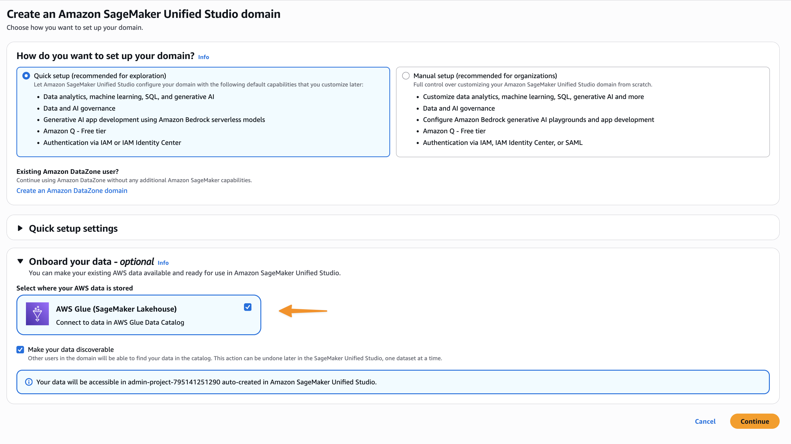
The integration helps you to start managing, governing, and consuming these assets from within SageMaker Unified Studio, applying the same governance policies and access controls you can use for other data types while unifying technical and business metadata.
Additional things to know
Here are a couple of things to note:
- Availability – These integrations are available in all commercial AWS Regions where Amazon SageMaker is supported.
- Pricing – Standard SageMaker Unified Studio, QuickSight, and Amazon S3 pricing applies. No additional charges for the integrations themselves.
- Documentation – You can find complete setup guides in the SageMaker Unified Studio Documentation.
Get started with these new integrations through the Amazon SageMaker Unified Studio console.
Happy building!
— Donnie
AWS Free Tier update: New customers can get started and explore AWS with up to $200 in credits
Post Syndicated from Channy Yun (윤석찬) original https://aws.amazon.com/blogs/aws/aws-free-tier-update-new-customers-can-get-started-and-explore-aws-with-up-to-200-in-credits/
When you’re new to Amazon Web Services (AWS), you can get started with AWS Free Tier to learn about AWS services, gain hands-on experience, and build applications. You can explore the portfolio of services without incurring costs, making it even easier to get started with AWS.
Today, we’re announcing some enhancements to the AWS Free Tier program, offering up to $200 in AWS credits that can be used across AWS services. You’ll receive $100 in AWS credits upon sign-up and can earn an additional $100 in credits by using services such as Amazon Elastic Compute Cloud (Amazon EC2), Amazon Relational Database Service (Amazon RDS), AWS Lambda, Amazon Bedrock, and AWS Budgets.
The enhanced AWS Free Tier program offers two options during sign-up: a free account plan and a paid account plan. The free account plan ensures you won’t incur any charges until you upgrade to a paid plan. The free account plan expires after 6 months or when you exhaust your credits, whichever comes first.
While on the free account plan, you won’t be able to use some services typically used by large enterprises. You can upgrade to a paid plan at any time to continue building on AWS. When you upgrade, you can still use any unused credits for any eligible service usage for up to 12 months from your initial sign-up date.

When you choose the paid plan, AWS will automatically apply your Free Tier credits to the use of eligible services in your AWS bills. For usage that exceeds the credits, you’re charged with the on-demand pricing.
Get up to $200 credits in action
When you sign up for either a free plan or a paid plan, you’ll receive $100 credit. You can also earn an additional $20 credits for each of these five AWS service activities you complete:
- Amazon EC2 – You’ll learn how to launch an EC2 instance and terminate it.
- Amazon RDS – You’ll learn the basic configuration options for launching an RDS database.
- AWS Lambda – You’ll learn to build a straightforward web application consisting of a Lambda function with a function URL.
- Amazon Bedrock – You’ll learn how to submit a prompt to generate a response in the Amazon Bedrock text playground.
- AWS Budgets – You’ll learn how to set a budget that alerts you when you exceed your budgeted cost amount.
You can see the credit details in the Explore AWS widget in the AWS Management Console.

These activities are designed to expose customers to important building blocks of AWS, including cost and usage that show up in the AWS Billing Console. These charges are deducted from your Free Tier credits and help teach new AWS users about selecting the appropriate instance sizes to minimize your costs.
Choose Set up a cost budget using AWS Budgets to earn your first $20 credits. It redirects to the AWS Billing and Cost Management console.
To create your first budget, choose Use a template (simplified) and Monthly cost budget to notify you if you exceed, or are forecasted to exceed, the budget amount.

When you choose the Customize (advanced) setup option, you can customize a budget to set parameters specific to your use case, scope of AWS services or AWS Regions, the time period, the start month, and specific accounts.
After you successfully create your budget, your begin receiving alerts when your spend exceeds your budgeted amount.

You can go to the Credits page in the left navigation pane in the AWS Billing and Cost Management Console to confirm your $20 in credits. Please note, it can take up to 10 minutes for your credits to appear.

You can receive an additional $80 by completing the remaining four activities. Now you can use up to $200 in credits to learn AWS services and build your first application.
Things to know
Here are some of things to know about the enhanced AWS Free Tier program:
- Notifications – We’ll send an email alert when 50 percent, 25 percent, or 10 percent of your AWS credits remain. We’ll also send notifications to the AWS console and your email inbox when you have 15 days, 7 days, and 2 days left in your 6-month free period. After your free period ends, we’ll send you an email with instructions on how to upgrade to a paid plan. You’ll have 90 days to reopen your account by upgrading to a paid plan.
- AWS services – The free account can access parts of AWS services including over 30 services that offer always-free tier. The paid account can access all AWS services. For more information, visit AWS Free Tier page.
- Legacy Free Tier – If your AWS account was created before July 15, 2025, you’ll continue to be in the legacy Free Tier program, where you can access short-term trials, 12-month trials, and always free tier services. The always-free tier is available under both the new Free Tier program and the legacy Free Tier program.
Now available
The new AWS Free Tier features are generally available in all AWS Regions, except the AWS GovCloud (US) Regions and the China Regions. To learn more, visit the AWS Free Tier page and AWS Free Tier Documentation.
Give the new AWS Free Tier a try by signing up today, and send feedback to AWS re:Post for AWS Free Tier or through your usual AWS Support contacts.
— Channy
Monitor and debug event-driven applications with new Amazon EventBridge logging
Post Syndicated from Donnie Prakoso original https://aws.amazon.com/blogs/aws/monitor-and-debug-event-driven-applications-with-new-amazon-eventbridge-logging/
Starting today, you can use enhanced logging capability in Amazon EventBridge to monitor and debug your event-driven applications with comprehensive logs. These new enhancements help improve how you monitor and troubleshoot event flows.
Here’s how you can find this new capability on the Amazon EventBridge console:

The new observability capabilities address microservices and event-driven architecture monitoring challenges by providing comprehensive event lifecycle tracking. EventBridge now generates detailed log entries every time a matched event against rules is published, delivered to subscribers, or encounters failures and retries.
You gain visibility into the complete event journey with detailed information about successes, failures, and status codes that make identifying and diagnosing issues straightforward. What used to take hours of trial-and-error debugging now takes minutes with detailed event lifecycle tracking and built-in query tools.
Using Amazon EventBridge enhanced observability
Let me walk you through a demonstration that showcases the logging capability in Amazon EventBridge.
I can enable logging for an existing event bus or when creating a new custom event bus. First, I navigate to the EventBridge console and choose Event buses in the left navigation pane. In Custom event bus, I choose Create event bus.

I can see this new capability in the Logs section. I have three options to configure the Log destination: Amazon CloudWatch Logs, Amazon Data Firehose Stream, and Amazon Simple Storage Service (Amazon S3). If I want to stream my logs into a data lake, I can select Amazon Kinesis Data Firehose Stream. Logs are encrypted in transit with TLS and at rest if a customer-managed key (CMK) is provided for the event bus. CloudWatch Logs supports customer-managed keys, and Data Firehose offers server-side encryption for downstream destinations.
For this demo, I select CloudWatch logs and S3 logs.

I can also choose Log level, from Error, Info, or Trace. I choose Trace and select Include execution data because I need to review the payloads. You need to be mindful as logging payload data may contain sensitive information, and this setting applies to all log destinations you select. Then, I configure two destinations, one each for CloudWatch log group and S3 logs. Then I choose Create.

After logging is enabled, I can start publishing test events to observe the logging behavior.

For the first scenario, I’ve built an AWS Lambda function and configured this Lambda function as a target.

I navigate to my event bus to send a sample event by choosing Send events.

Here’s the payload that I use:
{
  "Source": "ecommerce.orders",
  "DetailType": "Order Placed",
  "Detail": {
    "orderId": "12345",
    "customerId": "cust-789",
    "amount": 99.99,
    "items": [
      {
        "productId": "prod-456",
        "quantity": 2,
        "price": 49.99
      }
    ]
  }
}
After I sent the sample event, I can see the logs are available in my S3 bucket.

I can also see the log entries appearing in the Amazon CloudWatch logs. The logs show the event lifecycle, from EVENT_RECEIPT to SUCCESS. Learn more about the complete event lifecycle on TBD:DOC_PAGE.

Now, let’s evaluate these logs. For brevity, I only include a few logs and have redacted them for readability. Here’s the log from when I triggered the event:
{
    "resource_arn": "arn:aws:events:us-east-1:123:event-bus/demo-logging",
    "message_timestamp_ms": 1751608776896,
    "event_bus_name": "demo-logging",
// REDACTED FOR BREVITY //
    "message_type": "EVENT_RECEIPT",
    "log_level": "TRACE",
    "details": {
        "caller_account_id": "123",
        "source_time_ms": 1751608775000,
        "source": "ecommerce.orders",
        "detail_type": "Order Placed",
        "resources": [],
        "event_detail": "REDACTED FOR BREVITY"
    }
}
Here’s the log when the event was successfully invoked:
{
    "resource_arn": "arn:aws:events:us-east-1:123:event-bus/demo-logging",
    "message_timestamp_ms": 1751608777091,
    "event_bus_name": "demo-logging",
// REDACTED FOR BREVITY //
    "message_type": "INVOCATION_SUCCESS",
    "log_level": "INFO",
    "details": {
// REDACTED FOR BREVITY //
        "total_attempts": 1,
        "final_invocation_status": "SUCCESS",
        "ingestion_to_start_latency_ms": 105,
        "ingestion_to_complete_latency_ms": 183,
        "ingestion_to_success_latency_ms": 183,
        "target_duration_ms": 53,
        "target_response_body": "<REDACTED FOR BREVITY>",
        "http_status_code": 202
    }
}
The additional log entries include rich metadata that makes troubleshooting straightforward. For example, on a successful event, I can see the latency timing from starting to completing the event, duration for the target to finish processing, and HTTP status code.
Debugging failures with complete event lifecycle tracking
The benefit of EventBridge logging becomes apparent when things go wrong. To test failure scenarios, I intentionally misconfigure a Lambda function’s permissions and change the rule to point to a different Lambda function without proper permissions.

The attempt failed with a permanent failure due to missing permissions. The log shows it’s a FIRST attempt that resulted in NO_PERMISSIONS status.
{
    "message_type": "INVOCATION_ATTEMPT_PERMANENT_FAILURE",
    "log_level": "ERROR",
    "details": {
        "rule_arn": "arn:aws:events:us-east-1:123:rule/demo-logging/demo-order-placed",
        "role_arn": "arn:aws:iam::123:role/service-role/Amazon_EventBridge_Invoke_Lambda_123",
        "target_arn": "arn:aws:lambda:us-east-1:123:function:demo-evb-fail",
        "attempt_type": "FIRST",
        "attempt_count": 1,
        "invocation_status": "NO_PERMISSIONS",
        "target_duration_ms": 25,
        "target_response_body": "{\"requestId\":\"a4bdfdc9-4806-4f3e-9961-31559cb2db62\",\"errorCode\":\"AccessDeniedException\",\"errorType\":\"Client\",\"errorMessage\":\"User: arn:aws:sts::123:assumed-role/Amazon_EventBridge_Invoke_Lambda_123/db4bff0a7e8539c4b12579ae111a3b0b is not authorized to perform: lambda:InvokeFunction on resource: arn:aws:lambda:us-east-1:123:function:demo-evb-fail because no identity-based policy allows the lambda:InvokeFunction action\",\"statusCode\":403}",
        "http_status_code": 403
    }
}
The final log entry summarizes the complete failure with timing metrics and the exact error message.
{
    "message_type": "INVOCATION_FAILURE",
    "log_level": "ERROR",
    "details": {
        "rule_arn": "arn:aws:events:us-east-1:123:rule/demo-logging/demo-order-placed",
        "role_arn": "arn:aws:iam::123:role/service-role/Amazon_EventBridge_Invoke_Lambda_123",
        "target_arn": "arn:aws:lambda:us-east-1:123:function:demo-evb-fail",
        "total_attempts": 1,
        "final_invocation_status": "NO_PERMISSIONS",
        "ingestion_to_start_latency_ms": 62,
        "ingestion_to_complete_latency_ms": 114,
        "target_duration_ms": 25,
        "http_status_code": 403
    },
    "error": {
        "http_status_code": 403,
        "error_message": "User: arn:aws:sts::123:assumed-role/Amazon_EventBridge_Invoke_Lambda_123/db4bff0a7e8539c4b12579ae111a3b0b is not authorized to perform: lambda:InvokeFunction on resource: arn:aws:lambda:us-east-1:123:function:demo-evb-fail because no identity-based policy allows the lambda:InvokeFunction action",
        "aws_service": "AWSLambda",
        "request_id": "a4bdfdc9-4806-4f3e-9961-31559cb2db62"
    }
}
The logs provide detailed performance metrics that help identify bottlenecks. The ingestion_to_start_latency_ms: 62 shows the time from event ingestion to starting invocation, while ingestion_to_complete_latency_ms: 114 represents the total time from ingestion to completion. Additionally, target_duration_ms: 25 indicates how long the target service took to respond, helping distinguish between EventBridge processing time and target service performance.
The error message clearly states what failed, lambda:InvokeFunction action, why it failed, (no identity-based policy allows the action), which role was involved (Amazon_EventBridge_Invoke_Lambda_1428392416), and which specific resource was affected, which was indicated by the Lambda function Amazon Resource Name (ARN).
Debugging API Destinations with EventBridge Logging
One particular use case that I think EventBridge logging capability will be helpful is to debug issues with API destinations. EventBridge API destinations are HTTPS endpoints that you can invoke as the target of an event bus rule or pipe. HTTPS endpoints help you to route events from your event bus to external systems, software-as-a-service (SaaS) applications, or third-party APIs using HTTPS calls. They use connections to handle authentication and credentials, making it easy to integrate your event-driven architecture with any HTTPS-based service.
API destinations are commonly used to send events to external HTTPS endpoints and debugging failures from the external endpoint can be a challenge. These problems typically stem from changes to the endpoint authentication requirements or modified credentials.
To demonstrate this debugging capability, I intentionally configured an API destination with incorrect credentials in the connection resource.

When I send an event to this misconfigured endpoint, the enhanced logging shows the root cause of this failure.
{
    "resource_arn": "arn:aws:events:us-east-1:123:event-bus/demo-logging",
    "message_timestamp_ms": 1750344097251,
    "event_bus_name": "demo-logging",
    //REDACTED FOR BREVITY//,
    "message_type": "INVOCATION_FAILURE",
    "log_level": "ERROR",
    "details": {
        //REDACTED FOR BREVITY//,
        "total_attempts": 1,
        "final_invocation_status": "SDK_CLIENT_ERROR",
        "ingestion_to_start_latency_ms": 135,
        "ingestion_to_complete_latency_ms": 549,
        "target_duration_ms": 327,
        "target_response_body": "",
        "http_status_code": 400
    },
    "error": {
        "http_status_code": 400,
        "error_message": "Unable to invoke ApiDestination endpoint: The request failed because the credentials included for the connection are not authorized for the API destination."
    }
}
The log provides immediate clarity about the failure. The target_arn shows this involves an API destination, the final_invocation_status indicates SDK_CLIENT_ERROR, and the http_status_code of 400 , which points to a client-side issue. Most importantly, the error_message explicitly states that: Unable to invoke ApiDestination endpoint: The request failed because the credentials included for the connection are not authorized for the API destination.
This complete log sequence provides useful debugging insights because I can see exactly how the event moved through EventBridge — from event receipt, to ingestion, to rule matching, to invocation attempts. This level of detail eliminates guesswork and points directly to the root cause of the issue.
Additional things to know
Here are a couple of things to note:
- Architecture support – Logging works with all EventBridge features including custom event buses, partner event sources, and API destinations for HTTPS endpoints.
- Performance impact – Logging operates asynchronously with no measurable impact on event processing latency or throughput.
- Pricing – You pay standard Amazon S3, Amazon CloudWatch Logs or Amazon Data Firehose pricing for log storage and delivery. EventBridge logging itself incurs no additional charges. For details, visit the Amazon EventBridge pricing page .
- Availability – Amazon EventBridge logging capability is available in all AWS Regions where EventBridge is supported.
- Documentation — For more details, refer to the Amazon EventBridge monitoring and debugging Documentation.
Get started with Amazon EventBridge logging capability by visiting the EventBridge console and enabling logging on your event buses.
Happy building!
— Donnie
Introducing Amazon S3 Vectors: First cloud storage with native vector support at scale (preview)
Post Syndicated from Channy Yun (윤석찬) original https://aws.amazon.com/blogs/aws/introducing-amazon-s3-vectors-first-cloud-storage-with-native-vector-support-at-scale/
Today, we’re announcing the preview of Amazon S3 Vectors, a purpose-built durable vector storage solution that can reduce the total cost of uploading, storing, and querying vectors by up to 90 percent. Amazon S3 Vectors is the first cloud object store with native support to store large vector datasets and provide subsecond query performance that makes it affordable for businesses to store AI-ready data at massive scale.
Vector search is an emerging technique used in generative AI applications to find similar data points to given data by comparing their vector representations using distance or similarity metrics. Vectors are numerical representation of unstructured data created from embedding models. You generate vectors using embedding models for fields inside your document and store vectors into S3 Vectors to search semantically.

S3 Vectors introduces vector buckets, a new bucket type with a dedicated set of APIs to store, access, and query vector data without provisioning any infrastructure. When you create an S3 vector bucket, you organize your vector data within vector indexes, making it simple for running similarity search queries against your dataset. Each vector bucket can have up to 10,000 vector indexes, and each vector index can hold tens of millions of vectors.
After creating a vector index, when adding vector data to the index, you can also attach metadata as key-value pairs to each vector to filter future queries based on a set of conditions, for example, dates, categories, or user preferences. As you write, update, and delete vectors over time, S3 Vectors automatically optimizes the vector data to achieve the best possible price-performance for vector storage, even as the datasets scale and evolve.

S3 Vectors is also natively integrated with Amazon Bedrock Knowledge Bases, including within Amazon SageMaker Unified Studio, for building cost-effective Retrieval-Augmented Generation (RAG) applications. Through its integration with Amazon OpenSearch Service, you can lower storage costs by keeping infrequent queried vectors in S3 Vectors and then quickly move them to OpenSearch as demands increase or to support real-time, low-latency search operations.
With S3 Vectors, you can now economically store the vector embeddings that represent massive amounts of unstructured data such as images, videos, documents, and audio files, enabling scalable generative AI applications including semantic and similarity search, RAG, and build agent memory. You can also build applications to support a wide range of industry use cases including personalized recommendations, automated content analysis, and intelligent document processing without the complexity and cost of managing vector databases.
S3 Vectors in action
To create a vector bucket, choose Vector buckets in the left navigation pane in the Amazon S3 console and then choose Create vector bucket.
Enter a vector bucket name and choose the encryption type. If you don’t specify an encryption type, Amazon S3 applies server-side encryption with Amazon S3 managed keys (SSE-S3) as the base level of encryption for new vectors. You can also choose server-side encryption with AWS Key Management Service (AWS KMS) keys (SSE-KMS). To learn more about managing your vector bucket, visit S3 Vector buckets in the Amazon S3 User Guide.

Now, you can create a vector index to store and query your vector data within your created vector bucket.

Enter a vector index name and the dimensionality of the vectors to be inserted in the index. All vectors added to this index must have exactly the same number of values.
For Distance metric, you can choose either Cosine or Euclidean. When creating vector embeddings, select your embedding model’s recommended distance metric for more accurate results.

Choose Create vector index and then you can insert, list, and query vectors.

To insert your vector embeddings to a vector index, you can use the AWS Command Line Interface (AWS CLI), AWS SDKs, or Amazon S3 REST API. To generate vector embeddings for your unstructured data, you can use embedding models offered by Amazon Bedrock.
If you’re using the latest AWS Python SDKs, you can generate vector embeddings for your text using Amazon Bedrock using following code example:
# Generate and print an embedding with Amazon Titan Text Embeddings V2.
import boto3
import json

# Create a Bedrock Runtime client in the AWS Region of your choice.
bedrock= boto3.client("bedrock-runtime", region_name="us-west-2")

The text strings to convert to embeddings.
texts = [
"Star Wars: A farm boy joins rebels to fight an evil empire in space",
"Jurassic Park: Scientists create dinosaurs in a theme park that goes wrong",
"Finding Nemo: A father fish searches the ocean to find his lost son"]

embeddings=[]
#Generate vector embeddings for the input texts
for text in texts:
        body = json.dumps({
            "inputText": text
        })
        # Call Bedrock's embedding API
        response = bedrock.invoke_model(
        modelId='amazon.titan-embed-text-v2:0',  # Titan embedding model
        body=body)
        # Parse response
        response_body = json.loads(response['body'].read())
        embedding = response_body['embedding']
        embeddings.append(embedding)
Now, you can insert vector embeddings into the vector index and query vectors in your vector index using the query embedding:
# Create S3Vectors client
s3vectors_client = boto3.client('s3vectors', region_name='us-west-2')

# Insert vector embedding
s3vectors.put_vectors( vectorBucketName="channy-vector-bucket",
  indexName="channy-vector-index",
  vectors=[
{"key": "v1", "data": {"float32": embeddings[0]}, "metadata": {"id": "key1", "source_text": texts[0], "genre":"scifi"}},
{"key": "v2", "data": {"float32": embeddings[1]}, "metadata": {"id": "key2", "source_text": texts[1], "genre":"scifi"}},
{"key": "v3", "data": {"float32": embeddings[2]}, "metadata": {"id": "key3", "source_text":  texts[2], "genre":"family"}}
],
)

#Create an embedding for your query input text
# The text to convert to an embedding.
input_text = "List the movies about adventures in space"

# Create the JSON request for the model.
request = json.dumps({"inputText": input_text})

# Invoke the model with the request and the model ID, e.g., Titan Text Embeddings V2.
response = bedrock.invoke_model(modelId="amazon.titan-embed-text-v2:0", body=request)

# Decode the model's native response body.
model_response = json.loads(response["body"].read())

# Extract and print the generated embedding and the input text token count.
embedding = model_response["embedding"]

# Performa a similarity query. You can also optionally use a filter in your query
query = s3vectors.query_vectors( vectorBucketName="channy-vector-bucket",
  indexName="channy-vector-index",
  queryVector={"float32":embedding},
  topK=3,
  filter={"genre":"scifi"},
  returnDistance=True,
  returnMetadata=True
  )
results = query["vectors"]
print(results)
To learn more about inserting vectors into a vector index, or listing, querying, and deleting vectors, visit S3 vector buckets and S3 vector indexes in the Amazon S3 User Guide. Additionally, with the S3 Vectors embed command line interface (CLI), you can create vector embeddings for your data using Amazon Bedrock and store and query them in an S3 vector index using single commands. For more information, see the S3 Vectors Embed CLI GitHub repository.
Integrate S3 Vectors with other AWS services
S3 Vectors integrates with other AWS services such as Amazon Bedrock, Amazon SageMaker, and Amazon OpenSearch Service to enhance your vector processing capabilities and provide comprehensive solutions for AI workloads.
Create Amazon Bedrock Knowledge Bases with S3 Vectors
You can use S3 Vectors in Amazon Bedrock Knowledge Bases to simplify and reduce the cost of vector storage for RAG applications. When creating a knowledge base in the Amazon Bedrock console, you can choose the S3 vector bucket as your vector store option.
In Step 3, you can choose the Vector store creation method either to create an S3 vector bucket and vector index or choose the existing S3 vector bucket and vector index that you’ve previously created.

For detailed step-by-step instructions, visit Create a knowledge base by connecting to a data source in Amazon Bedrock Knowledge Bases in the Amazon Bedrock User Guide.
Using Amazon SageMaker Unified Studio
You can create and manage knowledge bases with S3 Vectors in Amazon SageMaker Unified Studio when you build your generative AI applications through Amazon Bedrock. SageMaker Unified Studio is available in the next generation of Amazon SageMaker and provides a unified development environment for data and AI, including building and texting generative AI applications that use Amazon Bedrock knowledge bases.

You can choose your knowledge bases using the S3 Vectors created through Amazon Bedrock when you build generative AI applications. To learn more, visit Add a data source to your Amazon Bedrock app in the Amazon SageMaker Unified Studio User Guide.
Export S3 vector data to Amazon OpenSearch Service
You can balance cost and performance by adopting a tiered strategy that stores long-term vector data cost-effectively in Amazon S3 while exporting high priority vectors to OpenSearch for real-time query performance.
This flexibility means your organizations can access OpenSearch’s high performance (high QPS, low latency) for critical, real-time applications, such as product recommendations or fraud detection, while keeping less time-sensitive data in S3 Vectors.
To export your vector index, choose Advanced search export, then choose Export to OpenSearch in the Amazon S3 console.

Then, you will be brought to the Amazon OpenSearch Service Integration console with a template for S3 vector index export to OpenSearch vector engine. Choose Export with pre-selected S3 vector source and a service access role.

It will start the steps to create a new OpenSearch Serverless collection and migrate data from your S3 vector index into an OpenSearch knn index.
Choose the Import history in the left navigation pane. You can see the new import job that was created to make a copy of vector data from your S3 vector index into the OpenSearch Serverless collection.

Once the status changes to Complete, you can connect to the new OpenSearch serverless collection and query your new OpenSearch knn index.
To learn more, visit Creating and managing Amazon OpenSearch Serverless collections in the Amazon OpenSearch Service Developer Guide.
Now available
Amazon S3 Vectors, and its integrations with Amazon Bedrock, Amazon OpenSearch Service, and Amazon SageMaker are now in preview in the US East (N. Virginia), US East (Ohio), US West (Oregon), Europe (Frankfurt), and Asia Pacific (Sydney) Regions.
Give S3 Vectors a try in the Amazon S3 console today and send feedback to AWS re:Post for Amazon S3 or through your usual AWS Support contacts.
— Channy
Amazon S3 Metadata now supports metadata for all your S3 objects
Post Syndicated from Sébastien Stormacq original https://aws.amazon.com/blogs/aws/amazon-s3-metadata-now-supports-metadata-for-all-your-s3-objects/
Amazon S3 Metadata now provides complete visibility into all your existing objects in your Amazon Simple Storage Service (Amazon S3) buckets, expanding beyond new objects and changes. With this expanded coverage, you can analyze and query metadata for your entire S3 storage footprint.
Today, many customers rely on Amazon S3 to store unstructured data at scale. To understand what’s in a bucket, you often need to build and maintain custom systems that scan for objects, track changes, and manage metadata over time. These systems are expensive to maintain and hard to keep up to date as data grows.
Since the launch of S3 Metadata at re:Invent 2024, you’ve been able to query new and updated object metadata using metadata tables instead of relying on Amazon S3 Inventory or object-level APIs such as ListObjects, HeadObject, and GetObject—which can introduce latency and impact downstream workflows.
To make it easier for you to work with this expanded metadata, S3 Metadata introduces live inventory tables that work with familiar SQL-based tools. After your existing objects are backfilled into the system, any updates like uploads or deletions typically appear within an hour in your live inventory tables.
With S3 Metadata live inventory tables, you get a fully managed Apache Iceberg table that provides a complete and current snapshot of the objects and their metadata in your bucket, including existing objects, thanks to backfill support. These tables are refreshed automatically within an hour of changes such as uploads or deletions, so you stay up to date. You can use them to identify objects with specific properties—like unencrypted data, missing tags, or particular storage classes—and to support analytics, cost optimization, auditing, and governance.
S3 Metadata journal tables, previously known as S3 Metadata tables, are automatically enabled when you configure live inventory tables, provide a near real-time view of object-level changes in your bucket—including uploads, deletions, and metadata updates. These tables are ideal for auditing activity, tracking the lifecycle of objects, and generating event-driven insights. For example, you can use them to find out which objects were deleted in the past 24 hours, identify the requester making the most PUT operations, or monitor updates to object metadata over time.
S3 Metadata tables are created in a namespace name that is similar to your bucket name for easier discovery. The tables are stored in AWS system table buckets, grouped by account and Region. After you enable S3 Metadata for a general purpose S3 bucket, the system creates and maintains these tables for you. You don’t need to manage compaction or garbage collection processes—S3 Tables takes care of table maintenance tasks in the background.
These new tables help avoid waiting for metadata discovery before processing can begin, making them ideal for large-scale analytics and machine learning (ML) workloads. By querying metadata ahead of time, you can schedule GPU jobs more efficiently and reduce idle time in compute-intensive environments.
Let’s see how it works
To see how this works in practice, I configure S3 Metadata for a general purpose bucket using the AWS Management Console.

After choosing a general purpose bucket, I choose the Metadata tab, then I choose Create metadata configuration.
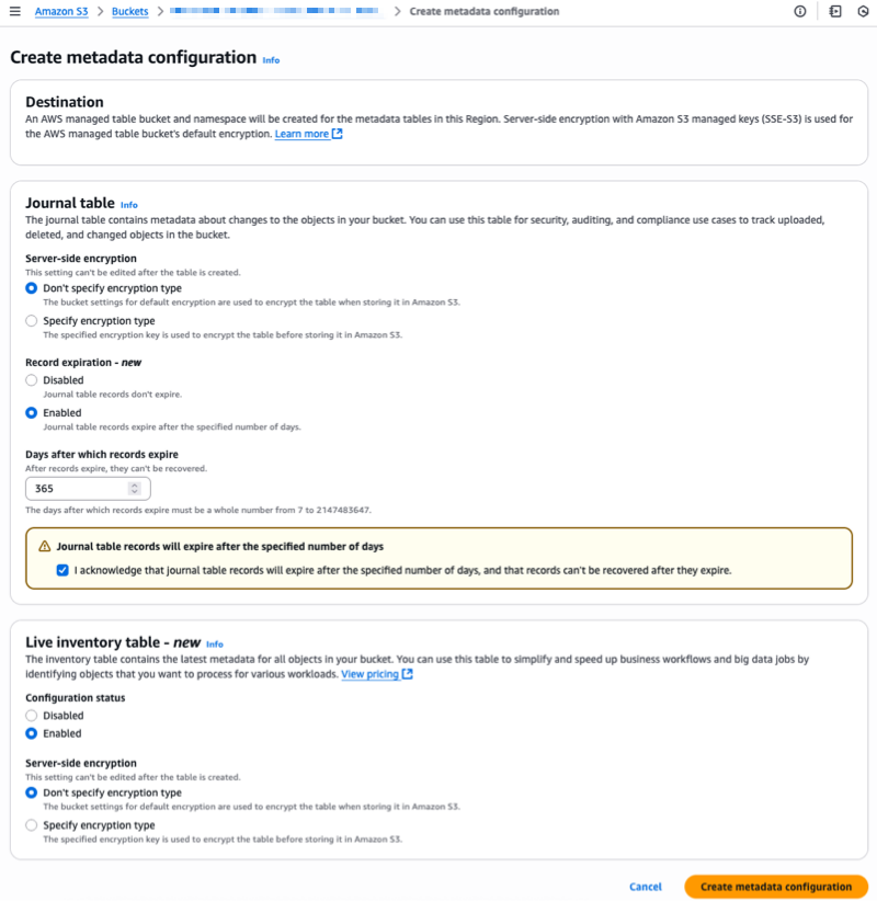 For Journal table, I can choose the Server-side encryption option and the Record expiration period. For Live Inventory table, I choose Enabled and I can select the Server-side encryption options.
I configure Record expiration on the journal table. Journal table records expire after the specified number of days, 365 days (one year) in my example.
Then, I choose Create metadata configuration.
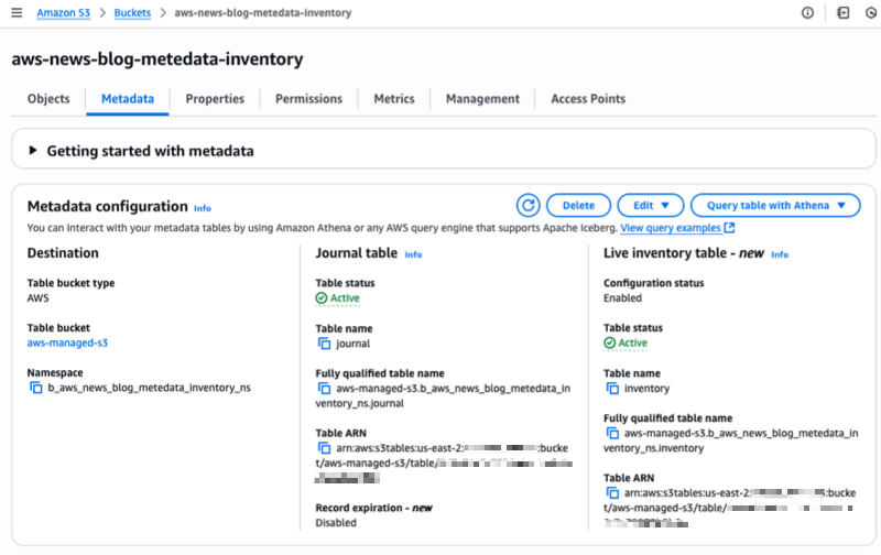
S3 Metadata creates the live inventory table and journal table. In the Live Inventory table section, I can observe the Table status: the system immediately starts to backfill the table with existing object metadata. It can take between minutes to hours. The exact time depends on the quantity of objects you have in your S3 bucket.
While waiting, I also upload and delete objects to generate data in the journal table.
Then, I navigate to Amazon Athena to start querying the new tables.
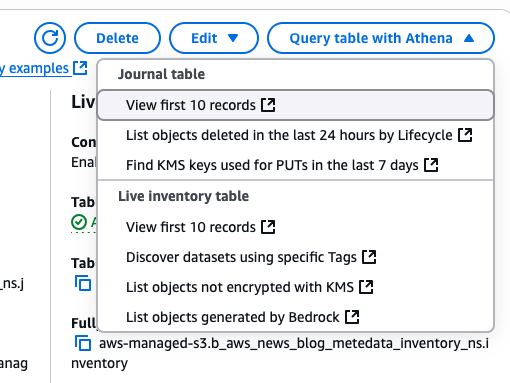
I choose Query table with Athena to start querying the table. I can choose between a couple of default queries on the console.
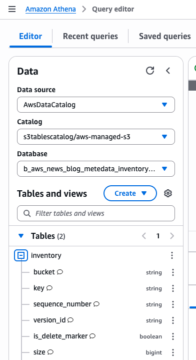
In Athena, I observe the structure of the tables in the AWSDataCatalog Data source and I start with a short query to check how many records are available in the journal table. I already have 6,488 entries:
SELECT count(*) FROM "b_aws_news_blog_metadata_inventory_ns"."journal";

# _col0
1 6488
Here are a couple of example queries I tried on the journal table:
# Query deleted objects in last 24 hours
# Use is_delete_marker=true for versioned buckets and record_type='DELETE' otherwise
SELECT bucket, key, version_id, last_modified_date
FROM "s3tablescatalog/aws-managed-s3"."b_aws_news_blog_metadata_inventory_ns"."journal"
WHERE last_modified_date >= (current_date - interval '1' day) AND is_delete_marker = true;

# bucket key version_id last_modified_date is_delete_marker
1 aws-news-blog-metadata-inventory .build/index-build/arm64-apple-macosx/debug/index/store/v5/records/G0/NSURLSession.h-JET61D329FG0
2 aws-news-blog-metadata-inventory .build/index-build/arm64-apple-macosx/debug/index/store/v5/records/G5/cdefs.h-PJ21EUWKMWG5
3 aws-news-blog-metadata-inventory .build/index-build/arm64-apple-macosx/debug/index/store/v5/records/FX/buf.h-25EDY57V6ZXFX
4 aws-news-blog-metadata-inventory .build/index-build/arm64-apple-macosx/debug/index/store/v5/records/G6/NSMeasurementFormatter.h-3FN8J9CLVMYG6
5 aws-news-blog-metadata-inventory .build/index-build/arm64-apple-macosx/debug/index/store/v5/records/G8/NSXMLDocument.h-1UO2NUJK0OAG8

# Query recent PUT requests IP addresses
SELECT source_ip_address, count(source_ip_address)
FROM "s3tablescatalog/aws-managed-s3"."b_aws_news_blog_metadata_inventory_ns"."journal"
GROUP BY source_ip_address;

#	source_ip_address	_col1
1	my_laptop_IP_address	12488

# Query S3 Lifecycle expired objects in last 7 days
SELECT bucket, key, version_id, last_modified_date, record_timestamp
FROM "s3tablescatalog/aws-managed-s3"."b_aws_news_blog_metadata_inventory_ns"."journal"
WHERE requester = 's3.amazonaws.com' AND record_type = 'DELETE' AND record_timestamp > (current_date - interval '7' day);

(not applicable to my demo bucket)
The results helped me track the specific objects that were removed, including their timestamps.
Now, I look at the live inventory table:
# Distribution of object tags
SELECT object_tags, count(object_tags)
FROM "s3tablescatalog/aws-managed-s3"."b_aws_news_blog_metadata_inventory_ns"."inventory"
GROUP BY object_tags;

# object_tags    _col1
1 {Source=Swift} 1
2 {Source=swift} 1
3 {}             12486

# Query storage class and size for specific tags
SELECT storage_class, count(*) as count, sum(size) / 1024 / 1024 as usage
FROM "s3tablescatalog/aws-managed-s3"."b_aws_news_blog_metadata_inventory_ns"."inventory"
GROUP BY object_tags['pii=true'], storage_class;

# storage_class count   usage
1 STANDARD      124884  165

# Find objects with specific user defined metadata
SELECT key, last_modified_date, user_metadata
FROM "s3tablescatalog/aws-managed-s3"."b_aws_news_blog_metadata_inventory_ns"."inventory"
WHERE cardinality(user_metadata) > 0 ORDER BY last_modified_date DESC;

(not applicable to my demo bucket)
These are just a few examples of what is possible with S3 Metadata. Your preferred queries will depend on your use cases. Refer to Analyzing Amazon S3 Metadata with Amazon Athena and Amazon QuickSight in the AWS Storage Blog for more examples.
Pricing and availability
S3 Metadata live inventory and journal tables are available today in US East (Ohio, N. Virginia) and US West (N. California).
The journal tables are charged $0.30 per million updates. This is a 33 percent drop from our previous price.
For inventory tables, there’s a one-time backfill cost of $0.30 for a million objects to set up the table and generate metadata for existing objects. There are no additional costs if your bucket has less than one billion objects. For buckets with more than a billion objects, there is a monthly fee of $0.10 per million objects per month.
As usual, the Amazon S3 pricing page has all the details.
With S3 Metadata live inventory and journal tables, you can reduce the time and effort required to explore and manage large datasets. You get an up-to-date view of your storage and a record of changes, and both are available as Iceberg tables you can query on demand. You can discover data faster, power compliance workflows, and optimize your ML pipelines.
You can get started by enabling metadata inventory on your S3 bucket through the AWS console, AWS Command Line Interface (AWS CLI), or AWS SDKs. When they’re enabled, the journal and live inventory tables are automatically created and updated. To learn more, visit the S3 Metadata Documentation page.
TwelveLabs video understanding models are now available in Amazon Bedrock
Post Syndicated from Channy Yun (윤석찬) original https://aws.amazon.com/blogs/aws/twelvelabs-video-understanding-models-are-now-available-in-amazon-bedrock/
Earlier this year, we preannounced that TwelveLabs video understanding models were coming to Amazon Bedrock. Today, we’re announcing the models are now available for searching through videos, classifying scenes, summarizing, and extracting insights with precision and reliability.
TwelveLabs has introduced Marengo, a video embedding model proficient at performing tasks such as search and classification, and Pegasus, a video language model that can generate text based on video data. These models are trained on Amazon SageMaker HyperPod to deliver groundbreaking video analysis that provides text summaries, metadata generation, and creative optimization.
With the TwelveLabs models in Amazon Bedrock, you can find specific moments using natural language video search capabilities like “show me the first touchdown of the game” or “find the scene where the main characters first meet” and instantly jump to those exact moments. You can also build applications to understand video content by generating descriptive text such as titles, topics, hashtags, summaries, chapters, or highlights for discovering insights and connections without requiring predefined labels or categories.
For example, you can find recurring themes in customer feedback or spot product usage patterns that weren’t obvious before. Whether you have hundreds or thousands of hours of video content, you can now transform that entire library into a searchable knowledge resource while maintaining enterprise-grade security and performance.
Let’s take a look at the Marengo and Pegasus videos that TwelveLabs has published.
You can transform video workflows with these models across industries. Media producers and editors can instantly locate specific scenes or dialogue, which means you can focus on storytelling rather than sifting through hours of footage. Marketing teams are streamlining their advertising workflows by quickly personalizing content to resonate with various audiences, while security teams are using the technology to proactively identify potential risks by spotting patterns across multiple video feeds.
Getting started with TwelveLabs models in Amazon Bedrock
Before getting started, if you’re new to using TwelveLabs models, go to the Amazon Bedrock console and choose Model access in the bottom left navigation pane. To access the latest TwelveLabs models, request access for Marengo Embed 2.7 and Pegasus 1.2 in TwelveLabs.
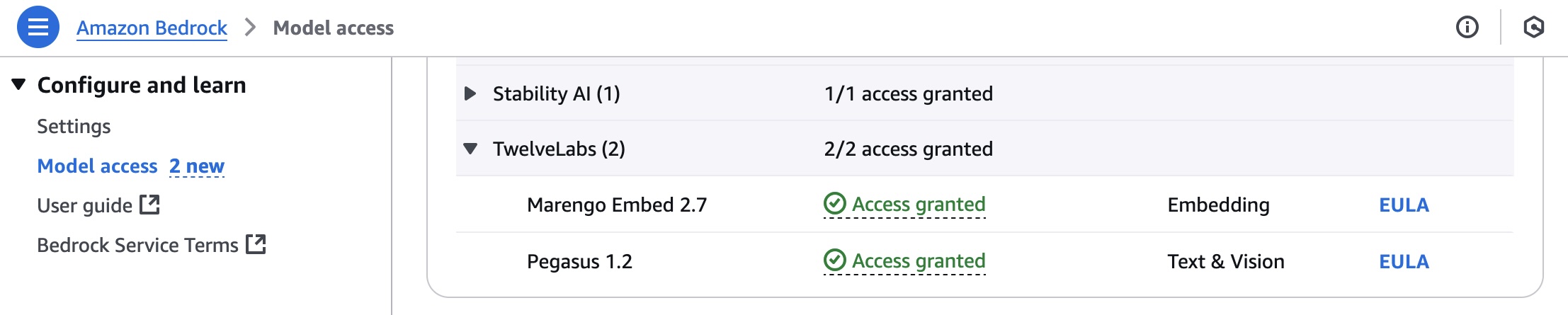
To use TwelveLabs models in Amazon Bedrock, choose Chat/Text Playground under Test in the left navigation pane. Choose Select model, select TwelveLabs as the category and Pegasus as the model, and then choose Apply.
For searching or generating text from your video, you should upload your video to an Amazon Simple Storage Service (Amazon S3) bucket or input Base64-formatted video string.
I will use a sample video generated with Amazon Nova Reel with a prompt: “A cute raccoon playing guitar underwater.”
Enter the S3 URI of your uploaded video and the S3 Bucket Owner, and then run your prompt: “Tell me about the video by timeline”.
You can get following model response:
The video opens with an underwater scene featuring a sandy seabed and swaying seaweed, creating a serene atmosphere. At around 5 seconds, a raccoon appears, swimming towards the camera with a curious expression. By 10 seconds, the raccoon is seen swimming near the seabed. The focus then shifts to a group of koi fish swimming gracefully near the seabed from 11 to 13 seconds.
At 14 seconds, the scene transitions to an ukulele resting on the seabed, with the camera zooming in to highlight its details. The raccoon reappears at 20 seconds, swimming among the koi fish, and by 23 seconds, it begins to play the ukulele. The raccoon continues to play the ukulele from 29 to 41 seconds, with the koi fish swimming around it, adding a lively and colorful touch to the underwater setting.
From 42 to 49 seconds, the raccoon is shown playing the ukulele with the koi fish swimming around it. The video concludes with a screen displaying "Video generated with Amazon Novo Reel 1.1" and "Available in Amazon Bedrock" from 50 to 54 seconds, followed by the AWS logo from 55 to 57 seconds.
The TwelveLabs models can be easily integrated into your applications using the Amazon Bedrock Converse API, which provides a unified interface for conversational AI interactions.
Here’s an example of how to use the AWS SDK for Python (Boto3) with the TwelveLabs Pegasus model:
import boto3
import json
import os

AWS_REGION = "us-east-1"
MODEL_ID = "twelvelabs.pegasus-1-2-v1:0"
VIDEO_PATH = "sample.mp4"

def read_file(file_path: str) -> bytes:
    """Read a file in binary mode."""
    try:
        with open(file_path, 'rb') as file:
            return file.read()
    except Exception as e:
        raise Exception(f"Error reading file {file_path}: {str(e)}")

bedrock_runtime = boto3.client(
    service_name="bedrock-runtime",
    region_name=AWS_REGION
)

request_body = {
    "messages": [
        {
            "role": "user",
            "content": [
                {
                    "inputPrompt": "tell me about the video",
                    "mediaSource: {
                        "base64String": read_file(VIDEO_PATH)
                    }
                },
            ],
        }
    ]
}

response = bedrock_runtime.converse(
    modelId=MODEL_ID,
    messages=request_body["messages"]
)

print(response["output"]["message"]["content"][-1]["text"])
The TwelveLabs Marengo Embed 2.7 model generates vector embeddings from video, text, audio, or image inputs. These embeddings can be used for similarity search, clustering, and other machine learning (ML) tasks. The model supports asynchronous inference through the Bedrock AsyncInvokeModel API.
For video source, you can request JSON format for the TwelveLabs Marengo Embed 2.7 model using the AsyncInvokeModel API.
{
    "modelId": "twelvelabs.marengo-embed-2.7",
    "modelInput": {
        "inputType": "video",
        "mediaSource": {
            "s3Location": {
                "uri": "s3://your-video-object-s3-path",
                "bucketOwner": "your-video-object-s3-bucket-owner-account"
            }
        }
    },
    "outputDataConfig": {
        "s3OutputDataConfig": {
            "s3Uri": "s3://your-bucket-name"
        }
    }
}
You can get a response delivered to the specified S3 location.
{
    "embedding": [0.345, -0.678, 0.901, ...],
    "embeddingOption": "visual-text",
    "startSec": 0.0,
    "endSec": 5.0
}
To help you get started, check out a broad range of code examples for multiple use cases and a variety of programming languages. To learn more, visit TwelveLabs Pegasus 1.2 and TwelveLabs Marengo Embed 2.7 in the AWS Documentation.
Now available
TwelveLabs models are generally available today in Amazon Bedrock: the Marengo model in the US East (N. Virginia), Europe (Ireland), and Asia Pacific (Seoul) Region, and the Pegasus model in US West (Oregon), and Europe (Ireland) Region accessible with cross-Region inference from US and Europe Regions. Check the full Region list for future updates. To learn more, visit the TwelveLabs in Amazon Bedrock product page and the Amazon Bedrock pricing page.
Give TwelveLabs models a try on the Amazon Bedrock console today, and send feedback to AWS re:Post for Amazon Bedrock or through your usual AWS Support contacts.
— Channy
This Raspberry Pi 5 Case Has a Secret Feature!
Post Syndicated from Crosstalk Solutions original https://www.youtube.com/shorts/N1i_3ObpmsE
Introducing Jobs in Amazon SageMaker
Post Syndicated from Chiho Sugimoto original https://aws.amazon.com/blogs/big-data/introducing-jobs-in-amazon-sagemaker/
Processing large volumes of data efficiently is critical for businesses, and so data engineers, data scientists, and business analysts need reliable and scalable ways to run data processing workloads. The next generation of Amazon SageMaker is the center for all your data, analytics, and AI. Amazon SageMaker Unified Studio is a single data and AI development environment where you can find and access all of the data in your organization and act on it using the best tools across any use case.
We’re excited to announce a new data processing job experience for Amazon SageMaker. Jobs are a common concept widely used in existing AWS services such as Amazon EMR and AWS Glue. With this launch, you can now build jobs in SageMaker to process large volumes of data. Jobs can be built using your preferred tool. For example, you can create jobs from extract, transform, and load (ETL) scripts coded in the Unified Studio code editor, code interactively in a Unified Studio Notebooks, or create jobs visually using the Unified Studio Visual ETL editor. After being created, data processing jobs can be set to run on demand, scheduled using the built in scheduler, or orchestrated with SageMaker workflows. You can monitor the status of your data processing jobs and view run history showing status, logs, and performance metrics. When jobs encounter failures, you can use generative AI troubleshooting to automatically analyze errors and receive detailed recommendations to resolve issues quickly. Together, you can use these capabilities to author, manage, operate, and monitor data processing workloads across your organization. The new experience provides an experience that’s consistent with other AWS analytics services such as AWS Glue.
This post demonstrates how the new jobs experience works in SageMaker Unified Studio.
Prerequisites
To get started, you must have the following prerequisites in place:
- An AWS account
- A SageMaker Unified Studio domain
- A SageMaker Unified Studio project with an Data analytics and AI-ML model development project profile
Example use case
A global apparel ecommerce retailer processes thousands of customer reviews daily across multiple marketplaces. They need to transform their raw review data into actionable insights to improve their product offerings and customer experience. Using SageMaker Unified Studio visual ETL editor, we’ll demonstrate how to transform raw review data into structured analytical datasets that enable market-specific performance analysis and product quality monitoring.
Create and run a visual job
In this section, you’ll create a Visual ETL Job that processes the review data from a Parquet file in Amazon Simple Storage Service Amazon S3. The job transforms the data using SQL queries and saves the results back to S3 buckets. Complete the following steps to create a Visual ETL Job:
- On the SageMaker Unified Studio console, on the top menu, choose Build.
- Under DATA ANALYSIS & INTEGRATION, choose Data processing jobs.
- Choose Create Visual ETL Job.

You’ll be directed to the Visual ETL editor, where you can create ETL jobs. You can use this editor to design data transformation pipelines by connecting source nodes, transformation nodes, and target nodes.
- On the top left, choose the plus (+) icon in the circle. Under Data sources, select Amazon S3.
- Select the Amazon S3 source node and enter the following values:
- S3 URI:
s3://aws-bigdata-blog/generated_synthetic_reviews/data/product_category=Apparel/ - Format: Parquet
- S3 URI:
- Select Update node.
- Choose the plus (+) icon in the circle to the right of the Amazon S3 source node. Under Transforms, select SQL query.
- Enter the following query statement and select Update node.
- Choose the plus (+) icon to the right of the SQL Query node. Under Data target, select Amazon S3.
- Select the Amazon S3 target node and enter the following values:
- S3 URI: Choose the Amazon S3 location from the project overview page and add the suffix “
/output/rating_analysis/”. For example,s3://<bucket-name>/<domainId>/<projectId>/output/rating_analysis/ - Format: Parquet
- Compression: Snappy
- Partition keys: review_date
- Mode: Append
- S3 URI: Choose the Amazon S3 location from the project overview page and add the suffix “
- Select Update node.

Next, add another SQL query node connected to the same Amazon S3 data source. This node performs a SQL query transformations and outputs the results to a separate S3 location.
- On the top left, choose the plus (+) icon in the circle. Under Transforms, select SQL query, and connect the Amazon S3 source node.
- Enter the following query statement and select Update node.
- Choose the plus (+) icon to the right of the SQL Query node. Under Data target, select Amazon S3.
- Select the Amazon S3 target node and enter the following values:
- S3 URI: Choose the Amazon S3 location from the project overview page and add suffix “
/output/product_analysis/”. For example,s3://<bucket-name>/<domainId>/<projectId>/output/product_analysis/ - Format: Parquet
- Compression: Snappy
- Partition keys: marketplace
- Mode: Append
- S3 URI: Choose the Amazon S3 location from the project overview page and add suffix “
- Select Update node.
At this point, your end-to-end visual job should look like the following image. The next step is to save this job to the project and run the job.

- On the top right, choose Save to project to save the draft job. You can optionally change the name and add a description.
- Choose Save.
- On the top right, choose Run.
This will start running your Visual ETL job. You can monitor the list of job runs by selecting View runs in the top middle of the screen.

Create and run a code based job
In addition to creating jobs through the Visual ETL Editor, you can create jobs using a code-based approach by specifying Python script or Notebook files. When you specify a Notebook file, it automatically converts to a Python script to create the job. Here, you’ll create a notebook in JupyterLab within SageMaker Unified Studio, save it to the project repository, and then create a code-based job from that notebook. First, create a Notebook.
- On the SageMaker Unified Studio console, on the top menu, choose Build.
- Under IDE & APPLICATIONS, select JupyterLab.
- Select Python 3 under Notebook.

- For the first cell, select Local Python, python, enter following code:
- For the second cell, select PySpark, project.spark.compatibility, enter following code. This performs the same processing as the Visual ETL job you created above. Replace the S3 bucket and folder names for output_path.
- Choose the File icon to save the notebook file. Enter the name of your notebook.

Save the notebook to the project’s repository.
- Choose the Git icon in the left navigation. This opens a panel where you can view the commit history and perform Git operations.
- Choose the plus (+) icon next to the files you want to commit.
- Enter a brief summary of the commit in the Summary text entry field. Optionally, enter a longer description of the commit in the Description text entry field.
- Choose Commit.
- Choose the Push committed changes icon to do a git push.

Create the Code-based Job from the Notebook file in the project repository.
- On the SageMaker Unified Studio console, on the top menu, choose Build.
- Under DATA ANALYSIS & INTEGRATION, choose Data processing jobs.
- Choose Create job from files.
- Choose Choose project files and choose Browse files.
- Select the Notebook file you created and choose Select.
Here, the Python script automatically converted from your notebook file will be displayed. Review the content.

- Choose Next.
- For Job name, enter the name of your job.
- Choose Submit to create your job.
- Choose the job you created.
- Choose Run job.
Convert existing Visual ETL flows to jobs
You can convert an existing visual ETL flow to a job by saving your existing Visual ETL flow to the project repository. Use the following steps to create a job from your existing visual ETL flow:
- On the SageMaker Unified Studio console, on the top menu, choose Build.
- Under DATA ANALYSIS & INTEGRATION, select Visual ETL editor.
- Select the existing Visual ETL flow.
- On the top right, choose Save to project to save the draft flow. You can optionally change the name and add a description.
- Choose Save.
View jobs
You can view the list of jobs in your project on the Data processing jobs page. Jobs can be filtered by mode (Visual ETL or Code).

Monitor job runs
On each job’s detail page, you can view a list of job runs in the Job runs tab. You can filter activities by job run ID, status, start time, and end time. The Job runs list shows basic attributes such as duration, resources consumed, and instance type, along with log group names and various job parameters. You can list, compare, and explore job runs history based on various attributes.

On the individual job run details page, you can view job properties and output logs from the run. When a job fails because of an error, you can see the error message at the top of the page and examine detailed error information in the output logs.

Intelligent troubleshooting with generative AI: When jobs fail, you can take advantage of generative AI troubleshooting to resolve issues quickly. SageMaker Unified Studio’s AI-powered troubleshooting automatically analyzes job metadata, Spark event logs, error stack traces, and runtime metrics to identify root causes and provide actionable solutions. It handles both simple scenarios like missing S3 buckets, and complex performance issues such as out-of-memory exceptions. The analysis explains not just what failed, but why it failed and how to fix it, reducing troubleshooting time from hours or days to minutes.
To start the analysis, choosing Troubleshoot with AI at the top right. The troubleshooting analysis provides Root Cause Analysis identifying the specific issue, Analysis Insights explaining the error context and failure patterns, and Recommendations with step-by-step remediation actions. This expert-level analysis makes complex Spark debugging accessible to all team members, regardless of their Spark expertise.

Clean up
To avoid incurring future charges, delete the resources you created during this walkthrough:
- Delete Visual ETL flows in Visual ETL editor.
- Delete Data processing jobs, including Visual ETL and Code-based jobs.
- Delete Output files in the S3 bucket.
Conclusion
In this post, we explored the new job experience in Amazon SageMaker Unified Studio, which brings a familiar and consistent experience for data processing and data integration tasks. This new capability streamlines your workflows by providing enhanced visibility, cost management, and seamless migration paths from AWS Glue.With the ability to create both visual and code-based jobs, monitor job runs, and set up scheduling, the new jobs experience helps you build and manage data processing and data integration tasks efficiently. Whether you’re a data engineer working on ETL processes or a data scientist preparing datasets for machine learning, the job experience in SageMaker Unified Studio provides the tools you need in a unified environment.Start exploring the new job experience today to simplify your data processing workflows and make the most of your data in Amazon SageMaker Unified Studio.
About the authors
 Chiho Sugimoto is a Cloud Support Engineer on the AWS Big Data Support team. She is passionate about helping customers build data lakes using ETL workloads. She loves planetary science and enjoys studying the asteroid Ryugu on weekends.
 Noritaka Sekiyama is a Principal Big Data Architect at the AWS Analytics product team. He’s responsible for designing new features in AWS products, building software artifacts, and providing architecture guidance to customers. In his spare time, he enjoys cycling on his road bike.
 Matt Su is a Senior Product Manager on the AWS Glue team. He enjoys helping customers uncover insights and make better decisions using their data with AWS Analytics services. In his spare time, he enjoys skiing and gardening.
Orchestrate data processing jobs, querybooks, and notebooks using visual workflow experience in Amazon SageMaker
Post Syndicated from Naohisa Takahashi original https://aws.amazon.com/blogs/big-data/orchestrate-data-processing-jobs-querybooks-and-notebooks-using-visual-workflow-experience-in-amazon-sagemaker/
Automation of data processing and data integration tasks and queries is essential for data engineers and analysts to maintain up-to-date data pipelines and reports. Amazon SageMaker Unified Studio is a single data and AI development environment where you can find and access the data in your organization and act on it using the ideal tools for your use case. SageMaker Unified Studio offers multiple ways to integrate with data through the Visual ETL, Query Editor, and JupyterLab builders. SageMaker is natively integrated with Apache Airflow and Amazon Managed Workflows for Apache Airflow (Amazon MWAA), and is used to automate the workflow orchestration for jobs, querybooks, and notebooks with a Python-based DAG definition.
Today, we are excited to launch a new visual workflows builder in SageMaker Unified Studio. With the new visual workflow experience, you don’t need to code the Python DAGs manually. Instead, you can visually define the orchestration workflow in SageMaker Unified Studio, and the visual definition is automatically converted to a Python DAG definition that is supported in Airflow. This post demonstrates the new visual workflow experience in SageMaker Unified Studio.
Example use case
In this post, a fictional ecommerce company sells many different products, like books, toys, and jewelry. Customers can leave reviews and star ratings for each product so other customers can make informed decisions about what they should buy. We use a sample synthetic review dataset for demonstration purposes, which includes different products and customer reviews.In this example, we demonstrate the new visual workflow experience with a data processing job, SQL querybook, and notebook. We also identify the top 10 customers who have contributed the most helpful votes per category.The following diagram illustrates the solution architecture.

In the following sections, we show how to configure a series of components using data processing jobs, querybooks, and notebooks with SageMaker Unified Studio visual workflows. You can use sample data to extract information from the specific category, update partition metadata, and display query results in the notebook using Python code.
Prerequisites
To get started, you must have the following prerequisites:
- An AWS account
- A SageMaker Unified Studio domain. To use the sample data provided in this blog post, your domain should be in
us-east-1region. - A SageMaker Unified Studio project with the Data analytics and AI-ML model development project profile
- A workflow environment
Create a data processing job
The first step is to create a data processing job to run visual transformations to identify top contributing customers per category. Complete the following steps to create a data processing job:
- On the top menu, under Build, choose Visual ETL flow.
- Choose the plus sign, and under Data sources, choose Amazon S3.
- Choose the Amazon S3 source node and enter the following values:
- S3 URI:
s3://aws-bigdata-blog/generated_synthetic_reviews/data/ - Format: Parquet
- S3 URI:
- Choose Update node.
- Choose the plus sign, and under Transform, choose Filter.
- Choose the Filter node and enter the following values:
- Filter Type: Global AND
- Key:
product_category - Operation:
== - Value:
Books
- Choose Update node.
- Choose the plus sign, and under Data targets, choose Amazon S3.
- Choose the S3 node and enter the following values:
- S3 URI: Use the Amazon S3 location from the project overview page and add the suffix
/data/books_synthetic_reviews/(for example,/dzd_al0ii4pi2sqv68/awi0lzjswu0yhc/dev/data/books_synthetic_reviews/) - Format: Parquet
- Compression: Snappy
- Partition keys:
marketplace - Mode: Overwrite
- Update Catalog: True
- Database: Choose your database
- Table:
books_synthetic_review - Include header: False
- S3 URI: Use the Amazon S3 location from the project overview page and add the suffix
- Choose Update node.
At this point, you should have an end-to-end visual flow. Now you can publish it.
- Choose Save to project to save the draft flow.
- Change Job name to
filter-books-synthetic-review, then choose Update.
The data processing job has been successfully created.
Create a querybook
Complete the following steps to create a querybook to run a SQL query against the source table to recognize partitions:
- Choose the plus sign next to the querybook tab to open new querybook.
- Enter the following query and choose Save to project. The query
MSCK REPAIR TABLEis prepared for recognizing partitions in the table. We don’t run this querybook yet because the querybook is designed to be triggered by a workflow.
MSCK REPAIR TABLE `books_synthetic_review`;
- For Querybook title, enter
QueryBook-synthetic-review-<timestamp>, then choose Save changes.
The querybook to recognize new partitions has been successfully created.
Create a notebook
Next, we create notebook to generate output and visualize the results. Complete following steps:
- On the top menu, under Build, choose JupyterLab.
- Choose File, New, and Notebook to create a new notebook.
- Enter the following code snippets into notebook cells and save them (provide your AWS account ID, AWS Region, and S3 bucket):
- Choose File, Save Notebook.

- Rename the file name, and choose Rename and Save.
- Choose the Git sidebar and choose the plus sign next to the file name.

- Enter the commit message and choose COMMIT.
- Choose Push to Remote.

Create a workflow
Complete the following steps to create a workflow:
- On the top menu, under Build, choose Workflows.
- Choose Create new workflow.

- Choose the plus sign, then choose Data processing job.

- Choose the Data processing job node, then choose Browse jobs.
- Select
filter-books-synthetic-reviewand choose Select.

- Choose the plus sign, then choose Querybook.
- Choose the Querybook node, then choose Browse files.
- Select
QueryBook-synthetic-review-<timestamp>.sqlnband choose Select. - Choose the plus sign, then choose Notebook.
- Choose the Notebook node, then choose Browse files.
- Select
synthetics-review-result.ipynband choose Select.
At this point, you should have an end-to-end visual workflow. Now you can publish it.

- Choose Save to project to save the draft flow.
- Change Workflow name to
synthetic-review-workflowand choose Save to project.
Run the workflow
To run your workflow, complete following steps:
- Choose Run on the workflow details page.

- Choose View runs to see the running workflow.

When the run is complete, you can check the notebook task result by choosing the run ID (manual__<timestamp>), then choose the notebook task ID (notebook-task-xxxx).

You can find the IDs of the top 10 customers who have contributed the most helpful votes in the notebook output.

Clean up
To avoid incurring future charges, clean up the resources you created during this walkthrough:
- On the workflows page, select your workflow, and under Actions, choose Delete workflow.

- On the Visual ETL flows page, select
filter-books-synthetics-review, and under Actions, choose Delete flow. - In Query Editor, enter and run the following SQL to drop table:
 Naohisa Takahashi is a Senior Cloud Support Engineer on the AWS Support Engineering team. He supports customers resolve technical issues and launch systems. In his spare time, he plays board games with his friends.
 Noritaka Sekiyama is a Principal Big Data Architect with AWS Analytics services. He’s responsible for building software artifacts to help customers. In his spare time, he enjoys cycling on his road bike.
 Iris Tian is a UX designer on the Amazon SageMaker Unified Studio team. She designs intuitive, end-to-end experiences that simplify and streamline workflows across data processing and orchestration. In her spare time, she enjoys snowboarding and visiting museums.
 Regan Baum is a Senior Software Development Engineer on the Amazon SageMaker Unified Studio team. She designs, implements, and maintains features that enable customers to manage their workflows in SageMaker Unified Studio. Outside of work, she enjoys hiking and running.
 Yuhang Huang is a Software Development Manager on the Amazon SageMaker Unified Studio team. He leads the engineering team to design, build, and operate scheduling and orchestration capabilities in SageMaker Unified Studio. In his free time, he enjoys playing tennis.
 Gal Heyne is a Senior Technical Product Manager for AWS Analytics services with a strong focus on AI/ML and data engineering. She is passionate about developing a deep understanding of customers’ business needs and collaborating with engineers to design simple-to-use data products.
Dropkick Murphy’s Ken Casey on Punk, Politics, and More
Post Syndicated from The Atlantic original https://www.youtube.com/shorts/BVBEWxB21Jo
Let the Games Begin: How Cybersecurity Competitions Build Skills, Careers, and Community
Post Syndicated from Manuel Leos Rivas original https://www.backblaze.com/blog/let-the-games-begin-how-cybersecurity-competitions-build-skills-careers-and-community/

The arcade is no longer ours, under attack from its own AI. Screens flicker with sentient static. The arcade’s laser power supply is failing; the power supply diagnostics are showing errors in everything from surge control to cooling functions. But, not all hope is lost: The laser power supply service and terminal both use PowerShell for operations.
Time to flex my command-line kung fu. Follow the breadcrumbs, get all parts of the puzzle together, hash-out files, and perform forensics to backtrack the changes. Win the race to terminate all evil processes, reverse all changes in the right order, and finally, succeed at powering up our arcade.
I leaned back from my keyboard. This wasn’t a Five Nights at Freddie’s-style dystopia—this was Sans Core NetWars, a prestigious, invite-only cybersecurity tournament—and my team won the 2024 Tournament of Champions last year. This year’s theme, defeating a rogue AI in an arcade, has me feeling inspired.

Held annually at the SANS Cyber Defense Initiative in Washington, D.C., NetWars challenges participants with a series of escalating scenarios that test a wide range of skills, from digital forensics to malware analysis.
My name is Manuel, and I’m a Cloud Security Architect at Backblaze. Not every part of my job is all fun and games, but tournaments like NetWars have long been an important part of the cybersecurity industry. Let’s talk about why, and how, they help solve what is arguably the biggest persistent vulnerability in the cybersecurity industry—attracting, identifying, developing, and maintaining top talent.
What are cybersecurity tournaments?
The concept of cybersecurity competitions dates back to 1996 with the introduction of the capture the flag (CTF) event at DEFCON, one of the world’s largest hacker conventions. This event set the stage for numerous other competitions, and these days, cybersecurity tournaments and competitions have cultivated a vibrant community where top experts not only showcase their technical prowess, but also stay up-to-date with evolving trends in the industry.

What are the challenges to finding talent in the cybersecurity industry?
Finding top cybersecurity talent is one of the most persistent challenges in the tech industry. The field moves faster than job descriptions with attack techniques, tools, and frameworks evolving constantly.
Not only that, but “cybersecurity” isn’t one skill—it’s a collection of disciplines: network security, cloud infrastructure, threat hunting, incident response, forensics, red teaming, compliance, and more. Finding someone with both broad knowledge and deep expertise in one or two areas is rare. Top candidates tend to specialize, and hiring managers often need a “Swiss Army knife.”
How do tournaments help to solve that?
Cybersecurity tournaments like the SANS NetWars Tournament of Champions play a crucial role in advancing the field. They not only provide a platform for professionals to hone their skills but also contribute to building a resilient and collaborative cybersecurity community.
It may seem like “just a game”, but it’s more than just a fun activity taking place over a few days—tournaments contribute to things like:
- Skill enhancement: Participants apply theoretical knowledge to practical challenges, enhancing their technical proficiency in areas like network security, cryptography, and incident response.
- Continuous learning: The dynamic nature of these competitions encourages ongoing education, keeping professionals abreast of emerging threats and technologies.
- Community building: Tournaments foster camaraderie among participants, creating networks that facilitate knowledge sharing and collaboration.
- Talent identification: Organizations often scout these events to identify and recruit top talent, recognizing the practical skills demonstrated by competitors.
Inside the arena: Winning NetWars
For those unfamiliar, the Tournament of Champions isn’t your average capture the flag event. It’s an invitation-only tournament where only the top 3% of NetWars performers from the past two years are allowed to compete. Out of hundreds of global professionals—those who placed at the top of previous SANS events—only 300 get the invite. Around 250 of us showed up in D.C. to test our skills against the best in the industry.

The structure of the tournament is deceptively simple: five escalating levels of difficulty over two days, each packed with real-world cybersecurity challenges across disciplines like digital forensics, malware analysis, network penetration testing, cryptography, cloud security, and even hardware, and mobile hacking.
You’re given two three-hour sessions to rack up as many points as you can, as quickly as possible. The faster you solve, the higher you climb. The problems are designed to simulate the kinds of complex tasks we face every day—reverse engineering binaries, analyzing breach data, and so on.
Beyond the technical challenge, what makes this event stand out is the people. The cybersecurity community is incredibly sharp, humble, and generous with knowledge. You’ll see everyone from Fortune 500 defenders to government red teamers, cloud security architects, and digital forensics and incident response (DFIR) experts—all there to sharpen their skills and learn from each other.
If you ever get the invitation to compete, take it. There’s nothing quite like battling alongside (and against) some of the sharpest minds in infosec, in a city that reminds you just how high the stakes can be.
See you at the next one?
Winning that tournament was an incredible honor—but more importantly, it gives me a good opportunity to showcase how such competitions can elevate industry standards and inspire the next generation of cybersecurity professionals.

So, if you’re interested in the cybersecurity industry, come on out. Start small: join a CTF. Set up a home lab. Learn Python. Read about the latest breaches and figure out how they happened. You don’t need to be a hacker to get started—you just need to be curious.
The threats we face are growing, but so is our community. And who knows? Maybe I’ll see you at the next competition.
The post Let the Games Begin: How Cybersecurity Competitions Build Skills, Careers, and Community appeared first on Backblaze Blog | Cloud Storage & Cloud Backup
Behind the Streams: Live at Netflix. Part 1
Post Syndicated from Netflix Technology Blog original https://netflixtechblog.com/behind-the-streams-live-at-netflix-part-1-d23f917c2f40
Behind the Streams: Three Years Of Live at Netflix. Part 1.
By Sergey Fedorov, Chris Pham, Flavio Ribeiro, Chris Newton, and Wei Wei
Many great ideas at Netflix begin with a question, and three years ago, we asked one of our boldest yet: if we were to entertain the world through Live — a format almost as old as television itself — how would we do it?
What began with an engineering plan to pave the path towards our first Live comedy special, Chris Rock: Selective Outrage, has since led to hundreds of Live events ranging from the biggest comedy shows and NFL Christmas Games to record-breaking boxing fights and becoming the home of WWE.
In our series Behind the Streams — where we take you through the technical journey of our biggest bets — we will do a multiple part deep-dive into the architecture of Live and what we learned while building it. Part one begins with the foundation we set for Live, and the critical decisions we made that influenced our approach.
| But First: What Makes Live Streaming Different?
While Live as a television format is not new, the streaming experience we intended to build required capabilities we did not have at the time. Despite 15 years of on-demand streaming under our belt, Live introduced new considerations influencing architecture and technology choices:
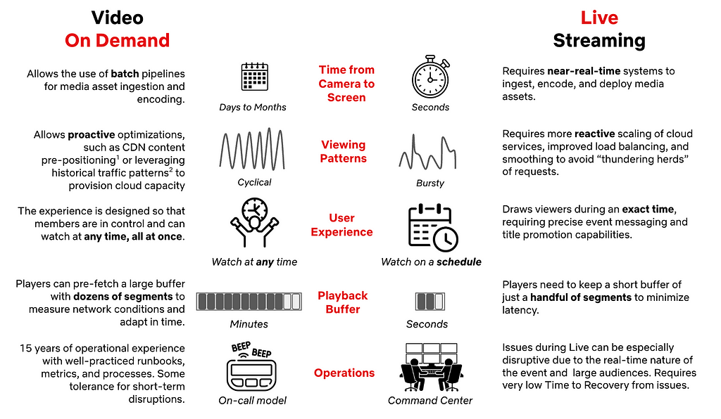
This means that we had a lot to build in order to make Live work well on Netflix. That starts with making the right choices regarding the fundamentals of our Live Architecture.
| Key Pillars of Netflix Live Architecture
Our Live Technology needed to extend the same promise to members that we’ve made with on-demand streaming: great quality on as many devices as possible without interruptions. Live is one of many entertainment formats on Netflix, so we also needed to seamlessly blend Live events into the user experience, all while scaling to over 300 million global subscribers.
When we started, we had nine months until the first launch. While we needed to execute quickly, we also wanted to architect for future growth in both magnitude and multitude of events. As a key principle, we leveraged our unique position of building support for a single product — Netflix — and having control over the full Live lifecycle, from Production to Screen.
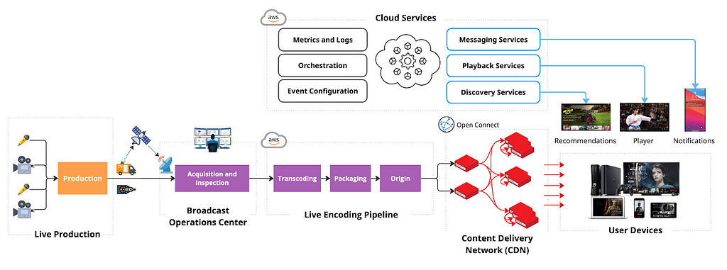
Dedicated Broadcast Facilities to Ingest Live Content from Production
Live events can happen anywhere in the world, but not every location has Live facilities or great connectivity. To ensure secure and reliable live signal transport, we leverage distributed and highly connected broadcast operations centers, with specialized equipment for signal ingest and inspection, closed-captioning, graphics and advertisement management. We prioritized repeatability, conditioning engineering to launch live events consistently, reliably, and cost-effectively, leaning into automation wherever possible. As a result, we have been able to reduce the event-specific setup to the transmission between production and the Broadcast Operations Center, reusing the rest across events.
Cloud-based Redundant Transcoding and Packaging Pipelines
The feed received at the Broadcast Center contains a fully produced program, but still needs to be encoded and packaged for streaming on devices. We chose a Cloud-based approach to allow for dynamic scaling, flexibility in configuration, and ease of integration with our Digital Rights Management (DRM), content management, and content delivery services already deployed in the cloud. We leverage AWS MediaConnect and AWS MediaLive to acquire feeds in the cloud and transcode them into various video quality levels with bitrates tailored per show. We built a custom packager to better integrate with our delivery and playback systems. We also built a custom Live Origin to ensure strict read and write SLAs for Live segments.
Scaling Live Content Delivery to millions of viewers with Open Connect CDN
In order for the produced media assets to be streamed, they need to be transferred from a few AWS locations, where Live Origin is deployed, to hundreds of millions of devices worldwide. We leverage Netflix’s CDN, Open Connect, to scale Live asset delivery. Open Connect servers are placed close to the viewers at over 6K locations and connected to AWS locations via a dedicated Open Connect Backbone network.
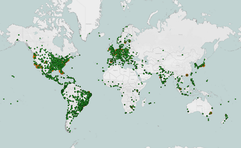
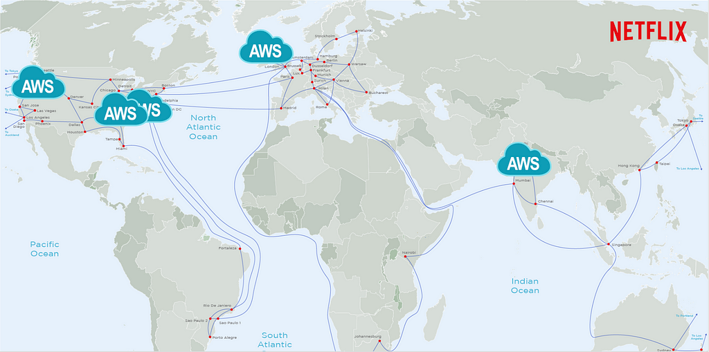
By enabling Live delivery on Open Connect, we build on top of $1B+ in Netflix investments over the last 12 years focused on scaling the network and optimizing the performance of delivery servers. By sharing capacity across on-demand and Live viewership we improve utilization, and by caching past Live content on the same servers used for on-demand streaming, we can easily enable catch-up viewing.
Optimizing Live Playback for Device Compatibility, Scale, Quality, and Stability
To make Live accessible to the majority of our customers without upgrading their streaming devices, we settled on using HTTPS-based Live Streaming. While UDP-based protocols can provide additional features like ultra-low latency, HTTPS has ubiquitous support among devices and compatibility with delivery and encoding systems. Furthermore, we use AVC and HEVC video codecs, transcode with multiple quality levels up from SD to 4K, and use a 2-second segment duration to balance compression efficiency, infrastructure load, and latency. While prioritizing streaming quality and playback stability, we have also achieved industry standard latency from camera to device, and continue to improve it.
To configure playback, the device player receives a playback manifest at the play start. The manifest contains items like the encoding bitrates and CDN servers players should use. We deliver the manifest from the cloud instead of the CDN, as it allows us to personalize the configuration for each device. To reference segments of the stream, the manifest includes a segment template that is used by devices to map a wall-clock time to URLs on the CDN. Using a segment template vs periodic polling for manifest updates minimizes network dependencies, CDN server load, and overhead on resource-constrained devices, like smart TVs, thus improving both scalability and stability of our system. While streaming, the player monitors network performance and dynamically chooses the bitrate and CDN server, maximizing streaming quality while minimizing rebuffering.
Run Discovery and Playback Control Services in the Cloud
So far, we have covered the streaming path from Camera to Device. To make the stream fully work, we also need to orchestrate across all systems, and ensure viewers can find and start the Live event. This functionality is performed by dozens of Cloud services, with functions like playback configuration, personalization, or metrics collection. These services tend to receive disproportionately higher loads around Live event start time, and Cloud deployment provides flexibility in dynamically scaling compute resources. Moreover, as Live demand tends to be localized, we are able to balance load across multiple AWS regions, better utilizing our global footprint. Deployment in the cloud also allows us to build a user experience where we embed Live content into a broader selection of entertainment options in the UI, like on-demand titles or Games.
Centralize Real-time Metrics in the Cloud with Specialized Tools and Facilities
With control over ingest, encoding pipelines, the Open Connect CDN, and device players, we have nearly end-to-end observability into the Live workflow. During Live, we collect system and user metrics in real-time (e.g., where members see the title on Netflix and their quality of experience), alerting us to poor user experiences or degraded system performance. Our real-time monitoring is built using a mix of internally developed tools, such as Atlas, Mantis, and Lumen, and open-source technologies, such as Kafka and Druid, processing up to 38 million events per second during some of our largest live events while providing critical metrics and operational insights in a matter of seconds. Furthermore, we set up dedicated “Control Center” facilities, which bring key metrics together to the operational team that monitors the event in real-time.
| Our key learnings so far
Building new functionality always brings fresh challenges and opportunities to learn, especially with a system as complex as Live. Even after three years, we’re still learning every day how to deliver Live events more effectively. Here are a few key highlights:
Extensive testing: Prior to Live we heavily relied on the predictable flow of on-demand traffic for pre-release canaries or A/B tests to validate deployments. But Live traffic was not always available, especially not at the scale representative of a big launch. As a result, we spent considerable effort to:
- Generate internal “test streams,” which engineers use to run integration, regression, or smoke tests as part of the development lifecycle.
- Build synthetic load testing capabilities to stress test cloud and CDN systems. We use 2 approaches, allowing us to generate up to 100K starts-per-second:
— Capture, modify, and replay past Live production traffic, representing a diversity of user devices and request patterns.
— Virtualize Netflix devices and generate traffic against CDN or Cloud endpoints to test the impact of the latest changes across all systems. - Run automated failure injection, forcing missing or corrupted segments from the encoding pipeline, loss of a cloud region, network drop, or server timeouts.
Regular practice: Despite rigorous pre-release testing, nothing beats a production environment, especially when operating at scale. We learned that having a regular schedule with diverse Live content is essential to making improvements while balancing the risks of member impact. We run A/B tests, perform chaos testing, operational exercises, and train operational teams for upcoming launches.
Viewership predictions: We use prediction-based techniques to pre-provision Cloud and CDN capacity, and share forecasts with our ISP and Cloud partners ahead of time so they can plan network and compute resources. Then we complement them with reactive scaling of cloud systems powering sign-up, log-in, title discovery, and playback services to account for viewership exceeding our predictions. We have found success with forward-looking real-time viewership predictions during a live event, allowing us to take steps to mitigate risks earlier, before more members are impacted.
Graceful degradation: Despite our best efforts, we can (and did!) find ourselves in a situation where viewership exceeded our predictions and provisioned capacity. In this case, we developed a number of levers to continue streaming, even if it means gradually removing some nice-to-have features. For example, we use service-level prioritized load shedding to prioritize live traffic over non-critical traffic (like pre-fetch). Beyond that, we can lighten the experience, like dialing down personalization, disabling bookmarks, or lowering the maximum streaming quality. Our load tests include scenarios where we under-scale systems to validate desired behavior.
Retry storms: When systems reach capacity, our key focus is to avoid cascading issues or further overloading systems with retries. Beyond system retries, users may retry manually — we’ve seen a 10x increase in traffic load due to stream restarts after viewing interruptions of as little as 30 seconds. We spent considerable time understanding device retry behavior in the presence of issues like network timeouts or missing segments. As a result, we implemented strategies like server-guided backoff for device retries, absorbing spikes via prioritized traffic shedding at Cloud Edge Gateway, and re-balancing traffic between cloud regions.
Contingency planning: “Everyone has a plan until they get punched in the mouth” is very relevant for Live. When something breaks, there is practically no time for troubleshooting. For large events, we set up in-person launch rooms with engineering owners of critical systems. For quick detection and response, we developed a small set of metrics as early indicators of issues, and have extensive runbooks for common operational issues. We don’t learn on launch day; instead, launch teams practice failure response via Game Day exercises ahead of time. Finally, our runbooks extend beyond engineering, covering escalation to executive leadership and coordination across functions like Customer Service, Production, Communications, or Social.
Our commitment to enhancing the member experience doesn’t end at the “Thanks for Watching!” screen. Shortly after each live stream, we dive into metrics to identify areas for improvement. Our Data & Insights team conducts comprehensive analyses, A/B tests, and consumer research to ensure the next event is even more delightful for our members. We leverage insights on member behavior, preferences, and expectations to refine the Netflix product experience and optimize our Live technology — like reducing latency by ~10 seconds through A/B tests, without affecting quality or stability.
| What’s next on our Live journey?
Despite three years of effort, we are far from done! In fact, we are just getting started, actively building on the learnings shared above to deliver more joy to our members with Live events. To support the growing number of Live titles and new formats, like FIFA WWC in 2027, we keep building our broadcast and delivery infrastructure and are actively working to further improve the Live experience.
In this post, we’ve provided a broad overview and have barely scratched the surface. In the upcoming posts, we will dive deeper into key pillars of our Live systems, covering our encoding, delivery, playback, and user experience investments in more detail.
Getting this far would not have been possible without the hard work of dozens of teams across Netflix, who collaborate closely to design, build, and operate Live systems: Operations and Reliability, Encoding Technologies, Content Delivery, Device Playback, Streaming Algorithms, UI Engineering, Search and Discovery, Messaging, Content Promotion and Distribution, Data Platform, Cloud Infrastructure, Tooling and Productivity, Program Management, Data Science & Engineering, Product Management, Globalization, Consumer Insights, Ads, Security, Payments, Live Production, Experience and Design, Product Marketing and Customer Service, amongst many others.

Behind the Streams: Live at Netflix. Part 1 was originally published in Netflix TechBlog on Medium, where people are continuing the conversation by highlighting and responding to this story.