Version
24.1 of the Arch-based Manjaro
distribution is now available with the 6.10 Linux kernel,
GNOME 46.5, KDE Plasma 6.1 and KDE Gear 24.08:
Plasma 6.1 on Wayland now has a feature that “remembers” what you were
doing in your last session like it did under X11. Although this is
still work in progress, If you log off and shut down your computer
with a dozen open windows, Plasma will now open them for you the next
time you power up your desktop, making it faster and easier to get
back to what you were doing. At Manjaro we are still defaulting to
X11, however switching to Wayland can be done easily by selecting the
wanted session in your display manager.
The project also offers minimal install images with the 6.6 LTS and
6.1 LTS kernels to support older hardware as needed.
Back in February, we celebrated our victory at trial in the U.S. District Court for the Western District of Texas against patent trolls Sable IP and Sable Networks. This was the culmination of nearly three years of litigation against Sable, but it wasn’t the end of the story.
Today we’re pleased to announce that the litigation against Sable has finally concluded on terms that we believe send a strong message to patent trolls everywhere — if you bring meritless patent claims against Cloudflare, we will fight back and we will win.
We’re also pleased to announce additional prizes in Project Jengo, and to make a final call for submissions before we determine the winners of the Final Awards. As a reminder, Project Jengo is Cloudflare’s effort to fight back against patent trolls by flipping the incentive structure that has encouraged the growth of patent trolls who extract settlements out of companies using frivolous lawsuits. We do this by asking the public to help identify prior art that can invalidate any of the patents that a troll holds, not just the ones that are asserted against Cloudflare. We’ve already given out over $125,000 to individuals since the launch of Project Jengo in 2017, and we’re looking forward to celebrating the successful end of the Sable iteration of Project Jengo with our Final Awards!
To learn more about how things concluded with Sable and next steps in Project Jengo, read on.
Background
For anyone just joining us on this odyssey, here is a little background on how we got here:
Sable sued Cloudflare back in March 2021. Sable is a patent troll. It doesn’t make, develop, innovate, or sell anything. Sable IP is merely a shell entity formed to monetize (make money from) an ancient patent portfolio acquired by Sable Networks from Caspian Networks in 2006. Caspian Networks was a router company that went out of business nearly 20 years ago. Using Caspian’s old patents, Sable sued Cloudflare and many other companies, including Cisco, Fortinet, Check Point, SonicWall, and Juniper Networks, alleging patent infringement. While these other companies resolved their disputes with Sable out of court, Cloudflare fought back.
Sable initially asserted around 100 claims from four different patents against Cloudflare, accusing multiple Cloudflare products and features of infringement. Sable’s patents — the old Caspian Networks patents — related to hardware-based router technologies common over 20 years ago. Sable’s infringement arguments stretched these patent claims to their limits (and beyond) as Sable tried to apply Caspian’s hardware-based technologies to Cloudflare’s modern software-defined services delivered on the cloud.
Cloudflare fought back against Sable by launching a new round of Project Jengo, Cloudflare’s prior art contest, seeking prior art to invalidate all of Sable’s patents.
After years of Cloudflare aggressively litigating against Sable’s patents before the U.S. Patent and Trademark Office and the district court, Sable was left with only one claim from one patent to assert against Cloudflare at trial. If you’d like to know more, we described those battles, in which Cloudflare successfully eliminated around 99% of Sable’s claims, in more detail in a prior blog post.
Sable and Cloudflare came together in a five-day jury trial in Waco, Texas in February 2024. At trial, Sable did its best to try to map its decades-old router technology onto Cloudflare’s modern software-based architecture. But Sable’s case was riddled with technical issues and its efforts backed only by the desire for a payout.
The jury agrees: Cloudflare does not infringe
To defeat Sable’s claim of infringement we needed to explain to the jury — in clear and understandable terms — why what Cloudflare does is different from what was covered by claim 25 of Sable’s remaining patent, U.S. Patent No. 7,012,919 (the ’919 patent). To do this, we enlisted the help of one of our talented Cloudflare engineers, Eric Reeves, as well as Dr. Paul Min, Senior Professor of Electrical & Systems Engineering at Washington University, an expert in the field of computer networking. Eric and Dr. Min helped us explain to the jury the multiple reasons we didn’t infringe.
From slide deck presented by Cloudflare to the jury during the trial
First, we explained that the accused Cloudflare products (Magic Transit and Argo for Packets) do not route “flows” or “micro-flows” as required by claim 25. Instead, they handle packets individually, on a packet-by-packet basis. Indeed, processing each packet individually is important to the functioning of these products and Cloudflare’s DDoS and security services as a whole.
Eric also helped to tell our invention story to the jury. He explained how the Cloudflare team saw problems that needed to be solved, and built unique and innovative new products to solve them. He described the work that went into developing Magic Transit and Argo for Packets, and how these products are part of Cloudflare’s modern software-based approach, which is fundamentally different from the hardware-based technology of the ’919 patent. Together, Eric and Dr. Min explained how the benefits of Magic Transit and Argo for Packets enjoyed by Cloudflare’s customers are not attributable to any technology claimed by the ’919 patent.
From slide deck presented by Cloudflare to the jury during the trial
Second, we explained that Cloudflare doesn’t infringe because claim 25 of the ’919 patent requires certain processes to occur “at” ingress and egress line cards, and Cloudflare’s accused servers do not include line cards.
From slide deck presented by Cloudflare to the jury during the trial
As Dr. Min explained, “line cards” are a specific type of hardware — a physical hardware “card” — that are commonly used in routers. Sable’s witnesses could not deny that the technology of the ’919 patent was tied to old router technology. After all, Caspian Networks Inc. (where the ’919 patent inventors worked) was a router company. Caspian’s core products were routers, and we showed the jury documents describing Caspian’s routers, which used “flow-based” technology on physical hardware line cards.
Trial exhibit, image of sample line card
While Sable’s technical expert tried his hardest to convince the jury that various software and hardware components of Cloudflare’s servers constitute “line cards,” his explanations defied credibility. The simple fact is that Cloudflare’s servers do not have line cards.
Ultimately, the jury understood, returning a verdict that Cloudflare does not infringe claim 25 of the ‘919 patent.
Excerpt from Verdict Form completed by the jury
The jury agrees: Sable’s patent claim is invalid
In addition to proving that we do not infringe, we also took on the challenge of proving to the jury that claim 25 of the ’919 patent is invalid and never should have been issued.
Proving invalidity to a jury is hard. The burden on the defendant is high: Cloudflare needed to prove by clear and convincing evidence that claim 25 is invalid. And, proving it by describing how the claim is obvious in light of the prior art is complicated.
To do this, we again relied on our technical expert, Dr. Min, to explain how two prior art references, U.S. Patent No. 6,584,071 (Kodialam) and U.S. Patent No. 6,680,933 (Cheeseman) together render claim 25 of the ’919 patent obvious. Kodialam and Cheeseman are patents from Nortel Networks and Lucent relating to router technology developed in the late 1990s. Both are prior art to the ’919 patent (i.e., they pre-date the priority date of the ’919 patent), and when considered together by a person skilled in the area of computer engineering and computer networking technology, they rendered obvious the so-called invention of claim 25.
Excerpt from Verdict Form completed by the jury
Sable does not get its payday …
Sable’s real motivation for suing Cloudflare — its desire for a payout — was made clear by Sable’s trial witnesses, who were unified only by their desire to present a wildly inflated view of the alleged “value” of the Sable patent and the damages allegedly owed by Cloudflare.
Sable’s attorneys tried their best to present their clients as reasonable businessmen, just trying to get what they’re owed for Cloudflare’s purported use of Sable’s patent. But Sable couldn’t hide its true colors from the jury. When Sable presented testimony from Brooks Borchers, the founder of Sable IP, Mr. Borchers was forced to admit that Sable IP is in the “business” of filing lawsuits.
Excerpt from Borchers trial testimony
In fact, Mr. Borchers was forced to admit that Sable’s approach is to sue first and ask questions later. Even among patent trolls, this is hardly a noble business practice.
Excerpts from Borchers trial testimony
What’s more, Mr. Borchers and his lawyers have teamed up on cases like this before, following the same sue-first-and-ask-questions-later playbook in hopes of a payout. Sable’s true motivations for suing Cloudflare were on full display after this testimony, making Sable’s damages demand all the more galling.
Sable’s damages expert, Stephen Dell, told the jury that Sable was owed somewhere between $25 million and $94.2 million in damages. But, Mr. Dell was forced to admit to multiple flaws in his damages calculation, and Cloudflare’s damages expert Chris Bakewell explained to the jury how bad inputs and faulty assumptions led Mr. Dell to a wildly inflated damages figure. Indeed, after hearing Sable’s expert’s testimony, Judge Albright said he was “very skeptical” of Mr. Dell’s opinions, explaining that he was “very concerned that there’s not support for his methodology.”
In the end, Mr. Dell’s outsized damages demand didn’t matter because the jury found that Cloudflare did not infringe and that the asserted patent claim is invalid. But, it was revealing of Sable’s motivation (greed) and the lengths that it would go to try to get a payout.
When all was said and done, after all the testimony and argument, we were thrilled when the jury returned its verdict — after less than two hours of deliberations — finding across the board for Cloudflare. The jury’s verdict is truly a validation of our strong belief in the importance of standing up to patent trolls like Sable, and we are grateful for the jury’s time, attention and consideration!
Sable admits defeat, and agrees to pay Cloudflare!
A jury verdict is not the end of the road in a patent case … there are post-trial motions, appeals, and other procedural hurdles to jump through before a case is truly over. Tired from the fight, and smarting from its loss, Sable decided it wanted to throw in the towel and end the fight once and for all.
In the end, Sable agreed to pay Cloudflare $225,000, grant Cloudflare a royalty-free license to its entire patent portfolio, and to dedicate its patents to the public, ensuring that Sable can never again assert them against another company.
Let’s repeat that first part, just to make sure everyone understands:
Sable, the patent troll that sued Cloudflare back in March 2021 asserting around 100 claims across four patents, in the end wound up paying Cloudflare. While this $225,000 can’t fully compensate us for the time, energy and frustration of having to deal with this litigation for nearly three years, it does help to even the score a bit. And we hope that it sends an important message to patent trolls everywhere to beware before taking on Cloudflare.
Excerpt from the Dedication to the Public and Royalty Free License Agreement between Sable and Cloudflare
And, let’s talk a bit more about that final part:
Sable has agreed to dedicate its entire patent portfolio to the public. This means that Sable will tell the U.S. Patent and Trademark Office that it gives up all of its legal rights to its patent portfolio. Sable can never again use these patents to sue for infringement; they can never again use these patents to try to make a quick buck.
Excerpt from the Dedication to the Public and Royalty Free License Agreement between Sable and Cloudflare
To sum it up …
Cloudflare fought back against the patent troll and we won. We not only defeated Sable’s claims in court, we forced Sable to pay Cloudflare for the trouble, and we got Sable’s patents dedicated to the public, ensuring that it can never assert these patents against any other company ever again. It was admittedly a lot of work for Cloudflare, but totally worth it.
Project Jengo for Sable: Conclusion of the Case
A crucial part of our efforts to secure this across-the-board win are our Project Jengo participants.
Since the launch of the Project Jengo for the Sable case, we’ve received hundreds of prior art references from dedicated Project Jengo participants. So far we have awarded $70,000 in prizes to the winners of Chapters 1 through 8. And we still have $30,000 in prizes to award in the Final Awards.
This blog post marks the official “Conclusion of the Case” under the Project Jengo Sable Rules. We will continue to accept submissions during the 30-day Grace Period, which lasts until November 2, 2024, and then will move on to selecting winners of the Final Awards.
We are thrilled to announce the winners of Chapters 7 and 8
We publicly celebrated the Chapter 1, Chapter 2, Chapter 3 and Chapters 4-6 winners in previous blog posts. However, as the trial approached in the Sable case, we chose not to make public announcements for the Chapter 7 and 8 winners out of respect for the judicial process. Now that the case is over, we are delighted to give a big public shout out to the winners of Project Jengo Chapters 7 and 8!
We selected four total winners in Chapters 7 and 8, each receiving prizes of $5,000, for a grand total of $20,000. Our Chapter 7 winners, George W. and Madhu, each provided helpful and detailed charts containing element-by-element comparisons of the prior art to the relevant Sable patents. George W. is an electrical engineer and lawyer, who is active in the intellectual property community. He learned about Project Jengo in an article posted online, and thought it was a clever idea. The Chapter 8 winners, Jatin and Ketan, also provided thoughtful and detailed submissions. Jatin submitted two pieces of prior art that were particularly good references for Sable’s U.S. Patent No. 7,012,919, which contains the one claim that remained asserted against Cloudflare at trial.
We also want to again thank our prior chapter winners and everyone who participated in Project Jengo! We look forward to selecting the Final Awards winners — it will be fun to take a walk down memory lane re-reviewing the fantastic prior art submitted by our prior winners, and we can’t wait to check out the new submissions, too! Please use the “Submit Prior Art” link on this page for your final entries. Once we’ve announced our Final Awards, we will also update the Sable patents prior art listing on our website, to share all the prior art submitted by our Project Jengo participants.
Since early September, Cloudflare’s DDoS protection systems have been combating a month-long campaign of hyper-volumetric L3/4 DDoS attacks. Cloudflare’s defenses mitigated over one hundred hyper-volumetric L3/4 DDoS attacks throughout the month, with many exceeding 2 billion packets per second (Bpps) and 3 terabits per second (Tbps). The largest attack peaked 3.8 Tbps — the largest ever disclosed publicly by any organization. Detection and mitigation was fully autonomous. The graphs below represent two separate attack events that targeted the same Cloudflare customer and were mitigated autonomously.
A mitigated 3.8 Terabits per second DDoS attack that lasted 65 seconds
A mitigated 2.14 billion packet per second DDoS attack that lasted 60 seconds
Cloudflare customers are protected
Cloudflare customers using Cloudflare’s HTTP reverse proxy services (e.g. Cloudflare WAF and Cloudflare CDN) are automatically protected.
Cloudflare customers using Spectrum and Magic Transit are also automatically protected. Magic Transit customers can further optimize their protection by deploying Magic Firewall rules to enforce a strict positive and negative security model at the packet layer.
Other Internet properties may not be safe
The scale and frequency of these attacks are unprecedented. Due to their sheer size and bits/packets per second rates, these attacks have the ability to take down unprotected Internet properties, as well as Internet properties that are protected by on-premise equipment or by cloud providers that just don’t have sufficient network capacity or global coverage to be able to handle these volumes alongside legitimate traffic without impacting performance.
Cloudflare, however, does have the network capacity, global coverage, and intelligent systems needed to absorb and automatically mitigate these monstrous attacks.
In this blog post, we will review the attack campaign and why its attacks are so severe. We will describe the anatomy of a Layer 3/4 DDoS attack, its objectives, and how attacks are generated. We will then proceed to detail how Cloudflare’s systems were able to autonomously detect and mitigate these monstrous attacks without impacting performance for our customers. We will describe the key aspects of our defenses, starting with how our systems generate real-time (dynamic) signatures to match the attack traffic all the way to how we leverage kernel features to drop packets at wire-speed.
Campaign analysis
We have observed this attack campaign targeting multiple customers in the financial services, Internet, and telecommunication industries, among others. This attack campaign targets bandwidth saturation as well as resource exhaustion of in-line applications and devices.
The attacks predominantly leverage UDP on a fixed port, and originated from across the globe with larger shares coming from Vietnam, Russia, Brazil, Spain, and the US.
The high packet rate attacks appear to originate from multiple types of compromised devices, including MikroTik devices, DVRs, and Web servers, orchestrated to work in tandem and flood the target with exceptionally large volumes of traffic. The high bitrate attacks appear to originate from a large number of compromised ASUS home routers, likely exploited using a CVE 9.8 (Critical) vulnerability that was recently discovered by Censys.
Anatomy of DDoS attacks
Before we discuss how Cloudflare automatically detected and mitigated the largest DDoS attacks ever seen, it‘s important to understand the basics of DDoS attacks.
Simplified diagram of a DDoS attack
The goal of a Distributed Denial of Service (DDoS) attack is to deny legitimate users access to a service. This is usually done by exhausting resources needed to provide the service. In the context of these recent Layer 3/4 DDoS attacks, that resource is CPU cycles and network bandwidth.
Exhausting CPU cycles
Processing a packet consumes CPU cycles. In the case of regular (non-attack) traffic, a legitimate packet received by a service will cause that service to perform some action, and different actions require different amounts of CPU processing. However, before a packet is even delivered to a service there is per-packet work that needs to be done. Layer 3 packet headers need to be parsed and processed to deliver the packet to the correct machine and interface. Layer 4 packet headers need to be processed and routed to the correct socket (if any). There may be multiple additional processing steps that inspect every packet. Therefore, if an attacker sends at a high enough packet rate, then they can potentially saturate the available CPU resources, denying service to legitimate users.
To defend against high packet rate attacks, you need to be able to inspect and discard the bad packets using as few CPU cycles as possible, leaving enough CPU to process the good packets. You can additionally acquire more, or faster, CPUs to perform the processing — but that can be a very lengthy process that bears high costs.
Exhausting network bandwidth
Network bandwidth is the total amount of data per time that can be delivered to a server. You can think of bandwidth like a pipe to transport water. The amount of water we can deliver through a drinking straw is less than what we could deliver through a garden hose. If an attacker is able to push more garbage data into the pipe than it can deliver, then both the bad data and the good data will be discarded upstream, at the entrance to the pipe, and the DDoS is therefore successful.
Defending against attacks that can saturate network bandwidth can be difficult because there is very little that can be done if you are on the downstream side of the saturated pipe. There are really only a few choices: you can get a bigger pipe, you can potentially find a way to move the good traffic to a new pipe that isn’t saturated, or you can hopefully ask the upstream side of the pipe to stop sending some or all of the data into the pipe.
Generating DDoS attacks
If we think about what this means from the attackers point of view you realize there are similar constraints. Just as it takes CPU cycles to receive a packet, it also takes CPU cycles to create a packet. If, for example, the cost to send and receive a packet were equal, then the attacker would need an equal amount of CPU power to generate the attack as we would need to defend against it. In most cases this is not true — there is a cost asymmetry, as the attacker is able to generate packets using fewer CPU cycles than it takes to receive those packets. However, it is worth noting that generating attacks is not free and can require a large amount of CPU power.
Saturating network bandwidth can be even more difficult for an attacker. Here the attacker needs to be able to output more bandwidth than the target service has allocated. They actually need to be able to exceed the capacity of the receiving service. This is so difficult that the most common way to achieve a network bandwidth attack is to use a reflection/amplification attack method, for example a DNS Amplification attack. These attacks allow the attacker to send a small packet to an intermediate service, and the intermediate service will send a large packet to the victim.
In both scenarios, the attacker needs to acquire or gain access to many devices to generate the attack. These devices can be acquired in a number of different ways. They may be server class machines from cloud providers or hosting services, or they can be compromised devices like DVRs, routers, and webcams that have been infected with the attacker’s malware. These machines together form the botnet.
How Cloudflare defends against large attacks
Now that we understand the fundamentals of how DDoS attacks work, we can explain how Cloudflare can defend against these attacks.
Spreading the attack surface using global anycast
The first not-so-secret ingredient is that Cloudflare’s network is built on anycast. In brief, anycast allows a single IP address to be advertised by multiple machines around the world. A packet sent to that IP address will be served by the closest machine. This means when an attacker uses their distributed botnet to launch an attack, the attack will be received in a distributed manner across the Cloudflare network. An infected DVR in Dallas, Texas will send packets to a Cloudflare server in Dallas. An infected webcam in London will send packets to a Cloudflare server in London.
Anycast vs. Unicast networks
Our anycast network additionally allows Cloudflare to allocate compute and bandwidth resources closest to the regions that need them the most. Densely populated regions will generate larger amounts of legitimate traffic, and the data centers placed in those regions will have more bandwidth and CPU resources to meet those needs. Sparsely populated regions will naturally generate less legitimate traffic, so Cloudflare data centers in those regions can be sized appropriately. Since attack traffic is mainly coming from compromised devices, those devices will tend to be distributed in a manner that matches normal traffic flows sending the attack traffic proportionally to datacenters that can handle it. And similarly, within the datacenter, traffic is distributed across multiple machines.
Additionally, for high bandwidth attacks, Cloudflare’s network has another advantage. A large proportion of traffic on the Cloudflare network does not consume bandwidth in a symmetrical manner. For example, an HTTP request to get a webpage from a site behind Cloudflare will be a relatively small incoming packet, but produce a larger amount of outgoing traffic back to the client. This means that the Cloudflare network tends to egress far more legitimate traffic than we receive. However, the network links and bandwidth allocated are symmetrical, meaning there is an abundance of ingress bandwidth available to receive volumetric attack traffic.
Generating real-time signatures
By the time you’ve reached an individual server inside a datacenter, the bandwidth of the attack has been distributed enough that none of the upstream links are saturated. That doesn’t mean the attack has been fully stopped yet, since we haven’t dropped the bad packets. To do that, we need to sample traffic, qualify an attack, and create rules to block the bad packets.
Sampling traffic and dropping bad packets is the job of our l4drop component, which uses XDP (eXpress Data Path) and leverages an extended version of the Berkeley Packet Filter known as eBPF (extended BPF). This enables us to execute custom code in kernel space and process (drop, forward, or modify) each packet directly at the network interface card (NIC) level. This component helps the system drop packets efficiently without consuming excessive CPU resources on the machine.
Cloudflare DDoS protection system overview
We use XDP to sample packets to look for suspicious attributes that indicate an attack. The samples include fields such as the source IP, source port, destination IP, destination port, protocol, TCP flags, sequence number, options, packet rate and more. This analysis is conducted by the denial of service daemon (dosd).Dosd holds our secret sauce. It has many filters which instruct it, based on our curated heuristics, when to initiate mitigation. To our customers, these filters are logically grouped by attack vectors and exposed as the DDoS Managed Rules. Our customers can customize their behavior to some extent, as needed.
As it receives samples from XDP, dosd will generate multiple permutations of fingerprints for suspicious traffic patterns. Then, using a data streaming algorithm, dosd will identify the most optimal fingerprints to mitigate the attack. Once attack is qualified, dosd will push a mitigation rule inline as an eBPF program to surgically drop the attack traffic.
The detection and mitigation of attacks by dosd is done at the server level, at the data center level and at the global level — and it’s all software defined. This makes our network extremely resilient and leads to almost instant mitigation. There are no out-of-path “scrubbing centers” or “scrubbing devices”. Instead, each server runs the full stack of the Cloudflare product suite including the DDoS detection and mitigation component. And it is all done autonomously. Each server also gossips (multicasts) mitigation instructions within a data center between servers, and globally between data centers. This ensures that whether an attack is localized or globally distributed, dosd will have already installed mitigation rules inline to ensure a robust mitigation.
Strong defenses against strong attacks
Our software-defined, autonomous DDoS detection and mitigation systems run across our entire network. In this post we focused mainly on our dynamic fingerprinting capabilities, but our arsenal of defense systems is much larger. The Advanced TCP Protection system and Advanced DNS Protection system work alongside our dynamic fingerprinting to identify sophisticated and highly randomized TCP-based DDoS attacks and also leverages statistical analysis to thwart complex DNS-based DDoS attacks. Our defenses also incorporate real-time threat intelligence, traffic profiling, and machine learning classification as part of our Adaptive DDoS Protection to mitigate traffic anomalies.
Together, these systems, alongside the full breadth of the Cloudflare Security portfolio, are built atop of the Cloudflare network — one of the largest networks in the world — to ensure our customers are protected from the largest attacks in the world.
В последната седмица от съществуването си парламентът почти без дебати върна гражданските права на голяма група хора. Това стана с подкрепата на ГЕРБ и ПП–ДБ и въпреки всички останали парламентарни групи (плюс независимите депутати). Инициативата е на трима депутати – Деница Сачева (ГЕРБ), Божидар Божанов (ПП–ДБ, „Да, България“) и Александър Ненков (ГЕРБ).
Става въпрос за промените в Закона за гражданската регистрация (ЗГР), с които се въвежда т.нар. служебен адрес. На такъв могат да бъдат регистрирани хората, които по една или друга причина не са в състояние да докажат редовен постоянен адрес в България. А без това не могат да им се издадат документи за самоличност.
Какво не можем без лични документи?
Замисляли ли сте се за колко много неща, които смятаме за даденост, ни трябват документи за самоличност? Без лична карта или паспорт не можем не само да гласуваме или да сключим брак. Нямаме право и да се осигуряваме, да имаме законен дом, все едно дали собствен, или под наем, банкова сметка. Не можем да пътуваме в чужбина, да сключваме договори, не можем дори да имаме телефон на свое име.
Строго погледнато, дори на улицата не можем да излезем, защото, ако служител на реда поиска да се легитимираме, сме длъжни да представим личен документ. Нито можем да заведем съдебно дело, че са нарушени правата ни.
Ромският активист Огнян Исаев дава още примери какво означава да нямаш лична карта:
Парче пластика, а всъщност свобода или робство… да не можеш да припознаеш новороденото си дете, да не можеш да запишеш детето си на градина или училище, да не можеш да работиш и да имаш доходи, да не можеш да се разболяваш, защото няма как да се лекуваш… да не можеш дори да напуснеш този ад, в който си се озовал.
Изглежда абсурдно, но ако нямате лични документи, могат да откажат дори да ви погребат. На това основание през 2009 г. българските власти в продължение на две седмици са отказвали погребение на нигерийския протестантски пастор Джонсън Ибитуй, разказва синът му. Ибитуй е преподавал в български университет, имал е езикова школа, но когато не успял да поднови документите си, държавата го сметнала за недостоен и за вечен покой.
Колко и какви са хората без български документи за самоличност?
Оценките за броя на българските граждани и чужденците в България, които не могат да се регистрират по постоянен адрес в страната и поради това остават без документи за самоличност, варират в много широки граници. Според „Продължаваме промяната“ българските граждани с този проблем са над 50 000.
В годишния доклад на Българския хелзинкски комитет (БХК) за 2022 г. обаче се посочва, че към юли 2022 г. 187 883 български граждани нямат лична карта, като 109 233 от тях живеят в България и имат настоящ адрес (но за издаване на документи за самоличност е нужен постоянен адрес). От БХК са получили данните от МВР по реда на Закона за достъп до обществена информация, но от Вътрешното министерство са отказали да предоставят сведения колко точно са хората с „невалиден“ адрес.
При всички случаи мнозинството неможещи да се регистрират адресно в България са български граждани. Те се делят на две основни групи. В първата влизат предимно хора от ромски махали. Някои от тях например живеят в къщи, които никога не са били узаконявани, и затова нямат валиден адрес. Обитателите на много от тези къщи нямат и договори с дружествата, предоставящи комунални услуги. Други са имали адресна регистрация, но са принудително изведени от домовете си, за да бъдат жилищата им съборени. После адресът е заличен и хората не могат да се регистрират отново.
Втората голяма група са българите в чужбина, които не притежават имот в България. За да се регистрира адресно, човек трябва да представи нотариален акт, договор за наем (с писмено съгласие от наемодателя) или доказателство за платени битови сметки. При липса на такива не се издават лични документи. Затова много от тези хора, макар формално да не са лишени от българското си гражданство, на практика губят своите граждански права в родината си. А ако нямат двойно гражданство, липсата на български документи създава проблем за статута им и в страните, в които пребивават.
В България има, макар и далеч по-малко, чужденци, които не могат да си извадят документи за самоличност. Сред тях са чужденците без легален статут, но не само те. Някои от хората, получили статут на бежанци, хуманитарен статут или убежище в България, научавайки добрата новина, че страната е решила да ги спаси, изпадат в омагьосан кръг. Те са живели в някое от общежитията на Държавната агенция за бежанците и след получаването на статута са длъжни да устроят живота си сами. Трябва бързо да си извадят лични документи, но за тази цел се налага да имат адресна регистрация. Няма как обаче да се сдобият с договор за наем, ако нямат лични документи.
Как се стигна до омагьосания кръг с адресните регистрации и документите за самоличност?
През 2011 г. на власт е първото правителство на Бойко Борисов. От ГЕРБ внасят подписан лично от Борисов законопроект за промяна на ЗГР. С него се предлага за адресна регистрация да се представя документ за собственост или за право на ползване, както и съгласие от собственика – или лично, или нотариално заверено. Предвижда се и хората, променили настоящия си адрес между 01.09.2010 г. и 31.01.2011 г., да се регистрират отново.
Краят на януари 2011 г. е избран във връзка с промените в Изборния кодекс, с които се въвежда т.нар. уседналост при гласуването – задължението едно лице да е било регистрирано по постоянен или настоящ адрес определен брой месеци преди изборите.
В проекта за промяна на ЗГР се посочва като мотив защитата на интересите на собствениците срещу случаи на злоупотреби – на адреса на имота им се регистрират хора, които не живеят на него. По-важната цел обаче е борбата с т.нар. изборен туризъм – практиката избиратели да се регистрират в определена община само за да гласуват в нея.
Законопроектът е приет на второ четене в парламента почти без дебати, като се изключи точката за пререгистрирането на променилите адреса си между 01.09.2010 г. и 31.01.2011 г. Възразяват от БСП, а особено активна е Мая Манолова, която смята предложението за противоконституционно. Според нея „минимум 50 000 български граждани ще бъдат наказани“ в резултат на това изискване, защото ще трябва да повторят едно административно действие, представяйки документи, които не са им били нужни преди.
Въпреки че в началото на парламентарното заседание се регистрират 124 депутати, по-малко от 80 участват в гласуването на промените в ЗГР, като повечето са от ГЕРБ, а народните представители от останалите групи масово не се включват. Единствено по точката, срещу която възразява Манолова, 9 депутати от БСП гласуват против.
В дебатите не се засяга темата, че промените ще доведат до лишаването на десетки хиляди български граждани от граждански права, тъй като ще ги оставят без документи за самоличност.
През декември 2011 г. обаче Мая Манолова и съпартийката ѝ Милена Христова внасят законопроект за облекчаване на правилата за адресната регистрация. „Без лична карта един човек е анонимен и напълно безпомощен“, аргументира се Манолова. Според нея в резултат на затягането на правилата за адресна регистрация около 10 000 души остават без лични документи, „но процесът е лавинообразен и ще засяга все повече хора“.
В резултат правилата леко се облекчават, като се добавят и други документи, с които човек да доказва, че живее на определен адрес – например битови сметки. Но това не решава проблема на голямата част от хората, които остават без български документи за самоличност – въпреки всички анализи и доклади (ето например един от първите) за огромните измерения на проблема.
Освен ромите и българите в чужбина, потърпевши от промените в ЗГР през 2011 г., макар и в по-малка степен, са и част от хората, които живеят под наем в България. Причината е, че доста хазяи отказват да съдействат за адресната регистрация на наемателите, за да не им се наложи да плащат данъци върху наемите. Това затруднява наемателите да гласуват, ако трябва да пътуват с часове до постоянния си адрес. Също не могат да имат личен лекар в населеното място, в което живеят, нито децата им имат шанс в класациите за детска градина и основно училище.
Как се стигна до въвеждането на служебни адреси?
Седмица преди приемането на последните промени в ЗГР, с които се въведоха служебните адреси, от ПП се похвалиха, че идеята е тяхна и на коалиционните им партньори от „Демократична България“ (ДБ). И подчертаха, че инициативата е още от времето на кабинета на Кирил Петков, когато е създадена работна група към Министерството на регионалното развитие и благоустройството (МРРБ) по темата. А законопроектът е довършен по времето на правителството на Николай Денков.
Вярно е, че през януари 2024 г., когато премиер беше Денков, МРРБ анонсира въвеждането на служебен адрес за гражданите без редовен адрес. ПП обаче не са сред вносителите на последните предложения, които бяха приети на 25 септември 2024 г. и които са внесени от Деница Сачева и Александър Ненков от ГЕРБ и Божидар Божанов от „Да, България“, част от ДБ.
Освен това нито ПП, нито ДБ, нито впрочем и ГЕРБ са внесли законопроект за промяна на ЗГР. Сачева, Божанов и Ненков всъщност внасят в Комисията по регионална политика доклад с предложение за допълване на законопроект на „Възраждане“.
От партията на Костадин Костадинов предлагат ЗГР да стане още по-рестриктивен за хората с проблеми с адресната регистрация. Те искат да има проверки по домовете, за да се установи дали регистриралите се на един адрес действително живеят там, а също така да се увеличат санкциите за нарушителите. А това би засегнало онези, които са помогнали на хора, неможещи да докажат редовен адрес, като са им предоставили своя. Особено засегнати са и гражданите, които няма да могат вече да разчитат на такава помощ и има вероятност да останат без документи за самоличност заради това.
Предложенията, внесени от Сачева, Божанов и Ненков, представляват решение на проблема с невъзможните адресни регистрации на ромите, попаднали в омагьосания кръг на отнетите граждански права, на българите в чужбина, които не разполагат с имот в родината си, както и на бежанците, получили легален статут.
Гласуването протича с доста рехаво участие от страна на част от парламентарните групи. Най-стабилно присъствие имат от ГЕРБ, ПП–ДБ, „Възраждане“ и ИТН. От ДПС се включват максимум 10 депутати, от БСП – 4, от независимите – 7. Самото гласуване е разделено на 16 части, защото предложените текстове са много. В повечето случаи ГЕРБ и ПП–ДБ гласуват заедно, а срещу тях са „Възраждане“, ИТН и депутатите от останалите групи. Тоест от ДПС гласуват срещу правата на част от традиционните си избиратели, а БСП вече не се и опитва да е социална както през 2011 г., а е последователно националпопулистка.
Дебати почти няма. Срещу въвеждането на служебни адреси възразява депутатката от „Възраждане“ Маргарита Махаева. „За вечни времена ли ще бъде тази регистрация?“, пита тя. Според нея служебните адреси трябва да се предоставят „само в изключителни случаи“ и за кратък период. „След това да намерят къде да се регистрират, вече е тяхна си работа“, смята Махаева. Контрапредложенията ѝ не се приемат.
Служебните адреси помагат за възстановяването на правата на хората в гетата и на емигрантите, но нямат отношение към проблемите на наемателите, чиито хазяи отказват да ги регистрират, защото укриват данъци.
„Глътка въздух“ – позицията на ромския активист
Огнян Исаев разглежда промените в ЗГР в контекста на правата на ромите. В коментар за „Тоест“ той припомня, че „още от създаването на Третата българска държава българските власти някъде частично, някъде изцяло ограничават гражданските права на ромите“. Например през 1901 г. Народното събрание отнема избирателните им права. Според Исаев промените в ЗГР от 2011 г. на практика отнемат гражданството на голям брой роми.
Много български политици си мислят, че ромските избиратели се печелят само с купуване и натиск, а не „с нормални и човешки разговори“, смята Исаев. Той определя последните промени в ЗГР като „глътка въздух“. Но подчертава, че „истинското освобождение ще настъпи, когато се промени и Законът за устройство на територията така, че всички неформални ромски махали станат формално част от общините, а не бели петна на картите им“.
„Ромските тегоби са експериментални“, казва Огнян Исаев и пояснява: ако експериментите с ограничаването на правата на ромите са успешни, те ще се приложат под една или друга форма върху цялото население.
Същото твърдение се отнася и за ЛГБТИ (лесбийки, гей мъже, бисексуални, транс и интерсекс) хората, както и за всяка друга група, обявена за „обществен враг“. Когато се приеха поправките по руски образец против ЛГБТИ „пропагандата“ в училище в Закона за училищното и предучилищното образование, вносителите от „Възраждане“ веднага пробваха да прокарат и регистрацията на т.нар. чуждестранни агенти – отново в унисон с путинското законодателство. Предложението не мина най-вече защото от ГЕРБ бяха против. Както впрочем и промените в ЗГР през 2011 и през 2024 г., и забраната на „пропагандата“ в училище минаха, защото ГЕРБ беше за.
Обратите в отнемането и предоставянето на права показват как в българската политика базови ценности се превръщат в залог на ситуативни интереси и моментни конфигурации. Така човек не знае дали утре ще го превърнат в поредната опитна мишка с отнети права, или ще го прехвърлят от групата на мишките при човешките същества. Днес поне за ромите има „глътка въздух“. До следващата изненада.
„8. Намаляване на бюрокрацията във връзка превенцията на прането на пари – повече служебни справки и по-малко излишни документи, които финансовите институции и други организации събират от клиентите си.“
Почти всеки клиент на банка е бил викан да си даде актуални данни. Искат се всякакви документи – и фирмени, и лични. И всичко това, за да се изпълнят криворазбраните изисквания за превенция на пране на пари. Защо криворазбрани – защото при цялата бюрокрация, България има сериозен проблем с прането на пари, влезе в сивия списък на рискови държави, а напр.
Божков изтегли необезпокояван 67 милиона в кеш.
Междувременно, Европейският съюз прие шестия пакет мерки срещу изпирането на пари, което значи още промени в близко бъдеще. България спазва „буквата“ на закона, но често ѝ убягва духа, което значи прекомерна тежест без нужния ефект.
В 49-ото Народно събрание свърших две неща по темата: 1) събрах (с помощта на бранша) конкретни справки в публични регистри, които, ако бъдат приложени, могат да спестят разнасяне на документи, свързани с изпирането на пари, и 2) прокарах облекчения в Закона за мерките срещу изпирането на пари, така че да не отпадне задължението за представяне на документи, които могат да бъдат свалени от Търговския регистър. С моя редакция беше уредено и съхранението и достъпа до електронен архив (когато оригиналните документи са електронни).
В следващия парламент ще опитам да придвижа отпадането на максимално голямо количество излишни документи, които могат да бъдат заменени със справки; което пък ще спести фразата „обикалям за едни документи“ и периодичното разхождане до клон на финансови институции.
Смятам също така, че финансовото разузнаване, което е основен орган за превенцията на пране на пари, трябва да бъде в структурата на Министерство на финансите, защото в ДАНС няма добра среда за съвременни методи за превенция.
С по-малко бюрокрация и повече ефективност и дигитализация можем едновременно да облекчим финансовите институции, гражданите и бизнеса, и да постигнем по-добри резултати в борбата с прането на пари.
Amazon Redshift enables you to efficiently query and retrieve structured and semi-structured data from open format files in Amazon S3 data lake without having to load the data into Amazon Redshift tables. Amazon Redshift extends SQL capabilities to your data lake, enabling you to run analytical queries. Amazon Redshift supports a wide variety of tabular data formats like CSV, JSON, Parquet, ORC and open tabular formats like Apache Hudi, Linux foundation Delta Lake and Apache Iceberg.
You create Redshift external tables by defining the structure for your files, S3 location of the files and registering them as tables in an external data catalog. The external data catalog can be AWS Glue Data Catalog, the data catalog that comes with Amazon Athena, or your own Apache Hive metastore.
Over the last year, Amazon Redshift added several performance optimizations for data lake queries across multiple areas of query engine such as rewrite, planning, scan execution and consuming AWS Glue Data Catalog column statistics. To get the best performance on data lake queries with Redshift, you can use AWS Glue Data Catalog’s column statistics feature to collect statistics on Data Lake tables. For Amazon Redshift Serverless instances, you will see improved scan performance through increased parallel processing of S3 files and this happens automatically based on RPUs used.
In this post, we highlight the performance improvements we observed using industry standard TPC-DS benchmarks. Overall execution time of TPC-DS 3 TB benchmark improved by 3x. Some of the queries in our benchmark experienced up to 12x speed up.
Performance Improvements
Several performance optimizations were done over the last year to improve performance of data lake queries including the following.
Consume AWS Glue Data Catalog column statistics and tuning of Redshift optimizer to improve quality of query plans
Utilize bloom filters for partition columns
Improved scan efficiency for Amazon Redshift Serverless instances through increased parallel processing of files
Novel query rewrite rules to merge similar scans
Faster retrieval of metadata from AWS Glue Data Catalog
To understand the performance gains, we tested the performance on the industry-standard TPC-DS benchmark using 3 TB data sets and queries which represents different customer use cases. Performance was tested on a Redshift serverless data warehouse with 128 RPU. In our testing, the dataset was stored in Amazon S3 in Parquet format and AWS Glue Data Catalog was used to manage external databases and tables. Fact tables were partitioned on the date column, and each fact table consisted of approximately 2,000 partitions. All of the tables had their row count table property, numRows, set as per the spectrum query performance guidelines.
We did a baseline run on Redshift patch version (patch 172) from last year. Later, we ran all TPC-DS queries on latest patch version (patch 180) that includes all performance optimizations added over last year. Then we used AWS Glue Data Catalog’s column statistics feature to compute statistics for all the tables and measured improvements with the presence of AWS Glue Data Catalog column statistics.
Our analysis revealed that the TPC-DS 3TB Parquet benchmark saw substantial performance gains with these optimizations. Specifically, partitioned Parquet with our latest optimizations achieved 2x faster runtimes compared to the previous implementation. Enabling AWS Glue Data Catalog column statistics further improved performance by 3x versus last year. The following graph illustrates these runtime improvements for the full benchmark (all TPC-DS queries) over the past year, including the additional boost from using AWS Glue Data Catalog column statistics.
Figure 1: Improvement in total runtime of TPC-DS 3T workload
The following graph presents the top queries from the TPC-DS benchmark with the greatest performance improvement over the last year with and without AWS Glue Data Catalog column statistics. You can see that performance improves a lot when statistics exist on AWS Glue Data Catalog (for details on how to get statistics for your Data Lake tables, please refer to optimizing query performance using AWS Glue Data Catalog column statistics). Specifically, multi-join queries will benefit the most from AWS Glue Data Catalog column statistics because the optimizer uses statistics to choose the right join order and distribution strategy.
Figure 2: Speed-up in TPC-DS queries
Let’s discuss some of the optimizations that contributed to improved query performance.
Optimizing with table-level statistics
Amazon Redshift’s design enables it to handle large-scale data challenges with superior speed and cost-efficiency. Its massively parallel processing (MPP) query engine, AI-powered query optimizer, auto-scaling capabilities, and other advanced features allow Redshift to excel at searching, aggregating, and transforming petabytes of data.
However, even the most powerful systems can experience performance degradation if they encounter anti-patterns like grossly inaccurate table statistics, such as the row count metadata.
Without this crucial metadata, Redshift’s query optimizer may be limited in the number of possible optimizations, especially those related to data distribution during query execution. This can have a significant impact on overall query performance.
To illustrate this, consider the following simple query involving an inner join between a large table with billions of rows and a small table with only a few hundred thousand rows.
select small_table.sellerid, sum(large_table.qtysold)
from large_table, small_table
where large_table.salesid = small_table.listid
 and small_table.listtime > '2023-12-01'
 and large_table.saletime > '2023-12-01'
group by 1 order by 1
If executed as-is, with the large table on the right-hand side of the join, the query will lead to sub-optimal performance. This is because the large table will need to be distributed (broadcast) to all Redshift compute nodes to perform the inner join with the small table, as shown in the following diagram.
Figure 3: Inaccurate table statistics lead to limited optimizations and large amounts of data broadcast among compute nodes for a simple inner join
Now, consider a scenario where the table statistics, such as the row count, are accurate. This allows the Amazon Redshift query optimizer to make more informed decisions, such as determining the optimal join order. In this case, the optimizer would immediately rewrite the query to have the large table on the left-hand side of the inner join, so that it is the small table that is broadcast across the Redshift compute nodes, as illustrated in the following diagram.
Figure 4: Accurate table statistics lead to high degree of optimizations and very little data broadcast among compute nodes for a simple inner join
Fortunately, Amazon Redshift automatically maintains accurate table statistics for local tables by running the ANALYZE command in the background. For external tables (data lake tables), however, AWS Glue Data Catalog column statistics are recommended for use with Amazon Redshift as we will discuss in the next section. For more general information on optimizing queries in Amazon Redshift, please refer to the documentation on factors affecting query performance, data redistribution, and Amazon Redshift best practices for designing queries.
Improvements with AWS Glue Data Catalog column statistics
AWS Glue Data Catalog has a feature to compute column level statistics for Amazon S3 backed external tables. AWS Glue Data Catalog can compute column level statistics such as NDV, Number of Nulls, Min/Max and Avg. column width for the columns without the need for additional data pipelines. Amazon Redshift cost-based optimizer utilizes these statistics to come up with better quality query plans. In addition to consuming statistics, we also made several improvements in cardinality estimations and cost tuning to get high quality query plans thereby improving query performance.
TPC-DS 3TB dataset showed 40% improvement in total query execution time when these AWS Glue Data Catalog column statistics were provided. Individual TPC-DS queries showed up to 5x improvements in query execution time. Some of the queries that had greater impact in execution time are Q85, Q64, Q75, Q78, Q94, Q16, Q04, Q24 and Q11.
We will go through an example where cost-based optimizer generated a better query plan with statistics and how it improved the execution time.
Let’s consider following simpler version of TPC-DS Q64 to showcase the query plan differences with statistics.
select i_product_name product_name
,i_item_sk item_sk
,ad1.ca_street_number b_street_number
,ad1.ca_street_name b_street_name
,ad1.ca_city b_city
,ad1.ca_zip b_zip
,d1.d_year as syear
,count(*) cnt
,sum(ss_wholesale_cost) s1
,sum(ss_list_price) s2
,sum(ss_coupon_amt) s3
FROM   tpcds_3t_alls3_pp_ext.store_sales
,tpcds_3t_alls3_pp_ext.store_returns
,tpcds_3t_alls3_pp_ext.date_dim d1
,tpcds_3t_alls3_pp_ext.customer
,tpcds_3t_alls3_pp_ext.customer_address ad1
,tpcds_3t_alls3_pp_ext.item
WHERE
ss_sold_date_sk = d1.d_date_sk AND
ss_customer_sk = c_customer_sk AND

ss_addr_sk = ad1.ca_address_sk and
ss_item_sk = i_item_sk and
ss_item_sk = sr_item_sk and
ss_ticket_number = sr_ticket_number and
i_color in ('firebrick','papaya','orange','cream','turquoise','deep') and
i_current_price between 42 and 42 + 10 and
i_current_price between 42 + 1 and 42 + 15
group by i_product_name
,i_item_sk
,ad1.ca_street_number
,ad1.ca_street_name
,ad1.ca_city
,ad1.ca_zip
,d1.d_year
Without Statistics
Following figure represents the logical query plan of Q64. You can observe that cardinality estimation of joins is not accurate. With inaccurate cardinalities, optimizer produces a sub-optimal query plan leading to higher execution time.
With Statistics
Following figure represents the logical query plan after consuming AWS Glue Data Catalog column statistics. Based on the highlighted changes, you can observe that the cardinality estimations of JOIN improved by many magnitudes helping the optimizer to choose a better join order and join strategy (broadcast DS_BCAST_INNER vs. distribute DS_DIST_BOTH). Switching the customer_address and customer table from inner to outer table and making join strategies as distribute has major impact because this reduces the data movement between the nodes and avoids spilling from hash table.
Figure 5: Logical query plan of Q64 without statistics
Figure 6: Logical query plan of Q64 after consuming AWS Glue Data Catalog column statistics
This change in query plan improved the query execution time of Q64 from 383s to 81s.
Given the greater benefits with AWS Glue Data Catalog column statistics for the optimizer, you should consider collecting stats for your data lake using AWS Glue. If your workload is a JOIN heavy workload, then collecting stats will show greater improvement on your workload. Refer to generating AWS Glue Data Catalog column statistics for instructions on how to collect statistics in AWS Glue Data Catalog.
Query rewrite optimization
We introduced a new query rewrite rule which combines scalar aggregates over the same common expression using slightly different predicates. This rewrite resulted in performance improvements on TPC-DS queries Q09, Q28, and Q88. Let’s focus on Q09 as a representative of these queries, given by the following fragment:
SELECT CASE
WHEN (SELECT COUNT(*)
FROM store_sales
WHERE ss_quantity BETWEEN 1 AND 20) > 48409437
THEN (SELECT AVG(ss_ext_discount_amt)
FROM store_sales
WHERE ss_quantity BETWEEN 1 AND 20)
ELSE (SELECT AVG(ss_net_profit)
FROM store_sales
WHERE ss_quantity BETWEEN 1 AND 20) END
AS bucket1,
<<4 more variations of the CASE expression above>>
FROM reason
WHERE r_reason_sk = 1
In total, there are 15 scans of the fact table store_sales, each one returning various aggregates over different subsets of data. The engine first performs subquery removal and transforms the various expressions in the CASE statements into relational subtrees connected via cross products, and then they are fused into one subquery handling all scalar aggregates. The resulting plan for Q09, described below using SQL for clarity, is given by:
SELECT CASE WHEN v1 > 48409437 THEN t1 ELSE e1 END,
<4 more variations>
FROM (SELECT COUNT(CASE WHEN b1 THEN 1 END) AS v1,
AVG(CASE WHEN b1 THEN ss_ext_discount_amt END) AS t1,
AVG(CASE WHEN b1 THEN ss_net_profit END) AS e1,
<4 more variations>
FROM reason,
(SELECT *,
ss_quantity BETWEEN 1 AND 20 AS b1,
<4 more variations>
FROM store_sales
WHERE ss_quantity BETWEEN 1 AND 20 OR
<4 more variations>))
WHERE r_reason_sk = 1)
In general, this rewrite rule results in the largest improvements both in latency (from 3x to 8x improvements) and bytes read from Amazon S3 (from 6x to 8x reduction in scanned bytes and, consequently, cost).
Bloom filter for partition columns
Amazon Redshift already uses Bloom filters on data columns of external tables in Amazon S3 to enable early and effective data filtering. Last year, we extended this support for partition columns as well. A Bloom filter is a probabilistic, memory-efficient data structure that accelerates join queries at scale by filtering rows that do not match the join relation, significantly reducing the amount of data transferred over the network. Amazon Redshift automatically determines what queries are suitable for leveraging Bloom filters at query runtime.
This optimization resulted in performance improvements on TPC-DS queries Q05, Q17 and Q54. This optimization resulted in large improvements in both latency (from 2x to 3x improvement) and bytes read from S3 (from 9x to 15x reduction in scanned bytes and, consequently cost).
Following is the subquery of Q05 which showcased improvements with runtime filter.
select s_store_id,
sum(sales_price) as sales,
sum(profit) as profit,
sum(return_amt) as returns,
sum(net_loss) as profit_loss
from
( select  ss_store_sk as store_sk,
ss_sold_date_sk  as date_sk,
ss_ext_sales_price as sales_price,
ss_net_profit as profit,
cast(0 as decimal(7,2)) as return_amt,
cast(0 as decimal(7,2)) as net_loss
from tpcds_3t_alls3_pp_ext.store_sales
union all
select sr_store_sk as store_sk,
sr_returned_date_sk as date_sk,
cast(0 as decimal(7,2)) as sales_price,
cast(0 as decimal(7,2)) as profit,
sr_return_amt as return_amt,
sr_net_loss as net_loss
from tpcds_3t_alls3_pp_ext.store_returns
) salesreturnss,
tpcds_3t_alls3_pp_ext.date_dim,
tpcds_3t_alls3_pp_ext.store
where date_sk = d_date_sk
and d_date between cast('1998-08-13' as date)
and (cast('1998-08-13' as date) +  14)
and store_sk = s_store_sk
group by s_store_id
Without bloom filter support on partition columns
Following figure is the logical query plan for sub-query of Q05. This appends two large fact tables store_sales (8B rows) and store_returns (863M rows) and then joins with very selective dimension tables date_dim and then with dimension table store. You can observe that join with date_dim table reduces the number of rows from 9B to 93M rows.
With bloom filter support on partition columns
With support of bloom filter on partition columns, we now create bloom filter for d_date_sk column of date_dim table and push down the bloom filters to store_sales and store_returns table. These bloom filters help to filter out the partitions in both store_sales and store_returns table because join happens on partition column (number of partitions processed reduces by 10x).
Figure 7: Logical query plan for sub-query of Q05 without bloom filter support on partition columns
Figure 8: Logical query plan for sub-query of Q05 with bloom filter support on partition columns
Overall, bloom filter on partition column will reduce the number of partitions processed resulting in reduced S3 listing calls and lesser number of data files to be read (reduction in scanned bytes). You can see that we only scan 89M rows from store_sales and 4M rows from store_returns because of the bloom filter. This reduced number of rows to process at JOIN level and helped in improving the overall query performance by 2x and scanned bytes by 9x.
Conclusion
In this post, we covered new performance optimizations in Amazon Redshift data lake query processing and how AWS Glue Data Catalog statistics helps to enhance quality of query plans for data lake queries in Amazon Redshift. These optimizations together improved TPC-DS 3 TB benchmark by 3x. Some of the queries in our benchmark benefited up to 12x speed up.
In summary, Amazon Redshift now offers enhanced query performance with optimizations such as AWS Glue Data Catalog column statistics, bloom filters on partition columns, new query rewrite rules and faster retrieval of metadata. These optimizations are enabled by default and Amazon Redshift users will benefit with better query response times for their workloads. For more information, please reach out to your AWS technical account manager or AWS account solutions architect. They will be happy to provide additional guidance and support.
About the authors
Kalaiselvi Kamaraj is a Sr. Software Development Engineer with Amazon. She has worked on several projects within Redshift Query processing team and currently focusing on performance related projects for Redshift Data Lake.
Mark Lyons is a Principal Product Manager on the Amazon Redshift team. He works on the intersection of data lakes and data warehouses. Prior to joining AWS, Mark held product leadership roles with Dremio and Vertica. He is passionate about data analytics and empowering customers to change the world with their data.
Asser Moustafa is a Principal Worldwide Specialist Solutions Architect at AWS, based in Dallas, Texas, USA. He partners with customers worldwide, advising them on all aspects of their data architectures, migrations, and strategic data visions to help organizations adopt cloud-based solutions, maximize the value of their data assets, modernize legacy infrastructures, and implement cutting-edge capabilities like machine learning and advanced analytics. Prior to joining AWS, Asser held various data and analytics leadership roles, completing an MBA from New York University and an MS in Computer Science from Columbia University in New York. He is passionate about empowering organizations to become truly data-driven and unlock the transformative potential of their data.
Amazon Web Services (AWS) customers of various sizes across different industries are pursuing initiatives to better classify and protect the data they store in Amazon Simple Storage Service (Amazon S3). Amazon Macie helps customers identify, discover, monitor, and protect sensitive data stored in Amazon S3. However, it’s important that customers evaluate and test the capabilities of Macie to verify that they can meet their specific data identification and protection goals. In this post, we show you how to define and run a proof of concept (POC) to validate using Macie and automated discovery to enhance your current data protection strategies. The POC steps demonstrate how you can use Macie to detect and alert you to sensitive data discovered in your AWS environment and help you determine the value of using Macie to enhance your current data protection strategies.
Note: This POC uses some features that offer a 30-day free trial and other features that will incur minimal charges during the POC phase. We highlight and summarize these throughout this post.
Data security business challenges
Data security is a broad concept that revolves around protecting digital information from unauthorized access, corruption, theft, and other forms of malicious activity throughout its lifecycle. There’s an exponential growth of digital data and organizations are grappling with not only managing it but also determining where their sensitive data exists. Additionally, many organizations have compliance requirements from government regulators and industry standards, such as PCI DSS or HIPAA. Organizations want to move fast, which means giving developers the tools to build quickly to stay ahead, while making sure that the correct data classification policies are defined and enforced.
Macie features
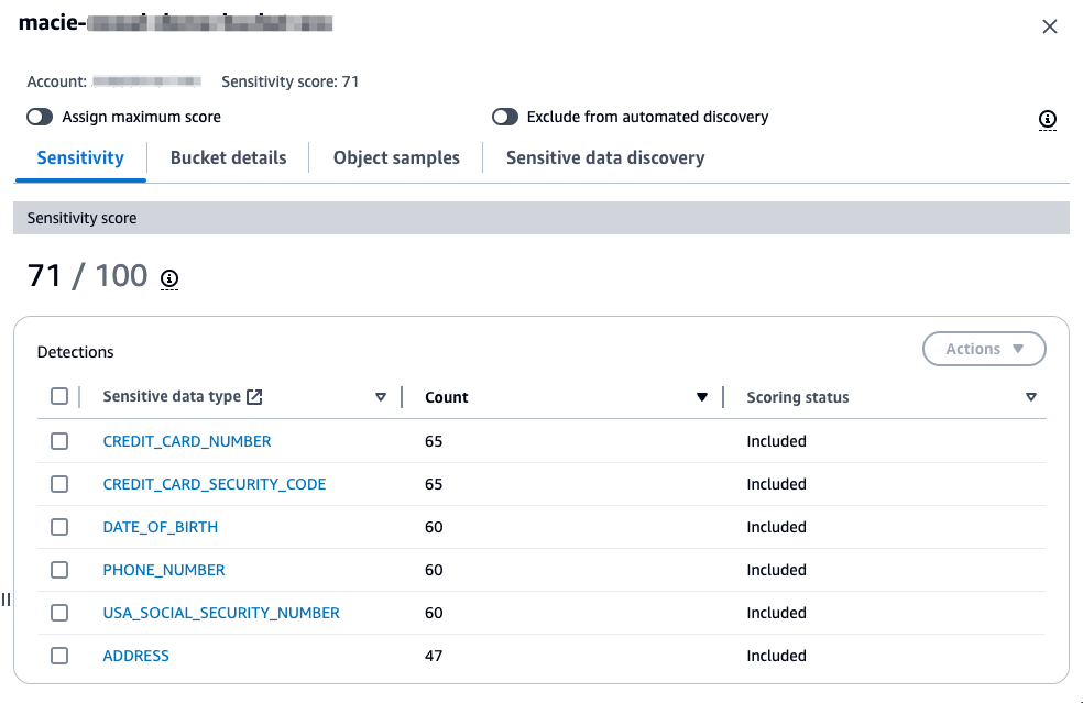
Amazon Macie is a data security service that discovers sensitive data using machine learning and pattern matching, provides visibility into data security risks, and enables automated protection against those risks. The following is a summary of the key features of Macie, many of which will be used in this POC. The core capabilities of Macie are focused on the security of your S3 buckets and helping to identify sensitive data including financial data, personal data, and credentials as well as sensitive data that’s unique to your organization, such as intellectual property.
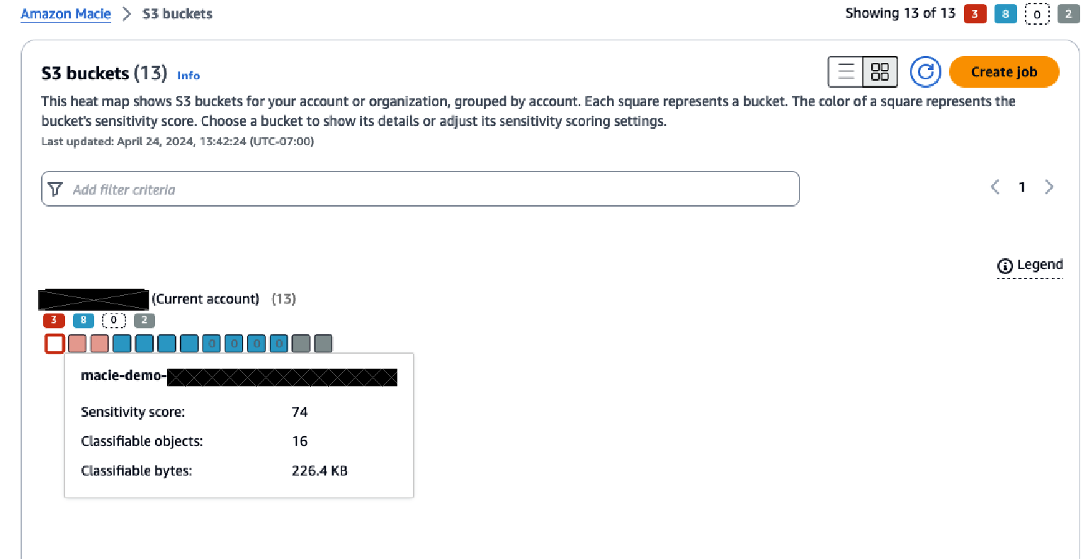
S3 bucket security
Customers use Amazon S3 for a variety of use cases and store various types of data in S3 buckets, including sensitive data. Continuously monitoring these buckets for the presence of sensitive data is a vital part of a data protection strategy. Macie gives you visibility into your S3 bucket inventory and the security and access controls associated with your buckets. This visibility includes if the bucket is publicly accessible, the encryption level of the bucket, and if the bucket is shared with other accounts. Whenever the security posture of one of your buckets is reduced, Macie generates a finding about the change, enabling you to respond. These findings are consumable through the AWS Management Console for Macie, through Macie APIs, as Amazon EventBridge messages, or through AWS Security Hub.
Sensitive data discovery jobs
Sensitive data discovery jobs provide a way to target a specific S3 bucket or group of buckets to do a deep analysis of the objects in those buckets and identify if sensitive data is present in the objects and if so, the type of data. These jobs can run on a daily, weekly, or monthly basis for new or changed data or once for on-demand analysis.
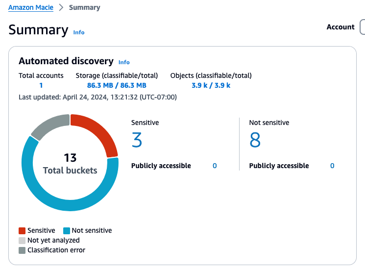
Automated data discovery
Macie offers an automated data discovery feature that can continually discover sensitive data within your S3 buckets. This feature is intended to help customers who have large amounts of S3 buckets and data better understand where sensitive data might be stored without having to scan all their data. By using automated data discovery, you can focus your resources on deeper investigations of the security of buckets identified to have sensitive data. Macie selects samples of the objects within S3 buckets and inspects them for the presence of sensitive data daily, providing insight into where sensitive data might reside in your overall Amazon S3 data estate.
POC overview
This POC is intended to help you gain an understanding of what Macie is capable of and how you can use it to achieve your data discovery goals. The POC in this post includes the following tasks in Macie:
Reviewing managed data identifiers
Defining custom data identifiers
Staging POC data
Running a sensitive data discovery job
Reviewing the output of the discovery job
Enabling and reviewing the output of automated data discovery
Note: The amount of time required for each task depends on your preparation and analysis for each stage. Note that, in the automated data discovery phase, it will take 24–48 hours for Macie to perform the first scan after the feature is enabled.
Enable Macie
Macie must be enabled before you can proceed with the POC. If you haven’t yet enabled Macie, see Enable Macie for instructions.
Note: When you enable Macie and the 30-day free trial for S3, monitoring S3 bucket security and privacy is automatically enabled. There’s also a 30-day free trial for automated data discovery, which is covered later in this post. There is no free trial for running targeted data discovery jobs. Review the Macie pricing page for details.
Review managed data identifiers
A successful POC of Macie includes understanding what data Macie can detect. Macie comes with over 150 managed data identifiers that are designed to identify sensitive data in your S3 objects. It’s important to first understand the available managed data identifiers and which ones align with the use cases you want to address. Examples of Macie managed data identifiers include credit card numbers, AWS secret access keys, and national identification numbers. Macie offers a default collection of recommend managed data identifiers to use for detecting general categories and types of sensitive data while optimizing data discovery results and reducing noise.
Keywords are an important component for Macie to be able to detect sensitive data. Many managed data identifiers require keywords to be in proximity of the data for Macie to be able to detect findings. Understanding the keywords that are used as part of sensitive data detection is important when it comes to building test data for a POC.
Prior to beginning your POC, review the list of managed data identifiers and determine which ones you feel will be necessary to use for your data discovery requirements. Additionally, identify which managed data identifiers, which are applicable to your POC, fall outside of the default list of identifiers.
Define custom data identifiers
Macie covers a wide number of use cases with its managed data identifiers, but some use cases need custom data identifiers for data types that aren’t included in the managed data identifiers. For example, customers might need to identify sensitive data that’s specific to their company, such as an employee ID or project number. Other customers might operate in industries that have data types unique to that industry, such as a known traveler number in the airline industry. If your requirements for identifying sensitive data include detecting sensitive data that isn’t part of the current list of managed data identifiers, then you can create custom data identifiers for those data types. For a POC, you might not want to create a custom data identifier for every additional detection. Instead, you can create a few to help confirm that you can use custom data identifiers for sensitive data detection and that Macie can support your data discovery goals. Building custom data identifiers has a thorough explanation of how to define a custom data identifier. Similar to managed data identifiers, custom data identifiers have keyword requirements. Defining detection criteria for custom data identifiers provides details for the types of data that require keywords.
Stage POC data
After reviewing the managed data identifiers provided by Macie and creating the custom data identifiers needed for your POC, it’s time to stage data sets that will help demonstrate the capabilities of these identifiers and better understand how Macie identifies sensitive data. We recommend that you stage data sets that contain sensitive data as well as data sets that do not to gain a full understanding of how Macie detects and reports on each of these situations. You can stage a variety of data sets to use for your POC using just a few GB of data to help keep your initial POC scans’ cost low. Staged data must be in file formats that Macie supports.
When preparing data to stage, keep in mind the keyword requirements for many of the Macie managed data identifiers. To determine which managed data identifiers have keyword requirements, see Managed data identifiers by type. When you’re staging your data, reference the keywords that are supported for the managed data identifiers you are using to help ensure that the data can be identified in your POC tests.
We recommend staging the data in one S3 bucket that’s dedicated to the POC and to use S3 server-side encryption on the bucket. If you want to use a customer managed AWS KMS key to encrypt the S3 data at rest, follow the instructions in Allowing Macie to use a customer managed AWS KMS key to give Macie access to decrypt the data in the bucket. You should also follow best practices for the S3 bucket related to not allowing public access and implementing least privilege access.
You can use one or more of the following approaches to identify and stage data for your POC:
Stage data files created by synthetic data generator tools with sensitive data included. There are many tools available for generating sensitive data. The following are two that you can use to generate test data.
Stage data files from public data repositories. There are various repositories staged with information that could be used for sensitive data detection. These repositories are often comprised of publicly available data sets or were created to help with testing machine learning models or sensitive data detection.
Stage data files of your own data with sensitive information. Because the goal is to use Macie to identify sensitive information in your S3 buckets, including examples of your own data that contains sensitive information can be helpful to test the capabilities of Macie.
Stage data files that don’t contain sensitive information. This can help you understand how Macie handles data that you believe doesn’t contain sensitive information. With the managed data identifiers that Macie offers, you should stage data files that you believe don’t contain information that aligns to the managed data identifiers. The staged data files could be log files, documents, or data sets that meet the criteria of this step.
Stage data that contains information that’s representative of data that you would want to detect using custom data identifiers.
Run a data classification job
Now that you’ve reviewed the managed data identifiers, defined custom data identifiers, and staged sample data, it’s time to run a sensitive data discovery job. When configuring the job scope, we recommend the following:
A specific S3 bucket where the POC data is staged.
The scope is set to be a one-time job.
Leave the sampling depth at 100 percent. Most customers leave this value at 100 percent, but some will lower it if they want a smaller random sample scan of their data. Most customers use automated data discovery to get sample scans instead of adjusting the sampling depth for individual jobs.
Select the recommended managed data identifiers. If your testing requires that Macie identify additional sensitive data types that are offered as managed data identifiers but aren’t part of the recommended list, choose the Custom option and select the managed data identifiers that you need. Make sure that the recommended managed data identifiers are part of the custom list that you construct.
Choose the custom data identifiers that you want to be used in the job.
After you configure your job, give it a name, review the final configuration, and then submit the job to run. A job that uses a data set of a few GB should complete within 30 minutes.
Review the findings from your job
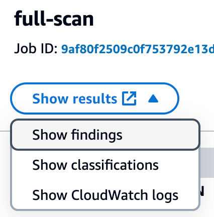
After the job completes, it’s time to review what Macie found in the data. Objects that Macie found with sensitive data will be presented as Findings in the Macie console. From the Jobs screen, choose the job you submitted. In the right-hand window, you will see the overview information for the job. From the overview window you can choose Show results menu and then select Show findings to view a list of the findings that were generated by the job.
Figure 1: Viewing Macie job findings
Each object where Macie found sensitive data will be listed as a single finding. If there were multiple types of sensitive data found in the object, each type of sensitive data and a count will be included in the details. Choose each of the findings that was produced and review the details to confirm what sensitive data was identified and if the sensitive data was discovered as you expected. Additionally, confirm that you don’t have findings for objects that you staged that were not supposed to have sensitive data so that you can confirm how Macie handles these types of objects. If you created custom data identifiers, review findings for the objects that included the custom data that you detect to confirm that the data was detected.
Enable automated discovery
Now that you understand how to use Macie to discover sensitive data, the next step in the POC is to enable automated discovery and use Macie to discover sensitive data across a larger collection of your existing S3 data.
You will be enabling automated discovery in Macie as a 30-day free trial. For the free trial, the scope of total data storage to be evaluated will be 150 GB. Use the following steps to guide your setup of the automated discovery feature:
After your delegated administrator account is configured, enable automated discovery. As part of enabling automated discovery, pay extra attention to the following items:
Set managed data identifiers. Ideally, choose the recommended data identifiers to help reduce noise. If there are specific managed data identifiers that you really want to see, then choose Custom to choose the ones you want.
Include custom data identifiers that you want to be used to evaluate your sensitive data.
Exclude buckets that you don’t want included in the scope for identifying sensitive data.
Include or exclude specific accounts that should be part of the POC. Step 5 of Enable automated discovery covers how to enable it for specific accounts.
You will see the first set of results 24 to 48 hours after you enable automated discovery. After that, you will see updates to the automated discovery results every 24 hours.
After automated discovery starts producing results, you will start seeing data in the Automated Discovery section of the Macie summary page in the console. The summary includes metrics for the total number of buckets eligible for discovery, counts for the number of buckets where sensitive data was or was not found, and how many of these buckets are public.
Figure 2: Example automated discovery summary metrics
Choosing a link for one of the counts will take you to the S3 buckets view with the appropriate filters applied.
After reviewing the summary screen, choose S3 buckets from the navigation pane to see a heatmap that shows each account and the buckets within each account.
Figure 3: S3 bucket heatmap view in Macie
The heatmap provides point-in-time insights into the data that Macie has scanned, and in which buckets sensitive data has been identified or no sensitive data has been found.
Over time, this heatmap might change as automated data discovery continues sampling the data in each bucket. The heatmap view provides information on each organizational member account and insight about sensitive data within each bucket in the account.
The console displays the results as a set of colored squares for each account. Each square represents a bucket in that account and the color of the square indicates whether sensitive data was discovered in that bucket. Red indicates that some type of sensitive data has been found in the bucket, while blue indicates no sensitive data has been identified. If a bucket is blue, that means only that automated data discovery hasn’t identified sensitive data up to the point in time of the last scan, not that there is no sensitive data in the bucket.
Hover over each bucket to see a summary of the sensitivity score of the bucket along with statistics about the data in the bucket. Choosing a bucket in the heatmap will open a window that provides more information about the bucket. This information includes the sensitivity score of the bucket, a summary of the types of sensitive data found in the bucket, which objects within the bucket have been sampled, statistics related to the data that has been scanned and data that is still to be scanned, and other information about the bucket.
Figure 4: S3 bucket sensitivity information in Macie
As part of your POC, it’s recommended that you investigate buckets that are reported to contain sensitive data. For your investigation, validate if the data identified is sensitive based on your organization’s data classification policy. Each Macie finding contains not only the details on the types of sensitive data identified, but also the location within the file where the sensitive data is located so that you can confirm the identified data is sensitive. The following is an example of a Macie finding in an Excel file where bank account numbers were found. This example shows the row and column where the sensitive data was found.
Investigating sensitive data with findings has detailed guidance around locating sensitive data from Macie findings, retrieving the sensitive data, and the schema for sensitive data locations. If the findings are true positives, make sure that the bucket has the right level of security configurations and permissions based on the data stored in the bucket.
In addition to reviewing the bucket level statistics that are generated by automated discovery, you can view the individual findings that were generated for each S3 object that was identified as having sensitive data. You can view the findings through the Findings tab in Macie or by choosing the sensitive data type when looking at the summary detections for a bucket.
Next steps
With the preceding POC, you should now have a more complete understanding of how Macie identifies sensitive data and how you can use the information that Macie provides about that data identified. As you complete your POC, there are a few next steps that other customers have taken after completing their POC with Macie.
Operationalize Macie output
In the POC steps, we outlined how to view the findings and the insights that the automated discovery provides. Before you proceed with Macie, you should have a plan for how you will operationalize the Macie output. This will help ensure that the remediation steps for identified sensitive data are directed to the correct parties.
Depending on what operational tools you have in place, the steps that you take to operationalize the output of Macie will vary. Many customers implement operational processes that cover the following areas:
The privacy or security team that’s responsible for Macie does an initial triage on the findings to confirm if there are true positives.
The privacy or security team defines their operational processes related to the summary dashboard and bucket sensitivity information that’s provided by automated discovery.
The team that owns the bucket where the sensitive data is located is provided the information needed to investigate the identified data and provide a response. Responses will vary but could include removal of the data, correcting the application that is writing the data, or applying additional security to the bucket.
A key part of operationalizing Macie output is also how you are getting and reviewing the signals related to Macie findings. As outlined in this post, you can view and investigate findings in the Macie console. At a steady state, customers find it beneficial to consume Macie findings using Amazon EventBridge, through Macie APIs, or through the integration of Macie with AWS Security Hub. These options can be used to incorporate the findings that are reported by Macie into the operational workflows and tools that work best for your organization and allow you to consume and address findings at scale. Monitoring and processing findings provides more insight into these integration approaches.
Store and retain sensitive data discovery results
As you move forward with Macie, it’s important to enable logging for each of the S3 objects that Macie has scanned. Macie creates an analysis record for each S3 object that’s in scope for a data discovery job or an automated discovery scan. These records are an audit of every object that Macie attempted to scan, including objects that didn’t contain sensitive data. Data discovery results are written to an S3 bucket that you own and where you control the data retention. These data discovery results can assist with analysis of records over time or to get a broader sense of what data Macie has scanned and which objects had sensitive data and which did not.
The data discovery scan results are stored as JSON Lines files. You can use multiple approaches to analyze and query these log files. The Amazon Macie Results Analytics GitHub repository provides instructions on how to configure Amazon Athena with tables that allow you to query the results of Macie discovery scan files.
Define the scope for Macie use
After a POC with Macie, you can set the scope of how you will use Macie in production by deciding which buckets don’t need to be evaluated and so can be excluded, such as buckets used for AWS logs and buckets deemed not in scope for sensitive data identification.
You can also refine the managed data identifiers that are required for detecting sensitive data. Based on what they learned from the POC. You can create custom data identifiers to help meet your data detection needs if necessary.
As you identify the sensitive data discovery jobs to run as part of your production use of Macie, keep in mind that these jobs are immutable. To edit an existing scheduled job, you must create a copy of the job with the updated configuration and cancel the original job for changes to take effect. Depending on the updated criteria for your job, you must do one of the following to help avoid re-scanning objects that were covered by the previous job:
Clear include existing objects when setting the scope. This will cause the new job to schedule only objects that were created between when it was first created and when it was run for the first time.
When setting the job scope, set the object attributes so that the object last modified date is the date of the last time the previous job ran. This helps ensure that when the new scheduled job runs, it evaluates only objects that weren’t covered by the previous job.
Clean up
To avoid incurring additional charges, disable Macie while you evaluate the value of the additional data protection provided. If S3 buckets were created for this POC, those should also be deleted.
Call to action
After the POC is complete, evaluate the results to determine how much using Macie can strengthen your organization’s data protection program. Based on that evaluation, you can identify how and where to use Macie for maximum effectiveness. Also consider how the information provided can be factored into operational workflows to get additional value from Macie.
Conclusion
This post outlined how you can use a POC to better understand how Amazon Macie can help meet your data discovery and classification needs. A well thought-out and implemented POC can provide valuable early insights and help you develop a more thorough understanding of what your data discovery and classification strategy should be. Planning your POC using the guidance in this post can help you determine more quickly if Macie is a fit for your company.
If you have feedback about this post, submit comments in the Comments section below. If you have questions about this post, contact AWS Support.
Today, NICE DCV has a new name. So long NICE DCV, welcome Amazon DCV. Today, with the 2024.0 release, along with enhancements and bug fixes, NICE DCV is rebranded to Amazon DCV.
The new name is now also used to consistently refer to the DCV protocol powering AWS managed services such as Amazon AppStream 2.0 and Amazon WorkSpaces.
What is Amazon DCV Amazon DCV is a high-performance remote display protocol. It lets you securely deliver remote desktops and application streaming from any cloud or data center to any device, over varying network conditions. By using Amazon DCV with Amazon Elastic Compute Cloud (Amazon EC2), you can run graphics-intensive applications remotely on EC2 instances. You can then stream the results to more modest client machines, which eliminates the need for expensive dedicated workstations.
Amazon DCV supports both Windows and major flavors of Linux operating systems on the server side, providing you flexibility to fit your organization’s needs. The client-side that receives the desktops and application streamings could be the native DCV client for Windows, Linux, or macOS or web browsers. The DCV remote server and client transfer only encrypted pixels, not data, so no confidential data is downloaded from the DCV server. When you choose to use Amazon DCV on Amazon Web Services (AWS) with EC2 instances, you can take advantage of the AWS 108 Availability Zones across the 33 geographic Regions and 31 local zones, allowing your remote streaming services to scale globally.
Since Amazon acquired NICE 8 years ago, we’ve witnessed a diverse range of customers adopting DCV. From general-purpose users visualizing business applications to industry-specific professionals, DCV has proven to be versatile. For instance, artists have employed DCV to access powerful cloud workstations for their digital content creation and rendering tasks. In the healthcare sector, medical imaging professionals have used DCV for remote visualization and analysis of patient data. Geoscientists have used DCV to analyze reservoir simulation results, while engineers in manufacturing have used it to visualize computational fluid dynamics experiments. The education and IT support industries have benefited from collaborative sessions in DCV, in which multiple users can share a single desktop.
Notable customers include Quantic Dream, an award-winning game development studio that has harnessed DCV to create high-resolution, low-latency streaming services for their artists and developers. Tally Solutions, an enterprise resource planning (ERP) services provider, has employed DCV to securely stream its ERP software to thousands of customers. Volkswagen has used DCV to provide remote access to computer-aided engineering (CAE) applications for over 1,000 automotive engineers. Amazon Kuiper, an initiative to bring broadband connectivity to underserved communities, has used DCV for designing complex chips.
Within AWS, DCV has been adopted by several services to provide managed solutions to customers. For example, AppStream 2.0 uses DCV to offer secure, reliable, and scalable application streaming. Additionally, since 2020, Amazon WorkSpaces Streaming Protocol (WSP), which is built on DCV and optimized for high performance, is available for Amazon WorkSpaces customers. Today, we’re also phasing out the WSP name and replacing it with DCV. Going forward, you will have DCV as a primary protocol choice in Amazon WorkSpaces.
What’s new with version 2024.0 Amazon DCV 2024.0 introduces several fixes and enhancements for improved performance, security, and ease of use. The 2024.0 release now supports the latest Ubuntu 24.04 LTS, bringing the latest security updates and extended long-term support to simplify system maintenance. The DCV client on Ubuntu 24.04 has built in support for Wayland, offering better graphical rendering efficiency and enhanced application isolation. Additionally, DCV 2024.0 now enables the QUIC UDP protocol by default, allowing clients to benefit from an optimized streaming experience. The release also introduces the capability to blank the Linux host screen when a remote user is connected, preventing local access and interaction with the remote session.
How to get started The easiest way to test DCV is to spin up a WorkSpaces instance from the WorkSpaces console, selecting one of the DCV-powered bundles, or creating an AppStream session. For this demo however, I want to show you how to install DCV server on an EC2 instance.
The Windows installation is straightforward: start the msi file, select Next at each step and voilà. It was installed in less time than it took me to write this sentence.
The installation on Linux deserves a bit more care. Amazon Machine Images (AMI) for EC2 servers don’t include any desktop or graphical components. As a prerequisite, I had to install the X Window System and a window manager, and configure X to let users connect and start a graphical user interface session on the server. Fortunately, all these steps are well documented. Here is a summary of the commands I used.
After the reboot, I installed the DCV server package
# Install the server
$ sudo apt install ./nice-dcv-server_2024.0.17794-1_amd64.ubuntu2404.deb
$ sudo apt install ./nice-xdcv_2024.0.625-1_amd64.ubuntu2404.deb

# (optional) install the DCV web viewer to allow clients to connect from a web browser
$ sudo apt install ./nice-dcv-web-viewer_2024.0.17794-1_amd64.ubuntu2404.deb
$ sudo dcv list-sessions
There are no sessions available.

$ sudo dcv create-session console --type virtual --owner seb

$ sudo dcv list-sessions
Session: 'console' (owner:seb type:virtual)
Once my server configuration was ready, I started the DCV client on my laptop. I only had to enter the IP address of the server and the username and password of the user to initiate a session.
On my laptop, I opened a new DCV client window and connected to the other EC2 server. After a few seconds, I was able to remotely work with the Windows and the Ubuntu machine running in the cloud.
Pricing and availability Amazon DCV is free of charges when used on AWS. You only pay for the usage of AWS resources or services, such as EC2 instances, Amazon Workspace desktops, or Amazon App Stream 2.0. If you plan to use DCV with on-premises servers, check the list of license resellers on our website.
Version 7.1 of
the FFmpeg audio/video toolkit has been released. Important changes in
this release include the VVC decoder reaching stable status, and
inclusion of support for MV-HEVC decoding (which is generated by
recent phones and VR headsets), as well as support for Vulkan encoding
with H264 and HEVC. See the announcement and changelog
for full details.
The collective thoughts of the interwebz
Manage Consent
To provide the best experiences, we use technologies like cookies to store and/or access device information. Consenting to these technologies will allow us to process data such as browsing behavior or unique IDs on this site. Not consenting or withdrawing consent, may adversely affect certain features and functions.
Functional
Always active
The technical storage or access is strictly necessary for the legitimate purpose of enabling the use of a specific service explicitly requested by the subscriber or user, or for the sole purpose of carrying out the transmission of a communication over an electronic communications network.
Preferences
The technical storage or access is necessary for the legitimate purpose of storing preferences that are not requested by the subscriber or user.
Statistics
The technical storage or access that is used exclusively for statistical purposes.The technical storage or access that is used exclusively for anonymous statistical purposes. Without a subpoena, voluntary compliance on the part of your Internet Service Provider, or additional records from a third party, information stored or retrieved for this purpose alone cannot usually be used to identify you.
Marketing
The technical storage or access is required to create user profiles to send advertising, or to track the user on a website or across several websites for similar marketing purposes.
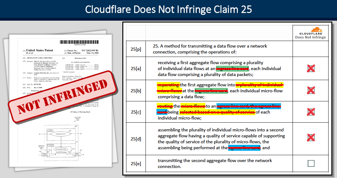
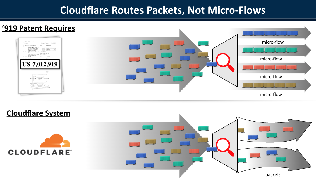
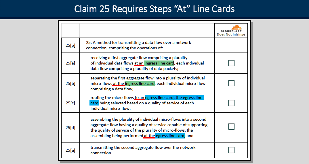

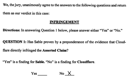
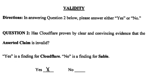


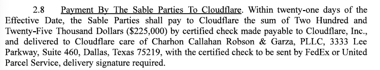
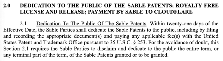
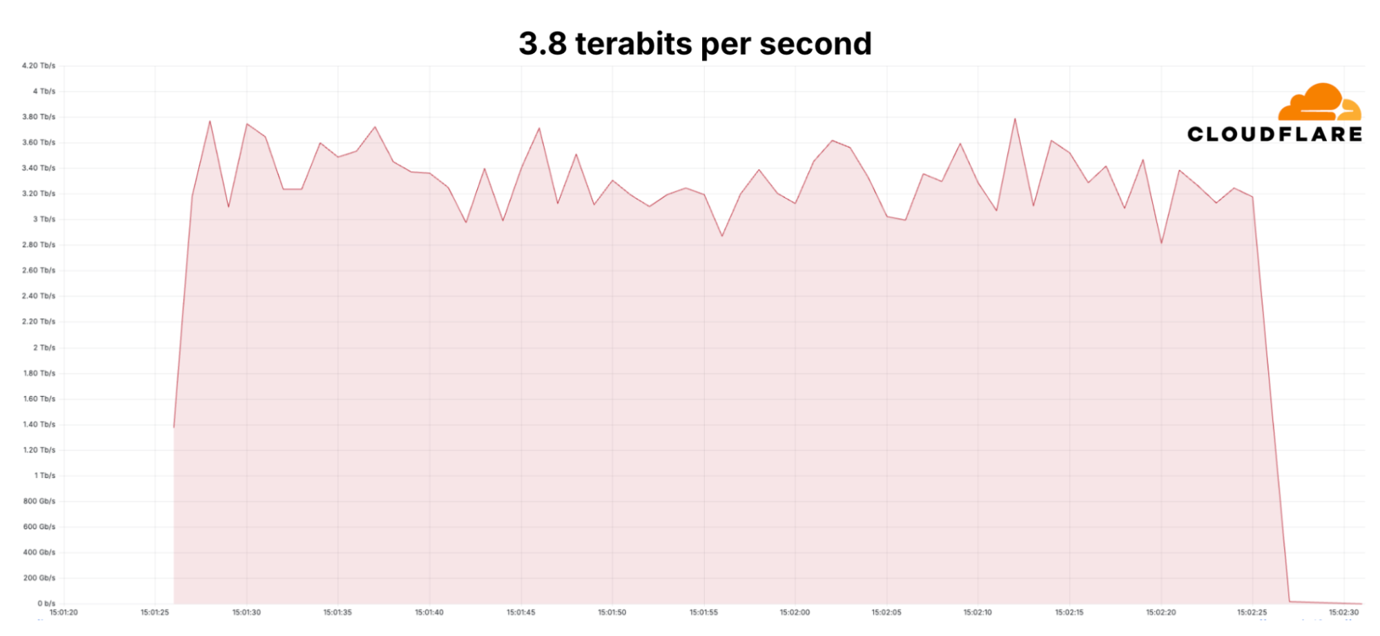
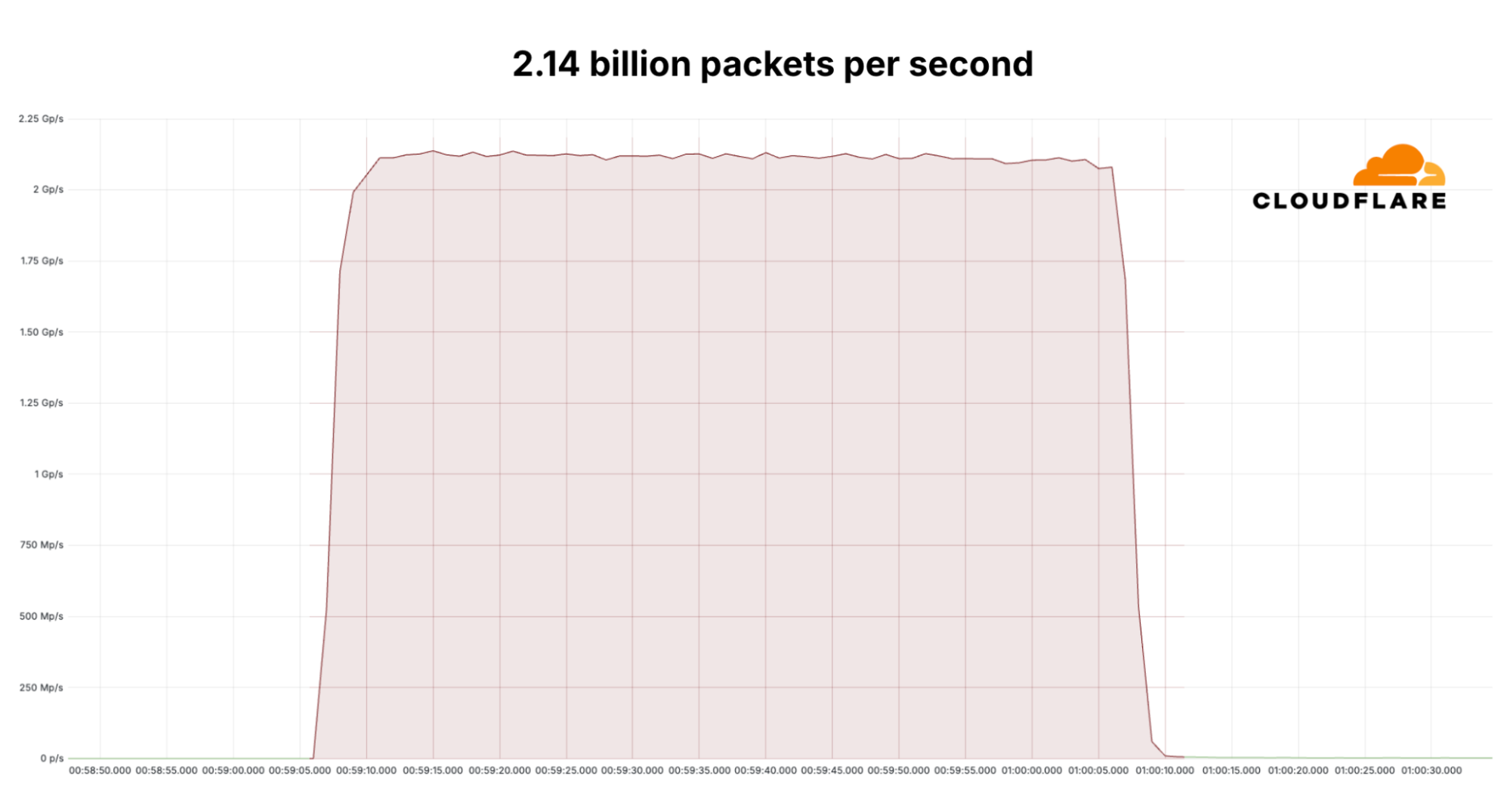
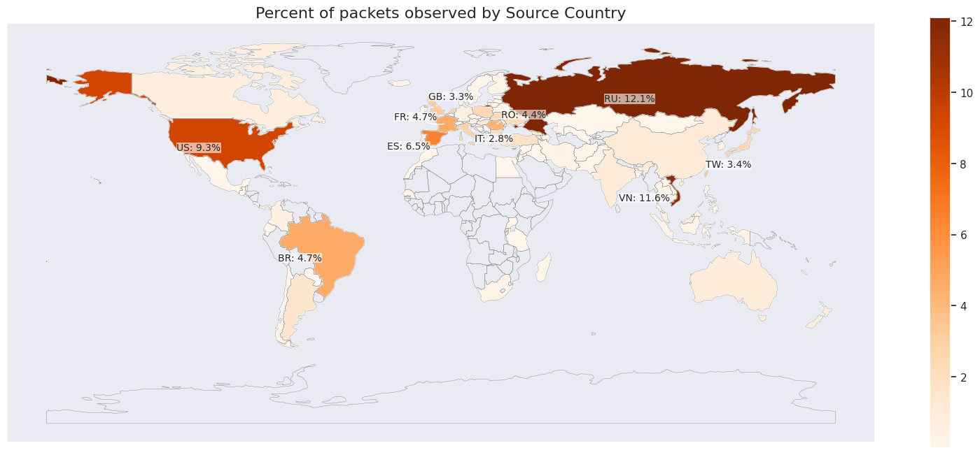
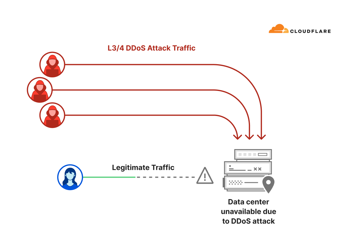


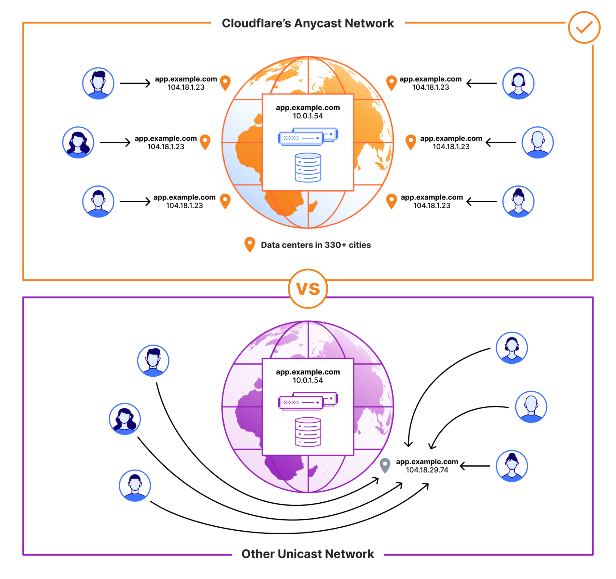
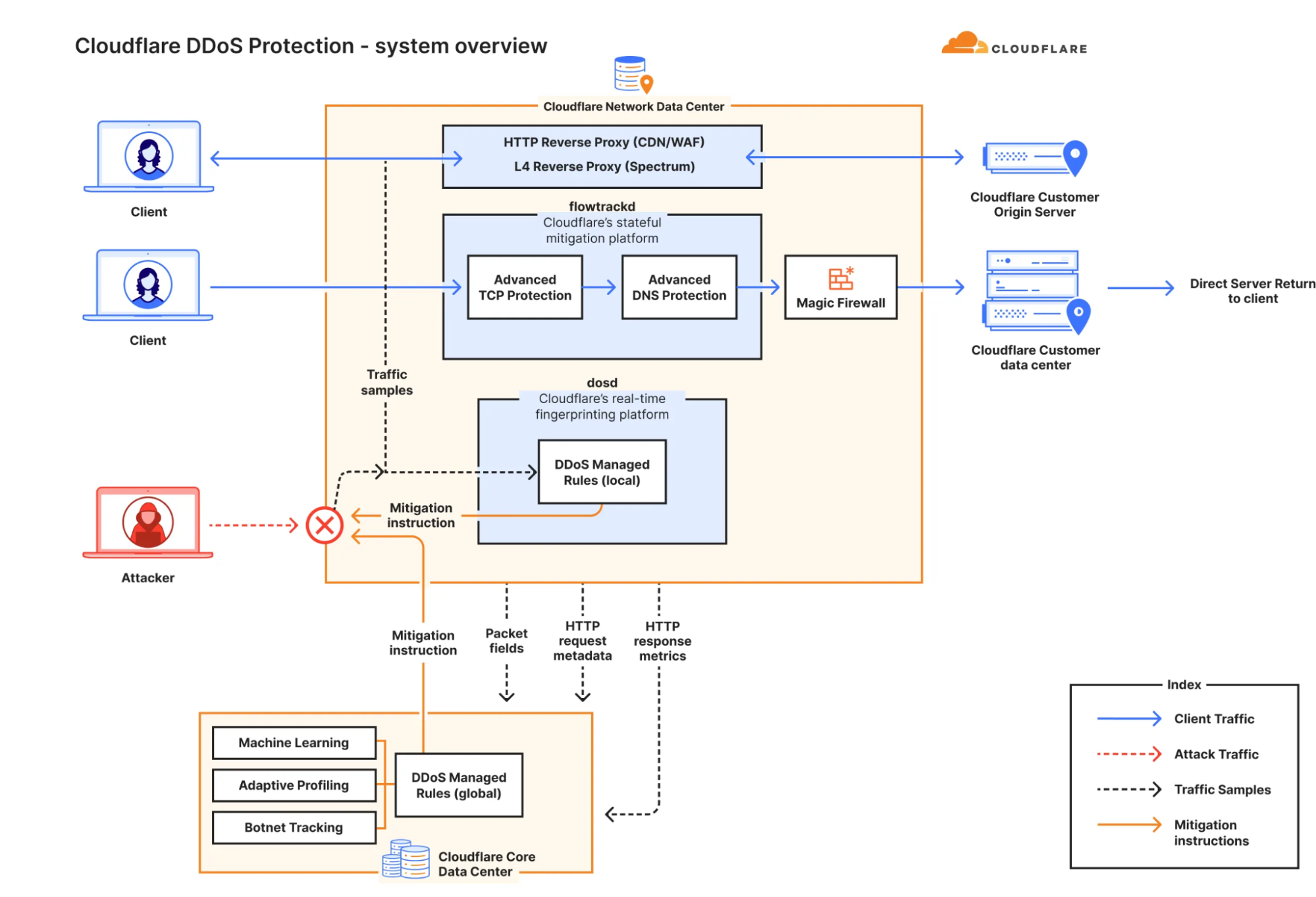


 Kalaiselvi Kamaraj is a Sr. Software Development Engineer with Amazon. She has worked on several projects within Redshift Query processing team and currently focusing on performance related projects for Redshift Data Lake.
 Mark Lyons is a Principal Product Manager on the Amazon Redshift team. He works on the intersection of data lakes and data warehouses. Prior to joining AWS, Mark held product leadership roles with Dremio and Vertica. He is passionate about data analytics and empowering customers to change the world with their data.
 Asser Moustafa is a Principal Worldwide Specialist Solutions Architect at AWS, based in Dallas, Texas, USA. He partners with customers worldwide, advising them on all aspects of their data architectures, migrations, and strategic data visions to help organizations adopt cloud-based solutions, maximize the value of their data assets, modernize legacy infrastructures, and implement cutting-edge capabilities like machine learning and advanced analytics. Prior to joining AWS, Asser held various data and analytics leadership roles, completing an MBA from New York University and an MS in Computer Science from Columbia University in New York. He is passionate about empowering organizations to become truly data-driven and unlock the transformative potential of their data.