The “limited” C API for CPython extensions has been around for well over a
decade at this point, but it has not seen much uptake. It is meant to give
extensions an API that will allow binaries built with it to be used for
multiple versions of CPython, because those binaries will only access the stable
ABI that will not change when CPython does. Victor Stinner has been
working on better
definition for the
API; as part of that work, he suggested that some of the C extensions in the
standard
library start using it in an effort for CPython to “eat its
own dog food“. The resulting discussion showed that there is still a fair
amount of confusion about this API—and the thrust of Stinner’s overall plan.
Amazon CodeCatalyst is a unified software development service for building and delivering applications on AWS. With CodeCatalyst, you can implement your team’s preferred branching strategy. Whether you follow popular models like GitFlow or have your own approach, CodeCatalyst Workflows allow you to design your development process and deploy to multiple environments.
Introduction
In a previous post in this series, Using Workflows to Build, Test, and Deploy with Amazon CodeCatalyst, we discussed creating a continuous integration and continuous delivery (CI/CD) pipeline in CodeCatalyst and how you can continually deliver high-quality updates through the use of one workflow. I will build on these concepts by focusing on how you collaborate across your codebase by using multiple CodeCatalyst Workflows to model your team’s branching strategy.
Having a standardized process for managing changes to the codebase allows developers to collaborate predictably and focus on delivering software. Some popular branching models include GitFlow, GitHub flow, and trunk-based development.
GitFlow is designed to manage large projects with parallel development and releases, featuring multiple long-running branches.
GitHub flow is a lightweight, branch-based workflow that involves creating feature branches and merging changes into the main branch.
Trunk-based development is focused on keeping the main branch always stable and deployable. All changes are made directly to the main branch, and issues are identified and fixed using automated testing and deployment tools.
In this post, I am going to demonstrate how to implement GitFlow with CodeCatalyst. GitFlow uses two permanent branches, main and develop, with supporting branches. The prefix names of the supporting branches give the function they serve — feature, release, and hotfix. I will apply this strategy by separating these branches into production and integration, both with their own workflow and environment. The main branch will deploy to production and the develop branch plus the supporting branches will deploy to integration.
Figure 1. Implementing GitFlow with CodeCatalyst.
Upon completing the walkthrough, you will have the ability to utilize these techniques to implement any of the popular models or even your own.
Prerequisites
If you would like to follow along with the walkthrough, you will need to:
Have an AWS account associated with your space and have the IAM role in that account. For more information about the role and role policy, see Creating a CodeCatalyst service role.
Walkthrough
For this walkthrough, I am going use the Static Website blueprint with the default configuration. A CodeCatalyst blueprint creates new project with everything you need to get started. To try this out yourself, launch the blueprint by following the steps outlined in the Creating a project in Amazon CodeCatalyst.
Once the new project is launched, I navigate to CI/CD > Environments. I see one environment called production. This environment was setup when the project was created by the blueprint. I will now add my integration environment. To do this, I click the Create environment above the list of environments.
Figure 2. Initial environment list with only production.
A CodeCatalyst environment is where code is deployed and are configured to be associated with your AWS account using AWS account connections. Multiple CodeCatalyst environments can be associated with a single AWS account, allowing you to have environments in CodeCatalyst for development, test, and staging associated with one AWS account.
In the next screen, I enter the environment name as integration, select Non-production for the environment type, provide a brief description of the environment, and select the connection of the AWS account I want to deploy to. To learn more about connecting AWS accounts review Working with AWS accounts in Amazon CodeCatalyst. I will make note of my connection Name and Role, as I will need it later in my workflow. After I have entered all the details for the integration environment, I click Create environment on the bottom of the form. When I navigate back to CI/CD > Environments I now see both environments listed.
Figure 3. Environment list with integration and production.
Now that I have my production and integration environment, I want to setup my workflows to deploy my branches into each separate environment. Next, I navigate to CI/CD > Workflows. Just like with the environments, there is already a workflow setup by the blueprint created called OnPushBuildTestAndDeploy. In order to review the workflow, I select Edit under the Actions menu.
By reviewing the workflow YAML, I see the OnPushBuildTestAndDeploy workflow is triggered by the main branch and deploys to production. Below I have highlighted the parts of the YAML that define each of these. The Triggers in the definition determine when a workflow run should start and Environment where code is deployed to.
Since this confirms the production workflow is already done, I will copy this YAML and use it to create my integration workflow. After copying the entire OnPushBuildTestAndDeploy YAML to my clipboard (not just the highlights above), I navigate back to CI/CD > Workflows and click Create Workflow. Then in the Create workflow dialog window click Create.
Figure 5. Create workflow dialog window.
Inside the workflow YAML editor, I replace all the existing content by pasting the OnPushBuildTestAndDeploy YAML from my clipboard. The first thing I edit in the YAML is the name of the workflow. I do this by finding the property called Name and replacing OnPushBuildTestAndDeploy to OnIntegrationPushBuildTestAndDeploy.
Next, I want to change the triggers to the develop branch and match the supporting branches by their prefixes. Triggers allow you to specify multiple branches and you can use regex to define your branch names to match multiple branches. To explore triggers further read Working with triggers.
After my triggers are updated, I need to update the Environment property with my integration environment. I replace both the Name and the Connections properties with the correct values for my integration environment. I use the Name and Role from the integration environment connection I made note of earlier. For additional details about environments in workflows review Working with environments.
Before finishing the integration workflow, I have highlighted the use of ${WorkflowSource.BranchName} in the Deploy action. The workflow uses the BranchName variable to prevent different branch deployments from overwriting one another. This is important to verify as all integration branches use the same environment. The WorkflowSource action outputs both CommitId and BranchName to workflow variables automatically. To learn more about variables in workflows review Working with variables.
I have included the complete sample OnIntegrationPushBuildTestAndDeploy workflow below. It is the developer’s responsibility to delete resources their branches create even after merging and deleting branches as there is no automated cleanup.
Figure 6. Entire sample integration workflow.
After I have validated the syntax of my workflow by clicking Validate, I then click Commit. Confirm this action by clicking Commit in the Commit workflow modal window.
Figure 7. Commit workflow dialog window.
Immediately after committing the workflow, I can see the new OnIntegrationPushBuildTestAndDeploy workflow in my list of workflows. I see that the workflow shows the “Workflow is inactive”. This is expected as I am looking at the main branch and the trigger is not invoked from main.
Now that I have finished the implementation details of GitFlow, I am now going to create the permanent develop branch and a feature branch to test my integration workflow. To add a new branch, I go to Code > Source repositories > static-website-content, select Create branch under the More menu.
Figure 8. Source repository Actions menu.
Enter develop as my branch name, create the branch from main, and then click Create.
Figure 9. Create the develop branch from main.
I now add a feature branch by navigating back to the create branch screen. This time, I enter feature/gitflow-demo as my branch name, create the branch from develop, and then click Create.
Figure 10. Create a feature branch from develop.
To confirm that I have successfully implemented GitFlow, I need to verify that the feature branch workflow is running. I return to CI/CD > Workflows, select feature/gitflow-demo from the branch dropdown, and see the integration workflow is running.
To complete my testing of my implementation of GitFlow, I wait for the workflow to succeed. Then I view the newly deployed branch by navigating to the workflow and clicking on the View app link located on the last workflow action.
Lastly, now that GitFlow is implemented and tested, I will step through getting the feature branch to production. After I make my code changes to the feature branch, I create a pull request to merge feature/gitflow-demo into develop. Note that pull requests were covered in the prior post in this series. When merging the pull request select Delete the source branch after merging this pull request, as the feature branch is not a permanent branch.
Figure 12. Deleting the feature branch when merging.
Now that my changes are in the develop branch, I create a release branch. I navigate back to the create branch screen. This time I enter release/v1 as my branch name, create the branch from develop, and then click Create.
Figure 13. Create the release branch from main.
I am ready to release to production, so I create a pull request to merge release/v1 into main. The release branch is not a permanent branch, so it can also be deleted on merge. When the pull request is merged to main, the OnPushBuildTestAndDeploy workflow runs. After the workflow finishes running, I can verify my changes are in production.
Cleanup
If you have been following along with this workflow, you should delete the resources you deployed so you do not continue to incur charges. First, delete the two stacks that deployed using the AWS CloudFormation console in the AWS account(s) you associated when you launched the blueprint and configured the new environment. These stacks will have names like static-web-XXXXX. Second, delete the project from CodeCatalyst by navigating to Project settings and choosing Delete project.
Conclusion
In this post, you learned how to use triggers and environments in multiple workflows to implement GitFlow with Amazon CodeCatalyst. By consuming variables inside workflows, I was able to further customize my deployment design. Using these concepts, you can now implement your team’s branching strategy with CodeCatalyst. Learn more about Amazon CodeCatalyst and get started today!
This week, Rapid7 was named a Strong Performer in The Forrester Wave™: Vulnerability Risk Management, Q3 2023. The report, which included 11 vulnerability risk management vendors, represented Rapid7’s inclusion in the Wave report for vulnerability management. We are proud to be recognized for our consolidated platform approach, speedy response to actively exploited emergency vulnerabilities, and a deep commitment to the cybersecurity community through open-source tools and community research.
As organizations move to the cloud, security teams need to adapt their vulnerability management programs to secure their ever-increasing attack surface, including both on-premise assets and more ephemeral cloud resources. While the market has many tools that security teams can use to meet specific use cases—either a component of vulnerability management process or specific technology like Cloud or OT or applications—working with multiple tools/solutions can add to challenges of security operations.
As a result, security teams are continually leaning toward vendors who can consolidate their security needs. Gartner recently stated that “Seventy-five percent of organizations are pursuing a security vendor consolidation—in 2020, this figure was only 29%. More organizations consolidate to improve risk posture than to save on budget.*” Rapid7 will continue to build a consolidated, practitioner-first platform that helps security teams meet their vulnerability management and compliance needs for a hybrid environment with a single solution.
Building A Comprehensive Risk Management Solution
Our Cloud Risk Complete solution unifies on-prem risk management, cloud security, and application security testing with a practitioner-first approach. It offers security teams:
Visibility in their attack surface – Unlock a comprehensive view of risk across applications, cloud environments, and on-prem infrastructure. Forrester gave Rapid7 the perfect score for comprehensive coverage of assets across hybrid environments and provides valuable information regarding assets for several types of remediation teams across a typical enterprise. Our asset coverage includes cloud service providers like AWS, Azure, GCP, Oracle & Alibaba; Applications; Infrastructure – Networking devices; Data; Operating systems and software; OT/IoT coverage; Web Applications and APIs
Unlimited risk assessment – Accelerate risk assessment with purpose-built solutions that scan and assess each environment. Our agentless approach in cloud environments allows customers to auto detect new resources and configuration changes within seconds. Project SONAR provides external attack surface visibility. In addition to native scanning capabilities, we continually add to our partner ecosystem and integrations, particularly ingesting 3rd-party assets, including IoT/OT, to help customers maintain complete asset inventory.
Enforce compliance and accelerate remediation – A successful VM program looks to remediate risk, efficiently with minimal manual intervention. Rapid7 provides several ways to automate remediation-related tasks – for instance, killing non-gold images and searching for vulnerable applications and containing them – for which Forrester provided us with perfect scores.The built-in automated workflows and third-party integrations (both customizable) helps security teams to drive collaboration and remediate risk faster.
Drive operational efficiency and results – with a single vendor that has industry leading solutions across cloud environments, applications and on-prem infrastructure.
As part of helping Security teams reduce risk posed by actively exploited vulnerabilities, our Emergent Threat Response (ETR) program flags multiple CVEs as part of an ongoing process to deliver fast, expert analysis alongside first-rate security content for the highest-priority security threats. You can learn more about the recent threats we have disclosed or responded to here.
As we continue to double down on our strategy of providing a consolidated, comprehensive risk management platform, we’ve made a number of recent investments and product releases, including:
Enterprise Risk View – provides the visibility and context needed to track total risk across the entire attack surface (cloud and on-prem) and understand organizational risk posture.
Attack Path Analysis – visualize risk across cloud environments in real-time, mapping relationships between compromised resources and the rest of the environment.
Active Risk – a unified vulnerability risk scoring and prioritization strategy across hybrid environments
“Rapid7 has been a reliable and effective tool allowing us to reduce our vulnerabilities by over 95% and effectively maintain a well patched, well configured environment”. – Director of Cybersecurity at Kutak Rock LLP.
Thank you to our customers and partners for always supporting and guiding us! We’re excited to keep investing in a platform that helps security teams prevent and manage risk from the endpoint to the cloud and simplify security operations.
*Source: Gartner, Inc: Top Trends in Cybersecurity — Survey Analysis: Cybersecurity Platform Consolidation, Dionisio Zumerle, John Watt, February 22, 2023
Almost three years ago, we launched Cloudflare Waiting Room to protect our customers’ sites from overwhelming spikes in legitimate traffic that could bring down their sites. Waiting Room gives customers control over user experience even in times of high traffic by placing excess traffic in a customizable, on-brand waiting room, dynamically admitting users as spots become available on their sites. Since the launch of Waiting Room, we’ve continued to expand its functionality based on customer feedback with features like mobile app support, analytics, Waiting Room bypass rules, and more.
We love announcing new features and solving problems for our customers by expanding the capabilities of Waiting Room. But, today, we want to give you a behind the scenes look at how we have evolved the core mechanism of our product–namely, exactly how it kicks in to queue traffic in response to spikes.
How was the Waiting Room built, and what are the challenges?
The diagram below shows a quick overview of where the Waiting room sits when a customer enables it for their website.
Waiting Room is built on Workers that runs across a global network of Cloudflare data centers. The requests to a customer’s website can go to many different Cloudflare data centers. To optimize for minimal latency and enhanced performance, these requests are routed to the data center with the most geographical proximity. When a new user makes a request to the host/path covered by the Waiting room, the waiting room worker decides whether to send the user to the origin or the waiting room. This decision is made by making use of the waiting room state which gives an idea of how many users are on the origin.
The waiting room state changes continuously based on the traffic around the world. This information can be stored in a central location or changes can get propagated around the world eventually. Storing this information in a central location can add significant latency to each request as the central location can be really far from where the request is originating from. So every data center works with its own waiting room state which is a snapshot of the traffic pattern for the website around the world available at that point in time. Before letting a user into the website, we do not want to wait for information from everywhere else in the world as that adds significant latency to the request. This is the reason why we chose not to have a central location but have a pipeline where changes in traffic get propagated eventually around the world.
This pipeline which aggregates the waiting room state in the background is built on Cloudflare Durable Objects. In 2021, we wrote a blog talking about how the aggregation pipeline works and the different design decisions we took there if you are interested. This pipeline ensures that every data center gets updated information about changes in traffic within a few seconds.
The Waiting room has to make a decision whether to send users to the website or queue them based on the state that it currently sees. This has to be done while making sure we queue at the right time so that the customer's website does not get overloaded. We also have to make sure we do not queue too early as we might be queueing for a falsely suspected spike in traffic. Being in a queue could cause some users to abandon going to the website. Waiting Room runs on every server in Cloudflare’s network, which spans over 300 cities in more than 100 countries. We want to make sure, for every new user, the decision whether to go to the website or the queue is made with minimal latency.This is what makes the decision of when to queue a hard question for the waiting room. In this blog, we will cover how we approached that tradeoff. Our algorithm has evolved to decrease the false positives while continuing to respect the customer’s set limits.
How a waiting room decides when to queue users
The most important factor that determines when your waiting room will start queuing is how you configured the traffic settings. There are two traffic limits that you will set when configuring a waiting room–total active users and new users per minute.The total active users is a target threshold for how many simultaneous users you want to allow on the pages covered by your waiting room. New users per minute defines the target threshold for the maximum rate of user influx to your website per minute. A sharp spike in either of these values might result in queuing. Another configuration that affects how we calculate the total active users is session duration. A user is considered active for session duration minutes since the request is made to any page covered by a waiting room.
The graph below is from one of our internal monitoring tools for a customer and shows a customer's traffic pattern for 2 days. This customer has set their limits, new users per minute and total active users to 200 and 200 respectively.
If you look at their traffic you can see that users were queued on September 11th around 11:45. At that point in time, the total active users was around 200. As the total active users ramped down (around 12:30), the queued users progressed to 0. The queueing started again on September 11th around 15:00 when total active users got to 200. The users that were queued around this time ensured that the traffic going to the website is around the limits set by the customer.
Once a user gets access to the website, we give them an encrypted cookie which indicates they have already gained access. The contents of the cookie can look like this.
The cookie is like a ticket which indicates entry to the waiting room.The bucketId indicates which cluster of users this user is part of. The acceptedAt time and lastCheckInTime indicate when the last interaction with the workers was. This information can ensure if the ticket is valid for entry or not when we compare it with the session duration value that the customer sets while configuring the waiting room. If the cookie is valid, we let the user through which ensures users who are on the website continue to be able to browse the website. If the cookie is invalid, we create a new cookie treating the user as a new user and if there is queueing happening on the website they get to the back of the queue. In the next section let us see how we decide when to queue those users.
To understand this further, let's see what the contents of the waiting room state are. For the customer we discussed above, at the time "Mon, 11 Sep 2023 11:45:54 GMT", the state could look like this.
{
  "activeUsers": 50,
}
As mentioned above the customer’s configuration has new users per minute and total active users equal to 200 and 200 respectively.
So the state indicates that there is space for the new users as there are only 50 active users when it's possible to have 200. So there is space for another 150 users to go in. Let's assume those 50 users could have come from two data centers San Jose (20 users) and London (30 users). We also keep track of the number of workers that are active across the globe as well as the number of workers active at the data center in which the state is calculated. The state key below could be the one calculated at San Jose.
Imagine at the time "Mon, 11 Sep 2023 11:45:54 GMT", we get a request to that waiting room at a datacenter in San Jose.
To see if the user that reached San Jose can go to the origin we first check the traffic history in the past minute to see the distribution of traffic at that time. This is because a lot of websites are popular in certain parts of the world. For a lot of these websites the traffic tends to come from the same data centers.
Looking at the traffic history for the minute "Mon, 11 Sep 2023 11:44:00 GMT" we see San Jose has 20 users out of 200 users going there (10%) at that time. For the current time "Mon, 11 Sep 2023 11:45:54 GMT" we divide the slots available at the website at the same ratio as the traffic history in the past minute. So we can send 10% of 150 slots available from San Jose which is 15 users. We also know that there are three active workers as "dataCenterWorkersActive" is 3.
The number of slots available for the data center is divided evenly among the workers in the data center. So every worker in San Jose can send 15/3 users to the website. If the worker that received the traffic has not sent any users to the origin for the current minute they can send up to five users (15/3).
At the same time ("Mon, 11 Sep 2023 11:45:54 GMT"), imagine a request goes to a data center in Delhi. The worker at the data center in Delhi checks the trafficHistory and sees that there are no slots allotted for it. For traffic like this we have reserved the Anywhere slots as we are really far away from the limit.
The Anywhere slots are divided among all the active workers in the globe as any worker around the world can take a part of this pie. 75% of the remaining 150 slots which is 113.
The state key also keeps track of the number of workers (globalWorkersActive) that have spawned around the world. The Anywhere slots allotted are divided among all the active workers in the world if available. globalWorkersActive is 10 when we look at the waiting room state. So every active worker can send as many as 113/10 which is approximately 11 users. So the first 11 users that come to a worker in the minute Mon, 11 Sep 2023 11:45:00 GMT gets admitted to the origin. The extra users get queued. The extra reserved slots (5) in San Jose for minute Mon, 11 Sep 2023 11:45:00 GMT discussed before ensures that we can admit up to 16(5 + 11) users from a worker from San Jose to the website.
Queuing at the worker level can cause users to get queued before the slots available for the data center
As we can see from the example above, we decide whether to queue or not at the worker level. The number of new users that go to workers around the world can be non-uniform. To understand what can happen when there is non-uniform distribution of traffic to two workers, let us look at the diagram below.
Imagine the slots available for a data center in San Jose are ten. There are two workers running in San Jose. Seven users go to worker1 and one user goes to worker2. In this situation worker1 will let in five out of the seven workers to the website and two of them get queued as worker1 only has five slots available. The one user that shows up at worker2 also gets to go to the origin. So we queue two users, when in reality ten users can get sent from the datacenter San Jose when only eight users show up.
This issue while dividing slots evenly among workers results in queueing before a waiting room’s configured traffic limits, typically within 20-30% of the limits set. This approach has advantages which we will discuss next. We have made changes to the approach to decrease the frequency with which queuing occurs outside that 20-30% range, queuing as close to limits as possible, while still ensuring Waiting Room is prepared to catch spikes. Later in this blog, we will cover how we achieved this by updating how we allocate and count slots.
What is the advantage of workers making these decisions?
The example above talked about how a worker in San Jose and Delhi makes decisions to let users through to the origin. The advantage of making decisions at the worker level is that we can make decisions without any significant latency added to the request. This is because to make the decision, there is no need to leave the data center to get information about the waiting room as we are always working with the state that is currently available in the data center. The queueing starts when the slots run out within the worker. The lack of additional latency added enables the customers to turn on the waiting room all the time without worrying about extra latency to their users.
Waiting Room’s number one priority is to ensure that customer’s sites remain up and running at all times, even in the face of unexpected and overwhelming traffic surges. To that end, it is critical that a waiting room prioritizes staying near or below traffic limits set by the customer for that room. When a spike happens at one data center around the world, say at San Jose, the local state at the data center will take a few seconds to get to Delhi.
Splitting the slots among workers ensures that working with slightly outdated data does not cause the overall limit to be exceeded by an impactful amount. For example, the activeUsers value can be 26 in the San Jose data center and 100 in the other data center where the spike is happening. At that point in time, sending extra users from Delhi may not overshoot the overall limit by much as they only have a part of the pie to start with in Delhi. Therefore, queueing before overall limits are reached is part of the design to make sure your overall limits are respected. In the next section we will cover the approaches we implemented to queue as close to limits as possible without increasing the risk of exceeding traffic limits.
Allocating more slots when traffic is low relative to waiting room limits
The first case we wanted to address was queuing that occurs when traffic is far from limits. While rare and typically lasting for one refresh interval (20s) for the end users who are queued, this was our first priority when updating our queuing algorithm. To solve this, while allocating slots we looked at the utilization (how far you are from traffic limits) and allotted more slots when traffic is really far away from the limits. The idea behind this was to prevent the queueing that happens at lower limits while still being able to readjust slots available per worker when there are more users on the origin.
To understand this let's revisit the example where there is non-uniform distribution of traffic to two workers. So two workers similar to the one we discussed before are shown below. In this case the utilization is low (10%). This means we are far from the limits. So the slots allocated(8) are closer to the slotsAvailable for the datacenter San Jose which is 10. As you can see in the diagram below, all the eight users that go to either worker get to reach the website with this modified slot allocation as we are providing more slots per worker at lower utilization levels.
The diagram below shows how the slots allocated per worker changes with utilization (how far you are away from limits). As you can see here, we are allocating more slots per worker at lower utilization. As the utilization increases, the slots allocated per worker decrease as it’s getting closer to the limits, and we are better prepared for spikes in traffic. At 10% utilization every worker gets close to the slots available for the data center. As the utilization is close to 100% it becomes close to the slots available divided by worker count in the data center.
How do we achieve more slots at lower utilization?
This section delves into the mathematics which helps us get there. If you are not interested in these details, meet us at the “Risk of over provisioning” section.
To understand this further, let's revisit the previous example where requests come to the Delhi data center. The activeUsers value is 50, so utilization is 50/200 which is around 25%.
The idea is to allocate more slots at lower utilization levels. This ensures that customers do not see unexpected queueing behaviors when traffic is far away from limits. At time Mon, 11 Sep 2023 11:45:54 GMT requests to Delhi are at 25% utilization based on the local state key.
To allocate more slots to be available at lower utilization we added a workerMultiplier which moves proportionally to the utilization. At lower utilization the multiplier is lower and at higher utilization it is close to one.
utilization – how far away from the limits you are.
curveFactor – is the exponent which can be adjusted which decides how aggressive we are with the distribution of extra budgets at lower worker counts. To understand this let's look at the graph of how y = x and y = x^2 looks between values 0 and 1.
The graph for y=x is a straight line passing through (0, 0) and (1, 1).
The graph for y=x^2 is a curved line where y increases slower than x when x < 1 and passes through (0, 0) and (1, 1)
Using the concept of how the curves work, we derived the formula for workerCountMultiplier where y=workerCountMultiplier,x=utilization and curveFactor is the power which can be adjusted which decides how aggressive we are with the distribution of extra budgets at lower worker counts. When curveFactor is 1, the workerMultiplier is equal to the utilization.
Let's come back to the example we discussed before and see what the value of the curve factor will be. At time Mon, 11 Sep 2023 11:45:54 GMT requests to Delhi are at 25% utilization based on the local state key. The Anywhere slots are divided among all the active workers in the globe as any worker around the world can take a part of this pie. i.e. 75% of the remaining 150 slots (113).
globalWorkersActive is 10 when we look at the waiting room state. In this case we do not divide the 113 slots by 10 but instead divide by the adapted worker count which is globalWorkersActive * workerMultiplier. If curveFactor is 1, the workerMultiplier is equal to the utilization which is at 25% or 0.25.
So effective workerCount = 10 * 0.25 = 2.5
So, every active worker can send as many as 113/2.5 which is approximately 45 users. The first 45 users that come to a worker in the minute Mon, 11 Sep 2023 11:45:00 GMT gets admitted to the origin. The extra users get queued.
Therefore, at lower utilization (when traffic is farther from the limits) each worker gets more slots. But, if the sum of slots are added up, there is a higher chance of exceeding the overall limit.
Risk of over provisioning
The method of giving more slots at lower limits decreases the chances of queuing when traffic is low relative to traffic limits. However, at lower utilization levels a uniform spike happening around the world could cause more users to go into the origin than expected. The diagram below shows the case where this can be an issue. As you can see the slots available are ten for the data center. At 10% utilization we discussed before, each worker can have eight slots each. If eight users show up at one worker and seven show up at another, we will be sending fifteen users to the website when only ten are the maximum available slots for the data center.
With the range of customers and types of traffic we have, we were able to see cases where this became a problem. A traffic spike from low utilization levels could cause overshooting of the global limits. This is because we are over provisioned at lower limits and this increases the risk of significantly exceeding traffic limits. We needed to implement a safer approach which would not cause limits to be exceeded while also decreasing the chance of queueing when traffic is low relative to traffic limits.
Taking a step back and thinking about our approach, one of the assumptions we had was that the traffic in a data center directly correlates to the worker count that is found in a data center. In practice what we found is that this was not true for all customers. Even if the traffic correlates to the worker count, the new users going to the workers in the data centers may not correlate. This is because the slots we allocate are for new users but the traffic that a data center sees consists of both users who are already on the website and new users trying to go to the website.
In the next section we are talking about an approach where worker counts do not get used and instead workers communicate with other workers in the data center. For that we introduced a new service which is a durable object counter.
Decrease the number of times we divide the slots by introducing Data Center Counters
From the example above, we can see that overprovisioning at the worker level has the risk of using up more slots than what is allotted for a data center. If we do not over provision at low levels we have the risk of queuing users way before their configured limits are reached which we discussed first. So there has to be a solution which can achieve both these things.
The overprovisioning was done so that the workers do not run out of slots quickly when an uneven number of new users reach a bunch of workers. If there is a way to communicate between two workers in a data center, we do not need to divide slots among workers in the data center based on worker count. For that communication to take place, we introduced counters. Counters are a bunch of small durable object instances that do counting for a set of workers in the data center.
To understand how it helps with avoiding usage of worker counts, let's check the diagram below. There are two workers talking to a Data Center Counter below. Just as we discussed before, the workers let users through to the website based on the waiting room state. The count of the number of users let through was stored in the memory of the worker before. By introducing counters, it is done in the Data Center Counter. Whenever a new user makes a request to the worker, the worker talks to the counter to know the current value of the counter. In the example below for the first new request to the worker the counter value received is 9. When a data center has 10 slots available, that will mean the user can go to the website. If the next worker receives a new user and makes a request just after that, it will get a value 10 and based on the slots available for the worker, the user will get queued.
The Data Center Counter acts as a point of synchronization for the workers in the waiting room. Essentially, this enables the workers to talk to each other without really talking to each other directly. This is similar to how a ticketing counter works. Whenever one worker lets someone in, they request tickets from the counter, so another worker requesting the tickets from the counter will not get the same ticket number. If the ticket value is valid, the new user gets to go to the website. So when different numbers of new users show up at workers, we will not over allocate or under allocate slots for the worker as the number of slots used is calculated by the counter which is for the data center.
The diagram below shows the behavior when an uneven number of new users reach the workers, one gets seven new users and the other worker gets one new user. All eight users that show up at the workers in the diagram below get to the website as the slots available for the data center is ten which is below ten.
This also does not cause excess users to get sent to the website as we do not send extra users when the counter value equals the slotsAvailable for the data center. Out of the fifteen users that show up at the workers in the diagram below ten will get to the website and five will get queued which is what we would expect.
Risk of over provisioning at lower utilization also does not exist as counters help workers to communicate with each other.
To understand this further, let's look at the previous example we talked about and see how it works with the actual waiting room state.
The waiting room state for the customer is as follows.
The objective is to not divide the slots among workers so that we don’t need to use that information from the state. At time Mon, 11 Sep 2023 11:45:54 GMT requests come to San Jose. So, we can send 10% of 150 slots available from San Jose which is 15.
The durable object counter at San Jose keeps returning the counter value it is at right now for every new user that reaches the data center. It will increment the value by 1 after it returns to a worker. So the first 15 new users that come to the worker get a unique counter value. If the value received for a user is less than 15 they get to use the slots at the data center.
Once the slots available for the data center runs out, the users can make use of the slots allocated for Anywhere data-centers as these are not reserved for any particular data center. Once a worker in San Jose gets a ticket value that says 15, it realizes that it's not possible to go to the website using the slots from San Jose.
The Anywhere slots are available for all the active workers in the globe i.e. 75% of the remaining 150 slots (113). The Anywhere slots are handled by a durable object that workers from different data centers can talk to when they want to use Anywhere slots. Even if 128 (113 + 15) users end up going to the same worker for this customer we will not queue them. This increases the ability of Waiting Room to handle an uneven number of new users going to workers around the world which in turn helps the customers to queue close to the configured limits.
Why do counters work well for us?
When we built the Waiting Room, we wanted the decisions for entry into the website to be made at the worker level itself without talking to other services when the request is in flight to the website. We made that choice to avoid adding latency to user requests. By introducing a synchronization point at a durable object counter, we are deviating from that by introducing a call to a durable object counter.
However, the durable object for the data center stays within the same data center. This leads to minimal additional latency which is usually less than 10 ms. For the calls to the durable object that handles Anywhere data centers, the worker may have to cross oceans and long distances. This could cause the latency to be around 60 or 70 ms in those cases. The 95th percentile values shown below are higher because of calls that go to farther data centers.
The design decision to add counters adds a slight extra latency for new users going to the website. We deemed the trade-off acceptable because this reduces the number of users that get queued before limits are reached. In addition, the counters are only required when new users try to go into the website. Once new users get to the origin, they get entry directly from workers as the proof of entry is available in the cookies that the customers come with, and we can let them in based on that.
Counters are really simple services which do simple counting and do nothing else. This keeps the memory and CPU footprint of the counters minimal. Moreover, we have a lot of counters around the world handling the coordination between a subset of workers.This helps counters to successfully handle the load for the synchronization requirements from the workers. These factors add up to make counters a viable solution for our use case.
Summary
Waiting Room was designed with our number one priority in mind–to ensure that our customers’ sites remain up and running, no matter the volume or ramp up of legitimate traffic. Waiting Room runs on every server in Cloudflare’s network, which spans over 300 cities in more than 100 countries. We want to make sure, for every new user, the decision whether to go to the website or the queue is made with minimal latency and is done at the right time. This decision is a hard one as queuing too early at a data center can cause us to queue earlier than the customer set limits. Queuing too late can cause us to overshoot the customer set limits.
With our initial approach where we divide slots among our workers evenly we were sometimes queuing too early but were pretty good at respecting customer set limits. Our next approach of giving more slots at low utilization (low traffic levels compared to customer limits) ensured that we did better at the cases where we queued earlier than the customer set limits as every worker has more slots to work with at each worker. But as we have seen, this made us more likely to overshoot when a sudden spike in traffic occurred after a period of low utilization.
With counters we are able to get the best of both worlds as we avoid the division of slots by worker counts. Using counters we are able to ensure that we do not queue too early or too late based on the customer set limits. This comes at the cost of a little bit of latency to every request from a new user which we have found to be negligible and creates a better user experience than getting queued early.
We keep iterating on our approach to make sure we are always queuing people at the right time and above all protecting your website. As more and more customers are using the waiting room, we are learning more about different types of traffic and that is helping the product be better for everyone.
В Село Марково пак недоволстват хората, че нямало рейс.
Лошото е, че само се констатира без да се потърси реалния проблем. А без да се дефинира няма как да бъде решен.
Понеже в групата на с. Марково не ми одобряват публикациите (май причината е някакви политически възгледи на админите) я поствам на моята стена и моля някой, който има достъп, да я шерне.
Та има една фирма – Хеброс Бус, която би трябвало да осъществява превоза от с. Марково до гр. Пловдив по предварително договорен график.
Злите езици обаче кават, че тази фирма има договор с Община Пловдив, а не с Община Родопи, където е с. Марково. Евала на местните жители и кметицата, че се организират и дават гласност на проблема, обаче надали той ще се реши от кмета на Община Родопи, просто защото реално няма визия за решението му.
Между другото същият проблем съществува във всички останали села от Община Родопи, но само с. Марково повдига този въпрос публично (респект за което).
Какъв е случаят и каква си решенията?
Фирмата Хебрус бус има договор с Община Пловдив за извършването на тези превози, а не с Община Родопи. Ако на администрацията на Родопи това не и харесва, може тя да си подпише договор с друг превозвач, но това няма как да стане по няколко причини.
Първо този превозвач трябва да спира на някоя автогара и то в пределите на гр. Пловдив. Тоест те ще бъдат на 100% зависими от Община Пловдив, а не от Родопи, защото няма да имат Автогара където да оперират.
Да преположим, колкото и да е невероятно, че Община Пловдив се съгласи и определи Автогара за целта (макар в Пловдив мисля, че остана само една Общинска Автогара – от другата страна на града), тогава „ползите” от договорът за превоз ще се взимат от Община Родопи, а Пловдив само ще обслужва „за сините им очи”. Но нека предположим, че изобщо не иде реч за „ползи”, колкото и смело да е това предположение. То тогава по пътя на логиката, Пловдив ще се наложи да „забие” толкова тлъста такса на този нов оператор, че жителите на Община Родопи надали ще могат и искат да я плащат. И това ще е нормално. В случая с Хебрус бус автогарата си е тяхна и поне за това не плащат. Дори и в най-смелите си мечти не виждам как Община Пловдив ще се съгласи да предостави парцел и обслужване на оператор, който се е „заиграл” със съседната община.
Нали не сте забравили за референдума в Белащица, който уж бил незаконен, пък се оказа съвсем законен, според Областия управител? Виж ако Белащица е част от Пловдив, то тогава ще си има и градски транспорт, което е и първото възможно решение на проблема.
Но на повечето хора това решение не им се струва удачно, защото данъкът МПС в Родопи е по-нисък и това им е по-важно. Само да уточня, защото з атов аще говорим в друг материал – данъкът е веднъж годишно, а транспорта ежедневен.
Уточнихме вече, че няма как превозвач да има договор с Община Родопи, а да се обслужва от Община Пловдив. Мисля, че по този въпрос две мнения няма или поне не би трябвало да има. Но ако има, то тогава приемете, че написаното до тук са пълни глупости и не си губете времето с по-нататъчно четене.
Ако обаче сте схванали идеята и сте на мнение, че има резон, то тогава нека разгледаме варианта с обществен превозвач. Тоест Община Родопи закупува бусове или маршрутки и създава Общинско предприятие. Да си призная честно, като знам капацитета на администрацията и най-вече липсата на всякаква визия мисля направо да отхвърля този вариант и да не го обсъждам. Излишно е. Тук се опитваме да направим анализ, а не да развиваме фантастични истории. Финансирането на това начинане пък съвсем не е по силите на община Родопи. Така е по-цял свят – превозвачът или е с договор от Областта или е държавен.
Друг изключително съществен проблем е дотацията и цената на билета. У наше село – Бойково (пак в община Родопи), транспортът е спонсориран. Плащат се по 3.00 лв (мисля) за 12 места при всеки курс. Има, няма хора на превозвача са гарантирани тези 36 лева (или нещо подобно).
Сега моля всеки с ръка на сърцето да си каже, колко са му важни 36 лева на курс, в които се включват гориво, заплата, осигуровка, печалба и амортизация, м? Като имате предвид обаче, че пътят е планински – завои, дупки, наклони…
Аз ще Ви кажа как расъждава един превозвач. „- То шофьора го няма днес, пък и да е тук, кой знае колко хора ще се качат… Я изкарам 20-30 лева от тоя курс, я не. По-добре да го чакам да се върне на работа, вместо да поддържам още един шофьор.”
Как се решава този проблем ли? Ами Община Родопи се бърка с една допълнителна дотация за всеки курс и тогава на превозвача започва да му пука дали ще направи курса или не.
Е да де, ама то бюджета на общината е изпълнен едва на 55%. Откъде да дойдат тези пари?
А и кметовете на селата като гледам не се заинтересуваха много от изпълнението на бюджета. Познайте кой кмет единствено присъства на заседанието за отчета на изпълнението на Бюджет 2022? – Правилно, единствено кметицата на с. Марково. И двама общински съветници въпреки, че тяхна е работата да контролират и гласуват този бюджет. Но за тази среща ще направя отделно видео, понеже е важно да знаете защо няма пари за това и онова във Вашето село.
Е как искате тогава да имате редовен траспорт бе хора? Мислите ли, че друга фирма ще е по-съвестна при този начин на заплащане?
А мислите ли, че при 55% изпълнение на бюджета ще можете да си позволите разходи за дотации на транспорт?
Айде… казахме, че към Пловдив няма да се присъдиняваме и не можем да разчитаме на градски транспорт, който между другото и в Пловдив е гола вода, но май е по-добър от междуградския.
За срещa с мен моля използвайте посочената форма.
[contact-form-7]
Ако очакваме, че с констатация ще се промени нещо, жестоко се лъжем. На срещите за бюджета и неговия отчет сме обикновено по 5-10 човка граждани. А тези заседания не случайно са регламентирани по закон. Те са предвидени за да можем да упражняваме контрол, доколкото можем. Ами ние и това не правим. Ами няма как да се промени нещо, ако ние самите не направим или не изискаме нещо да се промени.
Да…! възможно е да се намери някакво временно решение до изборите (примерно), но лично аз и в това се съмнявам. Въпреки че от друга страна в тази община PR-ът е издигнат в култ, та не се знае. Едно е сигурно обаче – дългосрочно не са на лице предпоставките проблемът с транспорта да се реши. Няма я и визията. PR – ДА, Визия – НЕ!
In April, Cybersecurity Ventures reported on extreme cybersecurity job shortage:
Global cybersecurity job vacancies grew by 350 percent, from one million openings in 2013 to 3.5 million in 2021, according to Cybersecurity Ventures. The number of unfilled jobs leveled off in 2022, and remains at 3.5 million in 2023, with more than 750,000 of those positions in the U.S. Industry efforts to source new talent and tackle burnout continues, but we predict that the disparity between demand and supply will remain through at least 2025.
The numbers never made sense to me, and Ben Rothke has dug in and explained the reality:
…there is not a shortage of security generalists, middle managers, and people who claim to be competent CISOs. Nor is there a shortage of thought leaders, advisors, or self-proclaimed cyber subject matter experts. What there is a shortage of are computer scientists, developers, engineers, and information security professionals who can code, understand technical security architecture, product security and application security specialists, analysts with threat hunting and incident response skills. And this is nothing that can be fixed by a newbie taking a six-month information security boot camp.
[…]
Most entry-level roles tend to be quite specific, focused on one part of the profession, and are not generalist roles. For example, hiring managers will want a network security engineer with knowledge of networks or an identity management analyst with experience in identity systems. They are not looking for someone interested in security.
In fact, security roles are often not considered entry-level at all. Hiring managers assume you have some other background, usually technical before you are ready for an entry-level security job. Without those specific skills, it is difficult for a candidate to break into the profession. Job seekers learn that entry-level often means at least two to three years of work experience in a related field.
That makes a lot more sense, and matches what I experience.
В последните почти петнадесет години съм отварял, визуализирал и анализирал доста данни. Една част от тях пускам в отворен формат, някои – в реално време. Едни такива данни бяха замерванията за въздуха в София. В началото на 2016-та година започнах да ги тегля със свой скрейпър, който интерпретираше графиките на общината и ги записваше в разбираем и отворен формат.
Това се случи във време, когато въпреки многобройните призиви и запитвания по ЗДОИ, ИАОС отказваше да публикува суровите данни от измерванията. Официалните данни бяха само от пет станции в София с ясна методология. Година по-късно се появиха първите частни станции, но данните от институциите все така бяха недостъпни. Затова данните отваряни в реално време от моя скрипт бяха използвани дълго време от няколко сайта и приложения като отправна точка.
Всичко това спря на 1-ви септември. Тогава съответните антични графики на общината спряха да работят и скриптовете се счупиха. Почти осем години по-късно слагам край на проекта и за това има няколко причини. Архивът му ще остане активен на този сайт.
Първо, след масиран натиск, но най-вече съвестни хора на ключови позиции в определени кабинети, които натискаха за прозрачност и дигитализация, ИАОС все пак публикува данните си. Това става в профила им в портала за отворени данни на кабинета.
Второ, покрай популярността на airbg Столична община подобри визуализацията на сайта си и данните са по-достъпни, включително от ИАОС. Добавиха и още станции в рамките на проекта AirThings, където има удобно api.
Трето, института Gates започна пилотен проект за следене на не само на замърсяването, но и на редица други параметри и проблеми от градската ни среда. Картата им може да намерите на сайта.
Всъщност, именно разговор с Петър от Gates днес на кошера на Тук-Там ме накара да погледна пак скриптовете и да забележа, че са спрели да работят също както и съобщенията за грешки. На практика голяма част от scraper-ите ми вървят от години без поддръжка или да им обръщам особено внимание. Това важи както за документите на институциите, така и за спиранията на ток, парно и вода в София, безследно изчезналите, строежите в София, производството на енергия и прочие.
За разлика от преди 8 години, днес има предостатъчно източници на данни за замърсяването. Това е резултат от инвестираното време, нерви и внимание на множество хора. Продуктът е огромно количество информация, което трябва да се превърне в ефективни политики базирани и оценени като ефект с данни.
Именно заради тази достъпност няма да обръщам внимание на Столична община, че им са се скапали графиките и ще спра скриптовете. В линковете горе ще намерите данните от другите източници.
Ето някои от статии по темата, които съм писал през годините:
Today, we are announcing the general availability of Amazon EC2 M2 Pro Mac instances. These instances deliver up to 35 percent faster performance over the existing M1 Mac instances when building and testing applications for Apple platforms.
New EC2 M2 Pro Mac instances are powered by Apple M2 Pro Mac Mini computers featuring 12 core CPU, 19 core GPU, 32 GiB of memory, and 16 core Apple Neural Engine and uniquely enabled by the AWS Nitro System through high-speed Thunderbolt connections, offering these Mac mini computers as fully integrated and managed compute instances with up to 10 Gbps of Amazon VPC network bandwidth and up to 8 Gbps of Amazon EBS storage bandwidth. EC2 M2 Pro Mac instances support macOS Ventura (version 13.2 or later) as AMIs.
A Story of EC2 Mac Instances When Jeff Barr first introduced Amazon EC2 Mac Instances in 2020, customers were surprised to be able to run macOS on Amazon EC2 to build, test, package, and sign applications developed with Xcode applications for the Apple platform, including macOS, iOS, iPadOS, tvOS, and watchOS.
In his keynote in AWS re:Invent 2020, Peter DeSantis revealed the secret to build EC2 Mac instances powered by the AWS Nitro System, which makes it possible to offer Apple Mac mini computers as fully integrated and managed compute instances with Amazon VPC networking and Amazon EBS storage, just like any other EC2 instances.
“We did not need to make any changes to the Mac hardware. We simply connected a Nitro controller via the Mac’s Thunderbolt connection. When you launch a Mac instance, your Mac-compatible Amazon Machine Image (AMI) runs directly on the Mac Mini, with no hypervisor. The Nitro controller sets up the instance and provides secure access to the network and any storage attached. And that Mac Mini can now natively use any AWS service.”
In July 2022, we introduced Amazon EC2 M1 Mac Instances built around the Apple-designed M1 System on Chip (SoC). Developers building for iPhone, iPad, Apple Watch, and Apple TV applications can choose either x86-based EC2 Mac instances or Arm-based EC2 M1 instances. If you want to re-architect your apps to natively support Macs with Apple Silicon using EC2 M1 instances, you can build and test your apps to deliver up to 60 percent better price performance over the EC2 Mac instances for iPhone and Mac app build workloads with all the benefits of AWS.
Many customers take advantage of EC2 Mac instances to deliver a complete end-to-end build pipeline on macOS on AWS. With EC2 Mac instances, they can scale their iOS build fleet; easily use custom macOS environments with AMIs; and debug any build or test failures with fully reproducible macOS environments.
Customers have reported up to 4x reduction in build times, up to 3x increase in parallel builds, up to 80 percent reduction in machine-related build failures, and up to 50 percent reduction in fleet size. They can continue to prioritize their time on innovating products and features while reducing the tedious effort required to manage on-premises macOS infrastructure.
To accelerate this innovation, EC2 Mac instances recently began to support replacing root volumes on a running EC2 Mac instance, enabling you to restore the root volume of an EC2 Mac instance to its initial launch state or to a specific snapshot, without requiring you to stop or terminate the instance.
You can also use in-place operating system updates from within the guest environment on EC2 M1 Mac instances to a specific or latest macOS version, including the beta version, by registering your instances with the Apple Developer Program. Developers can now integrate the latest macOS features into their applications and test existing applications for compatibility before public macOS releases.
Getting Started with EC2 M2 Pro Instances As with other EC2 Mac instances, EC2 M2 Pro Mac instances also support Dedicated Host tenancy with a minimum host allocation duration of 24 hours to align with macOS licensing.
To get started, you should allocate a Mac-dedicated host, a physical server fully dedicated for your own use in your AWS account. After the host is allocated, you can launch, stop, and start your own macOS environment as one instance on that host for one dedicated host.
After the host is allocated, you can start an EC2 Mac instance on it. The procedure is no different from starting any EC2 instance type. Choose your macOS AMI version and select the mac2-m2pro.metal instance type in the Application and OS Images section.
In the Advanced details section, select Dedicated host in Tenancy and a dedicated host you just created in Tenancy host ID.
When you no longer need the Mac dedicated host, you can terminate your running Mac instance and release the underlying host. Note again that after being allocated, a Mac dedicated host can only be released after 24 hours to align with Apple’s macOS licensing.
Now Available Amazon EC2 M2 Pro Mac instances are available in the US West (Oregon) and US East (Ohio) AWS Regions, with additional regions coming soon.
This post is written by Debasis Rath, Sr. Specialist SA-Serverless, Kanwar Bajwa, Enterprise Support Lead, and Xiaoxue Xu, Solutions Architect (FSI).
Enterprise customers often manage an inventory of AWS Lambda layers, which provide shared code and libraries to Lambda functions. These Lambda layers are then shared across AWS accounts and AWS Organizations to promote code uniformity, reusability, and efficiency. However, as enterprises scale on AWS, managing shared Lambda layers across an increasing number of functions and accounts is best handled with automation.
This blog post centralizes the management of Lambda layers to ensure compliance with your enterprise’s governance standards, and promotes consistency across your infrastructure. This centralized management uses a detective configuration approach to identify non-compliant Lambda functions systematically using outdated Lambda layer versions, and corrective measures to remediate these Lambda functions by updating them with the right layer version.
This solution offers two parts for layers management:
On-demand visibility into outdated Lambda functions.
Automated remediation of the affected Lambda functions.
This is the architecture for the first part. Users with the necessary permissions can use AWS Config advanced queries to obtain a list of outdated Lambda functions.
The current configuration state of any Lambda function is captured by the configuration recorder within the member account. This data is then aggregated by the AWS Config Aggregator within the management account. The aggregated data can be accessed using queries.
This diagram depicts the architecture for the second part. Administrators must manually deploy CloudFormation StackSets to initiate the automatic remediation of outdated Lambda functions.
The manual remediation trigger is used instead of a fully automated solution. Administrators schedule this manual trigger as part of a change request to minimize disruptions to the business. All business stakeholders owning affected Lambda functions should receive this change request notification and have adequate time to perform unit tests to assess the impact.
Upon receiving confirmation from the business stakeholders, the administrator deploys the CloudFormation StackSets, which in turn deploy the CloudFormation stack to the designated member account and Region. After the CloudFormation stack deployment, the EventBridge scheduler invokes an AWS Config custom rule evaluation. This rule identifies the non-compliant Lambda functions, and later updates them using SSM Automation runbooks.
The following walkthrough deploys the two-part architecture described, using a centralized approach to layer management as in the preceding diagram. A decentralized approach scatters management and updates of Lambda layers across accounts, making enforcement more difficult and error-prone.
An AWS Config Aggregator set up to collect recorded configuration data from all accounts across all AWS Regions within your AWS Organizations. Refer to the provided documentation to create an aggregator.
Writing an on-demand query for outdated Lambda functions
First, you write and run an AWS Config advanced query to identify the accounts and Regions where the outdated Lambda functions reside. This is helpful for end users to determine the scope of impact, and identify the responsible groups to inform based on the affected Lambda resources.
Follow these procedures to understand the scope of impact using the AWS CLI:
Open CloudShell in your AWS account.
Run the following AWS CLI command. Replace YOUR_AGGREGATOR_NAME with the name of your AWS Config aggregator, and YOUR_LAYER_ARN with the outdated Lambda layer Amazon Resource Name (ARN).
The results are saved to a CSV file named output.csv in the current working directory. This file contains the account IDs, Regions, names, and versions of the Lambda functions that are currently using the specified Lambda layer ARN. Refer to the documentation on how to download a file from AWS CloudShell.
Deploying automatic remediation to update outdated Lambda functions
Next, you deploy the automatic remediation CloudFormation StackSets to the affected accounts and Regions where the outdated Lambda functions reside. You can use the query outlined in the previous section to obtain the account IDs and Regions.
Updating Lambda layers may affect the functionality of existing Lambda functions. It is essential to notify affected development groups, and coordinate unit tests to prevent unintended disruptions before remediation.
To create and deploy CloudFormation StackSets from your management account for automatic remediation:
Run the following command in CloudShell to clone the GitHub repository:
Run the following CLI command to add stack instances in the desired accounts and Regions to your CloudFormation StackSets. Replace the account IDs, Regions, and parameters before you run this command. You can refer to the syntax in the AWS CLI Command Reference. “NewLayerArn” is the ARN for your updated Lambda layer, while “OldLayerArn” is the original Lambda layer ARN.
Run the following CLI command to verify that the stack instances are created successfully. The operation ID is returned as part of the output from step 3.
This CloudFormation StackSet deploys an EventBridge Scheduler that immediately triggers the AWS Config custom rule for evaluation. This rule, written in AWS CloudFormation Guard, detects all the Lambda functions in the member accounts currently using the outdated Lambda layer version. By using the Auto Remediation feature of AWS Config, the SSM automation document is run against each non-compliant Lambda function to update them with the new layer version.
Other considerations
The provided remediation CloudFormation StackSet uses the UpdateFunctionConfiguration API to modify your Lambda functions’ configurations directly. This method of updating may lead to drift from your original infrastructure as code (IaC) service, such as the CloudFormation stack that you used to provision the outdated Lambda functions. In this case, you might need to add an additional step to resolve drift from your original IaC service.
Alternatively, you might want to update your IaC code directly, referencing the latest version of the Lambda layer, instead of deploying the remediation CloudFormation StackSet as described in the previous section.
Managing Lambda layers across multiple accounts and Regions can be challenging at scale. By using a combination of AWS Config, EventBridge Scheduler, AWS Systems Manager (SSM) Automation, and CloudFormation StackSets, it is possible to streamline the process.
The example provides on-demand visibility into affected Lambda functions and allows scheduled remediation of impacted functions. AWS SSM Automation further simplifies maintenance, deployment, and remediation tasks. With this architecture, you can efficiently manage updates to your Lambda layers and ensure compliance with your organization’s policies, saving time and reducing errors in your serverless applications.
To learn more about using Lambda layer, visit the AWS documentation. For more serverless learning resources, visit Serverless Land.
Amazon Elastic Block Store (Amazon EBS) io2 and io2 Block Express volumes now support storage fencing using NVMe reservations. As I learned while writing this post, storage fencing is used to regulate access to storage for a compute or database cluster, ensuring that just one host in the cluster has permission to write to the volume at any given time. For example, you can set up SQL Server Failover Cluster Instances (FCI) and get higher application availability within a single Availability Zone without the need for database replication.
As a quick refresher, io2 Block Express volumes are designed to meet the needs of the most demanding I/O-intensive applications running on Nitro-based Amazon Elastic Compute Cloud (Amazon EC2) instances. Volumes can be as big as 64 TiB, and deliver SAN-like performance with up to 256,000 IOPS/volume and 4,000 MB/second of throughput, all with 99.999% durability and sub-millisecond latency. The volumes support other advanced EBS features including encryption and Multi-Attach, and can be reprovisioned online without downtime. To learn more, you can read Amazon EBS io2 Block Express Volumes with Amazon EC2 R5b Instances Are Now Generally Available.
Using Reservations To make use of reservations, you simply create an io2 volume with Multi-Attach enabled, and then attach it to one or more Nitro-based EC2 instances (see Provisioned IOPS Volumes for a full list of supported instance types):
If you have existing io2 Block Express volumes, you can enable reservations by detaching the volumes from all of the EC2 instances, and then reattaching them. Reservations will be enabled as soon as you make the first attachment. If you are running Windows Server using AMIs data-stamped 2023.08 or earlier you will need to install the aws_multi_attach driver as described in AWS NVMe Drivers for Windows Instances.
Things to Know Here are a couple of things to keep in mind regarding NVMe reservations:
Operating System Support – You can use NVMe reservations with Windows Server (2012 R2 and above, 2016, 2019, and 2022), SUSE SLES 12 SP3 and above, RHEL 8.3 and above, and Amazon Linux 2 & later (read NVMe reservations to learn more).
Cluster and Volume Managers – Windows Server Failover Clustering is supported; we are currently working to qualify other cluster and volume managers.
Charges – There are no additional charges for this feature. Each reservation counts as an I/O operation.
Managing configurations for Amazon MSK Connect, a feature of Amazon Managed Streaming for Apache Kafka (Amazon MSK), can become challenging, especially as the number of topics and configurations grows. In this post, we address this complexity by using Terraform to optimize the configuration of the Kafka topic to Amazon S3 Sink connector. By adopting this strategic approach, you can establish a robust and automated mechanism for handling MSK Connect configurations, eliminating the need for manual intervention or connector restarts. This efficient solution will save time, reduce errors, and provide better control over your Kafka data streaming processes. Let’s explore how Terraform can simplify and enhance the management of MSK Connect configurations for seamless integration with your infrastructure.
Solution overview
At a well-known AWS customer, the management of their constantly growing MSK Connect S3 Sink connector topics has become a significant challenge. The challenges lie in the overhead of managing configurations, as well as dealing with patching and upgrades. Manually handling Kubernetes (K8s) configs and restarting connectors can be cumbersome and error-prone, making it difficult to keep track of changes and updates. At the time of writing this post, MSK Connect does not offer native mechanisms to easily externalize the Kafka topic to S3 Sink configuration.
To address these challenges, we introduce Terraform, an infrastructure as code (IaC) tool. Terraform’s declarative approach and extensive ecosystem make it an ideal choice for managing MSK Connect configurations.
By externalizing Kafka topic to S3 configurations, organizations can achieve the following:
Scalability – Effortlessly manage a growing number of topics, ensuring the system can handle increasing data volumes without difficulty
Flexibility – Seamlessly integrate MSK Connect configurations with other infrastructure components and services, enabling adaptability to changing business needs
Automation – Automate the deployment and management of MSK Connect configurations, reducing manual intervention and streamlining operational tasks
Centralized management – Achieve improved governance with centralized management, version control, auditing, and change tracking, ensuring better control and visibility over the configurations
In the following sections, we provide a detailed guide on establishing Terraform for MSK Connect configuration management, defining and decentralizing Topic configurations, and deploying and updating configurations using Terraform.
Prerequisites
Before proceeding with the solution, ensure you have the following resources and access:
You need access to an AWS account with sufficient permissions to create and manage resources, including AWS Identity and Access Management (IAM) roles and MSK clusters.
To simplify the setup, use the provided AWS CloudFormation template. This template will create the necessary MSK cluster and required resources for this post.
For this post, we are using the latest Terraform version (1.5.6).
By ensuring you have these prerequisites in place, you will be ready to follow the instructions and streamline your MSK Connect configurations with Terraform. Let’s get started!
Setup
Setting up Terraform for MSK Connect configuration management includes the following:
Installation of Terraform and setting up the environment
Setting up the necessary authentication and permissions
Defining and decentralizing topic configurations using Terraform includes the following:
Understanding the structure of Terraform configuration files
Determining the required variables and resources
Utilizing Terraform’s modules and interpolation for flexibility
The decision to externalize the configuration was primarily driven by the customer’s business requirement. They anticipated the need to add topics periodically and wanted to avoid the need to bring down and write specific code each time. Given the limitations of MSK Connect (as of this writing), it’s important to note that MSK Connect can handle up to 300 workers. For this proof of concept (POC), we opted for a configuration with 100 topics directed to a single Amazon Simple Storage Service (Amazon S3) bucket. To ensure compatibility within the 300-worker limit, we set the MCU count to 1 and configured auto scaling with a maximum of 2 workers. This ensures that the configuration remains within the bounds of the 300-worker maximum.
To make the configuration more flexible, we specify the variables that can be utilized in the code.(variables.tf):
variable "aws_region" {
description = "The AWS region to deploy resources in."
type = string
}

variable "s3_bucket_name" {
description = "s3_bucket_name."
type = string
}

variable "topics" {
description = "topics"
type = string
}

variable "msk_connect_name" {
description = "Name of the MSK Connect instance."
type = string
}

variable "msk_connect_description" {
description = "Description of the MSK Connect instance."
type = string
}

# Rest of the variables...
To set up the AWS MSK Connector for the S3 Sink, we need to provide various configurations. Let’s examine the connector_configuration block in the code snippet provided in the main.tf file in more detail:
The kafka_cluster block in the code snippet defines the Kafka cluster details, including the bootstrap servers and VPC settings. You can reference the variables to specify the appropriate values:
Once you’ve defined your MSK Connect infrastructure using Terraform, applying these configurations is a straightforward process for creating or updating your infrastructure. This becomes particularly convenient when a new topic needs to be added. Thanks to the externalized configuration, incorporating this change is now a seamless task. The steps are as follows:
Confirm the installation by running the terraform version command on your command line interface.
Ensure that you have configured your AWS credentials using the AWS Command Line Interface (AWS CLI) or by setting environment variables. You can use the aws configure command to configure your credentials if you’re using the AWS CLI.
Place the main.tf, variables.tf, and var.tfvars files in the same Terraform directory.
Open a command line interface, navigate to the directory containing the Terraform files, and run the command terraform init to initialize Terraform and download the required providers.
Run the command terraform plan -var-file="var.tfvars" to review the run plan.
This command shows the changes that Terraform will make to the infrastructure based on the provided variables. This step is optional but is often used as a preview of the changes Terraform will make.
If the plan looks correct, run the command terraform apply -var-file="var.tfvars" to apply the configuration.
Terraform will create the MSK_Connect in your AWS account. This will prompt you for confirmation before proceeding.
After the terraform apply command is complete, verify the infrastructure has been created or updated on the console.
For any changes or updates, modify your Terraform files (main.tf, variables.tf, var.tfvars) as needed, and then rerun the terraform plan and terraform apply commands.
When you no longer need the infrastructure, you can use terraform destroy -var-file="var.tfvars" to remove all resources created by your Terraform files.
Be careful with this command because it will delete all the resources defined in your Terraform files.
Conclusion
In this post, we addressed the challenges faced by a customer in managing MSK Connect configurations and described a Terraform-based solution. By externalizing Kafka topic to Amazon S3 configurations, you can streamline your configuration management processes, achieve scalability, enhance flexibility, automate deployments, and centralize management. We encourage you to use Terraform to optimize your MSK Connect configurations and explore further possibilities in managing your streaming data pipelines efficiently.
Using Terraform to externalize the Kafka topic to Amazon S3 Sink configuration in MSK Connect offers a powerful solution for managing and scaling your streaming data pipelines. By automating the deployment, updating, and central management of configurations, you can ensure efficiency, flexibility, and scalability in your data processing workflows.
About the Author
RamC Venkatasamy is a Solutions Architect based in Bloomington, Illinois. He helps AWS Strategic customers transform their businesses in the cloud. With a fervent enthusiasm for Serverless, Event-Driven Architecture and GenAI.
A while back, I received a frantic phone call from a long time friend who teaches ninth grade English. Now, don’t get me wrong, this friend, let’s call her Alex, is a tech-savvy person. She has more apps on her smartphone than I knew existed, but she had never used an external hard drive before.
Her school district had given them out to help make remote learning easier on teachers, but she was nervous about using it incorrectly, breaking it, or even just being able to find it on her computer. And she was a little embarrassed because it seemed like something everyone else already knew how to use.
If you’ve ever felt a bit lost when it comes to hard drives, don’t worry—you’re not alone. If you’re one of many folks who’ve asked themselves, “What is this thing?” and “How will it be helpful to me?” and “What if I break it?” then I’m here to walk you through everything I walked Alex through. Lots of folks have the same questions, and we’ll answer them in this guide for setting up and protecting your new hard drive.
A Guide to Setting Up Your First External Hard Drive
Getting Started
While it might seem like a no-brainer, the first step for setting up your hard drive is to plug it into your computer. Small, external, portable hard drives typically have one cord that plugs into your computer so you can transfer data. It also powers the hard drive. Some models may have another cord for added power—if so, you’ll want to plug in both.
Finding Your Hard Drive on Your Computer
On a Mac, locating your connected external drive is straightforward. Open Finder, which you can access by clicking the default Finder icon in your applications Dock, using Command + Space bar to search for Finder, or pressing Shift + Command + C. Once in Finder, your drives should appear either immediately or in the left-hand navigation column under “Locations.” Click on the specific drive you want to access to view its contents.
For Windows computers, the steps may vary depending on your Windows version. In general, you can find your drives in File Explorer by clicking on Computer or This PC in the left-hand navigation bar of a File Explorer window. If you’re unsure how to open File Explorer, look for it in your Start Menu, or try clicking on your desktop and pressing Windows Key + E together. Once you’ve located your drives, simply click on the one you wish to explore to access its contents.
Saving Files to Your External Hard Drive
External hard drives are a breeze to use. Once you’ve plugged them in and found them on your computer, you can simply copy files onto the hard drive by clicking and dragging them into the Finder or File Explorer window. This creates a copy on your hard drive, while leaving the original on your computer or laptop.
External Hard Drive Best Practices
Once you know how to use your external hard drive, there are a number of things you can do to maintain it and keep it organized. Your hard drive will fail eventually (more on that later), but there are things you can do to keep it working as long as possible. And there are things you can do to make sure you can easily find what you’re looking for.
1. Keep Your Drive Clean
Maintaining the cleanliness of your external hard drive involves two essential steps: caring for the hard drive itself and keeping the surrounding computer area tidy. The biggest priority is to ensure that both your hard drive and its immediate environment remain free from dust. A dust-free environment contributes to unimpeded airflow within your device, reducing the risk of overheating. If your hard drive has already been exposed to a dusty environment, compressed air is the most effective cleaning tool to remove it.
To effectively use compressed air, first identify key areas for cleaning. Look for the fan vent, inspect the USB ports, and examine other spots on the external hard drive that may accumulate dust over time. Then, simply blast those areas with the compressed air to remove some of the built up dust. (Bonus: it’s super fun.)
Lastly, it’s crucial to maintain an uncluttered area around your external hard drive to facilitate optimal airflow. Take the time to relocate any objects that might obstruct the airflow, such as books, papers, and other potential obstructions. This simple step can significantly enhance the longevity and performance of your external hard drive.
2. Keep Your Operating System Up to Date
The second best practice has more to do with your computer or laptop than your hard drive, but that’s what your hard drive connects to—so it’s important to keep it working, too.
We have all hit “remind me later” on an update dialog from our computer at some point in our lives, but updating your operating system (OS) will ensure that your computer is secure, that your system can run better, and that hard drives are able to properly connect to your files. Updating your OS can vary depending on what kind of computer you have. The best place to look for how to update your OS is in your system’s preferences.
Depending on the age of your computer, however, you should reach out to your local IT person before updating. Some older computers are not able to run, or run very poorly, on newer systems.
3. Know What’s On Your External Hard Drive
External hard drives are simple: you plug them in, they appear on your computer, and you can simply click and drag your files onto them to copy the files onto the hard drive. If you’re a more advanced user, you may have set up your external hard drive so that there are files that only exist on that device. Either way, it’s important to monitor what’s on your external hard drive and minimize digital clutter, just like you would with your computer or laptop. You can do this by periodically checking your drive to make sure your files are up to date and still needed.
4. Delete Duplicates
When you’re reviewing the contents of your external hard drive, keep in mind the significance of deleting duplicates. There are times when we unintentionally generate multiple copies of a project or document or save several versions of the same file, especially when finalizing edits. Removing redundant duplicates not only contributes to a speedier hard drive performance but also creates room for additional files. You can either manually inspect your files for duplications or use specialized applications designed to detect and delete duplicate files residing on your drive.
Protecting Your Data on an External Hard Drive
3-2-1 Backup
Implementing a 3-2-1 backup strategy means maintaining a minimum of three complete copies of your data. Two of these copies should reside locally but on distinct types of media, such as an external hard drive. The third copy must be stored offsite, away from your primary location. For instance, if you have your files on your computer and an external hard drive (which should be stored separately from your computer when not in use), you should maintain one additional copy stored independently, beyond the confines of your home. This is where the cloud comes in.
There are several cloud-based services that will back up your computer and your attached drives. We’re partial to our own, of course, and, here’s our guide to making sure your external hard drives are backed up. And, with Backblaze’s Forever Version History, you’ll always have a copy of your hard drive data, updated from the most recent time you plugged it in.
Prepare for a Drive Failure
The only truth about computer hardware is that it will fail eventually. We know a little bit about that. Most hard drive manufacturer warranties span only three to five years, and budget-friendly drives often have even shorter lifespans. These time frames don’t factor in variables like physical wear and tear, specific make or model, or storage conditions.
When using an external hard drive, you have to prepare for the day that it fails. Fortunately, there are several methods to monitor your external hard drive’s health, with telltale signs that it’s approaching the end of its service life. These signs may include unusual clicking or screeching sounds, sluggish performance, and frequent errors when attempting to access folders on the drive. You can also manually assess your drives’ status directly from your computer.
How to Find Out if Your Drive Is Failing
For a Windows computer, you’ll use a simple command prompt that will tell your computer where to look and what to check. Just right-click the Start menu on your computer, select Run, and type “cmd” or type “cmd” into the search bar. In the Command Line window that opens, copy and paste wmic diskdrive get status and hit enter. This command will run and it will return “Pred Fail” if your drive is not performing, or “OK” if the drive is performing well.
For a Mac computer, you can monitor the status of your external hard drive by opening Disk Utility. You can find it by going to Applications and then Utilities. Next, you will click on the drive you would like to test to see how it’s performing. Click the View button in the toolbar, then select Show SMART Status. This will display the SMART status of your hard drive as either “Verified” (healthy) or “Failing” (indicating a potential problem). Disk Utility will not detect or repair all problems that a disk may have, but it can give you a general picture.
Note: The process for running these diagnostics may vary slightly depending on your OS and the specific utility you use.
How to Run SMART Diagnostics on Your Hard Drive
Running SMART (Self-Monitoring, Analysis, and Reporting Technology) diagnostics on your hard drive is a smart (see what we did there?) way to assess its health and predict potential issues. SMART diagnostics provide valuable insights into your drive’s performance and can help you detect problems before they lead to data loss. You can use third-party software utilities like CrystalDiskInfo or HDDScan to access more detailed SMART data and view drive health in a user-friendly interface. Download and install one of these tools, then launch it and select your hard drive to view its SMART attributes and health status.
In Conclusion
Starting out with an external hard drive is exactly like starting out with any piece of technology you might own. The more you educate yourself on the ins and outs of taking care of it, the better it will run for you. But if something bad were to happen, you should always have a backup plan (we suggest Backblaze, but you probably already know that) to protect your new piece of equipment.
External Hard Drive FAQs
1. How do I find a hard drive on my computer?
On a Mac, open Finder. Once in Finder, your drives should appear either immediately or in the left-hand navigation column under “Locations.” For Windows computers, the steps may vary depending on your Windows version. In general, you can find your drives in File Explorer by clicking on Computer or This PC in the left-hand navigation bar of a File Explorer window.
2. How do I save files to a hard drive?
Once you’ve plugged in your hard drive and found it on your computer, you can simply copy files onto the hard drive by clicking and dragging them into the Finder or File Explorer window. This creates a copy on your hard drive, while leaving the original on your computer or laptop.
3. How do I keep my hard drive maintained?
Keeping your drive clean and dust-free is the best way to maintain it. This involves two essential steps: caring for the hard drive itself and keeping the surrounding computer area tidy. The biggest priority is to ensure that both your hard drive and its immediate environment remain free from dust. A dust-free environment contributes to unimpeded airflow within your device, reducing the risk of overheating. If your hard drive has already been exposed to a dusty environment, compressed air is the most effective cleaning tool to remove it.
4. How do I know if my hard drive is failing?
There are several telltale signs that your hard drive is approaching the end of its service life. These signs may include unusual clicking or screeching sounds, sluggish performance, and frequent errors when attempting to access folders on the drive. You can also manually assess your drives’ status directly from your computer.
This is a guest post by Khandu Shinde, Staff Software Engineer and Edward Paget, Senior Software Engineering at Chime Financial.
Chime is a financial technology company founded on the premise that basic banking services should be helpful, easy, and free. Chime partners with national banks to design member first financial products. This creates a more competitive market with better, lower-cost options for everyday Americans who aren’t being served well by traditional banks. We help drive innovation, inclusion, and access across the industry.
Chime has a responsibility to protect our members against unauthorized transactions on their accounts. Chime’s Risk Analysis team constantly monitors trends in our data to find patterns that indicate fraudulent transactions.
In order to keep up with the rapid movement of fraudsters, our decision platform must continuously monitor user events and respond in real-time. However, our legacy data warehouse-based solution was not equipped for this challenge. It was designed to manage complex queries and business intelligence (BI) use cases on a large scale. However, with a minimum data freshness of 10 minutes, this architecture inherently didn’t align with the near real-time fraud detection use case.
To make high-quality decisions, we need to collect user event data from various sources and update risk profiles in real time. We also need to be able to add new fields and metrics to the risk profiles as our team identifies new attacks, without needing engineering intervention or complex deployments.
We decided to explore streaming analytics solutions where we can capture, transform, and store event streams at scale, and serve rule-based fraud detection models and machine learning (ML) models with milliseconds latency.
Solution overview
The following diagram illustrates the design of the Chime Streaming 2.0 system.
The design included the following key components:
We have Amazon Kinesis Data Streams as our streaming data service to capture and store event streams at scale. Our stream pipelines capture various event types, including user enrollment events, user login events, card swipe events, peer-to-peer payments, and application screen actions.
Amazon DynamoDB is another data source for our Streaming 2.0 system. It acts as the application backend and stores data such as blocked devices list and device-user mapping. We mainly use it as lookup tables in our pipeline.
AWS Glue jobs form the backbone of our Streaming 2.0 system. The simple AWS Glue icon in the diagram represents thousands of AWS Glue jobs performing different transformations. To achieve the 5-15 seconds end-to-end data freshness service level agreement (SLA) for the Steaming 2.0 pipeline, we use streaming ETL jobs in AWS Glue to consume data from Kinesis Data Streams and apply near-real-time transformation. We choose AWS Glue mainly due to its serverless nature, which simplifies infrastructure management with automatic provisioning and worker management, and the ability to perform complex data transformations at scale.
The AWS Glue streaming jobs generate derived fields and risk profiles that get stored in Amazon DynamoDB. We use Amazon DynamoDB as our online feature store due to its millisecond performance and scalability.
Our applications call Amazon SageMaker Inference endpoints for fraud detections. The Amazon DynamoDB online feature store supports real-time inference with single digit millisecond query latency.
We use Amazon Simple Storage Service (Amazon S3) as our offline feature store. It contains historical user activities and other derived ML features.
Our data scientist team can access the dataset and perform ML model training and batch inferencing using Amazon SageMaker.
AWS Glue pipeline implementation deep dive
There are several key design principles for our AWS Glue Pipeline and the Streaming 2.0 project.
We want to democratize our data platform and make the data pipeline accessible to all Chime developers.
We want to implement cloud financial backend services and achieve cost efficiency.
To achieve data democratization, we needed to enable different personas in the organization to use the platform and define transformation jobs quickly, without worrying about the actual implementation details of the pipelines. The data infrastructure team built an abstraction layer on top of Spark and integrated services. This layer contained API wrappers over integrated services, job tags, scheduling configurations and debug tooling, hiding Spark and other lower-level complexities from end users. As a result, end users were able to define jobs with declarative YAML configurations and define transformation logic with SQL. This simplified the onboarding process and accelerated the implementation phase.
To achieve cost efficiency, our team built a cost attribution dashboard based on AWS cost allocation tags. We enforced tagging with the above abstraction layer and had clear cost attribution for all AWS Glue jobs down to the team level. This enabled us to track down less optimized jobs and work with job owners to implement best practices with impact-based priority. One common misconfiguration we found was sizing of AWS Glue jobs. With data democratization, many users lacked the knowledge to right-size their AWS Glue jobs. The AWS team introduced AWS Glue auto scaling to us as a solution. With AWS Glue Auto Scaling, we no longer needed to plan AWS Glue Spark cluster capacity in advance. We could just set the maximum number of workers and run the jobs. AWS Glue monitors the Spark application execution, and allocates more worker nodes to the cluster in near-real time after Spark requests more executors based on our workload requirements. We noticed a 30–45% cost saving across our AWS Glue Jobs once we turned on Auto Scaling.
Conclusion
In this post, we showed you how Chime’s Streaming 2.0 system allows us to ingest events and make them available to the decision platform just seconds after they are emitted from other services. This enables us to write better risk policies, provide fresher data for our machine learning models, and protect our members from unauthorized transactions on their accounts.
Over 500 developers in Chime are using this streaming pipeline and we ingest more than 1 million events per second. We follow the sizing and scaling process from the AWS Glue streaming ETL jobs best practices blog and land on a 1:1 mapping between Kinesis Shard and vCPU core. The end-to-end latency is less than 15 seconds, and it improves the model score calculation speed by 1200% compared to legacy implementation. This system has proven to be reliable, performant, and cost-effective at scale.
We hope this post will inspire your organization to build a real-time analytics platform using serverless technologies to accelerate your business goals.
About the Authors
Khandu Shinde is a Staff Engineer focused on Big Data Platforms and Solutions for Chime. He helps to make the platform scalable for Chime’s business needs with architectural direction and vision. He’s based in San Francisco where he plays cricket and watches movies.
Edward Paget is a Software Engineer working on building Chime’s capabilities to mitigate risk to ensure our members’ financial peace of mind. He enjoys being at the intersection of big data and programming language theory. He’s based in Chicago where he spends his time running along the lake shore.
Dylan Qu is a Specialist Solutions Architect focused on Big Data & Analytics with Amazon Web Services. He helps customers architect and build highly scalable, performant, and secure cloud-based solutions on AWS.
The collective thoughts of the interwebz
Manage Consent
To provide the best experiences, we use technologies like cookies to store and/or access device information. Consenting to these technologies will allow us to process data such as browsing behavior or unique IDs on this site. Not consenting or withdrawing consent, may adversely affect certain features and functions.
Functional
Always active
The technical storage or access is strictly necessary for the legitimate purpose of enabling the use of a specific service explicitly requested by the subscriber or user, or for the sole purpose of carrying out the transmission of a communication over an electronic communications network.
Preferences
The technical storage or access is necessary for the legitimate purpose of storing preferences that are not requested by the subscriber or user.
Statistics
The technical storage or access that is used exclusively for statistical purposes.The technical storage or access that is used exclusively for anonymous statistical purposes. Without a subpoena, voluntary compliance on the part of your Internet Service Provider, or additional records from a third party, information stored or retrieved for this purpose alone cannot usually be used to identify you.
Marketing
The technical storage or access is required to create user profiles to send advertising, or to track the user on a website or across several websites for similar marketing purposes.


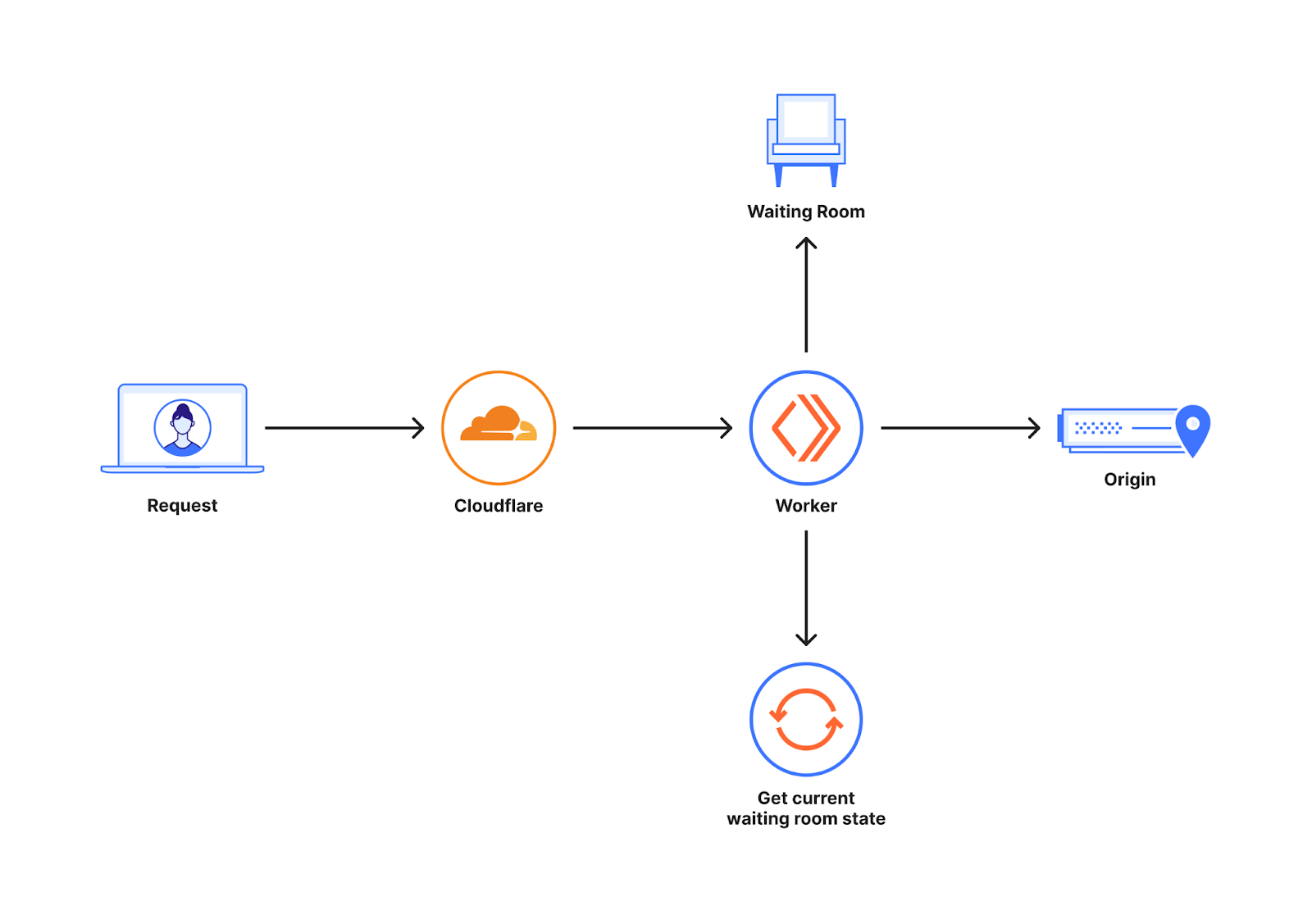
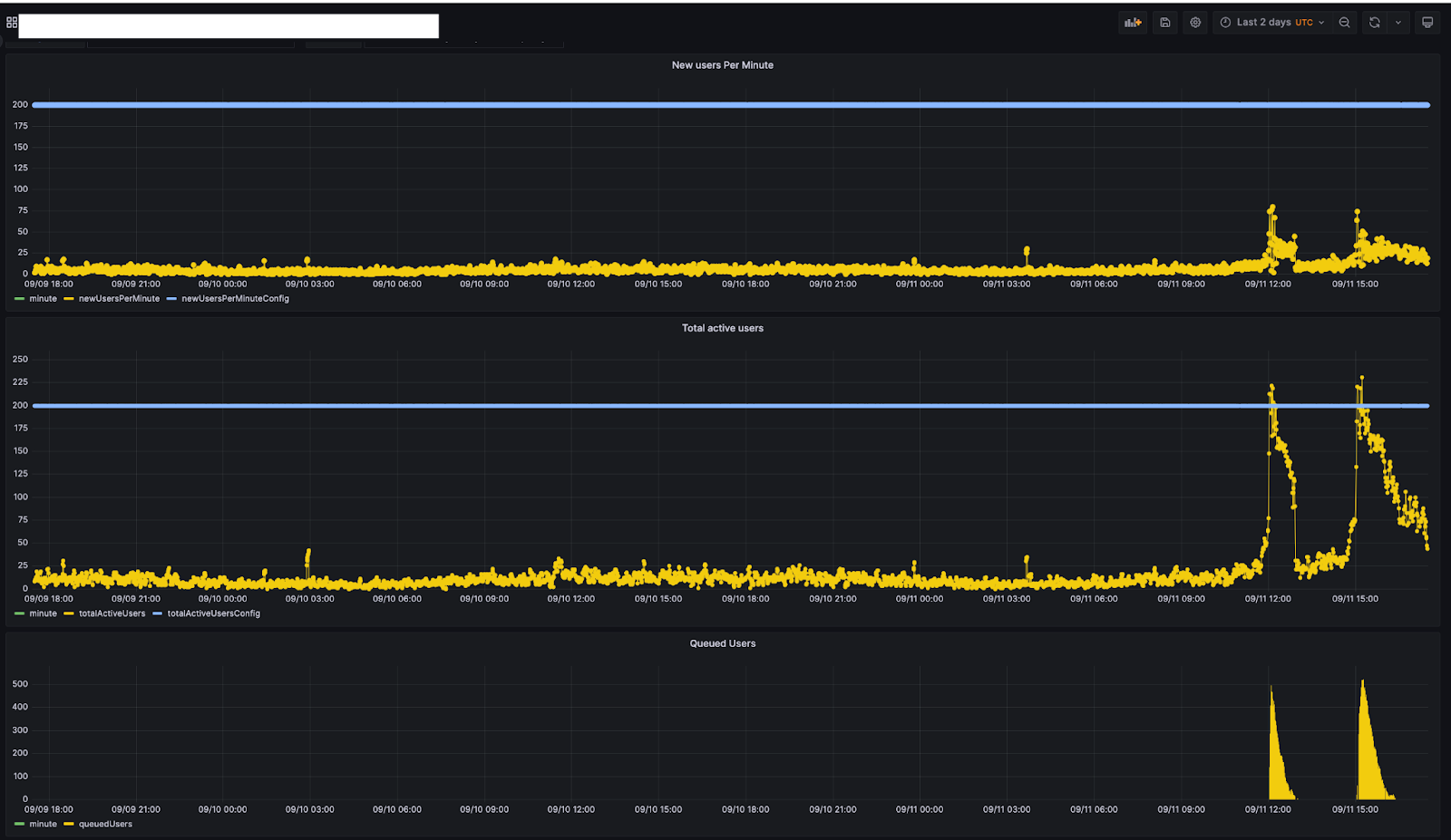
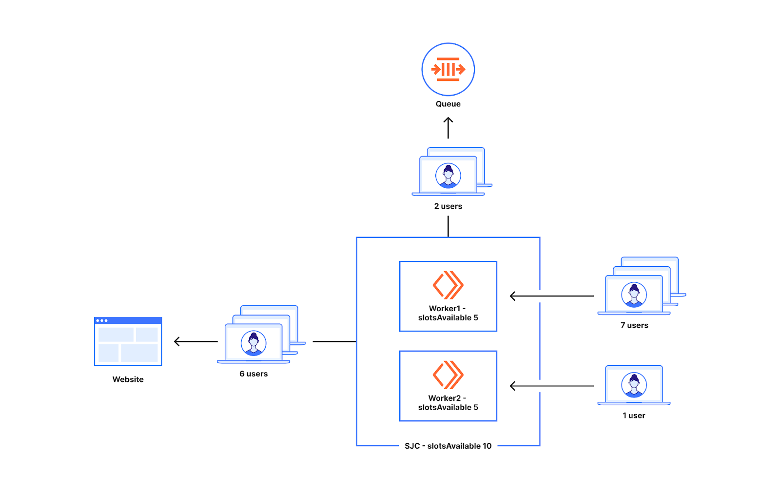
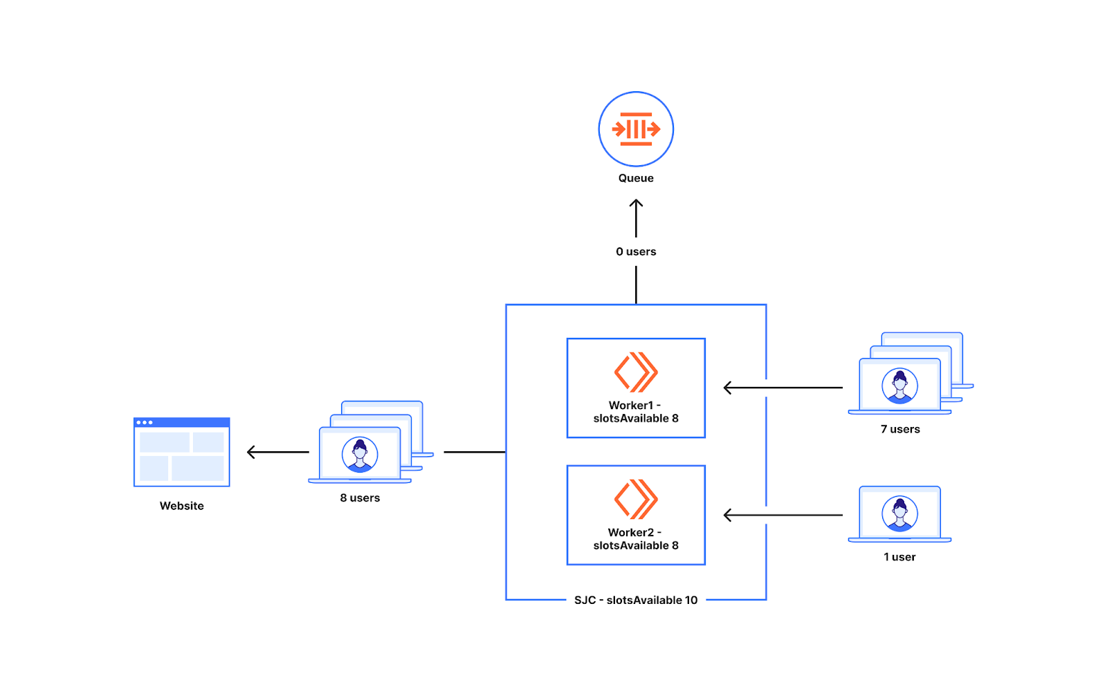


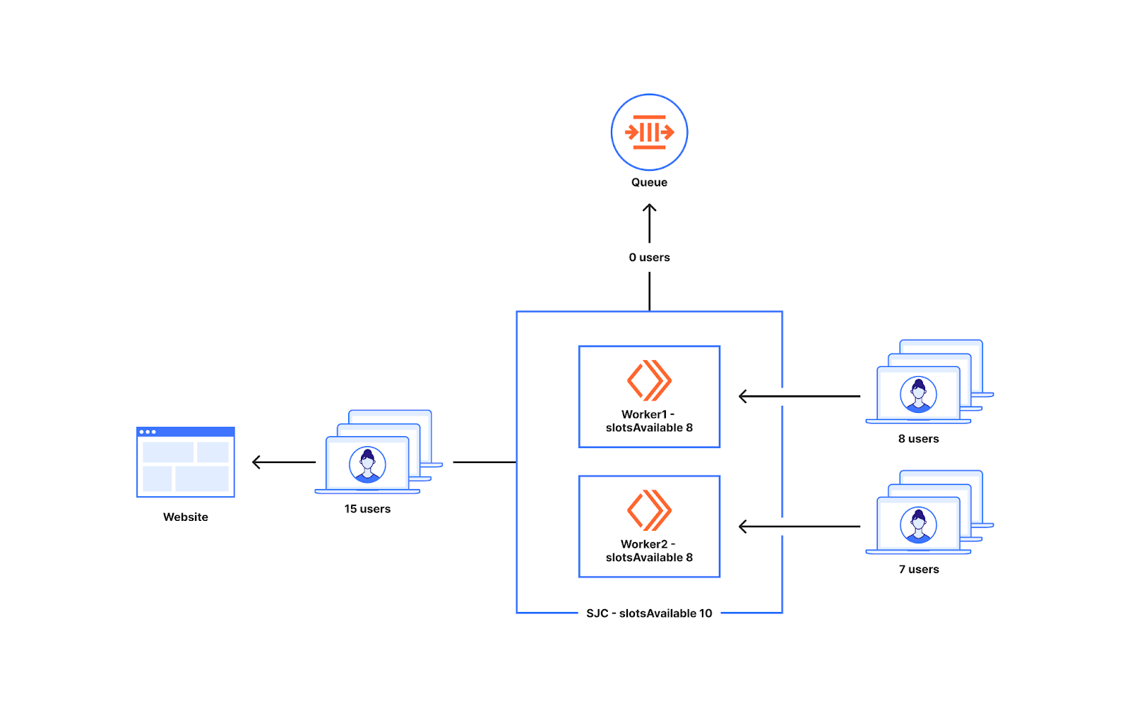
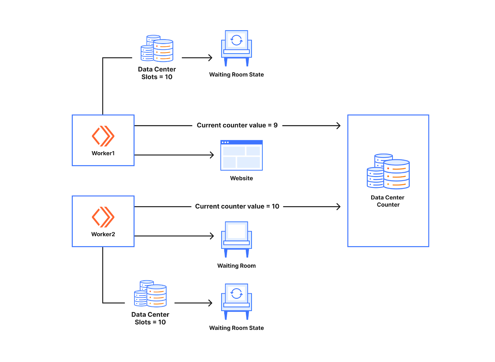
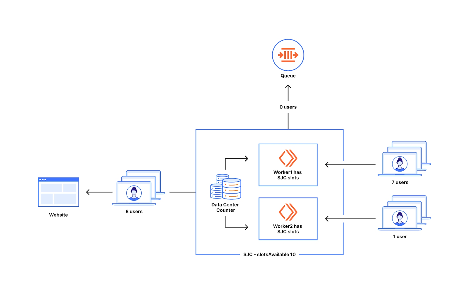
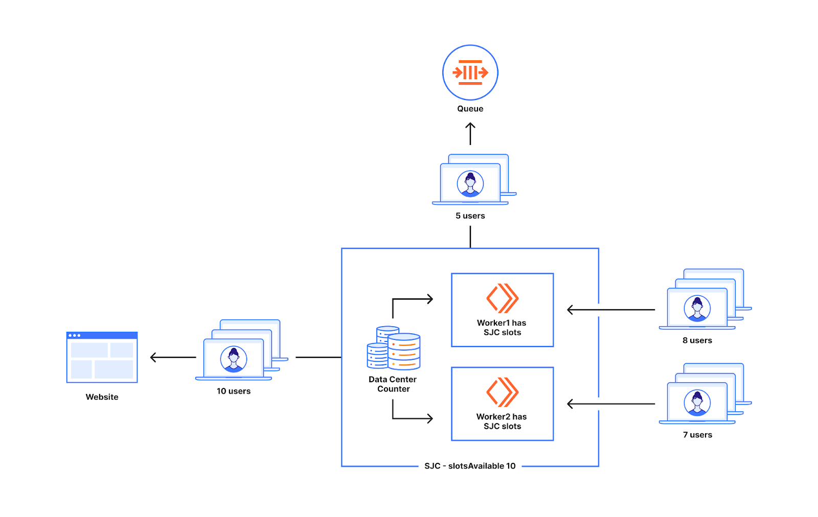
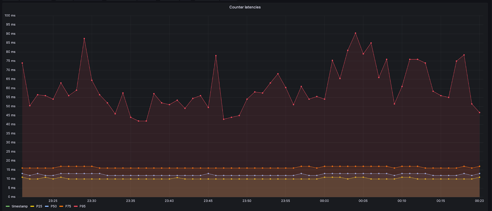
 В Село Марково пак недоволстват хората, че нямало рейс.


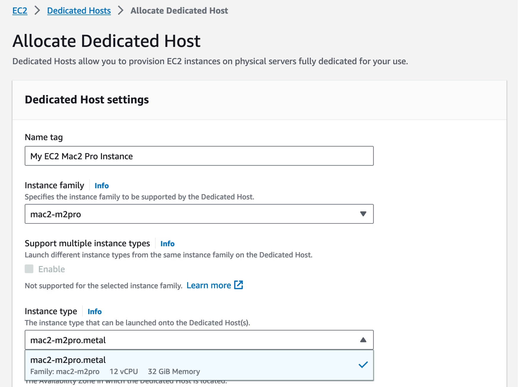
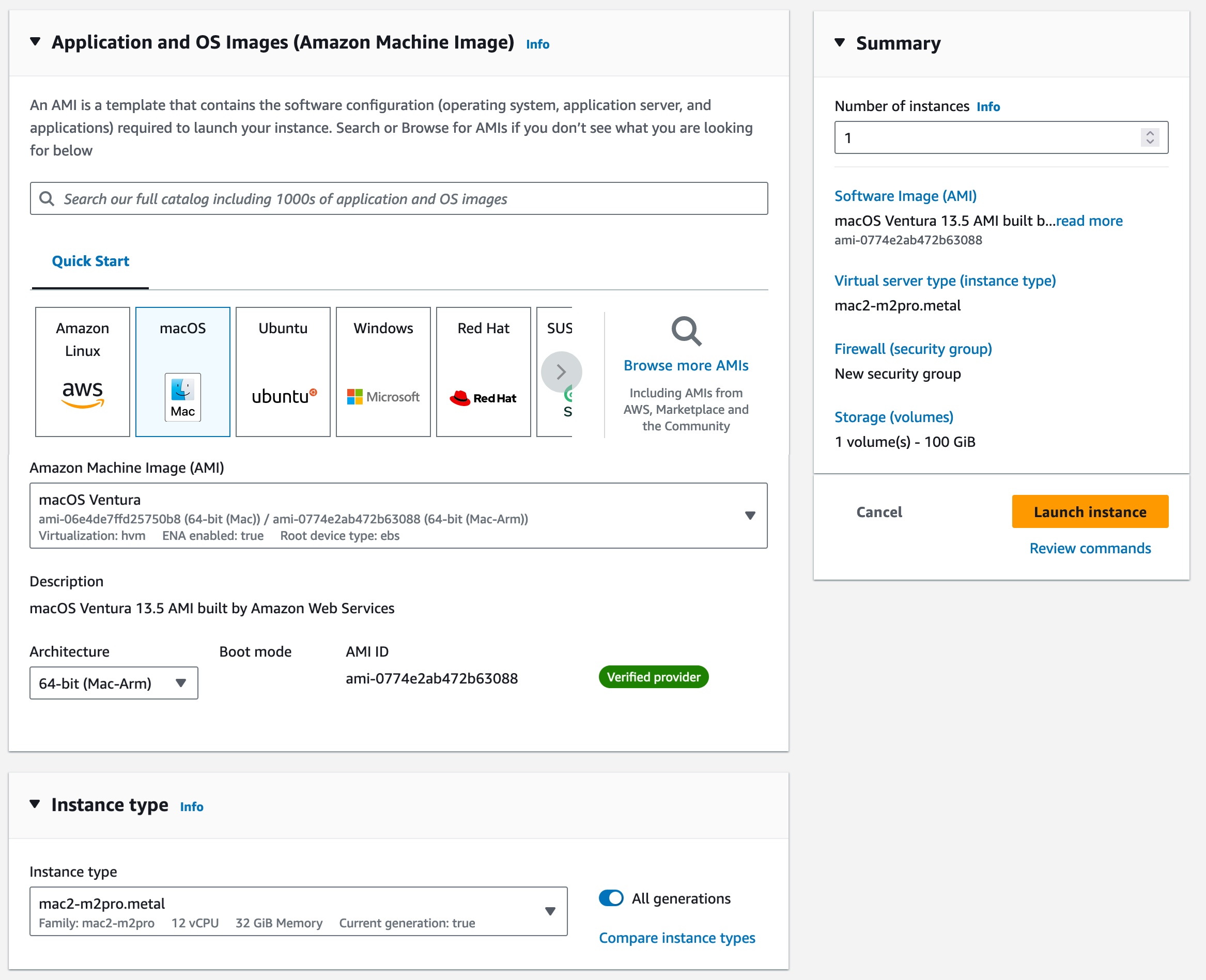
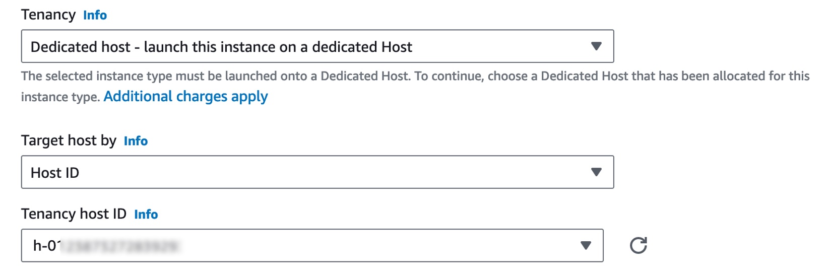


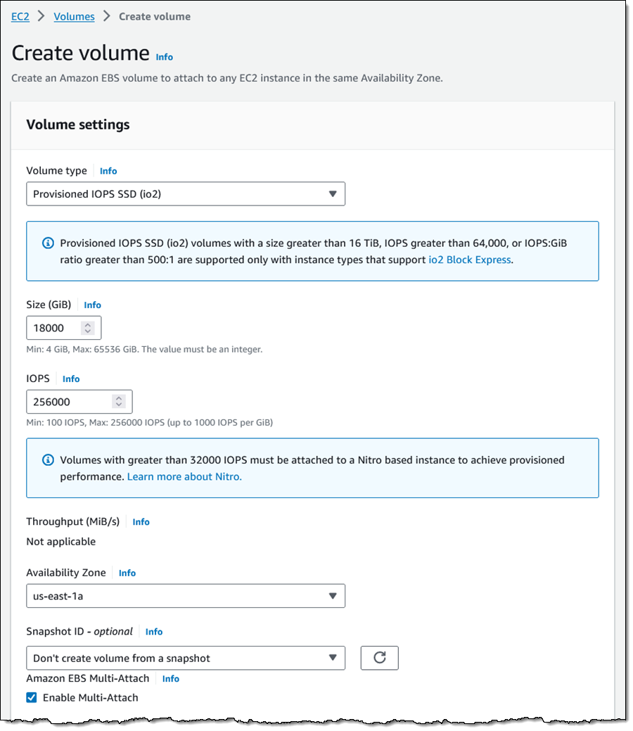
 RamC Venkatasamy is a Solutions Architect based in Bloomington, Illinois. He helps AWS Strategic customers transform their businesses in the cloud. With a fervent enthusiasm for Serverless, Event-Driven Architecture and GenAI.


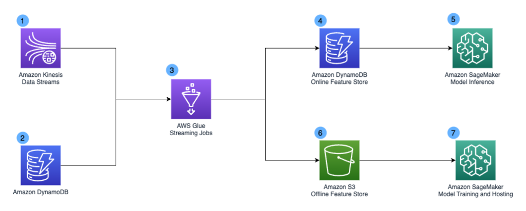
 Khandu Shinde is a Staff Engineer focused on Big Data Platforms and Solutions for Chime. He helps to make the platform scalable for Chime’s business needs with architectural direction and vision. He’s based in San Francisco where he plays cricket and watches movies.
 Edward Paget is a Software Engineer working on building Chime’s capabilities to mitigate risk to ensure our members’ financial peace of mind. He enjoys being at the intersection of big data and programming language theory. He’s based in Chicago where he spends his time running along the lake shore.
 Dylan Qu is a Specialist Solutions Architect focused on Big Data & Analytics with Amazon Web Services. He helps customers architect and build highly scalable, performant, and secure cloud-based solutions on AWS.