Post Syndicated from BeardedTinker original https://www.youtube.com/watch?v=NOML3aBkInA
AI 101: GPU vs. TPU vs. NPU
Post Syndicated from Stephanie Doyle original https://www.backblaze.com/blog/ai-101-gpu-vs-tpu-vs-npu/

This article is part of an ongoing content arc about artificial intelligence (AI). The first article in the series is AI 101: How Cognitive Science and Computer Processors Create Artificial Intelligence. Stay tuned for the rest of the series, and feel free to suggest other articles you’d like to see on this content in the comments.
It’s no secret that artificial intelligence (AI) is driving innovation, particularly when it comes to processing data at scale. Machine learning (ML) and deep learning (DL) algorithms, designed to solve complex problems and self-learn over time, are exploding the possibilities of what computers are capable of.
It’s no secret that artificial intelligence (AI) is driving innovation, particularly when it comes to processing data at scale. Machine learning (ML) and deep learning (DL) algorithms, designed to solve complex problems and self-learn over time, are exploding the possibilities of what computers are capable of.
As the problems we ask computers to solve get more complex, there’s also an unavoidable, explosive growth in the number of processes they run. This growth has led to the rise of specialized processors and a whole host of new acronyms.
Joining the ranks of central processing units (CPUs), which you may already be familiar with, are neural processing units (NPUs), graphics processing units (GPUs), and tensile processing units (TPUs).
So, let’s dig in to understand how some of these specialized processors work, and how they’re different from each other. If you’re still with me after that, stick around for an IT history lesson. I’ll get into some of the more technical concepts about the combination of hardware and software developments in the last 100 or so years.
Central Processing Unit (CPU): The OG
Think of the CPU as the general of your computer. There are two main parts of a CPU, an arithmetic-logic unit (ALU) and a control unit. An ALU allows arithmetic (add, subtract, etc.) and logic (AND, OR, NOT, etc.) operations to be carried out. The control unit controls the ALU, memory, and IO functions, which tells them how to respond to the program that’s just been read from the memory.
The best way to track what the CPU does is to think of it as an input/output flow. The CPU will take the request (input), access the memory of the computer for instructions on how to perform that task, delegate the execution to either its own ALUs or another specialized processor, take all that data back into its control unit, then take a single, unified action (output).
For a visual, this is the the circuitry map for an ALU from 1970:

But, more importantly, here’s a logic map about what a CPU does:

CPUs have gotten more powerful over the years as we’ve moved from single-core processors to multicore processors. Basically, there are several ALUs executing tasks that are being managed by the CPU’s control unit, and they perform tasks in parallel. That means that it works well in combination with specialized AI processors like GPUs.
The Rise of Specialized Processors
When a computer is given a task, the first thing the processor has to do is communicate with the memory, including program memory (ROM)—designed for more fixed tasks like startup—and data memory (RAM)—designed for things that change more often like loading applications, editing a document, and browsing the internet. The thing that allows these elements to talk is called the bus, and it can only access one of the two types of memory at one time.
In the past, processors ran more slowly than memory access, but that’s changed as processors have gotten more sophisticated. Now, when CPUs are asked to do a bunch of processes on large amounts of data, the CPU ends up waiting for memory access because of traffic on the bus. In addition to slower processing, it also uses a ton of energy. Folks in computing call this the Von Neumann bottleneck, and as compute tasks like those for AI have become more complex, we’ve had to work out ways to solve this problem.
One option is to create chips that are optimized to specific tasks. Specialized chips are designed to solve the processing difficulties machine learning algorithms present to CPUs. In the race to create the best AI processor, big players like Google, IBM, Microsoft, and Nvidia have solved this with specialized processors that can execute more logical queries (and thus more complex logic). They achieve this in a few different ways. So, let’s talk about what that looks like: What are GPUs, TPUs, and NPUs?
Graphics Processing Unit (GPU)
GPUs started out as specialized graphics processors and are often conflated with graphics cards (which have a bit more hardware to them). GPUs were designed to support massive amounts of parallel processing, and they work in tandem with CPUs, either fully integrated on the main motherboard, or, for heavier loads, on their own dedicated piece of hardware. They also use a ton of energy and thus generate heat.
GPUs have long been used in gaming, and it wasn’t until the 2000s that folks started using them for general computing—thanks to Nvidia. Nvidia certainly designs chips, of course, but they also introduced a proprietary platform called CUDA that allows programmers to have direct access to a GPU’s virtual instruction set and parallel computational elements. This means that you can set up compute kernels, or clusters of processors that work together and are ideally suited to specific tasks, without taxing the rest of your resources. Here’s a great diagram that shows the workflow:

This made GPUs wildly applicable for machine learning tasks, and they benefited from the fact that they leveraged existing, well-known processes. What we mean by that is: oftentimes when you’re researching solutions, the solution that wins is not always the “best” one based on pure execution. If you’re introducing something that has to (for example) fundamentally change consumer behavior, or that requires everyone to relearn a skill, you’re going to have resistance to adoption. So, GPUs playing nice with existing systems, programming languages, etc. aided wide adoption. They’re not quite plug-and-play, but you get the gist.
As time has gone on, there are now also open source platforms that support GPUs that are supported by heavy-hitting industry players (including Nvidia). The largest of these is OpenCL. And, folks have added tensor cores, which this article does a fabulous job of explaining.
Tensor Processing Unit (TPU)
Great news: the TL:DR of this acronym boils down to: It’s Google’s proprietary AI processor. They started using them in their own data centers in 2015, released them to the public in 2016, and there are some commercially available models. They run on ASICs (hard-etched chips I’ll talk more about later) and Google’s TensorFlow software.
Compared with GPUs, they’re specifically designed to have slightly lower precision, which makes sense given that this makes them more flexible to different types of workloads. I think Google themselves sum it up best:
If it’s raining outside, you probably don’t need to know exactly how many droplets of water are falling per second—you just wonder whether it’s raining lightly or heavily. Similarly, neural network predictions often don’t require the precision of floating point calculations with 32-bit or even 16-bit numbers. With some effort, you may be able to use 8-bit integers to calculate a neural network prediction and still maintain the appropriate level of accuracy.
GPUs, on the other hand, were originally designed for graphics processing and rendering, which relies on each point’s relationship to each other to create a readable image—if you have less accuracy in those points, you amplify that in their vectors, and then you end up with Playstation 2 Spyro instead of Playstation 4 Spyro.

Another important design choice that deviates from CPUs and GPUs is that TPUs are designed around a systolic array. Systolic arrays create a network of processors that are each computing a partial task, then sending it along to the next node until you reach the end of the line. Each node is usually fixed and identical, but the program that runs between them is programmable. It’s called a data processing unit (DPU).
Neural processing unit (NPU)
“NPU” is sometimes used as the category name for all specialized AI processors, but it’s more often specifically applied to those designed for mobile devices. Just for confusion’s sake, note that Samsung also refers to its proprietary chipsets as NPU.
NPUs contain all the necessary information to complete AI processing, and they run on a principle of synaptic weight. Synaptic weight is a term adapted from biology which describes the strength of connection between two neurons. Simply put, in our bodies if two neurons find themselves sharing information more often, the connection between them becomes literally stronger, making it easier for energy to pass between them. At the end of the day, that makes it easier for you to do something. (Wow, the science between habit forming makes a lot more sense now.) Many neural networks mimic this.
When we say AI algorithms learn, this is one of the ways—they track likely possibilities over time, and give more weight to that connected node. The impact is huge when it comes to power consumption. Parallel processing runs each task next to each other, but isn’t great at accounting for the completion of tasks, especially as your architecture scales and processing units might be more separate.
Quick Refresh: Neural Networks and Decision Making in Computers
As we discuss in AI 101, when you’re thinking about the process of making a decision, what you see is that you’re actually making many decisions in a series, and often the things you’re considering before you reach your final decision affect the eventual outcome. Since computers are designed on a strict binary, they’re not “naturally” suited to contextualizing information in order to make better decisions. Neural networks are the solution. They’re based on matrix math, and they look like this:

Basically, you’re asking a computer to have each potential decision check in with all the other possibilities, to weigh the outcome, and to learn from their own experience and sensory information. That all translates to more calculations being run at one time.
Recapping the Key Differences
That was a lot. Here’s a summary:
- Functionality: GPUs were developed for graphics rendering, while TPUs and NPUs are purpose-built for AI/ML workloads.
- Parallelism: GPUs are made for parallel processing, ideal for training complex neural networks. TPUs take this specialization further, focusing on tensor operations to achieve higher speeds and energy efficiencies.
- Customization: TPUs and NPUs are more specialized and customized for AI tasks, while GPUs offer a more general-purpose approach suitable for various compute workloads.
- Use Cases: GPUs are commonly used in data centers and workstations for AI research and training. TPUs are extensively utilized in Google’s cloud infrastructure, and NPUs are prevalent in AI-enabled devices like smartphones and Internet of Things (IoT) gadgets.
- Availability: GPUs are widely available from various manufacturers and accessible to researchers, developers, and hobbyists. TPUs are exclusive to Google Cloud services, and NPUs are integrated into specific devices.
Do the Differences Matter?
The definitions of the different processors start to sound pretty similar after a while. A multicore processor combines multiple ALUs under a central control unit. A GPU combines more ALUs under a specialized processor. A TPU combines multiple compute nodes under a DPU, which is analogous to a CPU.
At the end of the day, there’s some nuance about the different design choices between processors, but their impact is truly seen at scale versus at the consumer level. Specialized processors can handle larger datasets more efficiently, which translates to faster processing using less electrical power (though our net power usage may go up as we use AI tools more).
It’s also important to note that these are new and changing terms in a new and changing landscape. Google’s TPU was announced in 2015, just eight years ago. I can’t count the amount of conversations I’ve had that end in a hyperbolic impression of what AI is going to do for/to the world, and that’s largely because people think that there’s no limit to what it is.
But, the innovations that make AI possible were created by real people. (Though, maybe AIs will start coding themselves, who knows.) And, chips that power AI are real things—a piece of silicon that comes from the ground and is processed in a lab. Wrapping our heads around what those physical realities are, what challenges we had to overcome, and how they were solved, can help us understand how we can use these tools more effectively—and do more cool stuff in the future.
Bonus Content: A Bit of a History of the Hardware
Which brings me to our history lesson. In order to more deeply understand our topic today, you have to know a little bit about how computers are physically built. The most fundamental language of computers is binary code, represented as a series of 0s and 1s. Those values correspond to whether a circuit is closed or open, respectively. When a circuit is closed, you cannot push power through it. When it’s open, you can. Transistors regulate current flow, generate electrical signals, and act as a switch or gate. You can connect lots of transistors with circuitry to create an integrated circuit chip.
The combination of open and closed patterns of transistors can be read by your computer. As you add more transistors, you’re able to express more and more numbers in binary code. You can see how this influences the basic foundations of computing in how we measure bits and bytes. Eight transistors store one byte of data: two possibilities for each of the eight transistors, and then every possible combination of those possibilities (2^8) = 256 possible combinations of open/closed gates (bits), so 8 bits = one byte, which can represent any number between 0 and 255.

Improvements in reducing transistor size and increasing transistor density on a single chip has led to improvements in capacity, speed, and power consumption, largely due to our ability to purify semiconductor materials, leverage more sophisticated tools like chemical etching, and improve clean room technology. That all started with the integrated circuit chip.
Integrated circuit chips were invented around 1958, fueled by the discoveries of a few different people who solved different challenges nearly simultaneously. Jack Kilby of Texas Instruments created a hybrid integrated circuit measuring about 7/16” by 1/16” (11.1 mm by 1.6 mm). Robert Noyce (eventual co-founder of Intel) went on to create the first monolithic integrated circuit chip (so, all circuits held on the same chip) and it was around the same size. Here’s a blown-up version of it, held by Noyce:

Note those first chips only held about 60 transistors. Current chips can have billions of transistors etched onto the same microchip, and are even smaller. Here’s an example of what a integrated circuit looks like when it’s exposed:

And, for reference, that’s about this big:

And, that, folks, is one of the reasons you can now have a whole computer in your pocket in the guise of a smartphone. As you can imagine, something the size of a modern laptop or rack-mounted server can combine more of these elements more effectively. Hence, the rise of AI.
One More Acronym: What are FGPAs?
So far, I’ve described fixed, physical points on a chip, but chip performance is also affected by software. Software represents the logic and instructions for how all these things work together. So, when you create a chip, you have two options: you either know what software you’re going to run and create a customized chip that supports that, or you get a chip that acts like a blank slate and can be reprogrammed based on what you need.
The first method is called application-specific integrated circuits (ASIC). However, just like any proprietary build in manufacturing, you need to build them at scale for them to be profitable, and they’re slower to produce. Both CPUs and GPUs typically run on hard-etched chips like this.
Reprogrammable chips are known as field-programmable gate arrays (FPGA). They’re flexible and come with a variety of standard interfaces for developers. That means they’re incredibly valuable for AI applications, and particularly deep learning algorithms—as things rapidly advance, FPGAs can be continuously reprogrammed with multiple functions on the same chip, which lets developers test, iterate, and deliver them to market quickly. This flexibility is most notable in that you can also reprogram things like the input/output (IO) interface, so you can reduce latency and overcome bottlenecks. For that reason, folks will often compare the efficacy of the whole class of ASIC-based processors (CPUs, GPUs, NPUs, TPUs) to FPGAs, which, of course, has also led to hybrid solutions.
Summing It All Up: Chip Technology is Rad
Improvements in materials science and microchip construction laid the foundation for providing the processing capacity required by AI, and big players in the industry (Nvidia, Intel, Google, Microsoft, etc.) have leveraged those chips to create specialized processors.
Simultaneously, software has allowed many processing cores to be networked in order to control and distribute processing loads for increased speeds. All that has led us to the rise in specialized chips that enable the massive demands of AI.
Hopefully you have a better understanding of the different chipsets out there, how they work, and the difference between them. Still have questions? Let us know in the comments.
The post AI 101: GPU vs. TPU vs. NPU appeared first on Backblaze Blog | Cloud Storage & Cloud Backup.
Prime Day 2023 Powered by AWS – All the Numbers
Post Syndicated from Jeff Barr original https://aws.amazon.com/blogs/aws/prime-day-2023-powered-by-aws-all-the-numbers/
As part of my annual tradition to tell you about how AWS makes Prime Day possible, I am happy to be able to share some chart-topping metrics (check out my 2016, 2017, 2019, 2020, 2021, and 2022 posts for a look back).
This year I bought all kinds of stuff for my hobbies including a small drill press, filament for my 3D printer, and irrigation tools. I also bought some very nice Alphablock books for my grandkids. According to our official release, the first day of Prime Day was the single largest sales day ever on Amazon and for independent sellers, with more than 375 million items purchased.
Prime Day by the Numbers
As always, Prime Day was powered by AWS. Here are some of the most interesting and/or mind-blowing metrics:
Amazon Elastic Block Store (Amazon EBS) – The Amazon Prime Day event resulted in an incremental 163 petabytes of EBS storage capacity allocated – generating a peak of 15.35 trillion requests and 764 petabytes of data transfer per day. Compared to the previous year, Amazon increased the peak usage on EBS by only 7% Year-over-Year yet delivered +35% more traffic per day due to efficiency efforts including workload optimization using Amazon Elastic Compute Cloud (Amazon EC2) AWS Graviton-based instances. Here’s a visual comparison:

AWS CloudTrail – AWS CloudTrail processed over 830 billion events in support of Prime Day 2023.
Amazon DynamoDB – DynamoDB powers multiple high-traffic Amazon properties and systems including Alexa, the Amazon.com sites, and all Amazon fulfillment centers. Over the course of Prime Day, these sources made trillions of calls to the DynamoDB API. DynamoDB maintained high availability while delivering single-digit millisecond responses and peaking at 126 million requests per second.
Amazon Aurora – On Prime Day, 5,835 database instances running the PostgreSQL-compatible and MySQL-compatible editions of Amazon Aurora processed 318 billion transactions, stored 2,140 terabytes of data, and transferred 836 terabytes of data.
Amazon Simple Email Service (SES) – Amazon SES sent 56% more emails for Amazon.com during Prime Day 2023 vs. 2022, delivering 99.8% of those emails to customers.
Amazon CloudFront – Amazon CloudFront handled a peak load of over 500 million HTTP requests per minute, for a total of over 1 trillion HTTP requests during Prime Day.
Amazon SQS – During Prime Day, Amazon SQS set a new traffic record by processing 86 million messages per second at peak. This is 22% increase from Prime Day of 2022, where SQS supported 70.5M messages/sec.
Amazon Elastic Compute Cloud (EC2) – During Prime Day 2023, Amazon used tens of millions of normalized AWS Graviton-based Amazon EC2 instances, 2.7x more than in 2022, to power over 2,600 services. By using more Graviton-based instances, Amazon was able to get the compute capacity needed while using up to 60% less energy.
Amazon Pinpoint – Amazon Pinpoint sent tens of millions of SMS messages to customers during Prime Day 2023 with a delivery success rate of 98.3%.
Prepare to Scale
Every year I reiterate the same message: rigorous preparation is key to the success of Prime Day and our other large-scale events. If you are preparing for a similar chart-topping event of your own, I strongly recommend that you take advantage of AWS Infrastructure Event Management (IEM). As part of an IEM engagement, my colleagues will provide you with architectural and operational guidance that will help you to execute your event with confidence!
— Jeff;
Security updates for Wednesday
Post Syndicated from corbet original https://lwn.net/Articles/940103/
Security updates have been issued by Debian (bouncycastle), Fedora (firefox), Red Hat (cjose, curl, iperf3, kernel, kernel-rt, kpatch-patch, libeconf, libxml2, mod_auth_openidc:2.3, openssh, and python-requests), SUSE (firefox, jtidy, libredwg, openssl, salt, SUSE Manager Client Tools, and SUSE Manager Salt Bundle), and Ubuntu (firefox).
Let’s Architect! Resiliency in architectures
Post Syndicated from Luca Mezzalira original https://aws.amazon.com/blogs/architecture/lets-architect-resiliency-in-architectures/
What is “resiliency”, and why does it matter? When we discussed this topic in an early 2022 edition of Let’s Architect!, we referenced the AWS Well-Architected Framework, which defines resilience as having “the capability to recover when stressed by load, accidental or intentional attacks, and failure of any part in the workload’s components.” Businesses rely heavily on the availability and performance of their digital services. Resilience has emerged as critical for any efficiently architected system, which is why it is a fundamental role in ensuring the reliability and availability of workloads hosted on the AWS Cloud platform.
In this newer edition of Let’s Architect!, we share some best practices for putting together resilient architectures, focusing on providing continuous service and avoiding disruptions. Ensuring uninterrupted operations is likely a primary objective when it comes to building a resilient architecture.
Understand resiliency patterns and trade-offs to architect efficiently in the cloud
In this AWS Architecture Blog post, the authors introduce five resilience patterns. Each of these patterns comes with specific strengths and trade-offs, allowing architects to personalize their resilience strategies according to the unique requirements of their applications and business needs. By understanding these patterns and their implications, organizations can design resilient cloud architectures that deliver high availability and efficient recovery from potential disruptions.
Take me to this Architecture Blog post!

Resilience patterns and tradeoffs
Timeouts, retries, and backoff with jitter
Marc Broker discusses the inevitability of failures and the importance of designing systems to withstand them. He highlights three essential tools for building resilience: timeouts, retries, and backoff. By embracing these three techniques, we can create robust systems that maintain high availability in the face of failures. Timeouts, backoff, and jitter are fundamental to spread the traffic coming from clients and avoid overloading your systems. Building resilience is a fundamental aspect of ensuring the reliability and performance of AWS services in the ever-changing and dynamic technological landscape.
Take me to the Amazon Builders’ Library!

The Amazon Builder’s Library is a collection of technical resources produced by engineers at Amazon
Prepare & Protect Your Applications From Disruption With AWS Resilience Hub
The AWS Resilience Hub not only protects businesses from potential downtime risks but also helps them build a robust foundation for their applications, ensuring uninterrupted service delivery to customers and users.
In this AWS Online Tech Talk, led by the Principal Product Manager of AWS Resilience Hub, the importance of a resilience hub to protect mission-critical applications from downtime risks is emphasized. The AWS Resilience Hub is showcased as a centralized platform to define, validate, and track application resilience. The talk includes strategies to avoid disruptions caused by software, infrastructure, or operational issues, plus there’s also a demo demonstrating how to apply these techniques effectively.
If you are interested in delving deeper into the services discussed in the session, AWS Resilience Hub is a valuable resource for monitoring and implementing resilient architectures.
Take me to this AWS Online Tech Talk!

AWS Resilience Hub recommendations
Data resiliency design patterns with AWS
In this re:Invent 2022 session, data resiliency, why it matters to customers, and how you can incorporate it into your application architecture is discussed in depth. This session kicks off with the comprehensive overview of data resiliency, breaking down its core components and illustrating its critical role in modern application development. It, then, covers application data resiliency and protection designs, plus extending from the native data resiliency capabilities of AWS storage through DR solutions using AWS Elastic Disaster Recovery.
Take me to this re:Invent 2022 video!

Asynchronous cross-region replication
See you next time!
Thanks for joining our discussion on architecture resiliency! See you in two weeks when we’ll talk about security on AWS.
To find all the blogs from this series, visit the Let’s Architect! list of content on the AWS Architecture Blog.
Hardening Workers KV
Post Syndicated from Matt Silverlock original http://blog.cloudflare.com/workers-kv-restoring-reliability/

Over the last couple of months, Workers KV has suffered from a series of incidents, culminating in three back-to-back incidents during the week of July 17th, 2023. These incidents have directly impacted customers that rely on KV — and this isn’t good enough.
We’re going to share the work we have done to understand why KV has had such a spate of incidents and, more importantly, share in depth what we’re doing to dramatically improve how we deploy changes to KV going forward.
Workers KV?
Workers KV — or just “KV” — is a key-value service for storing data: specifically, data with high read throughput requirements. It’s especially useful for user configuration, service routing, small assets and/or authentication data.
We use KV extensively inside Cloudflare too, with Cloudflare Access (part of our Zero Trust suite) and Cloudflare Pages being some of our highest profile internal customers. Both teams benefit from KV’s ability to keep regularly accessed key-value pairs close to where they’re accessed, as well its ability to scale out horizontally without any need to become an expert in operating KV.
Given Cloudflare’s extensive use of KV, it wasn’t just external customers impacted. Our own internal teams felt the pain of these incidents, too.
The summary of the post-mortem
Back in June 2023, we announced the move to a new architecture for KV, which is designed to address two major points of customer feedback we’ve had around KV: high latency for infrequently accessed keys (or a key accessed in different regions), and working to ensure the upper bound on KV’s eventual consistency model for writes is 60 seconds — not “mostly 60 seconds”.
At the time of the blog, we’d already been testing this internally, including early access with our community champions and running a small % of production traffic to validate stability and performance expectations beyond what we could emulate within a staging environment.
However, in the weeks between mid-June and culminating in the series of incidents during the week of July 17th, we would continue to increase the volume of new traffic onto the new architecture. When we did this, we would encounter previously unseen problems (many of these customer-impacting) — then immediately roll back, fix bugs, and repeat. Internally, we’d begun to identify that this pattern was becoming unsustainable — each attempt to cut traffic onto the new architecture would surface errors or behaviors we hadn’t seen before and couldn’t immediately explain, and thus we would roll back and assess.
The issues at the root of this series of incidents proved to be significantly challenging to track and observe. Once identified, the two causes themselves proved to be quick to fix, but an (1) observability gap in our error reporting and (2) a mutation to local state that resulted in an unexpected mutation of global state were both hard to observe and reproduce over the days following the customer-facing impact ending.
The detail
One important piece of context to understand before we go into detail on the post-mortem: Workers KV is composed of two separate Workers scripts – internally referred to as the Storage Gateway Worker and SuperCache. SuperCache is an optional path in the Storage Gateway Worker workflow, and is the basis for KV's new (faster) backend (refer to the blog).
Here is a timeline of events:
| Time | Description |
|---|---|
| 2023-07-17 21:52 UTC | Cloudflare observes alerts showing 500 HTTP status codes in the MEL01 data-center (Melbourne, AU) and begins investigating. We also begin to see a small set of customers reporting HTTP 500s being returned via multiple channels. It is not immediately clear if this is a data-center-wide issue or KV specific, as there had not been a recent KV deployment, and the issue directly correlated with three data-centers being brought back online. |
| 2023-07-18 00:09 UTC | We disable the new backend for KV in MEL01 in an attempt to mitigate the issue (noting that there had not been a recent deployment or change to the % of users on the new backend). |
| 2023-07-18 05:42 UTC | Investigating alerts showing 500 HTTP status codes in VIE02 (Vienna, AT) and JNB01 (Johannesburg, SA). |
| 2023-07-18 13:51 UTC | The new backend is disabled globally after seeing issues in VIE02 (Vienna, AT) and JNB01 (Johannesburg, SA) data-centers, similar to MEL01. In both cases, they had also recently come back online after maintenance, but it remained unclear as to why KV was failing. |
| 2023-07-20 19:12 UTC | The new backend is inadvertently re-enabled while deploying the update due to a misconfiguration in a deployment script. |
| 2023-07-20 19:33 UTC | The new backend is (re-) disabled globally as HTTP 500 errors return. |
| 2023-07-20 23:46 UTC | Broken Workers script pipeline deployed as part of gradual rollout due to incorrectly defined pipeline configuration in the deployment script. Metrics begin to report that a subset of traffic is being black-holed. |
| 2023-07-20 23:56 UTC | Broken pipeline rolled back; errors rates return to pre-incident (normal) levels. |
All timestamps referenced are in Coordinated Universal Time (UTC).
We initially observed alerts showing 500 HTTP status codes in the MEL01 data-center (Melbourne, AU) at 21:52 UTC on July 17th, and began investigating. We also received reports from a small set of customers reporting HTTP 500s being returned via multiple channels. This correlated with three data centers being brought back online, and it was not immediately clear if it related to the data centers or was KV-specific — especially given there had not been a recent KV deployment. On 05:42, we began investigating alerts showing 500 HTTP status codes in VIE02 (Vienna) and JNB02 (Johannesburg) data-centers; while both had recently come back online after maintenance, it was still unclear why KV was failing. At 13:51 UTC, we made the decision to disable the new backend globally.
Following the incident on July 18th, we attempted to deploy an allow-list configuration to reduce the scope of impacted accounts. However, while attempting to roll out a change for the Storage Gateway Worker at 19:12 UTC on July 20th, an older configuration was progressed causing the new backend to be enabled again, leading to the third event. As the team worked to fix this and deploy this configuration, they attempted to manually progress the deployment at 23:46 UTC, which resulted in the passing of a malformed configuration value that caused traffic to be sent to an invalid Workers script configuration.
After all deployments and the broken Workers configuration (pipeline) had been rolled back at 23:56 on the 20th July, we spent the following three days working to identify the root cause of the issue. We lacked observability as KV's Worker script (responsible for much of KV's logic) was throwing an unhandled exception very early on in the request handling process. This was further exacerbated by prior work to disable error reporting in a disabled data-center due to the noise generated, which had previously resulted in logs being rate-limited upstream from our service.
This previous mitigation prevented us from capturing meaningful logs from the Worker, including identifying the exception itself, as an uncaught exception terminates request processing. This has raised the priority of improving how unhandled exceptions are reported and surfaced in a Worker (see Recommendations, below, for further details). This issue was exacerbated by the fact that KV's Worker script would fail to re-enter its "healthy" state when a Cloudflare data center was brought back online, as the Worker was mutating an environment variable perceived to be in request scope, but that was in global scope and persisted across requests. This effectively left the Worker “frozen” with the previous, invalid configuration for the affected locations.
Further, the introduction of a new progressive release process for Workers KV, designed to de-risk rollouts (as an action from a prior incident), prolonged the incident. We found a bug in the deployment logic that led to a broader outage due to an incorrectly defined configuration.
This configuration effectively caused us to drop a single-digit % of traffic until it was rolled back 10 minutes later. This code is untested at scale, and we need to spend more time hardening it before using it as the default path in production.
Additionally: although the root cause of the incidents was limited to three Cloudflare data-centers (Melbourne, Vienna, and Johannesburg), traffic across these regions still uses these data centers to route reads and writes to our system of record. Because these three data centers participate in KV’s new backend as regional tiers, a portion of traffic across the Oceania, Europe, and African regions was affected. Only a portion of keys from enrolled namespaces use any given data center as a regional tier in order to limit a single (regional) point of failure, so while traffic across all data centers in the region was impacted, nowhere was all traffic in a given data center affected.
We estimated the affected traffic to be 0.2-0.5% of KV's global traffic (based on our error reporting), however we observed some customers with error rates approaching 20% of their total KV operations. The impact was spread across KV namespaces and keys for customers within the scope of this incident.
Both KV’s high total traffic volume and its role as a critical dependency for many customers amplify the impact of even small error rates. In all cases, once the changes were rolled back, errors returned to normal levels and did not persist.
Thinking about risks in building software
Before we dive into what we’re doing to significantly improve how we build, test, deploy and observe Workers KV going forward, we think there are lessons from the real world that can equally apply to how we improve the safety factor of the software we ship.
In traditional engineering and construction, there is an extremely common procedure known as a “JSEA”, or Job Safety and Environmental Analysis (sometimes just “JSA”). A JSEA is designed to help you iterate through a list of tasks, the potential hazards, and most importantly, the controls that will be applied to prevent those hazards from damaging equipment, injuring people, or worse.
One of the most critical concepts is the “hierarchy of controls” — that is, what controls should be applied to mitigate these hazards. In most practices, these are elimination, substitution, engineering, administration and personal protective equipment. Elimination and substitution are fairly self-explanatory: is there a different way to achieve this goal? Can we eliminate that task completely? Engineering and administration ask us whether there is additional engineering work, such as changing the placement of a panel, or using a horizontal boring machine to lay an underground pipe vs. opening up a trench that people can fall into.
The last and lowest on the hierarchy, is personal protective equipment (PPE). A hard hat can protect you from severe injury from something falling from above, but it’s a last resort, and it certainly isn’t guaranteed. In engineering practice, any hazard that only lists PPE as a mitigating factor is unsatisfactory: there must be additional controls in place. For example, instead of only wearing a hard hat, we should engineer the floor of scaffolding so that large objects (such as a wrench) cannot fall through in the first place. Further, if we require that all tools are attached to the wearer, then it significantly reduces the chance the tool can be dropped in the first place. These controls ensure that there are multiple degrees of mitigation — defense in depth — before your hard hat has to come into play.
Coming back to software, we can draw parallels between these controls: engineering can be likened to improving automation, gradual rollouts, and detailed metrics. Similarly, personal protective equipment can be likened to code review: useful, but code review cannot be the only thing protecting you from shipping bugs or untested code. Automation with linters, more robust testing, and new metrics are all vastly safer ways of shipping software.
As we spent time assessing where to improve our existing controls and how to put new controls in place to mitigate risks and improve the reliability (safety) of Workers KV, we took a similar approach: eliminating unnecessary changes, engineering more resilience into our codebase, automation, deployment tooling, and only then looking at human processes.
How we plan to get better
Cloudflare is undertaking a larger, more structured review of KV's observability tooling, release infrastructure and processes to mitigate not only the contributing factors to the incidents within this report, but recent incidents related to KV. Critically, we see tooling and automation as the most powerful mechanisms for preventing incidents, with process improvements designed to provide an additional layer of protection. Process improvements alone cannot be the only mitigation.
Specifically, we have identified and prioritized the below efforts as the most important next steps towards meeting our own availability SLOs, and (above all) make KV a service that customers building on Workers can rely on for storing configuration and service data in the hot path of their traffic:
- Substantially improve the existing observability tooling for unhandled exceptions, both for internal teams and customers building on Workers. This is especially critical for high-volume services, where traditional logging alone can be too noisy (and not specific enough) to aid in tracking down these cases. The existing ongoing work to land this will be prioritized further. In the meantime, we have directly addressed the specific uncaught exception with KV's primary Worker script.
- Improve the safety around the mutation of environmental variables in a Worker, which currently operate at "global" (per-isolate) scope, but can appear to be per-request. Mutating an environmental variable in request scope mutates the value for all requests transiting that same isolate (in a given location), which can be unexpected. Changes here will need to take backwards compatibility in mind.
- Continue to expand KV’s test coverage to better address the above issues, in parallel with the aforementioned observability and tooling improvements, as an additional layer of defense. This includes allowing our test infrastructure to simulate traffic from any source data-center, which would have allowed us to more quickly reproduce the issue and identify a root cause.
- Improvements to our release process, including how KV changes and releases are reviewed and approved, going forward. We will enforce a higher level of scrutiny for future changes, and where possible, reduce the number of changes deployed at once. This includes taking on new infrastructure dependencies, which will have a higher bar for both design and testing.
- Additional logging improvements, including sampling, throughout our request handling process to improve troubleshooting & debugging. A significant amount of the challenge related to these incidents was due to the lack of logging around specific requests (especially non-2xx requests)
- Review and, where applicable, improve alerting thresholds surrounding error rates. As mentioned previously in this report, sub-% error rates at a global scale can have severe negative impact on specific users and/or locations: ensuring that errors are caught and not lost in the noise is an ongoing effort.
- Address maturity issues with our progressive deployment tooling for Workers, which is net-new (and will eventually be exposed to customers directly).
This is not an exhaustive list: we're continuing to expand on preventative measures associated with these and other incidents. These changes will not only improve KVs reliability, but other services across Cloudflare that KV relies on, or that rely on KV.
We recognize that KV hasn’t lived up to our customers’ expectations recently. Because we rely on KV so heavily internally, we’ve felt that pain first hand as well. The work to fix the issues that led to this cycle of incidents is already underway. That work will not only improve KV’s reliability but also improve the reliability of any software written on the Cloudflare Workers developer platform, whether by our customers or by ourselves.
Cloudflare Workers database integration with Upstash
Post Syndicated from Joaquin Gimenez original http://blog.cloudflare.com/cloudflare-workers-database-integration-with-upstash/

During Developer Week we announced Database Integrations on Workers a new and seamless way to connect with some of the most popular databases. You select the provider, authorize through an OAuth2 flow and automatically get the right configuration stored as encrypted environment variables to your Worker.
Today we are thrilled to announce that we have been working with Upstash to expand our integrations catalog. We are now offering three new integrations: Upstash Redis, Upstash Kafka and Upstash QStash. These integrations allow our customers to unlock new capabilities on Workers. Providing them with a broader range of options to meet their specific requirements.
Add the integration
We are going to show the setup process using the Upstash Redis integration.
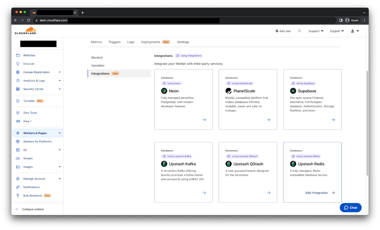
Select your Worker, go to the Settings tab, select the Integrations tab to see all the available integrations.
After selecting the Upstash Redis integration we will get the following page.
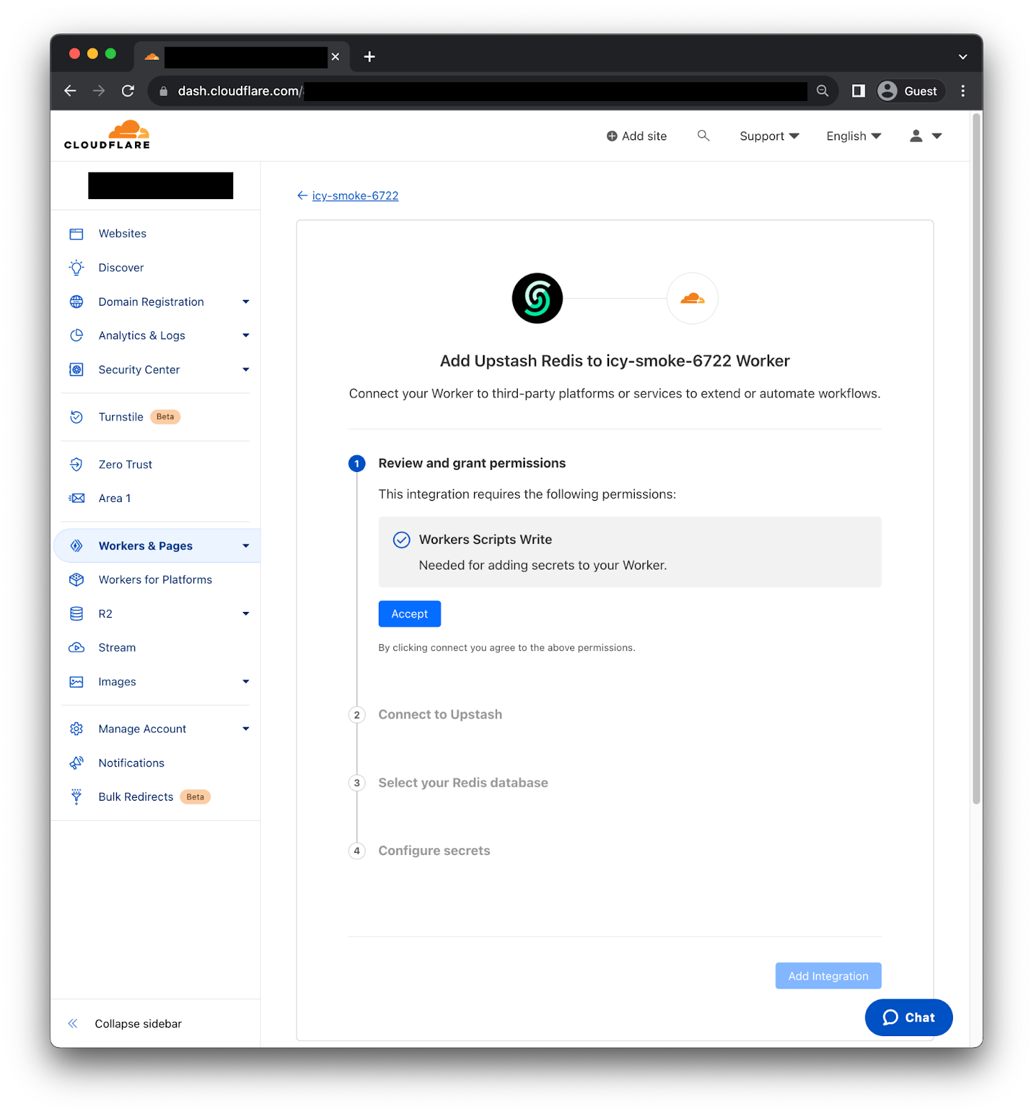
First, you need to review and grant permissions, so the Integration can add secrets to your Worker. Second, we need to connect to Upstash using the OAuth2 flow. Third, select the Redis database we want to use. Then, the Integration will fetch the right information to generate the credentials. Finally, click “Add Integration” and it's done! We can now use the credentials as environment variables on our Worker.
Implementation example
On this occasion we are going to use the CF-IPCountry header to conditionally return a custom greeting message to visitors from Paraguay, United States, Great Britain and Netherlands. While returning a generic message to visitors from other countries.
To begin we are going to load the custom greeting messages using Upstash’s online CLI tool.
➜ set PY "Mba'ẽichapa 🇵🇾"
OK
➜ set US "How are you? 🇺🇸"
OK
➜ set GB "How do you do? 🇬🇧"
OK
➜ set NL "Hoe gaat het met u? 🇳🇱"
OK
We also need to install @upstash/redis package on our Worker before we upload the following code.
import { Redis } from '@upstash/redis/cloudflare'

export default {
  async fetch(request, env, ctx) {
    const country = request.headers.get("cf-ipcountry");
    const redis = Redis.fromEnv(env);
    if (country) {
      const localizedMessage = await redis.get(country);
      if (localizedMessage) {
        return new Response(localizedMessage);
      }
    }
    return new Response("👋👋 Hello there! 👋👋");
  },
};
Just like that we are returning a localized message from the Redis instance depending on the country which the request originated from. Furthermore, we have a couple ways to improve performance, for write heavy use cases we can use Smart Placement with no replicas, so the Worker code will be executed near the Redis instance provided by Upstash. Otherwise, creating a Global Database on Upstash to have multiple read replicas across regions will help.
Try it now
Upstash Redis, Kafka and QStash are now available for all users! Stay tuned for more updates as we continue to expand our Database Integrations catalog.
How we build containerized services at GitHub using GitHub
Post Syndicated from MV Karan original https://github.blog/2023-08-02-how-we-build-containerized-services-at-github-using-github/
The developer experience engineering team at GitHub works on creating safe, delightful, and inclusive solutions for GitHub engineers to efficiently code, ship, and operate software–setting an example for the world on how to build software with GitHub. To achieve this we provide our developers with a paved path–a comprehensive suite of automated tools and applications to streamline our runtime platforms, deployment, and hosting that helps power some of the microservices on the GitHub.com platform and many internal tools. Let’s take a deeper look at how one of our main paved paths works.
Our development ecosystem
GitHub’s main paved path covers everything that’s needed for running software–creating, deploying, scaling, debugging, and running applications. It is an ecosystem of tools like Kubernetes, Docker, load balancers, and many custom apps that work together to create a cohesive experience for our engineers. It isn’t just infrastructure and isn’t just Kubernetes. Kubernetes is our base layer, and the paved path is a mix of conventions, tools, and settings built on top of it.
The kind of services that we typically run using the paved path include web apps, computation pipelines, batch processors, and monitoring systems.
Kubernetes, which is the base layer of the paved path, runs in a multi-cluster, multi-region topology.
Benefits of the paved path
There are hundreds of services at GitHub–from a small internal tool to an external API supporting production workloads. For a variety of reasons, it would be inefficient to spin up virtual machines for each service.
- Planning and capacity usage across all services wouldn’t be efficient. We would encounter significant overhead in managing both physical and Kubernetes infrastructure on an ongoing basis.
- Teams would need to build deep expertise in managing their own Kubernetes clusters and would have less time to focus on their application’s unique needs.
- We would have less central visibility of applications.
- Security and compliance would be difficult to standardize and enforce.
With the paved path based on Kubernetes and other runtime apps, we’re instead able to:
- Plan capacity centrally and only for the Kubernetes nodes, so we can optimally use capacity across nodes, as small workloads and large workloads coexist on the same machines.
- Scale rapidly thanks to central capacity planning.
- Easily manage configuration and deployments across services in one central control plane.
- Consistently provide insights into app and deployment performance for individual services.
Onboarding a service
Onboarding a service with the code living in its own repository has been made easy with our ChatOps command service, called Hubot, and GitHub Apps. Service owners can easily generate some basic scaffolding needed to deploy the service by running a command like:
hubot gh-platform app scaffold monalisa-app
A custom GitHub App installed on the service’s GitHub repository will then automatically generate a pull request to add the necessary configurations, which includes:
- A
deployment.yamlfile that defines the service’s deployment environments. - Kubernetes manifests that define
DeploymentandServiceobjects for deploying the service. - A Debian Dockerfile that runs a trivial web server to start off with, which will be used by the Kubernetes manifests.
- Setting up CI builds as GitHub Checks that build the Docker images on every push, and store in a container registry ready for deployment.
Each service that is onboarded to the paved path has its unique Kubernetes namespace that is defined by <app-name>-<environment> and generally has a staging and production environment. This helps separate the workloads of multiple services, and also multiple environments for the same service since each environment gets its own Kubernetes namespace.
Deploying a service
At GitHub, we deploy branches and perform deployments through Hubot ChatOps commands. To deploy a branch named bug-fixes in the monalisa-app repository to the staging environment, a developer would run a ChatOps command like:
hubot deploy monalisa-app/bug-fixes to staging
This triggers a deployment that fetches the Docker image associated with the latest commit in the bug-fixes branch, updates the Kubernetes manifests, and applies those manifests to the clusters in the runtime platform relevant to that environment.
Typically, the Docker image would be deployed to multiple Kubernetes clusters across multiple geographical sites in a region that forms a part of the runtime platform.
To automate pull request merges into the busiest branches and orchestrate the rollout across environments we’re also using merge queue and deployment pipelines, which our engineers can observe and interact with during their deployment.
Securing our services
For any company, the security of the platform itself, along with services running within it, is critical. In addition to our engineering-wide practices, such as requiring two-person reviews on every pull request, we also have Security and Platform teams automating security measures, such as:
- Pre-built Docker images to be used as base images for the Dockerfiles. These base images contain only the necessary packages/dependencies with security updates, a set of installed software that is auditable and curated according to shared needs.
- Build-time and periodic scanning of all packages and running container images, for any vulnerabilities or dependencies needing a patch, powered by our own products for software supply chain security like Dependabot.
- Build time and periodic scanning of GitHub repositories of services for exposed secrets and vulnerabilities, using GitHub’s native security features for advanced security like code scanning and secret scanning.
- Multiple authentication and authorization mechanisms that allow only the relevant individuals to directly access underlying Kubernetes resources.
- Comprehensive telemetry for threat detection.
- Services running in the platform are by default accessible only within GitHub’s internal networks and not exposed on the public internet.
- Branch protection policies are enforced on all production repositories. These policies prevent merging a pull request until designated automated tests pass and the change has been reviewed by a different developer from the one who proposed the change.
Another key aspect of security for an application is how secrets like keys and tokens are managed. At GitHub, we use a centralized secret store to manage secrets. Each service and each environment within the service has its own vault to store secrets. These secrets are then injected into the relevant pods in Kubernetes, which are then exposed to the containers.
The deployment flow, from merge to rollout
The whole deployment process would look something like this:

- A GitHub engineer merges a pull request to a branch in a repository. In the above example, it is the
bug-fixesbranch in themonalisa-apprepository. This repository would also contain the Kubernetes manifest template files for deploying the application. - The pull request merge triggers relevant CI workflows. One of them is a build of the Docker image, which builds the container image based on the Dockerfile specified in the repository, and pushes the image to an internal artifact registry.
- Once all the CI workflows have completed successfully, the engineer initiates a deployment by running a ChatOps command like
hubot deploy monalisa-app/bug-fixes to staging. This triggers a deployment to our environments such asStaging. - The build systems fetch the Kubernetes manifest files from the repository branch, replaces the latest image to be deployed from the artifact registry, injects app secrets from the secret store, and runs some custom operations. At the end of this stage, a ready-to-deploy Kubernetes manifest is available.
- Our deployment systems then apply the Kubernetes manifest to relevant clusters and monitor the rollout status of new changes.
Conclusion
GitHub’s internal paved path helps developers at GitHub focus on building services and delivering value to our users, with minimal focus on the infrastructure. We accomplish this by providing a streamlined path to our GitHub engineers that uses the power of containers and Kubernetes; scalable security, authentication, and authorization mechanisms; and the GitHub.com platform itself.
Want to try some of these for yourself? Learn more about all of GitHub’s features on github.com/features. If you have adopted any of our practices for your own development, give us a shout on Twitter!
The 1925 US Fleet Visit to Australia
Post Syndicated from The History Guy: History Deserves to Be Remembered original https://www.youtube.com/watch?v=qynZqYNaXng
New SEC Rules around Cybersecurity Incident Disclosures
Post Syndicated from Bruce Schneier original https://www.schneier.com/blog/archives/2023/08/new-sec-rules-around-cybersecurity-incident-disclosures.html
The US Securities and Exchange Commission adopted final rules around the disclosure of cybersecurity incidents. There are two basic rules:
- Public companies must “disclose any cybersecurity incident they determine to be material” within four days, with potential delays if there is a national security risk.
- Public companies must “describe their processes, if any, for assessing, identifying, and managing material risks from cybersecurity threats” in their annual filings.
The rules go into effect this December.
In an email newsletter, Melissa Hathaway wrote:
Now that the rule is final, companies have approximately six months to one year to document and operationalize the policies and procedures for the identification and management of cybersecurity (information security/privacy) risks. Continuous assessment of the risk reduction activities should be elevated within an enterprise risk management framework and process. Good governance mechanisms delineate the accountability and responsibility for ensuring successful execution, while actionable, repeatable, meaningful, and time-dependent metrics or key performance indicators (KPI) should be used to reinforce realistic objectives and timelines. Management should assess the competency of the personnel responsible for implementing these policies and be ready to identify these people (by name) in their annual filing.
News article.
Comic for 2023.08.02
Post Syndicated from Explosm.net original https://explosm.net/comics/31323
New Cyanide and Happiness Comic
Unsupervised graph anomaly detection – Catching new fraudulent behaviours
Post Syndicated from Grab Tech original https://engineering.grab.com/graph-anomaly-model
Earlier in this series, we covered the importance of graph networks, graph concepts, graph visualisation, and graph-based fraud detection methods. In this article, we will discuss how to automatically detect new types of fraudulent behaviour and swiftly take action on them.
One of the challenges in fraud detection is that fraudsters are incentivised to always adversarially innovate their way of conducting frauds, i.e., their modus operandi (MO in short). Machine learning models trained using historical data may not be able to pick up new MOs, as they are new patterns that are not available in existing training data. To enhance Grab’s existing security defences and protect our users from these new MOs, we needed a machine learning model that is able to detect them quickly without the need for any label supervision, i.e., an unsupervised learning model rather than the regular supervised learning model.
To address this, we developed an in-house machine learning model for detecting anomalous patterns in graphs, which has led to the discovery of new fraud MOs. Our focus was initially on GrabFood and GrabMart verticals, where we monitored the interactions between consumers and merchants. We modelled these interactions as a bipartite graph (a type of graph for modelling interactions between two groups) and then performed anomaly detection on the graph. Our in-house anomaly detection model was also presented at the International Joint Conference on Neural Networks (IJCNN) 2023, a premier academic conference in the area of neural networks, machine learning, and artificial intelligence.
In this blog, we discuss the model and its application within Grab. For avid audiences that want to read the details of our model, you can access it here. Note that even though we implemented our model for anomaly detection in GrabFood and GrabMart, the model is designed for general purposes and is applicable to interaction graphs between any two groups.
 |
Interaction-Focused Anomaly Detection on Bipartite Node-and-Edge-Attributed Graphs By Rizal Fathony, Jenn Ng, Jia Chen Presented at International Joint Conference on Neural Networks (IJCNN) 2023 |
Before we dive into how our model works, it is important to understand the process of graph construction in our application as the model assumes the availability of the graphs in a standardised format.
Graph construction
We modelled the interactions between consumers and merchants in GrabFood and GrabMart platforms as bipartite graphs (G), where the first group of nodes (U) represents the consumers, the second group of nodes (V) represents the merchants, and the edges (E) connecting them means that the consumers have placed some food/mart orders to the merchants. The graph is also supplied with rich transactional information about the consumers and the merchants in the form of node features (Xu and Xv), as well as order information in the form of edge features (Xe).
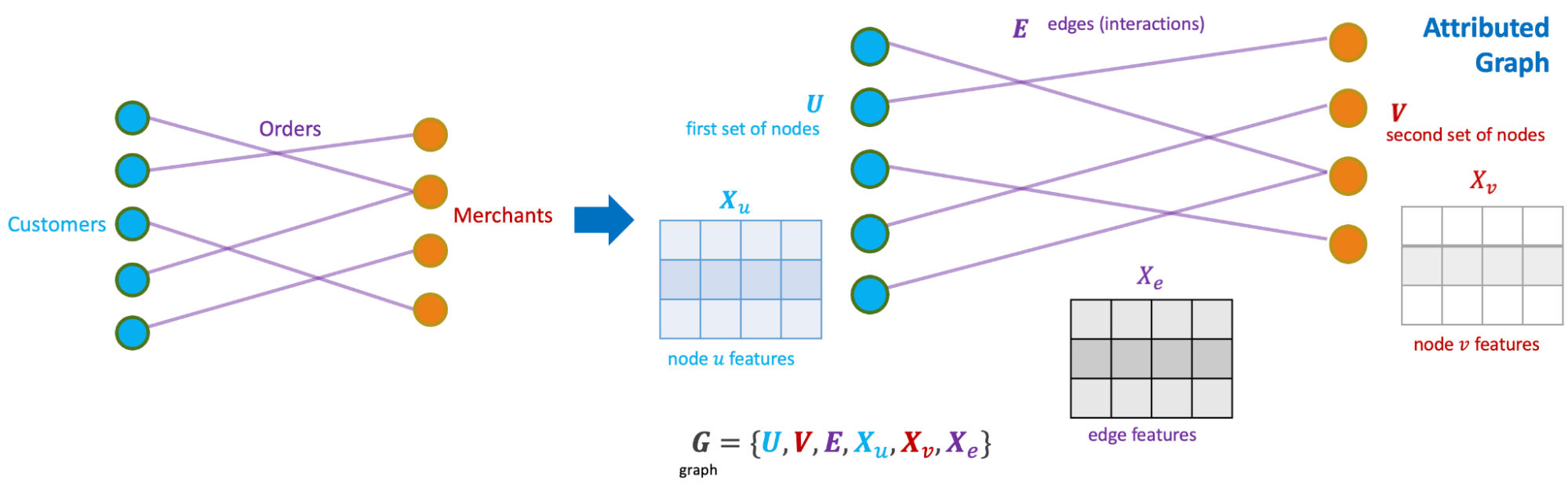
The goal of our anomaly model is to detect anomalous and suspicious behaviours from the consumers or merchants (node-level anomaly detection), as well as anomalous order interactions (edge-level anomaly detection). As mentioned, this detection needs to be done without any label supervision.
Model architecture
We designed our graph anomaly model as a type of autoencoder, with an encoder and two decoders – a feature decoder and a structure decoder. The key feature of our model is that it accepts a bipartite graph with both node and edge attributes as the input. This is important as both node and edge attributes encode essential information for determining if certain behaviours are suspicious. Many previous works on graph anomaly detection only support node attributes. In addition, our model can produce both node and edge level anomaly scores, unlike most of the previous works that produce node-level scores only. We named our model GraphBEAN, which is short for Bipartite Node-and-Edge-Attributed Networks.
From the input, the encoder then processes the attributed bipartite graph into a series of graph convolution layers to produce latent representations for both node groups. Our graph convolution layers produce new representations for each node in both node groups (U and V), as well as for each edge in the graph. Note that the last convolution layer in the encoder only produces the latent representations for nodes, without producing edge representations. The reason for this design is that we only put the latent representations for the active actors, the nodes representing consumers and merchants, but not their interactions.
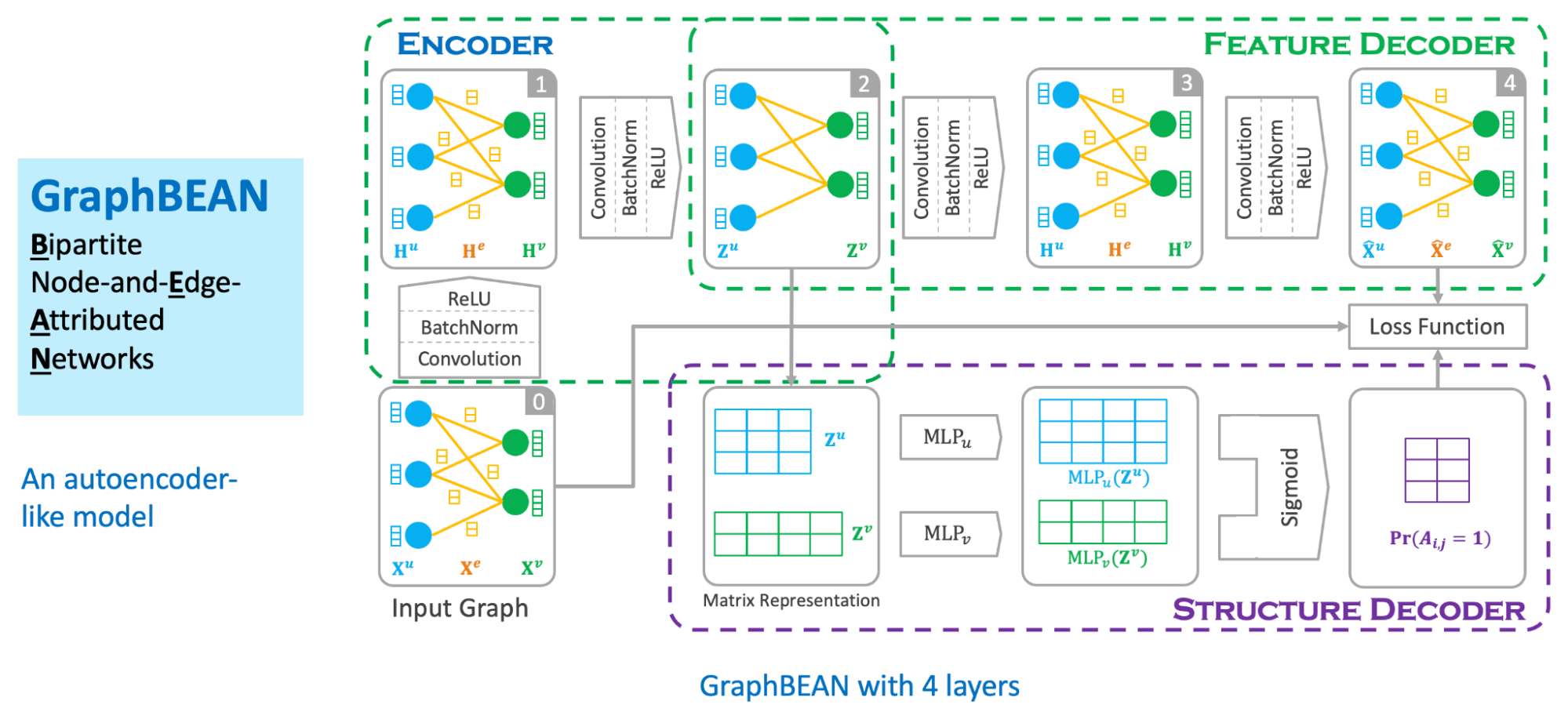
From the nodes’ latent representations, the feature decoder is tasked to reconstruct the original graph with both node and edge attributes via a series of graph convolution layers. As the graph structure is provided by the feature decoder, we task the structure decoder to learn the graph structure by predicting if there exists an edge connecting two nodes. This edge prediction, as well as the graph reconstructed by the feature decoder, are then compared to the original input graph via a reconstruction loss function.
The model is then trained using the bipartite graph constructed from GrabFood and GrabMart transactions. We use a reconstruction-based loss function as the training objective of the model. After the training is completed, we compute the anomaly score of each node and edge in the graph using the trained model.
Anomaly score computation
Our anomaly scores are reconstruction-based. The score design assumes that normal behaviours are common in the dataset and thus, can be easily reconstructed by the model. On the other hand, anomalous behaviours are rare. Therefore the model will have a hard time reconstructing them, hence producing high errors.
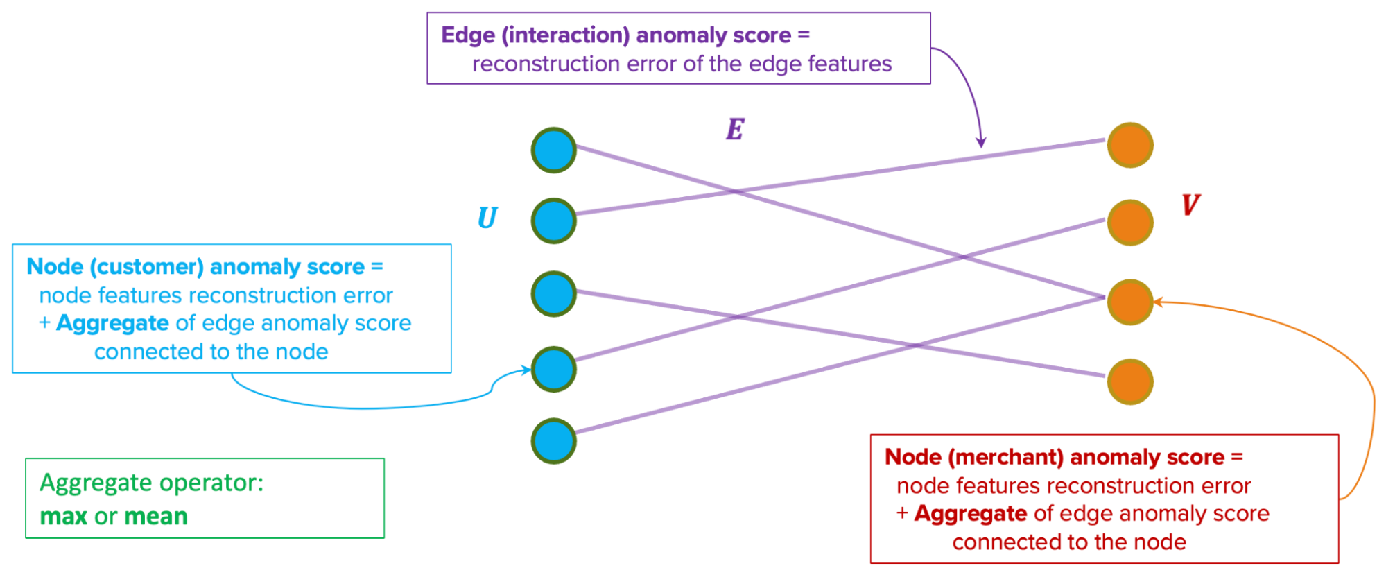
The model produces two types of anomaly scores. First, the edge-level anomaly scores, which are calculated from the edge reconstruction error. Second, the node-level anomaly scores, which are calculated from node reconstruction error plus an aggregate over the edge scores from the edges connected to the node. This aggregate could be a mean or max aggregate.
Actioning system
In our implementation of GraphBEAN within Grab, we designed a full pipeline of anomaly detection and actioning systems. It is a fully-automated system for constructing a bipartite graph from GrabFood and GrabMart transactions, training a GraphBEAN model using the graph, and computing anomaly scores. After computing anomaly scores for all consumers and merchants (node-level), as well as all of their interactions (edge-level), it automatically passes the scores to our actioning system. But before that, it also passes them through a system we call fraud type tagger. This is also a fully-automated heuristic-based system that tags some of the detected anomalies with some fraud tags. The purpose of this tagging is to provide some context in general, like the types of detected anomalies. Some examples of these tags are promo abuse or possible collusion.
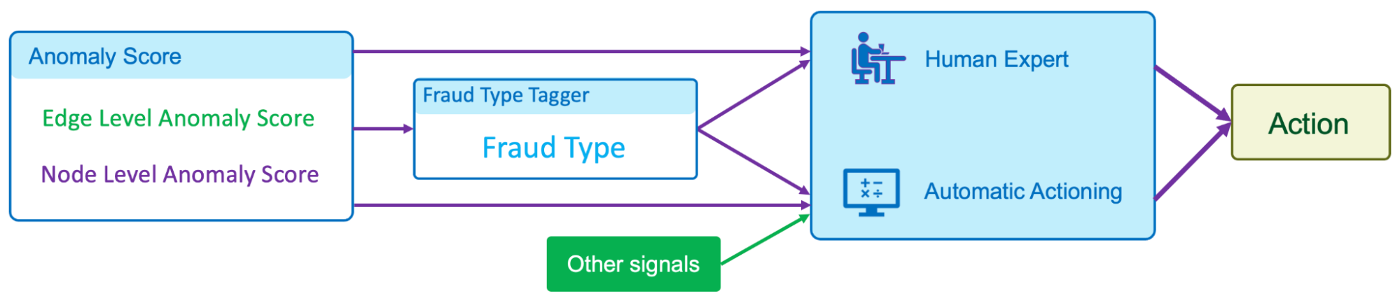
Both the anomaly scores and the fraud type tags are then forwarded to our actioning system. The system consists of two subsystems:
- Human expert actioning system: Our fraud experts analyse the detected anomalies and perform certain actioning on them, like suspending certain transaction features from suspicious merchants.
- Automatic actioning system: Combines the anomaly scores and fraud type tags with other external signals to automatically do actioning on the detected anomalies, like preventing promos from being used by fraudsters or preventing fraudulent transactions from occurring. These actions vary depending on the type of fraud and the scores.
What’s next?
The GraphBEAN model enables the detection of suspicious behaviour on graph data without the need for label supervision. By implementing the model on GrabFood and GrabMart platforms, we learnt that having such a system enables us to quickly identify new types of fraudulent behaviours and then swiftly perform action on them. This also allows us to enhance Grab’s defence against fraudulent activity and actively protect our users.
We are currently working on extending the model into more generic heterogeneous (multi-entity) graphs. In addition, we are also working on implementing it to more use cases within Grab.
Join us
Grab is the leading superapp platform in Southeast Asia, providing everyday services that matter to consumers. More than just a ride-hailing and food delivery app, Grab offers a wide range of on-demand services in the region, including mobility, food, package and grocery delivery services, mobile payments, and financial services across 428 cities in eight countries.
Powered by technology and driven by heart, our mission is to drive Southeast Asia forward by creating economic empowerment for everyone. If this mission speaks to you, join our team today!
How to Coil a Cable
Post Syndicated from xkcd.com original https://xkcd.com/2810/

STH at LTX2023 and LTT Studio in Vancouver BC
Post Syndicated from Patrick Kennedy original https://www.servethehome.com/sth-at-ltx2023-and-ltt-studio-in-vancouver-bc/
Thanks to all of the STH readers and viewers who stopped by to say hi in Vancouver, BC for LTX Expo 2023 this week. Here is a quick recap
The post STH at LTX2023 and LTT Studio in Vancouver BC appeared first on ServeTheHome.
Amazon Kinesis Data Streams on-demand capacity mode now scales up to 1 GB/second ingest capacity
Post Syndicated from Nihar Sheth original https://aws.amazon.com/blogs/big-data/amazon-kinesis-data-streams-on-demand-capacity-mode-now-scales-up-to-1-gb-second-ingest-capacity/
Amazon Kinesis Data Streams is a serverless data streaming service that makes it easy to capture, process, and store streaming data at any scale. As customers collect and stream more types of data, they have asked for simpler, elastic data streams that can handle variable and unpredictable data traffic. In November 2021, Amazon Web Services launched the on-demand capacity mode for Kinesis Data Streams, which is capable of serving gigabytes of write and read throughput per minute and helps reduce the operational pain point of manually updating data stream capacity. You can create a new on-demand data stream or convert an existing data stream to on-demand mode with a single click and never have to provision and manage servers, storage, or throughput. By default, on-demand capacity mode can automatically scale up to 200 MB/s of write throughput.
We were encouraged by customers’ adoption of on-demand capacity mode, but as customers scaled their workloads, some ran into the 200 MB/s data ingestion limit and asked for a solution. The team worked backward from customer feedback to raise that limit. As of March 2023, Kinesis Data Streams supports an increased on-demand write throughput limit to 1 GB/s, a five-times increase from the current limit of 200 MB/s. It’s like having a truly serverless and elastic data streaming service that works for all your use cases. If you require an increase in capacity, you can contact AWS Support to enable on-demand streams to scale up to 1 GB/s write throughput for each requested account. You pay for throughput consumed rather than for provisioned resources, making it easier to balance costs and performance. Overall, if your data volume can spike unpredictably or you don’t want to manage the number of shards, use on-demand streams.
In this post, we explore how to use Kinesis Data Streams on-demand scaling and best practices to build an efficient data-streaming solution. We discuss different scenarios to avoid write throughput exceptions and scale ingest capacity of Kinesis Data Streams to 1 GB/s in on-demand capacity mode.
Kinesis Data Streams on-demand scaling
A shard serves as a base throughput unit of Kinesis Data Streams. A shard supports 1 MB/s and 1,000 records/s for writes and 2 MB/s for reads. The shard limits ensure predictable performance, making it easy to design and operate a highly reliable data streaming workflow. In on-demand capacity mode, scaling happens at the individual shard level. When the average ingest shard utilization reaches 50% (0.5 MB/s or 500 records/s) in 1 minute, then a shard is split into two shards. If you use random values as a partition key, all shards of the stream will have even traffic, and they will be scaled at the same time. If you use a business-specific key as a partition key, the shards will have uneven traffic. In that scenario, only the shards exceeding an average of 50% utilization will be scaled. Depending upon the number of shards being scaled, it will take up to 15 minutes to split the shards.
When we create a new Kinesis data stream in on-demand capacity mode, by default, Kinesis Data Streams provisions four shards, which provides 4 MB/s write and 8 MB/s read throughput. As the workload ramps up, Kinesis Data Streams increases the number of shards in the stream by monitoring ingest throughput at the shard level. The 4 MB/s default ingest throughput and scaling at shard level in on-demand capacity mode works for most use cases. However, in some specific scenarios, producers may face WriteThroughputExceeded and Rate Exceeded errors, even in on-demand capacity mode. We discuss a few of these scenarios in the following sections and strategies to avoid these errors.
You can create and save record templates and easily send data to Kinesis Data Streams using the Amazon Kinesis Data Generator (KDG) to test the streaming data solution. Alternatively, you can also use the modern load testing framework Locust to run large-scale Kinesis Data Streams load testing. For this post, we use the Locust tool to produce and ingest messages in Kinesis Data Streams for our different use cases.
Scenario 1: A baseline ingest throughput greater than 4 MB/s is needed
To simulate this scenario, run the following AWS Command Line Interface (AWS CLI) command to create the kds-od-default-shards data stream in on-demand capacity mode:
When the kds-od-default-shards data stream is active, run following AWS CLI command to check the number of shards in the data stream:
You can observe that the OpenShardCount value is 4, which means the kds-od-default-shards data stream has an ingest capacity of 4 MB/s.
Next, we use the Locust tool to set the baseline to approximately 25 MB/s records. As displayed in the following Amazon CloudWatch metrics graph, records are getting throttled for the first couple of minutes. Then the kds-od-default-shards data stream scales the number of shards to support 25 MB/s ingest throughput, and records stop getting throttled. You can also rerun the describe-stream-summary AWS CLI command to check the increased number of shards in the data stream.


In a scenario where we know our ingest throughput baseline (25 MB/s) ahead of the time and we don’t want to observe any write throttles, we can create a stream in provisioned mode by specifying the number of shards (30), as shown in the following AWS CLI command (make sure to delete kds-od-default-shards manually from the Kinesis Data Streams console before running the following command):
When the kds-od-default-shards data stream is active, run the following AWS CLI command to convert the data stream’s capacity mode to on-demand:
Next, we send 25 MB/s records to the kds-od-default-shards data stream. As displayed in the following CloudWatch metrics graph, we can observe no write throttles, and the kds-od-default-shards data stream scales the number of shards to handle the increase in ingest volume.


After we send 25 MB/s traffic to the data stream for some time, we can run following AWS CLI command to see that the OpenShardCount value is increased to more than 30 now:
Scenario 2: A significant ingestion spike is expected, which needs ingest throughput greater than the number of shards in the stream
To simulate the scenario, run the following AWS CLI command to create the kds-od-significant-spike data stream in on-demand capacity mode:
As mentioned earlier, by default, the kds-od-significant-spike data stream will have four shards initially because this stream is created in on-demand mode. When the data stream is active, we send 4 MB/s ingest throughput initially and grow the ingest throughput by 30–50% every 5–10 minutes. As displayed in the following CloudWatch metrics graph, the kds-od-significant-spike data stream scales the number of shards to handle the increase in ingest volume.
After approximately 15 minutes, run the following AWS CLI command to find the OpenShardCount value (x) of the kds-od-significant-spike data stream. Then send (x * 2) MB/s ingest throughput in the data stream for 2–3 minutes and reduced ingest throughput to the prior level:
As displayed in the following CloudWatch metrics graph, the records are getting throttled for a few minutes, and then the throttling goes away.


Typically, we face a significant spike scenario when running planned events, such as shopping holidays and product launches. To handle such scenarios, we can proactively change capacity mode from on-demand to provisioned. We can configure the number of shards and pick the ingest capacity we anticipate. After we successfully scale the number of shards to our desired peak capacity in provisioned capacity mode, we can change the capacity mode back to on-demand mode.
Scenario 3: A single partition key starts pushing more than 1 MB/s
Partition keys are used to segregate and route records to different shards of a stream. A partition key is specified by the data producer while adding data to the data stream. For example, let’s assume we have a stream with two shards (shard 1 and shard 2). We can configure the data producer to use two partition keys (key A and key B) so that all records with key A are added to shard 1 and all records with key B are added to shard 2. Choosing a partition key is a very important decision, and we should carefully pick the partition key to ensure equal distribution of records across all the shards of the stream. Messages tied to a single partition key A will be sent to a single shard (shard 1), and at any given instance, messages tied to a single partition key A cannot be distributed across different shards. As mentioned earlier, by default, one shard supports 1 MB/s and 1,000 records/s for writes, and we may end up with an edge case scenario where we are trying to push more than 1 MB/s for a specific partition key. In this scenario, producers will continue to experience throttles and keep retrying indefinitely.
To simulate the scenario, run the following AWS CLI command to create the kds-od-partition-key-throttle data stream in on-demand capacity mode:
As mentioned earlier, by default, the data stream will have four shards initially because this stream is created in on-demand mode. When the data stream is active, we send 1.5 MB/s ingest throughput continuously for the specific partition key A. As displayed in the following CloudWatch metrics graph, we can observe that throttling continues from a single shard even if we are sending 1.5 MB/s ingest throughput, and the kds-od-partition-key-throttle data stream has an overall ingest capacity of 4 MB/s.


To avoid this scenario, we should carefully pick our partition key and ensure that this specific partition key won’t be continuously sending more than 1 MB/s ingest throughput in the data stream.
Scale the ingest capacity of Kinesis Data Streams to 1 GB/s in on-demand capacity mode
To test, we start with approximately 100 MB/s baseline ingest throughput to Kinesis Data Streams in on-demand capacity mode, then we increase ingest throughput rate by 30–50% every 5–10 minutes using Locust load testing tool.
To set up the scenario, first create the kds-od-1gb-stream data stream in provisioned capacity mode and provide a value of 120 for the provisioned shards field:
When the kds-od-1gb-stream data stream is active, switch its capacity mode to on-demand, as shown in the following code. When we change capacity mode from provisioned to on-demand, the shard count (120) remains the same for the data stream even in on-demand capacity mode.
When the kds-od-1gb-stream data stream is in on-demand mode, start the experiment. We send approximately 100 MB/s baseline ingest throughput using the Locust tool and increase 30–50% ingest throughput every 5–10 minutes. As displayed in the following CloudWatch metrics graph, the kds-od-1gb-stream data stream seamlessly scaled to 1 GB/s in on-demand capacity mode. We can also observe that the producers didn’t encounter any write throttles while the data stream was scaling in on-demand capacity mode.

Clean up
To avoid ongoing costs, delete all the data streams that you created as part of this post using the Kinesis Data Streams console.
Conclusion
This post demonstrated the on-demand scaling policy of Kinesis Data Streams with a few scenarios using best practices and showed how to scale ingest capacity to 1 GB/s in on-demand capacity mode. You can have an on-demand write throughput limit that is five times larger than the previous limit of 200 MB/s. Choose on-demand mode if you create new data streams with unknown workloads, have unpredictable application traffic, or prefer not to manage capacity. You can switch between on-demand and provisioned capacity modes two times per 24-hour rolling period. Please leave any feedback in the comments section.
About the Authors
 Nihar Sheth is a Senior Product Manager on the Amazon Kinesis Data Streams team at Amazon Web Services. He is passionate about developing intuitive product experiences that solve complex customer problems and enable customers to achieve their business goals.
 Pratik Patel is Sr. Technical Account Manager and streaming analytics specialist. He works with AWS customers and provides ongoing support and technical guidance to help plan and build solutions using best practices and proactively keep customers’ AWS environments operationally healthy.
 Nisha Dekhtawala is a Partner Solutions Architect and data analytics specialist. She works with global consulting partners as their trusted advisor, providing technical guidance and support in building Well-Architected innovative industry solutions.
[$] Challenges for KernelCI
Post Syndicated from jake original https://lwn.net/Articles/939538/
Kernel testing is a perennial topic at Linux-related conferences and the KernelCI project is one of the larger testing
players. It does its own testing but also coordinates with various other
testing systems and aggregates their
results. At the
2023 Embedded
Open Source Summit (EOSS), KernelCI developer Nikolai Kondrashov gave a
presentation on the testing framework, its database, and how others can get
involved in the project. He also had some thoughts on where KernelCI is
falling short of its goals and potential, along with some ideas of ways to
improve it.
THG Podcast: Truth Behind the Legends
Post Syndicated from The History Guy: History Deserves to Be Remembered original https://www.youtube.com/watch?v=M_rk-Q_wsdM
Introducing the first AWS Security Heroes
Post Syndicated from Taylor Jacobsen original https://aws.amazon.com/blogs/aws/introducing-the-first-aws-security-heroes/
The AWS Heroes program recognizes individuals who combine their deeply technical expertise with a passion for helping others to learn more and build faster. Over the years, trends have evolved in how the community develops and deploys solutions built on AWS, which has influenced the creation of specialized Hero categories. Today, we’re thrilled to officially recognize and acknowledge leaders in the security area of focus.
Security is often looked at in terms of impact and not how it enables teams to safely innovate. Our inaugural AWS Security Heroes have shown time and time again that a pragmatic approach, executed with the intent to inform and educate, delivers positive security outcomes. The initial cohort of AWS Security Heroes are experts at the forefront of their field, and share a mission to help others better understand security.
Please join us in welcoming our first AWS Security Heroes!
Chris Farris – Atlanta, USA
 Security Hero Chris Farris has worked in IT since 1994, primarily focused on Linux, networking, and security. For the past eight years, he has been deeply involved in public cloud and public cloud security in media and entertainment, leveraging his expertise to build and evolve cloud security programs at Turner Broadcasting, WarnerMedia, Discovery Communications, and PlayOn! Sports. His current focus is on educating and empowering builders to understand core cloud security concepts, and to enable small and medium sized organizations to better secure and govern in the cloud.
Gerardo Castro – Callao, Perú
 Security Hero Gerardo Castro is a Security Solutions Architect at Caleidos. He likes to write technical posts and talk about cybersecurity on his Medium blog. He also builds and leads videos, podcasts, online classes, and workshops focused on AWS. In addition, Gerardo is a community leader of the AWS UG Security Community in Latin America, and has inspired many people to begin and grow their career in the cloud.
Keisuke Usuda – Chiba, Japan
 Security Hero Keisuke Usuda is a Senior Solution Architect at Classmethod and holds the CISSP certification. He is also a core member of the Japan AWS User Group focused on security (Security-JAWS), and regularly organizes events. Keisuke has a deep affection for AWS security-related managed services, and advocates for the enablement of Amazon GuardDuty across all AWS accounts worldwide.
Ray Lin (Chia-Wei Lin) – Taipei, Taiwan
 Security Hero Ray Lin is an AWS and Security Consultant at iFUS System Consultants Ltd., and excels in building teams and developing new products from zero to one. His primary expertise spans software project management, Agile development, business and system analysis, SaaS product development, architecture design, cybersecurity, DevSecOps, and AI. Ray has also made significant contributions to the AWS community, particularly in cybersecurity and secure architecture design. His commitment to sharing knowledge is evident in his active involvement in the AWS User Group Taiwan.
Shun Yoshie – Yokohama, Japan
 Security Hero Shun Yoshie is a Security Consultant at Nomura Research Institute, Ltd(NRI), and has been a Hero since 2021. He consults on operational design of security in multi-cloud environments, and has been focusing on themes related to multi-cloud, Cloud Native, CNAPP, and Security Observability. Additionally, Shun joined the Japanese AWS User Group (JAWS-UG) in 2013, and he has been running the JAWS-UG Tokyo chapter since 2019.
Teri Radichel – Savannah, USA
 Security Hero Teri Radichel is the CEO of 2nd Sight Lab, a cybersecurity company that offers three services: cloud security training to organizations, penetration tests, and security assessments. She also answers cybersecurity questions for clients on consulting calls scheduled through IANS Research. Teri is the author of the book, “Cybersecurity for Executives in the Age of Cloud,” has been a Hero since 2016, and received the SANS 2017 Difference Makers Award for security innovation. Teri has 13 cybersecurity and pentesting certifications, including the GSE, which required a two-day hands-on in person test to pass at the time she obtained it.
Learn More
If you’d like to learn more about the new Security Hero category or connect with a Hero near you, please visit the AWS Heroes website or browse the AWS Heroes Content Library.
— Taylor
InsightAppSec Advanced Authentication Settings: Token Replacement
Post Syndicated from Shane Queeney original https://blog.rapid7.com/2023/08/01/insightappsec-advanced-authentication-settings-token-replacement/

There are many different ways to use InsightAppSec to authenticate to web apps, but sometimes you need to go deeper into the advanced settings to fully automate your logins, especially with API scanning. Today, we’ll cover one of those advanced settings: Token Replacement.
InsightAppSec Token Replacement can be used to capture and replay Bearer Authentication tokens, JWT Authentication tokens, or any other type of session token.
The token replacement values are under your scan configs in the following location: Custom Options > Advanced > AuthConfig > TokenReplacementList
When you press Add, the following values can be set.
| Name | Description | Possible Values |
| ExtractionTokenLocation | Where the token you want to extract is located. | Request HeaderRequest BodyRequest URLResponse HeadersResponse Body |
| ExtractionTokenRegex | Regex used to extract the token. Anything placed in brackets can be returned in the InjectionTokenRegex using @token@. | Any regex, such as:”token”: ?”([^”]*)”access_token”: ?”([-a-f0-9]+)”[?]sessionId=([^&]*) |
| InjectionTokenLocation | Where the captured token should be injected. | Request URLRequest HeadersRequest Body |
| InjectionTokenRegex | The format in which the token should be sent to the web app. @token@ is replaced with the value captured by ExtractionTokenLocation. | Any string. @token@ is replaced with the captured value. Such as:Authorization: Bearer @token@Authorization: Token @token@&sessionId=@token@ |

Why Token Replacement?
Under Custom Options > HTTP Headers > Extra Header, you can manually pass an authentication token to your web app. While this is the easiest way to set up this form of authentication, unless you generate a token that will not expire, you will have to replace this token every scan. Automating this process using token replacement will save you time and effort in the long run, especially if you have multiple apps you need to generate tokens for.
For this example, we will be using the Rapid7 Hackazon web app. If you want to configure your own Hackazon instance, details around installation and setup can be found here.
Alternatively, there are free public test sites you can use instead, such as this one.
The main difference you’ll encounter when using the Hackazon web app is the API authentication does not have a UI, therefore we must record and pass a traffic file for InsightAppSec to authenticate.
We will use Postman to send the API request to the web app and Burp Suite to record the traffic. You could alternately use the Rapid7 Insight AppSec Toolkit, to record the traffic as well. Here is a video running through setup using the InsightAppSec Toolkit.
The first step is to set up your proxy settings. In Postman, you can go to Settings by clicking the gear icon in the upper right, and then clicking into the proxy settings. We’re going to set the proxy server to “localhost” and change the port to “5000”.

After setting the proxy in Postman, you must set it up in Burp Suite. In Burp, go to the Proxy tab, then click on Proxy Settings. Next, add a proxy listener, specifying port 5000 to match the setting in Postman. Then, set the interface to Loopback Only.

Go back to Postman, add your basic authentication, and then send the traffic. In Burp, click on the HTTP History tab, right click on the captured traffic, then click “Save Item”. Make sure you save the traffic as an xml file.


You can also record the traffic using the Rapid7 Insight AppSec Plugin, or from within the Chrome browser. Instructions for how to do this are located under Traffic Authentication or can be found here.

When recording using the Rapid7 Appsec Plugin, make sure that the recording includes the Bearer Auth or Token in the recorded details.

After recording the login, upload the traffic file to Site Authentication. Make sure you adjust the Logged-In Regex as well to make sure the scan doesn’t fail.


After authenticating to your web app and grabbing the token, the next step is to configure a regex to ensure the token is able to be extracted. There are a wide variety of ways to test the regex, but we will be using https://regex101.com/ for this example.
We will then grab the web app response containing the token info, paste it into the website, and configure a regular expression to ensure only the token is selected. In this use case, the expression “token”: ?”([^”]*) was successful in only highlighting the info we want to extract. We can ensure that only the token is selected in capture Group 1 as that will be returned when we specify @token@ under the InjectionTokenRegex.


Next, we want to configure the TokenReplacementList.
| Name | Value | Reason |
| ExtractionTokenLocation | Response Body | The token appeared in the body after authenticating |
| ExtractionTokenRegex | “token”: ?”([^”]*) | This successfully isolated the auth token |
| InjectionTokenLocation | Request Header | Where the web app is expecting the token |
| InjectionTokenRegex | Authorization: Token @token@ | The header format the web app is expecting |

Make sure you upload the swagger API file. You can either upload the file or point InsightAppSec to the specific URL. You can optionally restrict the scan to just the swagger file for more targeted scanning.

To ensure we were successful, click Download Additional Logs from the Scan Logs page after the scan is complete and open the Operation log file. You are looking for the log entry “[good]: Added imported token from response body”. Once you see this, you know the taken was imported into the scan properly and we were able to use it to log in to the API.
For further testing, you can look in the vulnerability traffic requests to ensure the Authorization: Token header has been passed successfully.


To detect if the token has expired, you can modify the sessionLossRegex and sessionLossHeaderRegex under Authentication > Additional Settings, or by using a CanaryPage if that has been set up. When configured correctly, the token replacement will grab the token again, ensuring we stay logged in to your API.
Further information on configuring Scan Authentication can be found here. When in doubt, please reach out to your web app developers and/or Rapid7 support for assistance.
Empower your Jira data in a data lake with Amazon AppFlow and AWS Glue
Post Syndicated from Tom Romano original https://aws.amazon.com/blogs/big-data/empower-your-jira-data-in-a-data-lake-with-amazon-appflow-and-aws-glue/
In the world of software engineering and development, organizations use project management tools like Atlassian Jira Cloud. Managing projects with Jira leads to rich datasets, which can provide historical and predictive insights about project and development efforts.
Although Jira Cloud provides reporting capability, loading this data into a data lake will facilitate enrichment with other business data, as well as support the use of business intelligence (BI) tools and artificial intelligence (AI) and machine learning (ML) applications. Companies often take a data lake approach to their analytics, bringing data from many different systems into one place to simplify how the analytics are done.
This post shows you how to use Amazon AppFlow and AWS Glue to create a fully automated data ingestion pipeline that will synchronize your Jira data into your data lake. Amazon AppFlow provides software as a service (SaaS) integration with Jira Cloud to load the data into your AWS account. AWS Glue is a serverless data discovery, load, and transformation service that will prepare data for consumption in BI and AI/ML activities. Additionally, this post strives to achieve a low-code and serverless solution for operational efficiency and cost optimization, and the solution supports incremental loading for cost optimization.
Solution overview
This solution uses Amazon AppFlow to retrieve data from the Jira Cloud. The data is synchronized to an Amazon Simple Storage Service (Amazon S3) bucket using an initial full download and subsequent incremental downloads of changes. When new data arrives in the S3 bucket, an AWS Step Functions workflow is triggered that orchestrates extract, transform, and load (ETL) activities using AWS Glue crawlers and AWS Glue DataBrew. The data is then available in the AWS Glue Data Catalog and can be queried by services such as Amazon Athena, Amazon QuickSight, and Amazon Redshift Spectrum. The solution is completely automated and serverless, resulting in low operational overhead. When this setup is complete, your Jira data will be automatically ingested and kept up to date in your data lake!
The following diagram illustrates the solution architecture.
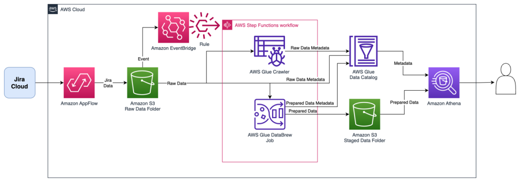
The Step Functions workflow orchestrates the following ETL activities, resulting in two tables:
- An AWS Glue crawler collects all downloads into a single AWS Glue table named
jira_raw. This table is comprised of a mix of full and incremental downloads from Jira, with many versions of the same records representing changes over time. - A DataBrew job prepares the data for reporting by unpacking key-value pairs in the fields, as well as removing depreciated records as they are updated in subsequent change data captures. This reporting-ready data will available in an AWS Glue table named
jira_data.
The following figure shows the Step Functions workflow.
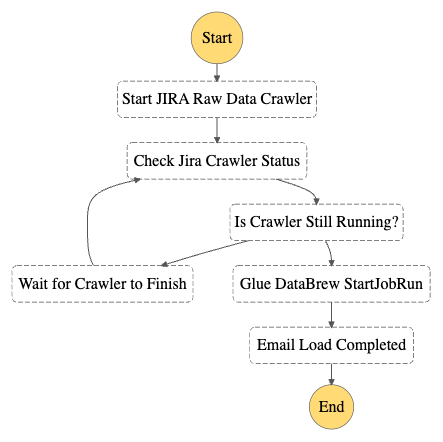
Prerequisites
This solution requires the following:
- Administrative access to your Jira Cloud instance, and an associated Jira Cloud developer account.
- An AWS account and a login with access to the AWS Management Console. Your login will need AWS Identity and Access Management (IAM) permissions to create and access the resources in your AWS account.
- Basic knowledge of AWS and working knowledge of Jira administration.
Configure the Jira Instance
After logging in to your Jira Cloud instance, you establish a Jira project with associated epics and issues to download into a data lake. If you’re starting with a new Jira instance, it helps to have at least one project with a sampling of epics and issues for the initial data download, because it allows you to create an initial dataset without errors or missing fields. Note that you may have multiple projects as well.
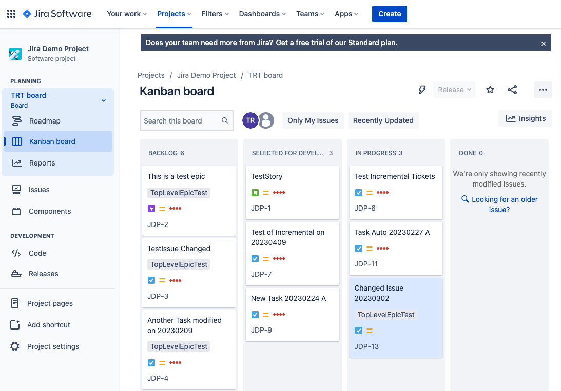
After you have established your Jira project and populated it with epics and issues, ensure you also have access to the Jira developer portal. In later steps, you use this developer portal to establish authentication and permissions for the Amazon AppFlow connection.
Provision resources with AWS CloudFormation
For the initial setup, you launch an AWS CloudFormation stack to create an S3 bucket to store data, IAM roles for data access, and the AWS Glue crawler and Data Catalog components. Complete the following steps:
- Sign in to your AWS account.
- Click Launch Stack:

- For Stack name, enter a name for the stack (the default is
aws-blog-jira-datalake-with-AppFlow). - For GlueDatabaseName, enter a unique name for the Data Catalog database to hold the Jira data table metadata (the default is
jiralake). - For InitialRunFlag, choose Setup. This mode will scan all data and disable the change data capture (CDC) features of the stack. (Because this is the initial load, the stack needs an initial data load before you configure CDC in later steps.)
- Under Capabilities and transforms, select the acknowledgement check boxes to allow IAM resources to be created within your AWS account.
- Review the parameters and choose Create stack to deploy the CloudFormation stack. This process will take around 5–10 minutes to complete.

- After the stack is deployed, review the Outputs tab for the stack and collect the following values to use when you set up Amazon AppFlow:
- Amazon AppFlow destination bucket (
o01AppFlowBucket) - Amazon AppFlow destination bucket path (
o02AppFlowPath) - Role for Amazon AppFlow Jira connector (
o03AppFlowRole)

- Amazon AppFlow destination bucket (


Configure Jira Cloud
Next, you configure your Jira Cloud instance for access by Amazon AppFlow. For full instructions, refer to Jira Cloud connector for Amazon AppFlow. The following steps summarize these instructions and discuss the specific configuration to enable OAuth in the Jira Cloud:
- Open the Jira developer portal.
- Create the OAuth 2 integration from the developer application console by choosing Create an OAuth 2.0 Integration. This will provide a login mechanism for AppFlow.
- Enable fine-grained permissions. See Recommended scopes for the permission settings to grant AppFlow appropriate access to your Jira instance.
- Add the following permission scopes to your OAuth app:
manage:jira-configurationread:field-configuration:jira
- Under Authorization, set the Call Back URL to return to Amazon AppFlow with the URL
https://us-east-1.console.aws.amazon.com/AppFlow/oauth. - Under Settings, note the client ID and secret to use in later steps to set up authentication from Amazon AppFlow.
Create the Amazon AppFlow Jira Cloud connection
In this step, you configure Amazon AppFlow to run a one-time full data fetch of all your data, establishing the initial data lake:
- On the Amazon AppFlow console, choose Connectors in the navigation pane.
- Search for the Jira Cloud connector.
- Choose Create flow on the connector tile to create the connection to your Jira instance.

- For Flow name, enter a name for the flow (for example,
JiraLakeFlow). - Leave the Data encryption setting as the default.
- Choose Next.

- For Source name, keep the default of Jira Cloud.
- Choose Create new connection under Jira Cloud connection.

- In the Connect to Jira Cloud section, enter the values for Client ID, Client secret, and Jira Cloud Site that you collected earlier. This provides the authentication from AppFlow to Jira Cloud.
- For Connection Name, enter a connection name (for example,
JiraLakeCloudConnection). - Choose Connect. You will be prompted to allow your OAuth app to access your Atlassian account to verify authentication.

- In the Authorize App window that pops up, choose Accept.
- With the connection created, return to the Configure flow section on the Amazon AppFlow console.
- For API version, choose V2 to use the latest Jira query API.
- For Jira Cloud object, choose Issue to query and download all issues and associated details.

- For Destination Name in the Destination Details section, choose Amazon S3.
- For Bucket details, choose the S3 bucket name that matches the Amazon AppFlow destination bucket value that you collected from the outputs of the CloudFormation stack.
- Enter the Amazon AppFlow destination bucket path to complete the full S3 path. This will send the Jira data to the S3 bucket created by the CloudFormation script.
- Leave Catalog your data in the AWS Glue Data Catalog unselected. The CloudFormation script uses an AWS Glue crawler to update the Data Catalog in a different manner, grouping all the downloads into a common table, so we disable the update here.
- For File format settings, select Parquet format and select Preserve source data types in Parquet output. Parquet is a columnar format to optimize subsequent querying.
- Select Add a timestamp to the file name for Filename preference. This will allow you to easily find data files downloaded at a specific date and time.

- For now, select Run on Demand for the Flow trigger to run the full load flow manually. You will schedule downloads in a later step when implementing CDC.
- Choose Next.

- On the Map data fields page, select Manually map fields.
- For Source to destination field mapping, choose the drop-down box under Source field name and select Map all fields directly. This will bring down all fields as they are received, because we will instead implement data preparation in later steps.

- Under Partition and aggregation settings, you can set up the partitions in a way that works for your use case. For this example, we use a daily partition, so select Date and time and choose Daily.
- For Aggregation settings, leave it as the default of Don’t aggregate.
- Choose Next.

- On the Add filters page, you can create filters to only download specific data. For this example, you download all the data, so choose Next.
- Review and choose Create flow.
- When the flow is created, choose Run flow to start the initial data seeding. After some time, you should receive a banner indicating the run finished successfully.


Review seed data
At this stage in the process, you now have data in your S3 environment. When new data files are created in the S3 bucket, it will automatically run an AWS Glue crawler to catalog the new data. You can see if it’s complete by reviewing the Step Functions state machine for a Succeeded run status. There is a link to the state machine on the CloudFormation stack’s Resources tab, which will redirect you to the Step Functions state machine.
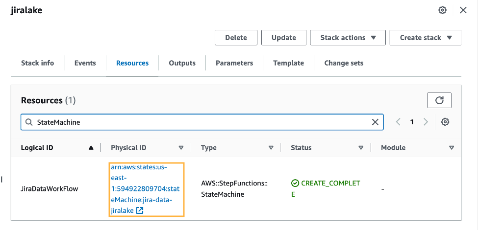
When the state machine is complete, it’s time to review the raw Jira data with Athena. The database is as you specified in the CloudFormation stack (jiralake by default), and the table name is jira_raw. If you kept the default AWS Glue database name of jiralake, the Athena SQL is as follows:
If you explore the data, you’ll notice that most of the data you would want to work with is actually packed into a column called fields. This means the data is not available as columns in your Athena queries, making it harder to select, filter, and sort individual fields within an Athena SQL query. This will be addressed in the next steps.
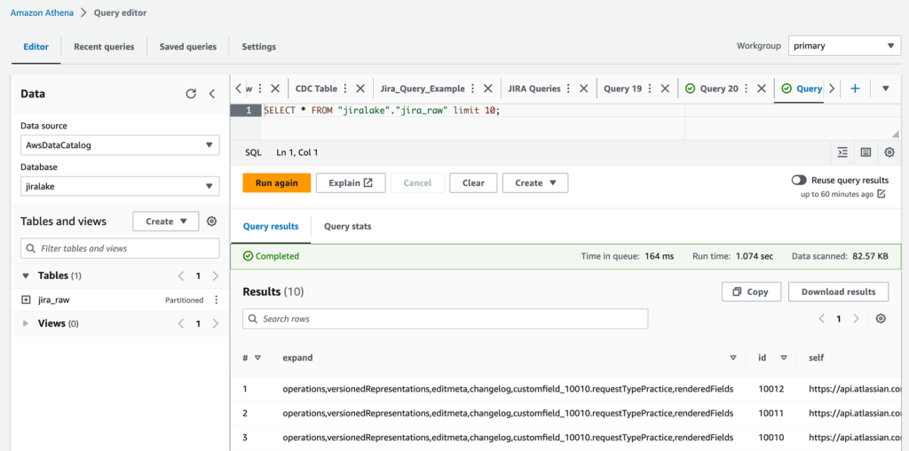
Set up CDC and unpack the fields columns
To add the ongoing CDC and reformat the data for analytics, we introduce a DataBrew job to transform the data and filter to the most recent version of each record as changes come in. You can do this by updating the CloudFormation stack with a flag that includes the CDC and data transformation steps.
- On the AWS CloudFormation console, return to the stack.
- Choose Update.
- Select Use current template and choose Next.

- For SetupOrCDC, choose CDC, then choose Next. This will enable both the CDC steps and the data transformation steps for the Jira data.

- Continue choosing Next until you reach the Review section.
- Select I acknowledge that AWS CloudFormation might create IAM resources, then choose Submit.

- Return to the Amazon AppFlow console and open your flow.
- On the Actions menu, choose Edit flow. We will now edit the flow trigger to run an incremental load on a periodic basis.
- Select Run flow on schedule.
- Configure the desired repeats, as well as start time and date. For this example, we choose Daily for Repeats and enter 1 for the number of days you’ll have the flow trigger. For Starting at, enter 01:00.
- Select Incremental transfer for Transfer mode.
- Choose Updated on the drop-down menu so that changes will be captured based on when the records were updated.
- Choose Save. With these settings in our example, the run will happen nightly at 1:00 AM.


.PNG)
Review the analytics data
When the next incremental load occurs that results in new data, the Step Functions workflow will start the DataBrew job and populate a new staged analytical data table named jira_data in your Data Catalog database. If you don’t want to wait, you can trigger the Step Functions workflow manually.
The DataBrew job performs data transformation and filtering tasks. The job unpacks the key-values from the Jira JSON data and the raw Jira data, resulting in a tabular data schema that facilitates use with BI and AI/ML tools. As Jira items are changed, the changed item’s data is resent, resulting in multiple versions of an item in the raw data feed. The DataBrew job filters the raw data feed so that the resulting data table only contains the most recent version of each item. You could enhance this DataBrew job to further customize the data for your needs, such as renaming the generic Jira custom field names to reflect their business meaning.
When the Step Functions workflow is complete, we can query the data in Athena again using the following query:
You can see that in our transformed jira_data table, the nested JSON fields are broken out into their own columns for each field. You will also notice that we’ve filtered out obsolete records that have been superseded by more recent record updates in later data loads so the data is fresh. If you want to rename custom fields, remove columns, or restructure what comes out of the nested JSON, you can modify the DataBrew recipe to accomplish this. At this point, the data is ready to be used by your analytics tools, such as Amazon QuickSight.
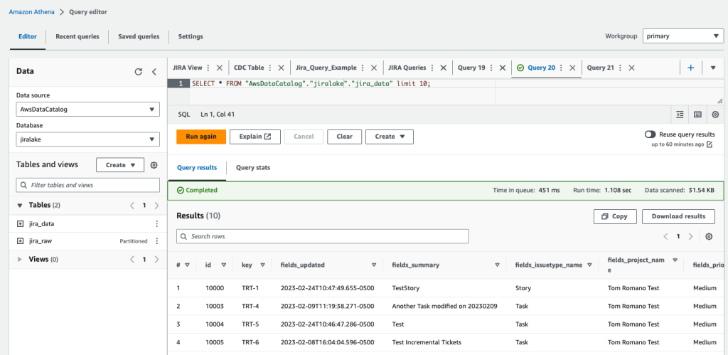
Clean up
If you would like to discontinue this solution, you can remove it with the following steps:
- On the Amazon AppFlow console, deactivate the flow for Jira, and optionally delete it.
- On the Amazon S3 console, select the S3 bucket for the stack, and empty the bucket to delete the existing data.
- On the AWS CloudFormation console, delete the CloudFormation stack that you deployed.
Conclusion
In this post, we created a serverless incremental data load process for Jira that will synchronize data while handling custom fields using Amazon AppFlow, AWS Glue, and Step Functions. The approach uses Amazon AppFlow to incrementally load the data into Amazon S3. We then use AWS Glue and Step Functions to manage the extraction of the Jira custom fields and load them in a format to be queried by analytics services such as Athena, QuickSight, or Redshift Spectrum, or AI/ML services like Amazon SageMaker.
To learn more about AWS Glue and DataBrew, refer to Getting started with AWS Glue DataBrew. With DataBrew, you can take the sample data transformation in this project and customize the output to meet your specific needs. This could include renaming columns, creating additional fields, and more.
To learn more about Amazon AppFlow, refer to Getting started with Amazon AppFlow. Note that Amazon AppFlow supports integrations with many SaaS applications in addition to the Jira Cloud.
To learn more about orchestrating flows with Step Functions, see Create a Serverless Workflow with AWS Step Functions and AWS Lambda. The workflow could be enhanced to load the data into a data warehouse, such as Amazon Redshift, or trigger a refresh of a QuickSight dataset for analytics and reporting.
In future posts, we will cover how to unnest parent-child relationships within the Jira data using Athena and how to visualize the data using QuickSight.
About the Authors
 Tom Romano is a Sr. Solutions Architect for AWS World Wide Public Sector from Tampa, FL, and assists GovTech and EdTech customers as they create new solutions that are cloud native, event driven, and serverless. He is an enthusiastic Python programmer for both application development and data analytics, and is an Analytics Specialist. In his free time, Tom flies remote control model airplanes and enjoys vacationing with his family around Florida and the Caribbean.
 Shane Thompson is a Sr. Solutions Architect based out of San Luis Obispo, California, working with AWS Startups. He works with customers who use AI/ML in their business model and is passionate about democratizing AI/ML so that all customers can benefit from it. In his free time, Shane loves to spend time with his family and travel around the world.