Post Syndicated from Talks at Google original https://www.youtube.com/watch?v=VC69PDlnTp0
SSD 101: How to Upgrade Your Computer With an SSD
Post Syndicated from Andy Klein original https://www.backblaze.com/blog/ssd-upgrade-guide/

Editor’s note: Since it was published in 2019, this post has been updated in 2021 and 2023 with the latest information to help you take advantage of SSDs.
Solid-state drives (SSDs) have become the norm for most laptops and desktops, replacing the older hard disk drives (HDDs) that had been in use for decades previously. If your computer still relies on an HDD, it might be time to consider upgrading to an SSD for improved performance.
Upgrading to an SSD can give your computer a significant speed and responsiveness boost, especially if your machine is more than a few years old. However, before taking the plunge, it’s essential to weigh practical considerations. Let’s take a closer look at SSDs and the factors you should consider.
What Is an SSD?
An SSD is a type of data storage device used in computers and other electronic devices. Unlike traditional HDDs, which use spinning disks and mechanical read/write heads to store and retrieve data, SSDs rely on NAND-based flash memory to store information. This flash memory is similar to the kind used in USB drives and memory cards, but it’s optimized for higher performance and reliability.
Refresher: What Is NAND?
NAND stands for “Not And.” It’s a type of logic gate used in digital circuits, specifically in memory and storage devices. In the context of NAND-based flash memory used in SSDs, the term NAND refers to the electronic structure of the memory cells that store data. The name NAND comes from its logical operation, which is the complement of the AND operation. NAND flash memory is a type of non-volatile storage, meaning it retains data even when the power is turned off, which makes it well-suited for use with things like SSDs and other data storage devices. That’s different from the regular RAM in your computer, which is reset when you turn off or restart the computer.
Compared to HDDs, SSDs are more shock resistant (due to their lack of moving parts) and are less likely to be affected by magnetic fields. They also offer faster data access times, quicker boot-up and application load times, and better overall responsiveness.

For more about the differences between HDDs and SSDs, check out Hard Disk Drive vs. Solid State Drive: What’s the Diff? or our two-part series, HDD vs. SSD: What Does the Future for Storage Hold?.
Why Upgrade to an SSD?
Because of their speed and efficiency, SSDs have become the preferred choice for many computing applications, ranging from laptops and desktops to servers and data centers. They are especially useful in situations where speed and reliability are crucial, such as in gaming, content creation, and tasks involving large data transfers. Despite typically offering less storage capacity compared to HDDs of similar cost, SSD performance benefits often outweigh the storage trade-off, making them a popular choice.
Depending on the task at hand, SSDs can be up to 10 times faster than their HDD counterparts. Replacing your hard drive with an SSD is one of the best things you can do to dramatically improve the performance of your older computer.

Without any moving parts, SSDs operate more quietly, more efficiently, and with fewer breakable things than hard drives that have spinning platters. Read and write speeds for SSDs are much better than hard drives, resulting in noticeably faster operations.
For you, that means less time waiting for stuff to happen. An SSD is worth looking into if you’re frequently seeing a spinning wheel cursor on your computer screen. Modern operating systems rely more on virtual memory management, utilizing temporary swap files that are written to the disk. A faster SSD minimizes the performance impact caused by this process.
If you have just one drive in your laptop or desktop, you could replace an HDD or small SSD with a 1TB SSD for less than $40. For those dealing with substantial amounts of data, concentrating on replacing the drive that houses your operating system and applications can yield a significant speed boost. Put your working data on additional internal or external hard drives, and you’re ready to tackle a mountain of photos, videos, or supersized databases. Just be sure to implement a backup plan to make sure you keep a copy of that data safe on additional local drives, network attached drives, or in the cloud.
Are There Any Reasons Not to Upgrade to an SSD?
If SSDs are so much better than hard drives, why aren’t all drives SSDs? The two biggest reasons are cost and capacity. SSDs are more expensive than hard drives. A 1TB SSD or HDD now cost about the same, $30–$50, with HDDs being slightly less, maybe around $25.
That’s not much of a difference, but as drive capacity gets larger, the cost differential gets increasingly larger. For example, an 8TB HDD drive runs $120–$180, while 8TB SSDs start at around $350. In short, while upgrading the 1TB internal hard drive on your computer to an SSD is cost effective, the same may not be true for replacing larger capacity drives, like those used in external drives, unless the increased speed is worth the increased cost.
Whether your computer can use an SSD is another question. It all depends on the computer’s age and how it was designed. Let’s take a look at that question next.
How Do You Upgrade to an SSD?
Does your computer use a regular off-the-shelf SATA HDD? If so, you can upgrade it with an SSD.
SSDs are compatible with both Macs and PCs. All current Mac laptops come with SSDs. Both iMacs and Mac Pros come with SSDs as well. Around 2010, Apple started moving to only SSD storage on most of its devices. That said, some Mac desktop computers continued to offer the option of both SSD and HDD storage until 2020, a setup they called a Fusion Drive.
Note that as of November 2021, Apple does not offer any Macs with a Fusion Drive. Basically, if you bought your device before 2010 or you have a desktop computer from 2021 or earlier, there’s a chance you may be using an HDD.
Determine Your Disk Type in a Mac
To determine what kind of drive your Mac uses, click on the Apple menu and select About This Mac.
Avoid the pitfall of selecting the Storage tab in the top menu. What you’ll find is that the default name of your drive is “Macintosh HD” which is confusing, given that they’re referring to the internal storage of the computer as a hard drive when (in most cases), your drive is an SSD. While you can find information about your drive on this screen, we prefer the method that provides maximum clarity.
So, on the Overview screen, click System Report. Bonus: You’ll also see what type of processor you have and your macOS version (which will be useful later).

Once there, select the Storage tab, then the volume name you want to identify. You should see a line called Medium Type, which will tell you what kind of drive you have.

Determine Your Disk Type in a PC
To determine your disk type in a Windows PC, first open the Task Manager in Windows:
- Right-click the Start button and click Run. In the Run Command window, type dfrgui and click OK.

- On the next screen, the type of drive will be listed under the Media Type column.

Can I Upgrade to a Better SSD?
Even if your computer already has an SSD, you may be able to upgrade it with a larger, faster SSD model. Besides SATA-based hard drive replacements, some later model PCs can be upgraded with M.2 SSDs, which look more like RAM chips than hard drives.
Some Apple laptops made before 2016 that already shipped with SSDs can be upgraded with larger ones. However, you will need to upgrade to a Mac-specific SSD. Check Other World Computing and Transcend to find ones designed to work. Apple laptop models made after 2016 have SSDs soldered to the motherboard, so you’re stuck with what you have.

How to Install an SSD
If you’re comfortable tinkering with your computer’s guts, upgrading it with an SSD is a pretty common do-it-yourself project. Many companies offer hassle-free plug-and-play SSD replacements. Check out Amazon or NewEgg and you’ll have an embarrassment of riches. The choice is yours: Samsung, SanDisk, Crucial, and Toshiba are all popular SSD makers. There are many others, too.
However, if computer hardware isn’t your forte, it might not be worth the effort to learn from scratch. SSD upgrades are such a common aftermarket improvement most independent computer repair and service specialists will take on the task if you’re willing to pay them. Some throw in a data transfer if you’re lucky, or a skilled negotiator. Ask your friends and colleagues for recommendations. You can also hit up services like Angi to find someone.
If you are DIY inclined, YouTube has tons of walkthroughs like this one for desktop PCs, this one for laptops, and this one aimed at Mac users.

Many SSDs replace 2.5 inch HDDs. Those are the same drives you find in laptop computers and even small desktop models. Have a desktop computer that uses a 3.5 inch hard drive? You may need to use a 2.5 inch to 3.5 inch mounting adapter.
A Word on SSD Compatibility
Beyond the drive size, it’s a good idea to check to see if the SSD you want to buy is compatible with your laptop or desktop, especially if your system is older than a couple of years. Here are articles from Tom’s Hardware and ShareUs which can help with that.
How to Migrate to an SSD
Buying a replacement SSD is the first step. Moving your data onto the SSD is the next step. To achieve this, you need two essential components: cloning software and an external drive case, sled, or enclosure. These tools enable you to connect your SSD to your computer through its USB port or another data transfer interface.
Cloning software creates an exact replica of your internal hard drive’s data. Once this data is successfully migrated to the SSD, you can then insert the new drive into your computer. I prefer to clone a hard drive onto an SSD whenever possible. When executed correctly, a cloned SSD retains its bootable capabilities, providing a true plug-and-play experience. Just copying files between the two drives instead may not copy all the data you need to get the computer to boot with the new drive.
How to Clone a Hard Drive to an SSD
When you buy a new SSD or even a fresh hard drive, it’s unlikely that the operating system you need will be pre-installed. Cloning your existing hard drive fixes that. However, there are instances where this may not be feasible. For example, maybe you’ve installed the SSD in a computer that previously had a bad hard drive. If so, you can do what’s called a clean install and start fresh. Different operating system providers offer distinct guidelines for this procedure. Here’s a link to Microsoft’s clean install procedure, and Apple’s clean install instructions.
As we said at the outset, SSDs tend to come at a higher cost per gigabyte compared to traditional hard drives. You may not be able to afford as large an SSD as your current drive, so make sure your data will fit on your new drive. If it won’t, you might have to pare down first. Additionally, it’s wise to leave some room for expansion. The last thing you want to do is immediately max out your new, fast drive.
Now that you’ve successfully cloned your drive and integrated the SSD into your system, what do you do with the old drive? If it’s still functional, repurposing the external drive chassis utilized during migration is a practical option. It can continue to serve as a standalone external drive or become part of a disk array, such as a network attached storage (NAS) device. You can use it for local back up—something we strongly recommend doing—in addition to using cloud back up like Backblaze. Or, just use it for extra storage needs, like for your photos or music.
Make Sure to Back Up
SSD upgrades are commonplace, but that doesn’t mean things don’t go wrong that can stop you dead in your tracks. If your computer is working fine before the SSD upgrade, make sure you have a complete backup of your computer to restore from in the event something goes wrong.
More Questions About SSDs?
You might enjoy reading other posts in our SSD 101 series.
The post SSD 101: How to Upgrade Your Computer With an SSD appeared first on Backblaze Blog | Cloud Storage & Cloud Backup.
Security updates for Friday
Post Syndicated from jake original https://lwn.net/Articles/942766/
Security updates have been issued by Debian (tryton-server), Fedora (youtube-dl), SUSE (clamav and krb5), and Ubuntu (cjose and fastdds).
Comic for 2023.08.25 – Astronaut
Post Syndicated from Explosm.net original https://explosm.net/comics/astronaut
New Cyanide and Happiness Comic
Using and Managing Security Groups on AWS Snowball Edge devices
Post Syndicated from Macey Neff original https://aws.amazon.com/blogs/compute/using-and-managing-security-groups-on-aws-snowball-edge-devices/
This blog post is written by Jared Novotny & Tareq Rajabi, Specialist Hybrid Edge Solution Architects.
The AWS Snow family of products are purpose-built devices that allow petabyte-scale movement of data from on-premises locations to AWS Regions. Snow devices also enable customers to run Amazon Elastic Compute Cloud (Amazon EC2) instances with Amazon Elastic Block Storage (Amazon EBS), and Amazon Simple Storage Service (Amazon S3) in edge locations.
Security groups are used to protect EC2 instances by controlling ingress and egress traffic. Once a security group is created and associated with an instance, customers can add ingress and egress rules to control data flow. Just like the default VPC in a region, there is a default security group on Snow devices. A default security group is applied when an instance is launched and no other security group is specified. This default security group in a region allows all inbound traffic from network interfaces and instances that are assigned to the same security group, and allows and all outbound traffic. On Snowball Edge, the default security group allows all inbound and outbound traffic.
In this post, we will review the tools and commands required to create, manage and use security groups on the Snowball Edge device.
Some things to keep in mind:
- AWS Snowball Edge is limited to 50 security groups.
- An instance will only have one security group, but each group can have a total of 120 rules. This is comprised of 60 inbound and 60 outbound rules.
- Security groups can only have allow statements to allow network traffic.
- Deny statements aren’t allowed.
- Some commands in the Snowball Edge client (AWS CLI) don’t provide an output.
- AWS CLI commands can use the name or the security group ID.
Prerequisites and tools
Customers must place an order for Snowball Edge from their AWS Console to be able to run the following AWS CLI commands and configure security groups to protect their EC2 instances.
The AWS Snowball Edge client is a standalone terminal application that customers can run on their local servers and workstations to manage and operate their Snowball Edge devices. It supports Windows, Mac, and Linux systems.
AWS OpsHub is a graphical user interface that you can use to manage your AWS Snowball devices. Furthermore, it’s the easiest tool to use to unlock Snowball Edge devices. It can also be used to configure the device, launch instances, manage storage, and provide monitoring.
Customers can download and install the Snowball Edge client and AWS OpsHub from AWS Snowball resources.
Getting Started
To get started, when a Snow device arrives at a customer site, the customer must unlock the device and launch an EC2 instance. This can be done via AWS OpsHub or the AWS Snowball Edge Client. AWS Snow Family of devices support both Virtual Network Interfaces (VNI) and Direct Network interfaces (DNI), customers should review the types of interfaces before deciding which one is best for their use case. Note that security groups are only supported with VNIs, so that is what was used in this post. A post explaining how to use these interfaces should be reviewed before proceeding.
Viewing security group information
Once the AWS Snowball Edge is unlocked, configured, and has an EC2 instance running, we can dig deeper into using security groups to act as a virtual firewall and control incoming and outgoing traffic.
Although the AWS OpsHub tool provides various functionalities for compute and storage operations, it can only be used to view the name of the security group associated to an instance in a Snowball Edge device:

Every other interaction with security groups must be through the AWS CLI.
The following command shows how to easily read the outputs describing the protocols, sources, and destinations. This particular command will show information about the default security group, which allows all inbound and outbound traffic on EC2 instances running on the Snowball Edge.

In the following sections we review the most common commands with examples and outputs.
View (all) existing security groups:
Create new security group:
aws ec2 create-security-group --group-name allow-ssh--description "allow only ssh inbound" --endpoint Http://MySnowIPAddress:8008 --profile SnowballEdge
The output returns a GroupId:
Add port 22 ingress to security group:
aws ec2 authorize-security-group-ingress --group-ids.sg-8f25ee27cee870b4a --protocol tcp --port 22 --cidr 10.100.10.0/24 --endpoint Http://MySnowIPAddress:8008 --profile SnowballEdge
Note that if you’re using the default security group, then the outbound rule is still to allow all traffic.
Revoke port 22 ingress rule from security group
aws ec2 revoke-security-group-ingress --group-ids.sg-8f25ee27cee870b4a --ip-permissions IpProtocol=tcp,FromPort=22,ToPort=22, IpRanges=[{CidrIp=10.100.10.0/24}] --endpoint Http://MySnowIPAddress:8008 --profile SnowballEdge
Revoke default egress rule:
aws ec2 revoke-security-group-egress --group-ids.sg-8f25ee27cee870b4a --ip-permissions IpProtocol="-1",IpRanges=[{CidrIp=0.0.0.0/0}] --endpoint Http://MySnowIPAddress:8008 --profile SnowballEdge
Note that this rule will remove all outbound ephemeral ports.
Add default outbound rule (revoked above):
aws ec2 authorize-security-group-egress --group-id s.sg-8f25ee27cee870b4a --ip-permissions IpProtocol="-1", IpRanges=[{CidrIp=0.0.0.0/0}] --endpoint Http://MySnowIPAddress:8008 --profile SnowballEdge
Changing an instance’s existing security group:
aws ec2 modify-instance-attribute --instance-id s.i-852971d05144e1d63 --groups s.sg-8f25ee27cee870b4a --endpoint Http://MySnowIPAddress:8008 --profile SnowballEdge
Note that this command produces no output. We can verify that it worked with the “aws ec2 describe-instances” command. See the example as follows (command output simplified):
aws ec2 describe-instances --instance-id s.i-852971d05144e1d63 --endpoint Http://MySnowIPAddress:8008 --profile SnowballEdge
Changing and instance’s security group back to default:
Note that this command produces no output. You can verify that it worked with the “aws ec2 describe-instances” command. See the example as follows:
aws ec2 describe-instances –instance-ids.i-852971d05144e1d63 –endpoint Https://MySnowIPAddress:8008 –profile SnowballEdge
Delete security group:
aws ec2 delete-security-group --group-ids.sg-8f25ee27cee870b4a --endpoint Http://MySnowIPAddress:8008 --profile SnowballEdge
Sample walkthrough to add a SSH Security Group
As an example, assume a single EC2 instance “A” running on a Snowball Edge device. By default, all traffic is allowed to EC2 instance “A”. As per the following diagram, we want to tighten security and allow only the management PC to SSH to the instance.

1. Create an SSH security group:
aws ec2 create-security-group --group-name MySshGroup--description “ssh access” --endpoint Http://MySnowIPAddress:8008 --profile SnowballEdge
2. This will return a “GroupId” as an output:
3. After the creation of the security group, we must allow port 22 ingress from the management PC’s IP:
aws ec2 authorize-security-group-ingress --group-name MySshGroup -- protocol tcp --port 22 -- cidr 192.168.26.193/32 --endpoint Http://MySnowIPAddress:8008 --profile SnowballEdge
4. Verify that the security group has been created:
aws ec2 describe-security-groups ––group-name MySshGroup –endpoint Http://MySnowIPAddress:8008 --profile SnowballEdge
5. After the security group has been created, we must associate it with the instance:
aws ec2 modify-instance-attribute –-instance-id s.i-8f7ab16867ffe23d4 –-groups s.sg-8a420242d86dbbb89 --endpoint Http://MySnowIPAddress:8008 --profile SnowballEdge
6. Optionally, we can delete the Security Group after it is no longer required:
aws ec2 delete-security-group --group-id s.sg-8a420242d86dbbb89 --endpoint Http://MySnowIPAddress:8008 --profile SnowballEdge
Note that for the above association, the instance ID is an output of the “aws ec2 describe-instances” command, while the security group ID is an output of the “describe-security-groups” command (or the “GroupId” returned by the console in Step 2 above).
Conclusion
This post addressed the most common commands used to create and manage security groups with the AWS Snowball Edge device. We explored the prerequisites, tools, and commands used to view, create, and modify security groups to ensure the EC2 instances deployed on AWS Snowball Edge are restricted to authorized users. We concluded with a simple walkthrough of how to restrict access to an EC2 instance over SSH from a single IP address. If you would like to learn more about the Snowball Edge product, there are several resources available on the AWS Snow Family site.
From Blimps to Microchips: Moffett Field
Post Syndicated from The History Guy: History Deserves to Be Remembered original https://www.youtube.com/watch?v=NDaAnKcwndI
Hacking Food Labeling Laws
Post Syndicated from Bruce Schneier original https://www.schneier.com/blog/archives/2023/08/hacking-food-labeling-laws.html
This article talks about new Mexican laws about food labeling, and the lengths to which food manufacturers are going to ensure that they are not effective. There are the typical high-pressure lobbying tactics and lawsuits. But there’s also examples of companies hacking the laws:
Companies like Coca-Cola and Kraft Heinz have begun designing their products so that their packages don’t have a true front or back, but rather two nearly identical labels—except for the fact that only one side has the required warning. As a result, supermarket clerks often place the products with the warning facing inward, effectively hiding it.
[…]
Other companies have gotten creative in finding ways to keep their mascots, even without reformulating their foods, as is required by law. Bimbo, the international bread company that owns brands in the United States such as Entenmann’s and Takis, for example, technically removed its mascot from its packaging. It instead printed the mascot on the actual food product—a ready to eat pancake—and made the packaging clear, so the mascot is still visible to consumers.
Inspiration
Post Syndicated from xkcd.com original https://xkcd.com/2820/

Fanxiang S770 2TB PCIe Gen4 SSD Review
Post Syndicated from Will Taillac original https://www.servethehome.com/fanxiang-s770-2tb-pcie-gen4-ssd-review/
In our Fanxiang S770 2TB review, we see how this PCIe Gen4 M.2 SSD performs with the Innogrit IG5236 controller and YMTC 128-layer NAND
The post Fanxiang S770 2TB PCIe Gen4 SSD Review appeared first on ServeTheHome.
“Да запазим Корал” алармира за предрешено заседание по защитената територия Подарява ли властта Корал на испанския енергиен гигант Iberdrola?
Post Syndicated from Николай Марченко original https://bivol.bg/koral-iberdrola-popov.html
четвъртък 24 август 2023

Обявяването на нова защитена територия на Корал е тотално обречено от новото правителство “Денков – Габриел”, което се е отказало от опазването на природата след поредната сделка със статуквото, алармираха…
Unleashing GitHub Codespaces templates to ignite your development
Post Syndicated from Sneha Natekar original https://github.blog/2023-08-24-unleashing-github-codespaces-templates-to-ignite-your-development/
Ever found yourself struggling to set up a brand-new Integrated Development Environment (IDE) for a project? The overwhelming process of dealing with build errors, dependencies, and configurations can leave you feeling frustrated and short on time. Trust me, I’ve been there, too. As an avid developer, I understand the struggles and challenges firsthand.
That’s when I discovered GitHub Codespaces, and it’s a game-changer. GitHub Codespaces is a cloud-based coding environment for collaborative development accessible through a browser. Templates include specific configurations of tools, libraries, and settings within GitHub Codespaces, enabling developers to quickly create consistent coding environments for various projects without having to set up everything from scratch.
With customizable environments, streamlined workflows, and easy setup sharing, you can be more productive and focus on creating exceptional software.
With the rich offering of existing templates available at my disposal, I quickly realized there are many possibilities. As I was working on My Android app, I was looking for a template that would let me build My Android app. However, because there was no Android template, I decided to build my own.
Together, let’s conquer setup challenges and unlock a world of coding possibilities. With great power comes great coding!
Step 1: Customizing a GitHub Codespaces template and connecting to a repository
While you can find a number of templates for React, Django, and Ruby on Rails in the template library, I couldn’t find the one I needed for Android.
Fortunately, creating a custom template is a breeze! Just head to GitHub Codespaces and select the “Blank” template. Starting with a blank template opens a codespace that I can configure per my needs.
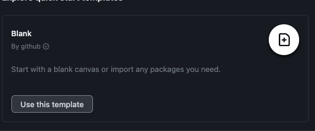
Clicking on “Use this template” launches a codespace in a separate tab within your browser.
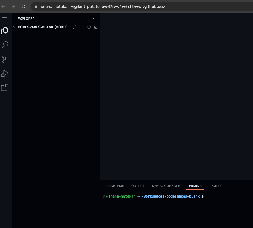
My new codespace is called “vigilant potato” as you can see from the URL in the screenshot above. Your codespace will get its own unique, and maybe cute, name.
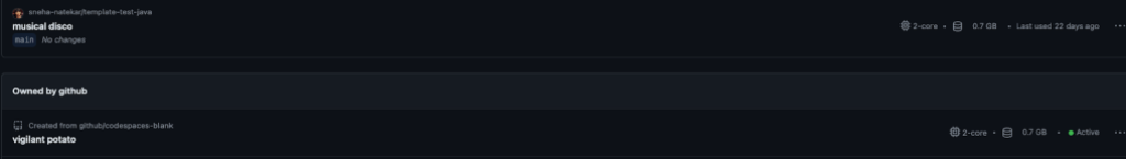
If you get distracted by something else, and need to come back to your codespace, you can access it from github.com/codespaces by looking for the “vigilant potato” among the list of codespaces—you might need to scroll down to find it if you have other codespaces.
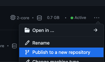
Click on the three horizontal dots at the end of the row and select “Publish to a new repository.” This flow seamlessly lets you create a new repository and preserves your development environment and any code you might have added that belongs to your project.
Once your repository is created, you’ll be able to see it in your GitHub Settings > your repositories. Or, if you’d like to connect to an existing repository, you can do so through the terminal.
Step 2: Configuring your environment: devcontainer.json/Dockerfile
There are two ways to customize your environment in a template. The two ways: using either a devcontainer.json file or a Dockerfile. The devcontainer.json file focuses on configuring the development environment within Visual Studio Code, while a Dockerfile allows you to create a custom Docker image that forms the basis of the entire development environment. Both files are essential for defining and customizing the development environment to meet the specific requirements of your project.
For my Android development environment, I have to create a Dockerfile. To harness this power, I simply navigate to the root of my repository and create a new file called Dockerfile. You can define the base image, specify environment variables, copy files and directories, install dependencies, execute commands, expose ports, define the working directory, run services, and set the entrypoint or command. These instructions allow you to tailor the Docker image to include the necessary tools, configurations, and dependencies required for your project.
Watch the magic unfold as a tailored, fully-configured development environment materializes in the cloud. In an instant, you’ll be immersed in a seamless coding experience, equipped with all the necessary tools. Say goodbye to setup hassles and dive straight into your code. With a customized codespace template, you’ll have a portable development sanctuary that follows you everywhere. For my Android repository, I very easily followed these steps and a brand new codespace built from the blank template opened for my repository in a separate browser tab.
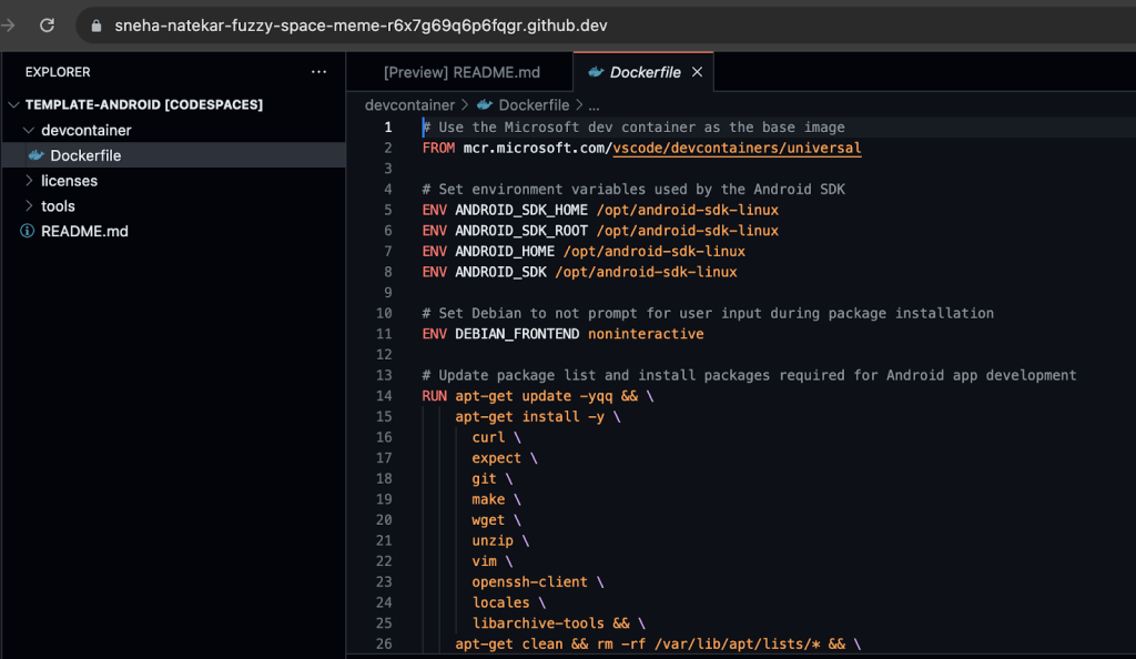
Here are a few snippets from my Android Dockerfile to demonstrate its power.
Automating Android SDK installation
# Update package list and install packages required for Android app development
RUN apt-get update -yqq && \
apt-get install -y \
curl \
expect \
git \
make \
wget \
unzip \
vim \
openssh-client \
locales \
libarchive-tools && \
apt-get clean && rm -rf /var/lib/apt/lists/* && \
localedef -i en_US -c -f UTF-8 -A /usr/share/locale/locale.alias en_US.UTF-8
In this example, I am using regular shell commands to install the Android SDK.
Setting environment variables
# Set environment variables used by the Android SDK
ENV ANDROID_SDK_HOME /opt/android-sdk-linux
ENV ANDROID_SDK_ROOT /opt/android-sdk-linux
ENV ANDROID_HOME /opt/android-sdk-linux
ENV ANDROID_SDK /opt/android-sdk-linux
This snippet showcases how the Dockerfile lets you set environment variables that are necessary for development.
This remarkable file guarantees a breeze for anyone cloning my repository, effortlessly setting up a standardized development environment. Say goodbye to manual setup hassles and welcome a seamless and efficient collaborative experience.
Conclusion
By embracing these steps, I’ve discovered that the entire process of creating and using GitHub Codespaces templates can be incredibly easy, enjoyable, and efficient. Leveraging the power of templates and devcontainer.json files means I never have to start from scratch again. What used to be a painstaking, day plus process of downloading and installing all of the Android SDK and Java components, setting the environment variables, getting the libraries, and maintaining their updates is no more through using my pre-configured Android template. I have created additional templates for work that are Java and Python development environments.
Remember, with great coding comes great responsibility,and a lot fewer debugging sessions! Happy coding, and may the bugs be ever in your favor!
If you’re also an Android developer, try out my template or explore the other templates GitHub offers and customize your own.
The post Unleashing GitHub Codespaces templates to ignite your development appeared first on The GitHub Blog.
[$] A more dynamic software I/O TLB
Post Syndicated from corbet original https://lwn.net/Articles/940973/
The kernel’s software I/O translation lookaside buffer (“swiotlb”) is an
obscure corner of the DMA-support layer. The swiotlb was initially
introduced to enable DMA for devices with special challenges, and one might
have expected it to fade away as newer peripherals came along. Instead,
though, the swiotlb has turned out to be useful in places outside of its
original use cases. This
patch set from Petr Tesarik now aims to update the swiotlb with an eye
toward its continuing use indefinitely into the future.
Rust 1.72.0 released
Post Syndicated from corbet original https://lwn.net/Articles/942656/
Version
1.72.0 of the Rust compiler has been released. Changes include
improved diagnostics and the removal of a limit on const evaluation:
To prevent user-provided const evaluation from getting into a
compile-time infinite loop or otherwise taking unbounded time at
compile time, Rust previously limited the maximum number of
statements run as part of any given constant evaluation. However,
especially creative Rust code could hit these limits and produce a
compiler error. Worse, whether code hit the limit could vary wildly
based on libraries invoked by the user; if a library you invoked
split a statement into two within one of its functions, your code
could then fail to compile.Now, you can do an unlimited amount of const evaluation at compile
time.
Security updates for Thursday
Post Syndicated from jake original https://lwn.net/Articles/942654/
Security updates have been issued by Debian (w3m), Fedora (libqb), Mageia (docker-containerd, kernel, kernel-linus, microcode, php, redis, and samba), Oracle (kernel, kernel-container, and openssh), Scientific Linux (subscription-manager), SUSE (ca-certificates-mozilla, erlang, gawk, gstreamer-plugins-base, indent, java-1_8_0-ibm, kernel, kernel-firmware, krb5, libcares2, nodejs14, nodejs16, openssl-1_1, openssl-3, poppler, postfix, redis, webkit2gtk3, and xen), and Ubuntu (php8.1).
Приключи проектът, стимулиращ гражданска активност сред украинските бежанци в Бургаска област
Post Syndicated from Биволъ original https://bivol.bg/proekt-ukrainci.html
четвъртък 24 август 2023

С поредица от информационни дни приключи проектът „Виртуален хайд парк „Гласът на младите” – стимулиране на гражданска активност сред украински младежи – бежанци в България”. Проектът бе изпълнен от Сдружение…
Star your favorite websites in the dashboard
Post Syndicated from Emily Flannery original http://blog.cloudflare.com/star-your-favorite-websites-in-the-dashboard/


We’re excited to introduce starring, a new dashboard feature built to speed up your workflow. You can now “star” up to 10 of the websites and applications you have on Cloudflare for quicker access.
Star your websites or applications for more efficiency
We have heard from many of our users, particularly ones with tens to hundreds of websites and applications running on Cloudflare, about the need to “favorite” the ones they monitor or configure most often. For example, domains or subdomains that our users designate for development or staging may be accessed in the Cloudflare dashboard daily during a build, migration or a first-time configuration, but then rarely touched for months at a time; yet every time logging in, these users have had to go through multiple steps—searching and paging through results—to navigate to where they need to go. These users seek a more efficient workflow to get to their destination faster. Now, by starring your websites or applications, you can have easier access.
How to get started
Star a website or application
Today, you can star up to 10 items per account. Simply star a website or application you have added to Cloudflare from its Overview page. Once you have starred at least one item, you will then see these marked as “starred” in most places across the dashboard. Just look for the yellow star icon. You can always remove from starred by toggling the button.
Filter by starred
By starring a website or application, you can then filter your lists down to display starred items only. To do so, simply select the “starred” filter from the Home page or the site switcher from the sidebar navigation.
Try it out for yourself—log into your account to get started today.
What’s next?
We're very excited to offer this new functionality for better organization of your Cloudflare experience, and about the many possibilities to mature this feature. After trying it out, give us a shout in the Cloudflare Community to let us know what improvements you’d like to see come next.
Why Your AWS Cloud Container Needs Client-Side Security
Post Syndicated from Rapid7 original https://blog.rapid7.com/2023/08/24/why-your-aws-cloud-container-needs-client-side-security/

With increasingly complicated network infrastructure and organizations needing to deploy applications across various environments, cloud containers are necessary for companies to stay agile and innovative. Containers are packages of software that hold all of the necessary components for an app to run in any environment. One of the biggest benefits of cloud containers? They virtualize an operating system, enabling users to access from private data centers, public clouds, and even laptops.
According to recent research by Faction, 92% of organizations have a multi-cloud strategy in place or are in the process of adopting one. In addition to the ubiquity of cloud computing, there are a variety of cloud container providers, including Google Cloud Platform (GCP), Amazon Web Services (AWS), and Microsoft Azure. Nearly 80% of all containers on the cloud, however, run on AWS, which is known for its security, reliability, and scalability.
When it comes to cloud container security, AWS works on a shared responsibility model. This means that security and compliance is shared between AWS and the client. AWS protects the infrastructure running the services offered in the cloud — the hardware, software, networking, and facilities.
Unfortunately, many AWS users stop here. They believe that the security provided by AWS is sufficient to protect their cloud containers. While it is true that the level of customer responsibility for security differs depending on the AWS product, each product does require the customer to assume some level of security responsibility.
To avoid this mistake, let’s examine why your AWS cloud container needs additional client-side security and how Rapid7 can help.
Top reasons why your AWS container needs client-side security
Visibility and monitoring
Some of the same qualities that make containers ideal for agility and innovation also creates difficulty in visibility and monitoring. Cloud containers are ephemeral, which means they’re easy to establish and destroy. This is convenient for quickly moving workloads and applications, but it also makes it difficult to track changes. Many AWS containers share memory and CPU resources with a variety of hosts (physical and cloud) in your ecosystem. Consequently, monitoring resource consumption and assessing container performance and application health can be difficult — after all, how can you know how much memory is being utilized by the container or the physical host?
Traditional monitoring tools and solutions also fail to collect the necessary metrics or provide the crucial insights needed for monitoring and troubleshooting container health and performance. While AWS offers protection for the cloud container structure, visualizing and monitoring what happens within the container is the responsibility of your organization.
Alert contextualization and remediation
As your company grows and you scale your cloud infrastructure, your DevOps teams will continue to create containers. For example, Google runs everything in containers and launches an epic amount of containers (several billion per week!) to keep up with their developer and client needs. While you might not be launching quite as many containers, it’s still easy to lose track of them all. Organizations utilize alerts to keep track of container performance and health to resolve problems quickly. While alerting policies differ, most companies use metric- or log-based alerting.
It can be overwhelming to manage and remediate all of your organization’s container alerts. Not only do these alerts need to be routed to the proper developer or resource owner, but they also need to be remediated quickly to ensure the security and continued good performance of the container.
Cybersecurity standards
While AWS provides security for your foundational services in containerized applications — computing, storage, databases, and networking — it’s your responsibility to develop sufficient security protocols to protect your data, applications, operating system, and firewall. In the same way that your organization follows external cybersecurity standards for security and compliance across the rest of your digital ecosystem, it’s best to align your client-side AWS container security with a well-known industry framework.
Adopting a standardized cybersecurity framework will work in concert with AWS’s security measures by providing guidelines and best practices — preventing your organization from a haphazard security application that creates coverage gaps.
How Rapid7 can help with AWS container security
Now that you know why your organization needs client-side security, here’s how Rapid7 can help.
- Visibility and monitoring: Rapid7’s InsightCloudSec continuously scans your cloud’s infrastructure, orchestration platforms, and workloads to provide a real-time assessment of health, performance, and risk. With the ability to scan containers in less than 60 seconds, your team will be able to quickly and accurately track changes in your containers and view the data in a single, convenient platform, perfect for collaborating across teams and quickly remediating issues.
- Alert contextualization and remediation: Client-side security measures are key to processing and remediating system alerts in your AWS containers, but it can’t be accomplished manually. Automation is key for alert contextualization and remediation. InsightCloudSec integrates with AWS services like Amazon GuardDuty to analyze logs for malicious activity. The tool also integrates with your larger enterprise security systems to automate the remediation of critical risks in real time — often within 60 seconds.
- Cybersecurity standards: While aligning your cloud containers with an industry-standard cybersecurity framework is a necessity, it’s often a struggle. Maintaining security and compliance requirements requires specialized knowledge and expertise. With record staff shortages, this often falls by the wayside. InsightCloudSec automates cloud compliance for well-known industry standards like the National Institute of Standards and Technology’s (NIST) Cybersecurity Framework (CSF) with out-of-the-box policies that map back to specific NIST directives.
Secure your container (and it’s contents)
AWS’s shared responsibility model of security helps relieve operational burdens for organizations operating cloud containers. AWS clients don’t have to worry about the infrastructure security of their cloud containers. The contents in the cloud containers, however, are the owner’s responsibility and require additional security considerations.
Client-side security is necessary for proper monitoring and visibility, reduction in alert fatigue and real-time troubleshooting, and the application of external cybersecurity frameworks. The right tools, like Rapid7’s InsightCloudSec, can provide crucial support in each of these areas and beyond, filling crucial expertise and staffing gaps on your team and empowering your organization to confidently (and securely) utilize cloud containers.
Want to learn more about AWS container security? Download Fortify Your Containerized Apps With Rapid7 on AWS.
Parmesan Anti-Forgery Protection
Post Syndicated from Bruce Schneier original https://www.schneier.com/blog/archives/2023/08/parmesan-anti-forgery-protection.html
The Guardian is reporting about microchips in wheels of Parmesan cheese as an anti-forgery measure.
[$] LWN.net Weekly Edition for August 24, 2023
Post Syndicated from corbet original https://lwn.net/Articles/941867/
The LWN.net Weekly Edition for August 24, 2023 is available.
Megan Rapinoe Answers the Critics
Post Syndicated from The Atlantic original https://www.youtube.com/watch?v=SiUxXX_RR_U