Post Syndicated from LGR original https://www.youtube.com/watch?v=-zezLB3sVW0
Security updates for Friday
Post Syndicated from original https://lwn.net/Articles/938233/
Security updates have been issued by Debian (lemonldap-ng and php-dompdf), Red Hat (.NET 6.0, .NET 7.0, firefox, and thunderbird), Scientific Linux (firefox and thunderbird), SUSE (ghostscript, installation-images, kernel, php7, python, and python-Django), and Ubuntu (linux-azure, linux-gcp, linux-ibm, linux-oracle, mozjs102, postgresql-9.5, and tiff).
Вече няма нито „добри“, нито „лоши“
Post Syndicated from Емилия Милчева original https://www.toest.bg/veche-nyama-nito-dobri-nito-loshi/

Големите управляващи коалиции в България си намират външнополитически основания. Членството в Европейския съюз обоснова правителството на тройната коалиция – БСП, ДПС и НДСВ. Заради Шенген, еврозоната и войната в Украйна ПП–ДБ получава подкрепа от ГЕРБ–СДС, а те пък очакват да им дойде ротацията след по-малко от 9 месеца и да управляват със свой кабинет.
Така Европа и западните съюзници получават предвидим партньор в лицето на България, а българското общество – халтава сглобка, чиито съставни части се борят със стръв за места в регулаторите и институциите с няколкогодишни мандати. Към сглобката бе прилепено и ДПС – чрез формулата за „конституционно мнозинство“ и със съдействието на ГЕРБ. Ето че „добрите“ и „лошите“ вече са едно управление – нито „добро“, нито „лошо“, нито добролошо, но със сигурност трудно за преглъщане от избирателите на ПП–ДБ.
„Пропагандният приапизъм“ (израз, с който коментатор в социалните мрежи определи пилона в Рожен) вече отстъпи място на прагматизма, предпочитан от политиците в не-изборни времена. Особено при подялбата на постове, от чиито решения зависят много бизнеси и разпределяне на милиарди.
Подбор в тесен (троен) кръг
Вече няма съмнение, че коалиционно споразумение няма да има. Заглъхнаха всякакви сигнали и от ПП–ДБ, и от ГЕРБ–СДС да има някакви публично известни правила, по които ще стават назначенията, а през това време ДПС тихо консумира, без да вдига шум. Modus operandi e намерен, след като се разпределят позиции в регулатори и институции. Изчезна и онази първоначална свенливост на обединените в не-коалиция политически сили.
В Народното събрание става раздаването на председателските места в постоянните комисии, в резултат на което ГЕРБ–СДС взе 15, ДПС – пет, а ПП–ДБ – три. Гладкото протичане на гласуването е доказателство, че всичко е било предварително съгласувано. Председател на Бюджетната комисия стана Йордан Цонев (ДПС), един от най-големите критици на политиката на финансовия министър Асен Василев, а Делян Пеевски бе включен в Правната. Външната комисия оглави лидерът на ГЕРБ Бойко Борисов – огледално на позицията външен министър, която заема в правителството представителката на ГЕРБ Мария Габриел. Така Борисов, чието чисто съдебно минало не е заплашено от „Барселонагейт“, Иван Гешев или нещо друго, е видим в бяло за европейските и евроатлантическите партньори.
Синхрон като с комисиите се получава и с ръководството на БНБ – гуверньор за втори 6-годишен мандат остава Димитър Радев, кандидат на ГЕРБ–СДС. Въпреки че двамата подуправители не са официално обявени (формално Радев трябва да внесе кандидатурите им в парламента, след като бъде избран), най-вероятните ще са Андрей Гюров от ПП, неуспял кандидат за управител на БНБ в 47-мия парламент, и Петър Чобанов от ДПС. Това ще е екипът, който ще носи отговорността за присъединяването на България към еврото, ако се въведе от 1 януари 2025 г. – заедно с третия подуправител Радослав Миленков от сферата на влияние на ГЕРБ & ДПС, чийто мандат изтича същата година.
Трудността да се споразумеят за управител на Здравната каса, след като не бе харесана кандидатката на ГЕРБ Иванка Динева, предизвика промяна на закона – подуправителят да изпълнява безсрочно длъжността до избирането на титуляр. Едва ли ГЕРБ и ДПС ще позволят някой извън тяхната сфера на влияние да разпределя бюджета на НЗОК – 7,27 млрд. лв. за тази година, с 910 млн. повече от предходната. Лъвският пай от тази сума винаги е за болниците – почти 50%, макар за 2023 г. да е 45%. Средно за ЕС този процент е 30%, тъй като в развитите европейски държави ударението е върху превенцията.
Сметната палата, чиято работа е да следи целесъобразно и ефективно ли се харчат публичните средства, също ще получи гербер за шеф. Партията на Бойко Борисов издигна лоялен партиец – Димитър Главчев, за председател на институцията, от която зависят контролът и (не)прикриването на корупцията. ПП–ДБ не възразяват.
До началото на парламентарната ваканция през август остават две седмици и управляващото мнозинство едва ли ще премине и към другите регулатори, които очакват обновяване – КЕВР, КФН, КЗК и др. Още повече че към момента не са назначени и всички областни управители. Първите шест от общо 28 станаха известни тази седмица и те са на София-град, Пловдив, Ловеч, Плевен, Добрич и Силистра. До избора на следващите по местата си остават избраните от служебния кабинет на президента.
Съдебната реформа – възпряна от реформаторите
Крехкият позитивизъм покрай съставянето на правителството бързо се разсея заради правените на тъмно кадрови договорки. И не само. 45 дни след като окончателно беше приет механизмът за контрол на главния прокурор, очакван 12 години, конституционното мнозинство – ПП–ДБ, ГЕРБ–СДС и ДПС, реши да поправи промените в Наказателно-процесуалния кодекс и Закона за съдебната власт, които го въвеждат. Без публични обяснения и ясна обосновка. С подписите на Десислава Атанасова (ГЕРБ), Кирил Петков (ПП–ДБ), Атанас Атанасов (ПП–ДБ), Надежда Йорданова (ПП–ДБ) и Хамид Хамид (ДПС) беше предложено изборът на разследващ главния прокурор да става по нова, несъздадена още система, различна от Единната информационна система на съдилищата (EИСС).
ЕИСС е платформа за управление на съдебните дела, създадена от държавната фирма „Информационно обслужване“, която обхваща всички съдилища, и чрез нея се генерира случайното разпределение на делата. Процесът е обвеян със съмнения за неслучайност при някои дела. Както отбелязаха юристи, излиза, че за разследващ главния прокурор се прави специална система, но не се променя ЕИСС за останалите дела. Заместник-председателката на Върховния касационен съд Лада Паунова отбеляза по повода, че това ще срине доверието в настоящата система.
Законопроектът се появи веднага след като на случаен принцип във ВКС от 22-ма съдии, съгласили се да разследват престъпления на главния прокурор, беше избрана съдия Даниела Талева за ad hoc прокурор. Тя трябваше да разследва сигнали, сред които и за имотното състояние, срещу изпълняващия функцията главен прокурор Борислав Сарафов. Прокурорската колегия на ВСС – същата, която бързо-бързо избра Сарафов за и.ф., обаче отказа да я назначи.
Намериха се и мотиви, и те са същите, с които прокурорската колегия спря процедурата за избор на нов главен прокурор – делото пред Конституционния съд, образувано по искане на бившия главен прокурор Иван Гешев. Той оспорва законовите промени, които въвеждат механизма за разследване на обвинител №1. Със същия аргумент конституционното мнозинство – ГЕРБ–СДС, ПП–ДБ и ДПС, призова в безпрецедентна декларация ВСС да прекрати процедурата за избор на нов главен прокурор, добавяйки и предвижданите промени в Конституцията (които ще станат неясно кога).
Резултатът от всички тези действия е, че Сарафов – дясната ръка на Гешев, обърнала се срещу него, може да си отдъхне, и то задълго. Нищо не го застрашава. Няма законови санкции за прокурорската колегия, ако блокира назначаването на разследващ главния прокурор – законодателите от ГЕРБ, ПП–ДБ и ДПС не ги разписаха. А срок, в който да стане, не е посочен. Така че няма особена сила призивът на правосъдния министър Атанас Славов прокурорската колегия на ВСС да продължи започналата процедура по механизма за разследване на главния прокурор и неговите заместници, като назначи съдия Даниела Талева за прокурор, работещ по сигналите срещу Сарафов.
Не е ясно и колко бързо ще се направи нова система за избор. Когато един ден стане готова, пак ще има избор на прокурор ad hoc, но няма да е Талева.
Наред с промяната в механизма за разследващ главния прокурор, от три на шест месеца беше удължен срокът, в който да бъде избран нов Висш съдебен съвет, който пък трябва да избере нов главен прокурор. Мандатът на настоящия ВСС е изтекъл миналата година и вместо да избере нов, както повелява законът, парламентарното мнозинство определи през май т.г. един срок, който се оказа, че няма да изпълни – и повторно го удължи.
Всички тези законодателни промени минаха през Правната комисия скорострелно, както и предишните. Също така спешно бяха внесени в пленарната зала, бързичко и без шум приети, а срокът между първо и второ четене – съкратен на три дни.
Случващото се хвърля сянка върху реформаторите, след като фундаментът на тяхната реформа е на поправителен малко повече от месец след приемането му, което произведе шумни аплаузи. Заради приемането на механизма 49-тият парламент избра най-напред председател на Правната комисия – единствената с такъв в продължение на няколко седмици.
Е, ако не друго, конституционното мнозинство работи – макар и не по Конституцията.
Quickly see differences between Zone Versions with Version Comparisons
Post Syndicated from Garrett Galow original http://blog.cloudflare.com/quickly-see-differences-between-zone-versions-with-version-comparisons/


On the week of July 10, 2023, we launched a new capability for Zone Versioning – Version Comparisons. With Version Comparisons, you can quickly get a side by side glance of what changes were made between two versions. This makes it easier to evaluate that a new version of your zone’s configuration is correct before deploying to production.
A quick recap about Zone Versioning
Zone Versioning was launched at the start of 2023 to all Cloudflare Enterprise customers and allows you to create and manage independent versions of your zone configuration. This enables you to safely configure a set of configuration changes and progressively roll out those changes together to predefined environments of traffic. Having the ability to carefully test changes in a test or staging environment before deploying them to production, can help catch configuration issues before they can have a large impact on your zone’s traffic. See the general availability announcement blog for a deeper dive on the overall capability.
Why we built Version Comparisons
Diff is a well known and often used tool by many software developers to quickly understand the difference between two files. While originally just a command line utility it is now ubiquitous across the software world. Most commonly used in code reviews, software developers use ‘diffs’ to ensure they can validate the set of changes they intend to make to a codebase and to allow others to easily review their code by focusing on what changed. One of the drawbacks of graphical user interfaces (GUIs) for managing configurations is since they aren’t ‘files’, tools like diff don’t work for them. This was true with Zone Versioning, as to try and understand what had changed between two versions you would need to manually inspect each version and the various sections of the dashboard across both versions. This is quite tedious and error-prone, so it can reduce the safety that versioning can provide.
With Version Comparisons, we are bringing the same capabilities of diff but without the need for using a command line to allow customers to compare two versions side by side. This makes the process of understanding which configurations of your zone changed between two versions easy, quick and painless. By pointing out which config has changed, you can have greater confidence that deploying a new version of your configuration will not create any surprises. Let’s now look at how to use Version Comparisons in the Cloudflare Dashboard.
Using Version Comparisons
After navigating to a zone that has Zone Versioning enabled, select ‘Version Management’ in the left-hand navigation. For help getting started with Zone Versioning, see our dev docs.
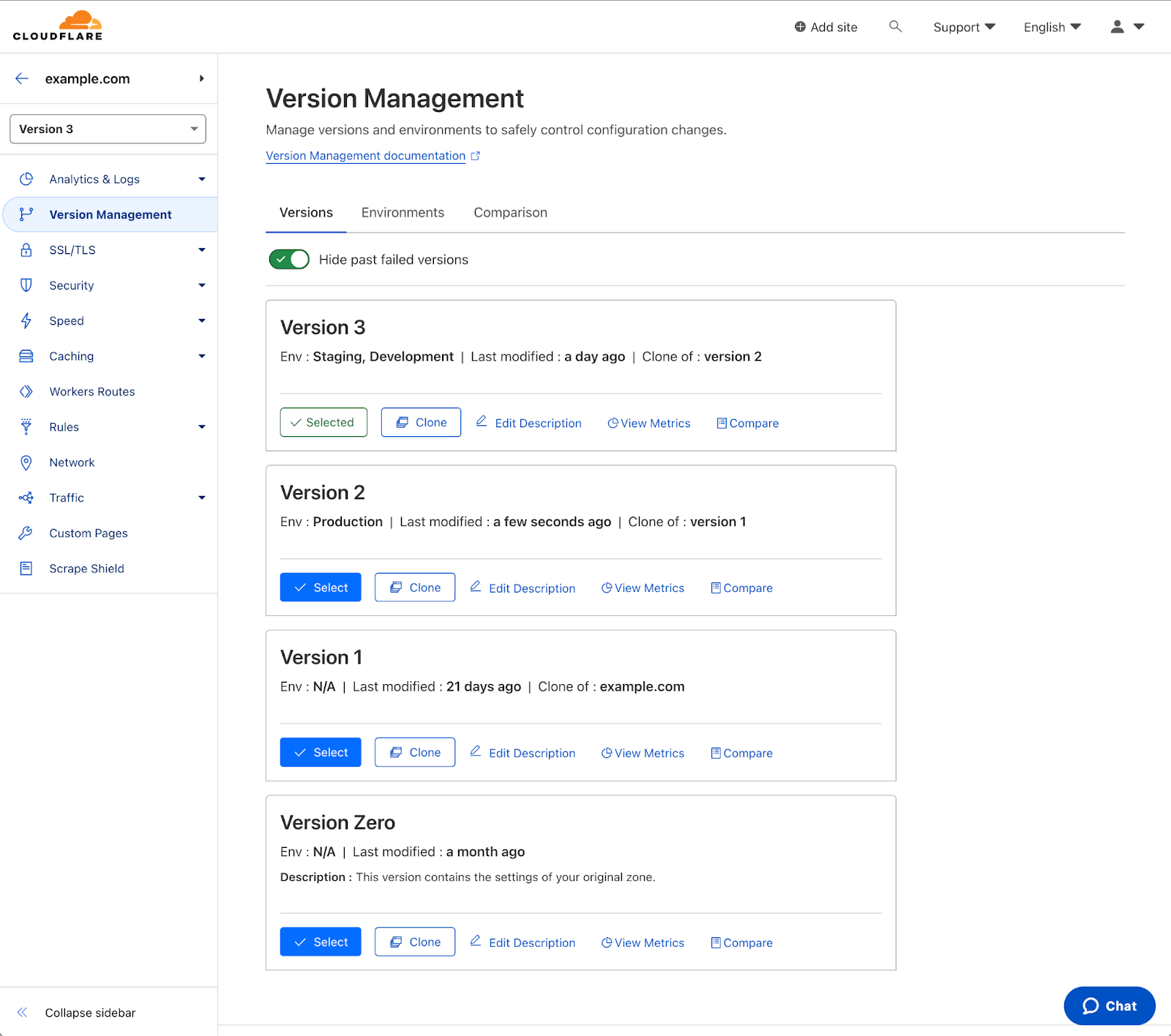
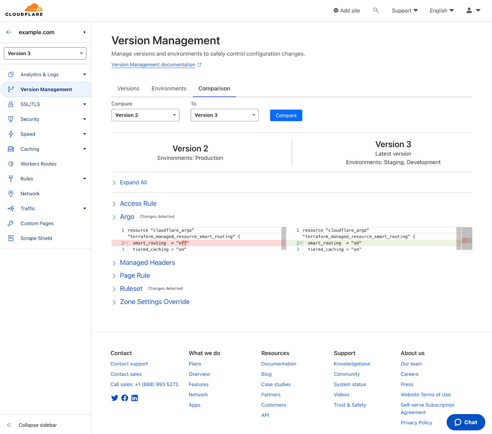
After selecting the ‘Version Management’ tab you will notice a third option – ‘Comparisons’. Selecting that will prompt you to select two versions to compare. Select the two version you want to compare and then select ‘Compare’
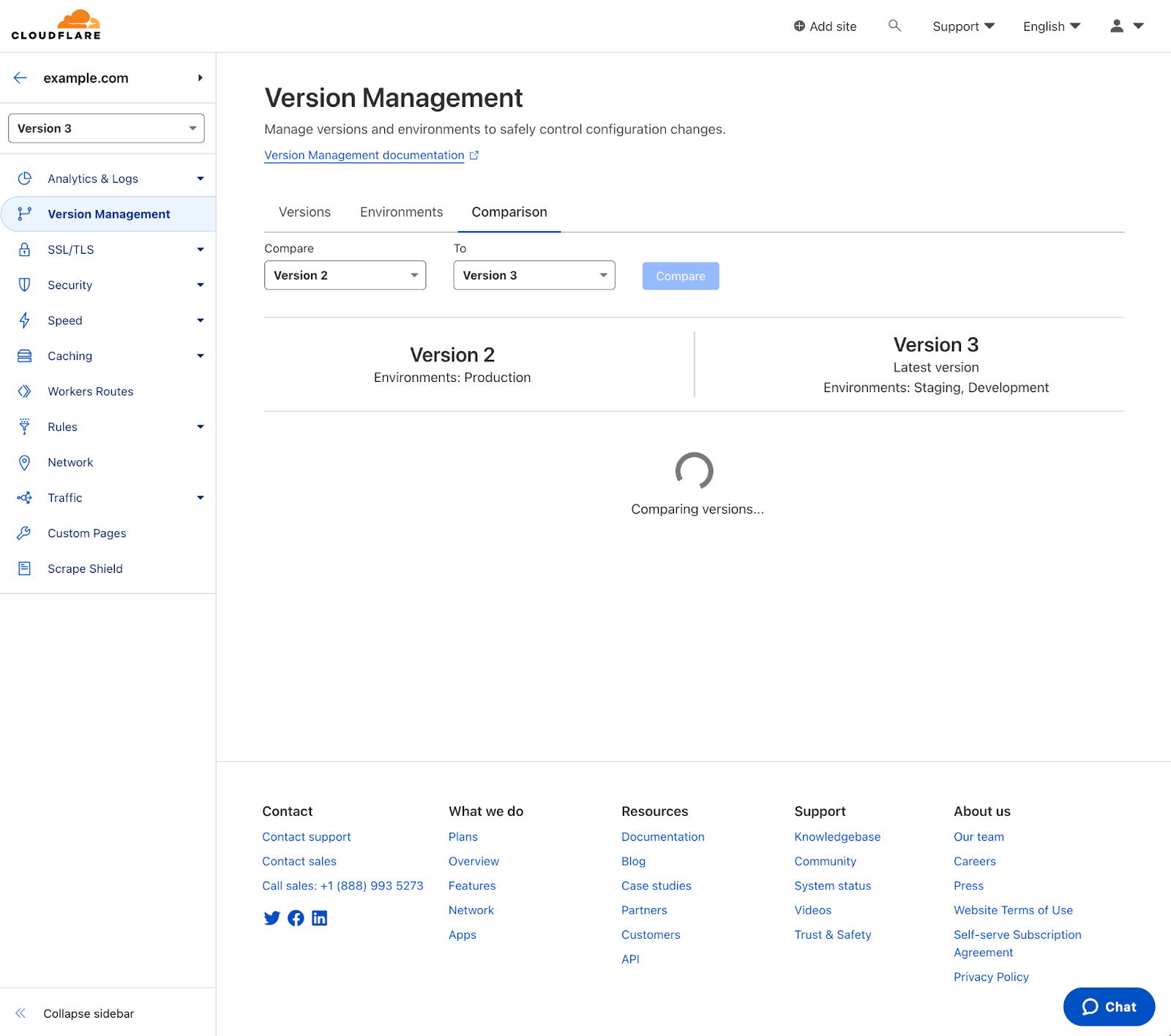
After a few seconds, the page will update automatically with a comparison on a per-product basis. The lower numbered version will always be presented on the left and the top will show you which environments the versions are assigned to so that you can ensure you are comparing the right versions. A common use case would be to compare the versions in staging and production to verify the changes before promoting the staging version to production.
Any products with changes will have ‘changes detected’ noted next to them. Selecting one will open up the diff of that product across both versions.

Changes will be highlighted for new additions and removals for that service. Based on the comparison, you can then decide if more changes are necessary or if that new version is ready to be rolled out.
Try out Version Comparisons today
Versions comparisons are available to all customers using Zone Versioning! If you are a Cloudflare Enterprise customer, to get started using Zone Versioning and Version Comparisons, check out our dev docs.
When Whales Attack
Post Syndicated from The History Guy: History Deserves to Be Remembered original https://www.youtube.com/watch?v=iT4kRth_2-c
Научни новини: ГМО и глобално затопляне
Post Syndicated from Михаил Ангелов original https://www.toest.bg/nauchni-novini-gmo-i-globalno-zatoplyane/
Промяна на ГМО хоризонта

През последните 10–15 години възможностите за редактиране на генома на културните растения се разшириха значително и учените вече имат по-прецизни и по-лесни за употреба инструменти, като ZFNs, TALENs и най-новия CRISPR/Cas9. Тези методи са основата на т.нар. нови геномни техники (НГТ) и бяха в своеобразна сива зона в Европа, защото нямаше пълна яснота дали растенията, получени с тяхна помощ, попадат в категорията на „класическите“ ГМО.
С решение на Съда на Европейския съюз от средата на 2018 г. бе установено, че към новите геномни техники ще се прилага съществуващото законодателство за ГМО. Въпреки че позицията на повечето учени, включително от Европейския орган за безопасност на храните (ЕОБХ), е, че те са по-безопасни от старите методи за генетични манипулации, това решение донякъде не беше изненада поради традиционно консервативния подход на ЕС в тази област.
Но ситуацията може да се промени – след проучване на НГТ Европейската комисия предлага преразглеждане на сегашните регулации и облекчаването им за някои растения. В предложението се въвеждат две категории, в които ще попадат растенията в зависимост от вида, броя и размера на генетичните модификации на генома.
Категория 1 ще покрива растения с промени, които може да се срещнат в природата или да се постигнат с традиционните техники за селекция. Това ограничава потенциалните промени до насочена мутагенеза (промяна на конкретни участъци от ДНК, в повечето случаи с цел инактивиране на гени) и цисгенеза (прехвърляне на генетичен материал от два близкородствени организма).
Преди пускането им на пазара те ще минават през процедура на верификация, но тя ще бъде значително облекчена и ускорена, а след това растенията ще бъдат третирани като получени от конвенционална селекция. Все пак при съществени промени на състава и хранителните им качества ще попадат под регулациите за нови храни в ЕС и ще минават за одобрение през ЕОБХ.
Може би най-спорната част е НГТ произходът да бъде означен само на семената, използвани от земеделците, а всички продукти, които стигат до крайния потребител, да бъдат разглеждани като конвенционални. Все пак тези растения няма да могат да се сертифицират като „органични“, което донякъде ще ги различава. Най-вероятно обект на възражения ще бъде и условието, че отделните страни членки няма да могат да забранят полските опити и отглеждането на тези растения.
В предложението се говори и за проследяемост, но е интересно как ще бъде реализиран този процес, защото за разлика от по-старите методи за намеса в генома, промяната с помощта на НГТ е недоловима.
За останалите растения (категория 2) ще продължат да важат сегашните регулации за ГМО. Тук ще се включват трансгенетичните растения (с вмъкнато ДНК от различни организми), растенията с екстензивни редакции и някои други изключения.
Предложението за промяна идва в динамичен момент в глобален мащаб. От особена важност е въвеждането на нови сортове, които ще са ключови за изхранването ни на фона на настъпващите климатични промени. Друг значим фактор е опасността от изоставане в сферата на генетичните редакции както в научен, така и икономически аспект. Регулациите за този тип генетични редакции са значително по-облекчени в САЩ, Индия, Китай, Великобритания и редица други държави, което прави развитието на иновации в сферата по-лесно и по-изгодно. В документа се споменават също пандемията от COVID-19 и войната в Украйна, разкрили външните зависимости на Европа.
Очаквано, научните среди и биотехнологичните компании приемат новината добре. Според оценката на ЕК промяната в регулациите би спестила милиони евро годишно и така разработването на нови сортове ще стане по-достъпно, а административните разходи ще намалеят. В подкрепа на предложението за облекчаване на регулациите е и организацията EU-SAGE („Устойчиво земеделие чрез генетични редакции в Европа“), в която членуват учени от над 150 европейски института, три от които български.
Редица организации се противопоставят със становището, че промените ще влошат качеството на храната. Има също опасения, че селекцията на нови видове ще бъде консолидирана в ограничен брой биотехнологични гиганти, което ще доведе до по-високи цени на семената, и ще бъде ограничена свободата на фермерите. Събрани са и над 400 000 подписа в петиция, която според организаторите ѝ ще покаже преобладаващото негативно мнение на жителите на ЕС.
В процеса на обсъждане най-вероятно ще настъпят промени в детайлите, но след като бъдат приети от ЕК, новите правила ще трябва да бъдат гласувани и в Европейския парламент, където също се очаква да има разгорещени дебати. Важното е, че дискусията е започнала и има възможност да се стигне до решение, което да е в крак с промените – както климатични, така и научни.
Планетата се затопля
За съжаление, глобалните климатични промени не чакат обсъжданията. В няколко поредни юлски дни бяха счупени температурните рекорди и се очаква 2023-та да е най-горещата година от последните над 200, в които се правят точни измервания. Ако се включат и палеоклиматичните данни, този период може да достигне 120 000 години.
Справка в поддържания от Университета на Мейн Climate Reanalyzer показва, че средната глобална температура е достигнала 17,23°C на 6 юли. Един от рекордите е потвърден и от Европейската услуга за проследяване на климатичните промени, в която се използват данни от спътниците „Коперник“. Учените отбелязват, че това може да е вследствие на времето в Южното полукълбо и потока от необичайно горещ въздух над части от Антарктида, но промените са отчетени и в много други точки на света. В алжирския град Адрар температурата не е паднала под 39,6°C дори и през нощта. А след два смъртни случая в Пекин поради високите температури, в редица градове в Китай бяха отворени бомбоубежищата и бе забранена работата на открито.
Една от основните причини за високите температури е Ел Ниньо – топлата фаза на Южното колебание, чийто интензитет този път е особено висок. Това донякъде беше очаквано заради нехарактерно голямата продължителност на предхождащата студена фаза (Ла Ниня). Тъй като пикът на топлата фаза обикновено е между ноември и януари, се очаква ефектът му да се засили през идните месеци, като не е изключено да продължи и по-дълго от обичайното, както стана и при предхождащата Ла Ниня.
За интензитета на Ел Ниньо е ключова температурата на океанската вода, защото при него само се прехвърля топлина от океана към атмосферата. А океанът се затопля – според данни на Европейската услуга за проследяване на климатичните промени температурата на океана през юни е с 0,91°C над средната за периода 1979–2023 г. и с около 0,5°C по-висока от предишния юнски рекорд, отчетен през 2010 г. Особено топли са североизточните части на Атлантика, където температурите са достигнали 1,36°C над средното.
Поради затоплянето на горните слоеве на океана, изкачването на студената вода от дълбочините се забавя и се образува своеобразна възглавница от топла вода. Така топлината, която океанът е поел през трите години на Ла Ниня, сега се освобождава. Този фронт предизвиква и повече гръмотевични бури, което допълнително затопля атмосферата.
Високите температури са само едно от следствията на глобалните климатични промени. Водният цикъл на планетата също се влияе и променя по опасен начин. Испания е засегната от суша, която може да се окаже рекордна за последния век с 36 последователни месеца с валежи по-ниски от средната стойност. Съчетано с високите температури, това вещае катастрофална година за земеделците. Проблеми има и с питейната вода. Нивото на язовира Sau Reservoir в Каталуния е едва на 7% от капацитета му през април. Това е наложило и премахването на рибата от него, тъй като водата вече е била негодна за живот. На този фон наводнения в Индия засегнаха над половин милион души, като проливните дъждове са довели до преливането на река Беки и евакуацията на около 14 000 души. Наводнения с жертви имаше и в Япония и Турция.
В Канада бушуват опустошителни горски пожари, димът от които покри северните части на САЩ. Изгорели са над 9 млн. хектара – два пъти повече от обработваемите площи в България, а властите предупреждават, че тази година опасният сезон ще е по-продължителен. Мащабите са безпрецедентни и освен че имат унищожителни последици, пожарите ще влошат дългосрочно климата – въглеродните емисии са много по-високи от предходни години, а кумулативната топлина, отделена от огъня до момента, е почти два пъти повече, отколкото за цялата рекордна 2022 година. Най-вероятно ранното начало на сезона на пожарите се дължи на нехарактерните и дълги суши, комбинирани с необичайно високи температури. В началото на юли в северните части на провинция Квебек температурата е достигнала 34°C.
Промените са пагубни за всички обитатели на планетата. Затоплянето на океана, особено когато е рязко, както по време на Ел Ниньо, влияе зле и на обитателите му, и на птиците, които се хранят с тях. Ефектът от това не е незабавен, а може да се наблюдава след един до шест месеца според изследване на американски учени. Обобщени са данни от четири проекта за обследване на плажове, в които обучени доброволци броят мъртвите птици в конкретен участък.
Причините за смъртта на птиците са разнообразни, но повечето са свързани с променящите се екосистеми. Най-честата причина е промяна във видовия състав и размера на популациите в местата, в които те се хранят, водещо до гладна смърт. С промяната на самия океан е очаквано да настъпят промени и в организмите, които го обитават. Според авторите на статията мащабът на тези промени е голям и може да става въпрос за над милион загинали птици в периода 2014–2019 г. По-топлите води са добра среда за развитието на алги, които може да бъдат токсични за животните.
Топлинните вълни имат негативно влияние и върху насекомите. Ако температурата се повиши за три дни по време на възпроизвеждане, броят на потомството намалява двойно, а вероятността от успешно оплождане спада със 75%. Драстично спада и вероятността младите насекоми да оцелеят. Интересното е, че ако периодът на висока температура е малко преди или след периода на интимност, негативното му влияние е почти незначително. Резултатите от това изследване са важни, тъй като насекомите са основна част от хранителните вериги и над 89% от цъфтящите растения се опрашват от тях. В скорошна публикация е изказана хипотезата, че първите цъфтящи растения са били опрашвани от насекоми, а разпространението на полен с вятъра се е появило на по-късен етап.
Учените сигнализират за опасността от климатичните промени от десетилетия, но взетите мерки, изглежда, са твърде късни или недостатъчни. Протоколът от Киото и последващото Парижко споразумение дават рамка на световните правителства за намаляване на емисиите, но не е ясно дали те ще бъдат достатъчни. Планетата има известен буфер, най-вече в Световния океан, за поемане на допълнителна топлина, но той започва да се изчерпва и сме на ръба на събития, които ще бъдат каскадни и необратими. Въпреки че някои са скептични относно антропогенния характер на случващото се, то е факт и пред нас стоят множество проблеми, за които ще трябва да се намери решение.
Заглавно изображение: Язовир Sau Reservoir в Каталуния, заснет на 13 март 2023 г. Нивото на водоема е спаднало драстично оттогава. Снимка: European Union, Copernicus Sentinel-2 imagery
Buying Campaign Contributions as a Hack
Post Syndicated from Bruce Schneier original https://www.schneier.com/blog/archives/2023/07/buying-campaign-contributions-as-a-hack.html
The first Republican primary debate has a popularity threshold to determine who gets to appear: 40,000 individual contributors. Now there are a lot of conventional ways a candidate can get that many contributors. Doug Burgum came up with a novel idea: buy them:
A long-shot contender at the bottom of recent polls, Mr. Burgum is offering $20 gift cards to the first 50,000 people who donate at least $1 to his campaign. And one lucky donor, as his campaign advertised on Facebook, will have the chance to win a Yeti Tundra 45 cooler that typically costs more than $300—just for donating at least $1.
It’s actually a pretty good idea. He could have spent the money on direct mail, or personalized social media ads, or television ads. Instead, he buys gift cards at maybe two-thirds of face value (sellers calculate the advertising value, the additional revenue that comes from using them to buy something more expensive, and breakage when they’re not redeemed at all), and resells them. Plus, many contributors probably give him more than $1, and he got a lot of publicity over this.
Probably the cheapest way to get the contributors he needs. A clever hack.
EDITED TO ADD (7/16): These might be “straw donors” and illegal:
The campaign’s donations-for-cash strategy could raise potential legal concerns, said Paul Ryan, a campaign finance lawyer. Voters who make donations in exchange for gift cards, he said, might be considered straw donors because part or all of their donations are being reimbursed by the campaign.
“Federal law says ‘no person shall make a contribution in the name of another person,’” Mr. Ryan said. “Here, the candidate is making a contribution to himself in the name of all these individual donors.”
Richard L. Hasen, a law professor at the University of California, Los Angeles, who specializes in election law, said that typically, campaigns ask the Federal Election Commission when engaging in new forms of donations.
The Burgum campaign’s maneuver, he said, “certainly seems novel” and “raises concerns about whether it violates the prohibition on straw donations.”
Something for the courts to figure out, if this matter ever gets that far.
The End of Affirmative Action. For Real This Time.
Post Syndicated from The Atlantic original https://www.youtube.com/watch?v=ndX8a5Yy03w
Young people’s amazing experiments in space: Astro Pi Mission Space Lab 2022/23
Post Syndicated from Fergus Kirkpatrick original https://www.raspberrypi.org/blog/astro-pi-mission-space-lab-2022-23-results/
Celebrate another year of young people’s computer programs in space with us: today we and our collaborators at the European Space Agency can finally announce the winning and highly commended teams in this year’s Astro Pi Mission Space Lab.

Mission Space Lab: Young people’s experiments in space
In Mission Space Lab, teams of young people work together to create computer programs for scientific experiments to be carried out on the International Space Station. The programs they design and create run on the two Astro Pi computers: space-adapted Raspberry Pis with cameras and a range of sensors.

Teams’ programs were deployed on the ISS during May and ran for up to 3 hours, collecting data for their experiments. Once we’d sent the teams their data, they started analysing it in order to write their Phase 4 reports. To identify patterns and phenomena they were interested in, many teams chose to compare their data with other sources.

We were especially excited to see the results from the experiments this year, particularly given that the upgraded Astro Pi units with their High Quality Cameras were positioned in a new observation window (WORF) on the ISS. This allowed teams to capture high-resolution images with a much wider field of view.

What have Mission Space Lab teams investigated this year?
We feel very privileged to see the culmination of the team’s experiments in their final reports. So let’s share a few highlights from this year’s experiments:
Team Aretusa from Sicily explored the effects of climate change by cross-referencing the images they captured with the Astro Pis with historical images from Google Earth. They used Near Infrared photography to capture images, and NDVI (Normalised Difference Vegetation Index) image processing in their analysis. Below you can see that they have compared data of Saudi Arabia from 1987 to 2023, showing increasing levels of vegetation grown in attempts to restore degraded land.

Team Barrande from the Czech Republic trained AI models on images they gathered to identify topographical features of Earth. Their Mission Space Lab program used the Astro Pi computer’s machine learning dongle to train one AI model in real time. Later, the team also used the collected images to train another model back on Earth. Comparing the outputs of the two models, the team could tell how well the models had identified different topographical features. The below selection shows an image the team’s experiment captured on the left, the same image after processing by the AI model trained on the Astro Pi computer in the middle, and the image processed by the AI model trained on Earth.

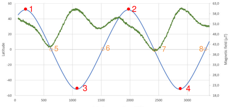
Team DAHspace from Portugal measured the intensity of the Earth’s magnetic field along the orbit path of the ISS. Using the magnetometer on the Astro Pi, their experiment recorded data allowing the team to track changes of intensity. The team mapped this data to the ISS’s coordinates, showing the difference in the Earth’s magnetic field between the North Pole (points 1 and 2 on the chart below) and the South Pole (points 3 and 4).
And the winning teams are…
We and our collaborators at ESA Education have been busy reviewing all of the reports to assess the scientific merit, use of the Astro Pi hardware, experiment design, and data analysis. The ten winning teams come from schools and coding clubs in 11 countries. We are sending each team some cool space swag to recognise their achievement.
Winning teams
| Team | Experiment theme | Based at | Country |
| Magnet47 | Life on Earth | O’Neill CVI | Canada |
| Aretusa | Life on Earth | Liceo Da Vinci Floridia | Italy |
| ASaether | Life on Earth | “Andrei Saguna” National College | Romania |
| Barrande | Life on Earth | Gymnázium Joachima Barranda Beroun | Czech Republic |
| Escapers | Life in space | Code Club | Canada |
| Futura | Life in space | Scuola Svizzera Milano | Italy |
| StMarks | Life on Earth | St Mark’s Church of England School | United Kingdom |
| DAHspace | Life on Earth | EB 2,3 D. Afonso Henriques | Portugal |
| T5Clouds | Life on Earth | Dominican College | Ireland |
| PiNuts | Life in space | TEKNISK GYMNASIUM, Skanderborg | Denmark |
You can click on a team name to read the team’s experiment report.
Highly commended teams
Along with the winning teams, we would like to commend the following teams for their experiments:
| Team | Experiment theme | Based at | Country |
| Parsec | Life on Earth | Liceo Da Vinci Pascoli Gallarate | Italy |
| Celeste | Life on Earth | International School of Florence | Italy |
| LionTech | Life on Earth | Colegiul Național ”Mihai Eminescu” | Romania |
| OHSpace | Life in Space | Oxford High School | United Kingdom |
| Magneto | Life on Earth | The American School of The Hague | Netherlands |
| GreenEye | Life on Earth | ROBOTONIO | Greece |
| Primus | Life on Earth | Independent coding club | Germany |
You can click on a team name to read the team’s experiment report.
All of the teams whose Mission Space Lab programs ran on the ISS will receive a certificate signed by ESA astronaut Samantha Cristoforetti. The winning and highly commended teams will also be invited to a live video chat with an ESA astronaut in the autumn.


Congratulations to all 2022/23 participants
Huge congratulations to every team that participated in Astro Pi Mission Space Lab. We hope you found it fun and inspiring to take part.
A big thank you to everyone who has been involved in the European Astro Pi Challenge this year. An amazing 24,850 young people from 29 countries had their programs run in space this year. We can’t wait to do it all again starting in September.
And it’s not just us saying thanks and well done — here’s a special message from ESA astronaut Matthias Maurer:
Looking forward to the next Astro Pi Challenge
On 18 September 2023, we’ll launch the European Astro Pi Challenge for 2023/24. Mission Zero will open in September, and we’ll announce exciting news about Mission Space Lab in September too.

If you know a young person who might be interested in the Astro Pi Challenge, sign up for the newsletter on astro-pi.org and follow the Astro Pi Twitter account for all the latest announcements about how you can support them to take the unique opportunity to write code to run in space.
The post Young people’s amazing experiments in space: Astro Pi Mission Space Lab 2022/23 appeared first on Raspberry Pi Foundation.
Fireflies
Post Syndicated from original https://xkcd.com/2802/

AlmaLinux to diverge (slightly) from RHEL
Post Syndicated from original https://lwn.net/Articles/938165/
AlmaLinux has announced that
the distribution will no longer be a strict clone of Red Hat Enterprise
Linux, but will maintain ABI compatibility.
For a typical user, this will mean very little change in your use
of AlmaLinux. Red Hat-compatible applications will still be able to
run on AlmaLinux OS, and your installs of AlmaLinux will continue
to receive timely security updates. The most remarkable potential
impact of the change is that we will no longer be held to the line
of “bug-for-bug compatibility” with Red Hat, and that means that we
can now accept bug fixes outside of Red Hat’s release cycle. While
that means some AlmaLinux OS users may encounter bugs that are not
in Red Hat, we may also accept patches for bugs that have not yet
been accepted upstream, or shipped downstream.
Mixing AWS Graviton with x86 CPUs to optimize cost and resiliency using Amazon EKS
Post Syndicated from Macey Neff original https://aws.amazon.com/blogs/compute/mixing-aws-graviton-with-x86-cpus-to-optimize-cost-and-resilience-using-amazon-eks/
This post is written by Yahav Biran, Principal SA, and Yuval Dovrat, Israel Head Compute SA.
This post shows you how to integrate AWS Graviton-based Amazon EC2 instances into an existing Amazon Elastic Kubernetes Service (Amazon EKS) environment running on x86-based Amazon EC2 instances. Customers use mixed-CPU architectures to enable their application to utilize a wide selection of Amazon EC2 instance types and improve overall application resilience. In order to successfully run a mixed-CPU application, it is strongly recommended that you test application performance in a test environment before running production applications on Graviton-based instances. You can follow AWS’ transition guide to learn more about porting your application to AWS Graviton.
This example shows how you can use KEDA for controlling application capacity across CPU types in EKS. KEDA will trigger a deployment based on the application’s response latency as measured by the Application Load Balancer (ALB). To simplify resource provisioning, Karpenter, an open-source Kubernetes node provisioning software, and AWS Load Balancer Controller, are shown as well.
Solution Overview
There are two solutions that this post covers to test a mixed-CPU application. The first configuration (shown in Figure 1 below) is the “A/B Configuration”. It uses an Application Load Balancer (ALB)-based Ingress to control traffic flowing to x86-based and Graviton-based node pools. You use this configuration to gradually migrate a live application from x86-based instances to Graviton-based instances, while validating the response time with Amazon CloudWatch.

Figure 1, config 1: A/B Configuration
In the second configuration, the “Karpenter Controlled Configuration” (shown in Figure 2 below as Config 2), Karpenter automatically controls the instance blend. Karpenter is configured to use weighted provisioners with values that prioritize AWS Graviton-based Amazon EC2 instances over x86-based Amazon EC2 instances.

Figure 2, config II: Karpenter Controlled Configuration, with Weighting provisioners topology
It is recommended that you start with the “A/B” configuration to measure the response time of live requests. Once your workload is validated on Graviton-based instances, you can build the second configuration to simplify the deployment configuration and increase resiliency. This enables your application to automatically utilize x86-based instances if needed, for example, during an unplanned large-scale event.
You can find the step-by-step guide on GitHub to help you to examine and try the example app deployment described in this post. The following provides an overview of the step-by-step guide.
Code Migration to AWS Graviton
The first step is migrating your code from x86-based instances to Graviton-based instances. AWS has multiple resources to help you migrate your code. These include AWS Graviton Fast Start Program, AWS Graviton Technical Guide GitHub Repository, AWS Graviton Transition Guide, and Porting Advisor for Graviton.
After making any required changes, you might need to recompile your application for the Arm64 architecture. This is necessary if your application is written in a language that compiles to machine code, such as Golang and C/C++, or if you need to rebuild native-code libraries for interpreted/JIT compiled languages such as the Python/C API or Java Native Interface (JNI).
To allow your containerized application to run on both x86 and Graviton-based nodes, you must build OCI images for both the x86 and Arm64 architectures, push them to your image repository (such as Amazon ECR), and stitch them together by creating and pushing an OCI multi-architecture manifest list. You can find an overview of these steps in this AWS blog post. You can also find the AWS Cloud Development Kit (CDK) construct on GitHub to help get you started.
To simplify the process, you can use a Linux distribution package manager that supports cross-platform packages and avoid platform-specific software package names in the Linux distribution wherever possible. For example, use:
RUN pip install httpd
instead of:
ARG ARCH=aarch64 or amd64
RUN yum install httpd.${ARCH}
This blog post shows you how to automate multi-arch OCI image building in greater depth.
Application Deployment
Config 1 – A/B controlled topology
This topology allows you to migrate to Graviton while validating the application’s response time (approximately 300ms) on both x86 and Graviton-based instances. As shown in Figure 1, this design has a single Listener that forwards incoming requests to two Target Groups. One Target Group is associated with Graviton-based instances, while the other Target Group is associated with x86-based instances. The traffic ratio associated with each target group is defined in the Ingress configuration.
Here are the steps to create Config 1:
- Create two KEDA
ScaledObjectsthat scale the number of pods based on the latency metric (AWS/ApplicationELB-TargetResponseTime) that matches the target group (triggers.metadata.dimensionValue). Declare the maximum acceptable latency intargetMetricValue:0.3.
Below is the Graviton deployment scaledObject (spec.scaleTargetRef), note the comments that denote the value of the x86 deployment scaledObject
apiVersion: keda.sh/v1alpha1
kind: ScaledObject
…
spec:
  scaleTargetRef:
    apiVersion: apps/v1
    kind: Deployment
    name: armsimplemultiarchapp #amdsimplemultiarchapp
…
  triggers:
    - type: aws-cloudwatch
      metadata:
        namespace: "AWS/ApplicationELB"
        dimensionName: "LoadBalancer"
        dimensionValue: "app/simplemultiarchapp/xxxxxx"
        metricName: "TargetResponseTime"
targetMetricValue: "0.3"- Once the topology has been created, add Amazon CloudWatch Container Insights to measure CPU, network throughput, and instance performance.
- To simplify testing and control for potential performance differences in instance generations, create two dedicated Karpenter provisioners and Kubernetes Deployments (replica sets) and specify the instance generation, CPU count, and CPU architecture for each one. This example uses c7g (Graviton3) and c6i (Intel) . You will remove these constraints in the next topology to allow more allocation flexibility.
The x86-based instances Karpenter provisioner:
apiVersion: karpenter.sh/v1alpha5
kind: Provisioner
metadata:
  name: x86provisioner
spec:
  requirements:
  - key: karpenter.k8s.aws/instance-generation
    operator: In
    values:
    - "6"
  - key: karpenter.k8s.aws/instance-cpu
    operator: In
    values:
    - "2"
  - key: kubernetes.io/arch
    operator: In
    values:
    - amd64
The Graviton-based instances Karpenter provisioner:
apiVersion: karpenter.sh/v1alpha5
kind: Provisioner
metadata:
  name: arm64provisioner
spec:
  requirements:
  - key: karpenter.k8s.aws/instance-generation
    operator: In
    values:
    - "7"
  - key: karpenter.k8s.aws/instance-cpu
    operator: In
    values:
    - "2"
  - key: kubernetes.io/arch
    operator: In
    values:
- arm64- Create two Kubernetes Deployment resources—one per CPU architecture—that use nodeSelector to schedule one Deployment on Graviton-based instances, and another Deployment on x86-based instances. Similarly, create two NodePort Service resources, where each Service points to its architecture-specific ReplicaSet.
- Create an Application Load Balancer using the AWS Load Balancer Controller to distribute incoming requests among the different pods. Control the traffic routing in the ingress by adding an ingress.kubernetes.io/actions.weighted-routing annotation. You can adjust the weight in the example below to meet your needs. This migration example started with a 100%-to-0% x86-to-Graviton ratio, adjusting over time by 10% increments until it reached a 0%-to-100% x86-to-Graviton ratio.
…
alb.ingress.kubernetes.io/actions.weighted-routing: |
{
…
  "targetGroups":[
    {
      "serviceName":"armsimplemultiarchapp-svc",
      "servicePort":"80","weight":50
    },
    {
      "serviceName":"amdsimplemultiarchapp-svc",
      "servicePort":"80","weight":50}]
    }
 }

spec:
  ingressClassName: alb
  rules:
    - http:
        paths:
          - path: /
            pathType: Prefix
            backend:
              service:
                name: weighted-routing
You can simulate live user requests to an example application ALB endpoint. Amazon CloudWatch populates ALB Target Group request/second metrics, dimensioned by HTTP response code, to help assess the application throughput and CPU usage.
During the simulation, you will need to verify the following:
- Both Graviton-based instances and x86-based instances pods process a variable amount of traffic.
- The application response time (p99) meets the performance requirements (300ms).
The orange (Graviton) and blue (x86) curves of HTTP 2xx responses (figure 4) show the application throughput (HTTP requests/seconds) for each CPU architecture during the migration.

Figure 3 HTTP 2XX per CPU architecture
Figure 4 shows an example of application response time during the transition from x86-based instances to Graviton-based instances. The latency associated with each instance family grows and shrinks as the live request simulation changes the load on the application. In this example, the latency on x86 instances (until 07:00) grew up to 300ms because most of the request load was directed at to x86-based pods. It began to converge at around 08:00 when more pods were powered by Graviton-based instances. Finally, after 15:00, the request load was processed by Graviton-based instances entirely.

Figure 4: Target Response Time p99
Config 2 – Karpenter Controlled Configuration
After fully testing the application on Graviton-based EC2 instances, you are ready to simplify the deployment topology with weighted provisioners while preserving the ability to launch x86-based instances as needed.
Here are the steps to create Config 2:
- Reuse the CPU-based provisioners from the previous topology, but assign a higher
.spec.weightto Graviton-based instances provisioner. The x86 provisioner is still deployed in case x86-based instances are required. Thekarpenter.k8s.aws/instance-familycan be expanded beyond those set in Config 1 or excluded by switching the operator toNotIn.
The x86-based Amazon EC2 instances Karpenter provisioner:
apiVersion: karpenter.sh/v1alpha5
kind: Provisioner
metadata:
  name: x86provisioner
spec:
  requirements:
  - key: kubernetes.io/arch
    operator: In
    values: [amd64]
The Graviton-based Amazon EC2 instances Karpenter provisioner:
apiVersion: karpenter.sh/v1alpha5
kind: Provisioner
metadata:
  name: priority-arm64provisioner
spec:
  weight: 10
  requirements:
  - key: kubernetes.io/arch
    operator: In
    values: [arm64]
- Next, merge the two Kubernetes deployments into one deployment similar to the original before migration (i.e., no specific nodeSelector that points to a CPU-specific provisioner).
The two services are also combined into a single Kubernetes service and the actions.weighted-routing annotation is removed from the ingress resources:
spec:
  rules:
    - http:
        paths:
          - path: /app
            pathType: Prefix
            backend:
              service:
                name: simplemultiarchapp-svc
- Unite the two KEDA ScaledObject resources from the first configuration and point them to a single deployment, e.g.,
simplemultiarchapp. The new KEDA ScaledObject will be:
apiVersion: keda.sh/v1alpha1
kind: ScaledObject
metadata:
  name: simplemultiarchapp-hpa
  namespace: default
spec:
  scaleTargetRef:
    apiVersion: apps/v1
    kind: Deployment
    name: simplemultiarchapp
…
Figure 5 Config 2 – Weighting provisioners results
A synthetic limit on Graviton CPU capacity is set to illustrate the scaling to x86_64 CPUs (Provisioner.limits.resources.cpu). The total application throughput (figure 6) is shown by aarch64_200 (blue) and x86_64_200 (orange). Mixing CPUs did not impact the target response time (Figure 6). Karpenter behaved as expected: prioritizing Graviton-based instances, and bursting to x86-based Amazon EC2 instances when CPU limits were crossed.

Figure 6 Config 2 -HTTP response time p99 with mixed-CPU provisioner
Conclusion
The use of a mixed-CPU architecture enables your application to utilize a wide selection of Amazon EC2 instance types and improves your applications’ resilience while meeting your service-level objectives. Application metrics can be used to control the migration with AWS ALB Ingress, Karpenter, and KEDA. Moreover, AWS Graviton-based Amazon EC2 instances can deliver up to 40% better price performance than x86-based Amazon EC2 instances. Learn more about this example on GitHub and more announcements about Gravtion.
Create a comprehensive view of AWS support cases with Amazon QuickSight
Post Syndicated from Yash Bindlish original https://aws.amazon.com/blogs/big-data/create-a-comprehensive-view-of-aws-support-cases-with-amazon-quicksight/
AWS customers are looking for an efficient tracking method of support cases raised with AWS Support across their multiple interconnected accounts. Having a unified view lets the cloud operations team derive actionable insights across the support cases raised by different business units and accounts. This helps ensure that the team has a comprehensive understanding of the state of existing support cases and can quickly identify and work with teams to resolve them. The team can also prioritize their responses based on the severity of impact of the issues and take action on cases that need acknowledgement or additional information. AWS Systems Manager is the operations hub for your AWS applications and resources and a secure end-to-end management solution for hybrid cloud environments that enables secure operations at scale. AWS Systems Manager Explorer provides a summary of support cases across your AWS accounts to help you get better visibility into the operational health of your AWS environment.
This post describes how Amazon QuickSight dashboards can help you visualize your support cases in a single pane of glass using data extracts from Systems Manager. QuickSight meets varying analytic needs from the same source of truth through modern interactive dashboards, paginated reports, embedded analytics, and natural language queries.
Solution overview
The following architecture diagram illustrates the use of Systems Manager to provide a summary of support cases across your AWS accounts. The solution automates the collection process using a Systems Manager Automation document, scheduling automations within a maintenance window. When the Systems Manager configuration is done, the automation extracts the all support cases across the organization and creates a CSV file in an Amazon Simple Storage Service (Amazon S3) bucket. From the S3 bucket, we integrate with Amazon Athena to create a table, and lastly we visualize all support cases in QuickSight. Note that for aggregating data across multiple accounts, they must reside within a single AWS Organization. Implementing the solution requires the following steps:
- Set up a Systems Manager maintenance window.
- Register an automation task in the maintenance window.
- Create a database in the AWS Glue Data Catalog.
- Create a custom classifier for an AWS Glue crawler.
- Create and run an AWS Glue crawler.
- Create views in Athena.
- Visualize AWS support cases in QuickSight.

Prerequisites
Before you get started, complete the following prerequisites:
- Have a Business or Enterprise support plan for your AWS accounts.
- Enable and set up Athena.
- Enable QuickSight in your data collection account. For instructions, refer to Setting up for Amazon QuickSight.
- Create an S3 bucket where Systems Manager Automation will export support cases.
- Follow the steps in Centralized view of support cases opened from multiple AWS accounts using AWS Systems Manager to establish Systems Manager Explorer and create a resource data sync for data aggregation.
- Create an Amazon Simple Notification Service (SNS) topic. Use the following command to create an SNS topic named
SSM-supportcases-notificationand subscribe an email address:
You should see the following output:
For more information, refer to Creating an Amazon SNS topic.
- Have an AWS Identity and Access Manager (IAM) Systems Manager Explorer Exporting OpsData role. The role
AmazonSSMExplorerExportallows Explorer to export OpsData to a CSV file. For more information, refer to Exporting OpsData from Systems Manager Explorer. - Have Systems Manager permissions for maintenance windows. For more information, refer to Use the console to configure permissions for maintenance windows.
After you have all the prerequisites in place, follow the step-by-step instructions in the rest of this post.
Set up a Systems Manager maintenance window
Maintenance windows, a capability of Systems Manager, help you define a schedule for AWS support cases to extract at a predefined schedule. For instructions on creating a maintenance window, see Create a maintenance window (console).

Register an automation task with a maintenance window
In this step, you add a task to a maintenance window. Tasks are the actions performed when a maintenance window runs. For instructions on registering an automation task to a maintenance window, see Schedule automations with maintenance windows.
- Provide a name for the maintenance task and choose the automation document
AWS-ExportOpsDataToS3

2. Enter the following details in the Input parameters section.
| Variable | Description | Value |
assumeRole |
(Required) The role ARN to assume during the automation run | The role you created as a prerequisite |
filters |
(Optional) Filters for the getOpsSummary request |
Leave blank |
syncName |
(Optional) The name of the resource data sync | The sync name that you created as a prerequisite |
resultAttribute |
(Optional) The result attribute for the getOpsSummary request |
AWS:SupportCenterCase |
columnFields |
(Optional) The column fields to write to the output file | “DisplayId”,”SourceAccountId”,”Subject”,”Status”,”ServiceCode”,”CategoryCode”,”SeverityCode”,”TimeCreated” |
s3BucketName |
(Required) The S3 bucket where you want to download the output file | The S3 bucket that you created as a prerequisite |
snsTopicArn |
(Required) The SNS topic ARN to notify when the download is complete | The ARN for the SNS topic that you created as a prerequisite |
snsSuccessMessage |
(Optional) The message to send when a document is complete | Leave blank |
columnFieldsWithType |
(Optional) The fully qualified column fields to write to the output file | Leave blank |
resultAttributeList |
(Optional) The multiple result attributes for the getOpsSummary request |
Leave blank |

- Choose the IAM service role you created as a prerequisite.
- Choose Register Automation task.

After you successfully register the task, the automation will run, and you will see CSV files getting created in your S3 bucket. In our use case, we set the rate expression as 1 day. However, you can use a lesser frequency such as 1 hour or even 5 minutes to test the functionality.

Create a database in the AWS Glue Data Catalog
Before you can create an AWS Glue crawler, you need to create a database in the Data Catalog, which is a container that holds tables. You use databases to organize your tables into separate categories. In our use case, support cases data resides in an S3 bucket.
- On the AWS Glue console, create a new database.
- For Name, enter a name (for example,
aws_support_cases). - Add an optional location and description.
- Choose Create database.
For more information about AWS Glue databases, refer to Working with databases on the AWS Glue console.

Create a custom classifier
Crawlers invoke classifiers to infer the schema of your data. We need to create a custom classifier because when we extract the support cases, every column in a potential header parses as a string data type. When creating your classifier, choose Has headings and add the following:
For more information on classifiers, refer to Adding classifiers to a crawler in AWS Glue.

Create an AWS Glue crawler
To create a crawler that reads files stored on Amazon S3, complete the following steps:
- On the AWS Glue console, in the navigation pane, choose Crawlers.
- On the Crawlers page, choose Add crawler.
- For Crawler name, enter support cases extract, then choose Next.
- For the crawler source type, choose Data stores, then choose Next.
Now let’s point the crawler to your data.
- On the Add a data store page, choose the Amazon S3 data store.
- For Crawl data in, choose Specified path in this account.
- For Include path, enter the path where the crawler can find the support cases data, which is
s3://S3_BUCKET_PATH. After you enter the path, the title of this field changes to Include path. - Choose Next.
The crawler also needs permissions to access the data store and create objects in the Data Catalog.
- To configure these permissions, choose Create an IAM role. The IAM role name starts with
AWSGlueServiceRole-; you enter the last part of the role name (for this post, we enterCrawlercases). - Choose Next.
Crawlers create tables in your Data Catalog. Tables are contained in a database in the Data Catalog.
- Choose Target database and select the database you created.
Now we create a schedule for the crawler.
- For Frequency, choose Daily
- Choose Next.
- Verify the choices you made. If you see any mistakes, you can choose Edit to return to previous pages and make changes.
- After you have reviewed the information, choose Finish to create the crawler.
For more information on creating an AWS Glue crawler, refer to Adding an AWS Glue crawler.

Create views in Athena
After the AWS Glue crawler is configured successfully, we query the data from the database and table created by the crawler and create views in Athena. The data source for the dashboard will be an Athena view of your existing support_cases database. We create a view in Athena with a group by condition.

Create the view case_summary_view by modifying the table name support_cases from the following code and run the query in the Athena query editor:
Visualize AWS support cases in QuickSight
After we create the Athena view, we can create a dashboard in QuickSight. Before connecting QuickSight to Athena, make sure to grant QuickSight access to Athena and the associated S3 buckets in your account. For details, refer to Authorizing connections to Amazon Athena.
- On the QuickSight console, choose Datasets in the navigation pane.
- Choose New dataset.

- Choose Athena as your data source.
- For Data source name¸ enter
AWS_Support_Cases. - Choose Create data source.

- For Database, choose the
aws_support_casesdatabase, which contains the views you created (refer to the Athena console if you are unsure which ones to select) - For Tables, select the
case_summary_viewtable that we created as part of the steps in Athena. - Choose Edit/Preview data.

- Select SPICE to change your query mode.


Now you can create the sheet aws_support_cases in the analysis.
- Choose Publish & Visualize.
- Select the sheet type that you want (Interactive sheet or Paginated report). For this post, we select Interactive sheet.
- Choose Add.

Refer to Starting an analysis in Amazon QuickSight for more information about creating an analysis.
- In Sheet 1 of the newly created analysis, under Fields list, choose
case_categoryandcase_status. - For Visual types, choose a clustered bar combo chart.
This type of visual returns the count of records by case category.

- To add more visuals to the workspace, choose Add, then Add visual.
In the second visual, we create a donut chart with the field case_status to count the number of overall cases.

- Next, we create a word cloud to display how often AWS support cases have been raised by which AWS account.
The word cloud shows the top 100 accounts by default (if you have data for more than one account) and displays the account with the maximum number of entries in a higher font size. If you wanted to show just the top account, you would have to configure a top 1 filter.

- Next, we create a stacked bar combo chart to display cases with service type, using the fields
case_created_on,caseid, andcase_service. - Next, we create a table visual to display all case details in table format (select all available fields).

The following screenshot shows a visualization of all fields of support cases in tabular format.
19. Adjust the size and position of the visuals to fit the layout of your analysis.

The following screenshot shows our final dashboard for support cases.

You’ve now set up a fully functional AWS support cases dashboard at an organizational view. You can share the dashboard with your cloud platform and operations teams. For more information, refer to Sharing Amazon QuickSight dashboards.
Clean up
When you don’t need this dashboard anymore, complete the following steps to delete the AWS resources you created to avoid ongoing charges to your account:
- Delete the Amazon S3 Bucket
- Delete the SNS topic.
- Delete the IAM roles.
- Cancel your QuickSight subscription. You should only delete your QuickSight account if you explicitly set it up to follow this post and are absolutely sure that it’s not being used by any other users.
Conclusion
This post outlined the steps and resources required to construct a customized analytics dashboard in QuickSight, empowering you to attain comprehensive visibility and valuable insights into support cases generated across multiple accounts within your organization. To learn more about how QuickSight can help your business with dashboards, reports, and more, visit Amazon QuickSight.
About the authors
 Yash Bindlish is a Enterprise Support Manager at Amazon Web Services. He has more than 17 years of industry experience including roles in cloud architecture, systems engineering, and infrastructure. He works with Global Enterprise customers and help them build, scalable, modern and cost effective solutions on their growth journey with AWS. He loves solving complex problems with his solution-oriented approach.
 Shivani Reddy is a Technical Account Manager (TAM) at AWS with over 12 years of IT experience. She has worked in a variety of roles, including application support engineer, Linux systems engineer, and administrator. In her current role, she works with global customers to help them build sustainable software solutions. She loves the customer management aspect of her job and enjoys working with customers to solve problems and find solutions that meet their specific needs.
New – Amazon FSx for NetAPP ONTAP Now Supports WORM Protection for Regulatory Compliance and Ransomware Protection
Post Syndicated from Jeff Barr original https://aws.amazon.com/blogs/aws/new-amazon-fsx-for-netapp-ontap-now-supports-worm-protection-for-regulatory-compliance-and-ransomware-protection/
Amazon FSx for NetApp ONTAP was launched in late 2021. With FSx for ONTAP you get the popular features, performance, and APIs of ONTAP file systems, with the agility, scalability, security, and resilience of AWS, all as a fully managed service.
Today we are adding support for SnapLock, an ONTAP feature that gives you the power to create volumes that provide Write Once Read Many (WORM) functionality. SnapLock volumes prevent modification or deletion of files within a specified retention period, and can be used to meet regulatory requirements and to protect business-critical data from ransomware attacks and other malicious attempts at alteration or deletion. FSx for ONTAP is the only cloud-based file system that supports SnapLock Compliance mode. FSx for ONTAP also supports tiering of WORM data to lower-cost storage for all SnapLock volumes.
Protecting Data with SnapLock
SnapLock gives you an additional layer of data protection, and can be thought of as part of your organization’s overall data protection strategy. When you create a volume and enable SnapLock, you choose one of the following retention modes:
Compliance – This mode is used to address mandates such as SEC Rule 17a-4(f), FINRA Rule 4511 and CFTC Regulation 1.31. You can use this mode to ensure a WORM file cannot be deleted by any user until after its retention period expires. Volumes in this mode cannot be renamed and cannot be deleted until the retention periods of all WORM files on the volume have expired.
Enterprise – This mode is used to enforce organizational data retention policies or to test retention settings before creating volumes in Compliance mode. You can use this mode to prevent most users from deleting WORM data, while allowing authorized users to perform deletions, if necessary. Volumes in this mode can be deleted even if they contain WORM files under an active retention period.
You also choose a default retention period. This period indicates the length of time that each file must be retained after it is committed to the WORM state, and can be as long as 100 years, and there’s also an Infinite option. You can also set a custom retention period for specific files or specific trees of files and it will apply to those files at the time that they are committed to the WORM state.
Files are committed to the WORM state when they become read-only (chmod -w on Linux or attrib +r on Windows). You can configure a per-volume autocommit period (5 minutes to 10 years) to automatically commit files that have remained as-is for the period, and you can also initiate a Legal Hold in Compliance mode in order to retain specific files for legal purposes.
You also have another interesting data protection and compliance option. You can create one volume without SnapLock enabled, and another one with it enabled, and then periodically replicate from the first one to the second using NetApp SnapVault. This will give you snapshot copies of entire volumes that you can retain for months, years, or decades as needed.
Speaking of interesting options, you can make use of FSx for ONTAP volume data tiering to keep active files on high-performance SSD storage and the other files on storage that is cost-optimized for data that is accessed infrequently.
Creating SnapLock Volumes
I can create new volumes and enable SnapLock with a couple of clicks. I enter the volume name, size, and path as usual:
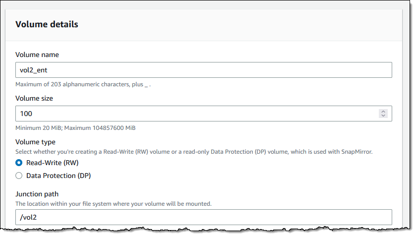
As I mentioned earlier, I can also make use of a capacity pool (this is set to Auto by default, and I set a 10 day cooling period):
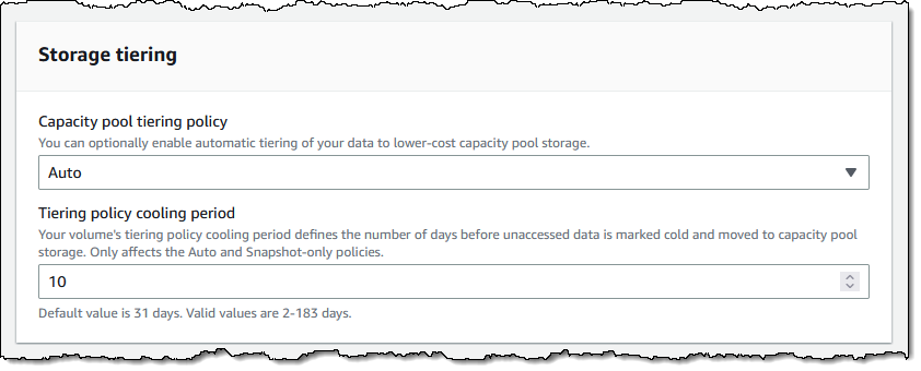
I scroll down to the Advanced section and click Enabled, then select Enterprise retention mode. I also set up my retention periods, enable autocommit after 9 days, and leave the other options as-is:

I add a tag, and click Create volume to move ahead:

I take a quick break, and when I come back my volume is ready to use:

At this point I can mount it in the usual way, create files, and allow SnapLock to do its thing!
Things to Know
Here are a couple of things that you should know about this powerful new feature:
Existing Volumes – You cannot enable this feature for an existing volume, but you can create a new, SnapLock-enabled volume, and copy or migrate the data to it.
Volume Deletion – As I noted earlier, you cannot delete a SnapLock Compliance volume if it contains WORM files with an unexpired retention period. Take care when setting this to avoid creating volumes that will last longer than needed.
Pricing – There’s an additional GB/month license charge for the use of SnapLock volumes; check out the Amazon FSx for NetAPP ONTAP Pricing page for more information.
Regions – This feature is available in all AWS Regions where Amazon FSx for NetApp ONTAP is available.
— Jeff;
Meross Outdoor Smart Plug or Smart Power Strip?
Post Syndicated from BeardedTinker original https://www.youtube.com/watch?v=huXLIHs4pC0
Pentales: Old Vulns, New Tricks
Post Syndicated from Austin Guidry original https://blog.rapid7.com/2023/07/13/pentales-old-vulns-new-tricks/

At Rapid7 we love a good pentest story. So often they show the cleverness, skill, resilience, and dedication to our customer’s security that can only come from actively trying to break it! In this series, we’re going to share some of our favorite tales from the pen test desk and hopefully highlight some ways you can improve your own organization’s security.
This engagement began like any other Internal Network Penetration test. I followed a systematic methodology to enumerate the internal domain. The target organization was a financial institution, but their internal domain was administered via Active Directory (AD) like most organizations with more than a handful of computers. AD is a Microsoft product that provides centralized control of the whole gamut of networking devices that an organization may have. This may include workstations, servers, switches, routers, printers, and IoT devices. Additionally, AD can be used for localized, global, or cloud-based networks.
After enumeration, I identified high value targets and a wide range of open ports and services. I used a Metasploit RC file containing instructions and settings to configure Metasploit modules. This allowed me to scan the open ports and services for common/default credentials, vulnerabilities, misconfigurations, software types, version numbers, and other accessible information in the background while I covered more ground manually.
I began operations to understand the state of several types of combinable networking vulnerabilities, checking for broadcast name services (BNS) and poisoning capabilities, Server Message Block (SMB) Signing statuses for hosts using SMB visible to my attack box (PTK), and for Internet Protocol version 6 (IPv6) traffic. These are some of the more common ways to begin a successful attack path. I checked all of these options on this organization’s network, but I found that I could not leverage BNS poisoning, SMB Signing not required, or IPv6-based attacks.
Luckily, the Metasploit RC file found default credentials for Intelligent Platform Management Interface (IPMI) assets. The IPMI protocol’s design introduced a vulnerability that provides a hash to someone attempting authentication. A user would attempt to authenticate with a specific username, and the IPMI device would provide the hash for that account. The Metasploit module for dumping IPMI hashes does this exactly for a wordlist full of common usernames and checks the provided hashes against a partial rainbow table of common passwords like “admin” and “root.” In this case, several devices were using credentials such as “admin:admin” and “root:root.”
This is exciting because IPMI is used to control servers, and more often these days server virtualization is such that several server virtual machines (VMs) are hosted on one physical server computer. I logged into the web interfaces associated with these IPMIs and found within the remote consoles that three of these IPMI assets were hosting VMware ESXi instances. VMware ESXi is, in fact, used to host and manage multiple VMs. The remote consoles provided the IP and website addresses for the VMware ESXi administrative login interfaces. I navigated to these interfaces and typed in the default credentials used on the IPMI hosts… and they were valid!
At this point, I was quite shocked that default credentials were in use, some 4+ decades after “admin:admin” became an official vulnerability. Not to mention, default credentials to valuable assets is probably the simplest and easiest vulnerability to exploit.
So, I got into the VMware ESXi consoles and I quickly identified which of the three assets contained the primary Domain Controller (DC) and Exchange Server. As an administrator to the VMware ESXi console, I had a lot of flexibility in what I was able to do with the virtual machines. First, I checked to see if there were sessions still open with these two assets. Both were locked and would require valid credentials to access via (Remote Desktop Protocol) RDP or similar remote access control.
I could conduct other attacks such as Denial of Service (DoS), deleting the machine or turning it off, but this would immediately be noticed by organization personnel, and most importantly these types of attacks were out of scope. DoS is out of scope for pentesters by default. This type of attack is extremely harmful to business operations, and has the potential to cause irreversible harm.
I needed to find an interface with which I had administrative control to view data on these VMs vs. trying to use the underlying Operating Systems (OS) within the VMs. I tried to download the VMs, but they would have taken 10 + days for the DC and multiple weeks for the Exchange Server. I tried to create a snapshot of the memory of the DC to attempt to filter credentials from it, but this was also too large and I could not acquire the file during the engagement.
I asked for help from the consulting team. At Rapid7, we have a deep bench of talented and knowledgeable people and a healthy culture of teamwork and support.
One of my teammates hopped on a call to help me investigate the potential options. Upon further review of the accessible ports and services in use by the VMware ESXi host, we found that Secure Shell (SSH) was open and accessible. There is a tool called SSHFS, which stands for SSH File System. This tool uses an SSH connection to mount and interact with the files on a remote device. This is similar to Network File Share (NFS) where a user can create a directory and mount it to the directory of a remote device. With administrative credentials to the VMware ESXi device, this provided me administrative control over the remote system’s file system and allowed me to interact with it in the same way as local files.
From here, I simply navigated to the directory within the DC that contained the NTDS.DIT file. This file is present on all Windows hosts, however, when it is contained by a Domain Controller this file contains all of the New Technology LAN Manager (NTLM) hashes for all of the accounts on the domain, including users, workstation machine accounts, and service accounts.
Sometimes, for environments that have or once had devices older than Windows Vista or Server 2008, there are also LM hashes which are incredibly weak. The entire keyspace for LM can be cracked in minutes to hours depending on the hardware, and the entire 8 character keyspace for NTLM can be cracked within several hours on enterprise-grade hardware.
This does not even cover the most valuable feature of NTLM authentication. NTLM hashes can be used as passwords, making it irrelevant to know the cleartext password that created the hash. This is called a “pass-the-hash” attack. Upon successfully dumping the NTDS.DIT file for the organization’s domain, I now controlled every domain-joined account and device.
With this control, I switched gears to post-exploitation and demonstrating impact for the organization’s stakeholders. I logged into several email accounts, looking for and finding sensitive information such as Social Security Numbers (SSNs) and Account Numbers. I sent emails from organizational personnel’s email accounts to the point-of-contact and myself, demonstrating the impersonation potential. I used cracked account credentials to locate accounts for which Multi-factor Authentication (MFA) had not been configured and enrolled in MFA for one account. I perused several organization-wide network file share servers finding sensitive documents, PII, account numbers, bank and loan statements, and network information. I found multiple PDFs identifying the organization’s ATMs, their names, locations, makes and models, support information from supporting third-parties, and IP addresses.
I used these ATM IP addresses to conduct additional enumeration attempting to discover attack paths to gain control of ATMs. I found several open ports but was unable to gain access or control to the ATMs. However, within the directories containing ATM information were Excel spreadsheet logs of ATM activity. These non-password-protected spreadsheets held cardholder data, their links to bank customer account numbers, and historical information such as timestamps, locations, transaction amounts, and transaction types.
The customer’s environment had a lot of time and effort dedicated to security, and the security team covered many of the “low-hanging-fruit.” Sometimes older technology like IPMI is necessary for business. It is vital to understand the risks and to work with the technology we have to secure it against well-documented attacks. Why allow anyone internally to see an administrative resource? Access controls and closing unnecessary ports could minimize the attack surface on exploitable systems. Finally, one of the best defenses continues to be a strong, unique password for all logins, local or domain.
We, the pentesters at Rapid7 put our experience and knowledge together to reveal the weaknesses in the customer’s environment and give them the opportunities to fix them. Sometimes hacking is like finding a needle in the haystack, but we hackers have automated needle-finding, haystack-searching machines. Do your research, do the best you can, and when in doubt, get a pentest!
Check us out at this year’s Black Hat USA in Las Vegas! Our experts will be giving talks and our booth will be staffed with many members of our team. Stop by and say hi.
Old Blackmoon Trojan, NEW Monetization Approach
Post Syndicated from Natalie Zargarov original https://blog.rapid7.com/2023/07/13/old-blackmoon-trojan-new-monetization-approach/

Rapid7 is tracking a new, more sophisticated and staged campaign using the Blackmoon trojan, which appears to have originated in November 2022. The campaign is actively targeting various businesses primarily in the USA and Canada. However, it is not used to steal credentials, instead it implements different evasion and persistence techniques to drop several unwanted programs and stay in victims’ environment for as long as possible.
Blackmoon, also known as KRBanker, is a banking trojan first spotted in late September 2015 when targeting banks of the Republic of Korea. Back in 2015, it was using a “pharming” technique to steal credentials from targeted victims. This technique involves redirecting traffic to a forged website when a user attempts to access one of the banking sites being targeted by the cyber criminals. The fake server masquerades the original site and urges visitors to submit their information and credentials.
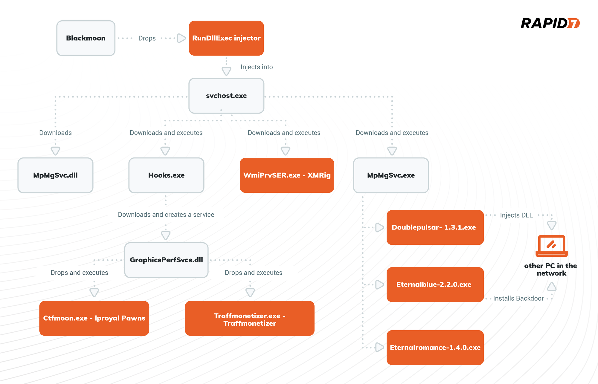
Stage 1 – Blackmoon
Blackmoon trojan was named after a debug string “blackmoon,” that is present in its code:

Blackmoon drops a dll into C:\Windows\Logs folder named RunDllExe.dll and implements a Port Monitors persistence technique. Port Monitors is related to the Windows Print Spooler Service or spoolsv.exe. When adding a printer port monitor a user (or the attacker in our case) has the ability to add an arbitrary dll that acts as the monitor. There are two ways to add a port monitor: via Registry for persistence or via a AddMonitor API call for immediate dll execution.
Our sample implements both, it calls AddMonitor API call to immediately execute RunDllExe.dll:

It also sets a Driver value in HKLM\SYSTEM\CurrentControlSet\Control\Print\Monitors\RunDllExe registry key to the malicious dll path.

Next, the malware adds a shutdown system privilege to the Spooler service by adding SeShutdownPrivilege to the RequiredPrivileges value of HKEY_LOCAL_MACHINE\SYSTEM\CurrentControlSet\Services\Spooler registry key.


The malware disables Windows Defender by setting HKLM\SOFTWARE\Policies\Microsoft\Windows Defender\DisableAntiSpyware value to “1”.
It also stops and disables “Lanman” service (the service that allows a computer to share files and printers with other devices on the network).
To block all incoming RPC and SMB communication the malware executes the set of following commands:
netsh ipsec static add policy name=Block
netsh ipsec static add filterlist name=Filter1
netsh ipsec static add filter filterlist=Filter1 srcaddr=any dstaddr=Me dstport=135 protocol=TCP
netsh ipsec static add filter filterlist=Filter1 srcaddr=any dstaddr=Me dstport=135 protocol=UDP
netsh ipsec static add filter filterlist=Filter1 srcaddr=any dstaddr=Me dstport=139 protocol=TCP
netsh ipsec static add filter filterlist=Filter1 srcaddr=any dstaddr=Me dstport=139 protocol=UDP
netsh ipsec static add filter filterlist=Filter1 srcaddr=any dstaddr=Me dstport=445 protocol=TCP
netsh ipsec static add filter filterlist=Filter1 srcaddr=any dstaddr=Me dstport=445 protocol=UDP
netsh ipsec static add filteraction name=FilteraAtion1 action=block
netsh ipsec static add rule name=Rule1 policy=Block filterlist=Filter1 filteraction=FilteraAtion1
netsh ipsec static set policy name=Block assign=y
The malware sets two additional values under HKEY_LOCAL_MACHINE\SYSTEM\CurrentControlSet\Services\aspnet_staters: Work and Mining, both set to “1”.
Next, the malware checks if one of the following services exists on the victim computer:
- clr_optimization_v3.0.50727_32
- clr_optimization_v3.0.50727_64
- WinHelpsvcs
- Services
- Help Service
- KuGouMusic
- WinDefender
- Msubridge
- ChromeUpdater
- MicrosoftMysql
- MicrosoftMssql
- Conhost
- MicrosotMaims
- MicrosotMais
In case the service is found, it will be disabled (by setting “Start” value under HKEY_LOCAL_MACHINE\SYSTEM\CurrentControlSet\Services\servicename to “4”) or deleted by using DeleteService API call.
The malware enumerates running processes by using a combination of CreateToolhelp32Snapshot and Process32First and Process32Next API calls to terminate service’s process if one is running.
Finally, a Powershell command is executed to delete the running process’s file and the malware exits.
Stage 2 – RunDllExe.dll – injector
RunDllExe.dll is executed by Spooler service and is responsible for injecting a next stage payload into the newly executed svchost.exe process. The malware implements Process Hollowing injection technique. The injected code is a C++ file downloader.
Stage 3 – File Downloader
The downloader first checks if ‘Work’ and ‘Mining’ values exist and set under HKEY_LOCAL_MACHINE\SYSTEM\CurrentControlSet\Services\aspnet_staters registry key, if the values do not exist, it will create them and set both to “1”.
As downloader, this part of the attack flow is checking if all needed to be downloaded files are already present (by using PathFileExistsA API call) on the PC, if not, the malware sleeps for two minutes before every download and then use the URLDownloadToFileA API call to download the following files:
- C:\WINDOWS\Temp\MpMgSvc.dll
- C:\WINDOWS\Temp\Hooks.exe
- C:\WINDOWS\Temp\MpMgSvc.exe
- C:\Windows\Microsoft.NET\Framework\v3.0\WmiPrvSER.exe
After the download all but the MpMgSvc.dll are executed by the downloader:

Stage 4 – Hook.exe – dropper
Hook.exe drops an additional dll to the users roaming folder C:\Users\Username\AppData\Roaming\GraphicsPerfSvcs.dll and creates a new service named GraphicsPerfSvcs, which will be automatically executed at system startup. The service name is almost identical to the legitimate service named GraphicsPerfSvc, which belongs to the Graphics performance monitor service. Naming services and files similarly to the once belonged to OS is an evasion technique widely used by threat actors.

The dropper starts the created service. It then creates and executes a .vbs which responsible for deleting Hook.exe and the .vbs itself:

Stage 4.1 – MpMgSvc.exe – spreader MpMgSvc.exe first creates a new \BaseNamedObjects\Brute_2022 mutex. As being responsible for spreading the malware, it drops Doublepulsar-1.3.1.exe, Eternalblue-2.2.0.exe, Eternalromance-1.4.0.exe and all required for these files libraries into the C:\Windows\Temp folder.
Then it scans the network for PC’s with open 3306, 445, 1433 ports. If any open ports are found, the spreader will attempt to install a backdoor by using EternalBlue and send shellcode to inject dll with Doublepulsar as implemented in the Eternal-Pulsar github project .

There are two dlls dropped, one for x64 architecture and the second one for x86. When injected by Doublepulsar it will download the first stage Blackmoon malware and follow the same execution stages described in this analysis.
Stage 4.2 – WmiPrvSER.exe – XMRig miner
WmiPrvSER.exe is a classic XMRig Monero miner. Our sample is the XMRig version 6.18, and it creates a BaseNamedObjects\\Win__Host mutex on the victim’s host. You can find a full report on XMRig here.
Stage 5 – GraphicsPerfSvcs service – dropper
As mentioned in the previous stage, the GraphicsPerfSvcs service will be started automatically at system startup. Every time it runs, it will check if two of the following files exist:
- C:\Windows\TEMP\ctfmoon.exe
- C:\Windows\Microsoft.NET\traffmonetizer\Traffmonetizer.exe
If not found, it will drop both those files and all needed dlls for their execution.
The dropper also creates two new firewall rules that allow all outbound connections from dropped files by executing the following commands:
netsh advfirewall firewall add rule name=ctfmoon dir=out program=C:\Windows\Microsoft.NET\ctfmoon.exe action=allownetsh advfirewall firewall add rule name=traffmonetizer dir=out program=C:\Windows\Microsoft.NET\traffmonetizer\traffmonetizer.exe action=allow

The service stays up and constantly attempts to read from the URL: hxxp://down.ftp21[.]cc/Update.txt. At the time of the analysis, this URL was down so we were not able to observe its content. However, following the service code, it seems to read the URL content and check if it contains one of the following commands:
[Delete File], [Kill Proccess], or [Delete Service], which will delete file, kill process or delete service accordingly.
Stage 6 – Ctfmoon.exe and Traffmonetizer.exe – Traffic Stealers
GraphicsPerfSvcs service executes two dropped files: Ctfmoon.exe and Traffmonetizer.exe, both appeared to be Potentially Unwanted Programs (PUP’s) in the form of traffic stealers. Both software are using the “network bandwidth sharing” monetization scheme to make “passive income”.
Ctfmoon.exe is a cli version of the Iproyal Pawns application. It gets the user email address and password as execution parameters to associate the activity and collect the money to the passed account. GraphicsPerfSvcs executes the following command line to start the Iproyal Pawns: ctfmoon.exe [email protected] -password=123456Aa. -device-name=Win32 -accept-tos
We can see that the user mentioned in our execution parameters already made $169:

The Traffmonetizer.exe is similar to Ctfmoon.exe, created by Traffmonetizer. It reads the user account data from a settings.json file dropped in users roaming directory. Our .json file contains the following content:
{"Token":"1gUgURMzQiuGFgttIdjeZBS0G6fqFlVvhCKlqzfHd3o=","StartWithWindows":false,"Accepting":true}.
Conclusion
The analysis in this blog reveals the effort threat actors put into the attack flow, by using several evasion and persistence techniques and using different approaches to increase their income and use victim resources.
MITRE ATT&CK Techniques:
| Persistence | Boot or Logon Autostart Execution: Port Monitors (T1547.010) | The Blackmoon trojan (a95737adb2cd7b1af2291d143200a82d8d32 a868c64fb4acc542608f56a0aeda) is using Port Monitors technique to establish persistence on the target host. |
|---|---|---|
| Persistence | Create or Modify System Process: Windows Service (T1543.003) | The Hook.exe dropper (1A7A4B5E7C645316A6AD59E26054A95 654615219CC03657D6834C9DA7219E99F) creates a new service to establish persistence on the target host. |
| Defense Evasion | Process Injection: Process Hollowing (T1055.012) | The dll dropped by Blackmoon (F5D508C816E485E05DF5F58450D623DC6B FA35A2A0682C238286D82B4B476FBB) is using the process hollowing technique to evade endpoint security detection. |
| Defense Evasion | Impair Defenses: Disable or Modify Tools (T1562.001) | The Blackmoon trojan (a95737adb2cd7b1af2291d143200a82d8 d32a868c64fb4acc542608f56a0aeda) disables Windows Defender to evade end-point security detection. |
| Lateral Movement | Exploitation of Remote Services (T1210) | The MpMgSvc.exe spreader (72B0DA797EA4FC76BA4DB6AD131056257965D F9B2BCF26CE2189AF3DBEC5B1FC) uses EternalBlue and DoublePulsar to spread in organization’s environment. |
| Discovery | Network Share Discovery (T1135) | The MpMgSvc.exe spreader (72B0DA797EA4FC76BA4DB6AD131056257965D F9B2BCF26CE2189AF3DBEC5B1FC) scans the network do discover open SMB ports. |
| Impact | Resource Hijacking (T1496) | The XMRing miner (ECC5A64D97D4ADB41ED9332E4C0F5DC7DC02 A64A77817438D27FC31C69F7C1D3), Iproyal Pawns trafficStealer (FDD762192D351CEA051C0170840F1D8D 171F334F06313A17EBA97CACB5F1E6E1) and Traffmonetizer trafficStealer (2923EACD0C99A2D385F7C989882B7CCA 83BFF133ECF176FDB411F8D17E7EF265) executed to use victim’s resources. |
| Impact | Service Stop (T1489) | The Blackmoon trojan (a95737adb2cd7b1af2291d143200a82d8d 32a868c64fb4acc542608f56a0aeda) stops updates and security products services. |
| Command and Control | Application Layer Protocol: Web Protocols (T1071.001) | The downloader (E9A83C8811E7D7A6BF7EA7A656041BCD68968 7F8B23FA7655B28A8053F67BE99) downloads next stage payloads over HTTP protocol. GraphicsPerfSvcs service (5AF88DBDC7F53BA359DDC47C3BCAF3F5FE 9BDE83211A6FF98556AF7E38CDA72B) uses HTTP protocol to get command from C&C server. |
IOC’s
| File name | SHA-256 | |
|---|---|---|
| 445.exe | a95737adb2cd7b1af2291d143200a82 d8d32a868c64fb4acc542608f56a0aeda |
Blackmoon Trojan |
| RunDllExe.dll | F5D508C816E485E05DF5F58450D623DC 6BFA35A2A0682C238286D82B4B476FBB |
Injector |
| Injected code | E9A83C8811E7D7A6BF7EA7A656041BCD 689687F8B23FA7655B28A8053F67BE99 |
Downloader |
| MpMgSvc.dll | E9BD4A9C6EA27033BCB696E65D7441DC2D 42CD7F9F02084B5C704316F0A4FDDF |
|
| Hooks.exe | 1A7A4B5E7C645316A6AD59E26054A95654615 219CC03657D6834C9DA7219E99F |
Dropper |
| MpMgSvc.exe | 72B0DA797EA4FC76BA4DB6AD131056257965 DF9B2BCF26CE2189AF3DBEC5B1FC |
Spreader |
| WmiPrvSER.exe | ECC5A64D97D4ADB41ED9332E4C0F5DC7DC02 A64A77817438D27FC31C69F7C1D3 |
XMRig |
| GraphicsPerfSvcs.dll | 5AF88DBDC7F53BA359DDC47C3BCAF3F5FE9BDE 83211A6FF98556AF7E38CDA72B |
Dropper |
| Doublepulsar-1.3.1.exe | 15FFBB8D382CD2FF7B0BD4C87A7C0BFFD1541 C2FE86865AF445123BC0B770D13 |
Shellcode installer |
| Eternalblue-2.2.0.exe | 85B936960FBE5100C170B777E1647CE9F0F0 1E3AB9742DFC23F37CB0825B30B5 |
Exploit |
| Eternalromance-1.4.0.exe | B99C3CC1ACBB085C9A895A8C3510F6DAA F31F0D2D9CCB8477C7FB7119376F57B |
Exploit |
| X64.dll | 275A9A7B99F3474CBF8A61964A6022E3CF 7BAF76E0EE2FBA31A708D8F1E25BD0 |
shellcode |
| X86.dll | F247A48D3ECDBDF91FCD7A2D8728ADAAF 06149586ADDE62DE7212C6DE645AD58 |
shellcode |
| Ctfmoon.exe | FDD762192D351CEA051C0170840F1D8D171 F334F06313A17EBA97CACB5F1E6E1 |
Iproyal Pawns |
| Traffmonetizer.exe | 2923EACD0C99A2D385F7C989882B7CCA8 3BFF133ECF176FDB411F8D17E7EF265 |
Traffmonetizer |
| [email protected] | Iproyal Pawns account | |
| 1gUgURMzQiuGFgttIdjeZBS0 G6fqFlVvhCKlqzfHd3o= |
Traffmonetizer token |
|
| hxxp://down.ftp21[.]cc | C&C server |
References
How to Use Cloud Replication to Automate Environments
Post Syndicated from Pat Patterson original https://www.backblaze.com/blog/how-to-use-cloud-replication-to-automate-environments/
A little over a year ago, we announced general availability of Backblaze Cloud Replication, the ability to automatically copy data across buckets, accounts, or regions. There are several ways to use this service, but today we’re focusing on how to use Cloud Replication to replicate data between environments like testing, staging, and production when developing applications.
First we’ll talk about why you might want to replicate environments and how to go about it. Then, we’ll get into the details: there are some nuances that might not be obvious when you set out to use Cloud Replication in this way, and we’ll talk about those so that you can replicate successfully.
Other Ways to Use Cloud Replication
In addition to replicating between environments, there are two main reasons you might want to use Cloud Replication:
- Data Redundancy: Replicating data for security, compliance, and continuity purposes.
- Data Proximity: Bringing data closer to distant teams or customers for faster access.
Maintaining a redundant copy of your data sounds, well, redundant, but it is the most common use case for cloud replication. It supports disaster recovery as part of a broad cyber resilience framework, reduces the risk of downtime, and helps you comply with regulations.
The second reason (replicating data to bring it geographically closer to end users) has the goal of improving performance and user experience. We looked at this use case in detail in the webinar Low Latency Multi-Region Content Delivery with Fastly and Backblaze.
Four Levels of Testing: Unit, Integration, System, and Acceptance

The Most Interesting Man in the World may test his code in production, but most of us prefer to lead a somewhat less “interesting” life. If you work in software development, you are likely well aware of the various types of testing, but it’s useful to review them to see how different tests might interact with data in cloud object storage.
Let’s consider a photo storage service that stores images in a Backblaze B2 Bucket. There are several real-world Backblaze customers that do exactly this, including Can Stock Photo and CloudSpot, but we’ll just imagine some of the features that any photo storage service might provide that its developers would need to write tests for.
Unit Tests
Unit tests test the smallest components of a system. For example, our photo storage service will contain code to manipulate images in a B2 Bucket, so its developers will write unit tests to verify that each low-level operation completes successfully. A test for thumbnail creation, for example, might do the following:
- Directly upload a test image to the bucket.
- Run the “‘Create Thumbnail” function against the test image.
- Verify that the resulting thumbnail image has indeed been created in the expected location in the bucket with the expected dimensions.
- Delete both the test and thumbnail images.
A large application might have hundreds, or even thousands, of unit tests, and it’s not unusual for development teams to set up automation to run the entire test suite against every change to the system to help guard against bugs being introduced during the development process.
Typically, unit tests require a blank slate to work against, with test code creating and deleting files as illustrated above. In this scenario, the test automation might create a bucket, run the test suite, then delete the bucket, ensuring a consistent environment for each test run.
Integration Tests
Integration tests bring together multiple components to test that they interact correctly. In our photo storage example, an integration test might combine image upload, thumbnail creation, and artificial intelligence (AI) object detection—all of the functions executed when a user adds an image to the photo storage service. In this case, the test code would do the following:
- Run the “Add Image” procedure against a test image of a specific subject, such as a cat.
- Verify that the test and thumbnail images are present in the expected location in the bucket, the thumbnail image has the expected dimensions, and an entry has been created in the image index with the “cat” tag.
- Delete the test and thumbnail images, and remove the image’s entry from the index.
Again, integration tests operate against an empty bucket, since they test particular groups of functions in isolation, and require a consistent, known environment.
System Tests
The next level of testing, system testing, verifies that the system as a whole operates as expected. System testing can be performed manually by a QA engineer following a test script, but is more likely to be automated, with test software taking the place of the user. For example, the Selenium suite of open source test tools can simulate a user interacting with a web browser. A system test for our photo storage service might operate as follows:
- Open the photo storage service web page.
- Click the upload button.
- In the resulting file selection dialog, provide a name for the image, navigate to the location of the test image, select it, and click the submit button.
- Wait as the image is uploaded and processed.
- When the page is updated, verify that it shows that the image was uploaded with the provided name.
- Click the image to go to its details.
- Verify that the image metadata is as expected. For example, the file size and object tag match the test image and its subject.
When we test the system at this level, we usually want to verify that it operates correctly against real-world data, rather than a synthetic test environment. Although we can generate “dummy data” to simulate the scale of a real-world system, real-world data is where we find the wrinkles and edge cases that tend to result in unexpected system behavior. For example, a German-speaking user might name an image “Schloss Schönburg.” Does the system behave correctly with non-ASCII characters such as ö in image names? Would the developers think to add such names to their dummy data?

Acceptance Tests
The final testing level, acceptance testing, again involves the system as a whole. But, where system testing verifies that the software produces correct results without crashing, acceptance testing focuses on whether the software works for the user. Beta testing, where end-users attempt to work with the system, is a form of acceptance testing. Here, real-world data is essential to verify that the system is ready for release.
How Does Cloud Replication Fit Into Testing Environments?
Of course, we can’t just use the actual production environment for system and acceptance testing, since there may be bugs that destroy data. This is where Cloud Replication comes in: we can create a replica of the production environment, complete with its quirks and edge cases, against which we can run tests with no risk of destroying real production data. The term staging environment is often used in connection with acceptance testing, with test(ing) environments used with unit, integration, and system testing.
Caution: Be Aware of PII!
Before we move on to look at how you can put replication into practice, it’s worth mentioning that it’s essential to determine whether you should be replicating the data at all, and what safeguards you should place on replicated data—and to do that, you’ll need to consider whether or not it is or contains personally identifiable information (PII).
The National Institute of Science and Technology (NIST) document SP 800-122 provides guidelines for identifying and protecting PII. In our example photo storage site, if the images include photographs of people that may be used to identify them, then that data may be considered PII.
In most cases, you can still replicate the data to a test or staging environment as necessary for business purposes, but you must protect it at the same level that it is protected in the production environment. Keep in mind that there are different requirements for data protection in different industries and different countries or regions, so make sure to check in with your legal or compliance team to ensure everything is up to standard.
In some circumstances, it may be preferable to use dummy data, rather than replicating real-world data. For example, if the photo storage site was used to store classified images related to national security, we would likely assemble a dummy set of images rather than replicating production data.
How Does Backblaze Cloud Replication Work?
To replicate data in Backblaze B2, you must create a replication rule via either the web console or the B2 Native API. The replication rule specifies the source and destination buckets for replication and, optionally, advanced replication configuration. The source and destination buckets can be located in the same account, different accounts in the same region, or even different accounts in different regions; replication works just the same in all cases. While standard Backblaze B2 Cloud Storage rates apply to replicated data storage, note that Backblaze does not charge service or egress fees for replication, even between regions.
It’s easier to create replication rules in the web console, but the API allows access to two advanced features not currently accessible from the web console:
- Setting a prefix to constrain the set of files to be replicated.
- Excluding existing files from the replication rule.
Don’t worry: this blog post provides a detailed explanation of how to create replication rules via both methods.
Once you’ve created the replication rule, files will begin to replicate at midnight UTC, and it can take several hours for the initial replication if you have a large quantity of data. Files uploaded after the initial replication rule is active are automatically replicated within a few seconds, depending on file size. You can check whether a given file has been replicated either in the web console or via the b2-get-file-info API call. Here’s an example using curl at the command line:
 % curl -s -H "Authorization: ${authorizationToken}" \
    -d "{\"fileId\":  \"${fileId}\"}" \
    "${apiUrl}/b2api/v2/b2_get_file_info" | jq .
{
  "accountId": "15f935cf4dcb",
  "action": "upload",
  "bucketId": "11d5cf096385dc5f841d0c1b",
  ...
  "replicationStatus": "pending",
  ...
}
In the example response, replicationStatus returns the response pending; once the file has been replicated, it will change to completed.
Here’s a short Python script that uses the B2 Python SDK to retrieve replication status for all files in a bucket, printing the names of any files with pending status:
import argparse
import os

from dotenv import load_dotenv

from b2sdk.v2 import B2Api, InMemoryAccountInfo
from b2sdk.replication.types import ReplicationStatus

# Load credentials from .env file into environment
load_dotenv()

# Read bucket name from the command line
parser = argparse.ArgumentParser(description='Show files with "pending" replication status')
parser.add_argument('bucket', type=str, help='a bucket name')
args = parser.parse_args()

# Create B2 API client and authenticate with key and ID from environment
b2_api = B2Api(InMemoryAccountInfo())
b2_api.authorize_account("production", os.environ["B2_APPLICATION_KEY_ID"], os.environ["B2_APPLICATION_KEY"])

# Get the bucket object
bucket = b2_api.get_bucket_by_name(args.bucket)

# List all files in the bucket, printing names of files that are pending replication
for file_version, folder_name in bucket.ls(recursive=True):
    if file_version.replication_status == ReplicationStatus.PENDING:
        print(file_version.file_name)
Note: Backblaze B2’s S3-compatible API (just like Amazon S3 itself) does not include replication status when listing bucket contents—so for this purpose, it’s much more efficient to use the B2 Native API, as used by the B2 Python SDK.
You can pause and resume replication rules, again via the web console or the API. No files are replicated while a rule is paused. After you resume replication, newly uploaded files are replicated as before. Assuming that the replication rule does not exclude existing files, any files that were uploaded while the rule was paused will be replicated in the next midnight-UTC replication job.
How to Replicate Production Data for Testing
The first question is: does your system and acceptance testing strategy require read-write access to the replicated data, or is read-only access sufficient?
Read-Only Access Testing
If read-only access suffices, it might be tempting to create a read-only application key to test against the production environment, but be aware that testing and production make different demands on data. When we run a set of tests against a dataset, we usually don’t want the data to change during the test. That is: the production environment is a moving target, and we don’t want the changes that are normal in production to interfere with our tests. Creating a replica gives you a snapshot of real-world data against which you can run a series of tests and get consistent results.
It’s straightforward to create a read-only replica of a bucket: you just create a replication rule to replicate the data to a destination bucket, allow replication to complete, then pause replication. Now you can run system or acceptance tests against a static replica of your production data.
To later bring the replica up to date, simply resume replication and wait for the nightly replication job to complete. You can run the script shown in the previous section to verify that all files in the source bucket have been replicated.
Read-Write Access Testing
Alternatively, if, as is usually the case, your tests will create, update, and/or delete files in the replica bucket, there is a bit more work to do. Since testing intends to change the dataset you’ve replicated, there is no easy way to bring the source and destination buckets back into sync—changes may have happened in both buckets while your replication rule was paused.
In this case, you must delete the replication rule, replicated files, and the replica bucket, then create a new destination bucket and rule. You can reuse the destination bucket name if you wish since, internally, replication status is tracked via the bucket ID.
Always Test Your Code in an Environment Other Than Production
In short, we all want to lead interesting lives—but let’s introduce risk in a controlled way, by testing code in the proper environments. Cloud Replication lets you achieve that end while remaining nimble, which means you get to spend more time creating interesting tests to improve your product and less time trying to figure out why your data transformed in unexpected ways.
Now you have everything you need to create test and staging environments for applications that use Backblaze B2 Cloud Object Storage. If you don’t already have a Backblaze B2 account, sign up here to receive 10GB of storage, free, to try it out.
The post How to Use Cloud Replication to Automate Environments appeared first on Backblaze Blog | Cloud Storage & Cloud Backup.
Supermicro CloudDC Review Single-Socket AMD EPYC AS-2015CS-TNR
Post Syndicated from Patrick Kennedy original https://www.servethehome.com/supermicro-as-2015cs-tnr-clouddc-review-amd-epyc-genoa-bergamo/
In our Supermicro AS-2015CS-TNR review we see how this CloudDC server offers a flexible single-socket AMD EPYC platform with easy serviceability
The post Supermicro CloudDC Review Single-Socket AMD EPYC AS-2015CS-TNR appeared first on ServeTheHome.
Rust 1.71.0 released
Post Syndicated from original https://lwn.net/Articles/938120/
Version
1.71.0 of the Rust language has been released. Changes this time
include the C-unwind
ABI, an upgrade to musl 1.2, and more.