Set up alerts and orchestrate data quality rules with AWS Glue Data Quality

Post Syndicated from Avik Bhattacharjee original https://aws.amazon.com/blogs/big-data/set-up-alerts-and-orchestrate-data-quality-rules-with-aws-glue-data-quality/

Alerts and notifications play a crucial role in maintaining data quality because they facilitate prompt and efficient responses to any data quality issues that may arise within a dataset. By establishing and configuring alerts and notifications, you can actively monitor data quality and receive timely alerts when data quality issues are identified. This proactive approach helps mitigate the risk of making decisions based on inaccurate information. Furthermore, it allows for necessary actions to be taken, such as rectifying errors in the data source, refining data transformation processes, and updating data quality rules.

We are excited to announce that AWS Glue Data Quality is now generally available, offering built-in integration with Amazon EventBridge and AWS Step Functions to streamline event-driven data quality management. You can access this feature today in the available Regions. It simplifies your experience of monitoring and evaluating the quality of your data.

This post is Part 4 of a five-post series to explain how to set up alerts and orchestrate data quality rules with AWS Glue Data Quality:

Solution overview

In this post, we provide a comprehensive guide on enabling alerts and notifications using Amazon Simple Notification Service (Amazon SNS) We walk you through the step-by-step process of using EventBridge to establish rules that activate an AWS Lambda function when the data quality outcome aligns with the designated pattern. The Lambda function is responsible for converting the data quality metrics and dispatching them to the designated email addresses via Amazon SNS.

To expedite the implementation of the solution, we have prepared an AWS CloudFormation template for your convenience. AWS CloudFormation serves as a powerful management tool, enabling you to define and provision all necessary infrastructure resources within AWS using a unified and standardized language.

The solution aims to automate data quality evaluation for AWS Glue Data Catalog tables (data quality at rest) and allows you to configure email notifications when the AWS Glue Data Quality results become available.

The following architecture diagram provides an overview of the complete pipeline.

The data pipeline consists of the following key steps:

  1. The first step involves AWS Glue Data Quality evaluations that are automated using Step Functions. The workflow is designed to start the evaluations based on the rulesets defined on the dataset (or table). The workflow accepts input parameters provided by the user.
  2. An EventBridge rule receives an event notification from the AWS Glue Data Quality evaluations including the results. The rule evaluates the event payload based on the predefined rule and then triggers a Lambda function for notification.
  3. The Lambda function sends an SNS notification containing data quality statistics to the designated email address. Additionally, the function writes the customized result to the specified Amazon Simple Storage Service (Amazon S3) bucket, ensuring its persistence and accessibility for further analysis or processing.

The following sections discuss the setup for these steps in more detail.

Deploy resources with AWS CloudFormation

We create several resources with AWS CloudFormation, including a Lambda function, EventBridge rule, Step Functions state machine, and AWS Identity and Access Management (IAM) role. Complete the following steps:

  1. To launch the CloudFormation stack, choose Launch Stack:
  2. Provide your email address for EmailAddressAlertNotification, which will be registered as the target recipient for data quality notifications.
  3. Leave the other parameters at their default values and create the stack.

The stack takes about 4 minutes to complete.

  1. Record the outputs listed on the Outputs tab on the AWS CloudFormation console.
  2. Navigate to the S3 bucket created by the stack (DataQualityS3BucketNameStaging) and upload the file yellow_tripdata_2022-01.parquet file.
  3. Check your email for a message with the subject “AWS Notification – Subscription Confirmation” and confirm your subscription.

Now that the CloudFormation stack is complete, let’s update the Lambda function code before running the AWS Glue Data Quality pipeline using Step Functions.

Update the Lambda function

This section explains the steps to update the Lambda function. We modify the ARN of Amazon SNS and the S3 output bucket name based on the resources created by AWS CloudFormation.

Complete the following steps:

  1. On the Lambda console, choose Functions in the navigation pane.
  2. Choose the function GlueDataQualityBlogAlertLambda-xxxx (created by the CloudFormation template in the previous step).
  3. Modify the values for sns_topic_arn and s3bucket with the corresponding values from the CloudFormation stack outputs for SNSTopicNameAlertNotification and DataQualityS3BucketNameOutputs, respectively.
  4. On the File menu, choose Save.
  5. Choose Deploy.

Now that we’ve updated the Lambda function, let’s check the EventBridge rule created by the CloudFormation template.

Review and analyze the EventBridge rule

This section explains the significance of the EventBridge rule and how rules use event patterns to select events and send them to specific targets. In this section, we create a rule with an event pattern set as Data Quality Evaluations Results Available and configure the target as a Lambda function.

  1. On the EventBridge console, choose Rules in the navigation pane.
  2. Choose the rule GlueDataQualityBlogEventBridge-xxxx.

On the Event pattern tab, we can review the source event pattern. Event patterns are based on the structure and content of the events generated by various AWS services or custom applications.

  1. We set the source as aws-glue-dataquality with the event pattern detail type Data Quality Evaluations Results Available.

On the Targets tab, you can review the specific actions or services that will be triggered when an event matches a specified pattern.

  1. Here, we configure EventBridge to invoke a specific Lambda function when an event matches the defined pattern.

This allows you to run serverless functions in response to events.

Now that you understand the EventBridge rule, let’s review the AWS Glue Data Quality pipeline created by Step Functions.

Set up and deploy the Step Functions state machine

AWS CloudFormation created the StateMachineGlueDataQualityCustomBlog-xxxx state machine to orchestrate the evaluation of existing AWS Glue Data Quality rules, creation of custom rules if needed, and subsequent evaluation of the ruleset. Complete the following steps to configure and run the state machine:

  1. On the Step Functions console, choose State machines in the navigation pane.
  2. Open the state machine StateMachineGlueDataQualityCustomBlog-xxxx.
  3. Choose Edit.
  4. Modify row 80 with the IAM role ARN starting with GlueDataQualityBlogStepsFunctionRole-xxxx and choose Save.

Step Functions needs certain permissions (least priviledge) to run the state machine and evaluate the AWS Glue Data Quality ruleset.

  1. Choose Start execution.
  2. Provide the following input:
    {
        "ruleset_name": "<AWS CloudFormation outputs key:GlueDataQualityCustomRulesetName>",
      	"database_name" : "<AWS CloudFormation outputs key:DataQualityDatabase>" ,
      	"table_name" : " <AWS CloudFormation outputs key:DataQualityTable>" ,
      	"dq_output_location" : "s3://<AWS CloudFormation outputs key:DataQualityS3BucketNameOutputs>/defaultlogs"
    }

This step assumes the existence of the ruleset and runs the workflow as depicted in the following screenshot. It runs the data quality ruleset evaluation and writes results to the S3 bucket.

If it doesn’t find the ruleset name in the data quality rules, it will create a custom ruleset for you and perform the data quality ruleset evaluation. AWS Step Functions is creating the custom ruleset. Below is a code snippet from the state machine code.


State machine results and run options

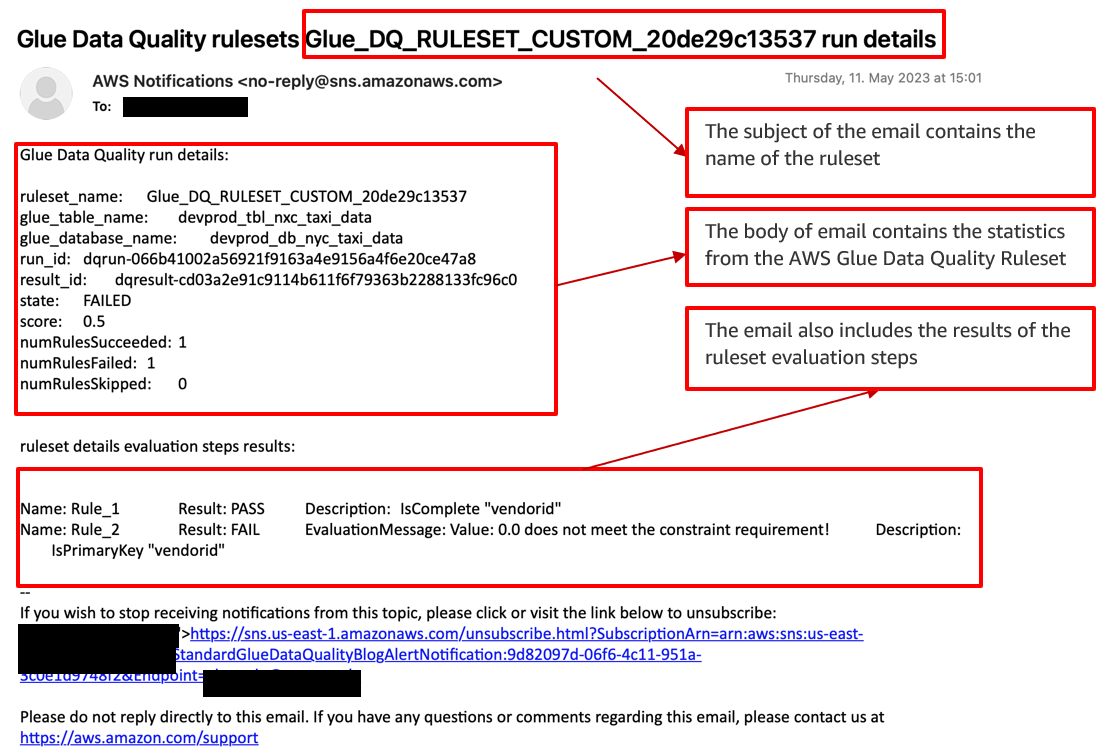
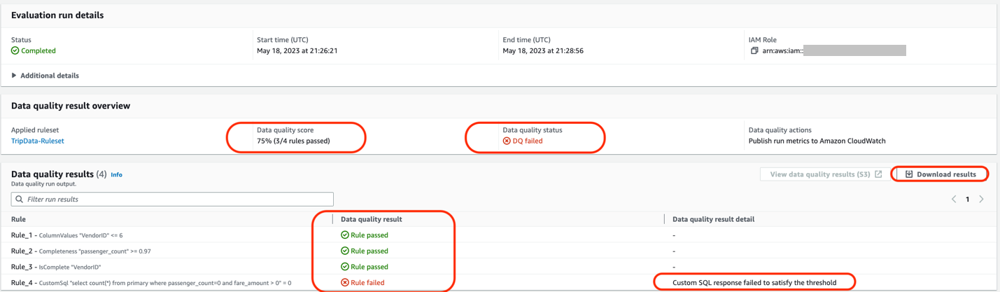
The Step Functions state machine has run AWS the Glue Data Quality evaluation. Now EventBridge matches the pattern Data Quality Evaluations Results Available and triggers the Lambda function. The Lambda function writes customized AWS Glue Data Quality metrics results to the S3 bucket and sends an email notification via Amazon SNS.

The following sample email provides operational metrics for the AWS Glue Data Quality ruleset evaluation. It provides details about the ruleset name, the number of rules passed or failed, and the score. This helps you visualize the results of each rule along with the evaluation message if a rule fails.

You have the flexibility to choose between two run modes for the Step Functions workflow:

  • The first option is on-demand mode, where you manually trigger the Step Functions workflow whenever you want to initiate the AWS Glue Data Quality evaluation.
  • Alternatively, you can schedule the entire Step Functions workflow using EventBridge. With EventBridge, you can define a schedule or specific triggers to automatically initiate the workflow at predetermined intervals or in response to specific events. This automated approach reduces the need for manual intervention and streamlines the data quality evaluation process. For more details, refer to Schedule a Serverless Workflow.

Clean up

To avoid incurring future charges and to clean up unused roles and policies, delete the resources you created:

  1. On the AWS CloudFormation console, choose Stacks in the navigation pane.
  2. Select your stack and delete it.

If you’re continuing to Part 5 in this series, you can skip this step.

Conclusion

In this post, we discussed three key steps that organizations can take to optimize data quality and reliability on AWS:

  • Create a CloudFormation template to ensure consistency and reproducibility in deploying AWS resources.
  • Integrate AWS Glue Data Quality ruleset evaluation and Lambda to automatically evaluate data quality and receive event-driven alerts and email notifications via Amazon SNS. This significantly enhances the accuracy and reliability of your data.
  • Use Step Functions to orchestrate AWS Glue Data Quality ruleset actions. You can create and evaluate custom and recommended rulesets, optimizing data quality and accuracy.

These steps form a comprehensive approach to data quality and reliability on AWS, helping organizations maintain high standards and achieve their goals.

To dive into the AWS Glue Data Quality APIs, refer to Data Quality APIs. To learn more about AWS Glue Data Quality, check out the AWS Glue Data Quality Developer Guide.

If you require any assistance in constructing this pipeline within the AWS Lake Formation environment or if you have any inquiries regarding this post, please inform us in the comments section or initiate a new thread on the Lake Formation forum.


About the authors

Avik Bhattacharjee is a Senior Partner Solution Architect at AWS. He works with customers to build IT strategy, making digital transformation through the cloud more accessible, focusing on big data and analytics and AI/ML.

Amit Kumar Panda is a Data Architect at AWS Professional Services who is passionate about helping customers build scalable data analytics solutions to enable making critical business decisions.

Neel Patel is a software engineer working within GlueML. He has contributed to the AWS Glue Data Quality feature and hopes it will expand the repertoire for all AWS CloudFormation users along with displaying the power and usability of AWS Glue as a whole.

Edward Cho is a Software Development Engineer at AWS Glue. He has contributed to the AWS Glue Data Quality feature as well as the underlying open-source project Deequ.

Set up advanced rules to validate quality of multiple datasets with AWS Glue Data Quality

Post Syndicated from Navnit Shukla original https://aws.amazon.com/blogs/big-data/set-up-advanced-rules-to-validate-quality-of-multiple-datasets-with-aws-glue-data-quality/

Data is the lifeblood of modern businesses. In today’s data-driven world, companies rely on data to make informed decisions, gain a competitive edge, and provide exceptional customer experiences. However, not all data is created equal. Poor-quality data can lead to incorrect insights, bad decisions, and lost opportunities.

AWS Glue Data Quality measures and monitors the quality of your dataset. It supports both data quality at rest and data quality in AWS Glue extract, transform, and load (ETL) pipelines. Data quality at rest focuses on validating the data stored in data lakes, databases, or data warehouses. It ensures that the data meets specific quality standards before it is consumed. Data quality in ETL pipelines, on the other hand, ensures the quality of data as it moves through the ETL process. It helps identify data quality issues during the ETL pipeline, allowing for early detection and correction of problems and prevents the failure of the data pipeline because of data quality issues.

This is Part 3 of a five-post series on AWS Glue Data Quality. In this post, we demonstrate the advanced data quality checks that you can typically perform when bringing data from a database to an Amazon Simple Storage Service (Amazon S3) data lake. Check out the other posts in this series:

Use case overview

Let’s consider an example use case where we have a database named classicmodels that contains retail data for a car dealership. This example database includes sample data for various entities, such as Customers, Products, ProductLines, Orders, OrderDetails, Payments, Employees, and Offices. You can find more details about this example database in MySQL Sample Database.

In this scenario, we assume the role of a data engineer who is responsible for building a data pipeline. The primary objective is to extract data from a relational database, specifically an Amazon RDS for MySQL database, and store it in Amazon S3, which serves as a data lake. After the data is loaded into the data lake, the data engineer is also responsible for performing data quality checks to ensure that the data in the data lake maintains its quality. To achieve this, the data engineer uses the newly launched AWS Glue Data Quality evaluation feature.

The following diagram illustrates the entity relationship model that describes the relationships between different tables. In this post, we use the employees, customers, and products table.

Solution overview

This solution focuses on transferring data from an RDS for MySQL database to Amazon S3 and performing data quality checks using the AWS Glue ETL pipeline and AWS Glue Data Catalog. The workflow involves the following steps:

  1. Data is extracted from the RDS for MySQL database using AWS Glue ETL.
  2. The extracted data is stored in Amazon S3, which serves as the data lake.
  3. The Data Catalog and AWS Glue ETL pipeline are utilized to validate the successful completion of data ingestion by performing data quality checks on the data stored in Amazon S3.

The following diagram illustrates the solution architecture.

To implement the solution, we complete the following steps:

  1. Set up resources with AWS CloudFormation.
  2. Establish a connection to the RDS for MySQL instance from AWS Cloud9.
  3. Run an AWS Glue crawler on the RDS for MySQL database.
  4. Validate the Data Catalog.
  5. Run an AWS Glue ETL job to bring data from Amazon RDS for MySQL to Amazon S3.
  6. Evaluate the advanced data quality rules in the ETL job.
  7. Evaluate the advanced data quality rules in the Data Catalog.

Set up resources with AWS CloudFormation

This post includes a CloudFormation template for a quick setup. You can review and customize it to suit your needs. The template generates the following resources:

  • An RDS for MySQL database instance (source)
  • An S3 bucket for the data lake (destination)
  • An AWS Glue ETL job to bring data from source to destination
  • An AWS Glue crawler to crawl the RDS for MySQL databases and create a centralized Data Catalog
  • AWS Identity and Access Management (IAM) users and policies
  • An AWS Cloud9 environment to connect to the RDS DB instance and create a sample dataset
  • An Amazon VPC, public subnet, two private subnets, internet gateway, NAT gateway, and route tables

To launch the CloudFormation stack, complete the following steps:

  1. Sign in to the AWS CloudFormation console.
  2. Choose Launch Stack:
    BDB-2063-launch-cloudformation-stack
  3. Choose Next.
  4. For DatabaseUserPassword, enter your preferred password.
  5. Choose Next.
  6. Scroll to the end and choose Next.
  7. Select I acknowledge that AWS CloudFormation might create IAM resources with custom names and choose Submit.

This stack can take around 10 minutes to complete, after which you can view the deployed stack on the AWS CloudFormation console.

Establish a connection to the RDS for MySQL instance from AWS Cloud9

To connect to the RDS for MySQL instance, complete the following steps:

  1. On the AWS Cloud9 console, choose Open under Cloud9 IDE for your environment.
  2. Run the following command to the AWS Cloud9 terminal. Provide your values for the MySQL endpoint (located on the CloudFormation stack’s Outputs tab), database user name, and database user password:
    $ mysql --host=<MySQLEndpoint> --user=<DatabaseUserName> password=<password>

  3. Download the SQL file.
  4. On the File menu, choose Upload from Local Files and upload the file to AWS Cloud9.
  5. Run the following SQL commands within the downloaded file:
    MySQL [(none)]> source mysqlsampledatabase.sql

  6. Retrieve a list of tables using the following SQL statement and make sure that eight tables are loaded successfully:
    use classicmodels;
    show tables;

Run an AWS Glue crawler on the RDS for MySQL database

To run your crawler, complete the following steps:

  1. On the AWS Glue console, choose Crawlers under Data Catalog in the navigation pane.
  2. Locate and run the crawler dq-rds-crawler.

The crawler will take a few minutes to crawl all the tables from the classicmodels database.

Validate the AWS Glue Data Catalog

To validate the Data Catalog when the crawler is complete, complete the following steps:

  1. On the AWS Glue console, choose Databases under Data Catalog in the navigation pane.
  2. Choose the mysql_private_classicmodels database.

You will able to see all the RDS tables available under mysql_private_classicmodels.

Run an AWS Glue ETL job to bring data from Amazon RDS for MySQL to Amazon S3

To run your ETL job, complete the following steps:

  1. On the AWS Glue console, choose Visual ETL under ETL jobs in the navigation pane.
  2. Select dq-rds-to-s3 from the job list and choose Run job.

When the job is complete, you will able to see three new tables under mysql_s3_db. It may take a few minutes to complete.

Now let’s dive into evaluating the data quality rules.

Evaluate the advanced data quality rules in the ETL job

In this section, we evaluate the results of different data quality rules.

ReferentialIntegrity

Let’s start with referential integrity. The ReferentialIntegrity data quality ruleset is currently supported in ETL jobs. This feature ensures that the relationships between tables in a database are maintained. It checks if the foreign key relationships between tables are valid and consistent, helping to identify any referential integrity violations.

  1. On the AWS Glue console, choose Visual ETL under ETL jobs in the navigation pane.
  2. In AWS Glue Studio, select Visual with a blank canvas.
  3. Provide a name for your job; for example, RDS ReferentialIntegrity.
  4. Choose the plus sign in the AWS Glue Studio canvas and on the Data tab, choose AWS Glue Data Catalog.
  5. For Name, enter a name for your data source; for example, employees.
  6. For Database, choose mysql_private_classicmodels.
  7. For Table, choose mysql_classicmodels_employees.
  8. Choose the plus sign in the AWS Glue Studio canvas and on the Data tab, choose AWS Glue Data Catalog.
  9. For Name, enter a name for your data source; for example, customers.
  10. For Database, choose mysql_private_classicmodels.
  11. For Table, choose mysql_classicmodels_employees.
  12. Choose the plus sign in the AWS Glue Studio canvas and on the Transform tab, choose Evaluate Data Quality.
  13. For Node parents, choose employees and customers.
  14. For Aliases for referenced data source, select Primary source for employees and for customers, enter the alias customers.

All other datasets are used as references to ensure that the primary dataset has good-quality data.

  1. Search for ReferentialIntegrity under Rule types and choose the plus sign to add an example ReferentialIntegrity rule.
  2. Replace the rule with the following code and keep the remaining options as default:
    Rules = [
        ReferentialIntegrity "employeenumber" "customers.salesRepEmployeeNumber" between 0.6 to 0.7
    ]

  3. Under Data quality action, select Publish results to Amazon CloudWatch and select Fail job without loading target data.
  4. On the Job details tab, choose GlueServiceRole-for-gluedq-blog for IAM role and keep the remaining options as default.
  5. Choose Run and wait for the job to complete.

It will take a few minutes to complete.

  1. When the job is complete, navigate to the Data quality tab and locate the Data quality results section.

You can confirm if the job completed successfully and which data quality rules it passed. In this example, it indicates that 60–70% of EmployeeNumber from the employees table are present in the customers table.

You can identify which records failed the referential integrity using AWS Glue Studio. To learn more, refer to Getting started with AWS Glue Data Quality for ETL Pipelines.

Similarly, if you are checking if all the EmployeeNumber from the employees table are present in the customers table, you can pass the following rule:

Rules = [
    ReferentialIntegrity "employeenumber" "customers.salesRepEmployeeNumber" = 1
]

DatasetMatch

DatasetMatch compares two datasets to identify differences and similarities. You can use it to detect changes between datasets or to find duplicates, missing values, or inconsistencies across datasets.

  1. On the AWS Glue console, choose Visual ETL under ETL jobs in the navigation pane.
  2. In AWS Glue Studio, select Visual with a blank canvas.
  3. Provide a name for your job; for example, RDS DatasetMatch.
  4. Choose the plus sign in the AWS Glue Studio canvas and on the Data tab, choose AWS Glue Data Catalog.
  5. For Name, enter a name for your data source; for example, rds_employees_primary.
  6. For Database, choose mysql_private_classicmodels.
  7. For Table, choose mysql_classicmodels_employees.
  8. Choose the plus sign in the AWS Glue Studio canvas and on the Data tab, choose AWS Glue Data Catalog.
  9. For Name, enter a name for your data source; for example, s3_employees_reference.
  10. For Database, choose mysql_s3_db.
  11. For Table, choose s3_employees.
  12. Choose the plus sign in the AWS Glue Studio canvas and on the Transform tab, choose Evaluate Data Quality.
  13. For Node parents, choose employees and customers.
  14. For Aliases for referenced data source, select Primary source for rds_employees_primary and for s3_employees_reference, enter the alias reference.
  15. Replace the default example rules with the following code and keep the remaining options as default:
    Rules = [
        DatasetMatch "reference" "employeenumber,employeenumber" = 1
    ]

  16. On the Job details tab, choose GlueServiceRole-for-gluedq-blog for IAM role and keep the remaining options as default.
  17. Choose Run and wait for the job to complete.
  18. When the job is complete, navigate to the Data quality tab and locate the Data quality results section.

In this example, it indicates both datasets are identical.

AggregateMatch

AggregateMatch verifies the accuracy of aggregated data. It compares the aggregated values in a dataset against the expected results to identify any discrepancies, such as incorrect sums, averages, counts, or other aggregate calculations. This is a performant option to evaluate if two datasets match at an aggregate level. For this rule, we clone the previous job we created for DatasetMatch.

  1. On the AWS Glue console, choose Visual ETL under ETL jobs in the navigation pane.
  2. Select RDS DatasetMatch and on the Actions menu, choose Clone job.
  3. Change the job name to DQ AggregateMatch.
  4. Change the dataset rds_employees_primary to rds_products_primary and the table to mysql_classicmodels_products.
  5. Change the dataset s3_orders_reference to s3_products_reference and the table to s3_products.
  6. Choose Evaluate Data Quality, and under Node parents, choose rds_products_primary and s3_products_reference.
  7. Replace the rules with the following code:
    AggregateMatch "avg(MSRP)" "avg(reference.MSRP)" = 1

  8. Choose Run and wait for the job to complete.
  9. When the job is complete, navigate to the Data quality tab and locate the Data quality results section.

The results indicate that the avg(msrp) on both datasets is the same.

RowCountMatch

RowCountMatch checks the number of rows in a dataset and compares it to an expected count. It helps identify missing or extra rows in a dataset, ensuring data completeness. For this rule, we edit the job we created earlier for AggregateMatch.

  1. On the AWS Glue console, choose Visual ETL under ETL jobs in the navigation pane.
  2. Select RDS AggregateMatch and on the Actions menu, choose Edit job.
  3. Choose Evaluate Data Quality and choose the plus sign next to RowCountMatch.
  4. Keep the default data quality rules and choose Save:
    RowCountMatch "reference" = 1.0

  5. Choose Run and wait for the job to complete.
  6. When the job is complete, navigate to the Data quality tab and locate the Data quality results section.

It shows that the DQ RowCountMatch rule failed, indicating a mismatch between the row count of the source RDS table and the target S3 table. Further investigation reveals that the ETL job ran four times for the Products table, and the row counts didn’t match.

SchemaMatch

SchemaMatch validates the schema of two datasets matches. It checks if the actual data types match the expected data types and flags any inconsistencies, such as a numeric column containing non-numeric values. For this rule, we edit the job we used for AggregateMatch.

  1. On the AWS Glue console, choose Visual ETL under ETL jobs in the navigation pane.
  2. Select RDS AggregateMatch and on the Actions menu, choose Edit job.
  3. Choose Evaluate Data Quality and choose the plus sign next to RowCountMatch.
  4. Update the default rules with the following code and save the job:
    SchemaMatch "reference" = 1.0

  5. Choose Run and wait for the job to complete.
  6. When the job is complete, navigate to the Data quality tab and locate the Data quality results section.

It should show a successful completion with a Rule passed status, indicating that the schemas of both datasets are identical.

Evaluate the advanced data quality rules in the Data Catalog

The AWS Glue Data Catalog also supports advanced data quality rules. For this post, we show one example of an aggregate match between Amazon S3 and Amazon RDS.

  1. On the AWS Glue console, choose Databases in the navigation pane.
  2. Choose the mysql_private_classicmodels database to view the three tables created under it.
  3. Choose the mysql_classicmodels_products table.
  4. On the Data quality tab, choose Create data quality rules.
  5. Search for AggregateMatch and choose the plus sign to view the default example rule.
  6. Add the following rules:
    Rules = [
        AggregateMatch "avg(msrp)" "avg(mysql_s3_db.s3_products.msrp)" >= 0.9,
        ReferentialIntegrity "productname,productcode" "mysql_s3_db.s3_products.{productname,productcode}" = 1
        ]

reference is the alias of the secondary dataset defined in the AWS Glue ETL job. For the Data Catalog, you can use <database_name>.<table_name>.<column_name> to reference secondary datasets.

  1. Choose Save ruleset and provide the name production_catalog_dq_check.
  2. Choose GlueServiceRole-for-gluedq-blog for IAM role and keep the remaining options as default.
  3. Choose Run and wait for the data quality check to complete.

When the job is complete, you can confirm that both data quality checks passed.

With these advanced data quality features of AWS Glue Data Quality, you can enhance the reliability, accuracy, and consistency of your data, leading to better insights and decision-making.

Clean up

To clean up your resources, complete the following steps:

  1. Delete the AWS Glue job.
  2. Delete the CloudFormation stack.

Conclusion

Data quality refers to the accuracy, completeness, consistency, timeliness, and validity of the information being collected, processed, and analyzed. High-quality data is essential for businesses to make informed decisions, gain valuable insights, and maintain their competitive advantage. As data complexity increases, advanced rules are critical to handle complex data quality challenges. The rules we demonstrated in this post can help you manage the quality of data that lives in disparate data sources, providing you the capabilities to reconcile them. Try them out and provide your feedback on what other use cases you need to solve!


About the authors

Navnit Shukla is AWS Specialist Solutions Architect in Analytics. He is passionate about helping customers uncover insights from their data. He builds solutions to help organizations make data-driven decisions.

Rahul Sharma is a Software Development Engineer at AWS Glue. He focuses on building distributed systems to support features in AWS Glue. He has a passion for helping customers build data management solutions on the AWS Cloud.

Edward Cho is a Software Development Engineer at AWS Glue. He has contributed to the AWS Glue Data Quality feature as well as the underlying open-source project Deequ.

Shriya Vanvari is a Software Developer Engineer in AWS Glue. She is passionate about learning how to build efficient and scalable systems to provide better experience for customers. Outside of work, she enjoys reading and chasing sunsets.

Getting started with AWS Glue Data Quality from the AWS Glue Data Catalog

Post Syndicated from Stuti Deshpande original https://aws.amazon.com/blogs/big-data/getting-started-with-aws-glue-data-quality-from-the-aws-glue-data-catalog/

AWS Glue is a serverless data integration service that makes it simple to discover, prepare, and combine data for analytics, machine learning (ML), and application development. You can use AWS Glue to create, run, and monitor data integration and ETL (extract, transform, and load) pipelines and catalog your assets across multiple data stores.

Hundreds of thousands of customers use data lakes for analytics and ML to make data-driven business decisions. Data consumers lose trust in data if it isn’t accurate and recent, making data quality essential for undertaking optimal and correct decisions.

Evaluation of the accuracy and freshness of data is a common task for engineers. Currently, various tools are available to evaluate data quality. However, these tools often require manual processes of data discovery and expertise in data engineering and coding.

AWS Glue Data Quality is a new feature of AWS Glue that measures and monitors the data quality of Amazon Simple Storage Service (Amazon S3)-based data lakes, data warehouses, and other data repositories. AWS Glue Data Quality can be accessed in the AWS Glue Data Catalog and in AWS Glue ETL jobs.

This is Part 1 of a five-part series of posts to explain how AWS Glue Data Quality works. Check out the next posts in the series:

In this post, we explore using the AWS Glue Data Quality feature by generating data quality recommendations and running data quality evaluations on your table in the Data Catalog. Then we demonstrate how to analyze your AWS Glue Data Quality run results through Amazon Athena.

Solution overview

We guide you through the following steps:

  1. Provision resources with AWS CloudFormation.
  2. Explore the generated recommendation rulesets and define rulesets to evaluate your table in the Data Catalog.
  3. Review the AWS Glue Data Quality recommendations.
  4. Analyze your AWS Glue Data Quality evaluation results with Athena.
  5. Operationalize the solution by setting up alerts and notifications using integration with Amazon EventBridge and Amazon Simple Notification Service (Amazon SNS).

For this post, we use the NYC Taxi dataset yellow_tripdata_2022-01.parquet.

Set up resources with AWS CloudFormation

The provided CloudFormation template creates the following resources for you:

  • The AWS Identity and Access Management (IAM) role required to run AWS Glue Data Quality evaluations
  • An S3 bucket to store the NYC Taxi dataset
  • An S3 bucket to store and analyze the results of AWS Glue Data Quality evaluations
  • An AWS Glue database and table created from the NYC Taxi dataset

Launch your CloudFormation stack

To create your resources for this use case, complete the following steps:

  1. Launch your CloudFormation stack in us-east-1:
    BDB-2063-launch-cloudformation-stack
  2. Under Parameters:
    • For Stack name, proceed with the default value myDQStack.
    • For DataQualityDatabase, proceed with the default value data_quality_catalog.
    • For DataQualityS3BucketName, provide a bucket name of your choice.
    • For DataQualityTable, proceed with the default value data_quality_tripdata_table

  3. Select I acknowledge that AWS CloudFormation might create IAM resources with custom names.
  4. Choose Create stack.

After the stack is successfully created, you can see all the resources created on the Resources tab.

  1. Navigate to the S3 bucket created by the stack and upload the yellow_tripdata_2022-01.parquet file.

Explore recommendation rulesets and define rulesets to evaluate your table

In this section, we generate data quality rule recommendations from AWS Glue Data Quality. We use these recommendations to run a data quality task against our dataset to obtain an analysis of our data.

Complete the following steps:

  1. On the AWS Glue console, under Data Catalog in the navigation pane, choose Tables.
  2. Choose the data_quality_tripdata_table table created via the CloudFormation stack.
  3. Choose the Data quality tab.

In this section, you will find a video to get you started with AWS Glue Data Quality. It also lists features, pricing, and documentation.

  1. Choose Create data quality rules.

This is the ruleset console. You will find a Request data quality rule recommendations banner at the top. AWS Glue will scan your data and automatically generate rule recommendations.

  1. Choose Recommend rules.
  2. For IAM role, choose the IAM role created as part of the Cloud Formation template (GlueDataQualityBlogRole).
  3. Optionally, you can filter your data before reading on column values. This feature is available for Amazon S3-based data sources.
  4. For Requested number of workers, allocate the number of workers to run the recommendation task. For this post, we use the default value of 5.
  5. For Task timeout, set the runtime for this task. For this post, we use the default of 120 minutes.
  6. Choose Recommend rules.

The recommendation task will start instantly, and you will observe the status on the top changes to Starting.

Next, we add some of these recommended rules into our ruleset.

  1. When you see the recommendation run as Completed, choose Insert rule recommendations to select the rules that are recommended for you.

Make sure to place the cursor inside the brackets Rules = [ ].

  1. Select the following rules:
    • ColumnValues “VendorID” <=6
    • Completeness “passenger_count”>=0.97
  2. Choose Add selected rules.

You can see that these rules were automatically added to the ruleset.

Understanding AWS Glue Data Quality recommendations

AWS Glue Data Quality recommendations are suggestions generated by the AWS Glue Data Quality service and are based on the shape of your data. These recommendations automatically take into account aspects like row counts, mean, standard deviation, and so on, and generate a set of rules for you to use as a starting point.

The dataset used here was the NYC Taxi dataset. Based on this, the columns in this dataset, and the values of those columns, AWS Glue Data Quality recommends a set of rules. In total, the recommendation service automatically took into consideration all the columns of the dataset, and recommended 55 rules.

Some of these rules are:

  • ColumnValues “VendorID” <=6 – The ColumnValues rule type checks the percentage of complete (non-null) values in a column against a given expression. This rule resolves to true if the rule type response is less than or equal to value 6.
  • Completeness “passenger_count”>=0.97 – The Completeness rule type checks the percentage of complete (non-null) values in a column against a given expression. In this case, the rule checks if more than 97% of the values in a column are complete.

In addition to adding auto-generated recommendation rules, we manually add some rules to the ruleset. AWS Glue Data Quality provides some out-of-the-box rule types to choose from. For this post, we manually add the IsComplete rule for VendorID.

  1. In the left pane, on the Rule types tab, search IsComplete rule type and choose the plus sign next to IsComplete to add this rule.
  2. For the value within the quotation marks, enter VendorID.

Conversely, you could navigate to the Schema tab and add IsComplete to VendorID.

  1. Choose Save ruleset.

Next, we add a CustomSQL rule by selecting the rule type CustomSql, that validates that there are no fares charged for a trip if there are no passengers. This is to identify if there are any fraudulent transactions for fare_amount > 0 where passenger_count = 0. The rule is:

CustomSql "select count(*) from primary where passenger_count=0 and fare_amount > 0" = 0

There are two ways to provide the table name:

  • Either you can use the keyword “primary” for the table under consideration
  • You can use the full path such as database_name.table_name
  1. On the Rule types tab, choose the plus sign next to CustomSQL and enter the SQL statement.

The final ruleset looks like the following screenshot.

  1. Choose Save ruleset.
  2. For Ruleset name, enter a name.
  3. Choose Save ruleset.
  4. On the ruleset page, choose Run.
  5. For IAM role¸ choose GlueDataQualityBlogRole.
  6. Select Publish run metrics to Amazon CloudWatch.
  7. For Data quality result location, enter the S3 bucket location for the data quality results which is already created for you as part of Cloud Formation template (for this post, data-quality-tripdata-results).
  8. For Run frequency, choose On demand.
  9. Expand Additional configurations.
  10. For Requested number of workers, enter 5.
  11. Leave the remaining fields as is and choose Run.

The status changes to Starting.

  1. When it’s complete, choose the ruleset and choose Run history.
  2. Choose the run ID to find more about the run details.

Under Data quality result, you will also observe the result shows as DQ passed or DQ failed.

In the Evaluation run details section, you will find all the details about the data quality task run and rules that passed or failed. You can either view these results by navigating to the S3 bucket or downloading the results. Observe that the data quality task failed because one of the rules failed.

For the first section, AWS Glue Data Quality suggested 51 rules, based on the column values and the data within our NYC Taxi dataset. We selected a few rules out of the 51 rules into a ruleset and ran an AWS Glue Data Quality evaluation task using our ruleset against our dataset. In our results, we see the status of each rule within the run details of the data quality task.

You can also utilize the AWS Glue Data Quality APIs to carry out these steps.

Analyze your AWS Glue Data Quality evaluation results with Athena

If you have multiple AWS Glue Data Quality evaluation results against a dataset, you might want to track the trends of the dataset’s quality over a period of time. To achieve this, we can export our AWS Glue Data Quality evaluation results to Amazon S3, and use Athena to run analytical queries against the exported results. You could further use the results in Amazon QuickSight to build dashboards to have a graphical representation of your data quality trends

In Part 3 of this series, we show the steps needed to start tracking data on your dataset’s quality.

For our data quality runs that we set up in the previous sections, we set the Data quality results location parameter to the bucket location specified by the CloudFormation stack. After each successful run, you should see a Parquet format file that contains a single JSONL file being exported to your selected S3 location, corresponding to that particular run.

Complete the following steps to analyze the data:

  1. Navigate to Amazon Athena and on the console, navigate to Query Editor.
  2. Run the following CREATE TABLE statement (replace the <my_table_name> with a relevant value of your choice and <GlueDataQualityResultsS3Bucket_from_cfn> with the S3 bucket name to store data-quality results; the bucket name will have trailing keyword results, for example <given-name-results>. For this post, it is data-quality-tripdata-results.
    CREATE EXTERNAL TABLE `<my_table_name>`(
    `catalogid` string,
    `databasename` string,
    `tablename` string,
    `dqrunid` string,
    `evaluationstartedon` timestamp,
    `evaluationcompletedon` timestamp,
    `rule` string,
    `outcome` string,
    `failurereason` string,
    `evaluatedmetrics` string)
    PARTITIONED BY (
    `year` string,
    `month` string,
    `day` string)
    ROW FORMAT SERDE
    'org.openx.data.jsonserde.JsonSerDe'
    WITH SERDEPROPERTIES (
    'paths'='catalogId,databaseName,dqRunId,evaluatedMetrics,evaluationCompletedOn,evaluationStartedOn,failureReason,outcome,rule,tableName')
    STORED AS INPUTFORMAT
    'org.apache.hadoop.mapred.TextInputFormat'
    OUTPUTFORMAT
    'org.apache.hadoop.hive.ql.io.HiveIgnoreKeyTextOutputFormat'
    LOCATION
    's3://<GlueDataQualityResultsS3Bucket_from_cfn>/'
    TBLPROPERTIES (
    'classification'='json',
    'compressionType'='none',
    'typeOfData'='file')
    MSCK REPAIR TABLE `<my_table_name>`

After you create the table, you should be able to run queries to analyze your data quality results.

For example, consider the following query that shows the passed AWS Glue Data Quality evaluations against the table data_quality_tripdata_table within a certain time window. You can select the datetime values from the data quality results table (that you created above) <my_table_name> from the columns evaluationcompletedon to specify values for parse_datetime() within a certain duration in the following query:

SELECT * from `<my_table_name>`
WHERE "outcome" = 'Passed'
AND "tablename" = `data_quality_tripdata_table`
AND "evaluationcompletedon" between
parse_datetime('2023-05-12 00:00:00:000', 'yyyy-MM-dd HH:mm:ss:SSS') AND parse_datetime('2023-05-12 21:16:21:804', 'yyyy-MM-dd HH:mm:ss:SSS');

The output of the preceding query shows us details about all the runs with “outcome” = ‘Passed’ that ran against the NYC Taxi dataset table (“tablename” = ‘data_quality_tripdata_table’). The output also provides details about the rules passed and evaluated metrics.

As you can see, we are able to get detailed information about our AWS Glue Data Quality evaluations via the results uploaded to Amazon S3 and perform more detailed analysis.

Set up alerts and notifications using EventBridge and Amazon SNS

Alerts and notifications are important for data quality to enable timely and effective responses to data quality issues that arise in the dataset. By setting up alerts and notifications, you can proactively monitor the data quality and be alerted as soon as any data quality issues are detected. This reduces the risk of making decisions based on incorrect information.

AWS Glue Data Quality also offers integration with EventBridge for alerting and notification by triggering an AWS Lambda function that sends a customized SNS notification when the AWS Glue Data Quality ruleset evaluation is complete. Now you can receive event-driven alerts and email notifications via Amazon SNS. This integration significantly enhances the accuracy and reliability of data.

Clean up

To clean up your resources, complete the following steps:

  1. On the Athena console, delete the table created for data quality analysis.
  2. On the CloudWatch console, delete the alarms created.
  3. If you deployed the sample CloudFormation stack, delete the stack via the AWS CloudFormation console. You will need to empty the S3 bucket before you delete the bucket.
  4. If you enabled your AWS Glue Data Quality runs to output to Amazon S3, empty those buckets as well.

Conclusion

In this post, we talked about the ease and speed of incorporating data quality rules using AWS Glue Data Quality into your Data Catalog tables. We also talked about how to run recommendations and evaluate data quality against your tables. We then discussed analyzing the data quality results via Athena, and discussed integrations with EventBridge and Amazon SNS for alerts and notifications to get notified for data quality issues.

To dive into the AWS Glue Data Quality APIs, refer to Data Quality API documentation. To learn more about AWS Glue Data Quality, check out AWS Glue Data Quality.


About the authors

Stuti Deshpande is an Analytics Specialist Solutions Architect at AWS. She works with customers around the globe, providing them strategic and architectural guidance on implementing analytics solutions using AWS. She has extensive experience in Big Data, ETL, and Analytics. In her free time, Stuti likes to travel, learn new dance forms, and enjoy quality time with family and friends.

Aniket Jiddigoudar is a Big Data Architect on the AWS Glue team. He works with customers to help improve their big data workloads. In his spare time, he enjoys trying out new food, playing video games, and kickboxing.

Joseph Barlan is a Frontend Engineer at AWS Glue. He has over 5 years of experience helping teams build reusable UI components and is passionate about frontend design systems. In his spare time, he enjoys pencil drawing and binge watching tv shows.

Jesus Max Hernandez is a Software Development Engineer at AWS Glue. He joined the team in August after graduating from The University of Texas at El Paso. Outside of work, you can find him practicing guitar or playing softball in Central Park.

Divya Gaitonde

is a UX designer at AWS Glue. She has over 8 years of experience driving impact through data-driven products and seamless experiences. Outside of work, you can find her catching up on reading or people watching at a museum.

Deep dive on Amazon MSK tiered storage

Post Syndicated from Nagarjuna Koduru original https://aws.amazon.com/blogs/big-data/deep-dive-on-amazon-msk-tiered-storage/

In the first post of the series, we described some core concepts of Apache Kafka cluster sizing, the best practices for optimizing the performance, and the cost of your Kafka workload.

This post explains how the underlying infrastructure affects Kafka performance when you use Amazon Managed Streaming for Apache Kafka (Amazon MSK) tiered storage. We delve deep into the core components of Amazon MSK tiered storage and address questions such as: How does read and write work in a tiered storage-enabled cluster?

In the subsequent post, we’ll discuss the latency impact, recommended metrics to monitor, and conclude with guidance on key considerations in a production tiered storage-enabled cluster.

How Amazon MSK tiered storage works

To understand the internal architecture of Amazon MSK tiered storage, let’s first discuss some fundamentals of Kafka topics, partitions, and how read and write works.

A logical stream of data in Kafka is referred to as a topic. A topic is broken down into partitions, which are physical entities used to distribute load across multiple server instances (brokers) that serve reads and writes.

A partition––also designated as topic-partition as it’s relative to a given topic––can be replicated, which means there are several copies of the data in the group of brokers forming a cluster. Each copy is called a replica or a log. One of these replicas, called the leader, serves as the reference. It’s where the ingress traffic is accepted for the topic-partition.

A log is an append-only sequence of log segments. Log segments contain Kafka data records, which are added to the end of the log or the active segment.

Log segments are stored as regular files. On the file system, Kafka identifies the file of a log segment by putting the offset of the first data record it contains in its file name. The offset of a record is simply a monotonic index assigned to a record by Kafka when it’s appended to the log. The segment files of a log are stored in a directory dedicated to the associated topic-partition.

When Kafka reads data from an arbitrary offset, it first looks up the segment that contains that offset from the segment file name, then the specific record location inside that file using an offset index. Offset indexes are materialized on a dedicated file stored with segment files in the topic-partition directory. There is also timeindex to seek by timestamp.

For every partition, Kafka also stores a journal of leadership changes in a file called leader-epoch-checkpoint. This file contains mapping of leader epoch to startOffset of the epoch. Whenever a new leader is elected for a partition by the Kafka controller, this data is updated and propagated to all brokers. A leader epoch is a 32-bit, monotonically increasing number representing continuous period of leadership of a single partition. It’s marked on all the Kafka records. The following code is the local storage layout of topic cars and partition 0 containing two segments (0, 35):

$ ls /kafka-cluster/broker-1/data/cars-0/

00000000000000000000.log
00000000000000000000.index
00000000000000000000.timeindex
00000000000000000035.log
00000000000000000035.index
00000000000000000035.timeindex
leader-epoch-checkpoint

Kafka manages the lifecycle of these segment files. It creates a new one when a new segment needs to be created, for instance, if the current segment reaches its configured max size. It deletes one when the target retention period of the data it contains is reached, or the total maximal size of the log is reached. Data is deleted from the tail of the logs and corresponds to the oldest data of the append-only log of the topic-partition.

KIP-405 or tiered storage in Apache Kafka

The ability to tier data, in other words, transfer data (log, index, timeindex, and leader-epoch-checkpoint) from a local file system to another storage system based on time and size-based retention policies, is a feature built in Apache Kafka as part of KIP-405.

The KIP-405 isn’t in official Kafka version yet. Amazon MSK internally implemented tiered storage functionality on top of official Kafka version 2.8.2. Amazon MSK exposes this functionality on AWS specific 2.8.2.tiered Kafka version. With this feature, you can separate retention settings for local and remote retention. Data in the local tier is retained until the data gets copied to the remote tier even after the local retention expires. Data in the remote tier is retained until the remote retention expires. KIP-405 proposes a pluggable architecture allowing you to plugin custom remote storage and metadata storage backends. The following diagram illustrates the broker three key components.

The components are as follows:

  • RemoteLogManager (RLM) – A new component corresponding to LogManager for the local tier. It delegates copy, fetch, and delete of completed and non-active partition segments to a pluggable RemoteStorageManager implementation and maintains respective remote log segment metadata through pluggable RemoteLogMetadataManager implementation.
  • RemoteStorageManager (RSM) – A pluggable interface that provides the lifecycle of remote log segments.
  • RemoteLogMetadataManager (RLMM) – A pluggable interface that provides the lifecycle of metadata about remote log segments.

How data is moved to the remote tier for a tiered storage-enabled topic

In a tiered storage-enabled topic, each completed segment for a topic-partition triggers the leader of the partition to copy the data to the remote storage tier. The completed log segment is removed from the local disks when Amazon MSK finishes moving that log segment to the remote tier and after it meets the local retention policy. This frees up local storage space.

Let’s consider a hypothetical scenario: you have a topic with one partition. Prior to enabling tiered storage for this topic, there are three log segments. One of the segments is active and receiving data, and the other two segments are complete.

After you enable tiered storage for this topic with two days of local retention and five days of overall retention, Amazon MSK copies log segment 1 and 2 to tiered storage. Amazon MSK also retains the primary storage copy of segments 1 and 2. The active segment 3 isn’t eligible to copy over to tiered storage yet. In this timeline, none of the retention settings are applied yet for any of the messages in segment 1 and segment 2.

After 2 days, the primary retention settings take effect for the segment 1 and segment 2 that Amazon MSK copied to the tiered storage. Segments 1 and 2 now expire from the local storage. Active segment 3 is neither eligible for expiration nor eligible to copy over to tiered storage yet because it’s an active segment.

After 5 days, overall retention settings take effect, and Amazon MSK clears log segments 1 and 2 from tiered storage. Segment 3 is neither eligible for expiration nor eligible to copy over to tiered storage yet because it’s active.

That’s how the data lifecycle works on a tiered storage-enabled cluster.

Amazon MSK immediately starts moving data to tiered storage as soon as a segment is closed. The local disks are freed up when Amazon MSK finishes moving that log segment to remote tier and after it meets the local retention policy.

How read works in a tiered storage-enabled topic

For any read request, ReplicaManager tries to process the request by sending it to ReadFromLocalLog. And if the process returns offset out of range exception, it delegates the read call to RemoteLogManager to read from tiered storage. On the read path, the RemoteStorageManager starts fetching the data in chunks from remote storage, which means that for the first few bytes, your consumer experiences higher latency, but as the system starts buffering the segment locally, your consumer experiences latency similar to reading from local storage. One of the advantages of this approach is that the data is served instantly from the local buffer if there are multiple consumers reading from the same segment.

If your consumer is configured to read from the closest replica, there might be a possibility that the consumer from a different consumer group reads the same remote segment using a different broker. In that case, they experience the same latency behavior we described previously.

Conclusion

In this post, we discussed the core components of the Amazon MSK tiered storage feature and explained how the data lifecycle works in a cluster enabled with tiered storage. Stay tuned for our upcoming post, in which we delve into the best practices for sizing and running a tiered storage-enabled cluster in production.

We would love to hear how you’re building your real-time data streaming applications today. If you’re just getting started with Amazon MSK tiered storage, we recommend getting hands-on with the guidelines available in the tiered storage documentation.

If you have any questions or feedback, please leave them in the comments section.


About the authors

Nagarjuna Koduru is a Principal Engineer in AWS, currently working for AWS Managed Streaming For Kafka (MSK). He led the teams that built MSK Serverless and MSK Tiered storage products. He previously led the team in Amazon JustWalkOut (JWO) that is responsible for realtime tracking of shopper locations in the store. He played pivotal role in scaling the stateful stream processing infrastructure to support larger store formats and reducing the overall cost of the system. He has keen interest in stream processing, messaging and distributed storage infrastructure.

Masudur Rahaman Sayem is a Streaming Data Architect at AWS. He works with AWS customers globally to design and build data streaming architectures to solve real-world business problems. He specializes in optimizing solutions that use streaming data services and NoSQL. Sayem is very passionate about distributed computing.

How SumUp made digital analytics more accessible using AWS Glue

Post Syndicated from Mira Daniels original https://aws.amazon.com/blogs/big-data/how-sumup-made-digital-analytics-more-accessible-using-aws-glue/

This is a guest blog post by Mira Daniels and Sean Whitfield from SumUp.

SumUp is a leading global financial technology company driven by the purpose of leveling the playing field for small businesses. Founded in 2012, SumUp is the financial partner for more than 4 million small merchants in over 35 markets worldwide, helping them start, run and grow their business. Through its Super App, SumUp provides merchants with a free business account and card, an online store, and an invoicing solution – as well as in-person and remote payments seamlessly integrated with SumUp’s card terminals and point-of-sale registers. For more information, please visit sumup.co.uk.

As most organizations, that have turned to Google Analytics (GA) as a digital analytics solution, mature they discover a more pressing need to integrate this data silo with the rest of their organization’s data to enable better analytics and resulting product development and fraud detection. Unless, of course, the rest of their data also resides in the Google Cloud. In this post we showcase how we used AWS Glue to move siloed digital analytics data, with inconsistent arrival times, to AWS S3 (our Data Lake) and our central data warehouse (DWH), Snowflake. AWS Glue gave us a cost-efficient option to migrate the data and we further optimized storage cost by pruning cold data. What was essential to the solution development was a good understanding of the nature of the data, the source of it (export from GA) as well as the form and scope of the data useful to the data consumers.

Business context

At SumUp we use GA and Firebase as our digital analytics solutions and AWS as our main Cloud Provider. In order to mature our data marts, it became clear that we needed to provide Analysts and other data consumers with all tracked digital analytics data in our DWH as they depend on it for analyses, reporting, campaign evaluation, product development and A/B testing. We further use the Digital Analytics data for our reverse ETL pipelines that ingest merchant behavior data back into the Ad tools. As the SumUp merchants user journey only starts onsite (with a Sign up or product purchase), but extends to offline card reader transactions or usage of our products from within our app and web dashboard, it is important to combine Digital Analytics data with other (backend) data sources in our Data Lake or DWH. The Data Science teams also use this data for churn prediction and CLTV modeling.

Given that the only source to access all raw data is by exporting it to BigQuery (first), data accessibility becomes challenging if BigQuery isn’t your DWH solution. What we needed was a data pipeline from BigQuery to our Data Lake and the DWH. The pipeline further needed to run based on the trigger of new data arriving in BigQuery and could not run on a simple schedule as data would not arrive at the same time consistently.

We experimented with some no-code tools that allowed for the direct export of Google Analytics data (not available for Firebase) from BigQuery directly to Snowflake, but due to our growing data volume, this wasn’t financially scalable. Other no-code tools, even if they can move data to S3, did not meet our technical requirements. The solutions we experimented with did not give us the flexibility to monitor and scale resources per pipeline run and optimize the pipeline ourselves.

We had a solid business case to build our own internal digital analytics pipeline to not only reduce spending on our existing outsourced Google Analytics pipeline (that moved from BigQuery to Snowflake directly), but also to make GA and Firebase data available in both the Data Lake and DWH.

Technical challenges

Data source specifics: The data in BigQuery is the export of GA 360 data and Firebase Analytics data. It consists of full-day and intraday tables. BigQuery uses a columnar storage format that can efficiently query semi-structured data, in the case of GA and Firebase data as arrays of structs.

Full-day: Daily tables that do not change retroactively for GA data, but for Firebase data

Intraday: Until the daily tables (full-day are created the intraday tables are populated with new and corrected records.

Update interval: intraday is refreshed and overwritten at least 3x a day. When the full-day table is created, the intraday table from that day is deleted.

Since we started exporting GA tracking data to BigQuery in 2015 the amount of data tracked and stored has grown 70x (logical bytes) and is >3TB in total. Our solution needs not only be able to ingest new data but also backfill historical data from the last 7 years. Firebase data has been exported to BigQuery since 2019 and grew 10x in size (logical bytes) over time.

Our major challenge with ingesting Firebase data to the DWH was the combination of its size (historically >35TB) with the arrival of late data upstream. Since BigQuery processes hits with timestamps up to 72 hours earlier for Firebase data, historical data must be updated for each daily run of the pipeline for the last 3 days. Consequently, this greatly increases compute and storage resources required for the pipeline.

The intraday source data usually arrives every 2-4 hours so real-time downstream pipelines are currently not needed with our GA and Firebase data export (into BigQuery) setup.

Querying the dataset (containing nested and repeated fields) in Snowflake presented an accessibility problem for our users, as it required unfriendly verbose query syntax and greatly strained our compute resources. We used AWS Glue to run a UDF to transform this nested data into a Snowflake object (key-value) data structure that is both more user friendly and requires less compute resources to access.

Regarding version control of the Glue script, our team wanted to contain all of the pipeline logic in the same repository for simplicity and ease of local development. Since we used MWAA for orchestrating our platform pipelines, we wanted our DAG code to be close to the Glue Script. This required us to add an initial first step in our pipeline to push the script to the respective bucket that AWS Glue is synced with.

Our ELT design pattern required that we overwrite/update data stored in S3 before loading it into snowflake which required us to use a Spark DF.

In order to save on Snowflake storage costs, we decided to only keep hot data in a materialised table and have access to colder historical data through external tables.

Solution overview

We chose AWS Glue for the first step in the pipeline (moving data to S3) as it nicely integrates into our serverless AWS infrastructure and Pyspark makes it very flexible to script transformation steps and add partitions to the data storage in S3. It already provided a connector to BigQuery that was easy to configure and the complete Glue job was nicely abstracting the underlying system infrastructure.

We used the existing Google BigQuery Connector for Glue following parts of this blog post.

Ingestion

The code for the ingestion pipeline was set up in a way that it is easily extendable and reusable by splitting jobs/tasks in different methods and classes building a framework for all (future) ingestions from BigQuery to Snowflake.

Initialise Glue Job: Firstly, we push the glue script to S3 as the boto3 client expects it to be there for job execution. We then check if the glue job already exists. If it doesn’t exist, it’s created, otherwise it is updated with the most recent job parameters. We made sure to add appropriate tags for cost monitoring.

Pull From Google Cloud Platform: Based on the data source, GA or Firebase, we pick dynamic (or hard coded for backfilling) days to be pulled from the source. We then check if those selected dates exist as sharded tables in BigQuery, in case the data is late we cannot pull it and will wait to try again a few minutes later (using a generous retry schedule). If the dates we chose to be ingested can be found in BigQuery we run the Glue job.

Dump to S3: Some transformation steps are carried out within the Glue job before the data is moved into S3. It is saved in day-partitioned folders and repartitioned into 300-500MB files for better table query performance in Snowflake.

Data Catalog: We also wanted to automate a Glue Crawler to have metadata in a Data Catalog and be able to explore our files in S3 with Athena. With the help of the boto3 library, our pipeline contains a step which runs the crawler at the end of the pipeline. In order to simplify schema evolution, we moved the Data Catalog creation out of the Glue script.

DWH: The solution loading the data to Snowflake consists of tasks that are scheduled to access storage integrations with S3 and materialise the data in Snowflake tables. The jobs are batch jobs, we haven’t tested any streaming solutions as the data arrives batched in BigQuery. After loading new data into Snowflake we use a table pruner function that deletes the respective days that fall outside of the number of days of retention we defined for the table. This way we make sure to provide the data timeframe used by our stakeholders and avoid unnecessary storage costs.

In addition to the materialised tables in Snowflake we use External tables to make more historical data available (at slower query speed), these External tables are refreshed at the end of the data pipeline in Airflow using the Snowflake operator.

Development and Testing: Before the Glue job script was integrated into the task orchestration process and code, we tested the functionality of the job within Glue Studio using the Spark script Editor and Jupyter Notebook. It was great for quick iteration over a new feature. We used boto3 to access AWS infrastructure services and create, update and run the Glue job

Data Quality is ensured on the one hand by deduplicating Firebase events and adding a new hash key within the Glue script and on the other hand by comparing total row counts per day between Snowflake and BigQuery (the comparison is currently done in tableau). We also get alerted if our Airflow pipeline or the Snowflake tasks fail.

In the future we will add Data Quality checks with DBT.

Conclusion

As SumUp expands its product suite through innovation and acquisition, so does its infrastructure. AWS Glue has proven to be a scalable solution to ingest and transform siloed data in different clouds using marketplace connectors and the flexibility provided by pyspark.

What surprised us was how easily Glue can be customized (from no code to highly customised script and execution setup) and fit our volatile source data (size and shape). In the future we can think of further customization of the Glue script in terms of transformation of the data (more useful unnesting) as well as Glue job resource optimization.

The consumers of Digital Analytics data appreciate being able to make use of the full source data schema in both Data Lake and DWH. The transparency around the process being managed by the central Data Platform team facilitates trust and reliance on the data. Through pipeline abstraction, we’re now able to provide data products in high demand to all our data consumers.

The pipeline framework we built can easily be extended if needed as its components were built separately and are only forming the final pipeline during the last step, the orchestration.

What we plan to test and optimize in the future is loading historical data in automated batch jobs which is dependent on both API limits on the source side and compute resource orchestration on Glue’s side (we did not test automated batching in the past and were manually chunking data into jobs for backfilling). Additionally, we will incorporate these pipeline features into our main ingestion framework, which would allow our stakeholders to define digital analytics pipelines themselves in a self-service manner.

If your organization faces similar challenges with digital analytics data silos, we recommend developing a proof of concept to migrate your data to S3 using the Google BigQuery Connector for Glue and this blog post. Experiment with the Glue job settings and PySpark script options to find the best match for the size and latency requirements of your data. For migrating to a DWH like Snowflake, leverage COPY INTO statements as they are a cheaper alternative to Snowpipes for this volume of data. Once you have prototyped, develop a proper well tested solution with Amazon Managed Workflows for Apache Airflow MWAA that includes version control for the infrastructure and the pipeline logic.


About the Authors

Mira Daniels (Data Engineer in Data Platform team), recently moved from Data Analytics to Data Engineering to make quality data more easily accessible for data consumers. She has been focusing on Digital Analytics and marketing data in the past.

Sean Whitfield (Senior Data Engineer in Data Platform team), a data enthusiast with a life science background who pursued his passion for data analysis into the realm of IT. His expertise lies in building robust data engineering and self-service tools. He also has a fervor for sharing his knowledge with others and mentoring aspiring data professionals.

This is Ceti Alpha Five!

Post Syndicated from Owen Holland original https://blog.rapid7.com/2023/06/06/this-is-ceti-alpha-five/

This is Ceti Alpha Five!

Star Trek II: The Wrath of Khan demonstrating the very best and worst of cybersecurity in the 23rd Century

For those new to the Sci-Fi game, Star Trek II: The Wrath of Khan is a 1982 science fiction film based on the 1966-69 television series Star Trek. In the film, Admiral James T. Kirk and the crew of the starship USS Enterprise face off against a genetically engineered tyrant Khan Noonien Singh for control of the Genesis Device (a technology designed to reorganize dead matter into a habitable environment).

It is widely considered the best Star Trek film due to Khan’s capabilities exceeding the Enterprise’s crew and its narrative of no-win scenarios. To celebrate the 41st anniversary of its release, this blog looks at The Wrath of Khan through a cybersecurity lens.

Khan’s Wrath

In the opening scene, Kirk oversees a simulator session of Captain Spock’s trainees. The simulation, called the Kobayashi Maru, is a no-win scenario designed to test the character of Starfleet officers. Like in cybersecurity, a no-win scenario is a situation every commander may face. This is as true today as it was in the ’80s; however, you can certainly even the odds today.

Having a clear cybersecurity mission and vision provides more precise outcomes; however, like Spock was so keen to highlight, we learn by doing, as the journey is a test of character, and maybe that was the lesson of the simulation.

We then learn how Khan seeks to escape from a 15-year exile on an uninhabitable planet and exact revenge on Kirk. Khan is genetically engineered, and his physical strength and intelligence are abnormal. As a result, he is prone to having grand visions and likely has a superiority complex. Unsurprisingly, his own failures and those of his crew reverberate around him, consuming him and giving him a single unstoppable focus.

In a cybersecurity context, Khan represents threat actors slowly descending on you and your organisation. They are driven to succeed, to inflict pain, gain an advantage, and steal technology. Most, like Khan, have a crew, a band of like-minded individuals with a common objective. If Khan, in this example, is the threat actor, the Starfleet represents an organization operating in today’s threat landscape.

Ceti Alpha FAIL!

There’s no other way to describe it; there are simply some forehead-slapping moments regarding basic cybersecurity practices in The Wrath of Khan. For example, the starship Reliant, a science vessel, is on a mission to search for a lifeless planet called Ceti Alpha Five to test the Genesis Device. Two Reliant officers beam down to the planet, which they believe to be uninhabited. Once there, they are captured by Khan as part of his plan to seek revenge against Kirk.

Khan implants the two crew members with indigenous eel larvae that render them susceptible to mind control (Think Insider Threat.) and uses them to capture the starship Reliant. With seemingly no quarantine procedures in place, they return to the Reliant, and quickly beam Khan and his crew aboard.

However, just like a cyber threat actor, Khan doesn’t stop there. He wants more… and since everything has gone unnoticed so far, he can press home his advantage. He learns about the Genesis project the science team supported and quickly realizes that he can use the device as a weapon.

The Hubris of the Defeated

Next, the Enterprise receives a distress call from the space station to which the Reliant is assigned. There are several examples of poor cybersecurity best practices in this scene; so the audience knows an attack is about to happen, but the Enterprise crew are completely unaware. This scenario is similar to the cybersecurity vulnerabilities many modern organisations face without completely understanding their risks.

The Enterprise, still operated by Spock’s trainees, encounters the Reliant en route to the space station. Ignorant of the forthcoming danger, Kirk approaches the Reliant with its shields down; and Khan draws them closer with false communications until they are in striking range.

The junior bridge officer, Commander Saavik, quotes General Order 12: ‘When approaching a vessel with which communications has not been established, all Starfleet vessels are to maintain maximum safety precautions... but she is cut off. Kirk carries on despite having processes for just such a risky encounter AND having just received a distress call from the space station. Failing to follow security guidelines makes Khan’s surprise attack even more powerful.

Going into an unknown encounter with their shields down and with the opposition having sufficient time to plan the attack, the Enterprise’s critical systems are targeted. The battle begins, and chaos erupts among the inexperienced crew; people panic and leave their posts due to the shock and awe of the attack. The attack is over in just 30 seconds. Enterprise is disabled, dead in the water, and utterly vulnerable. This is reminiscent of just how fast cyber attacks can happen and the feeling of helplessness and panic that can overcome an inexperienced team in the aftermath.

Reeling from the initial battle, Kirk and Spock survey the damage on monitors. ‘They knew exactly where to hit us’, Spock observes. With insider knowledge, time to plan and poor security procedures, the attack was devastating. Finally, Khan appears on the display monitor, revealing he was behind the attack on the crew of the Enterprise. The mistakes of Kirk’s past flash across his face.

Ol’ Comeback Kirk

If you’ve ever watched Star Trek, you know that you can never count Kirk out. The man can see himself out of a jam. Yes, he messed up; but he wasn’t about to back down. What is demonstrated over the next 2 minutes of the film is much like the very best of cybersecurity collaboration.

Khan originally intended to gain revenge for the past by destroying the Enterprise, but seeing this as an opportunity, Khan offers to spare the crew if they relinquish all material related to Genesis (think Ransomware).

Kirk stalls for time so his senior bridge officers can search their database for the Reliant’s command codes. They use the five-digit code (16309, in case you’re interested) to order Reliant’s shields down remotely and gain access to their critical infrastructure and launch a counter attack (effectively hacking the hackers).

What’s most impressive about this scene is that despite the damage and destruction that Khan inflicted, the crew kept their heads, thought logically and responded rapidly. Relying on each other’s knowledge and experience to prevent further misery – they even take the time to teach and communicate what they are doing to the junior officers (learn by doing, as the journey is a test of character).

It’s a satisfying moment for the audience as you see the aggressors being attacked themselves. You watch panic flood Khan’s face as he struggles with the counterattack and is ultimately forced to retreat and effect repairs. Kirk’s scrappiness and the team’s quick thinking in the face of disaster makes for an exciting movie. In the real world, however, it is critical to implement measures that enable you to avoid or quickly recover from threats.

When developing (or improving upon) your cybersecurity strategy, look for tools that:

Provide visibility into external threats

  • Stay ahead of threats to your organisation, employees, and customers with proactive clear, deep, and dark web monitoring.

Mitigate threats before they have an impact

  • Prevent damage to your organisation with contextualised alerts that enable rapid response.

Help you make informed security decisions

  • Easily prioritise mitigation efforts to shorten investigation time and speed alert triage.

To learn more about how a Rapid7 detection and response solution might fit into your cybersecurity strategy, watch our on-demand demo.

Finally, from one Enterprise to another: Live long and prosper.

[$] Ethics in a machine-learning world

Post Syndicated from original https://lwn.net/Articles/933193/

Margaret Mitchell, a researcher focused on the intersection of machine
learning and ethics, was the morning keynote speaker on the third day of
PyCon 2023. She spoke about her
journey into machine learning and how the Python language has been
instrumental in it. It was a timely and thought-provoking talk that looked
beyond the machine-learning hype to consider the bigger picture.

Gigabyte H263-V11 a 2U4N NVIDIA Grace Hopper Platform

Post Syndicated from Cliff Robinson original https://www.servethehome.com/gigabyte-h263-v11-a-2u4n-nvidia-grace-hopper-platform-arm-broadcom-intel/

At Computex 2023, we saw a Gigabyte H263-V11. This is a 2U 4-node NVIDIA Grace Hopper solution in a familiar form factor

The post Gigabyte H263-V11 a 2U4N NVIDIA Grace Hopper Platform appeared first on ServeTheHome.

Examining HTTP/3 usage one year on

Post Syndicated from David Belson original http://blog.cloudflare.com/http3-usage-one-year-on/

Examining HTTP/3 usage one year on

Examining HTTP/3 usage one year on

In June 2022, after the publication of a set of HTTP-related Internet standards, including the RFC that formally defined HTTP/3, we published HTTP RFCs have evolved: A Cloudflare view of HTTP usage trends. One year on, as the RFC reaches its first birthday, we thought it would be interesting to look back at how these trends have evolved over the last year.

Our previous post reviewed usage trends for HTTP/1.1, HTTP/2, and HTTP/3 observed across Cloudflare’s network between May 2021 and May 2022, broken out by version and browser family, as well as for search engine indexing and social media bots. At the time, we found that browser-driven traffic was overwhelmingly using HTTP/2, although HTTP/3 usage was showing signs of growth. Search and social bots were mixed in terms of preference for HTTP/1.1 vs. HTTP/2, with little-to-no HTTP/3 usage seen.

Between May 2022 and May 2023, we found that HTTP/3 usage in browser-retrieved content continued to grow, but that search engine indexing and social media bots continued to effectively ignore the latest version of the web’s core protocol. (Having said that, the benefits of HTTP/3 are very user-centric, and arguably offer minimal benefits to bots designed to asynchronously crawl and index content. This may be a key reason that we see such low adoption across these automated user agents.) In addition, HTTP/3 usage across API traffic is still low, but doubled across the year. Support for HTTP/3 is on by default for zones using Cloudflare’s free tier of service, while paid customers have the option to activate support.

HTTP/1.1 and HTTP/2 use TCP as a transport layer and add security via TLS. HTTP/3 uses QUIC to provide both the transport layer and security. Due to the difference in transport layer, user agents usually require learning that an origin is accessible using HTTP/3 before they'll try it. One method of discovery is HTTP Alternative Services, where servers return an Alt-Svc response header containing a list of supported Application-Layer Protocol Negotiation Identifiers (ALPN IDs). Another method is the HTTPS record type, where clients query the DNS to learn the supported ALPN IDs. The ALPN ID for HTTP/3 is "h3" but while the specification was in development and iteration, we added a suffix to identify the particular draft version e.g., "h3-29" identified draft 29. In order to maintain compatibility for a wide range of clients, Cloudflare advertised both "h3" and "h3-29". However, draft 29 was published close to three years ago and clients have caught up with support for the final RFC. As of late May 2023, Cloudflare no longer advertises h3-29 for zones that have HTTP/3 enabled, helping to save several bytes on each HTTP response or DNS record that would have included it. Because a browser and web server typically automatically negotiate the highest HTTP version available, HTTP/3 takes precedence over HTTP/2.

In the sections below, “likely automated” and “automated” traffic based on Cloudflare bot score has been filtered out for desktop and mobile browser analysis to restrict analysis to “likely human” traffic, but it is included for the search engine and social media bot analysis. In addition, references to HTTP requests or HTTP traffic below include requests made over both HTTP and HTTPS.

Overall request distribution by HTTP version

Examining HTTP/3 usage one year on

Aggregating global web traffic to Cloudflare on a daily basis, we can observe usage trends for HTTP/1.1, HTTP/2, and HTTP/3 across the surveyed one year period. The share of traffic over HTTP/1.1 declined from 8% to 7% between May and the end of September, but grew rapidly to over 11% through October. It stayed elevated into the new year and through January, dropping back down to 9% by May 2023. Interestingly, the weekday/weekend traffic pattern became more pronounced after the October increase, and remained for the subsequent six months. HTTP/2 request share saw nominal change over the year, beginning around 68% in May 2022, but then starting to decline slightly in June. After that, its share didn’t see a significant amount of change, ending the period just shy of 64%. No clear weekday/weekend pattern was visible for HTTP/2. Starting with just over 23% share in May 2022, the percentage of requests over HTTP/3 grew to just over 30% by August and into September, but dropped to around 26% by November. After some nominal loss and growth, it ended the surveyed time period at 28% share. (Note that this graph begins in late May due to data retention limitations encountered when generating the graph in early June.)

API request distribution by HTTP version

Examining HTTP/3 usage one year on

Although API traffic makes up a significant amount of Cloudflare’s request volume, only a small fraction of those requests are made over HTTP/3. Approximately half of such requests are made over HTTP/1.1, with another third over HTTP/2. However, HTTP/3 usage for APIs grew from around 6% in May 2022 to over 12% by May 2023. HTTP/3’s smaller share of traffic is likely due in part to support for HTTP/3 in key tools like curl still being considered as “experimental”. Should this change in the future, with HTTP/3 gaining first-class support in such tools, we expect that this will accelerate growth in HTTP/3 usage, both for APIs and overall as well.

Mitigated request distribution by HTTP version

Examining HTTP/3 usage one year on

The analyses presented above consider all HTTP requests made to Cloudflare, but we also thought that it would be interesting to look at HTTP version usage by potentially malicious traffic, so we broke out just those requests that were mitigated by one of Cloudflare’s application security solutions. The graph above shows that the vast majority of mitigated requests are made over HTTP/1.1 and HTTP/2, with generally less than 5% made over HTTP/3. Mitigated requests appear to be most frequently made over HTTP/1.1, although HTTP/2 accounted for a larger share between early August and late November. These observations suggest that attackers don’t appear to be investing the effort to upgrade their tools to take advantage of the newest version of HTTP, finding the older versions of the protocol sufficient for their needs. (Note that this graph begins in late May 2022 due to data retention limitations encountered when generating the graph in early June 2023.)

HTTP/3 use by desktop browser

As we noted last year, support for HTTP/3 in the stable release channels of major browsers came in November 2020 for Google Chrome and Microsoft Edge, and April 2021 for Mozilla Firefox. We also noted that in Apple Safari, HTTP/3 support needed to be enabled in the “Experimental Features” developer menu in production releases. However, in the most recent releases of Safari, it appears that this step is no longer necessary, and that HTTP/3 is now natively supported.

Examining HTTP/3 usage one year on

Looking at request shares by browser, Chrome started the period responsible for approximately 80% of HTTP/3 request volume, but the continued growth of Safari dropped it to around 74% by May 2023. A year ago, Safari represented less than 1% of HTTP/3 traffic on Cloudflare, but grew to nearly 7% by May 2023, likely as a result of support graduating from experimental to production.

Examining HTTP/3 usage one year on

Removing Chrome from the graph again makes trends across the other browsers more visible. As noted above, Safari experienced significant growth over the last year, while Edge saw a bump from just under 10% to just over 11% in June 2022. It stayed around that level through the new year, and then gradually dropped below 10% over the next several months. Firefox dropped slightly, from around 10% to just under 9%, while reported HTTP/3 traffic from Internet Explorer was near zero.

As we did in last year’s post, we also wanted to look at how the share of HTTP versions has changed over the last year across each of the leading browsers. The relative stability of HTTP/2 and HTTP/3 seen over the last year is in some contrast to the observations made in last year’s post, which saw some noticeable shifts during the May 2021 – May 2022 timeframe.

Examining HTTP/3 usage one year on

In looking at request share by protocol version across the major desktop browser families, we see that across all of them, HTTP/1.1 share grows in late October. Further analysis indicates that this growth was due to significantly higher HTTP/1.1 request volume across several large customer zones, but it isn’t clear why this influx of traffic using an older version of HTTP occurred. It is clear that HTTP/2 remains the dominant protocol used for content requests by the major browsers, consistently accounting for 50-55% of request volume for Chrome and Edge, and ~60% for Firefox. However, for Safari, HTTP/2’s share dropped from nearly 95% in May 2022 to around 75% a year later, thanks to the growth in HTTP/3 usage.

HTTP/3 share on Safari grew from under 3% to nearly 18% over the course of the year, while its share on the other browsers was more consistent, with Chrome and Edge hovering around 40% and Firefox around 35%, and both showing pronounced weekday/weekend traffic patterns. (That pattern is arguably the most pronounced for Edge.) Such a pattern becomes more, yet still barely, evident with Safari in late 2022, although it tends to vary by less than a percent.

HTTP/3 usage by mobile browser

Mobile devices are responsible for over half of request volume to Cloudflare, with Chrome Mobile generating more than 25% of all requests, and Mobile Safari more than 10%. Given this, we decided to explore HTTP/3 usage across these two key mobile platforms.

Examining HTTP/3 usage one year on

Looking at Chrome Mobile and Chrome Mobile Webview (an embeddable version of Chrome that applications can use to display Web content), we find HTTP/1.1 usage to be minimal, topping out at under 5% of requests. HTTP/2 usage dropped from 60% to just under 55% between May and mid-September, but then bumped back up to near 60%, remaining essentially flat to slightly lower through the rest of the period. In a complementary fashion, HTTP/3 traffic increased from 37% to 45%, before falling just below 40% in mid-September, hovering there through May. The usage patterns ultimately look very similar to those seen with desktop Chrome, albeit without the latter’s clear weekday/weekend traffic pattern.

Perhaps unsurprisingly, the usage patterns for Mobile Safari and Mobile Safari Webview closely mirror those seen with desktop Safari. HTTP/1.1 share increases in October, and HTTP/3 sees strong growth, from under 3% to nearly 18%.

Search indexing bots

Exploring usage of the various versions of HTTP by search engine crawlers/bots, we find that last year’s trend continues, and that there remains little-to-no usage of HTTP/3. (As mentioned above, this is somewhat expected, as HTTP/3 is optimized for browser use cases.) Graphs for Bing & Baidu here are trimmed to a period ending April 1, 2023 due to anomalous data during April that is being investigated.

Examining HTTP/3 usage one year on

GoogleBot continues to rely primarily on HTTP/1.1, which generally comprises 55-60% of request volume. The balance is nearly all HTTP/2, although some nominal growth in HTTP/3 usage sees it peaking at just under 2% in March.

Examining HTTP/3 usage one year on

Through January 2023, around 85% of requests from Microsoft’s BingBot were made via HTTP/2, but dropped to closer to 80% in late January. The balance of the requests were made via HTTP/1.1, as HTTP/3 usage was negligible.

Examining HTTP/3 usage one year on

Looking at indexing bots from search engines based outside of the United States, Russia’s YandexBot appears to use HTTP/1.1 almost exclusively, with HTTP/2 usage generally around 1%, although there was a period of increased usage between late August and mid-November. It isn’t clear what ultimately caused this increase. There was no meaningful request volume seen over HTTP/3. The indexing bot used by Chinese search engine Baidu also appears to strongly prefer HTTP/1.1, generally used for over 85% of requests. However, the percentage of requests over HTTP/2 saw a number of spikes, briefly reaching over 60% on days in July, November, and December 2022, as well as January 2023, with several additional spikes in the 30% range. Again, it isn’t clear what caused this spiky behavior. HTTP/3 usage by BaiduBot is effectively non-existent as well.

Social media bots

Similar to Bing & Baidu above, the graphs below are also trimmed to a period ending April 1.

Examining HTTP/3 usage one year on

Facebook’s use of HTTP/3 for site crawling and indexing over the last year remained near zero, similar to what we observed over the previous year. HTTP/1.1 started the period accounting for under 60% of requests, and except for a brief peak above it in late May, usage of HTTP/1.1 steadily declined over the course of the year, dropping to around 30% by April 2023. As such, use of HTTP/2 increased from just over 40% in May 2022 to over 70% in April 2023. Meta engineers confirmed that this shift away from HTTP/1.1 usage is an expected gradual change in their infrastructure's use of HTTP, and that they are slowly working towards removing HTTP/1.1 from their infrastructure entirely.

Examining HTTP/3 usage one year on

In last year’s blog post, we noted that “TwitterBot clearly has a strong and consistent preference for HTTP/2, accounting for 75-80% of its requests, with the balance over HTTP/1.1.” This preference generally remained the case through early October, at which point HTTP/2 usage began a gradual decline to just above 60% by April 2023. It isn’t clear what drove the week-long HTTP/2 drop and HTTP/1.1 spike in late May 2022. And as we noted last year, TwitterBot’s use of HTTP/3 remains non-existent.

Examining HTTP/3 usage one year on

In contrast to Facebook’s and Twitter’s site crawling bots, HTTP/3 actually accounts for a noticeable, and growing, volume of requests made by LinkedIn’s bot, increasing from just under 1% in May 2022 to just over 10% in April 2023. We noted last year that LinkedIn’s use of HTTP/2 began to take off in March 2022, growing to approximately 5% of requests. Usage of this version gradually increased over this year’s surveyed period to 15%, although the growth was particularly erratic and spiky, as opposed to a smooth, consistent increase. HTTP/1.1 remained the dominant protocol used by LinkedIn’s bots, although its share dropped from around 95% in May 2022 to 75% in April 2023.

Conclusion

On the whole, we are excited to see that usage of HTTP/3 has generally increased for browser-based consumption of traffic, and recognize that there is opportunity for significant further growth if and when it starts to be used more actively for API interactions through production support in key tools like curl. And though disappointed to see that search engine and social media bot usage of HTTP/3 remains minimal to non-existent, we also recognize that the real-time benefits of using the newest version of the web’s foundational protocol may not be completely applicable for asynchronous automated content retrieval.

You can follow these and other trends in the “Adoption and Usage” section of Cloudflare Radar at https://radar.cloudflare.com/adoption-and-usage, as well as by following @CloudflareRadar on Twitter or https://cloudflare.social/@radar on Mastodon.

Security updates for Tuesday

Post Syndicated from original https://lwn.net/Articles/934010/

Security updates have been issued by Debian (linux-5.10), Red Hat (cups-filters, curl, kernel, kernel-rt, kpatch-patch, and webkit2gtk3), SUSE (apache-commons-fileupload, openstack-heat, openstack-swift, python-Werkzeug, and openstack-heat, python-Werkzeug), and Ubuntu (frr, go, libraw, libssh, nghttp2, python2.7, python3.10, python3.11, python3.5, python3.6, python3.8, and xfce4-settings).

Snowden Ten Years Later

Post Syndicated from Bruce Schneier original https://www.schneier.com/blog/archives/2023/06/snowden-ten-years-later.html

In 2013 and 2014, I wrote extensively about new revelations regarding NSA surveillance based on the documents provided by Edward Snowden. But I had a more personal involvement as well.

I wrote the essay below in September 2013. The New Yorker agreed to publish it, but the Guardian asked me not to. It was scared of UK law enforcement, and worried that this essay would reflect badly on it. And given that the UK police would raid its offices in July 2014, it had legitimate cause to be worried.

Now, ten years later, I offer this as a time capsule of what those early months of Snowden were like.


It’s a surreal experience, paging through hundreds of top-secret NSA documents. You’re peering into a forbidden world: strange, confusing, and fascinating all at the same time.

I had flown down to Rio de Janeiro in late August at the request of Glenn Greenwald. He had been working on the Edward Snowden archive for a couple of months, and had a pile of more technical documents that he wanted help interpreting. According to Greenwald, Snowden also thought that bringing me down was a good idea.

It made sense. I didn’t know either of them, but I have been writing about cryptography, security, and privacy for decades. I could decipher some of the technical language that Greenwald had difficulty with, and understand the context and importance of various document. And I have long been publicly critical of the NSA’s eavesdropping capabilities. My knowledge and expertise could help figure out which stories needed to be reported.

I thought about it a lot before agreeing. This was before David Miranda, Greenwald’s partner, was detained at Heathrow airport by the UK authorities; but even without that, I knew there was a risk. I fly a lot—a quarter of a million miles per year—and being put on a TSA list, or being detained at the US border and having my electronics confiscated, would be a major problem. So would the FBI breaking into my home and seizing my personal electronics. But in the end, that made me more determined to do it.

I did spend some time on the phone with the attorneys recommended to me by the ACLU and the EFF. And I talked about it with my partner, especially when Miranda was detained three days before my departure. Both Greenwald and his employer, the Guardian, are careful about whom they show the documents to. They publish only those portions essential to getting the story out. It was important to them that I be a co-author, not a source. I didn’t follow the legal reasoning, but the point is that the Guardian doesn’t want to leak the documents to random people. It will, however, write stories in the public interest, and I would be allowed to review the documents as part of that process. So after a Skype conversation with someone at the Guardian, I signed a letter of engagement.

And then I flew to Brazil.

I saw only a tiny slice of the documents, and most of what I saw was surprisingly banal. The concerns of the top-secret world are largely tactical: system upgrades, operational problems owing to weather, delays because of work backlogs, and so on. I paged through weekly reports, presentation slides from status meetings, and general briefings to educate visitors. Management is management, even inside the NSA Reading the documents, I felt as though I were sitting through some of those endless meetings.

The meeting presenters try to spice things up. Presentations regularly include intelligence success stories. There were details—what had been found, and how, and where it helped—and sometimes there were attaboys from “customers” who used the intelligence. I’m sure these are intended to remind NSA employees that they’re doing good. It definitely had an effect on me. Those were all things I want the NSA to be doing.

There were so many code names. Everything has one: every program, every piece of equipment, every piece of software. Sometimes code names had their own code names. The biggest secrets seem to be the underlying real-world information: which particular company MONEYROCKET is; what software vulnerability EGOTISTICALGIRAFFE—really, I am not making that one up—is; how TURBINE works. Those secrets collectively have a code name—ECI, for exceptionally compartmented information—and almost never appear in the documents. Chatting with Snowden on an encrypted IM connection, I joked that the NSA cafeteria menu probably has code names for menu items. His response: “Trust me when I say you have no idea.”

Those code names all come with logos, most of them amateurish and a lot of them dumb. Note to the NSA: take some of that more than ten-billion-dollar annual budget and hire yourself a design firm. Really; it’ll pay off in morale.

Once in a while, though, I would see something that made me stop, stand up, and pace around in circles. It wasn’t that what I read was particularly exciting, or important. It was just that it was startling. It changed—ever so slightly—how I thought about the world.

Greenwald said that that reaction was normal when people started reading through the documents.

Intelligence professionals talk about how disorienting it is living on the inside. You read so much classified information about the world’s geopolitical events that you start seeing the world differently. You become convinced that only the insiders know what’s really going on, because the news media is so often wrong. Your family is ignorant. Your friends are ignorant. The world is ignorant. The only thing keeping you from ignorance is that constant stream of classified knowledge. It’s hard not to feel superior, not to say things like “If you only knew what we know” all the time. I can understand how General Keith Alexander, the director of the NSA, comes across as so supercilious; I only saw a minute fraction of that secret world, and I started feeling it.

It turned out to be a terrible week to visit Greenwald, as he was still dealing with the fallout from Miranda’s detention. Two other journalists, one from the Nation and the other from the Hindu, were also in town working with him. A lot of my week involved Greenwald rushing into my hotel room, giving me a thumb drive of new stuff to look through, and rushing out again.

A technician from the Guardian got a search capability working while I was there, and I spent some time with it. Question: when you’re given the capability to search through a database of NSA secrets, what’s the first thing you look for? Answer: your name.

It wasn’t there. Neither were any of the algorithm names I knew, not even algorithms I knew that the US government used.

I tried to talk to Greenwald about his own operational security. It had been incredibly stupid for Miranda to be traveling with NSA documents on the thumb drive. Transferring files electronically is what encryption is for. I told Greenwald that he and Laura Poitras should be sending large encrypted files of dummy documents back and forth every day.

Once, at Greenwald’s home, I walked into the backyard and looked for TEMPEST receivers hiding in the trees. I didn’t find any, but that doesn’t mean they weren’t there. Greenwald has a lot of dogs, but I don’t think that would hinder professionals. I’m sure that a bunch of major governments have a complete copy of everything Greenwald has. Maybe the black bag teams bumped into each other in those early weeks.

I started doubting my own security procedures. Reading about the NSA’s hacking abilities will do that to you. Can it break the encryption on my hard drive? Probably not. Has the company that makes my encryption software deliberately weakened the implementation for it? Probably. Are NSA agents listening in on my calls back to the US? Very probably. Could agents take control of my computer over the Internet if they wanted to? Definitely. In the end, I decided to do my best and stop worrying about it. It was the agency’s documents, after all. And what I was working on would become public in a few weeks.

I wasn’t sleeping well, either. A lot of it was the sheer magnitude of what I saw. It’s not that any of it was a real surprise. Those of us in the information security community had long assumed that the NSA was doing things like this. But we never really sat down and figured out the details, and to have the details confirmed made a big difference. Maybe I can make it clearer with an analogy. Everyone knows that death is inevitable; there’s absolutely no surprise about that. Yet it arrives as a surprise, because we spend most of our lives refusing to think about it. The NSA documents were a bit like that. Knowing that it is surely true that the NSA is eavesdropping on the world, and doing it in such a methodical and robust manner, is very different from coming face-to-face with the reality that it is and the details of how it is doing it.

I also found it incredibly difficult to keep the secrets. The Guardian’s process is slow and methodical. I move much faster. I drafted stories based on what I found. Then I wrote essays about those stories, and essays about the essays. Writing was therapy; I would wake up in the wee hours of the morning, and write an essay. But that put me at least three levels beyond what was published.

Now that my involvement is out, and my first essays are out, I feel a lot better. I’m sure it will get worse again when I find another monumental revelation; there are still more documents to go through.

I’ve heard it said that Snowden wants to damage America. I can say with certainty that he does not. So far, everyone involved in this incident has been incredibly careful about what is released to the public. There are many documents that could be immensely harmful to the US, and no one has any intention of releasing them. The documents the reporters release are carefully redacted. Greenwald and I repeatedly debated with Guardian editors the newsworthiness of story ideas, stressing that we would not expose government secrets simply because they’re interesting.

The NSA got incredibly lucky; this could have ended with a massive public dump like Chelsea Manning’s State Department cables. I suppose it still could. Despite that, I can imagine how this feels to the NSA. It’s used to keeping this stuff behind multiple levels of security: gates with alarms, armed guards, safe doors, and military-grade cryptography. It’s not supposed to be on a bunch of thumb drives in Brazil, Germany, the UK, the US, and who knows where else, protected largely by some random people’s opinions about what should or should not remain secret. This is easily the greatest intelligence failure in the history of ever. It’s amazing that one person could have had so much access with so little accountability, and could sneak all of this data out without raising any alarms. The odds are close to zero that Snowden is the first person to do this; he’s just the first person to make public that he did. It’s a testament to General Alexander’s power that he hasn’t been forced to resign.

It’s not that we weren’t being careful about security, it’s that our standards of care are so different. From the NSA’s point of view, we’re all major security risks, myself included. I was taking notes about classified material, crumpling them up, and throwing them into the wastebasket. I was printing documents marked “TOP SECRET/COMINT/NOFORN” in a hotel lobby. And once, I took the wrong thumb drive with me to dinner, accidentally leaving the unencrypted one filled with top-secret documents in my hotel room. It was an honest mistake; they were both blue.

If I were an NSA employee, the policy would be to fire me for that alone.

Many have written about how being under constant surveillance changes a person. When you know you’re being watched, you censor yourself. You become less open, less spontaneous. You look at what you write on your computer and dwell on what you’ve said on the telephone, wonder how it would sound taken out of context, from the perspective of a hypothetical observer. You’re more likely to conform. You suppress your individuality. Even though I have worked in privacy for decades, and already knew a lot about the NSA and what it does, the change was palpable. That feeling hasn’t faded. I am now more careful about what I say and write. I am less trusting of communications technology. I am less trusting of the computer industry.

After much discussion, Greenwald and I agreed to write three stories together to start. All of those are still in progress. In addition, I wrote two commentaries on the Snowden documents that were recently made public. There’s a lot more to come; even Greenwald hasn’t looked through everything.

Since my trip to Brazil [one month before], I’ve flown back to the US once and domestically seven times—all without incident. I’m not on any list yet. At least, none that I know about.


As it happened, I didn’t write much more with Greenwald or the Guardian. Those two had a falling out, and by the time everything settled and both began writing about the documents independently—Greenwald at the newly formed website the Intercept—I got cut out of the process somehow. I remember hearing that Greenwald was annoyed with me, but I never learned the reason. We haven’t spoken since.

Still, I was happy with the one story I was part of: how the NSA hacks Tor. I consider it a personal success that I pushed the Guardian to publish NSA documents detailing QUANTUM. I don’t think that would have gotten out any other way. And I still use those pages today when I teach cybersecurity to policymakers at the Harvard Kennedy School.

Other people wrote about the Snowden files, and wrote a lot. It was a slow trickle at first, and then a more consistent flow. Between Greenwald, Bart Gellman, and the Guardian reporters, there ended up being steady stream of news. (Bart brought in Ashkan Soltani to help him with the technical aspects, which was a great move on his part, even if it cost Ashkan a government job later.) More stories were covered by other publications.

It started getting weird. Both Greenwald and Gellman held documents back so they could publish them in their books. Jake Appelbaum, who had not yet been accused of sexual assault by multiple women, was working with Laura Poitras. He partnered with Spiegel to release an implant catalog from the NSA’s Tailored Access Operations group. To this day, I am convinced that that document was not in the Snowden archives: that Jake got it somehow, and it was released with the implication that it was from Edward Snowden. I thought it was important enough that I started writing about each item in that document in my blog: “NSA Exploit of the Week.” That got my website blocked by the DoD: I keep a framed print of the censor’s message on my wall.

Perhaps the most surreal document disclosures were when artists started writing fiction based on the documents. This was in 2016, when Poitras built a secure room in New York to house the documents. By then, the documents were years out of date. And now they’re over a decade out of date. (They were leaked in 2013, but most of them were from 2012 or before.)

I ended up being something of a public ambassador for the documents. When I got back from Rio, I gave talks at a private conference in Woods Hole, the Berkman Center at Harvard, something called the Congress and Privacy and Surveillance in Geneva, events at both CATO and New America in DC, an event at the University of Pennsylvania, an event at EPIC and a “Stop Watching Us” rally in DC, the RISCS conference in London, the ISF in Paris, and…then…at the IETF meeting in Vancouver in November 2013. (I remember little of this; I am reconstructing it all from my calendar.)

What struck me at the IETF was the indignation in the room, and the calls to action. And there was action, across many fronts. We technologists did a lot to help secure the Internet, for example.

The government didn’t do its part, though. Despite the public outcry, investigations by Congress, pronouncements by President Obama, and federal court rulings, I don’t think much has changed. The NSA canceled a program here and a program there, and it is now more public about defense. But I don’t think it is any less aggressive about either bulk or targeted surveillance. Certainly its government authorities haven’t been restricted in any way. And surveillance capitalism is still the business model of the Internet.

And Edward Snowden? We were in contact for a while on Signal. I visited him once in Moscow, in 2016. And I had him do an guest lecture to my class at Harvard for a few years, remotely by Jitsi. Afterwards, I would hold a session where I promised to answer every question he would evade or not answer, explain every response he did give, and be candid in a way that someone with an outstanding arrest warrant simply cannot. Sometimes I thought I could channel Snowden better than he could.

But now it’s been a decade. Everything he knows is old and out of date. Everything we know is old and out of date. The NSA suffered an even worse leak of its secrets by the Russians, under the guise of the Shadow Brokers, in 2016 and 2017. The NSA has rebuilt. It again has capabilities we can only surmise.

This essay previously appeared in an IETF publication, as part of an Edward Snowden ten-year retrospective.

EDITED TO ADD (6/7): Conversation between Snowden, Greenwald, and Poitras.

Introducing in-place version upgrades with Amazon MWAA

Post Syndicated from Parnab Basak original https://aws.amazon.com/blogs/big-data/introducing-in-place-version-upgrades-with-amazon-mwaa/

Today, AWS is announcing the availability of in-place version upgrades for Amazon Managed Workflow for Apache Airflow (Amazon MWAA). This enhancement allows you to seamlessly upgrade your existing Apache Airflow version 2.x environments to newer available versions while retaining the workflow run history and environment configurations. You can now take advantage of the latest capabilities of the Apache Airflow platform without having to create an entirely new Amazon MWAA environment.

Until now, if you wanted to upgrade your Amazon MWAA environment to a different Apache Airflow version, you had to follow the Amazon MWAA environment migration instructions. This involved creating a new Amazon MWAA environment and then migrating all of your configurations and Directed Acyclic Graphs (DAGs) to it. If you also needed to preserve the history of DAG runs, you had to take a backup of your metadata database and then restore that backup on the newly created environment. This process was error prone, manual, and involved additional costs to maintain two separate Amazon MWAA environments until you could verify the new and decommission the old.

In this post, we provide an overview of the in-place version upgrade feature, explore applicable use cases, detail the steps to use it, and provide additional guidance on its capabilities.

Overview of solution

The newly introduced in-place version upgrades by Amazon MWAA provide a streamlined transition from your existing Apache Airflow version 2.x-based environments to newer available Apache Airflow versions. Amazon MWAA manages the entire upgrade process, from provisioning new Apache Airflow versions to upgrading the metadata database. In the event of an upgrade failure, Amazon MWAA is designed to roll back to the previous stable version using the associated metadata database snapshot.

Upgrading your existing environments on Amazon MWAA is a straightforward process. You can upgrade your existing Apache Airflow 2.0 and later environments on Amazon MWAA with just a few clicks on the Amazon MWAA console, by using the Amazon MWAA API, the AWS Command Line Interface (AWS CLI), or by using tools like AWS CloudFormation, the AWS Cloud Development Kit (AWS CDK), or Terraform. This feature is available in all currently supported Amazon MWAA Regions.

On the Amazon MWAA console, simply edit the environment and select an available Apache Airflow version higher than the current version of your existing environment. You can also use the UpdateEnvironment API and specify the new Apache Airflow version to trigger an upgrade process. To learn more about in-place version upgrades, refer to Upgrading the Apache Airflow version from Amazon MWAA documentation.

During an upgrade, Amazon MWAA first creates a snapshot of the existing environment’s metadata database, which then serves as the basis for a new database. Subsequently, all Apache Airflow components—web server, scheduler, and workers—are upgraded. Finally, the newly created metadata database is upgraded, effectively completing the transition to the new environment.

Applicable use cases

You should consider upgrading your Apache Airflow version on Amazon MWAA if your existing workflows can accommodate the change and a new version is available with features or improvements that align with your use case. By upgrading, you can take advantage of the latest capabilities of the Apache Airflow platform and maintain compatibility with new features and best practices like data-driven scheduling and new Amazon provider packages released in Apache Airflow 2.4.3. The upgrade process involves an environment downtime that can take up to 2 hours to complete depending on the environment size and can be performed on demand at a time that best suits you. If your existing environment is heavily used such that you can’t afford a downtime, consider creating a new environment instead.

Prerequisites

When preparing for the upgrade, make sure you complete the following prerequisite steps:

  1. Verify Apache Airflow changes between your existing and new versions of the environment. Review the Apache Airflow release notes to understand the impact of new features, significant changes, and bug fixes that all intermediate Apache Airflow releases made between your source and destination versions.
  2. Review your existing requirements.txt file to verify the correct set of dependencies required for your target environment. Additionally, verify that your requirements.txt file has the correct constraints file added at the top of the file to match your target environment. The Apache Airflow constraints file specifies the dependent modules and provider versions available at the time of an Apache Airflow release. Adding a constraints file prevents incompatible libraries from being installed to your environment. In the following example, replace {Airflow-version} with your target environment’s version number, and {Python-version} with the version of Python that’s compatible with your environment: --constraint "https://raw.githubusercontent.com/apache/airflow/constraints-{Airflow-version}/constraints-{Python-version}.txt"
  3. Review the compatibility of additional Python libraries mentioned in your requirements.txt file to match your target environment. Apache Airflow v2.4.3 and above use Python v3.10, while older Apache Airflow versions use Python v3.7. Therefore, if you are trying to upgrade your existing Apache Airflow v2.0.2/2.2.2-based environment to Apache Airflow v2.4.3 or higher, you should update your additional Python libraries to match Python v3.10.
  4. With Apache Airflow v2.4.3 and above, the list of provider packages Amazon MWAA installs by default for your environment has changed. Note that some imports and operator names have changed in the new provider package in Apache Airflow in order to standardize the naming convention across the provider packages. Compare the list of provider packages installed by default in Apache Airflow v2.2.2 or v2.0.2, and configure any additional packages you might need for your new Apache Airflow v2.4.3 and higher environment.
  5. Make sure that your DAGs and other workflow resources are compatible with the new Apache Airflow version you are upgrading to.
  6. Use the aws-mwaa-local-runner utility to test out your existing DAGs, requirements, plugins, and dependencies locally before deploying to Amazon MWAA. You can create a target Apache Airflow environment that’s similar to an Amazon MWAA production image locally using aws-mwaa-local-runner and verify all your components work before attempting to upgrade your Amazon MWAA environment. Additionally, test the new environment upgrade process in lower Amazon MWAA environments like dev or staging before rolling out the upgrade in production environments.

Upgrade process

When an upgrade has been initiated, Amazon MWAA stops the existing underlying Apache Airflow components (web server, scheduler, and workers). This process halts any worker tasks that are currently running. The status of your environment at this stage will show as UPDATING. The upgrade process then creates a database snapshot of the metadata database, marked by the status CREATING_SNAPSHOT. When the snapshot is complete, the environment status returns to UPDATING as Amazon MWAA triggers the creation of a new Apache Airflow environment that matches your version selection and applies the necessary schema changes to the existing metadata database to align it with the target Apache Airflow environment. During this phase, your specified requirements, plugins, and other dependencies are installed.

Upon completion, your new environment is marked as AVAILABLE, indicating that the upgrade process has been successful and the environment is ready for testing. You can now log in to your Apache Airflow UI to verify the presence of your existing DAGs, their historical runs, configured connections, and more.

However, if there are failures in installing your specified requirements, plugins, and dependencies files, the environment initiates a rollback to the previous stable version. During this process, your environment status will show as ROLLING_BACK. If the rollback is successful, your previous stable environment will be available and the status will display as UPDATE_FAILED until a new update is attempted and succeeds. If the rollback fails, the status will show as UNAVAILABLE, indicating that your environment is not functional.

If your environment upgrade process fails, it is likely that the underlying Amazon Elastic Container Service (Amazon ECS) AWS Fargate clusters had stabilization issues caused by conflicting requirements and plugins, networking issues, or DB migration issues after the Apache Airflow component upgrade. To mitigate these issues, ensure that your DAGs and requirements work without issues using the aws-mwaa-local-runner utility and, ideally, test in a staging Amazon MWAA environment.

Additional considerations

Keep in mind the following additional information of this feature:

  • The upgrade process is available on demand, and will be limited to moving to newer versions. In-place version upgrades on Amazon MWAA are not supported for version 1.10.z. To perform a major version upgrade, for example from version 1.y.z to 2.y.z, you must create a new environment and migrate your resources.
  • You can only select applicable higher versions that you can upgrade to. Downgrading to a lower version is not available.
  • The rollback process can take additional time and, if you have Amazon Simple Storage Service (Amazon S3) bucket versioning enabled, Amazon MWAA is designed to revert the environment to the previous working configuration, including plugins and requirements. However, any manual changes made to your DAGs will not be reverted during this process.
  • After the upgrade process has completed successfully and the environment is available, any running DAGs that were interrupted during the upgrade are scheduled for a retry, depending on the way you configure retries for your DAGs. You can also trigger them manually or wait for the next scheduled run.
  • You should iteratively upgrade your environments starting with the least critical ones first.

Conclusion

In this post, we talked about the new feature of Amazon MWAA that allows you to upgrade your existing Amazon MWAA environment to higher Apache Airflow versions. This feature is supported on new and existing Amazon MWAA environments running Apache Airflow 2.x and above. Use this feature to upgrade your Apache Airflow versions while retaining your existing workflow run histories and environment configurations. By upgrading, you can take advantage of the latest capabilities of the Apache Airflow platform and maintain compatibility with new features and adhere to best practices.

For additional details and code examples on Amazon MWAA, visit the Amazon MWAA User Guide and the Amazon MWAA examples GitHub repo.

Apache, Apache Airflow, and Airflow are either registered trademarks or trademarks of the Apache Software Foundation in the United States and/or other countries.


About the Authors

Parnab Basak is a Solutions Architect and a Serverless Specialist at AWS. He specializes in creating new solutions that are cloud native using modern software development practices like serverless, DevOps, and analytics. Parnab works closely in the analytics and integration services space helping customers adopt AWS services for their workflow orchestration needs.

Fernando Gamero is a Senior Solutions Architect engineer at AWS, having more than 25 years of experience in the technology industry, from telecommunications, banking to startups. He is now helping customers with building Event Driven Architectures, adopting IoT solutions at the Edge, and transforming their data and machine learning pipelines at scale.

Shubham Mehta is an experienced product manager with over eight years of experience and a proven track record of delivering successful products. In his current role as a Senior Product Manager at AWS, he oversees Amazon Managed Workflows for Apache Airflow (Amazon MWAA) and spearheads the Apache Airflow open-source contributions to further enhance the product’s functionality.

AWS Week in Review – Amazon Security Lake Now GA, New Actions on AWS Fault Injection Simulator, and More – June 5, 2023

Post Syndicated from Veliswa Boya original https://aws.amazon.com/blogs/aws/aws-week-in-review-amazon-security-lake-now-ga-new-actions-on-aws-fault-injection-simulator-and-more-june-5-2023/

Last Wednesday, I traveled to Cape Town to speak at the .Net Developer User Group. My colleague Francois Bouteruche also gave a talk but joined virtually. I enjoyed my time there—what an amazing community! Join the group in order to learn about upcoming events.

Now onto the AWS updates from last week. There was a lot of news related to AWS, and I have compiled a few announcements you need to know. Let’s get started!

Last Week’s Launches
Here are a few launches from last week that you might have missed:

Amazon Security Lake is now Generally Available – This service automatically centralizes security data from AWS environments, SaaS providers, on-premises environments, and cloud sources into a purpose-built data lake stored in your account, making it easier to analyze security data, gain a more comprehensive understanding of security across your entire organization, and improve the protection of your workloads, applications, and data. Read more in Channy’s post announcing the preview of Security Lake.

New AWS Direct Connect Location in Santiago, Chile – The AWS Direct Connect service lets you create a dedicated network connection to AWS. With this service, you can build hybrid networks by linking your AWS and on-premises networks to build applications that span environments without compromising performance. Last week we announced the opening of a new AWS Direct Connect location in Santiago, Chile. This new Santiago location offers dedicated 1 Gbps and 10 Gbps connections, with MACsec encryption available for 10 Gbps. For more information on over 115 Direct Connect locations worldwide, visit the locations section of the Direct Connect product detail pages.

New actions on AWS Fault Injection Simulator for Amazon EKS and Amazon ECS – Had it not been for Adrian Hornsby’s LinkedIn post I would have missed this announcement. We announced the expanded support of AWS Fault Injection Simulator (FIS) for Amazon Elastic Kubernetes Service (EKS) and Amazon Elastic Container Service (ECS). This expanded support adds additional AWS FIS actions for Amazon EKS and Amazon ECS. Learn more about Amazon ECS task actions here, and Amazon EKS pod actions here.

Other AWS News
A few more news items and blog posts you might have missed:

Autodesk Uses Sagemaker to Improve Observability – One of our customers, Autodesk, used AWS services including Amazon Sagemaker, Amazon Kinesis, and Amazon API Gateway to build a platform that enables development and deployment of near-real time personalization experiments by modeling and responding to user behavior data. All this delivered a dynamic, personalized experience for Autodesk’s customers. Read more about the story at AWS Customer Stories.

AWS DMS Serverless – We announced AWS DMS Serverless which lets you automatically provision and scale capacity for migration and data replication. Donnie wrote about this announcement here.

For AWS open-source news and updates, check out the latest newsletter curated by my colleague Ricardo Sueiras to bring you the most recent updates on open-source projects, posts, events, and more.

For a full list of AWS announcements, be sure to keep an eye on the What’s New at AWS page.

Upcoming AWS Events
We have the following upcoming events. These give you the opportunity to meet with other tech enthusiasts and learn:

AWS Silicon Innovation Day (June 21) – A one-day virtual event that will allow you to understand AWS Silicon and how you can use AWS’s unique silicon offerings to innovate. Learn more and register here.

AWS Global Summits – Sign up for the AWS Summit closest to where you live: London (June 7), Washington, DC (June 7–8), Toronto (June 14).

AWS Community Days – Join these community-led conferences where event logistics and content are planned, sourced, and delivered by community leaders: Chicago, Illinois (June 15), and Chile (July 1).

And with that, I end my very first Week in Review post, and this was such fun to write. Come back next Monday for another Week in Review!

Veliswa x

This post is part of our Week in Review series. Check back each week for a quick roundup of interesting news and announcements from AWS!

The collective thoughts of the interwebz