The field of confidential computing is still in its infancy, to the point
where it lacks a clear, agreed, and established problem description. Elena
Reshetova and Andi Kleen from Intel recently
started the conversation by sharing their view of a potential threat
model in the form of this
document, which is specific to the Intel Trust Domain Extension (TDX)
on Linux, but which is intended to be applicable to other
confidential-computing solutions as well. The resulting conversation
showed that there is some ground to be covered to achieve a consensus on
the model in the community.
This blog post is written by Gaurav Verma, Cloud Infrastructure Architect, Professional Services AWS.
Amazon EC2 Auto Scaling helps you maintain application availability and lets you automatically add or remove Amazon Elastic Compute Cloud (Amazon EC2) instances according to the conditions that you define. You can use dynamic and predictive scaling to scale-out and scale-in EC2 instances. Auto Scaling helps to maintain the self-healing Amazon EC2 environment for an application where Auto Scaling can use the status of Amazon EC2 health checks to determine if an instance is faulty and needs replacement. Amazon EC2 Auto Scaling provides three types of health checks, which are discussed below.
EC2 Status check: AWS provides two types of health checks for EC2 instances: System status check and instance status check. System status checks monitor the AWS system on which an instance is running. If the problem is with underlying system, AWS will fix the problem. Instance status check monitors the software and network configuration of an instance. If the instance status check fails, then you can fix the problem by following the steps in the troubleshoot instances with failed status checks documentation.
Elastic Load Balancer Health Check: Auto Scaling groups are generally connected to Elastic Load Balancers (ELB). ELB provides the application-level health check by monitoring the endpoint (a webpage, or a health page in a web application) of an application. ELB health check monitors the application and marks the instance unhealthy if there is no response from an instance in the configured time.
Custom Health Check: You can use custom health checks to mark any instance as unhealthy if the instance fails for the check you define. Custom health checks can be used to implement various user requirements, such as the presence of instance tags added upon completion of a required workflow. The user data script is executed at instance boot time, and it can perform additional investigation into whether or not the user requirements are met before confirming that the instance is ready to accept load. For example, this approach could be used to confirm that the instance was successfully integrated with other parts of a complex application stack.
In some cases, a customer may add multiple checks either in the Amazon EC2 AMI or in the boot sequence to keep the instance secure and compliant. These checks can increase the boot time for the EC2 instance, and they can reboot the EC2 instance multiple times before an instance can be marked as compliant. Therefore, in some cases, an EC2 instance boot period can take forty to fifty minutes or longer.
If an EC2 instance isn’t marked as healthy within a defined time, Auto Scaling will mark an instance unhealthy, even though the instance wasn’t yet ready for evaluation. Custom health checks can help manage these situations. You can write the Amazon EC2 user data script to perform the custom health check and force Auto Scaling to wait until the instance is truly healthy (i.e., functional, secure, and compliant).
This blog describes a method to write a custom health check. We write an Amazon EC2 user data script to perform the custom health check and automate it for future EC2 instances in the Auto Scaling group. This script can wait for an instance to successfully complete the boot process and then mark the instance as healthy.
Prerequisites
You must have an AWS Identity and Access Management (IAM) role for Amazon EC2 with an Auto Scaling policy, which has these two actions allowed for the Auto Scaling group:
autoscaling:CompleteLifecycleAction
autoscaling:RecordLifecycleActionHeartbeat
Furthermore, we use the Amazon EC2 Auto Scaling lifecycle hooks. Lifecycle hooks let you create a solutions that are aware of events in Auto Scaling instance lifecycle, and then perform a custom action on instances when the lifecycle event occurs. As mentioned previously, typically a custom health check is needed when determining the workload readiness of an instance would be longer than the usual boot time for an EC2 instance that Auto Scaling assumes. Therefore, we utilize lifecycle hooks to keep the checks running until the instance is marked healthy.
Create custom health check
Let’s look at an example where an instance can only be marked as healthy if the instance has a tag with the key “Compliance-Check” and value “Successful”. Until this tag is both (a) present and (b) carries the value “Successful”, the instance shouldn’t be marked as “InService”.
Create the Auto Scaling launch template for Amazon EC2 Auto Scaling. Name your Launch template “test”. In the additional configuration for user data, use this shell script as text.
The Following script will install the AWS Command Line Interface (AWS CLI) to interact with the AWS tagging and Auto Scaling APIs. Then, the script will run the while loop until the instance has a tag with the key “Compliance-Check” and value “Successful”. Once the instance has a tag, it will mark the instance as healthy and the instance will move into the “InService” state.
#!/bin/bash
curl "https://awscli.amazonaws.com/awscli-exe-linux-x86_64.zip" -o "awscliv2.zip"
unzip awscliv2.zip
sudo ./aws/install
#get instance id
instance=$(curl http://169.254.169.254/latest/meta-data/instance-id)

#Checking instance status
while true
do
readystatus=$(aws ec2 describe-instances --instance-ids $instance --filters "Name=tag: Compliance-Check,Values= Successful" |grep -i $instance)
if [[ $readystatus = *"InstanceId"* ]]; then
        echo $readystatus >> /home/ec2-user/user-script-output.txt
        aws autoscaling set-instance-health --instance-id $instance --health-status Healthy
        aws autoscaling complete-lifecycle-action --lifecycle-action-result CONTINUE --instance-id $instance --lifecycle-hook-name test --auto-scaling-group-name my-asg
        break
else
	aws autoscaling set-instance-health --instance-id $instance --health-status Unhealthy
	sleep 5
fi

done
Create an Amazon EC2 Auto Scaling group using the AWS CLI with the “test” launch template that you just created and a predefined lifecycle hook. First, create a JSON file “config.json” in a system where you will run the AWS command to create the Auto Scaling group.
To create the Auto Scaling group with the AWS CLI, you must run the following command at the same location where you saved the preceding JSON file. Make sure to replace the relevant subnets that you intend to use in the VPCZoneIdentifier.
This command will create the Auto Scaling group with a configuration defined in the JSON file. This Auto Scaling group should have two instances and a lifecycle hook called “test” with a 300 second wait period at the time of launch of an instance.
Tests
Now is the time to test the newly-created instances with a custom health check. Instances in Auto Scaling should be in the “Pending:Wait” stage, not the “InService” stage. Instances will be in this stage for approximately five minutes because we have a lifecycle hook time of 300 seconds in the config.json file.
If the workload readiness evaluation takes more than 300 seconds in your environment, then you can increase the lifecycle hook period to as long as 7200 seconds.
Change the tag value for one instance from “UnSuccessful” to “Successful”. If you’ve changed the tag within the five minutes of instances creation, then the instance should be in the “InService” state and marked as healthy.
This test is a simulation of the situation where the health check of an instance depends on the tag values, and the tag values are only updated if the instance passes all of the checks as per the organization standards. Here we change the tag value manually, but in a real use case scenario, this value would be changed by the booting process when instances are marked as compliant.
Another test case could be that an instance should be marked as healthy if it’s added to the configuration management database, but not before that. For these checks, you can use the API with the curl command and look for the desired result. An example to call an API is in the above script, where it calls the AWS API to get the instance ID.
In case your custom health check script needs more than 7200 seconds, you can use this command to increase the lifecycle hook time:
Delete the role and policy as well if you no longer need it.
Conclusion
EC2 Auto Scaling custom health checks are useful when system or instance health is insufficient, and you want instances to be marked as healthy only after additional checks. Typically, because of these different checks, the Amazon EC2 boot period can be longer than usual, and this may impact the scale-out process when an application needs more resources.
You can start by exploring EC2 Auto Scaling warm pools for these environments. You can keep the healthy marked instances in the warm pool in the Stopped stage. Then, these instances can be brought into the main pool at the time of scale-out without spending time on the boot process and lengthy health check. If you enable scale-in protection, then these healthy instances can move back to the warm pool at the time of scale-in rather than being terminated altogether.
In 2007, Netflix started offering streaming alongside its DVD shipping services. As the catalog grew and users adopted streaming, so did the opportunities for creating and improving our recommendations. With a catalog spanning thousands of shows and a diverse member base spanning millions of accounts, recommending the right show to our members is crucial.
Why should members care about any particular show that we recommend? Trailers and artworks provide a glimpse of what to expect in that show. We have been leveraging machine learning (ML) models to personalize artwork and to help our creatives create promotional content efficiently.
Our goal in building a media-focused ML infrastructure is to reduce the time from ideation to productization for our media ML practitioners. We accomplish this by paving the path to:
Accessing and processing media data (e.g. video, image, audio, and text)
Training large-scale models efficiently
Productizing models in a self-serve fashion in order to execute on existing and newly arriving assets
Storing and serving model outputs for consumption in promotional content creation
In this post, we will describe some of the challenges of applying machine learning to media assets, and the infrastructure components that we have built to address them. We will then present a case study of using these components in order to optimize, scale, and solidify an existing pipeline. Finally, we’ll conclude with a brief discussion of the opportunities on the horizon.
Infrastructure challenges and components
In this section, we highlight some of the unique challenges faced by media ML practitioners, along with the infrastructure components that we have devised to address them.
Media Access: Jasper
In the early days of media ML efforts, it was very hard for researchers to access media data. Even after gaining access, one needed to deal with the challenges of homogeneity across different assets in terms of decoding performance, size, metadata, and general formatting.
To streamline this process, westandardized media assets with pre-processing steps that create and store dedicated quality-controlled derivatives with associated snapshotted metadata. In addition, we provide a unified library that enables ML practitioners to seamlessly access video, audio, image, and various text-based assets.
Media Feature Storage: Amber Storage
Media feature computation tends to be expensive and time-consuming. Many ML practitioners independently computed identical features against the same asset in their ML pipelines.
To reduce costs and promote reuse, we have built a feature store in order to memoize features/embeddings tied to media entities. This feature store is equipped with a data replication system that enables copying data to different storage solutions depending on the required access patterns.
Compute Triggering and Orchestration: Amber Orchestration
Productized models must run over newly arriving assets for scoring. In order to satisfy this requirement, ML practitioners had to develop bespoke triggering and orchestration components per pipeline. Over time, these bespoke components became the source of many downstream errors and were difficult to maintain.
Amber is a suite of multiple infrastructure components that offers triggering capabilities to initiate the computation of algorithms with recursive dependency resolution.
Training Performance
Media model training poses multiple system challenges in storage, network, and GPUs. We have developed a large-scale GPU training cluster based on Ray, which supports multi-GPU / multi-node distributed training. We precompute the datasets, offload the preprocessing to CPU instances, optimize model operators within the framework, and utilize a high-performance file system to resolve the data loading bottleneck, increasing the entire training system throughput 3–5 times.
Serving and Searching
Media feature values can be optionally synchronized to other systems depending on necessary query patterns. One of these systems is Marken, a scalable service used to persist feature values as annotations, which are versioned and strongly typed constructs associated with Netflix media entities such as videos and artwork.
This service provides a user-friendly query DSL for applications to perform search operations over these annotations with specific filtering and grouping. Marken provides unique search capabilities on temporal and spatial data by time frames or region coordinates, as well as vector searches that are able to scale up to the entire catalog.
ML practitioners interact with this infrastructure mostly using Python, but there is a plethora of tools and platforms being used in the systems behind the scenes. These include, but are not limited to, Conductor, Dagobah, Metaflow, Titus, Iceberg, Trino, Cassandra, Elastic Search, Spark, Ray, MezzFS, S3, Baggins, FSx, and Java/Scala-based applications with Spring Boot.
Case study: scaling match cutting using the media ML infra
The Media Machine Learning Infrastructure is empowering various scenarios across Netflix, and some of them are described here. In this section, we showcase the use of this infrastructure through the case study of Match Cutting.
Background
Match Cutting is a video editing technique. It’s a transition between two shots that uses similar visual framing, composition, or action to fluidly bring the viewer from one scene to the next. It is a powerful visual storytelling tool used to create a connection between two scenes.
Figure 2 – a series of frame match cuts from Wednesday.
In an earlier post, we described how we’ve used machine learning to find candidate pairs. In this post, we will focus on the engineering and infrastructure challenges of delivering this feature.
Where we started
Initially, we built Match Cutting to find matches across a single title (i.e. either a movie or an episode within a show). An average title has 2k shots, which means that we need to enumerate and process ~2M pairs.
Figure 3- The original Match Cutting pipeline before leveraging media ML infrastructure components.
This entire process was encapsulated in a single Metaflow flow. Each step was mapped to a Metaflow step, which allowed us to control the amount of resources used per step.
Step 1
We download a video file and produce shot boundary metadata. An example of this data is provided below:
SB = {0: [0, 20], 1: [20, 30], 2: [30, 85], …}
Each key in the SB dictionary is a shot index and each value represents the frame range corresponding to that shot index. For example, for the shot with index 1 (the second shot), the value captures the shot frame range [20, 30], where 20 is the start frame and 29 is the end frame (i.e. the end of the range is exclusive while the start is inclusive).
Using this data, we then materialized individual clip files (e.g. clip0.mp4, clip1.mp4, etc) corresponding to each shot so that they can be processed in Step 2.
Step 2
This step works with the individual files produced in Step 1 and the list of shot boundaries. We first extract a representation (aka embedding) of each file using a video encoder (i.e. an algorithm that converts a video to a fixed-size vector) and use that embedding to identify and remove duplicate shots.
In the following example SB_deduped is the result of deduplicating SB:
# the second shot (index 1) was removed and so was clip1.mp4
SB_deduped = {0: [0, 20], 2: [30, 85], …}
SB_deduped along with the surviving files are passed along to step 3.
Step 3
We compute another representation per shot, depending on the flavor of match cutting.
Step 4
We enumerate all pairs and compute a score for each pair of representations. These scores are stored along with the shot metadata:
[
  # shots with indices 12 and 729 have a high matching score
  {shot1: 12, shot2: 729, score: 0.96},
  # shots with indices 58 and 419 have a low matching score
  {shot1: 58, shot2: 410, score: 0.02},
  …
]
Step 5
Finally, we sort the results by score in descending order and surface the top-K pairs, where K is a parameter.
The problems we faced
This pattern works well for a single flavor of match cutting and finding matches within the same title. As we started venturing beyond single-title and added more flavors, we quickly faced a few problems.
Lack of standardization
The representations we extract in Steps 2 and Step 3 are sensitive to the characteristics of the input video files. In some cases such as instance segmentation, the output representation in Step 3 is a function of the dimensions of the input file.
Not having a standardized input file format (e.g. same encoding recipes and dimensions) created matching quality issues when representations across titles with different input files needed to be processed together (e.g. multi-title match cutting).
Wasteful repeated computations
Segmentation at the shot level is a common task used across many media ML pipelines. Also, deduplicating similar shots is a common step that a subset of those pipelines shares.
We realized that memoizing these computations not only reduces waste but also allows for congruence between algo pipelines that share the same preprocessing step. In other words, having a single source of truth for shot boundaries helps us guarantee additional properties for the data generated downstream. As a concrete example, knowing that algo A and algoB both used the same shot boundary detection step, we know that shot index i has identical frame ranges in both. Without this knowledge, we’ll have to check if this is actually true.
Gaps in media-focused pipeline triggering and orchestration
Our stakeholders (i.e. video editors using match cutting) need to start working on titles as quickly as the video files land. Therefore, we built a mechanism to trigger the computation upon the landing of new video files. This triggering logic turned out to present two issues:
Lack of standardization meant that the computation was sometimes re-triggered for the same video file due to changes in metadata, without any content change.
Many pipelines independently developed similar bespoke components for triggering computation, which created inconsistencies.
Additionally, decomposing the pipeline into modular pieces and orchestrating computation with dependency semantics did not map to existing workflow orchestrators such as Conductor and Meson out of the box. The media machine learning domain needed to be mapped with some level of coupling between media assets metadata, media access, feature storage, feature compute and feature compute triggering, in a way that new algorithms could be easily plugged with predefined standards.
This is where Amber comes in, offering a Media Machine Learning Feature Development and Productization Suite, gluing all aspects of shipping algorithms while permitting the interdependency and composability of multiple smaller parts required to devise a complex system.
Each part is in itself an algorithm, which we call an Amber Feature, with its own scope of computation, storage, and triggering. Using dependency semantics, an Amber Feature can be plugged into other Amber Features, allowing for the composition of a complex mesh of interrelated algorithms.
Match Cutting across titles
Step 4 entails a computation that is quadratic in the number of shots. For instance, matching across a series with 10 episodes with an average of 2K shots per episode translates into 200M comparisons. Matching across 1,000 files (across multiple shows) would take approximately 200 trillion computations.
Setting aside the sheer number of computations required momentarily, editors may be interested in considering any subset of shows for matching. The naive approach is to pre-compute all possible subsets of shows. Even assuming that we only have 1,000 video files, this means that we have to pre-compute 2¹⁰⁰⁰ subsets, which is more than the number of atoms in the observable universe!
Ideally, we want to use an approach that avoids both issues.
Where we landed
The Media Machine Learning Infrastructure provided many of the building blocks required for overcoming these hurdles.
Standardized video encodes
The entire Netflix catalog is pre-processed and stored for reuse in machine learning scenarios. Match Cutting benefits from this standardization as it relies on homogeneity across videos for proper matching.
Shot segmentation and deduplication reuse
Videos are matched at the shot level. Since breaking videos into shots is a very common task across many algorithms, the infrastructure team provides this canonical feature that can be used as a dependency for other algorithms. With this, we were able to reuse memoized feature values, saving on compute costs and guaranteeing coherence of shot segments across algos.
Orchestrating embedding computations
We have used Amber’s feature dependency semantics to tie the computation of embeddings to shot deduplication. Leveraging Amber’s triggering, we automatically initiate scoring for new videos as soon as the standardized video encodes are ready. Amber handles the computation in the dependency chain recursively.
Feature value storage
We store embeddings in Amber, which guarantees immutability, versioning, auditing, and various metrics on top of the feature values. This also allows other algorithms to be built on top of the Match Cutting output as well as all the intermediate embeddings.
Compute pairs and sink to Marken
We have also used Amber’s synchronization mechanisms to replicate data from the main feature value copies to Marken, which is used for serving.
Media Search Platform
Used to serve high-scoring pairs to video editors in internal applications via Marken.
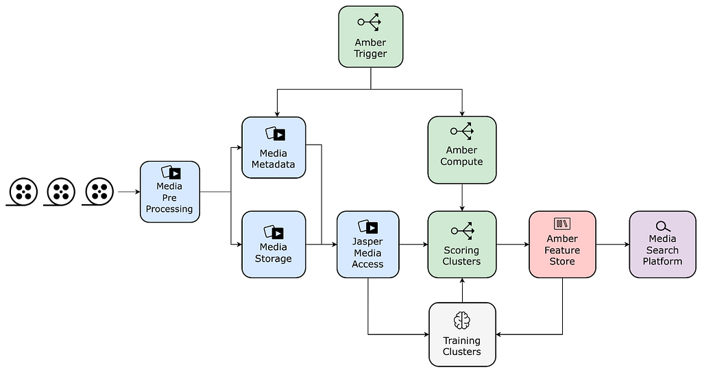
The following figure depicts the new pipeline using the above-mentioned components:
Figure 4 – Match cutting pipeline built using media ML infrastructure components. Interactions between algorithms are expressed as a feature mesh, and each Amber Feature encapsulates triggering and compute.
Conclusion and Future Work
The intersection of media and ML holds numerous prospects for innovation and impact. We examined some of the unique challenges that media ML practitioners face and presented some of our early efforts in building a platform that accommodates the scaling of ML solutions.
In addition to the promotional media use cases we discussed, we are extending the infrastructure to facilitate a growing set of use cases. Here are just a few examples:
ML-based VFX tooling
Improving recommendations using a suite of content understanding models
Enriching content understanding ML and creative tooling by leveraging personalization signals and insights
In future posts, we’ll dive deeper into more details about the solutions built for each of the components we have briefly described in this post.
Today marks an important day for Rapid7, for the state of Florida, and if we may be so bold, for the future of our industry. The announcement of a joint research lab between Rapid7 and the University of South Florida (USF) reaffirms our commitment to driving a deeper understanding of the challenges we face in protecting our shared digital space, while ushering in new talent to ensure that the cyber workforce of tomorrow is as diverse as the individuals who create the shared digital space we set out to protect.
With the Rapid7 Cybersecurity Foundation, we are proud to announce the opening of the Rapid7 Cyber Threat Intelligence Lab in Tampa, at USF. We intend for the lab to be an integral component in real-time threat tracking by leveraging our extensive network of sensors, and incorporating this intelligence not only into our products and customers, but to make actionable indicators available to the wider community. This project also reaffirms our commitment to making cybersecurity more accessible to everyone through our support of research, disclosure, and open source, including projects such as Metasploit, Recog, and Velociraptor to name a few.
We believe that providing USF faculty and students this breadth of intelligence will not only support their journey in learning, but fundamentally provide a clearer path in determining areas to focus in their careers. We are hopeful that working side by side with Rapid7 analysts can help propel this journey, and enhance the meaningful research developed by the university.
As part of the commitment for this investment—and consistent with the guiding principles of the Rapid7 Cybersecurity Foundation—we intend to promote diversity within the cybersecurity workforce. In particular, we plan on opening doors to individuals from historically underrepresented groups within the cybersecurity workforce. With the objective to ensure that research projects are inclusive of those from all backgrounds, we are optimistic that not only will this introduce hands-on technical content to those who may not otherwise have such opportunities, but also, in the longer term, encourage greater diversity within the cybersecurity industry as a whole. We remain steadfast in our commitment to broadening the opportunities within cybersecurity to all those with a passion for creating a more secure and prosperous digital future.
We are deeply thankful to USF for their shared vision, and look forward to a partnership that benefits all students and faculty while producing actionable intelligence that can support the entire internet and the broader industry. Ultimately, the threatscape is such that we recognise no one organization can stop attackers on their own. This partnership remains part of our commitment to establish the relationships between private industry and partners that include academia.
The 6.2 series continues to be fairly calm, and the only real
reason for an rc8 is – as now mentioned several times – just to
make up for some time during the holiday season. Not that we seem
to really have needed it, but there was also no real reason to
deviate from the plan. So here we are.
Ah, football. A beautiful 18 weeks from September to January when we cheer for our favorite teams, eat an uncomfortable amount of dippable appetizers and hand-held foodstuffs, and generally have more exciting Mondays, Thursdays, and Sundays than the rest of the year. And of course, Super Bowl Sunday is the pinnacle of all that joy.
One of the things that we love about football is that it’s given us some incredible moments proving the importance of—you guessed it—backups. Sure, there are only 11 players on the field at any one time, but the team roster has 53 players total, and there’s a reason for that. At any time, the players toward the bottom of the roster could be called up to save the day. And we at Backblaze celebrate times when backups shine.
So, let’s talk about some of our favorite (football) backups of all time and relive those exciting moments.
The Highlight Reel
Brock Purdy, San Francisco 49ers, 2022
We’re based in San Mateo which means we’ve got a lot of Niners fans here at Backblaze. So, you can imagine the joy (and heartbreak) in our office this year. Brock Purdy was the final pick of the 2022 NFL Draft, therefore this season’s Mr. Irrelevant. (We know. It’s kind of mean, but we didn’t make up the name.)
As a third string QB in his rookie season, Purdy likely imagined he’d have little to no play time. Then, first string QB Trey Lance went out with an injury in week two, and Jimmy Garoppolo followed in week 13. Purdy started his first game against the Buccaneers and became the only quarterback in his first career start to beat a team led by Tom Brady.
Backup Steward Yev Pusin rocking his Purdy shirt in the Backblaze offices.
Backblaze’s Ryan Hopkins repping his love for the Chiefs.
After winning the Wild Card game, he suffered an injury to his right elbow, and then his replacement Josh Johnson got a concussion. Sadly, that meant the 49ers were out for the season, but there’s no argument that Purdy outperformed everyone’s expectations. What a backup! (And we hope everyone recovers well.)
We’d like to note here that part of the reason the Niners’ backups got to shine is that the offensive line was so strong this year, so shout out to all the players who put in that work.
The Backup Bottom Line: In our minds, the ability to protect your backups is the hallmark of any good backup strategy.
Max McGee, Green Bay Packers, 1966
This one is truly the stuff of legends, and we need to set the historical stage a bit to truly squeeze the juice, as they say.
The Super Bowl we know and love today pits the two conferences of the NFL against each other. But, back in the day, the Super Bowl was created because oil heir Lamar Hunt created an upstart league called the American Football League (AFL). After a contentious draft, player poaching, and so on, the AFL was looking to prove its legitimacy by challenging the established NFL teams—and so, in 1966, the first Super Bowl was held.
Backblazer Crystal Matina at a game.
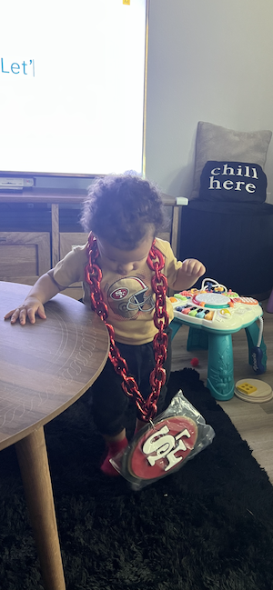
Her daughter Chiara (right) showing Niners love from a young age.
The Green Bay Packers, helmed by the great Vince Lombardi, won the NFL Championship versus the Cowboys and earned the right to face the Kansas City Chiefs in Super Bowl I. Lombardi was reportedly extremely invested in defending the honor of the NFL, and he raised the penalties for breaking curfew to record-high levels. However, that didn’t stop Max McGee.
McGee had gone pro in 1954, and, at that point in 1962, was seemingly close to retirement. That season, he’d only caught four passes total and did not expect to play in the Super Bowl. So, he made plans with two flight attendants and spent the night before the big game drinking, eventually returning to the hotel at 6:30 a.m. game day. (We won’t speculate on what else happened, though Sports Illustrated wrote a fantastic article about McGee.)
In what now only seems fateful, starting receiver Boyd Dowler suffered a shoulder injury in the second drive and was out of the game. A few plays later, hungover and sleep deprived, McGee made a one-handed catch and ran 37 yards to score the first touchdown of the game—the first touchdown in Super Bowl history. By the end of it all, he had 138 receiving yards and two touchdowns, contributing to the Packers’ victory.
McGee went on to retire the following season, but he will never be forgotten.
The Backup Bottom Line: Just like a computer backup, McGee was there when the team most needed him and least suspected it.
Nick Foles, Philadelphia Eagles, 2012–2013
Nick Foles is a great example of someone who found himself bouncing between backup and starter. If you’re not familiar with the Eagles’ 2012 season, their overall record was a dismal four wins, 12 losses. Midseason, starting QB Michael Vick suffered a concussion and Foles got his chance. He started Week 14’s game against the Bucs, and delivered the Eagles’ first win since game four.
When the 2013 season rolled around, the Eagles weren’t quite ready to part ways with Vick. Vick won the starter spot with excellent preseason play, while Foles only gave an average performance. But, when Vick suffered a hamstring injury, Foles again stepped in. By weeks nine and 10, Foles was putting up extremely high passer ratings, and became the first quarterback in NFL history to post passer ratings above 149 in consecutive weeks. He led the team to the NFC East division title and the Wild Card playoffs, and then lost to the Saints who scored a last minute field goal to advance.
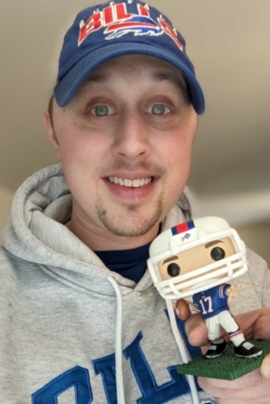
Ryan Ross bringing the Bills pride!
Backblaze Editor Molly Clancy showing up for the Steelers.
Still, the Eagles ended the 2013 season 10–6, a huge improvement from 2012. After an unsuccessful 2014 season, Foles was traded to the Rams. Since then, he’s repeated this same story with the Eagles in 2017 and 2018, but couldn’t seem to make the same magic with the Jaguars (due to injury), the Bears, or the Colts. Ultimately, Foles may be a backup, but he’s responsible for some insane stats—including the best touchdown-interception ratio in the season (2013) and putting up a perfect passer rating in a game (2013, Eagles vs. Raiders).
The Backup Bottom Line: You can never count out your backups. Just when you think they’re an artifact, they bring your best moments back to you.
Darren Sproles, San Diego Chargers, 2005–2011
Speaking of insane stats, let’s talk Darren Sproles. Calling out my bias here, I’m a huge Darren Sproles fan. Also, like Sproles, I spent my youth with the Chargers, then moved onwards and upwards to the Saints. (Yes, San Diego is still salty about the move to L.A. No, I didn’t randomly choose the Saints.)
If you’re unfamiliar with Darren Sproles, he has what is likely the least-probable body type for football, at just 5’6, 190 lbs. I can’t imagine how many times he was likely told to consider football an unrealistic dream by a well-meaning adult in his life. On the other hand, he’s incredibly fast, super powerful in the pocket, and can change directions on a dime. (Plus, it goes without saying he can take a hit.) When Sproles was on the Chargers, word on the street was that he benched more than any player on the O-line.
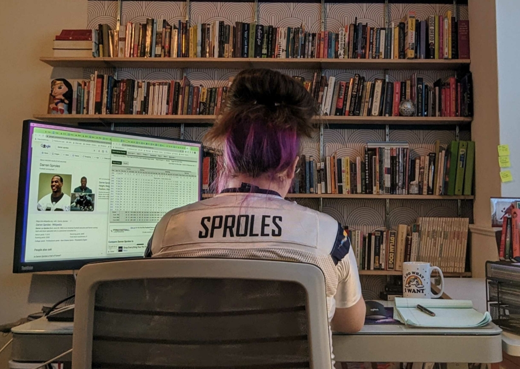
The author in her natural habitat, diligently writing this article for you.
Lily, a very gifted linebacker and roommate of Backblazer Nicole Gale.
At the time, first string running back LaDainian Tomlinson (LT) was—there’s no other word for it—crushing it. Widely regarded as one of the best receivers of all time, he has a career 624 receptions, with 100 of those in the Chargers’ 2001 season. He’s currently 7th place in overall rushing yards, with 13,684 career yards. When Sproles joined the team in 2005, he was third string behind LT and Michael Turner (also an incredible running back, and he almost made our list here).
As Sproles became a big part of the Chargers’ offensive strategy, things became more balanced. That’s not because Darren Sproles was in competition for the top spot; Sproles is a scat back and a specialist in conversions. When it’s third down and you need yards, you want Sproles to have the ball.
Sproles is also an incredible special teams player, so he was often doing double duty in games. When the Chargers played the Colts in 2007, Sproles made history by returning a kickoff and a punt for his first two NFL touchdowns. In 2008, he became the second player in NFL history with 50 rushing yards, 50 receiving yards, and 100 return yards in one game. In 2010, he appeared in all 16 games, with 59 receptions, 50 carries, 51 kick returns, and 24 punt returns.
Sproles went to the Saints in 2011, and in that season, he broke the NFL record for single-season all purpose yardage—2,696 yards. At this point, he’s ranked 6th in career all-purpose yards in NFL history, with 19,696 yards. LaDanian Tomlinson is ranked 10th, with 18,456 yards.
The Backup Bottom Line: Your backups fulfill a totally different purpose than your active data, and often they’re working better (by some measures).
The 49ers fans are back with Backblaze’s Nico Azizian.
Earl Morrall started his career in 1956 as a quarterback and occasional punter. To summarize the first decade or so of his NFL career, he played capably and suffered a few major injuries at key times.
In 1968, he found himself playing for the Baltimore Colts as second string to Hall-of-Famer Johnny Unitas. When Unitas was injured during preseason, Morrall was left to lead the offense, and the team went 13–1 in the regular season. Morrall led the league with 26 touchdowns, and threw for 2,909 yards. After a shutout in the NFL Championship (remember: this is in the days where the American Football League existed), the Colts advanced to Super Bowl III. Widely regarded as one of the greatest upsets in sports history, the Colts lost the Super Bowl after Morrall threw three interceptions, and Unitas came in late in the game and scored the only touchdown of the game. The Colts later won Super Bowl V—which was also the first year after the NFL bought the AFL, and thus the Super Bowl was the ultimate championship in the NFL.
Despite his success, backing up was as far as Morrall would get with the Colts, and in 1972, Morrall went to the Miami Dolphins. Football fans probably already know: In 1972, the Miami Dolphins achieved the first and only perfect season in NFL history. And in game five of that perfect season, starting quarterback Bob Griese broke his ankle—leaving Morrall to start the remaining nine games of the season. In the postseason, he started the Divisional playoff game and the AFC Championship, though Griese came back in the third quarter to finish that one out and then started in the Super Bowl. To make that math simple: That means that in the 1972 Dolphins perfect season, Morrall started 11 of the 17 total games.
Backblaze’s Juan Lopez-Nava shares another perfect thing in football: his pup and dedicated 49ers fan, Mila.
Morrall went on to retire from the Dolphins in 1977 with only sporadic playtime marking the time in between.
The Backup Bottom Line: It just goes to show: having a great backup means that you can rely on the system to work, even if key parts of your initial strategy go down.
Even Our Backup Stories Had Backups
When we first started talking about this article, we were sure there’d be great backup stories, but it’s incredible how many we found. We have a whole list of players whose moments didn’t get highlighted in this piece simply because we ran out of space, and, frankly, some of them are just as impressive (maybe even more so?) when compared to those above. If you want to do some further investigation, check out Geno Smith, Teddy Bridgewater, Michael Turner, Kurt Warner, Jeff Hofstetler, Trey McBride, Cordarrelle Patterson, Devin Hester—and then let us know who else you turn up in the comments section, because we’re sure we missed some good stories.
Pwnagotchi is an A2C-based “AI” leveraging bettercap that learns from its surrounding WiFi environment to maximize crackable WPA key material it captures
Тази седмица спокойно можеше и да не се състои. Започна с опустошителното земетресение в Турция и Сирия, отнело живота на хиляди хора, и завърши с новината, че още един българин е бил убит от съседа си, защото мига шумно. Предишният случай беше от ноември миналата година, когато Константин Дамов (62 г.) след многобройни междусъседски разпри застреля 41-годишния баща на три деца Иво Андреев. Поводът, твърди се, е някаква врата. Може и да е онази същата, зад която упорито крием обществените си угризения, че допускаме да се случва всичко това.
Паралелно с трагедията на местно ниво, където, изглежда, всички сме съучастници, вървят и световните процеси, в които също се включваме посвоему. Тази седмица Александър Нуцов се опитва да опише как би изглеждал мирът след края на войната в Украйна и какво ще е състоянието на международната система. В текста „Устойчив мир или нова желязна завеса“ той обръща внимание и на реалните отношения между ЕС, НАТО и Русия. Древните са казали: „Ако искаш мир, готви се за война“, но не е лошо да се има предвид и обратният вариант: „Ако искаш война, готви се за мир.“ Александър обяснява защо.
Оставяме международното положение леко встрани, правим един пирует и се приземяваме не чак толкова елегантно в блатото на българския политически живот, където редиците се стягат за нови избори. Емилия Милчева повдига въпроса как се избират от партиите онези, които ще избираме после ние – с други думи, каква е механиката, с която ще се запълват новите партийни листи. Във „Вот 2023. „Мат’рял“ за листи или хора за избиране“ отново можем да си припомним къде живеем (в случай че ни се е удала възможност да забравим), като обърнем внимание на следното: няма демократични регламенти и добри практики за номинации на кандидати и всичко изглежда като кастинг, а не като реален политически процес.
Като казах „политически процес“, ми се прииска да направя очевидната констатация, че политиката в България е населявана от всякакви „политически животни“ (да ме прощава Аристотел) и това може би има известна очарователност, особено когато ги „изследваме“ през балоните в социалните си мрежи. Но когато политиците нападат с безпочвени обвинения журналисти, защото журналистите се осмеляват да си вършат работата, изглежда, че нещата леко излизат от коловозите на основополагащите принципи на демократичните общества, сред които са свободата на словото и независимостта на медиите.
Буквално преди дни Емилия Милчева беше атакувана от политическа партия „Възраждане“ за свой репортаж в „Дойче Веле“, който разглежда какви са хората, подписващи се против еврото, и какви са техните съображения. Емилия пита, записва отговорите и без да знае, се оказва нарушител на обществения ред. После, разбира се, има пресконференция на „Възраждане“, на която представители на партията „разобличават“ Емилия Милчева като лице, минало през много „българоезични американски медии в България“, пратено да провокира. Истината е, че тук вече всяко по-настоятелно задаване на въпроси се смята за лошо възпитание, както казва журналистката Миролюба Бенатова в едно свое интервю. Така че каквото и да се каже по този въпрос, все ще е провокация. Затова спирам, понеже основната цел на „Тоест“ е да ни провокира да мислим, а не да правим пресконференции.
Българското участие във Венецианското архитектурно биенале е тема, по която със сигурност тепърва ще се мисли и говори. България не се е представяла на този форум от 15 години. Повечето кандидати, явили се на конкурса за избор на наш участник, са показали съвсем адекватни предложения, както пише в текста си „Венеция, България и изоставените сгради“ арх. Анета Василева. Този избор не минава и без скандал или поне без опит за такъв. В крайна сметка е излъчен проектът на POV Architects „Образованието е придвижването от тъмнина към светлина“, поставящ фокус върху изоставените сгради на стари училища в България. Какъв е контекстът, в който ще се представи нашето предложение, какво представлява то и какви са възможностите за неговото по-добро реализиране, разказва арх. Василева.
От тъмнината към светлината със сигурност ни придвижват и книгите. Особено когато осветляват истории „от архивите“. Тази седмица тръгваме по буквите със Зорница Христова, която ни представя „Кой е Сава Попов? Отключването на един архив“ от Антон Стайков и Свобода Цекова, „Оловна тишина. Историята на един разстрел“ от Ивайла Александрова и „Световна литература. Космополитизъм. Изгнание“ от Галин Тиханов.
Първата книга разказва за писателя и журналист Сава Попов. Неговата история остава някак неглижирана, но сега се появява като резултат от изключително задълбочено изследване на архивите на писателя „с обаянието на автентичния материал, но и с осезаемо разказваческо умение“, както пише Зорница.
„Оловна тишина“ е още един изследователски труд, целящ да разкаже истинската история, а не кратката ѝ версия за пред знамето. Ивайла Александрова се заема да разгледа документите по делото на Никола Вапцаров и да ги предостави като контрааргумент срещу всички клишета за него. Добре е да се отбележи, че „Оловна тишина“ не е съд над Вапцаров. Особено пък като поет“, както казва Зорница Христова.
Тази седмица „По буквите“ завършва с представяне на „Световната литература. Космополитизъм. Изгнание“ на Галин Тиханов, в която участва и Марин Бодаков. Историята на идеите е сърцевината на книгата на проф. Тиханов, литературовед, член на Британската академия. Какво всъщност е космополитизмът, ако си представим понятието като персонаж, и къде се крие политическият потенциал на тази книга – прочетете в текста на Зорница Христова.
To provide the best experiences, we use technologies like cookies to store and/or access device information. Consenting to these technologies will allow us to process data such as browsing behavior or unique IDs on this site. Not consenting or withdrawing consent, may adversely affect certain features and functions.
Functional
Always active
The technical storage or access is strictly necessary for the legitimate purpose of enabling the use of a specific service explicitly requested by the subscriber or user, or for the sole purpose of carrying out the transmission of a communication over an electronic communications network.
Preferences
The technical storage or access is necessary for the legitimate purpose of storing preferences that are not requested by the subscriber or user.
Statistics
The technical storage or access that is used exclusively for statistical purposes.The technical storage or access that is used exclusively for anonymous statistical purposes. Without a subpoena, voluntary compliance on the part of your Internet Service Provider, or additional records from a third party, information stored or retrieved for this purpose alone cannot usually be used to identify you.
Marketing
The technical storage or access is required to create user profiles to send advertising, or to track the user on a website or across several websites for similar marketing purposes.