Tag Archives: Amazon Redshift

Dream11’s journey to building their Data Highway on AWS

Post Syndicated from Pradip Thoke original https://aws.amazon.com/blogs/big-data/dream11s-journey-to-building-their-data-highway-on-aws/

This is a guest post co-authored by Pradip Thoke of Dream11. In their own words, “Dream11, the flagship brand of Dream Sports, is India’s biggest fantasy sports platform, with more than 100 million users. We have infused the latest technologies of analytics, machine learning, social networks, and media technologies to enhance our users’ experience. Dream11 is the epitome of the Indian sports technology revolution.”

Since inception, Dream11 has been a data-driven sports technology brand. 

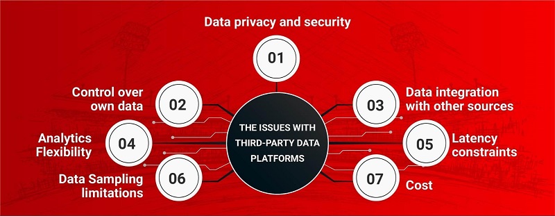
Since inception, Dream11 has been a data-driven sports technology brand. The systems that power Dream11, including their transactional data warehouse, run on AWS. As Dream11 hosts fantasy sports contests that are joined by millions of Indian sports fans, they have large volumes of transactional data that is organized in a well-defined Amazon Redshift data warehouse. Previously they were using 3rd party services to collect, analyze and build models over user interaction data combined with transactional data. Although this approach was convenient, it presented certain critical issues:

  • The approach wasn’t conducive to 360-degree user analytics. Dream11’s user interactions data wasn’t present on the cloud, where the rest of Dream11’s infrastructure and data were present (AWS, in this case). To get a complete picture of a user’s experience and journey, the user’s interaction data (client events) needs to be analyzed alongside their transactional data (server events). This is known as 360-degree user analytics.
  • It wasn’t possible to get accurate user journey funnel reports. Currently, there are limitations with every tool available on the market with respect to identifying and mapping a given user’s actions across multiple platforms (on the web, iOS, or Android), as well as multiple related apps. This use case is specifically important if your company is a parent to other companies.
  • The statistics on user behavior that Dream11 was getting weren’t as accurate as they wanted. Some of the popular services they were using for web & mobile analytics use the technique of sampling to be able to deal with high volumes of data. Although this is a well-regarded technique to deal with high volumes of data and provides reasonable accuracy in multiple cases, Dream11 wanted statistics to be as accurate as possible.
  • The analytics wasn’t real-time. Dream11 experiences intense use by their users just before and during the real-life sports matches, so real-time and near-real-time analytics is very critical for them. This need wasn’t sufficiently met by the plethora of services they were using.
  • Their approach was leading to high cost for custom analytics for Dream11’s user interactions data, consisting of hundreds of event types. Serverless query engines typically charge by the amount of data scanned and so it can get very expensive if events data isn’t organized properly in separate tables in a data lake to enable selective access.

All these concerns and needs, led Dream11 to conclude that they needed their own centralized 360-degree analytics platform.

All these concerns and needs, led Dream11 to conclude that they needed their own centralized 360-degree analytics platform. Therefore, they embarked on the Data Highway project on AWS.

This project has additional advantages. It is increasingly becoming important to store and process data securely. Having everything in-house can help Dream11 with data security and data privacy objectives. The platform enables 360-degree customer analytics, which further allows Dream11 to do intelligent user segmentation in-house and share only those segments (without exposing underlying transactional or interactions data) with third-party messaging service providers. 

Design goals

Dream11 had the following design goals for the project:

  • The system should be easy to maintain and should be able to handle a very high volume of data, consisting of billions of events and terabytes of data daily.
  • The cost should be low and should be pay-as-you-go.
  • Dream11’s web and mobile developers regularly create new types of events to capture new types of interactions. Whenever they add new types of events, they should be immediately available in the system for analytics, and their statistics should immediately reflect in relevant dashboards and reports without any human intervention.
  • Certain types of statistics (such as concurrency) should be available in real-time and near-real time—within 5 minutes or less.
  • Dream11 should be able to use custom logic to calculate key statistics. The analytics should be accurate—no more sampling.
  • The data for various events should be neatly organized in separate tables and analytics-friendly file formats.
  • Although Dream11 will have a common data lake, they shouldn’t be constrained to use a single analytics engine for all types of analytics. Different types of analytics engines excel for different types of queries.
  • The Product Management team should have access to views they commonly use in their decision-making process, such as funnels and user flow diagrams.
  • The system should be extensible by adding lanes in the system. Lanes allow you to reuse your basic setup without mixing events data for different business units. It also potentially allows you to study user behavior across different apps.
  • The system should be able to build 360-degree user profiles
  • The system should provide alerting on important changes to key business metrics.
  • Last but not the least, the system should be secure and reliable with 6 nines of availability guarantee.

Data Highway architecture

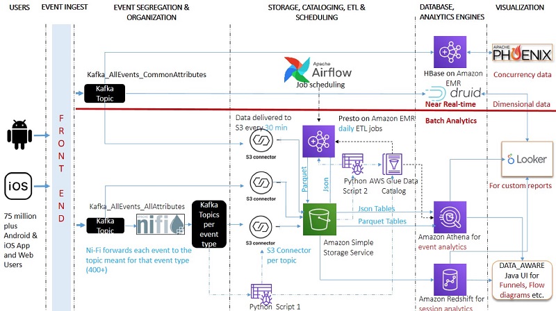
In less than 3 months, Dream11’s data team built a system that met all the aforementioned goals. The following diagram shows the high-level architecture.

The following diagram shows the high-level architecture.

For this project, they used the following components:

The rest of this post explains the various design choices and trade-offs made by the Dream11’s data engineers. 

Event ingestion, segregation, and organization

Dream11 has several hundred event types. These events have common attributes and specific attributes. The following diagram shows the logical structure of these events.

The following diagram shows the logical structure of these events.

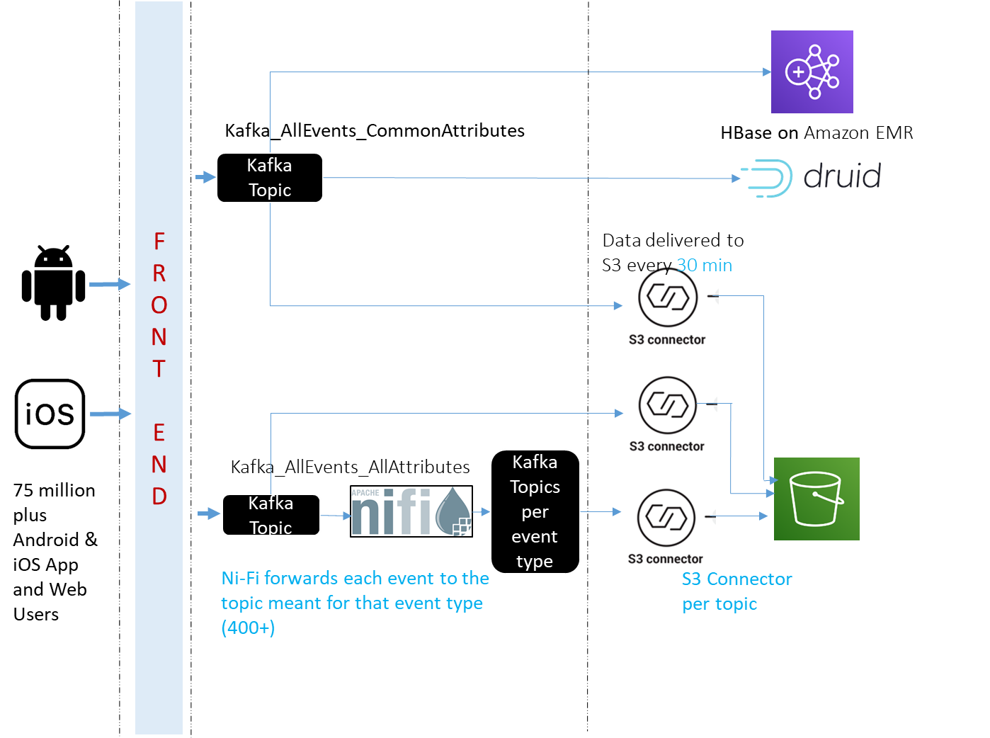
When the front end receives an event, it saves fields up to common attributes into a message and posts it to Kafka_AllEvents_CommonAttributes. This Kafka topic is the source for the following systems:

  • Apache HBase on Amazon EMR – Provides real-time concurrency analytics
  • Apache Druid – Provides near real-time dimensional analytics
  • Amazon Redshift – Provides session analytics

The front end also saves events, as they are, into Kafka_AllEvents_AllAttributes. These events are further picked by Apache Ni-Fi, which forwards them to their respective topics. Apache Ni-Fi supports data routing, transformation, and system mediation logic using powerful and scalable directed graphs. Data is transformed and published to Kafka by using a combination of RouteOnAttribute and JoltTransformJSON processors (to parse JSON). Apache Ni-Fi basically reads event names and posts to the Kafka topic with matching names. If Kafka doesn’t have a topic with that name, it creates a new topic with that name. You can configure your Kafka brokers to auto-create a topic when a message is received for a non-existent topic.

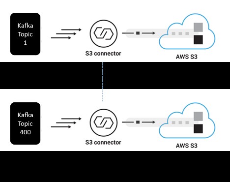
The following diagram illustrates the Amazon S3 sink connector per Kafka topic.

  The following diagram illustrates the Amazon S3 sink connector per Kafka topic.

The following diagram summarizes the overall design of the system for event ingestion, segregation, and organization.


The following diagram summarizes the overall design of the system for event ingestion, segregation, and organization.

Storage, cataloging, ETL, and scheduling

In this section, we discuss how Dream11 updates their AWS Glue Data Catalog, performs extract, transform, and load (ETL) jobs with Amazon EMR Presto, and uses Apache Airflow for schedule management.

Updating the AWS Glue Data Catalog with metadata for the target table

The AWS Glue Data Catalog provides a unified metadata repository across a variety of data sources and data formats. It provides out-of-the-box integration with Amazon S3, Amazon Relational Database Service (Amazon RDS), Amazon Redshift, Amazon Redshift Spectrum, Athena, Amazon EMR, and any application compatible with the Apache Hive metastore. You can create your table definitions one time and query across engines. For more information, see FAQ: Upgrading to the AWS Glue Data Catalog.

Because this Data Catalog is accessible from multiple services that were going to be used for the Data Highway project, Dream11 decided to use it to register all the table definitions.

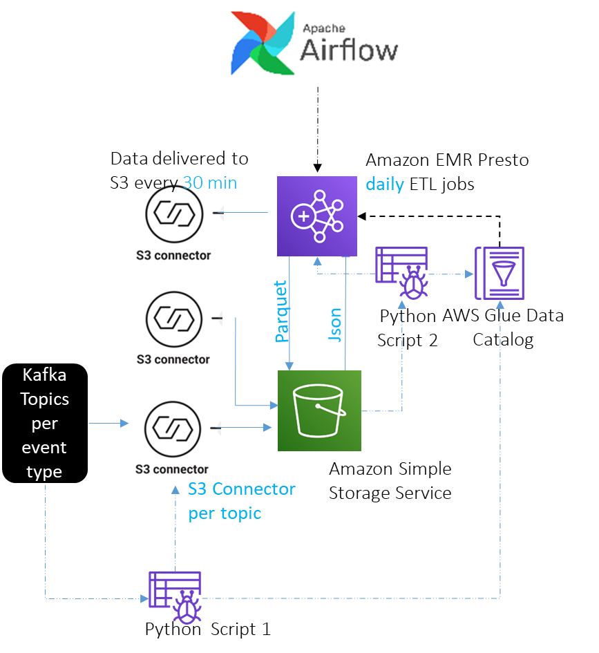
Registering tables with AWS Glue Data Catalog is easy. You can use an AWS Glue crawler. It can infer schema from files in Amazon S3 and register a table in the Data Catalog. It works quite well, but Dream11 needed additional actions, such as automatically configuring Kafka Amazon S3 sink connectors etc. Therefore, they developed two Python based crawlers.

The first Python based crawler runs every 2 hours and looks up Kafka topics. If it finds a new topic, it configures a Kafka Amazon S3 connector sink to dump its data to Amazon S3 every 30 minutes in JSON Gzip format. It also registers a table with Glue Data Catalog so that users can query the JSON data directly, if needed. 

The second Python based crawler runs once a day and registers a corresponding table for each new table created that day to hold flattened data (Parquet, Snappy). It infers schemas and registers tables with the Data Catalog using its Table API. It adds customization needed by the Dream11 team to the metadata. It then creates Amazon EMR Presto ETL jobs to convert JSON, Gzip data to Parquet, Snappy, and registers them with Apache Airflow to run every 24 hours.

ETL with Amazon EMR Presto

Dream11 has a multi node, long-running, multi-purpose EMR cluster. They decided to run scheduled ETL jobs on it for the Data Highway project.

ETL for an event table involves a simple SELECT FROM -> INSERT INTO command to convert JSON (Gzip) to Parquet (Snappy). Converted data takes up to 70% less space, results in 10 times improvement in Athena query performance. ETL happens once a day. Tables are partitioned by day.

Data received on Kafka_AllEvents_CommonAttributes topic is loaded to Redshift. ETL involves SELECT FROM -> INSERT INTO to convert JSON (Gzip) to CSV, followed by Amazon Redshift COPY.

Apache Airflow for schedule management

Apache Airflow is an open-source tool for authoring and orchestrating big data workflows. With Apache Airflow, data engineers define direct acyclic graphs (DAGs). DAGs describe how to run a workflow and are written in Python. Workflows are designed as a DAG that groups tasks that run independently. The DAG keeps track of the relationships and dependencies between tasks.

Dream11 uses Apache Airflow to schedule Python scripts and over few hundred ETL jobs on Amazon EMR Presto to convert JSON (Gzip) data for over few hundred events to Parquet (Snappy) format, and converts JSON data containing common attributes for all events to CSV before loading to Amazon Redshift. For more information, see Orchestrate big data workflows with Apache Airflow, Genie, and Amazon EMR: Part 1.

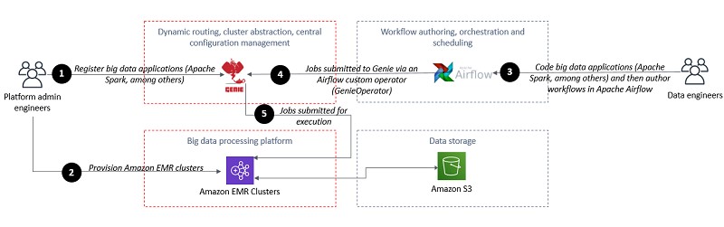
The following diagram shows the workflow to connect Apache Airflow to Amazon EMR.

The following diagram shows the workflow to connect Apache Airflow to Amazon EMR.

The following diagram summarizes the overall design of the system for storage, cataloging, ETL, and scheduling.

The following diagram summarizes the overall design of the system for storage, cataloging, ETL, and scheduling. 

Real-time and near-real-time analytics

In this section, we discuss the real-time and near-real-time analytics performed on Dream11’s data.

Concurrency analytics with Apache Druid

Apache Druid is an OLAP-style data store. It computes facts and metrics against various dimensions while data is being loaded. This avoids the need to compute results when a query is run.

Dream11’s web and mobile events are loaded from the Kafka_AllEvents_CommonAttributes topic to Apache Druid with the help of the Apache Druid Kafka indexing service. Dream11 has a dashboard with different granularity levels and dimensions such as app version, org, and other dimensions present in the common event attributes list.

Finding active users with Amazon EMR HBase

Dream11 also needs to identify individual active users at any given time or during a given window. This is required by other downstream teams such as the Data Science team and Digital User Engagement team.

With the help of a Java consumer, they push all events from the Kafka_AllEvents_ CommonAttributes topic to HBase on an EMR cluster with just required user dimensions. They can query the data in HBase with SQL syntax supported by the Apache Phoenix interface. 

Session analytics with Amazon Redshift

Dream11 maintains their transactional data warehouse on Amazon Redshift multi node cluster. Amazon Redshift allows them to run complex SQL queries efficiently. Amazon Redshift would have been a natural choice for event analytics for hundreds of event types. However, in Dream11’s case, events data grows very rapidly and this would be a lot of data in Amazon Redshift. Also, this data loses its value rapidly as time passes (relatively speaking) compared with transactional data. Therefore, they decided to do only session analytics in Amazon Redshift to benefit from its complex SQL query capabilities and to do analytics for individual events with the help of Athena (which we discuss in the next section).

Data received on Kafka_AllEvents_CommonAttributes is loaded into Amazon S3 every 30 minutes by the associated kafka connector sink. This data is in JSON format with Gzip compression. Every 24 hours, a job runs on Amazon EMR Presto that flattens this data into CSV format. The data is loaded into Amazon Redshift with the COPY command. The data gets loaded first into a staging table. Data in the staging table is aggregated to get sessions data. Amazon Redshift already has transactional data from other tables that, combined now with the session data, allows Dream11 to perform 360-degree user analytics. They can now easily segment users based on their interactions data and transactions data. They can then run campaigns for those users with the help of messaging platforms. 

Event analytics with Athena

Dream11 uses Athena to analyze the data in Amazon S3. Athena is an interactive query service that makes it easy to analyze data in Amazon S3 using standard SQL. Athena is serverless, so there is no infrastructure to manage, and you pay only for the queries that you run. It made perfect sense to organize data for over hundreds of event tables in Amazon S3 and analyze them with Athena on demand.

With Athena, you’re charged based on the amount of data scanned by each query. You can get significant cost savings and performance gains by compressing, partitioning, or converting your data to a columnar format, because each of those operations reduces the amount of data that Athena needs to scan to run a query. For more information, see Top 10 Performance Tuning Tips for Amazon Athena.

As discussed before, Dream11 has registered over hundreds of tables for events data in JSON format, and similar number of tables for events data in Parquet format with the AWS Glue Data Catalog. They observed a performance gain of 10 times on conversion of data format to Parquet, and an 80% savings in space. Data in Amazon S3 can be queried directly through the Athena UI with SQL queries. The other option they use is connecting to Athena using a JDBC driver from Looker and their custom Java UI for the Data Aware project.

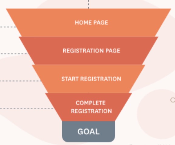
Athena helps Dream11 produce funnel analytics and user path analytics reports and visualizations.

  Athena helps Dream11 produce funnel analytics and user path analytics reports and visualizations.

 The following diagram summarizes the overall design of the system for real-time and near-real-time analytics and visualization.

 The following diagram summarizes the overall design of the system for real-time and near-real-time analytics and visualization.


Conclusion

This architecture has enabled Dream11 to achieve all the design goals they set out with. Results of analytics for real-time requirements are available under millisecond latency, and the system costs 40% less than the previous system. Analytics is performed with all the data without sampling, so results are accurate and reliable. All the data and analytics engines are within Dream11’s AWS account, improving data security and privacy.

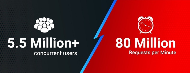
As of this writing, the system handles 14 TB of data per day and it has served 80 million requests per minute at peak during Dream11 IPL 2020.

Doing all their analytics in-house on AWS has not just improved speed, accuracy, and data security, it has also enabled newer possibilities. Now Dream11 has a 360-degree view of their users. They can study their users’ progress across multiple platforms – web, Android, and IOS. This new system is enabling novel applications of machine learning, digital user engagement, and social media technologies at Dream11.


About the Authors

Pradip Thoke is a AVP Data Engineering at Dream11 and leads their Data Engineering team. The team involved in this implementation includes Vikas Gite, Salman Dhariwala, Naincy Suman, Lavanya Pulijala, Ruturaj Bhokre, Dhanraj Gaikwad, Vishal Verma, Hitesh Bansal, Sandesh Shingare, Renu Yadav, Yash Anand, Akshay Rochwani, Alokh P, Sunaim and Nandeesh Bijoor.


Girish Patil is a Principal Architect AI, Big Data, India Scale Apps for Amazon.

Building high-quality benchmark tests for Amazon Redshift using Apache JMeter

Post Syndicated from Asser Moustafa original https://aws.amazon.com/blogs/big-data/building-high-quality-benchmark-tests-for-amazon-redshift-using-apache-jmeter/

In the introductory post of this series, we discussed benchmarking benefits and best practices common across different open-source benchmarking tools. As a reminder of why benchmarking is important, Amazon Redshift allows you to scale storage and compute independently, and for you to choose an appropriately balanced compute layer, you need to profile the compute requirements of various production workloads. Existing Amazon Redshift customers also desire an approach to scale up with eyes wide open, and benchmarking different Amazon Redshift cluster configurations against various production workloads can help you appropriately accommodate workload expansion. In addition, you may also use benchmark tests to proactively monitor a production cluster’s performance in real time.

For prospective Amazon Redshift customers, benchmarking Amazon Redshift is often one of the main components of evaluation and a key source of insight into the price-to-performance ratio of different Amazon Redshift configurations.

Open-source tools, with their cost-efficiency and vendor neutrality, are often the preferred choice for profiling your production workloads and benchmark tests. However, best practices for using these tools are scarce, possibly resulting in flawed compute profiles, flawed benchmark results, customer frustration, or bloated timelines.

As mentioned, this series is divided into multiple installments, with the first installment discussing general best practices for benchmarking, and the subsequent installments discussing the strengths and challenges with different open-source tools such as SQLWorkbench, psql, and Apache JMeter. In this post, we discuss benchmarking Amazon Redshift with the Apache JMeter open-source tool.

One final point before we get started: there is a lot that could be said about benchmarking—more than can be accommodated in a single post. Analytics Specialists Solutions Architects such as myself frequently and happily engage with current and prospective customers to help you evaluate your benchmarking strategy and approach at no charge. I highly recommend you take advantage of that benefit by reaching out to your AWS account SA.

Apache JMeter

Apache JMeter is an open-source load testing application written in Java that you can use to load test web applications, backend server applications, databases, and more. You can run it on Windows and a number of different Linux/UNIX systems; for this post we run it in a Windows environment. To install Apache JMeter on a Windows EC2 machine, complete the following steps:

  1. Launch a Windows EC2 instance using a Windows Server AMI (such as Microsoft Windows Server 2019 Base).
  2. Connect via RDP to the Windows EC2 Instance (RDP for macOS can be downloaded from Apple’s App Store).
  3. Download and unzip the Apache JMeter .zip file from the Apache JMeter download page.
  4. Download the Redshift JDBC driver and add the driver .jar file to JMeter’s /lib When setting up the JDBC connection in the JMeter GUI, use com.amazon.redshift.jdbc.Driver as the driver class name).
  5. Download the Apache Plugins Manager .jar file to JMeter’s /lib/ext The Apache Plugins Manager enables additional crucial functionality in Apache JMeter for benchmark testing (such as Ultimate Thread Group).
  6. Increase the JVM heap size for Apache JMeter by changing the corresponding JVM parameters in the jmeter.bat file located in the Apache JMeter /bin folder. For example, see the following code:
    edit C:\Dev\apache-jmeter-5.1.1\bin\jmeter.bat rem set HEAP=-Xms1g -Xmx1g -XX:MaxMetaspaceSize=256m set HEAP=-Xms5g -Xmx5g -XX:MaxMetaspaceSize=1g

  1. Choose the jmeter.bat file (double-click) to start Apache JMeter.

Apache JMeter supports both GUI and CLI modes, and although you may find the Apache JMeter GUI straightforward with a relatively small learning curve, it’s highly recommended that you use the Apache JMeter GUI primarily for defining benchmark tests, and perhaps running small-to-medium-sized benchmark tests. For large load tests, it’s highly recommended that you use the Apache JMeter CLI to minimize the risk of the Apache JMeter GUI exhausting its host’s compute resources, causing it to enter a non-responsive state or fail with an out-of-memory error. Using the CLI for large load tests also helps minimize any impact on the benchmark results.

In the following example, I demonstrate creating a straightforward load test using both the Apache JMeter GUI and CLI. The load test aims to measure query throughput while simulating 50 concurrent users with the following personas:

  • 20 users submit only small queries, which are of low complexity and typically have a runtime of 0–30 seconds in the current system, such as business intelligence analyst queries
  • 20 users submit only medium queries, which are of moderate complexity and typically have a runtime of 31–300 seconds in the current system, such as data engineer queries
  • 10 users submit only large queries, which are very complex and typically have a runtime over 5 minutes in the current system, such as data scientist queries

The load test is configured to run for 15 minutes, which is a pretty short test duration, so you can increase that setting to 30 minutes or more. We rely on JMeter’s query throughput calculation, but we can also manually compute query throughput from the runtime metadata that is gathered if we so desire.

For this post, I skip over discussing the possible Amazon Redshift cluster tweaks that you could use to squeeze every drop of performance out of Amazon Redshift, and instead rely on the strength of its default state to be optimized to achieve excellent query throughput on diverse workloads.

Apache JMeter has a number of building blocks, such as thread groups, that can be used to define a wide variety of benchmark tests, and each building block can have a number of community implementations (for example, Arrivals Thread Group or Ultimate Thread Group).

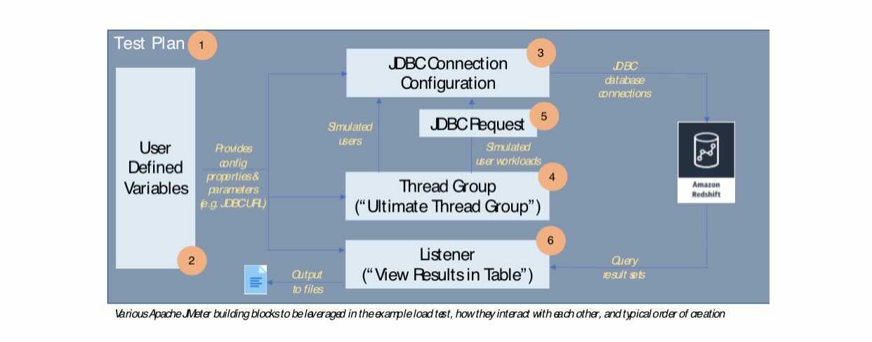
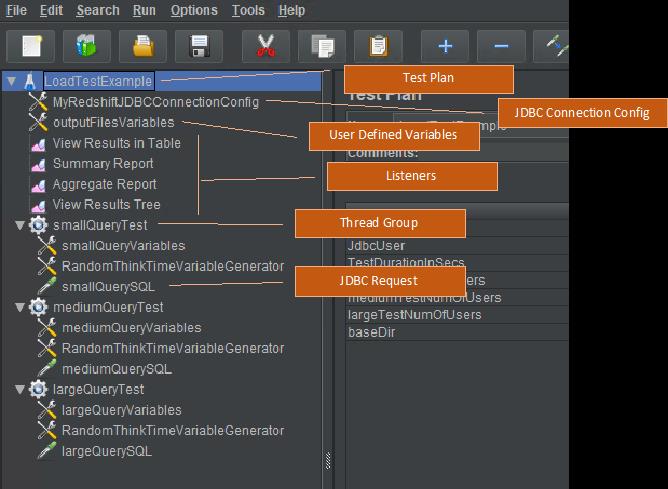
The following diagram provides a basic illustration of the various Apache JMeter building blocks to be leveraged in this load test, how they interact with each other, and the typical order in which are they created; in some cases, I mention the specific implementation of the building block to be used in parenthesis (such as Ultimate Thread Group).

The following table delves deeper into the purpose that each building block serves in our load test.

Apache JMeter Component Purpose
Test Plan Represents an atomic test case (simulate 50 users concurrently querying a Redshift cluster with twice the baseline node count)
JDBC Connection Configuration Represents all the JDBC information needed to connect to the Amazon Redshift cluster (such as JDBC URL, username, and password)
User Defined Variables A collection of key-value pairs that can be used as parameters throughout the test plan and make it easier to maintain or change the test behavior
Listener Captures and displays or writes test output such as SQL result sets
Thread Group A simulated group of users that perform the test function (submit a SQL query)
JDBC Request The action to be taken by the simulated users (SQL query text)

Apache JMeter (GUI)

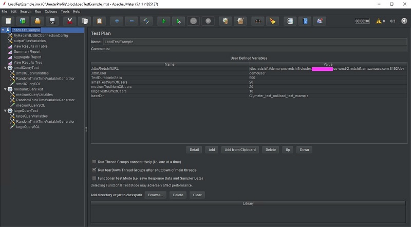
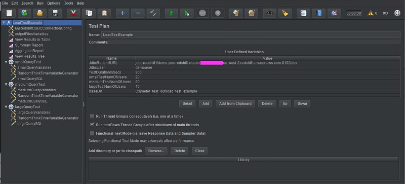
The following screenshot is the resulting load test.

The following screenshot is the resulting load test.

The following screenshot provides a close up of the building block tree.

The following screenshot provides a close up of the building block tree.

In the following sections, we examine each building block in greater detail.

Test Plan

The test plan serves as the parent container for our entire benchmark test, and we can change its name in the visual tree that appears in the Apache JMeter GUI by editing the Name field.

I take advantage of the User Defined Variables section to set my own custom variables that hold values needed by all components in the test case, such as the JDBC URL, test duration, and number of users submitting small, medium, and large queries. The baseDir variable is actually a variable that is intended to be embedded in other variables, rather than directly referenced by other test components. I left all other settings at their default on this page.

The baseDir variable is actually a variable that is intended to be embedded in other variables, rather than directly referenced by other test components.

JDBC Connection Configuration

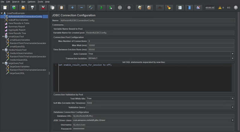
We use the JDBC Connection Configuration building block to create a database connection pool that is used by the simulated users to submit queries to Amazon Redshift. The value specified in Variable Name for created pool is the identifier that is used to reference this connection pool in other JMeter building blocks. In this example, I named it RedshiftJDBCConfig.

By setting the Max Number of Connections to 0, the connection pool can grow as large as it needs to. That may not be the desired behavior for all test scenarios, so be sure to set it as you see fit.

In the Init SQL statements section, I provide an example of how to use SQL to disable the result set cache in Amazon Redshift for every connection created, or perform other similar initialization code.

Towards the end, I input the database JDBC URL (which is actually a variable reference to a variable defined in the test plan), JDBC driver class name, and database username and password. I left all other fields at their default on this page.

I left all other fields at their default on this page.

User Defined Variables

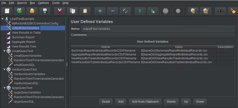
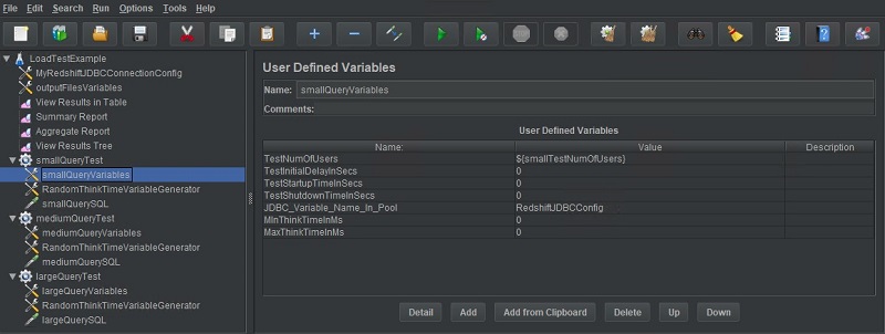
You can add a User Defined Variables building block in several places, and it’s best to use this capability to limit the scope of each variable. For this post, we use an instance of the User Defined Variables building block to hold the output file names of each listener in this test plan (if you look closely, you can see the values of these variables reference the baseDir variable, which was defined in our test plan). You can also notice three other instances of the User Defined Variables building block for the small, medium, and large thread groups—again so that the scope of variables is kept appropriately narrow.

You can add a User Defined Variables building block in several places, and it’s best to use this capability to limit the scope of each variable.

Listeners

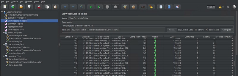
Listeners control where test output is written and how it’s processed. There are many different kinds of listeners that, for example, allow you to capture your test output as a tree, table, or graph. Other listeners can summarize and aggregate test metadata (such as the number of test samples submitted during the test). I choose to add several listeners in this test plan just for demonstration, but I have found the listeners Aggregate Report and View Results in Table to be most helpful to me. The following screenshot shows the View Results in Table output.

The following screenshot shows the View Results in Table output.

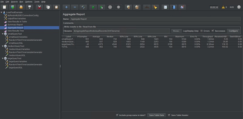
The following screenshot shows the Aggregate Report output.

The following screenshot shows the Aggregate Report output.

You can also save output from listeners after a test run to a different file through the JMeter menu.

Thread group: Ultimate Thread Group

A thread group can be thought of as a group of simulated users, which is why for this post, I create three separate thread groups: one to represent each of three previously mentioned user personas being simulated (small, medium, and large). Each thread group is named accordingly.

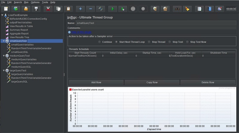
We use the Thread Schedule section to control how many users should be created and at what time interval. In this test, I chose to have all 20 small users created at start time without any delays. This is achieved by a one-row entry in the Thread Schedule and setting the Start Threads Count thread group property to 20 users (or the matching variable, as we do in the following screenshot).

We use the Thread Schedule section to control how many users should be created and at what time interval.

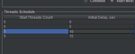
Alternatively, I could stagger user creation by creating multiple rows and setting the Initial Delay sec field to control each row’s startup delay. With the row entries in the following screenshot, an additional five users are created every 5 seconds.

With the row entries in the following screenshot, an additional five users are created every 5 seconds.

Thread group: User Defined Variables

An additional User Defined Variables instance is added to each of the three thread groups to hold the variables in their individual scope, or that would preferably be configurable at an individual thread group level. For this post, I make the JDBC Connection Configuration a variable so that it’s customizable for each individual thread group (JDBC_Variable_Name_In_Pool). This allows me to, for example, rapidly switch two different test clusters.

An additional User Defined Variables instance is added to each of the three thread groups to hold the variables in their individual scope.

JDBC Request

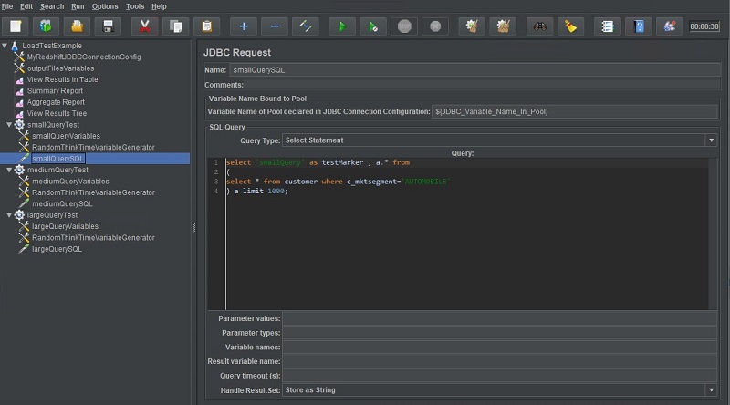
The JDBC Request can be thought of as the benchmark query or SQL test query to be submitted non-stop by each simulated user in this thread group. To configure this JDBC Request, I specified the appropriate JDBC Connection Configuration and some very simple test SQL. I could have also used Apache JMeter’s ability to parameterize queries so that they vary from one iteration to another using a predetermined set of parameter values. For example, for the SQL statement select * from customer where cust_id=<some value>, Apache JMeter could be configured to set the value in the filter clause to a randomly chosen value from a pre-compiled list of filter values for each sample submission. I left all other settings at their default.

The JDBC Request can be thought of as the benchmark query or SQL test query to be submitted non-stop by each simulated user in this thread group.

Apache JMeter (CLI)

The Apache JMeter GUI saves test plans in .jmx files that can be used to run the same test plan in Apache JMeter’s console mode. The following CLI command demonstrates how you can use the LoadTestExample.jmx file that was created in the previous steps using the GUI to run the same load test:

> <jmeter_install_dir>\bin\jmeter -n -t LoadTestExample.jmx -e -l test.out

The sample output is from a 30-second run of LoadTestExample.jmx.

The sample output is from a 30-second run of LoadTestExample.jmx.

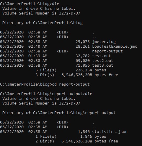
After the test has completed, several output files are created, such as a JMeter application log, query output files from the listeners (if any), and test statistics from listeners (if any). For this post, the statistical metrics captured for the test run are located in a JSON file inside the report-output directory. See the following screenshot.

For this post, the statistical metrics captured for the test run are located in a JSON file inside the report-output directory.

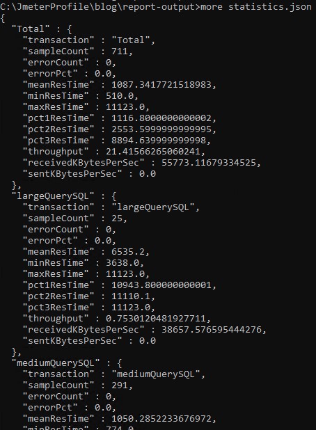
The \report-output\statistics.json file captures a lot of useful metrics, such as the total samples (like SQL queries) submitted during the test duration, achieved query throughput, and number of small, medium, and large queries and their individual throughput. The following screenshot shows a sampling of the data from statistics.json.

The following screenshot shows a sampling of the data from statistics.json.

Conclusion

In this series of posts, we discussed several recommended best practices for conducting high-quality benchmark tests. Some of the best practices represented core principles that span all the open-source tools discussed (such as consistency in testing methodology). In this particular post, we reviewed the strengths and appropriateness of Apache JMeter for conducting benchmark tests. I hope this series has been helpful, and strongly encourage current and prospective customers to reach out to me or other AWS colleagues if you wish to delve deeper.


About the Author

Asser Moustafa is an Analytics Specialist Solutions Architect at AWS based out of Dallas, Texas. He advises customers in the Americas on their Amazon Redshift and data lake architectures and migrations, starting from the POC stage to actual production deployment and maintenance

How FanDuel Group secures personally identifiable information in a data lake using AWS Lake Formation

Post Syndicated from Damian Grech original https://aws.amazon.com/blogs/big-data/how-fanduel-group-secures-personally-identifiable-information-in-a-data-lake-using-aws-lake-formation/

This post is co-written with Damian Grech from FanDuel

FanDuel Group is an innovative sports-tech entertainment company that is changing the way consumers engage with their favorite sports, teams, and leagues. The premier gaming destination in the US, FanDuel Group consists of a portfolio of leading brands across gaming, sports betting, daily fantasy sports, advance-deposit wagering, and TV/media, including FanDuel, Betfair US, and TVG. FanDuel Group has a presence across 50 states and over 8.5 million customers. The company is based in New York with offices in California, New Jersey, Florida, Oregon, and Scotland. FanDuel Group is a subsidiary of Flutter Entertainment plc, the world’s largest sports betting and gaming operator with a portfolio of globally recognized brands and a constituent of the FTSE 100 index of the London Stock Exchange.

In this post, we discuss how FanDuel used AWS Lake Formation and Amazon Redshift Spectrum to restrict access to personally identifiable information (PII) in their data lake.

The challenge

In 2018, a series of mergers led to the creation of FanDuel Group, and the combined data engineering team found themselves operating three data warehouses running on Amazon Redshift. The team decided to create a new single platform to replace the three separate warehouses, consisting of a data warehouse containing the core business data model and a data lake to catalog and hold all other types of data. FanDuel’s vision was to create an unified data platform that served their data requirements. This included the ability to ingest and organize real-time and batch datasets, and secure and govern PII.

Because the end-users of the existing data warehouses were familiar with Amazon Redshift, it was critical that they be able to access the data lake using Amazon Redshift. Other important architecture considerations included a simplified user experience, the ability to scale to huge data volumes, and a robust security model to provision relevant data to analysts and data scientists.

To accomplish the vision, FanDuel decided to modernize the data platform and introduce Amazon Simple Storage Service (Amazon S3)-based data lakes. Data lakes are a logical construct that allows data to be stored in its native format using open data formats. With a data lake architecture, FanDuel can enable data analysts to analyze large volume of data without significant modeling. Also, data lakes allow FanDuel to store structured and unstructured data.

Some of the data to be stored in the data lake was customer PII, so access to this category of data needed to be carefully restricted to only employees who required access to perform their job functions. To address these security challenges, FanDuel first tested out a tag-based approach on Amazon S3 to restrict access to the PII data. The idea was to write two datasets for a single dataset—one with PII and another without PII—and apply tags for files where PII is stored, securing files using AWS Identity and Access Management (IAM) policies. This approach was complex and needed 100–200 hours of development time for every data source that was ingested.

Solution overview

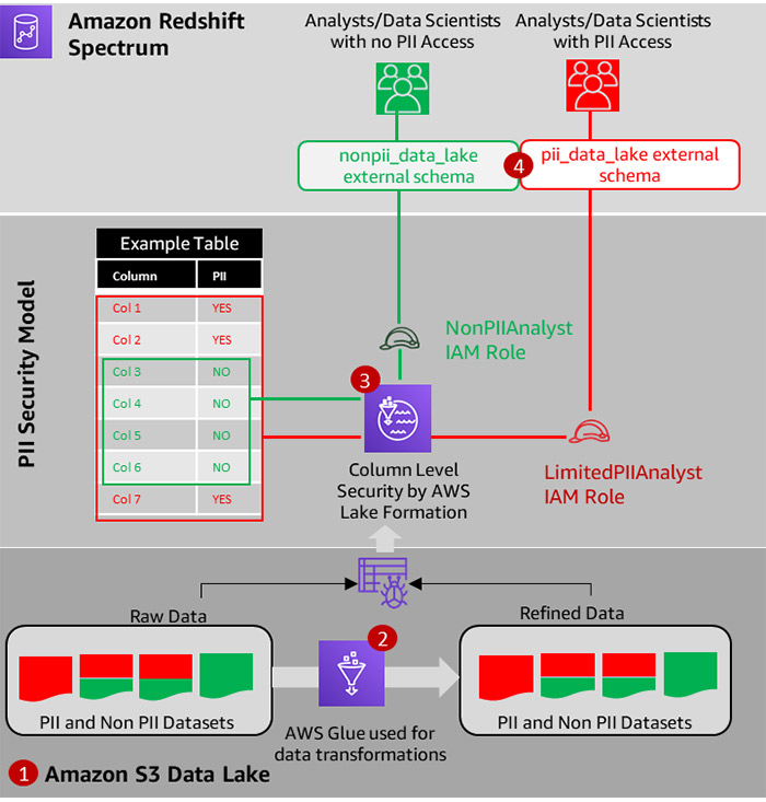
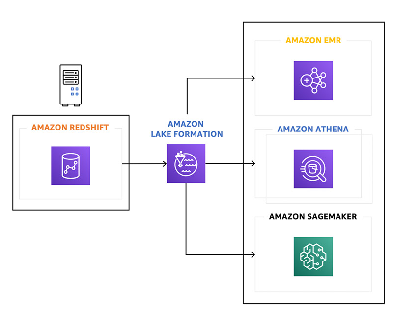
FanDuel decided to use Lake Formation and Redshift Spectrum to solve this challenge. The following architectural diagram shows how FanDuel secured their data lake.

The solution includes the following steps:

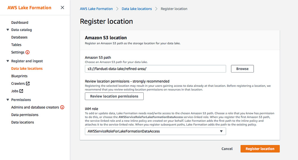
  1. The FanDuel team registered the S3 location in Lake Formation.

After the location is registered, Lake Formation takes control of the data lake, thereby eliminating the need to set up complicated policies in IAM.

  1. FanDuel built AWS Glue ETL jobs to extract data from sources, including MySQL databases and flat files. They used AWS Glue to cleanse and transform raw data to form refined datasets stored in Parquet-formatted files. They also used AWS Glue crawlers to register the cleansed datasets in the Data Catalog.
  2. The team used Lake Formation to set up column-based permissions using two roles:
    1. LimitedPIIAnalyst – Granted access to all columns. Only analysts who needed access to PII data were assigned this role.
    2. NonPIIAnalyst – Granted access to non-PII columns. By default, analysts using the data lake were assigned this role.
  3. FanDuel created two external schemas using Redshift Spectrum: one using the NonPIIAnalyst role, and one using the LimitedPIIAnalyst The following code is an example of the DDL that uses the role that was set up in Lake Formation:
    CREATE EXTERNAL SCHEMA nonpii_data_lake FROM DATA CATALOG
    DATABASE 'fanduel_data_lake' REGION 'us-east-1'
    IAM_ROLE 'arn:aws:iam::123456789012:role/NonPIIAnalyst';
    
    CREATE EXTERNAL SCHEMA limitedpii_data_lake FROM DATA CATALOG
    DATABASE 'fanduel_data_lake' REGION 'us-east-1'
    IAM_ROLE 'arn:aws:iam::123456789012:role/LimitedPIIAnalyst';
    

FanDuel could already manage access permissions by adding or removing users from a group in Amazon Redshift, so they already had a group consisting of only the analysts who should be permitted access to PII. The following code grants this group access to the limitedpii_data_lake schema, which effectively means only this group can query the data lake using the LimitedPIIAnalyst role:

GRANT USAGE ON SCHEMA nonpii_data_lake TO base_group;
GRANT SELECT ON ALL TABLES IN SCHEMA nonpii_data_lake TO base_group;
GRANT USAGE ON SCHEMA limitedpii_data_lake TO pii_permitted_group;
GRANT SELECT ON ALL TABLES IN SCHEMA limitedpii_data_lake TO pii_permitted_group;

Benefits

The ability to extend queries to the data lake with Redshift Spectrum and have column-level access control provides superior control over the S3 tag-based permissions approach that was originally considered. This architecture provided the following benefits for FanDuel:

  • FanDuel could offer new capabilities to data analysts. For example, data analysts could quickly access raw data with PII and combine it with existing data in Amazon Redshift. Lake Formation provided a single view for monitoring the data access patterns.
  • Lake Formation column-level access control allowed them to secure PII data, which otherwise would have taken a complex S3 tag-based approach. This saved 100–200 hours of development time for every new data source and data footprint, because the original approach required creating two files (one with PII and another without PII), tagging files, and setting up permissions based on tags.
  • The ability to extend access from Amazon Redshift to the data lake with appropriate access control has allowed FanDuel to reduce data stored in Amazon Redshift.

Conclusion

FanDuel will leverage its new data platform to ingest additional data sources with real-time data so analysts and data scientists can gain insights and improve customer experience.

Questions or feedback? Send an email to [email protected].


About the Authors

Damian Grech is a Data Engineering Senior Manager at FanDuel. Damian has over 15 years of experience in software delivery and has worked with organizations ranging from large enterprises to start-ups at their infant stages. In his spare time, you can find him either experimenting in the kitchen or trailing the Scottish Highlands.


Shiv Narayanan is Global Business Development Manager for Data Lakes and Analytics solutions at AWS. He works with AWS customers across the globe to strategize, build, develop and deploy modern data platforms. Shiv loves music, travel, food and trying out new tech.


Sidhanth Muralidhar is a Senior Technical Account Manager at Amazon Web Services. He works with large enterprise customers who run their workloads on AWS. He is passionate about working with customers and helping them in their cloud journey. In his spare time, he loves to play and watch football.


Sharing Amazon Redshift data securely across Amazon Redshift clusters for workload isolation

Post Syndicated from Harsha Tadiparthi original https://aws.amazon.com/blogs/big-data/sharing-amazon-redshift-data-securely-across-amazon-redshift-clusters-for-workload-isolation/

Amazon Redshift data sharing allows for a secure and easy way to share live data for read purposes across Amazon Redshift clusters. Amazon Redshift is a fast, fully managed cloud data warehouse that makes it simple and cost-effective to analyze all your data using standard SQL and your existing business intelligence (BI) tools. It allows you to run complex analytic queries against terabytes to petabytes of structured data, using sophisticated query optimization, columnar storage on high-performance storage, and massively parallel query runs.

In this post, we discuss how to use Amazon Redshift data sharing to achieve workload isolation across diverse analytics use cases and achieve business-critical SLAs. For more information about this new feature, see Announcing Amazon Redshift data sharing (preview).

How to use Amazon Redshift data sharing

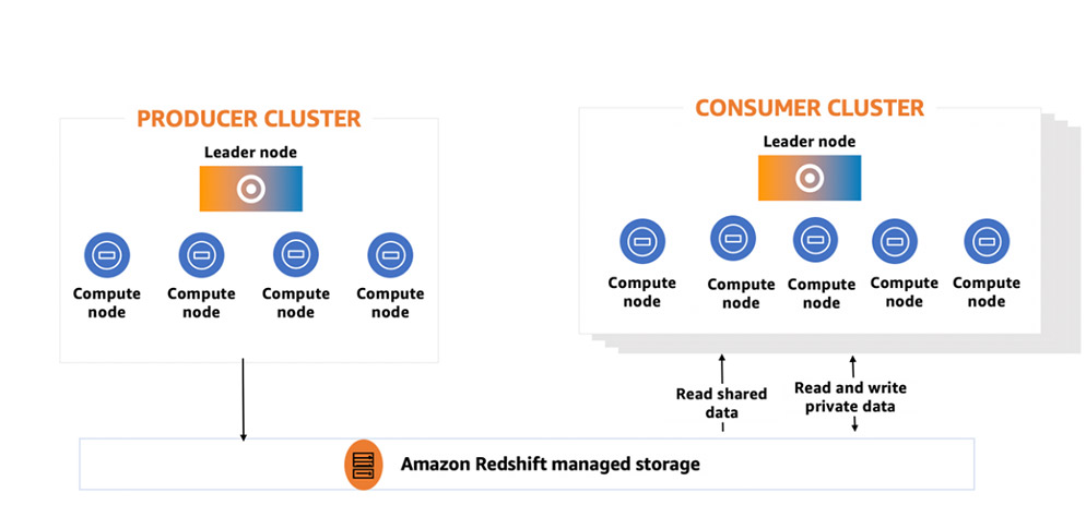
Amazon Redshift data sharing allows a producer cluster to share data objects to one or more Amazon Redshift consumer clusters for read purposes without having to copy the data. With this approach, workloads isolated to different clusters can share and collaborate frequently on data to drive innovation and offer value-added analytic services to your internal and external stakeholders. You can share data at many levels, including databases, schemas, tables, views, columns, and user-defined functions, to provide fine-grained access controls that can be tailored for different users and businesses that all need access to Amazon Redshift data.

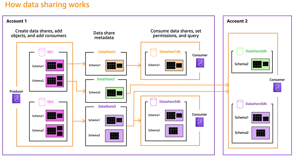
Data sharing between Amazon Redshift clusters is a two-step process. First, the producer cluster administrator that wants to share data creates an Amazon Redshift data share, a new named object introduced with this release to serve as a unit of sharing. The producer cluster adds the needed database objects such as schemas, tables, and views to the data share and specifies a list of consumer clusters with which to share the data share. Following that, privileged users on consumer clusters create an Amazon Redshift local database reference from the data share made available to them and grant permissions on the database objects to appropriate users and groups. Users and groups can then list the shared objects as part of the standard metadata queries and start querying immediately.

Solution overview

For this post, we use a use case in which the producer cluster is a central ETL cluster hosting enterprise sales data, a 3 TB Cloud DW benchmark dataset based on the TPC-DS benchmark dataset. This cluster serves multiple BI and data science clusters purpose-built for distinct business groups within the organization. One such group is the sales BI team, who runs BI reports using customer sales data created in the central ETL cluster and joined with the product reviews dataset that they loaded into the BI cluster they manage.

This approach helps the sales BI team isolate data lifecycle management between the enterprise sales dataset in the ETL producer from the product reviews data that they fully manage in the BI consumer cluster to simplify data stewardship. It also allows for agility, allows sizing clusters independently to provide workload isolation, and creates a simple cost charge-back model.

As depicted in the following diagram, the central ETL cluster etl_cluster hosts the sales data in a schema named sales. We demonstrate how to build the semantic layer later in this post. A superuser in etl_cluster then creates a data share named salesdatashare, adds the bi_semantic schema and all objects in that schema to the data share, and grants usage permissions to the BI consumer cluster named bi_cluster. Keep in mind that a data share is simply a metadata container and represents what data is shared from producer to consumer. No data is actually moved.

As depicted in the following diagram, the central ETL cluster etl_cluster hosts the sales data in a schema named sales and performs transformations to create a semantic layer required for BI reports in a new schema named bi_semantic.

The superuser in the BI consumer cluster creates a local database reference named sales_semantic from the data share (step 2 in the preceding diagram). The BI users use the product reviews dataset in the local schema named product_reviews and join with bi_semantic data for reporting purposes (step 3).

You can find the script in the products review dataset, which we use in this post to load the dataset into bi_cluster. You can load the DW benchmark dataset into etl_cluster using this github link. Loading these datasets into the respective Amazon Redshift clusters is outside the scope of this post, and is a prerequisite to following the instructions we outline.

The following diagram depicts the cloud DW benchmark data model used.

The following diagram depicts the cloud DW benchmark data model used.

The following table summarizes the data.

Table Name Rows
STORE_SALES 8,639,936,081
CUSTOMER_ADDRESS 15,000,000
CUSTOMER 30,000,000
CUSTOMER_DEMOGRAPHICS 1,920,800
ITEM 360,000
DATE_DIM 73,049

Building a BI semantic layer

A BI semantic layer is a representation of enterprise data in a way that simplifies BI reporting requirements and offers better performance. In our use case, the BI semantic layer transforms sales data to create a customer denormalized dataset and another dataset for all store sales by product in a given year. The following queries are run on the etl_cluster to create the BI semantic layer.

  1. Create a new schema to host BI semantic tables with the following SQL:
    Create schema bi_semantic;

  2. Create a denormalized customer view with select columns required for sales BI team:
    create view bi_semantic.customer_denorm 
    as
    select
    	c_customer_sk,
    	c_customer_id,
    	c_birth_year,
    	c_birth_country,
    	c_last_review_date_sk,
    	ca_city,
    	ca_state,
    	ca_zip,
    	ca_country,
    	ca_gmt_offset,
    	cd_gender,
    	cd_marital_status,
    	cd_education_status
    from sales.customer c, sales.customer_address ca, sales.customer_demographics cd
    where
    c.c_current_addr_sk=ca.ca_address_sk
    and c.c_current_cdemo_sk=cd.cd_demo_sk;

  1. Create a second view for all product sales with columns required for BI team:
    create view bi_semantic.product_sales
    as 
    select 
    	i_item_id,
    	i_product_name,
    	i_current_price,
    	i_wholesale_cost,
    	i_brand_id,
    	i_brand,
    	i_category_id,
    	i_category,
    	i_manufact,
    	d_date,
    	d_moy,
    	d_year,
    	d_quarter_name,
    	ss_customer_sk,
    	ss_store_sk,
    	ss_sales_price,
    	ss_list_price,
    	ss_net_profit,
    	ss_quantity,
    	ss_coupon_amt
    from sales.store_sales ss, sales.item i, sales.date_dim d
    where ss.ss_item_sk=i.i_item_sk
    and ss.ss_sold_date_sk=d.d_date_sk;

Sharing data across Amazon Redshift clusters

Now, let’s share the bi_semantic schema in the etl_cluster with the bi _cluster.

  1. Create a data share in the etl_cluster using the following command when connected to the etl_cluster. The producer cluster superuser and database owners can create data share objects. By default, PUBLICACCESSIBLE is false. If the producer cluster is publicly accessible, you can add PUBLICACCESSIBLE = true to the following command:
    CREATE DATASHARE SalesDatashare;

  1. Add the BI semantic views to the data share. To add objects to the data share, add the schema before adding objects. Use ALTER DATASHARE to share the entire schema; to share tables, views, and functions in a given schema; and to share objects from multiple schemas:
    ALTER DATASHARE SalesDatashare ADD SCHEMA bi_semantic;
    ALTER DATASHARE SalesDatashare ADD ALL TABLES IN SCHEMA bi_semantic;

The next step requires a cluster namespace GUID from the bi_cluster. One way to find the namespace value of a cluster is to run the SQL statement select current_namespace when connected to the bi_cluster. Another way is on the Amazon Redshift console: choose your Amazon Redshift consumer cluster, and find the value under Namespace located in the General information section.

  1. Add consumers to the data share using the following command:
    GRANT USAGE ON DATASHARE SalesDatashare TO NAMESPACE '1m137c4-1187-4bf3-8ce2-e710b7100eb2';

  1. View the list of the objects added to the share using the following command. The share type is outbound on the producer cluster.
    DESC DATASHARE salesdatashare;

The following screenshot shows our list of objects.

The following screenshot shows our list of objects.

Consuming the data share from the consumer BI Amazon Redshift cluster

From the bi_cluster, let’s review, consume, and set permissions on the data share for end-user consumption.

  1. On the consumer BI cluster, view the data shares using the following command as any user:
    SHOW DATASHARES;

The following screenshot shows our results. Consumers should be able to see the objects within the incoming share but not the full list of consumers associated with the share. For more information about querying the metadata of shares, see DESC DATASHARE.

The following screenshot shows our results.

  1. Start the consumption by creating a local database from the salesdatashare. Cluster users with the permission to do so can create a database from the shares. We use the namespace from the etl_cluster.
    CREATE DATABASE Sales_semantic from DATASHARE SalesDatashare OF NAMESPACE '45b137c4-1287-4vf3-8cw2-e710b7138nd9'; 

Consumers should be able to see databases that they created from the share, along with the databases local to the cluster, at any point by querying SVV_REDSHIFT* tables. Data share objects aren’t available for queries until a local database reference is created using a create database statement.

  1. Run the following command to list the databases in bi_cluster:
    select * from svv_redshift_databases;

The following screenshot shows that both the local and shared databases are listed so that you can explore and navigate metadata for shared datasets.

The following screenshot shows that both the local and shared databases are listed so that you can explore and navigate metadata for shared datasets.

  1. Grant usage on the database to bi_group, where bi_group is a local Amazon Redshift group with BI users added to that group:
    GRANT USAGE ON DATABASE sales_semantic TO bi_group;

Querying as the BI user

In this section, you connect as a user in the bi_group who got access to the shared data. The user is still connected to the local database on the bi_cluster but can query the shared data via the new cross-database query functionality in Amazon Redshift.

  1. Review the list of objects in the share by running the following SQL:
    SELECT schema_name, table_name, table_type FROM  svv_redshift_tables
         where database_name = 'sales_semantic'

The following screenshot shows our results.

The following screenshot shows our results.

  1. Review the list of columns in the customer_denorm view::
    SELECT * FROM  svv_redshift_columns 
       where database_name = 'sales_semantic' and table_name = 'customer_denorm';

The following screenshot shows our results.

The following screenshot shows our results.

  1. Query the shared objects using three-part notation just like querying any other local database object, using a notation <database>.<schema>.<view/table>:
    select count(*) from sales_semantic.bi_semantic.customer_denorm;

Following is your result:

28950139

  1. Analyze the local product reviews data by joining the shared customer_denorm data to identify the top ratings by customer states for this BI report:
    SELECT PR.product_category, c.ca_state AS customer_state,
                  count(PR.star_rating) AS cnt
          FROM product_reviews.amazon_reviews PR,               --local data
               sales_semantic.bi_semantic.customer_denorm  C    –-shared data
          WHERE  PR.customer_id = C.c_customer_sk
             AND PR.marketplace = 'US'
          GROUP BY 1, 2
          order by cnt desc
          Limit 10;

The following screenshot shows our results.

The following screenshot shows our results.

Adding a data science consumer

Now, let’s assume the company has decided to spin up a data science team to help with new sales strategies, and this team performs analytics on the sales data. The data science team is new and has very different access patterns and SLA requirements compared to the BI team. Thanks to the data sharing feature, onboarding new use cases such as this is easy.

We add a data science consumer cluster named ds_cluster. Because the data science users need access to data in salesdatashare, the superuser in the etl_cluster can simply grant access to the ds_cluster by adding them as another consumer for the share without moving any data:

GRANT USAGE ON DATASHARE SalesDatashare TO NAMESPACE ''1h137c4-1187-4w53-8de2-e710b7100es2';

The following diagram shows our updated architecture with the data science consumer (step 4).

The following diagram shows our updated architecture with the data science consumer (step 4).

This way, multiple clusters of different sizes can access the same dataset and isolate workloads to meet their SLA requirements. Users in these respective clusters are granted access to shared objects to meet their stringent security requirements. The producer keeps control of the data and at any point can remove certain objects from the share or remove access to the share for any of these clusters, and the consumers immediately lose access to the data. Also, as more data is ingested into the producer cluster, the consumer sees transactionally consistent data instantly.

Monitoring and security

Amazon Redshift offers comprehensive auditing capabilities using system tables and AWS CloudTrail to allow you to monitor the data sharing permissions and usage across all the consumers and revoke access instantly when necessary. The permissions are granted by the superusers from both the producer and the consumer clusters to define who gets access to what objects, similar to the grant commands used in the earlier scenario. You can use the following commands to audit the usage and activities for the data share.

Track all changes to the data share and the shared database imported from the data share with the following code:

Select username, share_name, recordtime, action, 
         share_object_type, share_object_name 
  from svl_datashare_change_log
   order by recordtime desc;

The following screenshot shows our results.

The following screenshot shows our results.

Track data share access activity (usage), which is relevant only on the producer, with the following code:

Select * from svl_datashare_usage;

The following screenshot shows our results.

The following screenshot shows our results.

Summary

Amazon Redshift data sharing provides workload isolation by allowing multiple consumers to share data seamlessly without the need to unload and load data. We also presented a step-by-step guide for securely sharing data from a producer to multiple consumer clusters.


About the Authors

Harsha Tadiparthi is a Specialist Sr. Solutions Architect, AWS Analytics. He enjoys solving complex customer problems in Databases and Analytics and delivering successful outcomes. Outside of work, he loves to spend time with his family, watch movies, and travel whenever possible.


Harshida Patel is a Specialist Sr. Solutions Architect, Analytics with AWS.

Announcing Amazon Redshift federated querying to Amazon Aurora MySQL and Amazon RDS for MySQL

Post Syndicated from BP Yau original https://aws.amazon.com/blogs/big-data/announcing-amazon-redshift-federated-querying-to-amazon-aurora-mysql-and-amazon-rds-for-mysql/

Since we launched Amazon Redshift as a cloud data warehouse service more than seven years ago, tens of thousands of customers have built analytics workloads using it. We’re always listening to your feedback and, in April 2020, we announced general availability for federated querying to Amazon Aurora PostgreSQL and Amazon Relational Database Service (Amazon RDS) for PostgreSQL to enable you to query data across your operational databases, your data warehouse, and your data lake to gain faster and deeper insights not possible otherwise.

Today, we’re launching a new feature of Amazon Redshift federated query to Amazon Aurora MySQL and Amazon RDS for MySQL to help you expand your operational databases in the MySQL family. With this lake house architecture expansion to support more operational data stores, you can query and combine data more easily in real time and store data in open file formats in your Amazon Simple Storage Service (Amazon S3) data lake. Your data can then be more available to other analytics and machine learning (ML) tools, rather than siloed in disparate data stores.

In this post, we share information about how to get started with this new federated query feature to MySQL.

Prerequisites

To try this new feature, create a new Amazon Redshift cluster in a sql_preview maintenance track and Aurora MySQL instance and load sample TPC data into both data stores. To make sure both Aurora MySQL DB instances can accept connections from the Amazon Redshift cluster, you should make sure that both your Amazon Redshift cluster and Aurora MySQL instances are in the same Amazon Virtual Private Cloud (Amazon VPC) and subnet group. This way, you can add the security group for the Amazon Redshift cluster to the inbound rules of the security group for the Aurora MySQL DB instance.

If your Amazon Redshift cluster and Aurora MySQL instances are in the different VPC, you can set up VPC peering or other networking to allow Amazon Redshift to make connections to your Aurora MySQL instances. For more information about VPC networking, see Working with a DB instance in a VPC.

Configuring AWS Secrets Manager for remote database credentials

Amazon Redshift needs database credentials to issue a federated query to a MySQL database. AWS Secrets Manager provides a centralized service to manage secrets and can be used to store your MySQL database credentials. Because Amazon Redshift retrieves and uses these credentials, they are transient, not stored in any generated code, and discarded after the query runs.

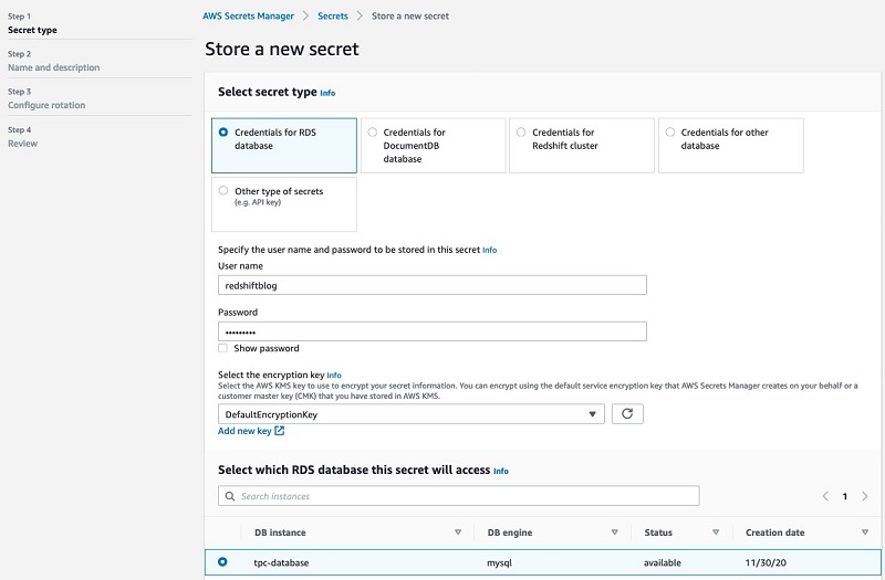
Storing credentials in Secrets Manager takes only a few minutes. To store a new secret, complete the following steps:

  1. On the Secrets Manager console, choose Secrets.
  2. Choose Store a new secret.
  3. For Select secret type, select Credentials for RDS database.
  4. For User name, enter a name.
  5. For Password, enter a password.
  6. For Select the encryption key, choose DefaultEncryptionkey.
  7. For Select which RDS database this secret will access, choose your database.

Storing credentials in Secrets Manager takes only a few minutes.

  1. Optionally, copy programmatic code for accessing your secret using your preferred programming languages (which is not needed for this post).
  2. Choose Next.

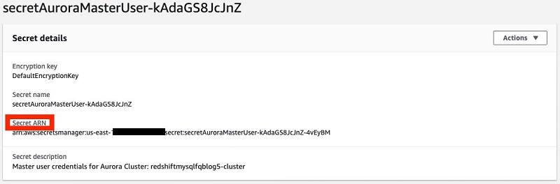
After you create the secret, you can retrieve the secret ARN by choosing the secret on the Secrets Manager console. The secret ARN is needed in the subsequent step.

After you create the secret, you can retrieve the secret ARN by choosing the secret on the Secrets Manager console.

Setting up IAM role

You can now pull everything together by embedding the secret ARN into an AWS Identity and Access Management (IAM) policy, naming the policy, and attaching it to an IAM role. See the following code:

{
    "Version": "2012-10-17",
    "Statement": [
        {
            "Sid": "AccessSecret",
            "Effect": "Allow",
            "Action": [
                "secretsmanager:GetResourcePolicy",
                "secretsmanager:GetSecretValue",
                "secretsmanager:DescribeSecret",
                "secretsmanager:ListSecretVersionIds"
            ],
            "Resource": "<SecretARN>"
        },
        {
            "Sid": "VisualEditor1",
            "Effect": "Allow",
            "Action": [
                "secretsmanager:GetRandomPassword",
                "secretsmanager:ListSecrets"
            ],
            "Resource": "*"
        }
    ]
}

Finally, attach the same IAM role to your Amazon Redshift cluster.

  1. On the Amazon Redshift console, choose Clusters.
  2. Choose your cluster.
  3. On the Actions drop-down menu, choose Manage IAM roles.

Finally, attach the same IAM role to your Amazon Redshift cluster.

  1. Choose and add the IAM role you just created.

Setting up external schema

The final step is to create an external schema to connect to your Aurora MySQL instance. The following example code creates the external schema statement that you need to run on your Amazon Redshift cluster to complete this step:

CREATE EXTERNAL SCHEMA IF NOT EXISTS mysqlfq 
FROM MYSQL 
DATABASE 'tpc' 
URI '<AuroraClusterEndpoint>' 
PORT 3306 
IAM_ROLE '<IAMRole>' 
SECRET_ARN '<SecretARN>'

Use the following parameters:

  • URI – Aurora MySQL cluster endpoint
  • IAM_Role – IAM role created from the previous step
  • Secret_ARN – Secret ARN

After you set up the external schema, you’re ready to run some queries to test different use cases.

Querying live operational data

You can now query real-time operational data in your Aurora MySQL instance from Amazon Redshift. Note that isolation level is read committed for MySQL. See the following code:

dev=# select top 10 ws_order_number from mysqlfq.web_sales;
 ws_order_number 
-----------------
        93628990
       157020207
         4338647
        41395871
        58468186
       171095867
        12514566
        74946143
         3418243
        67054239
(10 rows)

Querying mysqlfq.web_sales in Amazon Redshift routes the request to MySQL tpc database and web_sales table. If you examine the query plan, you can see the query runs at the MySQL instance as shown by the step Remote MySQL Seq Scan:

dev=# explain select top 10 ws_order_number from mysqlfq.web_sales;
                                          QUERY PLAN                                           
-----------------------------------------------------------------------------------------------
 XN Limit  (cost=0.00..0.20 rows=10 width=8)
   ->  XN MySQL Query Scan web_sales  (cost=0.00..6869.28 rows=343464 width=8)
         ->  Remote MySQL Seq Scan mysqlfq.web_sales  (cost=0.00..3434.64 rows=343464 width=8)
(3 rows)

Simplifying ELT and ETL

You can also extract operational data directly from your Aurora MySQL instance and load it into Amazon Redshift. See the following code:

dev=# create table staging_customer as select c_customer_id from mysqlfq.customer where c_customer_id not in (select c_customer_id from customer);
SELECT
dev=# select count(*) from staging_customer;
 count  
--------
 350000
(1 row)

The preceding code uses CTAS to create and load incremental data from your operational MySQL instance into a staging table in Amazon Redshift. You can then perform transformation and merge operations from the staging table to the target table. For more information, see Updating and inserting new data.

Combining operational data with data from your data warehouse and data lake

You can combine live operational data from your Aurora MySQL instance with data from your Amazon Redshift data warehouse and S3 data lake by creating a late binding view.

To access your S3 data lake historical data via Amazon Redshift Spectrum, create an external table:

create external schema mysqlspectrum
from data catalog
database 'spectrumdb'
iam_role '<IAMRole>'
create external database if not exists;
 
create external table mysqlspectrum.customer 
stored as parquet 
location 's3://<yourS3bucket>/customer/'
as select * from customer where c_customer_sk <= 100000;

You can then run queries on the view to gain insight on data across the three sources:

drop view vwCustomer;
create view vwCustomer as
select c_customer_sk, 'redshift' as source from public.customer where c_customer_sk > 100000
union all
select c_customer_sk, 'mysql' as source from mysqlfq.customer
union all
select c_customer_sk, 's3' as source from mysqlspectrum.customer
with no schema binding;

select * from vwCustomer where c_customer_sk in (1, 149712,29033279);

You should the following three records as output:

dev=# select * from vwCustomer where c_customer_sk in (1, 149712,29033279);
 c_customer_sk |  source  
---------------+----------
      29033279 | mysql
             1 | s3
        149712 | redshift
(3 rows)

If you examine the query plan, you can see that the predicates are pushed down to your MySQL instance to run:

dev=# explain select * from vwCustomer where c_customer_sk in (1,149712,29033279);
                                                                            QUERY PLAN                                                                            
------------------------------------------------------------------------------------------------------------------------------------------------------------------
 XN Subquery Scan vwcustomer  (cost=0.00..48398.40 rows=6988 width=36)
   ->  XN Append  (cost=0.00..48328.52 rows=6988 width=4)
         ->  XN Subquery Scan "*SELECT* 1"  (cost=0.00..40000.03 rows=3 width=4)
               ->  XN Seq Scan on customer  (cost=0.00..40000.00 rows=3 width=4)
                     Filter: (((c_customer_sk = 1) OR (c_customer_sk = 149712) OR (c_customer_sk = 29033279)) AND (c_customer_sk > 100000))
         ->  XN Subquery Scan "*SELECT* 2"  (cost=0.00..6548.63 rows=5492 width=4)
               ->  XN MySQL Query Scan customer  (cost=0.00..6493.71 rows=5492 width=4)
                     ->  Remote MySQL Seq Scan mysqlfq.customer  (cost=0.00..6438.79 rows=5492 width=4)
                           Filter: ((c_customer_sk = 1) OR (c_customer_sk = 149712) OR (c_customer_sk = 29033279))
         ->  XN Subquery Scan "*SELECT* 3"  (cost=0.00..1779.86 rows=1493 width=4)
               ->  XN S3 Query Scan customer  (cost=0.00..1764.93 rows=1493 width=4)
                     ->  S3 Seq Scan mysqlspectrum.customer location:"s3://<yourS3bucket>/customer" format:PARQUET  (cost=0.00..1750.00 rows=1493 width=4)
                           Filter: ((c_customer_sk = 1) OR (c_customer_sk = 149712) OR (c_customer_sk = 29033279))
(13 rows)

Available Now

Amazon Redshift federated querying to Aurora MySQL and Amazon RDS for MySQL is now available for public preview with Amazon Redshift release version 1.0.21591 or later. Refer to the AWS Region Table for Amazon Redshift availability and to check the version of your clusters.


About the Authors

BP Yau is an Analytics Specialist Solutions Architect at AWS. His role is to help customers architect big data solutions to process data at scale. Before AWS, he helped Amazon.com Supply Chain Optimization Technologies migrate its Oracle data warehouse to Amazon Redshift and build its next-generation big data analytics platform using AWS technologies.


Zhouyi Yang is a Software Development Engineer for the Amazon Redshift Query Processing team. He’s passionate about gaining new knowledge about large databases and has worked on SQL language features such as federated query and IAM role privilege control. In his spare time, he enjoys swimming, tennis, and reading.


Entong Shen is a Senior Software Development Engineer for Amazon Redshift. He has been working on MPP databases for over 8 years and has focused on query optimization, statistics, and SQL language features such as stored procedures and federated query. In his spare time, he enjoys listening to music of all genres and working in his succulent garden.

Building high-quality benchmark tests for Amazon Redshift using SQLWorkbench and psql

Post Syndicated from Asser Moustafa original https://aws.amazon.com/blogs/big-data/building-high-quality-benchmark-tests-for-amazon-redshift-using-sqlworkbench-and-psql/

In the introductory post of this series, we discussed benchmarking benefits and best practices common across different open-source benchmarking tools. In this post, we discuss benchmarking Amazon Redshift with the SQLWorkbench and psql open-source tools. Let’s first start with a quick review of the introductory installment.

When you use Amazon Redshift to scale compute and storage independently, a need arises to profile the compute requirements of various production workloads so that your Amazon Redshift cluster configuration reflects an appropriately balanced compute layer. You also need an approach to scale up with eyes wide open, and benchmarking different Amazon Redshift cluster configurations against various production workloads can help you appropriately accommodate workload expansion. In addition, you may also use benchmark tests to proactively monitor a production cluster’s performance in real time.

For prospective Amazon Redshift customers, benchmarking Amazon Redshift is often one of the main components of their evaluation and a key source of insight into the price-to-performance ratio of different Amazon Redshift configurations.

Open-source tools, with their cost-efficiency and vendor neutrality, are often the preferred choice for profiling production workloads and benchmark tests. However, best practices for using these tools are scarce, possibly resulting in flawed compute profiles, flawed benchmark results, customer frustration, and bloated timelines.

One final point before we get started: there is a lot that could be said about benchmarking—more than can be accommodated in a single post. Analytics Specialists Solutions Architects such as myself frequently and happily engage with current and prospective customers to help you evaluate your benchmarking strategy and approach at no charge. I highly recommend you take advantage of that benefit by reaching out to your AWS account Solutions Architect.

SQLWorkbench

SQLWorkbench, also referred to as SQLWorkbench/J, is an open-source SQL query tool that you can freely download as a .zip file. It’s written in Java so it runs on Windows, Linux/UNIX, and macOS, and naturally requires a supported Java runtime environment (JRE). SQLWorkbench also requires a JDBC driver for the database (to download the latest Amazon Redshift JDBC driver, see Configuring a JDBC driver version 1.0 connection).

SQLWorkbench can run in GUI or console mode. I discuss both in this section, but in my experience, customers typically default to the GUI mode, so we explore that version first. Also, I have found that customers that use SQLWorkbench often use it in a Windows environment (something to keep in mind if operating system has a determination on which open-source tool you use).

Typically, you stand up a Windows EC2 instance to serve as your benchmark host, and install SQLWorkbench on that machine. When you have SQLWorkbench running, setting up a connection to your Amazon Redshift cluster is quite easy. For this post, I assume you’re familiar with the basics of JDBC connections. The following screenshot shows what the SQLWorkbench connection dialog box might look like when populated with connection information.

After establishing a successful connection to your Amazon Redshift cluster, a query tab opens, in which you can write and run SQL queries similar to that shown in the following screenshot.

For benchmark tests, it’s highly recommended to set the maxrows field to a relatively low number to avoid noise from long transmission times of large result sets.

Unlike the LIMIT clause in a SQL SELECT statement, which can alter (short-circuit) Amazon Redshift query processing, setting the maxrows field (whether to a value as low as 1 or something much higher) has no impact on query processing in Amazon Redshift; maxrows only impacts SQLWorkbench’s rendering workload and overhead. You can easily verify this by running the same query multiple times with different maxrows settings and observing that the number of rows returned for each query on the Amazon Redshift console query history page doesn’t change. Although the resulting query times should still be considered as query runtimes, they certainly help you get closer to a query’s execution time. Setting the maxrows field to a relatively low number also reduces the risk of SQLWorkbench running into an out-of-memory error from very large result sets.

This straightforward GUI interface is appealing because it has a minimal learning curve and quickly enables you to start submitting benchmark tests against your Amazon Redshift cluster. SQLWorkbench is a very useful tool, and it may be a good fit for informal or simple benchmark tests that deal with a handful of benchmark queries, relatively small tables (such as under 50 million rows in a fact table), and are focused more on determining general directionality of query runtimes (for example, cluster A was faster than cluster B at running business query 123), rather than capturing accurate query runtimes. The GUI interface can also be helpful for quickly and easily tweaking test queries to be more or less intense, or to correct SQL syntax if the query originated from a different platform.

However, for more formal and complex benchmark tests that deal with large tables and must capture accurate query runtimes, SQLWorkbench’s straightforward GUI interface faces a scalability challenge: inputting potentially hundreds or thousands of benchmark queries, running them sequentially or simultaneously, and capturing their runtimes in a practical manner can prove to be a huge challenge.

In addition, SQLWorkBench’s rendering and processing times for query result sets are added to a query’s runtime, and so even moderately sized query result sets can lead to potentially significant noise in query runtimes. For example, I recently observed a customer reduce their query runtimes by several orders of magnitude by switching to a command line tool while keeping all other aspects of their benchmark tests and environment constant. Some of the queries were straightforward filter queries with no joins, returning 400,000 rows from a 2 billion-row fact table with approximately 30 mostly integer columns.

Using console mode

One way to minimize the scale problem and rendering noise is to switch to SQLWorkbench console mode (the command line interface), which comes bundled with the GUI version of SQLWorkbench in the same downloadable .zip file.

In this section, we show one way to enter console mode from the Windows command line prompt (note the -showTiming=true flag that enables query execution times print on the screen) and connect to an Amazon Redshift cluster.

The following code starts SQLWorkbench in console mode:

c:\ sqlwbconsole64.exe -showTiming=true

When you’re in console mode, use the following command to connect to an Amazon Redshift cluster:

SQL> WbConnect -username=<Redshift User> -password=<Redshift User Password> -url=<fully qualified Redshift JDBC URL with port and database> -driver=<Redshift JDBC driver class name>
For example:
SQL> WbConnect -username=demouser -password=******* -url=jdbc:redshift://demo-poc-redshift-cluster.xxxxxx.us-west-2.redshift.amazonaws.com:8192/dev -driver=com.amazon.redshift.jdbc.Driver

The following screenshot shows our output.

Again, it’s recommended to set the maximum rows for the results sets to a relatively low number, using the following command:

SQL> set maxrows <number>;

Although console mode may have a slightly higher learning curve, it can significantly reduce potential rendering noise in a query’s runtime. In addition, SQLWorkbench’s console mode lends itself to scripting, which opens the door to many more sophisticated benchmarking scenarios, particularly when simulating concurrent users and capturing sophisticated metrics.

Comparing performance of SQLWorkbench modes

Let’s use an example use case to demonstrate the potential performance differences of both modes of SQLWorkbench. Although Example Corp is a hypothetical company, the use case is quite typical and realistic, and the benchmark results presented are based on actual customer experiences.

Example Corp has onboarded terabytes of data, over 100 ETL jobs, and thousands of business users to our Amazon Redshift deployment over the past quarter. Data architects and engineers have observed the Amazon Redshift cluster’s average CPU utilization steadily increase, and now wish to scale up the cluster before onboarding additional data, ETL jobs, and users waiting in the project pipeline.

To determine the optimal cluster size, we perform a few simple benchmark tests on different cluster configurations. We first identify five or so sufficiently complex production queries for benchmarking clusters of different sizes and instance types. We decide query runtime is a sufficient measure of the optimal cluster size, because we’re mainly interested in directional guidance (for example, query runtimes improved significantly with 1.5x cluster size, but only marginally with larger than 1.5x cluster sizes).

We can use an Amazon Redshift snapshot from our production cluster to quickly stand up a few differently configured clusters varying in node size or node type (such as ra3.4xl vs. ra3.16xl). We use a production snapshot to create the benchmark clusters so we can keep the cluster data identical.

However, manually running the benchmark queries individually using the SQLWorkbench GUI shows query runtimes actually increased in most cases (compared to the original production cluster) despite the more powerful clusters! Upon a closer look, we realize internet transport noise has not been isolated from the query runtimes. We stand up a dedicated test EC2 machine in the same VPC and Availability Zone as our benchmark Amazon Redshift clusters and install a SQLWorkbench GUI client.

Running the benchmark queries using the SQLWorkbench GUI provides similar query runtimes as the original cluster configuration. Again, not what was expected. Upon switching to SQLWorkbench console mode, however, we observe an improvement in query runtimes by several orders of magnitude.

psql

In my experience, psql is the preferred open-source command line query tool for customers running in a Linux/UNIX environment, so in this post, I assume a Linux EC2 instance is being used to run psql. If the standard Amazon Linux AMI was chosen (usually the first one in the list) during EC2 creation, you can use the following commands to update and verify psql v9.2 on the Linux EC2 instance:

> sudo yum update
> sudo yum install postgresql
> psql --help

Feel free to also search the freely available community AMIs, which might have newer versions of PostGreSQL server and the psql client pre-installed.

After psql is installed, connecting to an Amazon Redshift cluster is pretty straightforward by specifying a few command line parameters:

psql -h <Redshift JDBC endpoint> -p <Redshift port> -U <Redshift user> -d <Redshift database> 

The standard Amazon Redshift port is 5439, but I use port 8192 in the following code because of certain firewall requirements in my environment:

psql -h benchmark-redshift-cluster1.xxxxx.us-west-2.redshift.amazonaws.com -p 5439 -U masteruser -d dev

The following screenshot shows our output.

After you connect to the Amazon Redshift cluster, be sure to run the \timing on command to enable query timing.

It’s also highly recommended that you consider setting the FETCH_COUNT variable to a relatively low number on the psql console to avoid long transmission times for large result sets:

\set FETCH_COUNT 500 

By setting this variable, database cursors and the FETCH command are used in conjunction with queries. Setting this variable has no impact on query processing in Amazon Redshift, but rather the number of rows returned to the client application from the fully materialized result set.

Although the command line nature of psql may have a slightly higher learning curve than similar GUI applications, it also helps keep it lightweight and introduces minimal processing noise into a query’s runtime. For example, I observed a customer’s query runtime improve by several orders of magnitude by simply switching from a GUI tool to command line psql, while keeping all other aspects of the benchmark test and environment constant.

In addition, psql’s command line interface lends itself to scripting, which opens the door to many more sophisticated benchmarking scenarios, particularly when simulating concurrent users and capturing sophisticated concurrency metrics. In fact, a number of customizable, parameter-driven scripts have already been written by AWS Analytics Specialists such as myself for sophisticated benchmarking compute and concurrency scenarios, and are freely available to current and prospective customers.

Another utility that you can use in combination with such scripts is Simple Replay, a utility that is freely available on the Amazon Redshift Utilities GitHub repo. Simply Replay can extract workload histories from a source Amazon Redshift cluster and replay those workloads (using the psql command line client) with high fidelity on a different (such as a benchmark test) Amazon Redshift cluster.

For Simple Replay to extract workload details from an Amazon Redshift cluster, audit logging must be enabled in the cluster, and it may take about an hour for the most recent workloads to propagate to the audit logs.

After we run the extract command, Simple Replay extracts workload information such as the connection patterns (for example, number of users and their connection timing), COPY and UNLOAD commands, and other SQL queries so that they can be replayed on a different Amazon Redshift cluster with high fidelity (and, in our case, using psql command line as the SQL client). The following screenshot shows our output.

The workload details are typically stored in an Amazon Simple Storage Service (Amazon S3) bucket, which is specified in the Simple Replay configuration file, among other properties. See the following screenshot.

After running the python3 Extraction.py extraction.yaml command on the command line, we can review the workload details in our target S3 bucket to verify that the expected complexity was captured. The following screenshot shows the workload details on the Amazon S3 console.

The next step is to replay the extracted workload on a baseline cluster that mirrors our production cluster configuration (to establish a baseline runtime profile) and one or more target clusters using Simple Replay’s replay capability, as shown in the following screenshot.

Now let’s take another look at the example scenario presented in the previous section to demonstrate using the psql command line client with Simple Replay. Again, Example Corp has onboarded terabytes of data, over 100 ETL jobs, and thousands of business users to our Amazon Redshift deployment over the past quarter. Data architects and engineers have observed the Amazon Redshift cluster’s average CPU utilization steadily increase, and now wish to scale the cluster up (again) before onboarding additional data, ETL jobs, and users waiting in the project pipeline.

To determine the optimal cluster size, we first use the Simple Replay utility to extract information on all concurrent workloads that have occurred in the past 48 hours, from one-time user queries to BI reporting queries to ETL transformations. After we extract the information from the logs of the source Amazon Redshift cluster, we replay the same workloads on various benchmark cluster configurations. We may repeat this process for other timeframes in the past, such as month-end reporting or timeframes that exhibited unexpected workload spikes. To determine the optimal cluster size, the Example Corp team observes the CPU utilization of each benchmark cluster configuration and chooses the best cluster offering the best price-to-performance ratio.

For other capabilities and functionality in psql scripts, I recommend you reach out to your AWS account SA to evaluate available benchmarking scripts in relation to your needs and perhaps avoid “reinventing the wheel.”

Conclusion

In this series of posts, we discussed a number of recommended best practices for conducting high-quality benchmark tests. Some of the best practices represented core principles that span all the open-source tools discussed (such as consistency in testing methodology). In this post, we reviewed the strengths and appropriateness of SQLWorkbench and psql for conducting benchmark tests. I hope this series has been helpful, and strongly encourage current and prospective customers to reach out to me or other AWS colleagues if you wish to delve deeper.


About the Author

Asser Moustafa is an Analytics Specialist Solutions Architect at AWS based out of Dallas, Texas. He advises customers in the Americas on their Amazon Redshift and data lake architectures and migrations, starting from the POC stage to actual production deployment and maintenance.

Getting the most out of your analytics stack with Amazon Redshift

Post Syndicated from Rajiv Gupta original https://aws.amazon.com/blogs/big-data/getting-the-most-out-of-your-analytics-stack-with-amazon-redshift/

Analytics environments today have seen an exponential growth in the volume of data being stored. In addition, analytics use cases have expanded, and data users want access to all their data as soon as possible. The challenge for IT organizations is how to scale your infrastructure, manage performance, and optimize for cost while meeting these growing demands.

As a Sr. Analytics Solutions Architect at AWS, I get to learn firsthand about these challenges and work with our customers to help them design and optimize their architecture. Amazon Redshift is often a key component in that analytics stack. Amazon Redshift has several built-in features to give you out-of-the-box performance, such as automatic workload management, automatic ANALYZE, automatic VACUUM DELETE, and automatic VACUUM SORT. These tuning features enable you to get the performance you need with fewer resources. In addition, Amazon Redshift provides the Amazon Redshift Advisor, which continuously scans your Amazon Redshift cluster and provides recommendations based on best practices. All you need to do is review the recommendations and apply the ones that provide the most benefit.

In this post, we examine a few challenges to your continually evolving analytics environment and how you can configure it to get the most out of your analytics stack by using the new innovations in Amazon Redshift.

Choosing the optimal hardware

The first area to consider is to ensure that you’ve chosen the optimal node type for your workload. Amazon Redshift has three families of node types; RA3, DC2, and DS2. The newest node type, RA3, was built for compute and storage separation so you can cost-effectively scale storage and compute to handle most analytics workloads, and should be chosen for most customers. If you have smaller datasets (< 640 GB of compressed data) or heavier compute needs, you may want to consider the DC2 nodes. Finally, the DS2 node type, while still available, is considered a legacy node type. If you’re using the DS2 node type, you should migrate to RA3 to optimize costs and performance. One of the key benefits of cloud computing is that you’re not tied to one node type. It’s very fast and efficient to migrate between one node type to another using the elastic resize functionality. Because all node types are compatible, no code changes are necessary.

For each node type, there are different sizes to consider. For the RA3 node type, there are the XLPlus, 4XLarge and 16XLarge sizes, for the DC2 node types, the Large and 8XLarge sizes and for for DS2, the XLarge and 8XLarge sizes. The following table summarizes the allocated resources for each instance type as of December 11, 2020.

Instance type Disk type Size Memory vCPUs Maximum Nodes
RA3 xlplus Managed Storage Scales to 32 TB* 32 GB 4 16
RA3 4xlarge Managed Storage Scales to 64 TB* 96 GB 12 32
RA3 16xlarge Managed Storage Scales to 128 TB* 384 GB 48 128
DC2 large SSD 160 GB 16 GB 2 32
DC2 8xlarge SSD 2.56 TB 244 GB 32 128
DS2 xlarge Magnetic 2 TB 32 GB 4 32
DS2 8xlarge Magnetic 16 TB 244 GB 36 128

When determining the node size and the number of nodes needed in your cluster, consider your processing needs. For the node type you’re using, start with the smallest node size and consider the larger node sizes when you exceed the threshold of number of nodes. For example, for the RA3.XLPlus node type, the maximum number of nodes is 16 nodes. When you exceed this, consider 6 or more of the RA3.4XLarge node. When you exceed 32 nodes of the RA3.4XLarge node type, consider 8 or more of the RA3.16XLarge node. The Amazon Redshift console (see the following screenshot) provides a helpful tool to help you size your cluster taking into consideration parameters such as the amount of storage you need as well as your workload.

Reserving compute power

Building and managing a data warehouse environment is a large cross-functional effort often involving an investment in both time and resources. Amazon Redshift provides deep discounts on the hardware needed to run your data warehouse if you reserve your instances. After you’ve evaluated your workloads and have a configuration you like, purchase Reserved Instances (RIs) for discounts from 20% to 75% when compared to on-demand. You can purchase RIs using a Full Upfront, Partial Upfront, or sometimes a No Upfront payment plan. Reserved Instances are not tied to a particular cluster and are pooled across your account. If your needs expand and you decide to increase your cluster size, simply purchase additional Reserved Instances.

In the following chart, you can compare the yearly on-demand cost of a Redshift cluster to the equivalent cost of a 1-year RI and a 3-year RI (sample charges and discounts are based on 1 node of dc2.large all upfront commitments in the us-east-1 Region as published on November 1st, 2020). If you use your cluster for more than 7.5 months of the year, you save money with the purchase of a 1-year RI. If you use your cluster for more than 4.5 months on-demand, you can save even more money with the purchase of a 3-year RI.

Managing intermittent workloads

If your workload is infrequently accessed, Amazon Redshift allows you to pause and resume your cluster. When your cluster is paused, you’re only charged for backup and storage costs. You can pause and resume your cluster using an API command, the Amazon Redshift console, or through a scheduler. One use case where this feature is useful is if you’re using Amazon Redshift as a compute engine that reads data from the Amazon Simple Storage Service (Amazon S3) data lake and unloads the results back to the data lake. In that use case, you only need the cluster running during the data curation process. Another use case where this feature may be useful is if the cluster only needs to be available when the data pipeline runs and for a reporting platform to refresh its in-memory storage.

When deciding to pause and resume your cluster, keep in mind the cost savings from Reserved Instances. In the following chart, we can compare the daily on-demand cost of an Amazon Redshift cluster to the equivalent cost of a 1-year RI and a 3-year RI when divided by the number of days in the RI (sample charges and discounts are based on 1 node of dc2.large all upfront commitments in the us-east-1 Region as published on November 1st, 2020). If you use your cluster for more than 15 hours in a day, you save money with the purchase of a 1-year RI. If you use your cluster for more than 9 hours in a day, you can save even more money with the purchase of a 3-year RI.

Managing data growth with RA3

With use cases expanding, there is more and more demand for data within the analytics environment. In many cases, data growth outpaces the compute needs. In traditional MPP systems, to manage data growth, you could add nodes to your cluster, archive old data, or make choices on which data to include. With Amazon Redshift RA3 with managed storage, instead of the primary storage being on your compute nodes, your primary storage is backed by Amazon S3, which allows for much greater storage elasticity. The compute nodes contain a high-performance SSD backed local cache of your data. Amazon Redshift automatically moves hot data to cache so that processing the hottest data is fast and efficient. This removes the need to worry about storage so you can scale your cluster based on your compute needs. Migrating to RA3 is fast and doesn’t require making any configuration changes. You simply resize your cluster and choose the node type and number of nodes for your target configuration.  The following diagram illustrates this architecture.

Managing real-time analytics with federated query

We often see the use case of wanting a unified view of your data that is accessible within your analytics environment. That data might be high-volume log or sensor data that is being streamed into the data lake, or operational data that is generated in an OLTP database. With Amazon Redshift, instead of building pipelines to ingest that data into your data warehouse, you can use you can use the federated query feature and Amazon Redshift Spectrum to expose this data as external schemas and tables for direct querying, joining, and processing. Querying data in place reduces both the storage needs and compute needs of your data warehouse. The query engine de-composes the query and determines which parts of the query processing can be run in the source system. When possible, filters and transformations are pushed down to the source. In the case of an OLTP database, any applicable filters are applied to the query in Amazon Aurora PostgreSQL or Amazon RDS for PostgreSQL. In the case of the data lake, the processing occurs in the Amazon Redshift Spectrum compute layer. The following diagram illustrates this architecture.

Managing data growth with compression

When you analyze the steps involved in running a query, I/O operations are usually the most time-consuming step. You can reduce the number of I/O operations and maximize resources in your analytics environment by optimizing storage. Amazon Redshift is a columnar store database and organizes data in 1 MB blocks. The more data that can fit in a 1 MB block, the less I/O operations are needed for reads and writes.

For every column in Amazon Redshift, you can choose the compression encoding algorithm. Because the column compression is so important, Amazon Redshift developed a new encoding algorithm: AZ64. This proprietary algorithm is intended for numeric and data/time data types. Benchmarking AZ64 against other popular algorithms (ZSTD and LZO) showed better performance and sometimes better storage savings. To apply a column encoding, you typically specify the encoding in the CREATE TABLE statement. If you don’t specifically set a column encoding, Amazon Redshift chooses the most optimal based on the data type you specified either at table creation or when it is first loaded. If you have older tables, they may not be taking advantage of the latest encoding algorithms. You can modify the encoding using the ALTER TABLE statement. The following table summarizes your storage savings and performance improvements.

Managing spiky workloads with concurrency scaling

Analytic workloads rarely have even compute requirements 24/7. Instead, spikes appear throughout the day, whether it’s because of an ingestion pipeline or a spike in user activity related to a business event that is out of your control.  

When user demand is unpredictable, you can use the concurrency scaling feature to automatically scale your cluster. When the cluster sees a spike in user activity, concurrency scaling detects that spike and automatically routes queries to a new cluster within seconds. Queries run on the concurrent cluster without any change to your application and don’t require data movement. You can configure concurrency scaling to use up to 10 concurrent clusters, but it only uses the clusters it needs for the time it needs them. When your query runs against the concurrent cluster, you only pay for the amount of time the query is run and billed per second. The following diagram illustrates this architecture.

Each cluster earns up to 1 hour of free concurrency scaling credits per day, which is sufficient for 97% of customers. You can also set up costs controls using the usage limits. This feature can alert you or even disable the feature if you exceed a certain amount of usage.

Managing spiky workloads with elastic resize

When the user demand is predictable, you can use the elastic resize feature to easily scale your cluster up and down using an API command, the console, or based on a schedule. For example, if you have an ETL workload every night that requires additional I/O capacity, you can schedule a resize to occur every evening during your ETL workload. During an elastic resize, the endpoint doesn’t change and it happens within minutes. If a session connection is running, it’s paused until the resize completes. You can then scale back down at the end of the ETL workload. The following diagram illustrates this process.

Whether it’s through elastic resize or concurrency scaling, you want to size based on your steady state compute needs, not the peaks, and use features like elastic resize and concurrency scaling.

Providing access to shared data through multiple clusters

You may have multiple groups within your organization who want to access the analytics data. One option is to load all the data into one Amazon Redshift cluster and size the cluster to meet the compute needs of all users. However, that option can be costly. Also, isolating the workloads for some of your groups provides a few benefits. Each organization can be responsible for their own cluster charges and if either group has a tight SLA, they can ensure that the other’s queries don’t cause resource contention. One solution for sharing data and isolating workloads is by using the lake house architecture. When you manage your data in a data lake, you can keep it in open formats that are easily transportable and readable by any number of analytics services. Capabilities such as Amazon Redshift Spectrum, data lake export, and INSERT (external table), enable you to easily read and write data from a shared data lake within Amazon Redshift. Each group can live query the external data and join it to any local data they may have. Each group may even consider pausing and resuming their cluster when it is not in use. The following diagram illustrates this architecture.

Amazon Redshift Spectrum even supports reading data in Apache Hudi and Delta Lake.

Summary

Tens of thousands of customers choose Amazon Redshift to power analytics across their organization, and we’re constantly innovating to meet your growing analytics needs. For more information about these capabilities and see demos of many of the optimizations, see our AWS Online Tech Talks and check out What’s New in Amazon Redshift.


About the Author

Rajiv Gupta is a data warehouse specialist solutions architect with Amazon Web Services.

Introducing Amazon Redshift RA3.xlplus nodes with managed storage

Post Syndicated from BP Yau original https://aws.amazon.com/blogs/big-data/introducing-amazon-redshift-ra3-xlplus-nodes-with-managed-storage/

Since we launched Amazon Redshift as a cloud data warehouse service more than seven years ago, tens of thousands of customers have built analytics workloads using it. We’re always listening to your feedback and, in December 2019, we announced our third-generation RA3 node type to provide you the ability to scale and pay for compute and storage independently. In this post, I share more about RA3, including a new smaller size node type, and information about how to get started.

RA3 nodes in Amazon Redshift

The new RA3 nodes let you determine how much compute capacity you need to support your workload and then scale the amount of storage based on your needs. The managed storage of Amazon Redshift automatically uses high-performance, SSD-based local storage as its tier-1 cache. The managed storage takes advantage of optimizations such as data block temperature, data block age, and workload patterns to optimize Amazon Redshift performance and manage data placement across tiers of storage automatically. No action or changes to existing workflows are necessary on your part.

The first member of the RA3 family was the RA3.16xlarge, and we subsequently added the RA3.4xlarge to cater to the needs of customers with a large number of workloads.

We’re now adding a new smaller member of the RA3 family, the RA3.xlplus.

This allows Amazon Redshift to deliver up to three times better price performance than other cloud data warehouses. For existing Amazon Redshift customers using DS2 instances, you get up to two times better performance and double the storage at the same cost when you upgrade to RA3. RA3 also includes AQUA (Advanced Query Accelerator) for Amazon Redshift at no additional cost. AQUA is a new distributed and hardware-accelerated cache that enables Amazon Redshift to run up to ten times faster than other cloud data warehouses by automatically boosting certain types of queries. The preview is open to all customers now, and it will be generally available in January 2021.

RA3 nodes with managed storage are a great fit for analytics workloads that require best price per performance, with massive storage capacity and the ability to scale and pay for compute and storage independently. In the past, there was pressure to offload or archive old data to other storage because of fixed storage limits, which made maintaining the operational analytics dataset and querying the larger historical dataset when needed difficult. With Amazon Redshift managed storage, we’re meeting the needs of customers that want to store more data in their data warehouse.

The new RA3.xlplus node provides 4 vCPUs and 32 GiB of RAM and addresses up to 32 TB of managed storage. A cluster with RA3.xlplus node-type can contain up to 32 of these instances, for a total storage of 1024 TB (that’s 1 petabyte!). With the new smaller RA3.xlplus instance type, it’s even easier to get started with Amazon Redshift.

The differences between RA3 nodes are summarized in the following table.

vCPU Memory Storage Quota I/O Price
(US East (N. Virginia))
ra3.xlplus 4 32 GiB 32TB RMS 0.65 GB/sec $1.086 per hour
ra3.4xlarge 12 96 GiB 64TB RMS 2 GB/sec $3.26 per hour
ra3.16xlarge 48 384 GiB 64TB RMS 8 GB/sec $13.04 per hour

Creating a new Amazon Redshift cluster

You can create a new cluster on the Amazon Redshift console or the AWS Command Line Interface (AWS CLI). For this post, I walk you through using the Amazon Redshift console.

  1. On the Amazon Redshift console, choose Clusters.
  2. Choose Create cluster.
  3. For Choose the size of the cluster, choose I’ll choose.
  4. For Node type, select your preferred node type (for this post, we select xlplus).

The following screenshot shows the Cluster configuration page for the US East (N. Virginia) Region. The price may vary slightly in different Regions.

If you have a DS2 or DC2 instance-based cluster, you can create an RA3 cluster to evaluate the new instance with managed storage. You use a recent snapshot of your Amazon Redshift DS2 or DC2 cluster to create a new cluster based on RA3 instances. We recommend using 2 nodes of RA3.xlplus for every 3 nodes of DS2.xl or 3 nodes of RA3.xlplus for every 8 nodes of DC2.large. For more information about upgrading sizes, see Upgrading to RA3 node types. You can always adjust the compute capacity by adding or removing nodes with elastic resize.

If you’re migrating to Amazon Redshift from on-premises data warehouses, you can size your Amazon Redshift cluster using the sizing widget on the Amazon Redshift console. On the Cluster configuration page, for Choose the size of the cluster, choose Help me choose.

Answer the subsequent questions on total storage size and your data access pattern in order to size your cluster’s compute and storage resource.

The sizing widget recommends the cluster configuration in the Calculated configuration summary section.

Conclusion

RA3 instances are now available in 16 AWS Regions. For the latest RA3 node type availability, see RA3 node type availability in AWS Regions.

The price varies from Region to Region, starting at $1.086 per hour per node in US East (N. Virginia). For more information, see Amazon Redshift pricing.


About the Author

BP Yau is a Data Warehouse Specialist Solutions Architect at AWS. His role is to help customers architect big data solutions to process data at scale. Before AWS, he helped Amazon.com Supply Chain Optimization Technologies migrate its Oracle data warehouse to Amazon Redshift and build its next generation big data analytics platform using AWS technologies.

Optimizing tables in Amazon Redshift using Automatic Table Optimization

Post Syndicated from Paul Lappas original https://aws.amazon.com/blogs/big-data/optimizing-tables-in-amazon-redshift-using-automatic-table-optimization/

Amazon Redshift is the most popular and fastest cloud data warehouse that lets you easily gain insights from all your data using standard SQL and your existing business intelligence (BI) tools. Amazon Redshift automates common maintenance tasks and is self-learning, self-optimizing, and constantly adapting to your actual workload to deliver the best possible performance.

Amazon Redshift has several features that automate performance tuning: automatic vacuum delete, automatic table sort, automatic analyze, and Amazon Redshift Advisor for actionable insights into optimizing cost and performance. In addition, automatic workload management (WLM) makes sure that you use cluster resources efficiently, even with dynamic and unpredictable workloads. Amazon Redshift can even automatically refresh and rewrite materialized views, speeding up query performance by orders of magnitude with pre-computed results. These capabilities use machine learning (ML) to adapt as your workloads shift, enabling you to get insights faster without spending valuable time managing your data warehouse.

Although Amazon Redshift provides industry-leading performance out of the box for most workloads, some queries benefit even more by pre-sorting and rearranging how data is physically set up on disk. In Amazon Redshift, you can set the proper sort and distribution keys for tables and allow for significant performance improvements for the most demanding workloads.

Automatic table optimization is a new self-tuning capability that helps you achieve the performance benefits of sort and distribution keys without manual effort. Automatic table optimization continuously observes how queries interact with tables and uses ML to select the best sort and distribution keys to optimize performance for the cluster’s workload. If Amazon Redshift determines that applying a key will improve cluster performance, tables are automatically altered within hours without requiring administrator intervention. Optimizations made by the Automatic table optimization feature have been shown to increase cluster performance by 24% and 34% using the 3 TB and 30 TB TPC-DS benchmark, respectively, versus a cluster without Automatic table optimization.

In this post, we illustrate how you can take advantage of the Automatic table optimization feature for your workloads and easily manage several thousands of tables with zero administration.

Solution overview

The following diagram is an architectural illustration of how Automatic table optimization works:

As you can notice, as users query the data in Amazon Redshift, automatic table optimization collects the query statistics that are analyzed using a machine learning service to predict recommendations about the sort and distribution keys. These recommendations are later applied using online ALTER statements into the respective Amazon Redshift tables automatically.

For this post, we consider a simplified version of the of the star schema benchmark (SSB), which consists of the lineitem fact table along with the part and orders dimensional tables.

We use the preceding dimensional setup to create the tables using the defaults and illustrate how Automatic table optimization can automatically optimize it based on the query patterns.

To try this solution in your AWS account, you need access to an Amazon Redshift cluster and a SQL client such as SQLWorkbench/J. For more information, see Create a sample Amazon Redshift cluster.

Creating SSB tables using the defaults

Let’s start with creating a representative set of tables from the SSB schema and letting Amazon Redshift pick the default settings for the table design.

  1. Create the following tables to set up the dimensional model for the retail system dataset:
    CREATE TABLE orders 
    (
      O_ORDERKEY        BIGINT NOT NULL,
      O_CUSTKEY         BIGINT,
      O_ORDERSTATUS     VARCHAR(1),
      O_TOTALPRICE      DECIMAL(18,4),
      O_ORDERDATE       DATE,
      O_ORDERPRIORITY   VARCHAR(15),
      O_CLERK           VARCHAR(15),
      O_SHIPPRIORITY    INTEGER,
      O_COMMENT         VARCHAR(79)
    );
    CREATE TABLE part 
    (
      P_PARTKEY       BIGINT NOT NULL,
      P_NAME          VARCHAR(55),
      P_MFGR          VARCHAR(25),
      P_BRAND         VARCHAR(10),
      P_TYPE          VARCHAR(25),
      P_SIZE          INTEGER,
      P_CONTAINER     VARCHAR(10),
      P_RETAILPRICE   DECIMAL(18,4),
      P_COMMENT       VARCHAR(23)
    );
    
    CREATE TABLE lineitem 
    (
      L_ORDERKEY        BIGINT NOT NULL,
      L_PARTKEY         BIGINT,
      L_SUPPKEY         BIGINT,
      L_LINENUMBER      INTEGER NOT NULL,
      L_QUANTITY        DECIMAL(18,4),
      L_EXTENDEDPRICE   DECIMAL(18,4),
      L_DISCOUNT        DECIMAL(18,4),
      L_TAX             DECIMAL(18,4),
      L_RETURNFLAG      VARCHAR(1),
      L_LINESTATUS      VARCHAR(1),
      L_SHIPDATE        DATE,
      L_COMMITDATE      DATE,
      L_RECEIPTDATE     DATE,
      L_SHIPINSTRUCT    VARCHAR(25),
      L_SHIPMODE        VARCHAR(10),
      L_COMMENT         VARCHAR(44)
    );
    

    As you can see from the table DDL, apart from the table column definition, no other options are specified. Amazon Redshift defaults the sort key and distribution style to AUTO.

  2. We now load data from the public Amazon Simple Storage Service (Amazon S3) bucket to our new tables. Use any SQL client tool and run the following command, providing your AWS account ID and Amazon Redshift role:
    COPY orders from 's3://salamander-us-east-1/atoblog/orders/' iam_role 'arn:aws:iam::[Your-AWS_Account_Id]:role/[Your-Redshift-Role]'  CSV gzip region 'us-east-1';
    COPY part from 's3://salamander-us-east-1/atoblog/part/' iam_role 'arn:aws:iam::[Your-AWS_Account_Id]:role/[Your-Redshift-Role]'  CSV gzip region 'us-east-1';
    COPY lineitem from 's3://salamander-us-east-1/atoblog/lineitem/' iam_role 'arn:aws:iam::[Your-AWS_Account_Id]:role/[Your-Redshift-Role]'  CSV gzip region 'us-east-1';
    

  3. Wait until the table COPY is complete.

Amazon Redshift automatically assigns the data encoding for the columns and chooses the sort and distribution style based on the size of the table.

  1. Use the following query to review the decisions that Amazon Redshift makes for the column encoding:
    /* Find the column encoding */
    SELECT tablename,
           "column",
           encoding
    FROM pg_table_def
    WHERE tablename = 'lineitem'
    AND   schemaname = 'public' LIMIT 5;
    tablename column encoding
    lineitem	l_orderkey	az64
    lineitem	l_partkey	az64
    lineitem	l_suppkey	az64
    lineitem	l_linenumber	az64
    lineitem	l_quantity	az64
    

  2. Verify the table design choices for the sort and distribution key with the following code:
    SELECT "table",
           diststyle,
           sortkey1
    FROM svv_table_info
    WHERE "table" IN ('part','lineitem','orders')
    table diststyle sortkey1;
    --Output
    part	AUTO(ALL)	AUTO(SORTKEY)
    orders	AUTO(ALL)	AUTO(SORTKEY)
    lineitem	AUTO(EVEN)	AUTO(SORTKEY)

The tables distribution is set to AUTO(EVEN) or AUTO(ALL), depending on the size of table, and sort key is AUTO(SORTKEY).

Until now, because no active workloads were ran against these tables, no specific key choices have been made other than marking them as AUTO.

Querying the SSB tables to emulate the workload

Now end-users can use the created tables, and Amazon Redshift can support out-of-box performance.

The following are some sample queries that we can run using this SSB schema. These queries are run a few repeated times to have Amazon Redshift learn the access patterns for sort and distribution key optimization. To run the query several times, we use the \watch option available with the psql client. Otherwise just run this a few dozen times:

$ psql -h example-corp.cfgio0kcsmjy.us-west-2.redshift.amazonaws.com -U awsuser -d dw -p 5492
dw=# # \timing on
Timing is on.
--turn off result set cache so that each query execution is counted towards a workload sample

dw=# set enable_result_cache_for_session to off;
SET
dw=# /* query 1 */ SELECT L_SHIPMODE,SUM(l_quantity) AS quantity FROM lineitem JOIN part ON P_PARTKEY = l_PARTKEY where L_SHIPDATE='1992-02-28' GROUP BY L_SHIPMODE;
 l_shipmode |  quantity   
------------+-------------
 MAIL       | 436272.0000
 FOB        | 440959.0000
Time: 10020.200 ms
dw=# \watch 2
dw=# /* query 2 */ SELECT COUNT(o_orderkey) AS orders_count, SUM(l_quantity) AS quantity FROM lineitem JOIN orders ON l_orderkey = o_orderkey WHERE L_SHIPDATE = '1992-02-29'
Time: 8932.200 ms
dw=# \watch 2

The preceding queries are run a few hundred times every 2 seconds, and you can press Ctrl+C to cancel the queries.

Alternatively, you can also use the query editor to schedule the query and run it multiple times.

Reviewing recommended sort and distribution keys

Automatic table optimization uses Amazon Redshift Advisor sort and distribution key recommendations. The Advisor continuously monitors the cluster’s workload and proposes the right sort and distribution keys to improve query speed. With Automatic Table Optimization, the Advisor recommendations are visible in the SVV_ALTER_TABLE_RECOMMENDATIONS system table. This view shows recommendations for all tables, whether or not they are defined for automatic optimization. Recommendations that have auto_eligible = False are not automatically applied, but you can run the DDL to apply the recommendation manually. See the following code:

select * from svv_alter_table_recommendations
type      | database | table_id | group_id | ddl                                                                                                                                                 | auto_eligible
diststyle | db0      | 117892   | 2        | ALTER TABLE /*dkru-558bc9ee-468a-457a-99a9-e73ee7da1a18-g0-0*/ "public"."orders" ALTER DISTSTYLE KEY DISTKEY "o_orderkey" SORT                                                                               | t
 diststyle | db0      | 117885   | 1        | ALTER TABLE /*dkru-558bc9ee-468a-457a-99a9-e73ee7da1a18-g0-1*/ "public"."lineitem" ALTER DISTSTYLE KEY DISTKEY "l_orderkey" SORT| t
 sortkey   | db0      | 117890   | -1       | ALTER TABLE /*skru-15a98513-cf0f-46e8-b454-8bf61ee30c6e-g0-0*/ "public"."lineitem" ALTER SORTKEY ("l_shipdate");|t                

Applying recommendations to the target tables

Amazon Redshift takes advantage of the new Automatic table optimization feature to apply the optimization made by the Advisor to the target tables. The conversion is run by the automation during periods of low workload intensity so as to minimize impact on user queries. This can be verified by running the following query:

SELECT "table",
       diststyle,
       sortkey1
FROM svv_table_info
WHERE "table" IN ('part','lineitem','orders')
AND   SCHEMA = 'public';
table,diststyle,sortkey1
part	AUTO(EVEN)	AUTO(SORTKEY)
lineitem	AUTO(KEY(l_orderkey))	AUTO(SORTKEY(l_shipdate)) 
orders	AUTO(KEY(o_orderkey))	AUTO(SORTKEY)

You can view all the optimizations that are applied on the tables using the following query:

select * from svl_auto_worker_action 
1395658	sortkey	Start                                                                                                                           	2020-10-27 22:37:23.367456	0	                                                                                                                                                                                                        
1395658	sortkey	Complete                                                                                                                        	2020-10-27 22:37:23.936958	0	SORTKEY: None;                                                                                                                                                                 

Amazon Redshift can self-learn based on the workload, learn from the table access patterns, and apply the table design optimizations automatically.

Now let’s run the sample workload queries again after optimization:

$ psql -h example-corp.cfgio0kcsmjy.us-west-2.redshift.amazonaws.com -U awsuser -d dw -p 5492
dw=# # \timing on
Timing is on.
--turn off result set cache so that each query is executed as if executed first time
dw=# set enable_result_cache_for_session to off;
SET
dw=# /* query 1 */ SELECT L_SHIPMODE,SUM(l_quantity) AS quantity FROM lineitem JOIN part ON P_PARTKEY = l_PARTKEY where L_SHIPDATE='1992-02-28' GROUP BY L_SHIPMODE;
 l_shipmode |  quantity   
------------+-------------
 MAIL       | 436272.0000
 FOB        | 440959.0000
Time: 4020.900 ms
dw=# /* query 2 */ SELECT COUNT(o_orderkey) AS orders_count, SUM(l_quantity) AS quantity FROM lineitem JOIN orders ON l_orderkey = o_orderkey WHERE L_SHIPDATE = '1992-02-29'
Time: 3532.200 ms

With the sort and distribution optimization, query 1 and query 2 run with 40% less time elapsed, also shown by the following visual.

Converting existing tables for optimization

You can easily convert existing tables for Automatic table optimization using the ALTER table command and switch the sort and distribution styles to AUTO so that it can be automatically optimized by Amazon Redshift. See the following code:

/* Convert a table to a diststyle AUTO table */
ALTER TABLE <tbl> ALTER DISTSTYLE AUTO; 
/* Convert  table to a sort key AUTO table */
ALTER TABLE <tbl> ALTER SORTKEY AUTO; 

Lead time to apply the recommendation

Amazon Redshift continuously learns from workloads, and optimizations are inserted into the svv_alter_table_recomendations. When an optimization is available, it runs within a defined frequency, as well as in periods of low workload intensity, so as to minimize impact on user queries. For more information about the lead time of applying the recommendation, see  https://docs.aws.amazon.com/redshift/latest/dg/t_Creating_tables.html

Conclusion

Automatic table optimization for Amazon Redshift is a new capability that applies sort and distribution keys without the need for administrator intervention. Using automation to tune the design of tables lets you get started more easily and decreases the amount of administrative effort. Automatic table optimization enables easy management of large numbers of tables in a data warehouse because Amazon Redshift self-learns, self-optimizes, and adapts to your actual workload to deliver you the best possible performance.


About the Author

Paul Lappas is a Principal Product Manager at Amazon Redshift.  Paul is responsible for Amazon Redshift’s self-tuning capabilities including Automatic Table Optimization, Workload Manager, and the Amazon Redshift Advisor. Paul is passionate about helping customers leverage their data to gain insights and make critical business decisions. In his spare time Paul enjoys playing tennis, cooking, and spending time with his wife and two boys.


Thiyagarajan Arumugam is a Principal Solutions Architect at Amazon Web Services and designs customer architectures to process data at scale. Prior to AWS, he built data warehouse solutions at Amazon.com. In his free time, he enjoys all outdoor sports and practices the Indian classical drum mridangam.


KamCheung Ting is a Senior Software Engineer at Amazon Redshift. He joined Redshift in 2014 and specializes in storage engine, autonomous DB and concurrency scaling.


Announcing Amazon Redshift data sharing (preview)

Post Syndicated from Neeraja Rentachintala original https://aws.amazon.com/blogs/big-data/announcing-amazon-redshift-data-sharing-preview/

Amazon Redshift is a fast, scalable, secure, and fully managed cloud data warehouse that makes it simple and cost-effective to analyze all your data using standard SQL. Amazon Redshift offers up to 3x better price performance than any other cloud data warehouse. Tens of thousands of customers use Amazon Redshift to process exabytes of data per day and power analytics workloads such as high-performance business intelligence (BI) reporting, dashboarding applications, data exploration, and real-time analytics.

We’re excited to launch the new Amazon Redshift data sharing capability, which enables you to securely and easily share live data across Amazon Redshift clusters. Data sharing allows you to extend the ease of use, performance, and cost benefits that Amazon Redshift offers in a single cluster to multi-cluster deployments while being able to share data. Data sharing enables instant, granular, and high-performance data access across Amazon Redshift clusters without the need to copy or move it. Data sharing provides live access to data so that your users always see the most up-to-date and consistent information as it’s updated in the data warehouse. There is no additional cost to use data sharing on your Amazon Redshift clusters.

In this post, we discuss the needs for data sharing in organizations, current challenges when it comes to sharing data, and how Amazon Redshift data sharing addresses these needs.

Need for sharing data in organizations and current challenges

We hear from our customers that they want to share data at many levels to enable broad and deep insights but also minimize complexity and cost. For example, data needs to be shared from a central data warehouse that loads and transforms constant streams of updates with BI and analytics clusters that serve a variety of workloads, such as dashboarding applications, ad-hoc queries, and data science. Multiple teams and business groups within an organization want to share and collaborate on data to gain differentiated insights that can help unlock new market opportunities, or analyze cross-group impact. As data becomes more valuable, many organizations are becoming data providers too and want to share data across organizations and offer analytics services to external consumers.

Before the launch of Amazon Redshift data sharing, in order to share data, you needed to unload data from one system (the producer) and copy it into another (the consumer). This approach can be expensive and introduce delays, especially as the number of consumers grow. It requires building and maintaining separate extract, transform, and load (ETL) jobs to provide relevant subsets of the data for each consumer. The complexity increases with the security practices that must be kept in place to regularly monitor business-critical data usage and ensure compliance. Additionally, this way of sharing doesn’t provide users with complete and up-to-date views of the data and limits insights. Organizations want a simple and secure way to share fresh, complete, and consistent views of data with any number of consumers.

Introduction to Amazon Redshift data sharing

Amazon Redshift data sharing allows you to securely and easily share data for read purposes across different Amazon Redshift clusters without the complexity and delays associated with data copies and data movement. Data can be shared at many levels, including schemas, tables, views, and user-defined functions, providing fine-grained access controls that can be tailored for different users and businesses that all need access to the data.

Consumers can discover shared data using standard SQL interfaces and query it with high performance from familiar BI and analytics tools. Users connect to an Amazon Redshift database in their cluster, and can perform queries by referring to objects from any other Amazon Redshift database that they have permissions to access, including the databases shared from remote clusters. Amazon Redshift enables sharing live and transactionally consistent views of the data, meaning that consumers always view the most up-to-date data, even when it’s continuously updated on the producer clusters. Amazon Redshift clusters that share data can be in the same or different AWS accounts, making it possible for you to share data across organizations and collaborate with external parties in a secure and governed manner. Amazon Redshift offers comprehensive auditing capabilities using system tables and AWS CloudTrail to allow you to monitor the data sharing permissions and the usage across all the consumers and revoke access instantly, when necessary.

Data sharing provides high-performance access and workload isolation

Data sharing builds on Amazon Redshift RA3 managed storage, which decouples storage and compute, allowing either of them to scale independently. With data sharing, workloads accessing shared data are isolated from each other. Queries accessing shared data run on the consumer cluster and read data from the Amazon Redshift managed storage layer directly without impacting the performance of the producer cluster.

You can now rapidly onboard any number of workloads with diverse data access patterns and SLA requirements and not be concerned about resource contention. Workloads accessing shared data can be provisioned with flexible compute resources that meet their workload-specific price performance requirements and be scaled independently as needed in a self-service fashion. You can optionally allow these teams and business groups to pay for what they use with charge-back. With data sharing, the producer cluster pays for the managed storage cost of the shared data, and the consumer cluster pays for the compute. Data sharing itself doesn’t have any cost associated with it.

Consumer clusters are regular Amazon Redshift clusters. Although consumer clusters can only read the shared data, they can write their own private data and if desired, share it with other clusters, including back to the producer cluster. Building on a managed storage foundation also enables high-performance access to the data. The frequently accessed datasets are cached on the local compute nodes of the consumer cluster to speed up those queries. The following diagram illustrates this data sharing architecture.

How data sharing works

Data sharing between Amazon Redshift clusters is a two-step process. First, the administrator of the producer cluster that wants to share data creates a data share, a new named object that serves as a unit of sharing. The administrator of the producer cluster and other privileged users add the needed database objects such as schemas, tables, views (regular, late binding, and materialized) to the data share and specify a list of consumers for sharing purposes. Consumers can be other Amazon Redshift clusters in the same AWS account or separate AWS accounts.

Next, the administrator of the consumer cluster looks at the shared datasets and reviews the contents of each share. To consume shared data, the consumer cluster administrator creates an Amazon Redshift database from the data share object and assigns permissions to appropriate users and groups in the consumer cluster. Users and groups that have access to shared data can discover and query it using standard SQL and analytics tools. You can join shared data with local data and perform cross-database queries. We have introduced new metadata views and modified JDBC/ODBC drivers so that tools can seamlessly integrate with shared data. The following diagram illustrates this data sharing architecture.

Data sharing use cases

In this section, we discuss the common data sharing use cases:

  • Sharing data from a central ETL cluster with multiple, isolated BI and analytics clusters in a hub-spoke architecture to provide read workload isolation and optional charge-back for costs.
  • Sharing data among multiple business groups so they can collaborate for broader analytics and data science. Each Amazon Redshift cluster can be a producer of some data but also can be a consumer of other datasets.
  • Sharing data in order to offer data and analytics as a service across the organization and with external parties.
  • Sharing data between development, test, and production environments, at any granularity.

Amazon Redshift offers unparalleled compute flexibility

Amazon Redshift offers you the most flexibility than any other cloud data warehouse when it comes to organizing your workloads based on price performance, isolation, and charge-ability. Amazon Redshift efficiently utilizes compute resources in a cluster to maximize performance and throughput with automatic workload management (WLM). Specifying query priorities allows you to influence the usage of resources across multiple workloads based on business priorities. With Amazon Redshift concurrency scaling, you can elastically scale one or more workloads in a cluster automatically with extra capacity to handle high concurrency and query spikes without any application changes. And with data sharing, you can now handle diverse business-critical workloads that need flexible compute resources, isolation, and charge-ability with multi-cluster deployments while sharing data. You can use WLM and concurrency scaling on both data sharing producer and consumer clusters.

The combination of these capabilities allows you to evolve from single cluster to multi-cluster deployments easily and cost-efficiently.

Beyond sharing data across Amazon Redshift clusters

Along with sharing data across Amazon Redshift clusters, our vision is to evolve data sharing so you can share Amazon Redshift data with the Amazon Simple Storage Service (Amazon S3) data lake by publishing data shares to the AWS Lake Formation catalog. This enables other AWS analytics services to discover and access live and transactionally consistent data in Amazon Redshift managed storage. For example, you could incorporate live data from Amazon Redshift in an Amazon EMR Spark data pipeline, perform ad-hoc queries on Amazon Redshift data using Amazon Athena, or use clean and curated data in Amazon Redshift to build machine learning models with Amazon SageMaker. The following diagram illustrates this architecture.

Amazon Redshift data sharing in customer environments

Data sharing across Amazon Redshift clusters within the same account is now available for preview. Sharing across clusters that are in different AWS accounts is coming soon. We worked closely with several customers and partners for an early preview of data sharing and they are excited about the results and possibilities.

“At Warner Bros. Games, we build and maintain complex data mobility infrastructures to manage data movements across single game clusters and consolidated business function clusters. However, developing and maintaining this system monopolizes valuable team resources and introduces delays that impede our ability to act on the data with agility and speed. Using the Redshift data sharing feature, we can remove the entire subsystem we built for data copying, movement, and loading between Redshift clusters. This will empower all of our business teams to make decisions on the right datasets more quickly and efficiently. Additionally, Redshift data sharing will also allow us to re-architect compute provisioning to more closely align with the resources needed to execute those functions’ SQL workloads—ultimately enabling simpler infrastructure operations.”

— Kurt Larson, Technical Director, Warner Bros. Analytics

“The data sharing feature seamlessly allows multiple Redshift clusters to query data located in our RA3 clusters and their managed storage. This eliminates our concerns with delays in making data available for our teams, and reduces the amount of data duplication and associated backfill headache. We now can concentrate even more of our time making use of our data in Redshift and enable better collaboration instead of data orchestration.”

— Steven Moy, Engineer, Yelp

“At Fannie Mae, we adopted a de-centralized approach to data warehouse management with tens of Amazon Redshift clusters across many applications. While each team manages their own dataset, we often have use cases where an application needs to query the datasets from other applications and join with the data available locally. We currently unload and move data from one cluster to another cluster, and this introduces delays in providing timely access to data to our teams. We have had issues with unload operations spiking resource consumption on producer clusters, and data sharing allows us to skip this intermediate unload to Amazon S3, saving time and lowering consumption. Many applications are performing unloads currently in order to share datasets, and we plan to convert all such processes to leveraging the new data sharing feature. With data sharing, we can enable seamless sharing of data across application teams and give them common views of data without having to do ETL. We are also able to avoid the data copies between pre-prod, research, and production environments for each application. Data sharing made us more agile and gave us the flexibility to scale analytics in highly distributed environments like Fannie Mae.”

— Amy Tseng, Enterprise Databases Manager, Fannie Mae

“Shared storage allowed us to focus on what matters: making data available to end-users. Data is no longer stuck in a myriad of storage mediums or formats, or accessible only through select APIs, but rather in a single flavor of SQL.”

— Marco Couperus, Engineering Manager, home24

“We’re excited to launch our integration with Amazon Redshift data sharing, which is a game changer for analytics teams that are looking to improve analytics performance SLAs and reduce data processing delays for diverse workloads across organizations. By isolating workloads that have different access patterns, different SLA requirements such as BI reporting, dashboarding applications, ETL jobs, and data science workloads into separate clusters, customers will now get more control over compute resources and more predictability in their workload SLAs while still sharing common data. The integrations of Etleap with Amazon Redshift data sharing will make sharing data between clusters seamless as part of their existing data pipelines. We are thrilled to offer this integrated experience to our joint customers.”

— Christian Romming, Founder and CEO, Etleap

“We’re excited to partner with AWS to enable data sharing for Amazon Redshift within Aginity Pro. Amazon Redshift users can now navigate and explore shared data within Aginity products just like local data within their clusters. Users can then build reusable analytics that combine both local and shared data seamlessly using cross-database queries. Importantly, shared data query performance has the same high performance as local queries without the cost and performance penalty of traditional federation solutions. We’re thrilled to see how our customers will leverage the ability to securely share data across clusters.”

— Matthew Mullins, CTO, Aginity

Next steps

The preview for within account data sharing is available on Amazon Redshift RA3 node types in the following regions:

  • US East (Ohio)
  • US East (N. Virginia)
  • US West (N. California)
  • US West (Oregon)
  • Asia Pacific (Seoul)
  • Asia Pacific (Sydney)
  • Asia Pacific (Tokyo)
  • Europe (Frankfurt)
  • Europe (Ireland)

For more information about how to get started with the preview, see documentation.


About the Authors

 Neeraja Rentachintala is a principal product manager with Amazon Web Services who is focused on building Amazon Redshift – the world’s most popular, highest performing, and most scalable cloud data warehouse. Neeraja earned a Bachelor of Technology in Electronics and Communication Engineering from the National Institute of Technology in India and various business program certifications from the University of Washington, MIT Sloan School of Management, and Stanford University.


Ippokratis Pandis is a senior principal engineer at AWS. Ippokratis leads initiatives in AWS analytics and data lakes, especially in Amazon Redshift. He holds a Ph.D. in electrical engineering from Carnegie Mellon University.


Naresh Chainani is a senior software development manager with Amazon Redshift, where he leads Query Processing, Query Performance, Distributed Systems, and Workload Management with a strong team. He is passionate about building high-performance databases to enable customers to gain timely insights and make critical business decisions. In his spare time, Naresh enjoys reading and playing tennis.


Get up to 3x better price performance with Amazon Redshift than other cloud data warehouses

Post Syndicated from Eugene Kawamoto original https://aws.amazon.com/blogs/big-data/get-up-to-3x-better-price-performance-with-amazon-redshift-than-other-cloud-data-warehouses/

Since we announced Amazon Redshift in 2012, tens of thousands of customers have trusted us to deliver the performance and scale they need to gain business insights from their data. Amazon Redshift customers span all industries and sizes, from startups to Fortune 500 companies, and we work to deliver the best price performance for any use case. Earlier in 2020, we published a blog post about improved speed and scalability in Amazon Redshift. This includes optimizations such as dynamically adding cluster capacity when you need it with concurrency scaling, making sure you use cluster resources efficiently with automatic workload management (WLM), and automatically adjusting data layout, distribution keys, and query plans to provide optimal performance for a given workload. We also described how customers, including Codeacademy, OpenVault, Yelp, and Nielsen, have taken advantage of Amazon Redshift RA3 nodes with managed storage to scale their cloud data warehouses and reduce costs.

In addition to improving performance and scale, we are constantly looking at how to also improve the price performance that Amazon Redshift provides. One of the ways we ensure that we provide the best value for customers is to measure the performance of Amazon Redshift and other cloud data warehouses regularly using queries derived from industry-standard benchmarks such as TPC-DS. We completed our most recent tests based on the TPC-DS benchmark in November using the latest version of the products available across the vendors tested at that time. For Amazon Redshift, this includes more than 15 new capabilities released this year prior to November, but not new capabilities announced during AWS re:Invent 2020.

Best Out-of-the-Box and Tuned Price Performance

The test completed in November showed that Amazon Redshift delivers up to three times better price performance out-of-the-box than other cloud data warehouses. The following chart illustrates these findings.

For this test, we ran all 99 queries from the TPC-DS benchmark against a 3 TB data set. We calculated price performance by multiplying the time required to run all queries in hours by the price per hour for each cloud data warehouse. We used clusters with comparable hardware characteristics for each data warehouse. We also used default settings for each cloud data warehouse, except we enabled encryption for all four services because it’s on for two by default, and we disabled result caching where applicable. The default settings allowed us to determine the price performance delivered with no manual tuning effort. We selected the best result out of three runs for each query in order to take advantage of optimizations provided by each service. Finally, to ensure an apples-to-apples comparison, we used public pricing, and compared price performance rather than performance alone. For Amazon Redshift specifically, we used on-demand pricing; Amazon Redshift Reserved Instance pricing provides up to a 60% discount vs. on-demand pricing.

These results show that Amazon Redshift provides the best price performance out-of-the-box, even for a comparatively small 3 TB dataset. This means that you can benefit from Amazon Redshift’s leading price performance from the start without manual tuning.

You can also take advantage of performance tuning techniques for Amazon Redshift to achieve even better results for your workloads. We repeated the benchmark test using tuning best practices provided by each cloud data warehouse vendor. After all cloud data warehouses are tuned, Amazon Redshift has 1.5 times better price performance than the nearest cloud data warehouse competitor, as shown in the following chart.

As with all benchmarks, transparency and reproducibility are crucial. For this reason, we have made the data and queries available on GitHub for anyone to use. See the README in GitHub for detailed instructions on re-running these benchmarks.

Tuned price performance improves as your data warehouse grows

One critical aspect of a data warehouse is how it scales as your data grows. Will you be paying more per TB as you add more data, or will your costs remain consistent and predictable? We work to make sure that Amazon Redshift delivers not only strong performance as your data grows, but also consistent price performance. We tested Amazon Redshift price performance using TPC-DS with 3 TB, 30 TB, and 100 TB datasets on three different cluster sizes. As shown in the following graph, Amazon Redshift tuned price performance improved (from $2.80 to $2.41 per TB per run) as the datasets grew. Tuning reduces the amount of network and disk I/O required for a given workload, and has varying impact depending on the combination of workload and cluster size.

In addition, as shown in the following table, Amazon Redshift out-of-the-box price performance is nearly the same ($4.80 to $5.01 per TB per run) for all three dataset sizes. This linear scaling of price performance across data size and cluster size, both out-of-the-box and tuned, makes sure that Amazon Redshift will scale predictably as your data and workloads grow.

Amazon Redshift TPC-DS benchmark results, November 2020
  Out-of-Box Tuned
Data set
(TB)
Cluster Runtime
(sec)
Price per TB per run Runtime
(sec)
Price per TB per run
3 10 node ra3.4xlarge 1591 $4.80 926 $2.80
30 5 node ra3.16xlarge 8291 $5.01 4198 $2.53
100 10 node ra3.16xlarge 13,343 $4.83 6644 $2.41

You can learn more about Amazon Redshift’s performance on large datasets in How Amazon Redshift powers large-scale analytics for Amazon.com. This AWS re:Invent 2020 session shows how Amazon.com is using Amazon Redshift to keep up with exploding data growth, and how you can upgrade your existing data warehouse workloads to RA3 nodes to get scale and performance at great value.

Up to 10x better query performance with AQUA

We’re investing to make sure Amazon Redshift continues to improve as your data warehouse needs grow. As noted earlier, these benchmark results reflect the latest version of Amazon Redshift as of November, 2020. This version includes more than 15 new features released earlier this year, such as distributed bloom filters, vectorized queries, and automatic WLM, but doesn’t include the benefits from new capabilities announced during AWS re:Invent 2020. You can join What’s new with Amazon Redshift at AWS re:Invent 2020 to learn more about the new capabilities.

These new capabilities include AQUA (Advanced Query Accelerator) for Amazon Redshift. AQUA is a new distributed and hardware-accelerated cache for Amazon Redshift that delivers up to 10x better query performance than other cloud data warehouses. AQUA takes a new approach to cloud data warehousing. AQUA brings the compute to storage by doing a substantial share of data processing in-place on the innovative cache. In addition, it uses AWS-designed processors and a scale-out architecture to accelerate data processing beyond anything traditional CPUs can do today. AQUA’s preview is now open to all customers, and AQUA will be generally available in January 2021. You can learn more about AQUA and other new Amazon Redshift capabilities by joining What’s new with Amazon Redshift at AWS re:Invent 2020.

Price performance continues to improve

We’re investing to make sure Amazon Redshift continues to improve as your data warehouse needs grow. As noted earlier, these benchmark results reflect the latest version of Amazon Redshift as of November, 2020. This version includes more than 15 new features released earlier this year, such as distributed bloom filters, vectorized queries, and automatic WLM, but doesn’t include the benefits from new capabilities announced during AWS re:Invent 2020. You can join What’s new with Amazon Redshift at AWS re:Invent 2020 to learn more about the new capabilities.

Find the best price performance for your workloads

You can reproduce the results above using the data and queries available on GitHub.

Each workload has unique characteristics, so if you’re just getting started, a proof of concept is the best way to understand how Amazon Redshift performs for your requirements. When running your own proof of concept, it’s important that you focus on proper cluster sizing and the right metrics—query throughput (number of queries per hour) and price performance. You can make a data-driven decision by requesting assistance with a proof of concept or working with a system integration and consulting partner.

If you’re an existing Amazon Redshift customer, connect with us for a free optimization session and briefing on the new features announced at AWS re:Invent 2020.

To stay up-to-date with the latest developments in Amazon Redshift, subscribe to the What’s New in Amazon Redshift RSS feed.


About the Authors

Eugene Kawamoto is a director of product management for Amazon Redshift. Eugene leads the product management and database engineering teams at AWS. He has been with AWS for ~8 years supporting analytics and database services both in Seattle and in Tokyo. In his spare time, he likes running trails in Seattle, loves finding new temples and shrines in Kyoto, and enjoys exploring his travel bucket list.


Stefan Gromoll is a Senior Performance Engineer with Amazon Redshift where he is responsible for measuring and improving Redshift performance. In his spare time, he enjoys cooking, playing with his three boys, and chopping firewood.

Bringing machine learning to more builders through databases and analytics services

Post Syndicated from Swami Sivasubramanian original https://aws.amazon.com/blogs/big-data/bringing-machine-learning-to-more-builders-through-databases-and-analytics-services/

Machine learning (ML) is becoming more mainstream, but even with the increasing adoption, it’s still in its infancy. For ML to have the broad impact that we think it can have, it has to get easier to do and easier to apply. We launched Amazon SageMaker in 2017 to remove the challenges from each stage of the ML process, making it radically easier and faster for everyday developers and data scientists to build, train, and deploy ML models. SageMaker has made ML model building and scaling more accessible to more people, but there’s a large group of database developers, data analysts, and business analysts who work with databases and data lakes where much of the data used for ML resides. These users still find it too difficult and involved to extract meaningful insights from that data using ML.

This group is typically proficient in SQL but not Python, and must rely on data scientists to build the models needed to add intelligence to applications or derive predictive insights from data. And even when you have the model in hand, there’s a long and involved process to prepare and move data to use the model. The result is that ML isn’t being used as much as it can be.

To meet the needs of this large and growing group of builders, we’re integrating ML into AWS databases, analytics, and business intelligence (BI) services.

AWS customers generate, process, and collect more data than ever to better understand their business landscape, market, and customers. And you don’t just use one type of data store for all your needs. You typically use several types of databases, data warehouses, and data lakes, to fit your use case. Because all these use cases could benefit from ML, we’re adding ML capabilities to our purpose-built databases and analytics services so that database developers, data analysts, and business analysts can train models on their data or add inference results right from their database, without having to export and process their data or write large amounts of ETL code.

Machine Learning for database developers

At re:Invent last year, we announced ML integrated inside Amazon Aurora for developers working with relational databases. Previously, adding ML using data from Aurora to an application was a very complicated process. First, a data scientist had to build and train a model, then write the code to read data from the database. Next, you had to prepare the data so it can be used by the ML model. Then, you called an ML service to run the model, reformat the output for your application, and finally load it into the application.

Now, with a simple SQL query in Aurora, you can add ML to an enterprise application. When you run an ML query in Aurora using SQL, it can directly access a wide variety of ML models from Amazon SageMaker and Amazon Comprehend. The integration between Aurora and each AWS ML service is optimized, delivering up to 100 times better throughput when compared to moving data between Aurora and SageMaker or Amazon Comprehend without this integration. Because the ML model is deployed separately from the database and the application, each can scale up or scale out independently of the other.

In addition to making ML available in relational databases, combining ML with certain types of non-relational database models can also lead to better predictions. For example, database developers use Amazon Neptune, a purpose-built, high-performance graph database, to store complex relationships between data in a graph data model. You can query these graphs for insights and patterns and apply the results to implement capabilities such as product recommendations or fraud detection.

However, human intuition and analyzing individual queries is not enough to discover the full breadth of insights available from large graphs. ML can help, but as was the case with relational databases it requires you to do a significant amount of heavy lifting upfront to prepare the graph data and then select the best ML model to run against that data. The entire process can take weeks.

To help with this, today we announced the general availability of Amazon Neptune ML to provide database developers access to ML purpose-built for graph data. This integration is powered by SageMaker and uses the Deep Graph Library (DGL), a framework for applying deep learning to graph data. It does the hard work of selecting the graph data needed for ML training, automatically choosing the best model for the selected data, exposing ML capabilities via simple graph queries, and providing templates to allow you to customize ML models for advanced scenarios. The following diagram illustrates this workflow.

And because the DGL is purpose-built to run deep learning on graph data, you can improve accuracy of most predictions by over 50% compared to that of traditional ML techniques.

Machine Learning for data analysts

At re:Invent last year, we announced ML integrated inside Amazon Athena for data analysts. With this integration, you can access more than a dozen built-in ML models or use your own models in SageMaker directly from ad-hoc queries in Athena. As a result, you can easily run ad-hoc queries in Athena that use ML to forecast sales, detect suspicious logins, or sort users into customer cohorts.

Similarly, data analysts also want to apply ML to the data in their Amazon Redshift data warehouse. Tens of thousands of customers use Amazon Redshift to process exabytes of data per day. These Amazon Redshift users want to run ML on their data in Amazon Redshift without having to write a single line of Python. Today we announced the preview of Amazon Redshift ML to do just that.

Amazon Redshift now enables you to run ML algorithms on Amazon Redshift data without manually selecting, building, or training an ML model. Amazon Redshift ML works with Amazon SageMaker Autopilot, a service that automatically trains and tunes the best ML models for classification or regression based on your data while allowing full control and visibility.

When you run an ML query in Amazon Redshift, the selected data is securely exported from Amazon Redshift to Amazon Simple Storage Service (Amazon S3). SageMaker Autopilot then performs data cleaning and preprocessing of the training data, automatically creates a model, and applies the best model. All the interactions between Amazon Redshift, Amazon S3, and SageMaker are abstracted away and automatically occur. When the model is trained, it becomes available as a SQL function for you to use. The following diagram illustrates this workflow.

Rackspace Technology – a leading end-to-end multicloud technology services company, and Slalom –  a modern consulting firm focused on strategy, technology, and business transformation are both users of Redshift ML in preview.

Nihar Gupta, General Manager for Data Solutions at Rackspace Technology says “At Rackspace Technology, we help companies elevate their AI/ML operationsthe seamless integration with Amazon SageMaker will empower data analysts to use data in new ways, and provide even more insight back to the wider organization.”

And Marcus Bearden, Practice Director at Slalom shared “We hear from our customers that they want to have the skills and tools to get more insight from their data, and Amazon Redshift is a popular cloud data warehouse that many of our customers depend on to power their analytics, the new Amazon Redshift ML feature will make it easier for SQL users to get new types of insight from their data with machine learning, without learning new skills.”

Machine Learning for business analysts

To bring ML to business analysts, we launched new ML capabilities in Amazon QuickSight earlier this year called ML Insights. ML Insights uses SageMaker Autopilot to enable business analysts to perform ML inference on their data and visualize it in BI dashboards with just a few clicks. You can get results for different use cases that require ML, such as anomaly detection to uncover hidden insights by continuously analyzing billions of data points, to do forecasting, to predict growth, and other business trends. In addition, QuickSight can also give you an automatically generated summary in plain language (a capability we call auto-narratives), which interprets and describes what the data in your dashboard means. See the following screenshot for an example.

Customers like Expedia Group, Tata Consultancy Services, and Ricoh Company are already benefiting from ML out of the box with QuickSight. These human-readable narratives enable you to quickly interpret the data in a shared dashboard and focus on the insights that matter most.

In addition, customers have also been interested in asking questions of their business data in plain language and receiving answers in near-real time. Although some BI tools and vendors have attempted to solve this challenge with Natural Language Query (NLQ), the existing approaches require that you first spend months in advance preparing and building a model on a pre-defined set of data, and even then, you still have no way of asking ad hoc questions when those questions require a new calculation that wasn’t pre-defined in the data model. For example, the question “What is our year-over-year growth rate?” requires that “growth rate” be pre-defined as a calculation in the model. With today’s BI tools, you need to work with your BI teams to create and update the model to account for any new calculation or data, which can take days or weeks of effort.

Last week, we announced Amazon QuickSight Q. ‘Q’ gives business analysts the ability to ask any question of all their data and receive an accurate answer in seconds. To ask a question, you simply type it into the QuickSight Q search bar using natural language and business terminology that you’re familiar with. Q uses ML (natural language processing, schema understanding, and semantic parsing for SQL code generation) to automatically generate a data model that understands the meaning of and relationships between business data, so you can get answers to your business questions without waiting weeks for a data model to be built. Because Q eliminates the need to build a data model, you’re also not limited to asking only a specific set of questions. See the following screenshot for an example.

Best Western Hotels & Resorts is a privately-held hotel brand with a global network of approximately 4,700 hotels in over 100 countries and territories worldwide. “With Amazon QuickSight Q, we look forward to enabling our business partners to self-serve their ad hoc questions while reducing the operational overhead on our team for ad hoc requests,” said Joseph Landucci, Senior Manager of Database and Enterprise Analytics at Best Western Hotels & Resorts. “This will allow our partners to get answers to their critical business questions quickly by simply typing and searching their questions in plain language.”

Summary

For ML to have a broad impact, we believe it has to get easier to do and easier to apply. Database developers, data analysts, and business analysts who work with databases and data lakes have found it too difficult and involved to extract meaningful insights from their data using ML. To meet the needs of this large and growing group of builders, we’ve added ML capabilities to our purpose-built databases and analytics services so that database developers, data analysts, and business analysts can all use ML more easily without the need to be an ML expert. These capabilities put ML in the hands of every data professional so that they can get the most value from their data.


About the Authors

Swami Sivasubramanian is Vice President at AWS in charge of all Amazon AI and Machine Learning services. His team’s mission is “to put machine learning capabilities in the hands on every developer and data scientist.” Swami and the AWS AI and ML organization work on all aspects of machine learning, from ML frameworks (Tensorflow, Apache MXNet and PyTorch) and infrastructure, to Amazon SageMaker (an end-to-end service for building, training and deploying ML models in the cloud and at the edge), and finally AI services (Transcribe, Translate, Personalize, Forecast, Rekognition, Textract, Lex, Comprehend, Kendra, etc.) that make it easier for app developers to incorporate ML into their apps with no ML experience required.

Previously, Swami managed AWS’s NoSQL and big data services. He managed the engineering, product management, and operations for AWS database services that are the foundational building blocks for AWS: DynamoDB, Amazon ElastiCache (in-memory engines), Amazon QuickSight, and a few other big data services in the works. Swami has been awarded more than 250 patents, authored 40 referred scientific papers and journals, and participates in several academic circles and conferences.


Herain Oberoi leads Product Marketing for AWS’s Databases, Analytics, BI, and Blockchain services. His team is responsible for helping customers learn about, adopt, and successfully use AWS services. Prior to AWS, he held various product management and marketing leadership roles at Microsoft and a successful startup that was later acquired by BEA Systems. When he’s not working, he enjoys spending time with his family, gardening, and exercising.


Create, train, and deploy machine learning models in Amazon Redshift using SQL with Amazon Redshift ML

Post Syndicated from Debu Panda original https://aws.amazon.com/blogs/big-data/create-train-and-deploy-machine-learning-models-in-amazon-redshift-using-sql-with-amazon-redshift-ml/

Amazon Redshift is the most popular, fully managed, and petabyte-scale data warehouse. Tens of thousands of customers use Amazon Redshift to process exabytes of data every day to power their analytics workloads. Data analysts and database developers want to leverage this data to train machine learning (ML) models, which can then be used to generate insights on new data for use cases such as forecasting revenue, predicting customer churn, and detecting anomalies.

Amazon Redshift ML makes it easy for SQL users to create, train, and deploy ML models using familiar SQL commands. Amazon Redshift ML allows you to use your data in Amazon Redshift with Amazon SageMaker, a fully managed ML service, without requiring you to become experts in ML. This post shows you how you use familiar SQL statements to create and train ML models from data in Amazon Redshift and use these models to make in-database predictions on new data for use cases such as churn prediction and fraud risk scoring.

ML use cases relevant to data warehousing

You may use different ML approaches according to what’s relevant for your business, such as supervised, unsupervised, and reinforcement learning. With this release, Amazon Redshift ML supports supervised learning, which is most commonly used in enterprises for advanced analytics. As evident in the following diagram, supervised learning is preferred when you have a training dataset and an understanding of how specific input data predicts various business outcomes. The inputs used for the ML model are often referred to as features, and the outcomes or results are called targets or labels. Your training dataset is a table or a query whose attributes or columns comprise features, and targets are extracted from your data warehouse. The following diagram illustrates this architecture.

You can use supervised training for advanced analytics use cases ranging from forecasting and personalization to customer churn prediction. Let’s consider a customer churn prediction use case. The columns that describe customer information and usage are features, and the customer status (active vs. inactive) is the target or label.

The following table shows different types of use cases and algorithms used.

Use Case Algorithm / Problem Type
Customer churn prediction Classification
Predict if a sales lead will close Classification
Fraud detection Classification
Price and revenue prediction Linear regression
Customer lifetime value prediction Linear regression
Detect if a customer is going to default a loan Logistic regression

Current ways to use ML in your data warehouse

You may rely on ML experts to build and train models on your behalf or invest a lot of time learning new tools and technology to do so yourself. For example, you might need to identify the appropriate ML algorithms in SageMaker or use Amazon SageMaker Autopilot for your use case, and then export the data from your data warehouse and prepare the training data to work with these model types.

Data analysts and database developers are familiar with SQL. Unfortunately, you often have to learn a new programming language (such as Python or R) to build, train, and deploy ML models in SageMaker. When the model is deployed and you want to use it with new data for making predictions (also known as inference), you need to repeatedly move the data back and forth between Amazon Redshift and SageMaker through a series of manual and complicated steps:

  1. Export training data to Amazon Simple Storage Service (Amazon S3).
  2. Train the model in SageMaker.
  3. Export prediction input data to Amazon S3.
  4. Use prediction in SageMaker.
  5. Import predicted columns back into the database.

The following diagram illustrates this workflow.

This iterative process is time-consuming and prone to errors, and automating the data movement can take weeks or months of custom coding that then needs to be maintained. Amazon Redshift ML enables you to use ML with your data in Amazon Redshift without this complexity.

Introducing Amazon Redshift ML

To create an ML model, as a data analyst, you can use a simple SQL query to specify the data in Amazon Redshift you want to use as the data inputs to train your model and the output you want to predict. For example, to create a model that predicts customer churn, you can query columns in one or more tables in Amazon Redshift that include the customer profile information and historical account activity as the inputs, and the column showing whether the customer is active or inactive as the output you want to predict.

When you run the SQL command to create the model, Amazon Redshift ML securely exports the specified data from Amazon Redshift to Amazon S3 and calls SageMaker Autopilot to automatically prepare the data, select the appropriate pre-built algorithm, and apply the algorithm for model training. Amazon Redshift ML handles all the interactions between Amazon Redshift, Amazon S3, and SageMaker, abstracting the steps involved in training and compilation. After the model is trained, Amazon Redshift ML makes it available as a SQL function in your Amazon Redshift data warehouse by compiling it via Amazon SageMaker Neo. The following diagram illustrates this solution.

Benefits of Amazon Redshift ML

Amazon Redshift ML provides the following benefits:

  • Allows you to create and train ML models with simple SQL commands without having to learn external tools
  • Provides you with flexibility to use automatic algorithm selection
  • Automatically preprocesses data and creates, trains, and deploys models
  • Enables advanced users to specify problem type
  • Enables ML experts such as data scientists to select algorithms such as XGBoost and specify hyperparameters and preprocessors
  • Enables you to generate predictions using SQL without having to ship data outside your data warehouse
  • Allows you to pay only for training; prediction is included with the costs of your cluster (typically, ML predictions drive cost in production)

In this post, we look at a simple example that you can use to get started with Amazon Redshift ML.

To train data for a model that predicts customer churn, SageMaker Autopilot preprocesses the training data, finds the algorithm that provides the best accuracy, and applies it to the training data to build a performant model.

We provide step-by-step guidance to create a cluster, create sample schema, load data, create your first ML model in Amazon Redshift, and invoke the prediction function from your queries.

Prerequisites for enabling Amazon Redshift ML

As an Amazon Redshift administrator, the following steps are required to create your Amazon Redshift cluster for using Amazon Redshift ML:

  1. On the Amazon S3 console, create an S3 bucket that Amazon Redshift ML uses for uploading the training data that SageMaker uses to train the model. For this post, we name the bucket redshiftml-<your_account_id>. Ensure that you create your S3 bucket in the same AWS region where you will create your Amazon Redshift cluster.
  2. Create an AWS Identity and Access Management (IAM role) named RedshiftML with the policy that we provided below. While it is easy to get started with AmazonS3FullAccess and AmazonSageMakerFullAccess, we recommend using a minimal policy that we provided below (If you already have an existing IAM role, then just add these to that role):

To use or modify this policy, replace <your-account-id> with your AWS account number. Note that the policy assumes that you have created the IAM role with the name RedshiftML and the S3 bucket with the name redshiftml-<your_account_id>. The S3 bucket redshift-downloads is from where we will load the sample data used in this blog.

{
    "Version": "2012-10-17",
    "Statement": [
        {
            "Effect": "Allow",
            "Action": [
                "cloudwatch:PutMetricData",
                "ecr:BatchCheckLayerAvailability",
                "ecr:BatchGetImage",
                "ecr:GetAuthorizationToken",
                "ecr:GetDownloadUrlForLayer",
                "logs:CreateLogGroup",
                "logs:CreateLogStream",
                "logs:DescribeLogStreams",
                "logs:PutLogEvents",
                "sagemaker:*Job*"
            ],
            "Resource": "*"
        },
        {
            "Effect": "Allow",
            "Action": [
                "iam:PassRole",
                "s3:AbortMultipartUpload",
                "s3:GetObject",
                "s3:DeleteObject",
                "s3:PutObject"
            ],
            "Resource": [
                "arn:aws:iam::<your-account-id>:role/Redshift-ML",
                "arn:aws:s3:::redshiftml-<your-account-id>/*",
                "arn:aws:s3:::redshift-downloads/*"
            ]
        },
        {
            "Effect": "Allow",
            "Action": [
                "s3:GetBucketLocation",
                "s3:ListBucket"
            ],
            "Resource": [
                "arn:aws:s3:::redshiftml-<your-account-id>",
                "arn:aws:s3:::redshift-downloads"
            
            ]
        }
    ]
} 

For instructions, see Creating IAM roles.

  1. Choose Edit trust relationship
  2. Enter the following trust relationship definition to trust SageMaker:
    {
      "Version": "2012-10-17",
      "Statement": [
        {
          "Effect": "Allow",
          "Principal": {
            "Service": [
              "redshift.amazonaws.com",
              "sagemaker.amazonaws.com"
            ]
          },
          "Action": "sts:AssumeRole"
        }
      ]
    }

  1. On the Amazon Redshift console, create a new Amazon Redshift cluster.
  2. Attach the IAM policy that you created earlier (RedshiftML).
  3. Create the cluster with the preview track (SQL_PREVIEW).
  4. You can select the preview by turning off default configuration and choosing the maintenance option.

When your cluster creation is complete and the cluster is up and running, you can create accounts for data analysts on an Amazon Redshift cluster. For this post, we create a user named demouser.

  1. Use the Amazon Redshift query editor or your preferred SQL client to connect to Amazon Redshift as an administrator and run the following command:
create user demouser with password '<yourpassword>';
  1. Grant CREATE MODEL privileges to your users. The following code grants privileges to the demouser user for creating a model:
    GRANT CREATE MODEL TO demouser;

Loading sample data

We use a customer churn model in this post. As an admin or database developer, you have to first create the schema and load data into Amazon Redshift. This dataset is attributed to the University of California Irvine Repository of Machine Learning Datasets. We have modified this data for use with Amazon Redshift ML.

  1. Create a schema named demo_ml that stores the example table and the ML model that we create:
    CREATE SCHEMA DEMO_ML;

In the next steps, we create the sample table and load data into the table that we use to train the ML model.

  1. Create the table in the demo_ml schema:
    CREATE TABLE demo_ml.customer_activity (
    state varchar(2), 
    account_length int, 
    area_code int,
    phone varchar(8), 
    intl_plan varchar(3), 
    vMail_plan varchar(3),
    vMail_message int, 
    day_mins float, 
    day_calls int, 
    day_charge float,
    total_charge float,
    eve_mins float, 
    eve_calls int, 
    eve_charge float, 
    night_mins float,
    night_calls int, 
    night_charge float, 
    intl_mins float, 
    intl_calls int,
    intl_charge float, 
    cust_serv_calls int, 
    churn varchar(6),
    record_date date);

  1. Load the sample data by using the following command. Replace your IAM role and account ID appropriate for your environment.
    COPY DEMO_ML.customer_activity 
    FROM 's3://redshift-downloads/redshift-ml/customer_activity/' 
    IAM_ROLE 'arn:aws:iam::<accountid>:role/RedshiftML' delimiter ',' IGNOREHEADER 1  
    region 'us-east-1';

  1. The demouser user should also have the usual SELECT access to the tables with the data used for training:
    GRANT SELECT on demo_ml.customer_activity TO demouser;

  1. You need to also grant CREATE and USAGE on the schema to allow users to create models and query using the ML inference functions on the demo_ml schema:
    GRANT CREATE, USAGE ON SCHEMA demo_ml TO demouser;

Now the analyst (demouser) can train a model.

Creating and training your first ML model

Use your favorite SQL client to connect to your Amazon Redshift cluster as the demouser user that your admin created. You have to run the following command to create your model named customer_churn_model:

CREATE MODEL demo_ml.customer_churn_model
FROM (SELECT state,
             area_code,
             total_charge/account_length AS average_daily_spend, 
             cust_serv_calls/account_length AS average_daily_cases,
             churn 
      FROM demo_ml.customer_activity
         WHERE record_date < '2020-01-01' 

     )
TARGET churn
FUNCTION predict_customer_churn
IAM_ROLE 'arn:aws:iam::<accountID>:role/RedshiftML'
SETTINGS (
  S3_BUCKET 'redshiftml-<your-account-id>'
)
;

The SELECT query in the FROM clause specifies the training data. The TARGET clause specifies which column is the label that the CREATE MODEL builds a model to predict. The other columns in the training query are the features (input) used for the prediction. In this example, the training data provides the features state, area code, average daily spend, and average daily cases for the customers that have been active accounts for earlier than January 1, 2020. The target column churn indicates whether the customer still has an active membership or has suspended their membership. For more information about CREATE MODEL syntax, see Amazon Redshift developers guide. After the model is created, you can run queries to make predictions.

Checking the status of your ML model

You can check the status of your models by running the SHOW MODEL command from your SQL prompt.

Enter the SHOW MODEL ALL command to see all the models that you have access to:

SHOW MODEL ALL
SchemaName ModelName
demo_ml customer_churn_model

Enter the SHOW MODEL command with your model name to see the status for a specific model:

SHOW MODEL demo_ml.customer_churn_model

The following output provides the status of your model:

Key						Value
Model Name				customer_churn_model
Schema Name				demo_ml
Owner					awsuser
Creation Time			"Tue, 24.11.2020 07:02:51"
Model State				READY
validation:			
f1,						0.681240
Estimated Cost			0.990443
TRAINING DATA:,
Query	"SELECT STATE, AREA_CODE, TOTAL_CHARGE/ACCOUNT_LENGTH AS AVERAGE_DAILY_SPEND, CUST_SERV_CALLS/ACCOUNT_LENGTH AS AVERAGE_DAILY_CASES, CHURN"
FROM DEMO_ML.CUSTOMER_ACTIVITY
WHERE ACCOUNT_LENGTH > 120
Target Column,			CHURN

PARAMETERS:,
Model Type					auto
Problem Type				BinaryClassification
Objective					F1
Function Name				predict_customer_churn
Function Parameters,		"state area_code average_daily_spend  
average_daily_cases "
Function Parameter Types 	"varchar int4 float8 int4 "
IAM Role					arn:aws:iam::99999999999:role/RedshiftML
s3 Bucket					redshiftml

Testing

Evaluating your model performance

You can see the F1 value for the example model customer_churn_model in the output of the SHOW MODEL command. The F1 amount signifies the statistical measure of the precision and recall of all the classes in the model. The value ranges between 0–1; the higher the score, the better the accuracy of the model.

You can use the following example SQL query as an illustration to see which predictions are incorrect based on the ground truth:

WITH infer_data AS (
  SELECT area_code ||phone  accountid, churn,
    demo_ml.predict_customer_churn( 
          state,
          area_code, 
          total_charge/account_length , 
          cust_serv_calls/account_length ) AS predicted
  FROM demo_ml.customer_activity
WHERE record_date <  '2020-01-01'

)
SELECT *  FROM infer_data where churn!=predicted;

Invoking your ML model for inference

You can use your SQL function to apply the ML model to your data in queries, reports, and dashboards. For example, you can run the predict_customer_churn SQL function on new customer data in Amazon Redshift regularly to predict customers at risk of churning and feed this information to sales and marketing teams so they can take preemptive actions, such as sending these customers an offer designed to retain them.

For example, you can run the following query to predict which customers in area_code 408 might churn:

SELECT area_code ||phone  accountid, 
       demo_ml.predict_customer_churn( 
          state,
          area_code, 
          total_charge/account_length , 
          cust_serv_calls/account_length )
          AS "predictedActive"
FROM demo_ml.customer_activity
WHERE area_code='408' and record_date > '2020-01-01';

The following output shows the account ID and whether the account is predicted to remain active.

accountId predictedActive
408393-7984 False.
408357-3817 True.
408418-6412 True.
408395-2854 True.
408372-9976 False.
408353-3061 True.

Providing privileges to invoke the prediction function

As the model owner, you can grant EXECUTE on the prediction function to business analysts to use the model. The following code grants the EXECUTE privilege to marketing_analyst_grp. The marketing_analyst_grp should have the USAGE granted on the demo_ml schema:

GRANT EXECUTE demo_ml.predict_customer_churn TO marketing_analyst_grp

Cost control

Amazon Redshift ML leverages your existing cluster resources for prediction so you can avoid additional Amazon Redshift charges. There is no additional Amazon Redshift charge for creating or using a model, and prediction happens locally in your Amazon Redshift cluster, so you don’t have to pay extra unless you need to resize your cluster.

The CREATE MODEL request uses SageMaker for model training and Amazon S3 for storage, and incurs additional expense. The cost depends on the number of cells in your training data, where the number of cells is the product of the number of records (in the training query or table) times the number of columns. For example, if the SELECT query of the CREATE MODEL produces 10,000 records for training and each record has five columns, then the number of cells in the training data is 50,000. You can control the training cost by setting the MAX_CELLS. If you don’t, the default value of MAX_CELLS is 1 million.

If the training data produced by the SELECT query of the CREATE MODEL exceeds the MAX_CELLS limit you provided (or the default one million, in case you didn’t provide one) the CREATE MODEL randomly chooses approximately MAX_CELLS divided by number of columns records from the training dataset and trains using these randomly chosen tuples. The random choice ensures that the reduced training dataset doesn’t have any bias. Therefore, by setting the MAX_CELLS, you can keep your cost within your limits. See the following code:

CREATE MODEL demo_ml.customer_churn_model
FROM (SELECT state,
             area_code,
             total_charge/account_length AS average_daily_spend, 
             cust_serv_calls/account_length AS average_daily_cases,
             churn 
      FROM demo_ml.customer_activity
      WHERE account_length > 120 
     )
TARGET churn
FUNCTION predict_customer_churn
IAM_ROLE 'arn:aws:iam::<acountID>:role/RedshiftML'
SETTINGS (
  S3_BUCKET 'redshiftml_<your_account_id>',
   MAX_CELLS 10000
)
;

For more information about costs associated with various cell numbers and free trial details, see Amazon Redshift pricing.

An alternate method of cost control is the MAX_RUNTIME parameter, also specified as a CREATE MODEL setting. If the training job in SageMaker exceeds the specified MAX_RUNTIME seconds, the CREATE MODEL ends the job.

The prediction functions run within your Amazon Redshift cluster, and you don’t incur additional expense there.

Customer feedback

“At Rackspace Technology we help companies elevate their AI/ML operations. We’re excited about the new Amazon Redshift ML feature because it will make it easier for our mutual Redshift customers to use ML on their Redshift with a familiar SQL interface. The seamless integration with Amazon SageMaker will empower data analysts to use data in new ways, and provide even more insight back to the wider organization.” – Nihar Gupta, General Manager for Data Solutions, Rackspace Technology

“We have always been looking for a unified platform that will enable both data processing and machine learning model training/scoring. Amazon Redshift has been our preferred data warehouse for processing large volumes of customer transactional data and we are increasingly leveraging Amazon SageMaker for model training and scoring. Until now, we had to move the data back and forth between the two for the ML steps in pipelines, which is quite time consuming and error prone. With the ML feature embedded, Amazon Redshift becomes that unified platform we have been looking for which will significantly simplify our ML pipelines.” – Srinivas Chilukuri, Principal – AI Center of Excellence, ZS Associates

Conclusion

In this post, we briefly discussed ML use cases relevant for data warehousing. We introduced Amazon Redshift ML and outlined how it enables SQL users to create, train, deploy, and use ML with simple SQL commands without learning external tools. We also provided an example of how to get started with Amazon Redshift ML.

Amazon Redshift ML also enables ML experts such as data scientists to quickly create ML models to simplify their pipeline and eliminate the need to export data from Amazon Redshift. We will discuss how data scientists can use Amazon Redshift ML in a future post.


About the Authors

Debu Panda, a senior product manager at AWS, is an industry leader in analytics, application platform, and database technologies and has more than 20 years of experience in the IT world.


Yannis Papakonstantinou is a senior principal scientist at AWS and professor (on leave) of University of California at San Diego whose research on querying nested and semi-structured data, data integration, and the use and maintenance of materialized views has received over 16,500 citations.


Murali Balakrishnan Narayanaswamy is a senior machine learning scientist at AWS and received a PhD from Carnegie Mellon University on the intersection of AI, optimization, learning and inference to combat uncertainty in real-world applications.


Sriram Krishnamurthy is a software development manager for the Amazon Redshift query processing team and has been working on semi-structured data processing and SQL compilation and execution for over 15 years.


Sudipta Sengupta is a senior principal technologist at AWS who leads new initiatives in AI/ML, databases, and analytics and holds a Ph.D. in electrical engineering and computer science from Massachusetts Institute of Technology.


Stefano Stefani is a VP and distinguished engineer at AWS and has served as chief technologist for Amazon DynamoDB, Amazon Redshift, Amazon Aurora, Amazon SageMaker, and other services.


Using the Amazon Redshift Data API to interact from an Amazon SageMaker Jupyter notebook

Post Syndicated from Saunak Chandra original https://aws.amazon.com/blogs/big-data/using-the-amazon-redshift-data-api-to-interact-from-an-amazon-sagemaker-jupyter-notebook/

The Amazon Redshift Data API makes it easy for any application written in Python, Go, Java, Node.JS, PHP, Ruby, and C++ to interact with Amazon Redshift. Traditionally, these applications use JDBC connectors to connect, send a query to run, and retrieve results from the Amazon Redshift cluster. This requires extra steps like managing the cluster credentials and configuring the VPC subnet and security group.

In some use cases, you don’t want to manage connections or pass credentials on the wire. The Data API simplifies these steps so you can focus on data consumption instead of managing resources such as the cluster credentials, VPCs, and security groups.

This post demonstrates how you can connect an Amazon SageMaker Jupyter notebook to the Amazon Redshift cluster and run Data API commands in Python. The in-place analysis is an effective way to pull data directly into a Jupyter notebook object. We provide sample code to demonstrate in-place analysis by fetching Data API results into a Pandas DataFrame for quick analysis. For more information about the Data API, see Using the Amazon Redshift Data API to interact with Amazon Redshift clusters.

After exploring the mechanics of the Data API in a Jupyter notebook, we demonstrate how to implement a machine learning (ML) model in Amazon SageMaker, using data stored in the Amazon Redshift cluster. We use sample data to build, train, and test an ML algorithm in Amazon SageMaker. Finally, we deploy the model in an Amazon SageMaker instance and draw inference.

Using the Data API in a Jupyter notebook

Jupyter Notebook is a popular data exploration tool primarily used for ML. To work with ML-based analysis, data scientists pull data from sources like websites, Amazon Simple Storage Service (Amazon S3), and databases using Jupyter notebooks. Many Jupyter Notebook users prefer to use data from Amazon Redshift as their primary source of truth for their organization’s data warehouse and event data stored in Amazon S3 data lake.

When you use Amazon Redshift as a data source in Jupyter Notebook, the aggregated data is visualized first for preliminary analysis, followed by extensive ML model building, training, and deployment. Jupyter Notebook connects and runs SQL queries on Amazon Redshift using a Python-based JDBC driver. Data extraction via JDBC drivers poses the following challenges:

  • Dealing with driver installations, credentials and network security management, connection pooling, and caching the result set
  • Additional administrative overhead to bundle the drivers into the Jupyter notebook before sharing the notebook with others

The Data API simplifies these management steps. Jupyter Notebook is pre-loaded with libraries needed to access the Data API, which you import when you use data from Amazon Redshift.

Prerequisites

To provision the resources for this post, you launch the following AWS CloudFormation stack:

The CloudFormation template is tested in the us-east-2 Region. It launches a 2-node DC2.large Amazon Redshift cluster to work on for this post. It also launches an AWS Secrets Manager secret and an Amazon SageMaker Jupyter notebook instance.

The following screenshot shows the Outputs tab for the stack on the AWS CloudFormation console.

The Secrets Manager secret is updated with cluster details required to work with the Data API. An AWS Lambda function is spun up and run during the launch of the CloudFormation template to update the secret (it receives input from the launched Amazon Redshift cluster). The following code updates the secret:

SecretsUpdateFunction:
    Type: AWS::Lambda::Function
    Properties:
      Role: !GetAtt 'LambdaExecutionRole.Arn'
      FunctionName: !Join ['-', ['update_secret', !Ref 'AWS::StackName']]
      MemorySize: 2048
      Runtime: python3.7
      Timeout: 900
      Handler: index.handler
      Code:
        ZipFile:
          Fn::Sub:
          - |-
           import json
           import boto3
           import os
           import logging
           import cfnresponse

           LOGGER = logging.getLogger()
           LOGGER.setLevel(logging.INFO)

           ROLE_ARN = '${Role}'
           SECRET = '${Secret}'
           CLUSTER_ID = CLUSTER_ENDPOINT.split('.')[0]
           DBNAME = 'nyctaxi'

           def handler(event, context):

               # Get CloudFormation-specific parameters, if they exist
               cfn_stack_id = event.get('StackId')
               cfn_request_type = event.get('RequestType')

               #update Secrets Manager secret with host and port
               sm = boto3.client('secretsmanager')
               sec = json.loads(sm.get_secret_value(SecretId=SECRET)['SecretString'])
               sec['dbClusterIdentifier'] = CLUSTER_ID
               sec['db'] = DBNAME
               newsec = json.dumps(sec)
               response = sm.update_secret(SecretId=SECRET, SecretString=newsec)


               # Send a response to CloudFormation pre-signed URL
               cfnresponse.send(event, context, cfnresponse.SUCCESS, {
                   'Message': 'Secrets upated'
                   },
                   context.log_stream_name)

               return {
                   'statusCode': 200,
                   'body': json.dumps('Secrets updated')
               }

          - {
            Role : !GetAtt RedshiftSagemakerRole.Arn,
            Endpoint: !GetAtt RedshiftCluster.Endpoint.Address,
            Secret: !Ref RedshiftSecret
            }

Working with the Data API in Jupyter Notebook

In this section, we walk through the details of working with the Data API in a Jupyter notebook.

  1. On the Amazon SageMaker console, under Notebook, choose Notebook instances.
  2. Locate the notebook you created with the CloudFormation template.
  3. Choose Open Jupyter.

This opens up an empty Amazon SageMaker notebook page.

  1. Download the file RedshiftDeepAR-DataAPI.ipynb to your local storage.
  2. Choose Upload.
  3. Upload RedshiftDeepAR-DataAPI.ipynb.

Importing Python packages

We first import the necessary boto3 package. A few other packages are also relevant for the analysis, which we import in the first cell. See the following code:

import botocore.session as s
from botocore.exceptions import ClientError
import boto3.session
import json
import boto3
import sagemaker
import operator
from botocore.exceptions import WaiterError
from botocore.waiter import WaiterModel
from botocore.waiter import create_waiter_with_client

import s3fs
import time
import os
import random
import datetime

import pandas as pd
import numpy as np
import matplotlib.pyplot as plt

from ipywidgets import interact, interactive, fixed, interact_manual
import ipywidgets as widgets
from ipywidgets import IntSlider, FloatSlider, Checkbox

Custom waiter

The Data API calls an HTTPS endpoint. Because ExecuteStatement Data API calls are asynchronous, we need a custom waiter. See the following code:

# Create custom waiter for the Redshift Data API to wait for finish execution of current SQL statement
waiter_name = 'DataAPIExecution'
JSON
delay=2
max_attempts=3

#Configure the waiter settings
waiter_config = {
  'version': 2,
  'waiters': {
    'DataAPIExecution': {
      'operation': 'DescribeStatement',
      'delay': delay,
      'maxAttempts': max_attempts,
      'acceptors': [
        {
          "matcher": "path",
          "expected": "FINISHED",
          "argument": "Status",
          "state": "success"
        },
        {
          "matcher": "pathAny",
          "expected": ["PICKED","STARTED","SUBMITTED"],
          "argument": "Status",
          "state": "retry"
        },
        {
          "matcher": "pathAny",
          "expected": ["FAILED","ABORTED"],
          "argument": "Status",
          "state": "failure"
        }
      ],
    },
  },
}

Retrieving information from Secrets Manager

We need to retrieve the following information from Secrets Manager for the Data API to use:

  • Cluster identifier
  • Secrets ARN
  • Database name

Retrieve the above information using the following code:

secret_name='redshift-dataapidemo' ## replace the secret name with yours
session = boto3.session.Session()
region = session.region_name

client = session.client(
        service_name='secretsmanager',
        region_name=region
    )

try:
    get_secret_value_response = client.get_secret_value(
            SecretId=secret_name
        )
    secret_arn=get_secret_value_response['ARN']

except ClientError as e:
    print("Error retrieving secret. Error: " + e.response['Error']['Message'])
    
else:
    # Depending on whether the secret is a string or binary, one of these fields will be populated.
    if 'SecretString' in get_secret_value_response:
        secret = get_secret_value_response['SecretString']
    else:
        secret = base64.b64decode(get_secret_value_response['SecretBinary'])
            
secret_json = json.loads(secret)

cluster_id=secret_json['dbClusterIdentifier']
db=secret_json['db']
print("Cluster_id: " + cluster_id + "\nDB: " + db + "\nSecret ARN: " + secret_arn)

We now create the Data API client. For the rest of the notebook, we use the Data API client client_redshift. See the following code:

bc_session = s.get_session()

session = boto3.Session(
        botocore_session=bc_session,
        region_name=region,
    )

# Setup the client
client_redshift = session.client("redshift-data")
print("Data API client successfully loaded")

Listing the schema and tables

To list the schema, enter the following code:

client_redshift.list_schemas(
    Database= db, 
    SecretArn= secret_arn, 
    ClusterIdentifier= cluster_id)["Schemas"]

The following screenshot shows the output.

To list the tables, enter the following code:

client_redshift.list_schemas(
    Database= db, 
    SecretArn= secret_arn, 
    ClusterIdentifier= cluster_id)["Schemas"]

The following screenshot shows the output.

Creating the schema and table

Before you issue any SQL statement to the Data API, we instantiate the custom waiter. See the following code:

waiter_model = WaiterModel(waiter_config)
custom_waiter = create_waiter_with_client(waiter_name, waiter_model, client_redshift)

query_str = "create schema taxischema;"

res = client_redshift.execute_statement(Database= db, SecretArn= secret_arn, Sql= query_str, ClusterIdentifier= cluster_id)
id=res["Id"]

# Waiter in try block and wait for DATA API to return
try:
    custom_waiter.wait(Id=id)    
except WaiterError as e:
    print (e)
    
desc=client_redshift.describe_statement(Id=id)
print("Status: " + desc["Status"] + ". Excution time: %d miliseconds" %float(desc["Duration"]/pow(10,6)))

query_str = 'create table taxischema.nyc_greentaxi(\
vendorid varchar(10),\
lpep_pickup_datetime timestamp,\
lpep_dropoff_datetime timestamp,\
store_and_fwd_flag char(1),\
ratecodeid int,\
pulocationid int,\
dolocationid int,\
passenger_count int,\
trip_distance decimal(8,2),\
fare_amount decimal(8,2),\
extra decimal(8,2),\
mta_tax decimal(8,2),\
tip_amount decimal(8,2),\
tolls_amount decimal(8,2),\
ehail_fee varchar(100),\
improvement_surcharge decimal(8,2),\
total_amount decimal(8,2),\
payment_type varchar(10),\
trip_type varchar(10),\
congestion_surcharge decimal(8,2)\
)\
sortkey (vendorid);'

res = client_redshift.execute_statement(Database= db, SecretArn= secret_arn, Sql= query_str, ClusterIdentifier= cluster_id)
id=res["Id"]

try:
    custom_waiter.wait(Id=id)
    print("Done waiting to finish Data API.")
except WaiterError as e:
    print (e)
    
desc=client_redshift.describe_statement(Id=id)
print("Status: " + desc["Status"] + ". Excution time: %d miliseconds" %float(desc["Duration"]/pow(10,6)))

Loading data into the cluster

After we create the table, we’re ready to load some data into it. The following code loads Green taxi cab data from two different Amazon S3 locations using individual COPY statements that run in parallel:

redshift_iam_role = sagemaker.get_execution_role() 
print("IAM Role: " + redshift_iam_role)
source_s3_region='us-east-1'

# Reset the 'delay' attribute of the waiter to 30 seconds for long running COPY statement.
waiter_config["waiters"]["DataAPIExecution"]["delay"] = 20
waiter_model = WaiterModel(waiter_long_config)
custom_waiter = create_waiter_with_client(waiter_name, waiter_model, client_redshift)

query_copystr1 = "COPY taxischema.nyc_greentaxi FROM 's3://nyc-tlc/trip data/green_tripdata_2020' IAM_ROLE '" + redshift_iam_role + "' csv ignoreheader 1 region '" + source_s3_region + "';"

query_copystr2 = "COPY taxischema.nyc_greentaxi FROM 's3://nyc-tlc/trip data/green_tripdata_2019' IAM_ROLE '" + redshift_iam_role + "' csv ignoreheader 1 region '" + source_s3_region + "';"

## Execute 2 COPY statements in paralell
res1 = client_redshift.execute_statement(Database= db, SecretArn= secret_arn, Sql= query_copystr1, ClusterIdentifier= cluster_id)
res2 = client_redshift.execute_statement(Database= db, SecretArn= secret_arn, Sql= query_copystr2, ClusterIdentifier= cluster_id)

print("Redshift COPY started ...")

id1 = res1["Id"]
id2 = res2["Id"]
print("\nID: " + id1)
print("\nID: " + id2)

# Waiter in try block and wait for DATA API to return
try:
    custom_waiter.wait(Id=id1)
    print("Done waiting to finish Data API for the 1st COPY statement.")
    custom_waiter.wait(Id=id2)
    print("Done waiting to finish Data API for the 2nd COPY statement.")
except WaiterError as e:
    print (e)

desc=client_redshift.describe_statement(Id=id1)
print("[1st COPY] Status: " + desc["Status"] + ". Excution time: %d miliseconds" %float(desc["Duration"]/pow(10,6)))
desc=client_redshift.describe_statement(Id=id2)
print("[2nd COPY] Status: " + desc["Status"] + ". Excution time: %d miliseconds" %float(desc["Duration"]/pow(10,6)))

Performing in-place analysis

We can run the Data API to fetch the query result into a Pandas DataFrame. This simplifies the in-place analysis of the Amazon Redshift cluster data because we bypass unloading the data first into Amazon S3 and then loading it into a Pandas DataFrame.

The following query lists records loaded in the table nyc_greentaxi by year and month:

query_str = "select to_char(lpep_pickup_datetime, 'YYYY-MM') as Pickup_YearMonth, count(*) as Ride_Count from taxischema.nyc_greentaxi group by 1 order by 1 desc;"

res = client_redshift.execute_statement(Database= db, SecretArn= secret_arn, Sql= query_str, ClusterIdentifier= cluster_id)

id = res["Id"]
# Waiter in try block and wait for DATA API to return
try:
    custom_waiter.wait(Id=id)
    print("Done waiting to finish Data API.")
except WaiterError as e:
    print (e)

output=client_redshift.get_statement_result(Id=id)
nrows=output["TotalNumRows"]
ncols=len(output["ColumnMetadata"])
#print("Number of columns: %d" %ncols)
resultrows=output["Records"]

col_labels=[]
for i in range(ncols): col_labels.append(output["ColumnMetadata"][i]['label'])
                                              
records=[]
for i in range(nrows): records.append(resultrows[i])

df = pd.DataFrame(np.array(resultrows), columns=col_labels)

df[col_labels[0]]=df[col_labels[0]].apply(operator.itemgetter('stringValue'))
df[col_labels[1]]=df[col_labels[1]].apply(operator.itemgetter('longValue'))

df

The following screenshot shows the output.

Now that you’re familiar with the Data API in Jupyter Notebook, let’s proceed with ML model building, training, and deployment in Amazon SageMaker.

ML models with Amazon Redshift

The following diagram shows the ML model building, training, and deployment process. The source of data for ML training and testing is Amazon Redshift.

The workflow includes the following steps:

  1. Launch a Jupyter notebook instance in Amazon SageMaker. You make the Data API call from the notebook instance that runs a query in Amazon Redshift.
  2. The query result is unloaded into an S3 bucket. The output data is formatted as CSV, GZIP, or Parquet.
  3. Read the query result from Amazon S3 into a Pandas DataFrame within the Jupyter notebook. This DataFrame is split between train and test data accordingly.
  4. Build the model using the DataFrame, then train and test the model.
  5. Deploy the model into a dedicated instance in Amazon SageMaker. End-users and other systems can call this instance to directly infer by providing the input data.

Building and training the ML model using data from Amazon Redshift

In this section, we review the steps to build and train an Amazon SageMaker model from data in Amazon Redshift. For this post, we use the Amazon SageMaker built-in forecasting algorithm DeepAR and the DeepAR example code on GitHub.

The source data is in an Amazon Redshift table. We build a forecasting ML model to predict the number of Green taxi rides in New York City.

Before building the model using Amazon SageMaker DeepAR, we need to format the raw table data into a format for the algorithm to use using SQL. The following screenshot shows the original format.

The following screenshot shows the converted format.

We convert the raw table data into the preceding format by running the following SQL query. We run the UNLOAD statement using this SQL to unload the transformed data into Amazon S3.

query_str = "UNLOAD('select
   coalesce(v1.pickup_timestamp_norm, v2.pickup_timestamp_norm) as pickup_timestamp_norm,
   coalesce(v1.vendor_1, 0) as vendor_1,
   coalesce(v2.vendor_2, 0) as vendor_2 
from
   (
      select
         case
            when
               extract(minute 
      from
         lpep_dropoff_datetime) between 0 and 14 
      then
         dateadd(minute, 0, date_trunc(''hour'', lpep_dropoff_datetime)) 
      when
         extract(minute 
      from
         lpep_dropoff_datetime) between 15 and 29 
      then
         dateadd(minute, 15, date_trunc(''hour'', lpep_dropoff_datetime)) 
      when
         extract(minute 
      from
         lpep_dropoff_datetime) between 30 and 44 
      then
         dateadd(minute, 30, date_trunc(''hour'', lpep_dropoff_datetime)) 
      when
         extract(minute 
      from
         lpep_dropoff_datetime) between 45 and 59 
      then
         dateadd(minute, 45, date_trunc(''hour'', lpep_dropoff_datetime)) 
         end
         as pickup_timestamp_norm , count(1) as vendor_1 
      from
         taxischema.nyc_greentaxi 
      where
         vendorid = 1 
      group by
         1
   )
   v1 
   full outer join
      (
         select
            case
               when
                  extract(minute 
         from
            lpep_dropoff_datetime) between 0 and 14 
         then
            dateadd(minute, 0, date_trunc(''hour'', lpep_dropoff_datetime)) 
         when
            extract(minute 
         from
            lpep_dropoff_datetime) between 15 and 29 
         then
            dateadd(minute, 15, date_trunc(''hour'', lpep_dropoff_datetime)) 
         when
            extract(minute 
         from
            lpep_dropoff_datetime) between 30 and 44 
         then
            dateadd(minute, 30, date_trunc(''hour'', lpep_dropoff_datetime)) 
         when
            extract(minute 
         from
            lpep_dropoff_datetime) between 45 and 59 
         then
            dateadd(minute, 45, date_trunc(''hour'', lpep_dropoff_datetime)) 
            end
            as pickup_timestamp_norm , count(1) as vendor_2 
         from
            taxischema.nyc_greentaxi 
         where
            vendorid = 2 
         group by
            1
      )
      v2 
      on v1.pickup_timestamp_norm = v2.pickup_timestamp_norm 
;') to '" + redshift_unload_path + "' iam_role '" + redshift_iam_role + "' format as CSV header ALLOWOVERWRITE GZIP"

After we unload the data into Amazon S3, we load the CSV data into a Pandas DataFrame and visualize the dataset. The following plots show the number of rides aggregated per 15 minutes for each of the vendors.

We now train our model using this time series data to forecast the number of rides.

The attached Jupyter notebook contains three steps:

  1. Split the train and test data. Unlike classification and regression ML tasks where the train and split are done by randomly dividing the entire dataset, in this forecasting algorithm, we split the data based on time:
    1. Start date of training data – 2019-01-01
    2. End date of training data – 2020-07-31
  2. Train the model by setting values to the mandatory hyperparameters.

The training job takes around 15 minutes, and the training progress is displayed on the screen. When the job is complete, you see code like the following:

#metrics {"Metrics": {"model.score.time": {"count": 1, "max": 3212.099075317383, "sum": 3212.099075317383, "min": 3212.099075317383}}, "EndTime": 1597702355.281733, "Dimensions": {"Host": "algo-1", "Operation": "training", "Algorithm": "AWS/DeepAR"}, "StartTime": 1597702352.069719}

[08/17/2020 22:12:35 INFO 140060425148224] #test_score (algo-1, RMSE): 24.8660570151
[08/17/2020 22:12:35 INFO 140060425148224] #test_score (algo-1, mean_absolute_QuantileLoss): 20713.306262554062
[08/17/2020 22:12:35 INFO 140060425148224] #test_score (algo-1, mean_wQuantileLoss): 0.18868379682658334
[08/17/2020 22:12:35 INFO 140060425148224] #test_score (algo-1, wQuantileLoss[0.1]): 0.13653619964790314
[08/17/2020 22:12:35 INFO 140060425148224] #test_score (algo-1, wQuantileLoss[0.2]): 0.18786255278771358
[08/17/2020 22:12:35 INFO 140060425148224] #test_score (algo-1, wQuantileLoss[0.3]): 0.21525202142165195
[08/17/2020 22:12:35 INFO 140060425148224] #test_score (algo-1, wQuantileLoss[0.4]): 0.2283095901515685
[08/17/2020 22:12:35 INFO 140060425148224] #test_score (algo-1, wQuantileLoss[0.5]): 0.2297682531655401
[08/17/2020 22:12:35 INFO 140060425148224] #test_score (algo-1, wQuantileLoss[0.6]): 0.22057919827603453
[08/17/2020 22:12:35 INFO 140060425148224] #test_score (algo-1, wQuantileLoss[0.7]): 0.20157691985194473
[08/17/2020 22:12:35 INFO 140060425148224] #test_score (algo-1, wQuantileLoss[0.8]): 0.16576246442811773
[08/17/2020 22:12:35 INFO 140060425148224] #test_score (algo-1, wQuantileLoss[0.9]): 0.11250697170877594
[08/17/2020 22:12:35 INFO 140060425148224] #quality_metric: host=algo-1, test mean_wQuantileLoss <loss>=0.188683796827
[08/17/2020 22:12:35 INFO 140060425148224] #quality_metric: host=algo-1, test RMSE <loss>=24.8660570151
#metrics {"Metrics": {"totaltime": {"count": 1, "max": 917344.633102417, "sum": 917344.633102417, "min": 917344.633102417}, "setuptime": {"count": 1, "max": 10.606050491333008, "sum": 10.606050491333008, "min": 10.606050491333008}}, "EndTime": 1597702355.338799, "Dimensions": {"Host": "algo-1", "Operation": "training", "Algorithm": "AWS/DeepAR"}, "StartTime": 1597702355.281794}


2020-08-17 22:12:56 Uploading - Uploading generated training model
2020-08-17 22:12:56 Completed - Training job completed
Training seconds: 991
Billable seconds: 991
CPU times: user 3.48 s, sys: 210 ms, total: 3.69 s
Wall time: 18min 56s


  1. Deploy the trained model in an Amazon SageMaker endpoint.

We use the endpoint to make predictions on the fly. In this post, we create an endpoint on an ml.m4.xlarge instance class. For displaying prediction results, we have provide an interactive time series graph. You can adjust four control values:

  • vendor_id – The vendor ID.
  • forecast_day – The offset from the training end date. This is the first date of the forecast prediction.
  • confidence – The confidence interval.
  • history_weeks_plot – The number of weeks in the plot prior to the forecast day.

The prediction plot looks like the following screenshot.

Conclusion

In this post, we walked through steps to interact with Amazon Redshift from an Amazon SageMaker Jupyter notebook using the Data API. We provided sample codes for the notebook to wait for the Data API to finish specific steps. The sample code showed how to configure the wait time for different SQL.

The length of wait time depends on the type of query you submit. A COPY command, which loads a large number of Amazon S3 objects, is usually longer than a SELECT query.

You can retrieve query results directly into a Pandas DataFrame by calling the GetStatementResult API. This approach simplifies the in-place analysis by delegating complex SQL queries at Amazon Redshift and visualizing the data by fetching the query result into the Jupyter notebook.

We further explored building and deploying an ML model on Amazon SageMaker using train and test data from Amazon Redshift.

For more information about the Data API, watch the video Introducing the Amazon Redshift Data API on YouTube and see Using the Amazon Redshift Data API.


About the Authors

Saunak Chandra is a senior partner solutions architect for Redshift at AWS. Saunak likes to experiment with new products in the technology space, alongside his day to day work. He loves exploring the nature in the Pacific Northwest. A short hiking or biking in the trails is his favorite weekend morning routine. He also likes to do yoga when he gets time from his kid.


Debu Panda, a senior product manager at AWS, is an industry leader in analytics, application platform, and database technologies. He has more than 20 years of experience in the IT industry and has published numerous articles on analytics, enterprise Java, and databases and has presented at multiple conferences. He is lead author of the EJB 3 in Action (Manning Publications 2007, 2014) and Middleware Management (Packt).


Chao Duan is a software development manager at Amazon Redshift, where he leads the development team focusing on enabling self-maintenance and self-tuning with comprehensive monitoring for Redshift. Chao is passionate about building high-availability, high-performance, and cost-effective database to empower customers with data-driven decision making.

Creating a source to Lakehouse data replication pipe using Apache Hudi, AWS Glue, AWS DMS, and Amazon Redshift

Post Syndicated from Vishal Pathak original https://aws.amazon.com/blogs/big-data/creating-a-source-to-lakehouse-data-replication-pipe-using-apache-hudi-aws-glue-aws-dms-and-amazon-redshift/

Most customers have their applications backed by various sql and nosql systems on prem and on cloud. Since the data is in various independent systems, customers struggle to derive meaningful info by combining data from all of these sources. Hence, customers create data lakes to bring their data in a single place.

Typically, a replication tool such as AWS Database Migration Service (AWS DMS) can replicate the data from your source systems to Amazon Simple Storage Service (Amazon S3). When the data is in Amazon S3, customers process it based on their requirements. A typical requirement is to sync the data in Amazon S3 with the updates on the source systems. Although it’s easy to apply updates on a relational database management system (RDBMS) that backs an online source application, it’s tough to apply this change data capture (CDC) process on your data lakes. Apache Hudi is a good way to solve this problem. Currently, you can use Hudi on Amazon EMR to create Hudi tables.

In this post, we use Apache Hudi to create tables in the AWS Glue Data Catalog using AWS Glue jobs. AWS Glue is a fully managed extract, transform, and load (ETL) service that makes it easy to prepare and load your data for analytics. This post enables you to take advantage of the serverless architecture of AWS Glue while upserting data in your data lake, hassle-free.

To write to Hudi tables using AWS Glue jobs, we use a JAR file created using open-source Apache Hudi. This JAR file is used as a dependency in the AWS Glue jobs created through the AWS CloudFormation template provided in this post. Steps to create the JAR file are included in the appendix.

The following diagram illustrates the architecture the CloudFormation template implements.

Prerequisites

The CloudFormation template requires you to select an Amazon Elastic Compute Cloud (Amazon EC2) key pair. This key is configured on an EC2 instance that lives in the public subnet. We use this EC2 instance to get to the Aurora cluster that lives in the private subnet. Make sure you have a key in the Region where you deploy the template. If you don’t have one, you can create a new key pair.

Solution overview

The following are the high-level implementation steps:

  1. Create a CloudFormation stack using the provided template.
  2. Connect to the Amazon Aurora cluster used as a source for this post.
  3. Run InitLoad_TestStep1.sql, in the source Amazon Aurora cluster, to create a schema and a table.

AWS DMS replicates the data from the Aurora cluster to the raw S3 bucket. AWS DMS supports a variety of sources.
The CloudFormation stack creates an AWS Glue job (HudiJob) that is scheduled to run at a frequency set in the ScheduleToRunGlueJob parameter of the CloudFormation stack. This job reads the data from the raw S3 bucket, writes to the Curated S3 bucket, and creates a Hudi table in the Data Catalog. The job also creates an Amazon Redshift external schema in the Amazon Redshift cluster created by the CloudFormation stack.

  1. You can now query the Hudi table in Amazon Athena or Amazon Redshift. Visit Creating external tables for data managed in Apache Hudi or Considerations and Limitations to query Apache Hudi datasets in Amazon Athena for details.
  2. Run IncrementalUpdatesAndInserts_TestStep2.sql on the source Aurora cluster.

This incremental data is also replicated to the raw S3 bucket through AWS DMS. HudiJob picks up the incremental data, using AWS Glue bookmarks, and applies it to the Hudi table created earlier.

  1. You can now query the changed data.

Creating your CloudFormation stack

Click on the Launch Stack button to get started and provide the following parameters:

Parameter Description
VpcCIDR CIDR range for the VPC.
PrivateSubnet1CIDR CIDR range for the first private subnet.
PrivateSubnet2CIDR CIDR range for the second private subnet.
PublicSubnetCIDR CIDR range for the public subnet.
AuroraDBMasterUserPassword Primary user password for the Aurora cluster.
RedshiftDWMasterUserPassword Primary user password for the Amazon Redshift data warehouse.
KeyName The EC2 key pair to be configured in the EC2 instance on the public subnet. This EC2 instance is used to get to the Aurora cluster in the private subnet. Select the value from the dropdown.
ClientIPCIDR Your IP address in CIDR notation. The CloudFormation template creates a security group rule that grants ingress on port 22 to this IP address. On a Mac, you can run the following command to get your IP address: curl ipecho.net/plain ; echo /32
EC2ImageId The image ID used to create the EC2 instance in the public subnet to be a jump box to connect to the source Aurora cluster. If you supply your image ID, the template uses it to create the EC2 instance.
HudiStorageType This is used by the AWS Glue job to determine if you want to create a CoW or MoR storage type table. Enter MoR if you want to create MoR storage type tables.
ScheduleToRunGlueJob The AWS Glue job runs on a schedule to pick the new files and load to the curated bucket. This parameter sets the schedule of the job.
DMSBatchUnloadIntervalInSecs AWS DMS batches the inputs from the source and loads the output to the taw bucket. This parameter defines the frequency in which the data is loaded to the raw bucket.
GlueJobDPUs The number of DPUs that are assigned to the two AWS Glue jobs.

To simplify running the template, your account is given permissions on the key used to encrypt the resources in the CloudFormation template. You can restrict that to the role if desired.

Granting Lake Formation permissions

AWS Lake Formation enables customers to set up fine grained access control for their Datalake. Detail steps to set up AWS Lake Formation can be found here.

Setting up AWS Lake Formation is out of scope for this post. However, if you have Lake Formation configured in the Region where you’re deploying this template, grant Create database permission to the LakeHouseExecuteGlueHudiJobRole role after the CloudFormation stack is successfully created.

This will ensure that you don’t get the following error while running your AWS Glue job.

org.apache.spark.sql.AnalysisException: org.apache.hadoop.hive.ql.metadata.HiveException: MetaException(message:Insufficient Lake Formation permission(s) on global_temp

Similarly grant Describe permission to the LakeHouseExecuteGlueHudiJobRole role on default database.

This will ensure that you don’t get the following error while running your AWS Glue job.

AnalysisException: 'java.lang.RuntimeException: MetaException(message:Unable to verify existence of default database: com.amazonaws.services.glue.model.AccessDeniedException: Insufficient Lake Formation permission(s) on default (Service: AWSGlue; Status Code: 400; Error Code: AccessDeniedException;

Connecting to source Aurora cluster

To connect to source Aurora cluster using SQL Workbench, complete the following steps:

  1. On SQL Workbench, under File, choose Connect window.

  1. Choose Manage Drivers.

  1. Choose PostgreSQL.
  2. For Library, use the driver JAR file.
  3. For Classname, enter org.postgresql.Driver.
  4. For Sample URL, enter jdbc:postgresql://host:port/name_of_database.

  1. Click the Create a new connection profile button.
  2. For Driver, choose your new PostgreSQL driver.
  3. For URL, enter lakehouse_source_db after port/.
  4. For Username, enter postgres.
  5. For Password, enter the same password that you used for the AuroraDBMasterUserPassword parameter while creating the CloudFormation stack.
  6. Choose SSH.
  7. On the Outputs tab of your CloudFormation stack, copy the IP address next to PublicIPOfEC2InstanceForTunnel and enter it for SSH hostname.
  8. For SSH port, enter 22.
  9. For Username, enter ec2-user.
  10. For Private key file, enter the private key for the public key chosen in the KeyName parameter of the CloudFormation stack.
  11. For Local port, enter any available local port number.
  12. On the Outputs tab of your stack, copy the value next to EndpointOfAuroraCluster and enter it for DB hostname.
  13. For DB port, enter 5432.
  14. Select Rewrite JDBC URL.


Checking the Rewrite JDBC URL checkbox will automatically feed in the value of host and port in the URL text box as shown below.

  1. Test the connection and make sure that you get a message that the connection was successful.


Troubleshooting

Complete the following steps if you receive this message: Could not initialize SSH tunnel: java.net.ConnectException: Operation timed out (Connection timed out)

  1. Go to your CloudFormation stack and search for LakeHouseSecurityGroup under Resources .
  2. Choose the link in the Physical ID.

  1. Select your security group.
  2. From the Actions menu, choose Edit inbound rules.

  1. Look for the rule with the description:Rule to allow connection from the SQL client to the EC2 instance used as jump box for SSH tunnel
  2. From the Source menu, choose My IP.
  3. Choose Save rules.

  1. Test the connection from your SQL Workbench again and make sure that you get a successful message.

Running the initial load script

You’re now ready to run the InitLoad_TestStep1.sql script to create some test data.

  1. Open InitLoad_TestStep1.sql in your SQL client and run it.

The output shows that 11 statements have been run.

AWS DMS replicates these inserts to your raw S3 bucket at the frequency set in the DMSBatchUnloadIntervalInSecs parameter of your CloudFormation stack.

  1. On the AWS DMS console, choose the lakehouse-aurora-src-to-raw-s3-tgt task:
  2. On the Table statistics tab, you should see the seven full load rows of employee_details have been replicated.

The lakehouse-aurora-src-to-raw-s3-tgt replication task has the following table mapping with transformation to add a schema name and a table name as additional columns:

{
   "rules":[
      {
         "rule-type":"selection",
         "rule-id":"1",
         "rule-name":"1",
         "object-locator":{
            "schema-name":"human_resources",
            "table-name":"%"
         },
         "rule-action":"include",
         "filters":[
            
         ]
      },
      {
         "rule-type":"transformation",
         "rule-id":"2",
         "rule-name":"2",
         "rule-target":"column",
         "object-locator":{
            "schema-name":"%",
            "table-name":"%"
         },
         "rule-action":"add-column",
         "value":"schema_name",
         "expression":"$SCHEMA_NAME_VAR",
         "data-type":{
            "type":"string",
            "length":50
         }
      },
      {
         "rule-type":"transformation",
         "rule-id":"3",
         "rule-name":"3",
         "rule-target":"column",
         "object-locator":{
            "schema-name":"%",
            "table-name":"%"
         },
         "rule-action":"add-column",
         "value":"table_name",
         "expression":"$TABLE_NAME_VAR",
         "data-type":{
            "type":"string",
            "length":50
         }
      }
   ]
}

These settings put the name of the source schema and table as two additional columns in the output Parquet file of AWS DMS.
These columns are used in the AWS Glue HudiJob to find out the tables that have new inserts, updates, or deletes.

  1. On the Resources tab of the CloudFormation stack, locate RawS3Bucket.
  2. Choose the Physical ID link.

  1. Navigate to human_resources/employee_details.

The LOAD00000001.parquet file is created under human_resources/employee_details. (The name of your raw bucket is different from the following screenshot).

You can also see the time of creation of this file. You should have at least one successful run of the AWS Glue job (HudiJob) after this time for the Hudi table to be created. The AWS Glue job is configured to load this data into the curated bucket at the frequency set in the ScheduleToRunGlueJob parameter of your CloudFormation stack. The default is 5 minutes.

AWS Glue job HudiJob

The following code is the script for HudiJob:

import sys
import os
import json

from pyspark.context import SparkContext
from pyspark.sql.session import SparkSession
from pyspark.sql.functions import concat, col, lit, to_timestamp

from awsglue.utils import getResolvedOptions
from awsglue.context import GlueContext
from awsglue.job import Job
from awsglue.dynamicframe import DynamicFrame

import boto3
from botocore.exceptions import ClientError

args = getResolvedOptions(sys.argv, ['JOB_NAME'])

spark = SparkSession.builder.config('spark.serializer','org.apache.spark.serializer.KryoSerializer').getOrCreate()
glueContext = GlueContext(spark.sparkContext)
job = Job(glueContext)
job.init(args['JOB_NAME'], args)
logger = glueContext.get_logger()

logger.info('Initialization.')
glueClient = boto3.client('glue')
ssmClient = boto3.client('ssm')
redshiftDataClient = boto3.client('redshift-data')

logger.info('Fetching configuration.')
region = os.environ['AWS_DEFAULT_REGION']

curatedS3BucketName = ssmClient.get_parameter(Name='lakehouse-curated-s3-bucket-name')['Parameter']['Value']
rawS3BucketName = ssmClient.get_parameter(Name='lakehouse-raw-s3-bucket-name')['Parameter']['Value']
hudiStorageType = ssmClient.get_parameter(Name='lakehouse-hudi-storage-type')['Parameter']['Value']

dropColumnList = ['db','table_name','Op']

logger.info('Getting list of schema.tables that have changed.')
changeTableListDyf = glueContext.create_dynamic_frame_from_options(connection_type = 's3', connection_options = {'paths': ['s3://'+rawS3BucketName], 'groupFiles': 'inPartition', 'recurse':True}, format = 'parquet', format_options={}, transformation_ctx = 'changeTableListDyf')

logger.info('Processing starts.')
if(changeTableListDyf.count() > 0):
    logger.info('Got new files to process.')
    changeTableList = changeTableListDyf.toDF().select('schema_name','table_name').distinct().rdd.map(lambda row : row.asDict()).collect()

    for dbName in set([d['schema_name'] for d in changeTableList]):
        spark.sql('CREATE DATABASE IF NOT EXISTS ' + dbName)
        redshiftDataClient.execute_statement(ClusterIdentifier='lakehouse-redshift-cluster', Database='lakehouse_dw', DbUser='rs_admin', Sql='CREATE EXTERNAL SCHEMA IF NOT EXISTS ' + dbName + ' FROM DATA CATALOG DATABASE \'' + dbName + '\' REGION \'' + region + '\' IAM_ROLE \'' + boto3.client('iam').get_role(RoleName='LakeHouseRedshiftGlueAccessRole')['Role']['Arn'] + '\'')

    for i in changeTableList:
        logger.info('Looping for ' + i['schema_name'] + '.' + i['table_name'])
        dbName = i['schema_name']
        tableNameCatalogCheck = ''
        tableName = i['table_name']
        if(hudiStorageType == 'MoR'):
            tableNameCatalogCheck = i['table_name'] + '_ro' #Assumption is that if _ro table exists then _rt table will also exist. Hence we are checking only for _ro.
        else:
            tableNameCatalogCheck = i['table_name'] #The default config in the CF template is CoW. So assumption is that if the user hasn't explicitly requested to create MoR storage type table then we will create CoW tables. Again, if the user overwrites the config with any value other than 'MoR' we will create CoW storage type tables.
        isTableExists = False
        isPrimaryKey = False
        isPartitionKey = False
        primaryKey = ''
        partitionKey = ''
        try:
            glueClient.get_table(DatabaseName=dbName,Name=tableNameCatalogCheck)
            isTableExists = True
            logger.info(dbName + '.' + tableNameCatalogCheck + ' exists.')
        except ClientError as e:
            if e.response['Error']['Code'] == 'EntityNotFoundException':
                isTableExists = False
                logger.info(dbName + '.' + tableNameCatalogCheck + ' does not exist. Table will be created.')
        try:
            table_config = json.loads(ssmClient.get_parameter(Name='lakehouse-table-' + dbName + '.' + tableName)['Parameter']['Value'])
            try:
                primaryKey = table_config['primaryKey']
                isPrimaryKey = True
                logger.info('Primary key:' + primaryKey)
            except KeyError as e:
                isPrimaryKey = False
                logger.info('Primary key not found. An append only glueparquet table will be created.')
            try:
                partitionKey = table_config['partitionKey']
                isPartitionKey = True
                logger.info('Partition key:' + partitionKey)
            except KeyError as e:
                isPartitionKey = False
                logger.info('Partition key not found. Partitions will not be created.')
        except ClientError as e:    
            if e.response['Error']['Code'] == 'ParameterNotFound':
                isPrimaryKey = False
                isPartitionKey = False
                logger.info('Config for ' + dbName + '.' + tableName + ' not found in parameter store. Non partitioned append only table will be created.')

        inputDyf = glueContext.create_dynamic_frame_from_options(connection_type = 's3', connection_options = {'paths': ['s3://' + rawS3BucketName + '/' + dbName + '/' + tableName], 'groupFiles': 'none', 'recurse':True}, format = 'parquet',transformation_ctx = tableName)
        
        inputDf = inputDyf.toDF().withColumn('update_ts_dms',to_timestamp(col('update_ts_dms')))
        
        targetPath = 's3://' + curatedS3BucketName + '/' + dbName + '/' + tableName

        morConfig = {'hoodie.datasource.write.storage.type': 'MERGE_ON_READ', 'hoodie.compact.inline': 'false', 'hoodie.compact.inline.max.delta.commits': 20, 'hoodie.parquet.small.file.limit': 0}

        commonConfig = {'className' : 'org.apache.hudi', 'hoodie.datasource.hive_sync.use_jdbc':'false', 'hoodie.datasource.write.precombine.field': 'update_ts_dms', 'hoodie.datasource.write.recordkey.field': primaryKey, 'hoodie.table.name': tableName, 'hoodie.consistency.check.enabled': 'true', 'hoodie.datasource.hive_sync.database': dbName, 'hoodie.datasource.hive_sync.table': tableName, 'hoodie.datasource.hive_sync.enable': 'true'}

        partitionDataConfig = {'hoodie.datasource.write.partitionpath.field': partitionKey, 'hoodie.datasource.hive_sync.partition_extractor_class': 'org.apache.hudi.hive.MultiPartKeysValueExtractor', 'hoodie.datasource.hive_sync.partition_fields': partitionKey}
                     
        unpartitionDataConfig = {'hoodie.datasource.hive_sync.partition_extractor_class': 'org.apache.hudi.hive.NonPartitionedExtractor', 'hoodie.datasource.write.keygenerator.class': 'org.apache.hudi.keygen.NonpartitionedKeyGenerator'}
        
        incrementalConfig = {'hoodie.upsert.shuffle.parallelism': 20, 'hoodie.datasource.write.operation': 'upsert', 'hoodie.cleaner.policy': 'KEEP_LATEST_COMMITS', 'hoodie.cleaner.commits.retained': 10}
        
        initLoadConfig = {'hoodie.bulkinsert.shuffle.parallelism': 3, 'hoodie.datasource.write.operation': 'bulk_insert'}
        
        deleteDataConfig = {'hoodie.datasource.write.payload.class': 'org.apache.hudi.common.model.EmptyHoodieRecordPayload'}

        if(hudiStorageType == 'MoR'):
            commonConfig = {**commonConfig, **morConfig}
            logger.info('MoR config appended to commonConfig.')
        
        combinedConf = {}

        if(isPrimaryKey):
            logger.info('Going the Hudi way.')
            if(isTableExists):
                logger.info('Incremental load.')
                outputDf = inputDf.filter("Op != 'D'").drop(*dropColumnList)
                if outputDf.count() > 0:
                    logger.info('Upserting data.')
                    if (isPartitionKey):
                        logger.info('Writing to partitioned Hudi table.')
                        outputDf = outputDf.withColumn(partitionKey,concat(lit(partitionKey+'='),col(partitionKey)))
                        combinedConf = {**commonConfig, **partitionDataConfig, **incrementalConfig}
                        outputDf.write.format('org.apache.hudi').options(**combinedConf).mode('Append').save(targetPath)
                    else:
                        logger.info('Writing to unpartitioned Hudi table.')
                        combinedConf = {**commonConfig, **unpartitionDataConfig, **incrementalConfig}
                        outputDf.write.format('org.apache.hudi').options(**combinedConf).mode('Append').save(targetPath)
                outputDf_deleted = inputDf.filter("Op = 'D'").drop(*dropColumnList)
                if outputDf_deleted.count() > 0:
                    logger.info('Some data got deleted.')
                    if (isPartitionKey):
                        logger.info('Deleting from partitioned Hudi table.')
                        outputDf_deleted = outputDf_deleted.withColumn(partitionKey,concat(lit(partitionKey+'='),col(partitionKey)))
                        combinedConf = {**commonConfig, **partitionDataConfig, **incrementalConfig, **deleteDataConfig}
                        outputDf_deleted.write.format('org.apache.hudi').options(**combinedConf).mode('Append').save(targetPath)
                    else:
                        logger.info('Deleting from unpartitioned Hudi table.')
                        combinedConf = {**commonConfig, **unpartitionDataConfig, **incrementalConfig, **deleteDataConfig}
                        outputDf_deleted.write.format('org.apache.hudi').options(**combinedConf).mode('Append').save(targetPath)
            else:
                outputDf = inputDf.drop(*dropColumnList)
                if outputDf.count() > 0:
                    logger.info('Inital load.')
                    if (isPartitionKey):
                        logger.info('Writing to partitioned Hudi table.')
                        outputDf = outputDf.withColumn(partitionKey,concat(lit(partitionKey+'='),col(partitionKey)))
                        combinedConf = {**commonConfig, **partitionDataConfig, **initLoadConfig}
                        outputDf.write.format('org.apache.hudi').options(**combinedConf).mode('Overwrite').save(targetPath)
                    else:
                        logger.info('Writing to unpartitioned Hudi table.')
                        combinedConf = {**commonConfig, **unpartitionDataConfig, **initLoadConfig}
                        outputDf.write.format('org.apache.hudi').options(**combinedConf).mode('Overwrite').save(targetPath)
        else:
            if (isPartitionKey):
                logger.info('Writing to partitioned glueparquet table.')
                sink = glueContext.getSink(connection_type = 's3', path= targetPath, enableUpdateCatalog = True, updateBehavior = 'UPDATE_IN_DATABASE', partitionKeys=[partitionKey])
            else:
                logger.info('Writing to unpartitioned glueparquet table.')
                sink = glueContext.getSink(connection_type = 's3', path= targetPath, enableUpdateCatalog = True, updateBehavior = 'UPDATE_IN_DATABASE')
            sink.setFormat('glueparquet')
            sink.setCatalogInfo(catalogDatabase = dbName, catalogTableName = tableName)
            outputDyf = DynamicFrame.fromDF(inputDf.drop(*dropColumnList), glueContext, 'outputDyf')
            sink.writeFrame(outputDyf)

job.commit()

Hudi tables need a primary key to perform upserts. Hudi tables can also be partitioned based on a certain key. We get the names of the primary key and the partition key from AWS Systems Manager Parameter Store.

The HudiJob script looks for an AWS Systems Manager Parameter with the naming format lakehouse-table-<schema_name>.<table_name>. It compares the name of the parameter with the name of the schema and table columns, added by AWS DMS, to get the primary key and the partition key for the Hudi table.

The CloudFormation template creates lakehouse-table-human_resources.employee_details AWS Systems Manager Parameter, as shown on the Resources tab.

If you choose the Physical ID link, you can locate the value of the AWS Systems Manager Parameter. The AWS Systems Manager Parameter has {"primaryKey": "emp_no", "partitionKey": "department"} value in it.

Because of the value in the lakehouse-table-human_resources.employee_details AWS Systems Manager Parameter, the AWS Glue script creates a human_resources.employee_details Hudi table partitioned on the department column for the employee_details table created in the source using the InitLoad_TestStep1.sql script. The HudiJob also uses the emp_no column as the primary key for upserts.

If you reuse this CloudFormation template and create your own table, you have to create an associated AWS Systems Manager Parameter with the naming convention lakehouse-table-<schema_name>.<table_name>. Keep in mind the following:

  • If you don’t create a parameter, the script creates an unpartitioned glueparquet append-only table.
  • If you create a parameter that only has the primaryKey part in the value, the script creates an unpartitioned Hudi table.
  • If you create a parameter that only has the partitionKey part in the value, the script creates a partitioned glueparquet append-only table.

If you have too many tables to replicate, you can also store the primary key and partition key configuration in Amazon DynamoDB or Amazon S3 and change the code accordingly.

In the InitLoad_TestStep1.sql script, replica identity for human_resources.employee_details table is set to full. This makes sure that AWS DMS transfers the full delete record to Amazon S3. Having this delete record is important for the HudiJob script to delete the record from the Hudi table. A full delete record from AWS DMS for the human_resources.employee_details table looks like the following:

{ "Op": "D", "update_ts_dms": "2020-10-25 07:57:48.589284", "emp_no": 3, "name": "Jeff", "department": "Finance", "city": "Tokyo", "salary": 55000, "schema_name": "human_resources", "table_name": "employee_details"}

The schema_name, and table_name columns are added by AWS DMS because of the task configuration shared previously.update_ts_dms has been set as the value for TimestampColumnName S3 setting in AWS DMS S3 Endpoint.Op is added by AWS DMS for cdc and it indicates source DB operations in migrated S3 data.

We also set spark.serializer in the script. This setting is required for Hudi.

In HudiJob script, you can also find a few Python dict that store various Hudi configuration properties. These configurations are just for demo purposes; you have to adjust them based on your workload. For more information about Hudi configurations, see Configurations.

HudiJob is scheduled to run every 5 minutes by default. The frequency is set by the ScheduleToRunGlueJob parameter of the CloudFormation template. Make sure that you successfully run HudiJob at least one time after the source data lands in the raw S3 bucket. The screenshot in Step 6 of Running the initial load script section confirms that AWS DMS put the LOAD00000001.parquet file in the raw bucket at 11:54:41 AM and following screenshot confirms that the job execution started at 11:55 AM.

The job creates a Hudi table in the AWS Glue Data Catalog (see the following screenshot). The table is partitioned on the department column.

Granting AWS Lake Formation permissions

If you have AWS Lake Formation enabled, make sure that you grant Select permission on the human_resources.employee_details table to the role/user used to run Athena query. Similarly, you also have to grant Select permission on the human_resources.employee_details table to the LakeHouseRedshiftGlueAccessRole role so you can query human_resources.employee_details in Amazon Redshift.

Grant Drop permission on the human_resources database to LakeHouseExecuteLambdaFnsRole so that the template can delete the database when you delete the template. Also, the CloudFormation template does not roll back any AWS Lake Formation grants or changes that are manually applied.

Granting access to KMS key

The curated S3 bucket is encrypted by lakehouse-key, which is an AWS Key Management Service (AWS KMS) customer managed key created by AWS CloudFormation template.

To run the query in Athena, you have to add the ARN of the role/user used to run the Athena query in the Allow use of the key section in the key policy.

This will ensure that you don’t get com.amazonaws.services.s3.model.AmazonS3Exception: Access Denied (Service: Amazon S3; Status Code: 403; Error Code: AccessDenied; error while running your Athena query.

You might not have to execute the above KMS policy change if you have kept the default of granting access to the AWS account and the role/user used to run Athena query has the necessary KMS related policies attached to it.

Confirming job completion

When HudiJob is complete, you can see the files in the curated bucket.

  1. On the Resources tab, search for CuratedS3Bucket.
  2. Choose the Physical ID link.

The following screenshot shows the timestamp on the initial load.

  1. Navigate to the department=Finance prefix and select the Parquet file.
  2. Choose Select from.
  1. For File format, select Parquet.
  2. Choose Show file preview.

You can see the value of the timestamp in the update_ts_dms column.

Querying the Hudi table

You can now query your data in Amazon Athena or Amazon Redshift.

Querying in Amazon Athena

Query the human_resources.employee_details table in Amazon Athena with the following code:

SELECT emp_no,
         name,
         city,
         salary,
         department,
         from_unixtime(update_ts_dms/1000000,'America/Los_Angeles') update_ts_dms_LA,
         from_unixtime(update_ts_dms/1000000,'UTC') update_ts_dms_UTC         
FROM "human_resources"."employee_details"
ORDER BY emp_no

The timestamp for all the records matches the timestamp in the update_ts_dms column in the earlier screenshot.

Querying in Redshift Spectrum

Read query your table in Redshift Spectrum for Apache Hudi support in Amazon Redshift.

  1. On the Amazon Redshift console, locate lakehouse-redshift-cluster.
  2. Choose Query cluster.

  1. For Database name, enter lakehouse_dw.
  2. For Database user, enter rs_admin.
  3. For Database password, enter the password that you used for the RedshiftDWMasterUserPassword parameter in the CloudFormation template.

  1. Enter the following query for the human_resources.employee_details table:
    SELECT emp_no,
             name,
             city,
             salary,
             department,
             (TIMESTAMP 'epoch' + update_ts_dms/1000000 * interval '1 second') AT TIME ZONE 'utc' AT TIME ZONE 'america/los_angeles' update_ts_dms_LA,
             (TIMESTAMP 'epoch' + update_ts_dms/1000000 * interval '1 second') AT TIME ZONE 'utc' update_ts_dms_UTC
    FROM human_resources.employee_details
    ORDER BY emp_no 

The following screenshot shows the query output.

Running the incremental load script

We now run the IncrementalUpdatesAndInserts_TestStep2.sql script. The output shows that 6 statements were run.

AWS DMS now shows that it has replicated the new incremental changes. The changes are replicated at a frequency set in DMSBatchUnloadIntervalInSecs parameter of the CloudFormation stack.

This creates another Parquet file in the raw S3 bucket.

The incremental updates are loaded into the Hudi table according to the chosen frequency to run the job (the ScheduleToRunGlueJob parameter). The HudiJobscript uses job bookmarks to find out the incremental load so it only processes the new files brought in through AWS DMS.

Confirming job completion

Make sure that HudiJob runs successfully at least one time after the incremental file arrives in the raw bucket. The previous screenshot shows that the incremental file arrived in the raw bucket at 1:18:38 PM and the following screenshot shows that the job started at 1:20 PM.

Querying the changed data

You can now check the table in Athena and Amazon Redshift. Both results show that emp_no 3 is deleted, 8 and 9 have been added, and 2 and 5 have been updated.

The following screenshot shows the results in Athena.

The following screenshot shows the results in Redshift Spectrum.

AWS Glue Job HudiMoRCompactionJob

The CloudFormation template also deploys the AWS Glue job HudiMoRCompactionJob. This job is not scheduled; you only use it if you choose the MoR storage type. To execute the pipe for MoR storage type instead of CoW storage type, delete the CloudFormation stack and create it again. After creation, replace CoW in lakehouse-hudi-storage-type AWS Systems Manager Parameter with MoR.

If you use MoR storage type, the incremental updates are stored in log files. You can’t see the updates in the _ro (read optimized) view, but can see them in the _rt view. Amazon Athena documentation and Amazon Redshift documentation gives more details about support and considerations for Apache Hudi.

To see the incremental data in the _ro view, run the HudiMoRCompactionJob job. For more information about Hudi storage types and views, see Hudi Dataset Storage Types and Storage Types & Views. The following code is an example of the CLI command used to run HudiMoRCompactionJob job:

aws glue start-job-run --job-name HudiMoRCompactionJob --arguments="--DB_NAME=human_resources","--TABLE_NAME=employee_details","--IS_PARTITIONED=true"

You can decide on the frequency of running this job. You don’t have to run the job immediately after the HudiJob. You should run this job when you want the data to be available in the _ro view. You have to pass the schema name and the table name to this script so it knows the table to compact.

Additional considerations

The JAR file we use in this post has not been tested for AWS Glue streaming jobs. Additionally, there are some hardcoded Hudi options in the HudiJob script. These options are set for the sample table that we create for this post. Update the options based on your workload. 

Conclusion

In this post, we created AWS Glue 2.0 jobs that moved the source upserts and deletes into Hudi tables. The code creates tables in the AWS GLue Data Catalog and updates partitions so you don’t have to run the crawlers to update them.

This post simplified your LakeHouse code base by giving you the benefits of Apache Hudi along with serverless AWS Glue. We also showed how to create an source to LakeHouse replication system using AWS Glue, AWS DMS, and Amazon Redshift with minimum overhead.


Appendix

We can write to Hudi tables because of the hudi-spark.jar file that we downloaded to our DependentJarsAndTempS3Bucket S3 bucket with the CloudFormation template. The path to this file is added as a dependency in both the AWS Glue jobs. This file is based on open-source Hudi. To create the JAR file, complete the following steps:

  1. Get Hudi 0.5.3 and unzip it using the following code:
    wget https://github.com/apache/hudi/archive/release-0.5.3.zip
    unzip hudi-release-0.5.3.zip

  2. Edit Hudi pom.xml:
    vi hudi-release-0.5.3/pom.xml

    1. Remove the following code to make the build process faster:
      <module>packaging/hudi-hadoop-mr-bundle</module>
      <module>packaging/hudi-hive-bundle</module>
      <module>packaging/hudi-presto-bundle</module>
      <module>packaging/hudi-utilities-bundle</module>
      <module>packaging/hudi-timeline-server-bundle</module>
      <module>docker/hoodie/hadoop</module>
      <module>hudi-integ-test</module>

    2. Change the versions of all three dependencies of httpcomponents to 4.4.1. The following is the original code:
      <!-- Httpcomponents -->
            <dependency>
              <groupId>org.apache.httpcomponents</groupId>
              <artifactId>fluent-hc</artifactId>
              <version>4.3.2</version>
            </dependency>
            <dependency>
              <groupId>org.apache.httpcomponents</groupId>
              <artifactId>httpcore</artifactId>
              <version>4.3.2</version>
            </dependency>
            <dependency>
              <groupId>org.apache.httpcomponents</groupId>
              <artifactId>httpclient</artifactId>
              <version>4.3.6</version>
            </dependency>

      The following is the replacement code:

      <!-- Httpcomponents -->
            <dependency>
              <groupId>org.apache.httpcomponents</groupId>
              <artifactId>fluent-hc</artifactId>
              <version>4.4.1</version>
            </dependency>
            <dependency>
              <groupId>org.apache.httpcomponents</groupId>
              <artifactId>httpcore</artifactId>
              <version>4.4.1</version>
            </dependency>
            <dependency>
              <groupId>org.apache.httpcomponents</groupId>
              <artifactId>httpclient</artifactId>
              <version>4.4.1</version>
            </dependency>

  3. Build the JAR file:
    mvn clean package -DskipTests -DskipITs -f <Full path of the hudi-release-0.5.3 dir>

  4. You can now get the JAR from the following location:
hudi-release-0.5.3/packaging/hudi-spark-bundle/target/hudi-spark-bundle_2.11-0.5.3-rc2.jar

The other JAR dependency used in the AWS Glue jobs is spark-avro_2.11-2.4.4.jar.


About the Author

Vishal Pathak is a Data Lab Solutions Architect at AWS. Vishal works with the customers on their use cases, architects a solution to solve their business problems and helps the customers build an scalable prototype. Prior to his journey in AWS, Vishal helped customers implement BI, DW and DataLake projects in US and Australia.

Migrating from Vertica to Amazon Redshift

Post Syndicated from Seetha Sarma original https://aws.amazon.com/blogs/big-data/migrating-from-vertica-to-amazon-redshift/

Amazon Redshift powers analytical workloads for Fortune 500 companies, startups, and everything in between. With Amazon Redshift, you can query petabytes of structured and semi-structured data across your data warehouse, operational database, and your data lake using standard SQL.

When you use Vertica, you have to install and upgrade Vertica database software and manage the cluster OS and hardware. Amazon Redshift is a fully managed cloud solution; you don’t have to install and upgrade database software and manage the OS and the hardware. In this post, we discuss the best practices for migrating from a self-managed Vertica cluster to the fully managed Amazon Redshift solution. We discuss how to plan for the migration, including sizing your Amazon Redshift cluster and strategies for data placement. We look at the tools for schema conversion and see how to choose the right keys for distributing and sorting your data. We also see how to speed up the data migration to Amazon Redshift based on your data size and network connectivity. Finally, we cover how cluster management on Amazon Redshift differs from Vertica.

Migration planning

When planning your migration, start with where you want to place the data. Your business use case drives what data gets loaded to Amazon Redshift and what data remains on the data lake. In this section, we discuss how to size the Amazon Redshift cluster based on the size of the Vertica dataset that you’re moving to Amazon Redshift. We also look at the Vertica schema and decide the best data distribution and sorting strategies to use for Amazon Redshift, if you choose to do it manually.

Data placement

Amazon Redshift powers the lake house architecture, which enables you to query data across your data warehouse, data lake, and operational databases to gain faster and deeper insights not possible otherwise. In a Vertica data warehouse, you plan the capacity for all your data, whereas with Amazon Redshift, you can plan your data warehouse capacity much more efficiently. If you have a huge historical dataset being shared by multiple compute platforms, then it’s a good candidate to keep on Amazon Simple Storage Service (Amazon S3) and utilize Amazon Redshift Spectrum. Also, streaming data coming from Kafka and Amazon Kinesis Data Streams can add new files to an existing external table by writing to Amazon S3 with no resource impact to Amazon Redshift. This has a positive impact on concurrency. Amazon Redshift Spectrum is good for heavy scan and aggregate work. For tables that are frequently accessed from a business intelligence (BI) reporting or dashboarding interface and for tables frequently joined with other Amazon Redshift tables, it’s optimal to have tables loaded in Amazon Redshift.

Vertica has Flex tables to handle JSON data. You don’t need to load the JSON data to Amazon Redshift. You can use external tables to query JSON data stored on Amazon S3 directly from Amazon Redshift. You create external tables in Amazon Redshift within an external schema.

Vertica users typically create a projection on a Vertica table to optimize for a particular query. If necessary, use materialized views in Amazon Redshift. Vertica also has aggregate projection, which acts like a synchronized materialized view. With materialized views in Amazon Redshift, you can store the pre-computed results of queries and efficiently maintain them by incrementally processing the latest changes made to the source tables. Subsequent queries referencing the materialized views use the pre-computed results to run much faster. You can create materialized views based on one or more source tables using filters, inner joins, aggregations, grouping, functions, and other SQL constructs.

Cluster sizing

When you create a cluster on the Amazon Redshift console, you can get a recommendation of your cluster configuration based on the size of your data and query characteristics (see the following screenshot).

Amazon Redshift offers different node types to accommodate your workloads. We recommend using RA3 nodes so you can size compute and storage independently to achieve improved price and performance. Amazon Redshift takes advantage of optimizations such as data block temperature, data block age, and workload patterns to optimize performance and manage automatic data placement across tiers of storage in the RA3 clusters.

ETL pipelines and BI reports typically use temporary tables that are only valid for a session. Vertica has local and global temporary tables. If you’re using Vertica local temporary tables, no change is required during migration. Vertica local tables and Amazon Redshift temporary tables have similar behavior. They’re visible only to the session and get dropped when the session ends. Vertica global tables persist across sessions until they are explicitly dropped. If you use them now, you have to change them to permanent tables in Amazon Redshift and drop them when they’re no longer needed.

Data distribution, sorting, and compression

Amazon Redshift optimizes for performance by distributing the data across compute nodes and sorting the data. Make sure to set the sort key, distribution style, and compression encoding of the tables to take full advantage of the massively parallel processing (MPP) capabilities. The choice of distribution style and sort keys vary based on data model and access patterns. Use the data distribution and column order of the Vertica tables to help choose the distribution keys and sort keys on Amazon Redshift.

Distribution keys

Choose a column with high cardinality of evenly spread out values as the distribution key. Profile the data for the columns used for distribution keys. Vertica has segmentation that specifies how to distribute data for superprojections of a table, where the data to be hashed consists of one or more column values. The columns used in segmentation are most likely good candidates for distribution keys on Amazon Redshift. If you have multiple columns in segmentation, pick the column that provides the highest cardinality to reduce the possibility of high data skew.

Besides supporting data distribution by key, Amazon Redshift also supports other distribution styles: ALL, EVEN, and AUTO. Use ALL distribution for small dimension tables and EVEN distribution for larger tables, or use AUTO distribution, where Amazon Redshift changes the distribution style from ALL to EVEN as the table size reaches a threshold.

Sort keys

Amazon Redshift stores your data on disk in sorted order using the sort key. The Amazon Redshift query optimizer uses the sort order for optimal query plans. Review if one of raw columns used in the Vertica table’s Order By clause is the best column to use as the sort key in the Amazon Redshift table.

The order by fields in Vertica superprojections are good candidates for a sort key in Amazon Redshift, but the design criteria of sort order in Amazon Redshift is different from what you use in Vertica. In Vertica projections Order By clause, you use the low-cardinality columns with high probability of having RLE encoding before the high-cardinality columns. In Amazon Redshift, you can set the SORTKEY to AUTO, or choose a column as SORTKEY or define a compound sort key. You define compound sort keys using multiple columns, starting with the most frequently used column first. All the columns in the compound sort key are used, in the order in which they are listed, to sort the data. You can use a compound sort key when query predicates use a subset of the sort key columns in order. Amazon Redshift stores the table rows on disk in sorted order and uses metadata to track the minimum and maximum values for each 1 MB block, called a zone map. Amazon Redshift uses the zone map and the sort key for filtering the block, thereby reducing the scanning cost to efficiently handle range-restricted predicates.

Profile the data for the columns used for sort keys. Make sure the first column of the sort key is not encoded. Choose timestamp columns or columns used in frequent range filtering, equality filtering, or joins as sort keys in Amazon Redshift.

Encoding

You don’t always have to select compression encodings; Amazon Redshift automatically assigns RAW compression for columns that are defined as sort keys, AZ64 compression for the numeric and timestamp columns, and LZO compression for the VARCHAR columns. When you select compression encodings manually, choose AZ64 for numeric and date/time data stored in Amazon Redshift. AZ64 encoding has consistently better performance and compression than LZO. It has comparable compression with ZSTD but greatly better performance.

Tooling

After we decide the data placement, cluster size, partition keys, and sort keys, the next step is to look at the tooling for schema conversion and data migration.

You can use AWS Schema Conversion Tool (AWS SCT) to convert your schema, which can automate about 80% of the conversion, including the conversion of DISTKEY and SORTKEY, or you can choose to convert the Vertica DDLs to Amazon Redshift manually.

To efficiently migrate your data, you want to choose the right tools depending on the data size. If you have a dataset that is smaller than a couple of terabytes, you can migrate your data using AWS Data Migration Service (AWS DMS) or AWS SCT data extraction agents. When you have more than a few terabytes of data, your tool choice depends on your network connectivity. When there is no dedicated network connection, you can run the AWS SCT data extraction agents to copy the data to AWS Snowball Edge and ship the device back to AWS to complete the data export to Amazon S3. If you have a dedicated network connection to AWS, you can run the S3EXPORT or S3EXPORT_PARTITION commands available in Vertica 9.x directly from the Vertica nodes to copy the data in parallel to the S3 bucket.

The following diagram visualizes the migration process.

Schema conversion

AWS SCT uses extension pack schema to implement system functions of the source database that are required when writing your converted schema to your target database instance. Review the database migration assessment report for compatibility. AWS SCT can use source metadata and statistical information to determine the distribution key and sort key. AWS SCT adds a sort key in the Amazon Redshift table for the raw column used in the Vertica table’s Order By clause.

The following code is an example of Vertica CREATE TABLE and CREATE PROJECTION statements:

CREATE TABLE My_Schema.My_Table
(
    Product_id int,
    Product_name varchar(50),
    Product_type varchar(50),
    Product_category varchar(50),
    Quantity int,
    Created_at timestamp DEFAULT "sysdate"()
)
PARTITION BY (date_trunc('day', My_Table.Created_at));


CREATE PROJECTION My_Schema.My_Table_Projected
(
 Product_id ENCODING COMMONDELTA_COMP,
 Product_name,
 Product_type ENCODING RLE,
 Product_category ENCODING RLE,
 Quantity,
 Created_at ENCODING GCDDELTA
)
AS
 SELECT Product_id,
        Product_name,
        Product_type,
        Product_category,
        Quantity,
        Created_at
 FROM My_Schema.My_Table 
 ORDER BY Product_type,
          Product_category,
          Product_id,
          Product_name
SEGMENTED BY hash(Product_id) ALL NODES KSAFE 1;

The following code is the corresponding Amazon Redshift CREATE TABLE statement:

CREATE TABLE My_Schema.My_Table
(
    Product_id integer,
    Product_name varchar(50),
    Product_type varchar(50),
    Product_category varchar(50),
    Quantity integer,
    Created_at timestamp DEFAULT sysdate
)
DISTKEY (Product_id) 
SORTKEY (Created_at);

Data migration

To significantly reduce the data migration time from large Vertica clusters (if you have a dedicated network connection from your premises to AWS with good bandwidth), run the S3EXPORT or S3EXPORT_PARTITION function in Vertica 9.x, which exports the data in parallel from the Vertica nodes directly to Amazon S3.

The Parquet files generated by S3EXPORT don’t have any partition key on them, because partitioning consumes time and resources on the database where the S3EXPORT runs, which is typically the Vertica production database. The following code is one command you can use:

SELECT S3EXPORT( * USING PARAMETERS url='s3://myBucket/myTable') OVER(PARTITION BEST) FROM 
myTable;

The following code is another command option:

SELECT S3EXPORT_PARTITION(* USING PARAMETERS url='s3://mytable/bystate.date', multipart=false)
OVER (PARTITION by state, year) from myTable;

Performance

In this section, we look at best practices for ETL performance while copying the data from Amazon S3 to Amazon Redshift. We also discuss how to handle Vertica partition swapping and partition dropping scenarios in Amazon Redshift.

Copying using an Amazon S3 prefix

Make sure the ETL process is running from Amazon Elastic Compute Cloud (Amazon EC2) servers or other managed services within AWS. Exporting your data from Vertica as multiple files to Amazon S3 gives you the option to load your data in parallel to Amazon Redshift. While converting the Vertica ETL scripts, use the COPY command with an Amazon S3 object prefix to load an Amazon Redshift table in parallel from data files stored under that prefix on Amazon S3. See the following code:

copy mytable
from 's3://mybucket/data/mytable/' 
iam_role 'arn:aws:iam::<myaccount>:role/MyRedshiftRole';

Loading data using Amazon Redshift Spectrum queries

When you want to transform the exported Vertica data before loading to Amazon Redshift, or when you want to load only a subset of data into Amazon Redshift, use an Amazon Redshift Spectrum query. Create an external table in Amazon Redshift pointing to the exported Vertica data stored in Amazon S3 within an external schema. Put your transformation logic in a SELECT query, and ingest the result into Amazon Redshift using a CREATE TABLE or SELECT INTO statement:

CREATE TABLE mytable AS SELECT … FROM s3_external_schema.xxx WHERE …;

SELECT … INTO mytable FROM s3_external_schema.xxx WHERE …;

Handling Vertica partitions

Vertica has partitions, and the data loads use partition swapping and partition dropping. In Amazon Redshift, we can use the sort key, staging table, and alter table append to achieve similar results. First, the Amazon Redshift ETL job should use the sort key as filter conditions to insert the incremental data into a staging table or a temporary table in Amazon Redshift, for example the date from the MyTimeStamp column between yesterday and today. The ETL job should then delete data from the primary table that matches the filter conditions. The delete operation is very efficient in Amazon Redshift because of the sort key on the source partition column. The Amazon Redshift ETL jobs can then use alter table append to move the new data to the primary table. See the following code:

INSERT INTO stage_table select * from source_table WHERE date_trunc('day', table.MyTimestamp) BETWEEN <yesterday> AND <today>

DELETE FROM target_table_name select * from stage_table WHERE <target_table.key> = <stage_table.key>

ALTER TABLE target_table_name APPEND FROM stage_table_name 
[ IGNOREEXTRA | FILLTARGET ]

Cluster management

When a Vertica node fails, Vertica remains queryable but the performance is degraded until all the data is restored to the recovered node. When an Amazon Redshift node fails, Amazon Redshift automatically detects and replaces a failed node in your data warehouse cluster and replays the ReadOnly queries. Amazon Redshift makes your replacement node available immediately and loads your most frequently accessed data from the S3 bucket first to allow you to resume querying your data as quickly as possible.

Vertica cluster resize, similar to Amazon Redshift classic resize, takes a few hours depending on data volume to rebalance the data when nodes are added or removed. With Amazon Redshift elastic resize, the cluster resize completes within minutes. We recommend elastic resize for most use cases to shorten the cluster downtime and schedule resizes to handle seasonal spikes in your workload.

Conclusion

This post shared some best practices for migrating your data warehouse from Vertica to Amazon Redshift. It also pointed out the differences between Amazon Redshift and Vertica in handling queries, data management, cluster management, and temporary tables. Create your cluster on the Amazon Redshift console and convert your schema using AWS SCT to start your migration to Amazon Redshift. If you have any questions or comments, please share your thoughts in the comments section.


About the Authors

Seetha Sarma is a Senior Database Solutions Architect with Amazon Web Services.
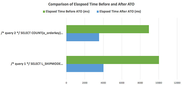


Veerendra Nayak is a Senior Database Solutions Architect with Amazon Web Services.

Building an event-driven application with AWS Lambda and the Amazon Redshift Data API

Post Syndicated from Manash Deb original https://aws.amazon.com/blogs/big-data/building-an-event-driven-application-with-aws-lambda-and-the-amazon-redshift-data-api/

Event–driven applications are becoming popular with many customers, where applications run in response to events. A primary benefit of this architecture is the decoupling of producer and consumer processes, allowing greater flexibility in application design and building decoupled processes.

An example of an even-driven application is an automated workflow being triggered by an event, which runs a series of transformations in the data warehouse. At the end of this workflow, another event gets initiated to notify end-users about the completion of those transformations and that they can start analyzing the transformed dataset.

In this post, we explain how you can easily design a similar event-driven application with Amazon Redshift, AWS Lambda, and Amazon EventBridge. In response to a scheduled event defined in EventBridge, this application automatically triggers a Lambda function to run a stored procedure performing extract, load, and transform (ELT) operations in an Amazon Redshift data warehouse, using its out-of-the-box integration with the Amazon Redshift Data API. This stored procedure copies the source data from Amazon Simple Storage Service (Amazon S3) to Amazon Redshift and aggregates the results. When complete, it sends an event to EventBridge, which triggers a Lambda function to send notification to end-users through Amazon Simple Notification Service (Amazon SNS) to inform them about the availability of updated data in Amazon Redshift.

This event-driven server-less architecture offers greater extensibility and simplicity, making it easier to maintain and faster to release new features, and also reduces the impact of changes. It also simplifies adding other components or third-party products to the application without many changes.

Prerequisites

As a prerequisite for creating the application in this post, you need to set up an Amazon Redshift cluster and associate it with an AWS Identity and Access Management (IAM) role. For more information, see Getting Started with Amazon Redshift.

Solution overview

The following architecture diagram highlights the end-to-end solution, which you can provision automatically with an AWS CloudFormation template.

The workflow includes the following steps:

  1. The EventBridge rule EventBridgeScheduledEventRule is initiated based on a cron schedule.
  2. The rule triggers the Lambda function LambdaRedshiftDataApiETL, with the action run_sql as an input parameter. The Python code for the Lambda function is available in the GitHub repo.
  3. The function performs an asynchronous call to the stored procedure run_elt_process in Amazon Redshift, performing ELT operations using the Amazon Redshift Data API.
  4. The stored procedure uses the Amazon S3 location event-driven-app-with-lambda-redshift/nyc_yellow_taxi_raw/ as the data source for the ELT process. We have pre-populated this with the NYC Yellow Taxi public dataset for the year 2015 to test this solution.
  5. When the stored procedure is complete, the EventBridge rule EventBridgeRedshiftEventRule is triggered automatically to capture the event based on the source parameter redshift-data from the Amazon Redshift Data API.
  6. The rule triggers the Lambda function LambdaRedshiftDataApiETL, with the action notify as an input parameter.
  7. The function uses the SNS topic RedshiftNotificationTopicSNS to send an automated email notification to end-users that the ELT process is complete.

The Amazon Redshift database objects required for this solution are provisioned automatically by the Lambda function LambdaSetupRedshiftObjects as part of the CloudFormation template initiation by invoking the function LambdaRedshiftDataApiETL, which creates the following objects in Amazon Redshift:

  • Table nyc_yellow_taxi, which we use to copy the New York taxi dataset from Amazon S3
  • Materialized view nyc_yellow_taxi_volume_analysis, providing an aggregated view of table
  • Stored procedure run_elt_process to take care of data transformations

The Python code for this function is available in the GitHub repo.

We also use the IAM role LambdaRedshiftDataApiETLRole for the Lambda function and  LambdaRedshiftDataApiETL to allow the following permissions:

  • Federate to the Amazon Redshift cluster through getClusterCredentials permission, avoiding password credentials
  • Initiate queries in the Amazon Redshift cluster through redshift-data API calls
  • Log with Amazon CloudWatch for troubleshooting purposes
  • Send notifications through Amazon SNS

A sample IAM role for this function is available in the GitHub repo.

Lambda is a key service in this solution because it initiates queries in Amazon Redshift using the redshift-data client. Based on the input parameter action, this function can asynchronously initiate Structured Query Language (SQL) statements in Amazon Redshift, thereby avoiding chances of timing out in case of long-running SQL statements[MOU1] [MOU2]   [MOU1]I think we should put reference to Redshift Data API and highlight that there is no need to configure drivers and connections [MOU2]done. It can also publish custom notifications through Amazon SNS. Also, it uses the Amazon Redshift Data API temporary credentials functionality, which allows it to communicate with Amazon Redshift using IAM permissions without the need of any password-based authentication. With the Data API, you also don’t need to configure drivers and connections for your Amazon Redshift cluster, because it’s handled automatically.

Deploying the CloudFormation template

When your Amazon Redshift cluster is set up, use the provided CloudFormation template to automatically create all required resources for this solution in your AWS account. For more information, see Getting started with AWS CloudFormation.

The template requires you to provide the following parameters:

  • RedshiftClusterIdentifier – Cluster identifier for your Amazon Redshift cluster.
  • DbUsername – Amazon Redshift database user name that has access to run the SQL script.
  • DatabaseName – Name of the Amazon Redshift database where the SQL script runs.
  • RedshiftIAMRoleARN – ARN of the IAM role associated with the Amazon Redshift cluster.
  • NotificationEmailId – Email to send event notifications through Amazon SNS.
  • ExecutionSchedule – Cron expression to schedule the ELT process through an EventBridge rule.
  • SqlText – SQL text to run as part of the ELT process. Don’t change the default value call run_elt_process(); if you want to test this solution with the test dataset provided for this post.

The following screenshot shows the stack details on the AWS CloudFormation console.

Testing the pipeline

After setting up the architecture, you should have an automated pipeline to trigger based on the schedule you defined in the EventBridge rule’s cron expression. You can view the CloudWatch logs and troubleshoot issues in the Lambda function. The following screenshot shows the logs for our setup.

You can also view the query status on the Amazon Redshift console, which allows you to view detailed execution plans for the queries you ran. Although the stored procedure may take around 6 minutes to complete, the Lambda function finishes in seconds. This is primarily because the execution from Lambda on Amazon Redshift was asynchronous. Therefore, the function is complete after initiating the process in Amazon Redshift without caring about the query completion.

When this process is complete, you receive the email notification that the ELT process is complete.

You may then view the updated data in your business intelligence tool, like Amazon QuickSight, or query data directly in Amazon Redshift Query Editor (see the following screenshot) to view the most recent data processed by this event-driven architecture.

Conclusion

The Amazon Redshift Data API enables you to painlessly interact with Amazon Redshift and enables you to build event-driven and cloud-native applications. We demonstrated how to build an event-driven application with Amazon Redshift, Lambda, and EventBridge. For more information about the Data API, see Using the Amazon Redshift Data API to interact with Amazon Redshift clusters and Using the Amazon Redshift Data API.


About the Authors

Manash Deb is a Senior Analytics Specialist Solutions Architect. He has worked in different database and data warehousing technologies for more than 15 years.


Debu Panda, a senior product manager at AWS, is an industry leader in analytics, application platform, and database technologies. He has more than 20 years of experience in the IT industry and has published numerous articles on analytics, enterprise Java, and databases and has presented at multiple conferences. He is lead author of the EJB 3 in Action (Manning Publications 2007, 2014) and Middleware Management (Packt).


Fei Peng is a Software Dev Engineer working in the Amazon Redshift team.

Federated API access to Amazon Redshift using an Amazon Redshift connector for Python

Post Syndicated from BP Yau original https://aws.amazon.com/blogs/big-data/federated-api-access-to-amazon-redshift-using-an-amazon-redshift-connector-for-python/

Amazon Redshift is the leading cloud data warehouse that delivers performance 10 times faster at one-tenth of the cost of traditional data warehouses by using massively parallel query execution, columnar storage on high-performance disks, and results caching. You can confidently run mission-critical workloads, even in highly regulated industries, because Amazon Redshift comes with out-of-the-box security and compliance.

You can use your corporate identity providers (IdPs), for example Azure AD, Active Directory Federation Services, Okta, or Ping Federate, with Amazon Redshift to provide single sign-on (SSO) to your users so they can use their IdP accounts to log in and access Amazon Redshift. With federation, you can centralize management and governance of authentication and permissions. For more information about the federation workflow using AWS Identity and Access Management (IAM) and an identity provider, see Federate Database User Authentication Easily with IAM and Amazon Redshift. For this post, we use Okta as our IdP.

If you have personas that use Python on a computer, such as an Amazon Elastic Compute Cloud (Amazon EC2) instance, you generally use an IAM role attached to the EC2 instance for federated access. However, all users who log in to the EC2 instance assume the same IAM role to federate. The Amazon Redshift connector for Python enables IdP authentication for each user who logs in to the computer. This post shows you how to use the Amazon Redshift connector for Python and Okta to enable federated SSO into Amazon Redshift and query your data warehouse using a Python script.

Solution overview

To implement this solution, you complete the following high-level steps:

  1. Configure your Okta IdP, including users, groups, and SAML application.
  2. Configure your AWS service provider, including IdP, IAM policy, and IAM role.
  3. Set up your Amazon Redshift connector.
  4. Check your Amazon Redshift users.
  5. Configure the Python script and Amazon Redshift connector to use your enterprise credentials and sign in to Amazon Redshift to run queries.

The process flow for federated authentication includes the following steps:

  1. The user logs in from a Python script using an Amazon Redshift connector.
  2. The IdP authenticates using the corporate user name and password, and returns a SAML assertion.
  3. The client uses AWS SDK to call AWS Security Token Service (AWS STS) to assume a role with SAML.
  4. AWS STS returns temporary AWS credentials.
  5. The client uses the temporary AWS credentials to connect Amazon Redshift.

The following diagram illustrates this process flow.

Prerequisites

Before starting this walkthrough, you must have the following:

  • An Amazon Redshift cluster. The US East (N. Virginia) Region is preferred because you need to load data from Amazon Simple Storage Service (Amazon S3) in us-east-1.
  • A database user with superuser
  • Python 3.5 or above.
  • Pip.

Configuring your IdP (Okta)

For instructions on setting up your IdP, see steps 1–4 in Federate Amazon Redshift access with Okta as an identity provider.

For step 2, create a user called [email protected] and add it to the sales group. This is the example user that you use in this post. The following screenshot shows your example users.

When the setup is complete, you should see settings similar to the following screenshots. The following screenshot shows your general SAML settings.

The following screenshot shows your attribute statements.

The following screenshot shows the settings for your application embed link, login page, and access error page.

For instructions on setting up advanced IdP configurations, see steps 8–9 in Federate Amazon Redshift access with Okta as an identity provider.

Configuring your service provider (AWS)

To set up the service provider, complete steps 5–7 from Federate Amazon Redshift access with Okta as an identity provider.

For step 7, the Amazon Redshift connector needs the following additional permission:

{
            "Sid": "DescribeClusters",
            "Effect": "Allow",
            "Action": "redshift:DescribeClusters",
            "Resource": "*"
}

The following code shows the example policy used:

{
    "Version": "2012-10-17",
    "Statement": [
        {
            "Sid": "GetClusterCredsStatement",
            "Effect": "Allow",
            "Action": "redshift:GetClusterCredentials",
            "Resource": [
                "arn:aws:redshift:*:*:cluster:<cluster>",
                "arn:aws:redshift:*:*:dbname:<cluster>/<databasename>",
                "arn:aws:redshift:*:*:dbuser:<cluster>/${redshift:DbUser}"
            ]
        },
        {
            "Sid": "DescribeClusters",
            "Effect": "Allow",
            "Action": "redshift:DescribeClusters",
            "Resource": "*"
        },
        {
            "Sid": "CreateClusterUserStatement",
            "Effect": "Allow",
            "Action": "redshift:CreateClusterUser",
            "Resource": [
                "arn:aws:redshift:*:*:dbname:<cluster>/<databasenmae>",
                "arn:aws:redshift:*:*:dbuser:<cluster>/${redshift:DbUser}"
            ]
        },
        {
            "Sid": "RedshiftJoinGroupStatement",
            "Effect": "Allow",
            "Action": "redshift:JoinGroup",
            "Resource": [
                "arn:aws:redshift:*:*:dbgroup:<cluster>/sales"
            ]
        }
    ]
}

When the setup is complete, you should see an IAM role setup similar to the following screenshot.

Setting up your Amazon Redshift connector

The easiest way to get started with redshift_connector is via pip. See the following code:

pip install redshift_connector

After running the command, you see a message indicating redshift_connector was installed successfully:

Successfully installed redshift_connector

Checking Amazon Redshift users

To check your users, connect to your Amazon Redshift cluster using your preferred SQL client as a superuser and enter the following code:

select * from pg_user where usename = '[email protected]';

The query should return zero records, which shows that the corporate user [email protected] doesn’t exist yet in Amazon Redshift. See the following code:

dev=# select * from pg_user where usename = '[email protected]'; 
 usename | usesysid | usecreatedb | usesuper | usecatupd | passwd | valuntil | useconfig 
---------+----------+-------------+----------+-----------+--------+----------+-----------
(0 rows)

Testing the Python script

The next step is to run an example Python script that uses federation to connect to your Amazon Redshift cluster and run some queries. See the following code:

import redshift_connector
import numpy
 
# Connects to Redshift cluster using Okta MFA Browser Plugin
conn = redshift_connector.connect(
    iam=True,
    ssl=True,
    host='<RedshiftClusterEndpoint>',
    port=<RedshiftClusterPortNumber>,
    database='<RedshiftDatabase>',
    db_user='[email protected]',
    cluster_identifier='<RedshiftClusterIdentifier>',
    region='<Region>',
    login_url='<IdPLoginUrl>',
    credentials_provider='BrowserSamlCredentialsProvider',
    user='',
    password=''
)
 
cursor: redshift_connector.Cursor = conn.cursor()
cursor.execute("select current_user")
result: numpy.ndarray = cursor.fetch_numpy_array()
print(result)
 
cursor.execute("create Temp table book(bookname varchar,author‎ varchar)")
cursor.executemany("insert into book (bookname, author‎) values (%s, %s)", [('One Hundred Years of Solitude', 'Gabriel García Márquez'),('A Brief History of Time', 'Stephen Hawking')])
cursor.execute("select * from book")
 
result: numpy.ndarray = cursor.fetch_numpy_array()
print(result)
cursor.execute("drop table book")
conn.commit()
 
conn.close()

Use the following parameters:

  • RedshiftClusterEndpoint – The Amazon Redshift cluster endpoint without a port and database
  • RedshiftClusterPortNumber – The Amazon Redshift port number
  • RedshiftDatabase – The Amazon Redshift database name
  • RedshiftClusterIdentifier – The Amazon Redshift cluster identifier
  • Region – The Region where the cluster is
  • IdPLoginUrl – The IdP (Okta) sign-in URL, which you can get it from the embed link from the Okta SAML application property

After you run the Python script, the Okta sign-in page opens. Sign in with [email protected].

Switch back to your Python environment; it should show three records returned:

$ python3 redshift_connector_okta.py
[['[email protected]']]
[['One Hundred Years of Solitude' 'Gabriel García Márquez']
 ['A Brief History of Time' 'Stephen Hawking']]

[email protected] is returned, showing that the Python script ran under the context of this federated user.

You may now close your browser window.

To check your users, connect to your Amazon Redshift cluster using your preferred SQL client as a superuser and enter the following code:

select * from pg_user where usename = '[email protected]';

The query should return one record, which shows that the database user is automatically created based on the IdP corporate user:

dev=# select * from pg_user where usename = '[email protected]';
      usename      | usesysid | usecreatedb | usesuper | usecatupd |  passwd  | valuntil | useconfig 
-------------------+----------+-------------+----------+-----------+----------+----------+-----------
 [email protected] |      116 | f           | f        | f         | ******** |          | 
(1 row)

Summary

Amazon Redshift supports stringent compliance and security requirements with no extra cost, which makes it ideal for highly regulated industries. With federation, you can centralize management and governance of authentication and permissions by managing users and groups within the enterprise IdP and use them to authenticate to Amazon Redshift. SSO enables users to have a seamless user experience while accessing various applications in the organization.

This post showed you how to set up an Amazon Redshift connector and use Okta as your IdP to enable federated SSO to an Amazon Redshift cluster from a Python script. If you have users such as data scientists that heavily rely on Python scripts, you can follow these steps to set up federated SSO for your organization and manage access privileges to your Amazon Redshift cluster.

If you have any questions or suggestions, please leave a comment or contribute to the project.


About the Authors


BP Yau is a Data Warehouse Specialist Solutions Architect at AWS. His role is to help customers architect big data solutions to process data at scale. Before AWS, he helped Amazon.com Supply Chain Optimization Technologies migrate the Oracle Data Warehouse to Amazon Redshift and built the next generation big data analytics platform using AWS technologies.


Brooke White is a Software Development Engineer at AWS. She enables customers to get the most out of their data through her work on Amazon Redshift drivers. Prior to AWS, she built ETL pipelines and analytics APIs at a San Francisco Bay Area startup.


Ilesh Garish is a Software Development Engineer at AWS. His role is to develop connectors for Amazon Redshift. Prior to AWS, he built database drivers for the Oracle RDBMS, TigerLogic XDMS, and OpenAccess SDK. He worked in the database internal technologies at San Francisco Bay Area startups.

How the ZS COVID-19 Intelligence Engine helps Pharma & Med device manufacturers understand local healthcare needs & gaps at scale

Post Syndicated from Saunak Chandra original https://aws.amazon.com/blogs/big-data/how-the-zs-covid-19-intelligence-engine-helps-pharma-med-device-manufacturers-understand-local-healthcare-needs-gaps-at-scale/

This post is co-written by Parijat Sharma: Principal, Strategy & Transformation, Wenhao Xia: Manager, Data Science, Vineeth Sandadi: Manager, Business Consulting from ZS Associates, Inc, Arianna Tousi: Strategy, Insights and Planning Consultant from ZS, Gopi Vikranth: Associate Principal from ZS. In their own words, “We’re passionately committed to helping our clients and their customers thrive, working side by side to drive customer value and results”.

The COVID-19 trajectory across the US continues to remain unstable and heterogeneous. Although certain cities and counties were able to tame the adverse effects of the pandemic by applying stricter controls on social life, newer hotspots are emerging in different locations sporadically.

Organizations in healthcare, pharma, and biotech are looking to adapt to a rapidly evolving and diverse local market landscape, and restart parts of their operations that are significantly impacted, such as patient support functions, sales, and key account management. Real-time insights into the rapidly evolving COVID-19 situation and its impact on all key stakeholders in the healthcare supply chain, including patients, physicians, and health systems, is a key asset in helping companies adapt based on local market dynamics and remain resilient to future disruptions. However, several life-science companies don’t have these insights because they lack the infrastructure to integrate and manage the relevant datasets at scale and the analytical capabilities to mine the data for the relevant insights.

ZS came into this critical situation and built a data lake on AWS to address these challenges. The primary characteristics of this data lake is that it’s largely open source, which gives ZS a head start to meet the product launch SLA using AWS. This post describes how ZS developed the data lake and brought their proprietary machine learning (ML) models to run on AWS, providing intelligent insight on COVID-19.

What is the ZS COVID-19 Intelligence Engine?

The ZS COVID-19 Intelligence Engine was designed as a customizable capability that does the following:

  • Integrates diverse public and proprietary healthcare datasets in a scalable data warehouse that stores data in a secure and compliant manner
  • Provides advanced descriptive and predictive analytical modules to forecast COVID-19 evolution and its impact on key stakeholders and the treatment journey
  • Packages insights into intuitive preconfigured reports and dashboards for dissemination across an organization

AWS Cloud data and analytics infrastructure

In this section, we dive into the infrastructure components of the ZS COVID-19 Intelligence Engine. The objective was to quickly set up a data lake with an accompanying ingestion mechanism to allow rapid ingestion of public datasets, third-party data, and datasets from AWS Data Exchange.

The overall data processing solution is based on ZS’s REVO™ data management product, which uses Apache Spark on Amazon EMR. The Spark engine processes and transforms raw data into structured data that is ready for interactive analysis. The raw data comes in compressed text delimited format ranging from 100 MBs to 15 GB. After the data is cleansed and rules applied, the processed data is staged in Amazon Simple Storage Service (Amazon S3) buckets in Apache Parquet format. This data is selectively loaded into an Amazon Redshift cluster for fast interactive querying and repetitive analysis on subsets of data.

The Intelligence Engine also uses a powerful Amazon Elastic Compute Cloud (Amazon EC2) instance to run ML workloads, which predicts future COVID-19 caseloads at the county level. The prediction models run daily on a compute-optimized EC2 C5.24xlarge On-Demand Instance, allowing rapid turnaround of prediction results and saving overall cost for using On-Demand Instances.

ZS uses Amazon Redshift as the data warehouse in this architecture. Amazon Redshift is easy to launch and maintain and can quickly run analytical queries on large normalized datasets using standard ANSI SQL. After the raw data gets processed using ZS’s REVO™, the curated data is loaded into Amazon Redshift to run interactive analytical queries. The queries generate insights specific to local geography, county, and healthcare systems, and run on Amazon Redshift tables consisting of anonymized patient data. The Amazon Redshift cluster uses On-Demand Instances and is sized to accommodate 25 TB of data at the time of this product launch. Typical interactive queries include joining data across large tables, up to 1.5 billion rows in the main table.

The following diagram illustrates this architecture:

The ZS COVID-19 data lake has several benefits and applicable use cases:

  • Streamlined data procurement processes – Eliminates the need for multiple ZS teams to procure, ingest, and process the same datasets separately
  • Optimized common usage across clients and business questions – ZS uses this capability to publish common derivations of data that can then be utilized across different ZS teams and use cases to create a single version of truth
  • Cross-functional processes and requirements – Some analytics use cases require cross-functional data and are significantly hampered by the ability of a user to access various data sources in one place—a data lake enables this by design
  • Connected healthcare data – Due to developing common standards and integrating with MDM and ontologies, data from the public domain can be compliantly integrated with pharma manufacturer-specific data sources to enable seamless analytics on the data lake

Comprehensive healthcare data lake

At its core, the Intelligence Engine builds a scalable and integrated repository of diverse public and proprietary data sources. These datasets range in variety, volume, and velocity:

  • COVID-19 incidence – There are several COVID-specific datasets that the public has become accustomed to viewing over the past several months, such as Johns Hopkins incidence tracking and IHME predictive data, which describes how the disease has been progressing over time and even into the future. This data tends to be at either the state or county level and is often refreshed daily. The data lake solution contains the entire history for these datasets, which, taken together, spans into the hundreds of gigabytes in size. In addition to these sources, ZS’ proprietary predictive models add an additional element of accuracy and are customized with ZS-specific insights.
  • Government policies – Government policy data, which is mostly being used from AWS Data Exchange on behalf of the New York Times, explains the current state of government mandates and recommendations for varying degrees of lockdown or reopening as it pertains to the pandemic. This data is much smaller in volume, well under 1 GB total.
  • Insurance claims at patient level – Thanks to the partnership with Symphony Health, ZS have had the opportunity to analyze and expose patient claims data that can be attributed to the specific hospital account or healthcare provider for which that claim took place. The insurance claims data is the largest volume of data—close to 15 TB—contributing to the ZS COVID-19 Intelligence Engine. ZS’ data engineering team has wrangled these large datasets with the help of Amazon EMR for aggregating and processing metrics, which are then stored in Amazon Redshift in a transformed version that is much smaller and can be more easily understood than the original raw datasets.
  • HCP to site of care affiliations – Thanks to the partnership with Definitive Healthcare, ZS are in the process of integrating best-in-class physician-hospital and clinic affiliations from Definitive Healthcare with patient claims from Symphony to help assess available healthcare capacity and evolving approaches to care delivery and type of care being delivered by disease area.
  • Other Intelligence engine data sources –
    • State testing rates
    • Mobility
    • Demographics and social determinants of health
    • Provider access and affinity for pharma commercial engagement (from ZS affinity/access monitor)
    • Automated data ingestors for a variety of pharma manufacturer-specific data sources including specialty pharmacy and hub transactions, sales force activity, customer digital engagement, and more

Predictive models for COVID-19 projections and healthcare demand-supply gaps at a local level

To drive decision-making at a local level, ZS required more granular projections of COVID-19 disease spread than what’s publicly available at a state or national level. Therefore, as part of the Intelligence Engine, the ZS data science team aimed to developed an ensemble model of COVID-19 projections at the county level to identify emerging local healthcare gaps along different phases of the treatment process.

Developing a locally predictive model has many challenges, and ZS believe that no single model can capture all the virtually infinite drivers and factors contributing to disease spread within a specific geographic area. Therefore, the ZS data science team behind the COVID-19 projections has implemented multiple projection models, each with their own set of input data sources, assumptions, and parameters. This allows to increase the accuracy of the projection while retaining a level of stability and interpretability of tge model. These models include:

  • Statistical curve fitting model – A disease progression curve using a Generalized Gaussian Cumulative Distribution Function, optimized to minimize prediction error of COVID-19 cases and deaths
  • SEIR model – Traditional epidemiological disease progression model (pathway of Susceptible – Exposed – Infectious – Recovered) combined with traditional ML on model parameters
  • Agent-based simulation – County-level simulation of individual interactions between people within the county

Obtaining a more granular view of future virus spread at a local level is critical in order to provide support for challenges in specific sites of care. Accurately projecting cases at the county level can be difficult for many reasons. Counties with low current case counts means that the model has little historical data to learn from (both in time since first infection and in magnitude of cases). Additionally, forecasts can be sensitive to many variables, and the current second wave of COVID-19 infections adds additional complications to tracking the spread of the virus.

To combat some of these difficulties, ZS implemented a two-phased approach to generate county-level projections. Counties with a long enough history of virus spread are projected independently using the three disease progression models we outlined, whereas counties with limited history are projected using a combination of state-level projections and social determinants of health factors that are predictive of disease spread (for example, age distribution in a certain county).

As the world around us continues to evolve and the COVID-19 situation with it, the ZS data science team is also working to adapt the model alongside the current situation. Currently, model adaptability and its self-learning ability are continuing to improve to better adapt to the onset of the second wave of the virus. Additional parameters and re-optimizations are happening daily as the situation develops.

Following image shows the Input data sources, modeling techniques and outputs from ZS COVID-19 projection models:

Analyzing and predicting local non-COVID-19 treatment gaps and their drivers

Several flexible analytical tools can be used to evaluate barriers along the disease treatment journey for non-COVID-19 diseases at the local geography level, their evolution over time with COVID-19, and their underlying drivers. These tools summarize local changes in and the underlying drivers of the following:

  • New patient diagnosis
  • Changes in treatment approaches and drugs used
  • Patient affordability and access to medications
  • Persistency and compliance to treatment
  • Healthcare demand, patients needing care and supply, provider capacity to offer care

Following image represents output from the Intelligence Engine illustrating local variations in Healthcare gaps:

Intuitive visualization capabilities

The solution has two intuitive visualization capabilities:

  • COVID-19 monitor – A public access dashboard with insights on historical and future predictions of trajectories of COVID-19 incidences and hospital capacity. These insights are available at the state level and further and allow you to drill into individual counties. The individual county-level view allows you to not only understand the severity of COVID-19 in that area, but also better understand how that county compares to other counties within the same state and observe what policies their local governments have set for the shutdown and reopening process.
  • Treatment finder: A second public access dashboard with near-real-time insights into individual hospital and physician group availability to treat patients for prominent non-COVID-19 diseases. This dashboard allows you to select a specific non-COVID-19 disease and identify the estimated number of COIVD-19-infected people in their geography with the disease, mortality rates, and the individual providers that are accepting patients with a specific disease and health insurance.

Following image represents Intelligence Engine screen with COVID-19 insights for a selected county:

Following image represents Intelligence engine screen that allows patients to find Hospitals / Physician offices that are open & accepting patients:

Conclusion

At its core, the ZS Intelligence Engine is a real-time planning tool. The rich set of AWS services and technologies make it possible to ingest data from various third-party sources—public and proprietary sources alike. AWS services used to build the architecture can run on open technologies. For example, building the the data lake would not have been possible  without Amazon EMR and Amazon EC2. ZS had already been using Apache spark-based EMR instances—the service behind the REVOTM tool—prior to COVID-19 hitting us. ZS can run its ML models cost-effectively by using EC2 On-Demand Instances. Finally, using Amazon Redshift as a data warehouse solution allows ZS to provide COVID-19 analytical insights efficiently and cost-effectively.

Since the project went live, ZS has catered this product to at least six customers in pharma, biotech, and medical device spaces. They are using this product in a variety of ways, including but not limited to:

  • Refining the forecast relating the COVID-19 trajectory to estimate demand for their products
  • Assessing the level of openness of healthcare facilities to understand where patients across therapy areas are being treated
  • Determining which patients and communities to support, because COVID-19 impacts attitudes and concerns regarding immunity and drug use, and greater unemployment means more reimbursement support requirements
  • Readying the education and engagement field force for a mix of in-person and virtual interactions
  • Preparing the supply chain to ensure continuity of care

To try out the analysis yourself, see ZS’s COVID-19 Intelligence Engine.


About the  Authors

Saunak is a Sr. Solutions Architect with AWS helping customers and partners build data warehouse and scalable data platform on AWS.


Parijat is the current lead of strategy and transformation at ZS. He focuses on mid to small clients that are ready for a transformational process to commercialize new products/portfolio, purchase/sell assets or expand into new markets.


Wenhao has over 10 years of experience in various data science and advanced analytics field. During his time at ZS, he has helped both to build and popularize data science capabilities across many organizations.


Vineeth works with Pharmaceutical & Biotech manufacturers on a  broad-spectrum of Commercial issues including Commercial Analytics, Organized provider Strategy & Resource Planning & Deployment.


Arianna is a Strategy, Insights and Planning Consultant in ZS’ High Tech practice. Arianna has extensive experience in working with clients across industries with go to market strategy and commercial effectiveness issues.


Gopi Vikranth is an Associate Principal in ZS’ High Tech Practice. He has extensive experience in helping clients across Retail, HiTech, Hospitality, Pharmaceutical & Insurance sectors leverage BigData & Analytics to drive Topline growth.


AWS serverless data analytics pipeline reference architecture

Post Syndicated from Praful Kava original https://aws.amazon.com/blogs/big-data/aws-serverless-data-analytics-pipeline-reference-architecture/

Onboarding new data or building new analytics pipelines in traditional analytics architectures typically requires extensive coordination across business, data engineering, and data science and analytics teams to first negotiate requirements, schema, infrastructure capacity needs, and workload management.

For a large number of use cases today however, business users, data scientists, and analysts are demanding easy, frictionless, self-service options to build end-to-end data pipelines because it’s hard and inefficient to predefine constantly changing schemas and spend time negotiating capacity slots on shared infrastructure. The exploratory nature of machine learning (ML) and many analytics tasks means you need to rapidly ingest new datasets and clean, normalize, and feature engineer them without worrying about operational overhead when you have to think about the infrastructure that runs data pipelines.

A serverless data lake architecture enables agile and self-service data onboarding and analytics for all data consumer roles across a company. By using AWS serverless technologies as building blocks, you can rapidly and interactively build data lakes and data processing pipelines to ingest, store, transform, and analyze petabytes of structured and unstructured data from batch and streaming sources, all without needing to manage any storage or compute infrastructure.

In this post, we first discuss a layered, component-oriented logical architecture of modern analytics platforms and then present a reference architecture for building a serverless data platform that includes a data lake, data processing pipelines, and a consumption layer that enables several ways to analyze the data in the data lake without moving it (including business intelligence (BI) dashboarding, exploratory interactive SQL, big data processing, predictive analytics, and ML).

Logical architecture of modern data lake centric analytics platforms

The following diagram illustrates the architecture of a data lake centric analytics platform.

You can envision a data lake centric analytics architecture as a stack of six logical layers, where each layer is composed of multiple components. A layered, component-oriented architecture promotes separation of concerns, decoupling of tasks, and flexibility. These in turn provide the agility needed to quickly integrate new data sources, support new analytics methods, and add tools required to keep up with the accelerating pace of changes in the analytics landscape. In the following sections, we look at the key responsibilities, capabilities, and integrations of each logical layer.

Ingestion layer

The ingestion layer is responsible for bringing data into the data lake. It provides the ability to connect to internal and external data sources over a variety of protocols. It can ingest batch and streaming data into the storage layer. The ingestion layer is also responsible for delivering ingested data to a diverse set of targets in the data storage layer (including the object store, databases, and warehouses).

Storage layer

The storage layer is responsible for providing durable, scalable, secure, and cost-effective components to store vast quantities of data. It supports storing unstructured data and datasets of a variety of structures and formats. It supports storing source data as-is without first needing to structure it to conform to a target schema or format. Components from all other layers provide easy and native integration with the storage layer. To store data based on its consumption readiness for different personas across organization, the storage layer is organized into the following zones:

  • Landing zone – The storage area where components from the ingestion layer land data. This is a transient area where data is ingested from sources as-is. Typically, data engineering personas interact with the data stored in this zone.
  • Raw zone – After the preliminary quality checks, the data from the landing zone is moved to the raw zone for permanent storage. Here, data is stored in its original format. Having all data from all sources permanently stored in the raw zone provides the ability to “replay” downstream data processing in case of errors or data loss in downstream storage zones. Typically, data engineering and data science personas interact with the data stored in this zone.
  • Curated zone – This zone hosts data that is in the most consumption-ready state and conforms to organizational standards and data models. Datasets in the curated zone are typically partitioned, cataloged, and stored in formats that support performant and cost-effective access by the consumption layer. The processing layer creates datasets in the curated zone after cleaning, normalizing, standardizing, and enriching data from the raw zone. All personas across organizations use the data stored in this zone to drive business decisions.

Cataloging and search layer

The cataloging and search layer is responsible for storing business and technical metadata about datasets hosted in the storage layer. It provides the ability to track schema and the granular partitioning of dataset information in the lake. It also supports mechanisms to track versions to keep track of changes to the metadata. As the number of datasets in the data lake grows, this layer makes datasets in the data lake discoverable by providing search capabilities.

Processing layer

The processing layer is responsible for transforming data into a consumable state through data validation, cleanup, normalization, transformation, and enrichment. It’s responsible for advancing the consumption readiness of datasets along the landing, raw, and curated zones and registering metadata for the raw and transformed data into the cataloging layer. The processing layer is composed of purpose-built data-processing components to match the right dataset characteristic and processing task at hand. The processing layer can handle large data volumes and support schema-on-read, partitioned data, and diverse data formats. The processing layer also provides the ability to build and orchestrate multi-step data processing pipelines that use purpose-built components for each step.

Consumption layer

The consumption layer is responsible for providing scalable and performant tools to gain insights from the vast amount of data in the data lake. It democratizes analytics across all personas across the organization through several purpose-built analytics tools that support analysis methods, including SQL, batch analytics, BI dashboards, reporting, and ML. The consumption layer natively integrates with the data lake’s storage, cataloging, and security layers. Components in the consumption layer support schema-on-read, a variety of data structures and formats, and use data partitioning for cost and performance optimization.

Security and governance layer

The security and governance layer is responsible for protecting the data in the storage layer and processing resources in all other layers. It provides mechanisms for access control, encryption, network protection, usage monitoring, and auditing. The security layer also monitors activities of all components in other layers and generates a detailed audit trail. Components of all other layers provide native integration with the security and governance layer.

Serverless data lake centric analytics architecture

To compose the layers described in our logical architecture, we introduce a reference architecture that uses AWS serverless and managed services. In this approach, AWS services take over the heavy lifting of the following:

  • Providing and managing scalable, resilient, secure, and cost-effective infrastructural components
  • Ensuring infrastructural components natively integrate with each other

This reference architecture allows you to focus more time on rapidly building data and analytics pipelines. It significantly accelerates new data onboarding and driving insights from your data. The AWS serverless and managed components enable self-service across all data consumer roles by providing the following key benefits:

  • Easy configuration-driven use
  • Freedom from infrastructure management
  • Pay-per-use pricing model

The following diagram illustrates this architecture.

Ingestion layer

The ingestion layer in our serverless architecture is composed of a set of purpose-built AWS services to enable data ingestion from a variety of sources. Each of these services enables simple self-service data ingestion into the data lake landing zone and provides integration with other AWS services in the storage and security layers. Individual purpose-built AWS services match the unique connectivity, data format, data structure, and data velocity requirements of operational database sources, streaming data sources, and file sources.

Operational database sources

Typically, organizations store their operational data in various relational and NoSQL databases. AWS Data Migration Service (AWS DMS) can connect to a variety of operational RDBMS and NoSQL databases and ingest their data into Amazon Simple Storage Service (Amazon S3) buckets in the data lake landing zone. With AWS DMS, you can first perform a one-time import of the source data into the data lake and replicate ongoing changes happening in the source database. AWS DMS encrypts S3 objects using AWS Key Management Service (AWS KMS) keys as it stores them in the data lake. AWS DMS is a fully managed, resilient service and provides a wide choice of instance sizes to host database replication tasks.

AWS Lake Formation provides a scalable, serverless alternative, called blueprints, to ingest data from AWS native or on-premises database sources into the landing zone in the data lake. A Lake Formation blueprint is a predefined template that generates a data ingestion AWS Glue workflow based on input parameters such as source database, target Amazon S3 location, target dataset format, target dataset partitioning columns, and schedule. A blueprint-generated AWS Glue workflow implements an optimized and parallelized data ingestion pipeline consisting of crawlers, multiple parallel jobs, and triggers connecting them based on conditions. For more information, see Integrating AWS Lake Formation with Amazon RDS for SQL Server.

Streaming data sources

The ingestion layer uses Amazon Kinesis Data Firehose to receive streaming data from internal and external sources. With a few clicks, you can configure a Kinesis Data Firehose API endpoint where sources can send streaming data such as clickstreams, application and infrastructure logs and monitoring metrics, and IoT data such as devices telemetry and sensor readings. Kinesis Data Firehose does the following:

  • Buffers incoming streams
  • Batches, compresses, transforms, and encrypts the streams
  • Stores the streams as S3 objects in the landing zone in the data lake

Kinesis Data Firehose natively integrates with the security and storage layers and can deliver data to Amazon S3, Amazon Redshift, and Amazon Elasticsearch Service (Amazon ES) for real-time analytics use cases. Kinesis Data Firehose is serverless, requires no administration, and has a cost model where you pay only for the volume of data you transmit and process through the service. Kinesis Data Firehose automatically scales to adjust to the volume and throughput of incoming data.

File sources

Many applications store structured and unstructured data in files that are hosted on Network Attached Storage (NAS) arrays. Organizations also receive data files from partners and third-party vendors. Analyzing data from these file sources can provide valuable business insights.

Internal file shares

AWS DataSync can ingest hundreds of terabytes and millions of files from NFS and SMB enabled NAS devices into the data lake landing zone. DataSync automatically handles scripting of copy jobs, scheduling and monitoring transfers, validating data integrity, and optimizing network utilization. DataSync can perform one-time file transfers and monitor and sync changed files into the data lake. DataSync is fully managed and can be set up in minutes.

Partner data files

FTP is most common method for exchanging data files with partners. The AWS Transfer Family is a serverless, highly available, and scalable service that supports secure FTP endpoints and natively integrates with Amazon S3. Partners and vendors transmit files using SFTP protocol, and the AWS Transfer Family stores them as S3 objects in the landing zone in the data lake. The AWS Transfer Family supports encryption using AWS KMS and common authentication methods including AWS Identity and Access Management (IAM) and Active Directory.

Data APIs

Organizations today use SaaS and partner applications such as Salesforce, Marketo, and Google Analytics to support their business operations. Analyzing SaaS and partner data in combination with internal operational application data is critical to gaining 360-degree business insights. Partner and SaaS applications often provide API endpoints to share data.

SaaS APIs

The ingestion layer uses AWS AppFlow to easily ingest SaaS applications data into the data lake. With a few clicks, you can set up serverless data ingestion flows in AppFlow. Your flows can connect to SaaS applications (such as SalesForce, Marketo, and Google Analytics), ingest data, and store it in the data lake. You can schedule AppFlow data ingestion flows or trigger them by events in the SaaS application. Ingested data can be validated, filtered, mapped and masked before storing in the data lake. AppFlow natively integrates with authentication, authorization, and encryption services in the security and governance layer.

Partner APIs

To ingest data from partner and third-party APIs, organizations build or purchase custom applications that connect to APIs, fetch data, and create S3 objects in the landing zone by using AWS SDKs. These applications and their dependencies can be packaged into Docker containers and hosted on AWS Fargate. Fargate is a serverless compute engine for hosting Docker containers without having to provision, manage, and scale servers. Fargate natively integrates with AWS security and monitoring services to provide encryption, authorization, network isolation, logging, and monitoring to the application containers.

AWS Glue Python shell jobs also provide serverless alternative to build and schedule data ingestion jobs that can interact with partner APIs by using native, open-source, or partner-provided Python libraries. AWS Glue provides out-of-the-box capabilities to schedule singular Python shell jobs or include them as part of a more complex data ingestion workflow built on AWS Glue workflows.

Third-party data sources

Your organization can gain a business edge by combining your internal data with third-party datasets such as historical demographics, weather data, and consumer behavior data. AWS Data Exchange provides a serverless way to find, subscribe to, and ingest third-party data directly into S3 buckets in the data lake landing zone. You can ingest a full third-party dataset and then automate detecting and ingesting revisions to that dataset. AWS Data Exchange is serverless and lets you find and ingest third-party datasets with a few clicks.

Storage layer

Amazon S3 provides the foundation for the storage layer in our architecture. Amazon S3 provides virtually unlimited scalability at low cost for our serverless data lake. Data is stored as S3 objects organized into landing, raw, and curated zone buckets and prefixes. Amazon S3 encrypts data using keys managed in AWS KMS. IAM policies control granular zone-level and dataset-level access to various users and roles. Amazon S3 provides 99.99 % of availability and 99.999999999 % of durability, and charges only for the data it stores. To significantly reduce costs, Amazon S3 provides colder tier storage options called Amazon S3 Glacier and S3 Glacier Deep Archive. To automate cost optimizations, Amazon S3 provides configurable lifecycle policies and intelligent tiering options to automate moving older data to colder tiers. AWS services in our ingestion, cataloging, processing, and consumption layers can natively read and write S3 objects. Additionally, hundreds of third-party vendor and open-source products and services provide the ability to read and write S3 objects.

Data of any structure (including unstructured data) and any format can be stored as S3 objects without needing to predefine any schema. This enables services in the ingestion layer to quickly land a variety of source data into the data lake in its original source format. After the data is ingested into the data lake, components in the processing layer can define schema on top of S3 datasets and register them in the cataloging layer. Services in the processing and consumption layers can then use schema-on-read to apply the required structure to data read from S3 objects. Datasets stored in Amazon S3 are often partitioned to enable efficient filtering by services in the processing and consumption layers.

Cataloging and search layer

A data lake typically hosts a large number of datasets, and many of these datasets have evolving schema and new data partitions. A central Data Catalog that manages metadata for all the datasets in the data lake is crucial to enabling self-service discovery of data in the data lake. Additionally, separating metadata from data into a central schema enables schema-on-read for the processing and consumption layer components.

In our architecture, Lake Formation provides the central catalog to store and manage metadata for all datasets hosted in the data lake. Organizations manage both technical metadata (such as versioned table schemas, partitioning information, physical data location, and update timestamps) and business attributes (such as data owner, data steward, column business definition, and column information sensitivity) of all their datasets in Lake Formation. Services such as AWS Glue, Amazon EMR, and Amazon Athena natively integrate with Lake Formation and automate discovering and registering dataset metadata into the Lake Formation catalog. Additionally, Lake Formation provides APIs to enable metadata registration and management using custom scripts and third-party products. AWS Glue crawlers in the processing layer can track evolving schemas and newly added partitions of datasets in the data lake, and add new versions of corresponding metadata in the Lake Formation catalog.

Lake Formation provides the data lake administrator a central place to set up granular table- and column-level permissions for databases and tables hosted in the data lake. After Lake Formation permissions are set up, users and groups can access only authorized tables and columns using multiple processing and consumption layer services such as Athena, Amazon EMR, AWS Glue, and Amazon Redshift Spectrum.

Processing layer

The processing layer in our architecture is composed of two types of components:

  • Components used to create multi-step data processing pipelines
  • Components to orchestrate data processing pipelines on schedule or in response to event triggers (such as ingestion of new data into the landing zone)

AWS Glue and AWS Step Functions provide serverless components to build, orchestrate, and run pipelines that can easily scale to process large data volumes. Multi-step workflows built using AWS Glue and Step Functions can catalog, validate, clean, transform, and enrich individual datasets and advance them from landing to raw and raw to curated zones in the storage layer.

AWS Glue is a serverless, pay-per-use ETL service for building and running Python or Spark jobs (written in Scala or Python) without requiring you to deploy or manage clusters. AWS Glue automatically generates the code to accelerate your data transformations and loading processes. AWS Glue ETL builds on top of Apache Spark and provides commonly used out-of-the-box data source connectors, data structures, and ETL transformations to validate, clean, transform, and flatten data stored in many open-source formats such as CSV, JSON, Parquet, and Avro. AWS Glue ETL also provides capabilities to incrementally process partitioned data.

Additionally, you can use AWS Glue to define and run crawlers that can crawl folders in the data lake, discover datasets and their partitions, infer schema, and define tables in the Lake Formation catalog. AWS Glue provides more than a dozen built-in classifiers that can parse a variety of data structures stored in open-source formats. AWS Glue also provides triggers and workflow capabilities that you can use to build multi-step end-to-end data processing pipelines that include job dependencies and running parallel steps. You can schedule AWS Glue jobs and workflows or run them on demand. AWS Glue natively integrates with AWS services in storage, catalog, and security layers.

Step Functions is a serverless engine that you can use to build and orchestrate scheduled or event-driven data processing workflows. You use Step Functions to build complex data processing pipelines that involve orchestrating steps implemented by using multiple AWS services such as AWS Glue, AWS Lambda, Amazon Elastic Container Service (Amazon ECS) containers, and more. Step Functions provides visual representations of complex workflows and their running state to make them easy to understand. It manages state, checkpoints, and restarts of the workflow for you to make sure that the steps in your data pipeline run in order and as expected. Built-in try/catch, retry, and rollback capabilities deal with errors and exceptions automatically.

Consumption layer

The consumption layer in our architecture is composed using fully managed, purpose-built, analytics services that enable interactive SQL, BI dashboarding, batch processing, and ML.

Interactive SQL

Athena is an interactive query service that enables you to run complex ANSI SQL against terabytes of data stored in Amazon S3 without needing to first load it into a database. Athena queries can analyze structured, semi-structured, and columnar data stored in open-source formats such as CSV, JSON, XML Avro, Parquet, and ORC. Athena uses table definitions from Lake Formation to apply schema-on-read to data read from Amazon S3.

Athena is serverless, so there is no infrastructure to set up or manage, and you pay only for the amount of data scanned by the queries you run. Athena provides faster results and lower costs by reducing the amount of data it scans by using dataset partitioning information stored in the Lake Formation catalog. You can run queries directly on the Athena console of submit them using Athena JDBC or ODBC endpoints.

Athena natively integrates with AWS services in the security and monitoring layer to support authentication, authorization, encryption, logging, and monitoring. It supports table- and column-level access controls defined in the Lake Formation catalog.

Data warehousing and batch analytics

Amazon Redshift is a fully managed data warehouse service that can host and process petabytes of data and run thousands highly performant queries in parallel. Amazon Redshift uses a cluster of compute nodes to run very low-latency queries to power interactive dashboards and high-throughput batch analytics to drive business decisions. You can run Amazon Redshift queries directly on the Amazon Redshift console or submit them using the JDBC/ODBC endpoints provided by Amazon Redshift.

Amazon Redshift provides the capability, called Amazon Redshift Spectrum, to perform in-place queries on structured and semi-structured datasets in Amazon S3 without needing to load it into the cluster. Amazon Redshift Spectrum can spin up thousands of query-specific temporary nodes to scan exabytes of data to deliver fast results. Organizations typically load most frequently accessed dimension and fact data into an Amazon Redshift cluster and keep up to exabytes of structured, semi-structured, and unstructured historical data in Amazon S3. Amazon Redshift Spectrum enables running complex queries that combine data in a cluster with data on Amazon S3 in the same query.

Amazon Redshift provides native integration with Amazon S3 in the storage layer, Lake Formation catalog, and AWS services in the security and monitoring layer.

Business intelligence

Amazon QuickSight provides a serverless BI capability to easily create and publish rich, interactive dashboards. QuickSight enriches dashboards and visuals with out-of-the-box, automatically generated ML insights such as forecasting, anomaly detection, and narrative highlights. QuickSight natively integrates with Amazon SageMaker to enable additional custom ML model-based insights to your BI dashboards. You can access QuickSight dashboards from any device using a QuickSight app, or you can embed the dashboard into web applications, portals, and websites.

QuickSight allows you to directly connect to and import data from a wide variety of cloud and on-premises data sources. These include SaaS applications such as Salesforce, Square, ServiceNow, Twitter, GitHub, and JIRA; third-party databases such as Teradata, MySQL, Postgres, and SQL Server; native AWS services such as Amazon Redshift, Athena, Amazon S3, Amazon Relational Database Service (Amazon RDS), and Amazon Aurora; and private VPC subnets. You can also upload a variety of file types including XLS, CSV, JSON, and Presto.

To achieve blazing fast performance for dashboards, QuickSight provides an in-memory caching and calculation engine called SPICE. SPICE automatically replicates data for high availability and enables thousands of users to simultaneously perform fast, interactive analysis while shielding your underlying data infrastructure. QuickSight automatically scales to tens of thousands of users and provides a cost-effective, pay-per-session pricing model.

QuickSight allows you to securely manage your users and content via a comprehensive set of security features, including role-based access control, active directory integration, AWS CloudTrail auditing, single sign-on (IAM or third-party), private VPC subnets, and data backup.

Predictive analytics and ML

Amazon SageMaker is a fully managed service that provides components to build, train, and deploy ML models using an interactive development environment (IDE) called Amazon SageMaker Studio. In Amazon SageMaker Studio, you can upload data, create new notebooks, train and tune models, move back and forth between steps to adjust experiments, compare results, and deploy models to production, all in one place by using a unified visual interface. Amazon SageMaker also provides managed Jupyter notebooks that you can spin up with just a few clicks. Amazon SageMaker notebooks provide elastic compute resources, git integration, easy sharing, pre-configured ML algorithms, dozens of out-of-the-box ML examples, and AWS Marketplace integration, which enables easy deployment of hundreds of pre-trained algorithms. Amazon SageMaker notebooks are preconfigured with all major deep learning frameworks, including TensorFlow, PyTorch, Apache MXNet, Chainer, Keras, Gluon, Horovod, Scikit-learn, and Deep Graph Library.

ML models are trained on Amazon SageMaker managed compute instances, including highly cost-effective Amazon Elastic Compute Cloud (Amazon EC2) Spot Instances. You can organize multiple training jobs by using Amazon SageMaker Experiments. You can build training jobs using Amazon SageMaker built-in algorithms, your custom algorithms, or hundreds of algorithms you can deploy from AWS Marketplace. Amazon SageMaker Debugger provides full visibility into model training jobs. Amazon SageMaker also provides automatic hyperparameter tuning for ML training jobs.

You can deploy Amazon SageMaker trained models into production with a few clicks and easily scale them across a fleet of fully managed EC2 instances. You can choose from multiple EC2 instance types and attach cost-effective GPU-powered inference acceleration. After the models are deployed, Amazon SageMaker can monitor key model metrics for inference accuracy and detect any concept drift.

Amazon SageMaker provides native integrations with AWS services in the storage and security layers.

Security and governance layer

Components across all layers of our architecture protect data, identities, and processing resources by natively using the following capabilities provided by the security and governance layer.

Authentication and authorization

IAM provides user-, group-, and role-level identity to users and the ability to configure fine-grained access control for resources managed by AWS services in all layers of our architecture. IAM supports multi-factor authentication and single sign-on through integrations with corporate directories and open identity providers such as Google, Facebook, and Amazon.

Lake Formation provides a simple and centralized authorization model for tables hosted in the data lake. After implemented in Lake Formation, authorization policies for databases and tables are enforced by other AWS services such as Athena, Amazon EMR, QuickSight, and Amazon Redshift Spectrum. In Lake Formation, you can grant or revoke database-, table-, or column-level access for IAM users, groups, or roles defined in the same account hosting the Lake Formation catalog or another AWS account. The simple grant/revoke-based authorization model of Lake Formation considerably simplifies the previous IAM-based authorization model that relied on separately securing S3 data objects and metadata objects in the AWS Glue Data Catalog.

Encryption

AWS KMS provides the capability to create and manage symmetric and asymmetric customer-managed encryption keys. AWS services in all layers of our architecture natively integrate with AWS KMS to encrypt data in the data lake. It supports both creating new keys and importing existing customer keys. Access to the encryption keys is controlled using IAM and is monitored through detailed audit trails in CloudTrail.

Network protection

Our architecture uses Amazon Virtual Private Cloud (Amazon VPC) to provision a logically isolated section of the AWS Cloud (called VPC) that is isolated from the internet and other AWS customers. AWS VPC provides the ability to choose your own IP address range, create subnets, and configure route tables and network gateways. AWS services from other layers in our architecture launch resources in this private VPC to protect all traffic to and from these resources.

Monitoring and logging

AWS services in all layers of our architecture store detailed logs and monitoring metrics in AWS CloudWatch. CloudWatch provides the ability to analyze logs, visualize monitored metrics, define monitoring thresholds, and send alerts when thresholds are crossed.

All AWS services in our architecture also store extensive audit trails of user and service actions in CloudTrail. CloudTrail provides event history of your AWS account activity, including actions taken through the AWS Management Console, AWS SDKs, command line tools, and other AWS services. This event history simplifies security analysis, resource change tracking, and troubleshooting. In addition, you can use CloudTrail to detect unusual activity in your AWS accounts. These capabilities help simplify operational analysis and troubleshooting.

Additional considerations

In this post, we talked about ingesting data from diverse sources and storing it as S3 objects in the data lake and then using AWS Glue to process ingested datasets until they’re in a consumable state. This architecture enables use cases needing source-to-consumption latency of a few minutes to hours. In a future post, we will evolve our serverless analytics architecture to add a speed layer to enable use cases that require source-to-consumption latency in seconds, all while aligning with the layered logical architecture we introduced.

Conclusion

With AWS serverless and managed services, you can build a modern, low-cost data lake centric analytics architecture in days. A decoupled, component-driven architecture allows you to start small and quickly add new purpose-built components to one of six architecture layers to address new requirements and data sources.

We invite you to read the following posts that contain detailed walkthroughs and sample code for building the components of the serverless data lake centric analytics architecture:


About the Authors

Praful Kava is a Sr. Specialist Solutions Architect at AWS. He guides customers to design and engineer Cloud scale Analytics pipelines on AWS. Outside work, he enjoys travelling with his family and exploring new hiking trails.


Changbin Gong is a Senior Solutions Architect at Amazon Web Services (AWS). He engages with customers to create innovative solutions that address customer business problems and accelerate the adoption of AWS services. In his spare time, Changbin enjoys reading, running, and traveling.