Tag Archives: Data Catalog

Announcing the Cloudflare Data Platform: ingest, store, and query your data directly on Cloudflare

Post Syndicated from Micah Wylde original https://blog.cloudflare.com/cloudflare-data-platform/

For Developer Week in April 2025, we announced the public beta of R2 Data Catalog, a fully managed Apache Iceberg catalog on top of Cloudflare R2 object storage. Today, we are building on that foundation with three launches:

  • Cloudflare Pipelines receives events sent via Workers or HTTP, transforms them with SQL, and ingests them into Iceberg or as files on R2

  • R2 Data Catalog manages the Iceberg metadata and now performs ongoing maintenance, including compaction, to improve query performance

  • R2 SQL is our in-house distributed SQL engine, designed to perform petabyte-scale queries over your data in R2

Together, these products make up the Cloudflare Data Platform, a complete solution for ingesting, storing, and querying analytical data tables.

Like all Cloudflare Developer Platform products, they run on our global compute infrastructure. They’re built around open standards and interoperability. That means that you can bring your own Iceberg query engine — whether that’s PyIceberg, DuckDB, or Spark — connect with other platforms like Databricks and Snowflake — and pay no egress fees to access your data.

Analytical data is critical for modern companies. It allows you to understand your user’s behavior, your company’s performance, and alerts you to issues. But traditional data infrastructure is expensive and hard to operate, requiring fixed cloud infrastructure and in-house expertise. We built the Cloudflare Data Platform to be easy enough for anyone to use with affordable, usage-based pricing.

If you’re ready to get started now, follow the Data Platform tutorial for a step-by-step guide through creating a Pipeline that processes and delivers events to an R2 Data Catalog table, which can then be queried with R2 SQL. Or read on to learn about how we got here and how all of this works.

How did we end up building a Data Platform?

We launched R2 Object Storage in 2021 with a radical pricing strategy: no egress fees — the bandwidth costs that traditional cloud providers charge to get data out — effectively ransoming your data. This was possible because we had already built one of the largest global networks, interconnecting with thousands of ISPs, cloud services, and other enterprises.

Object storage powers a wide range of use cases, from media to static assets to AI training data. But over time, we’ve seen an increasing number of companies using open data and table formats to store their analytical data warehouses in R2.

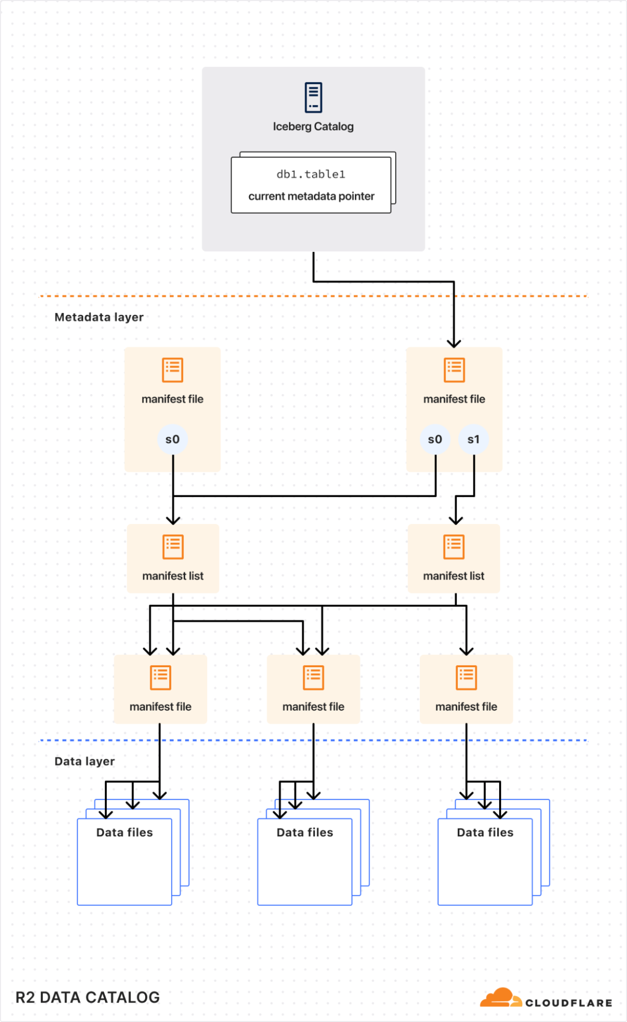
The technology that enables this is Apache Iceberg. Iceberg is a table format, which provides database-like capabilities (including updates, ACID transactions, and schema evolution) on top of data files in object storage. In other words, it’s a metadata layer that tells clients which data files make up a particular logical table, what the schemas are, and how to efficiently query them.

The adoption of Iceberg across the industry meant users were no longer locked-in to one query engine. But egress fees still make it cost-prohibitive to query data across regions and clouds. R2, with zero-cost egress, solves that problem — users would no longer be locked-in to their clouds either. They could store their data in a vendor-neutral location and let teams use whatever query engine made sense for their data and query patterns.

But users still had to manage all of the metadata and other infrastructure themselves. We realized there was an opportunity for us to solve a major pain point and reduce the friction of storing data lakes on R2. This became R2 Data Catalog, our managed Iceberg catalog.

With the data stored on R2 and metadata managed, that still left a few gaps for users to solve.

How do you get data into your Iceberg tables? Once it’s there, how do you optimize for query performance? And how do you actually get value from your data without needing to self-host a query engine or use another cloud platform?

In the rest of this post, we’ll walk through how the three products that make up the Data Platform solve these challenges.

Cloudflare Pipelines

Analytical data tables are made up of events, things that happened at a particular point in time. They might come from server logs, mobile applications, or IoT devices, and are encoded in data formats like JSON, Avro, or Protobuf. They ideally have a schema — a standardized set of fields — but might just be whatever a particular team thought to throw in there.

But before you can query your events with Iceberg, they need to be ingested, structured according to a schema, and written into object storage. This is the role of Cloudflare Pipelines.

Built on top of Arroyo, a stream processing engine we acquired earlier this year, Pipelines receives events, transforms them with SQL queries, and sinks them to R2 and R2 Data Catalog.

Pipelines is organized around three central objects:

Streams are how you get data into Cloudflare. They’re durable, buffered queues that receive events and store them for processing. Streams can accept events in two ways: via an HTTP endpoint or from a Cloudflare Worker binding.

Sinks define the destination for your data. We support ingesting into R2 Data Catalog, as well as writing raw files to R2 as JSON or Apache Parquet. Sinks can be configured to frequently write files, prioritizing low-latency ingestion, or to write less frequent, larger files to get better query performance. In either case, ingestion is exactly-once, which means that we will never duplicate or drop events on their way to R2.

Pipelines connect streams and sinks via SQL transformations, which can modify events before writing them to storage. This enables you to shift left, pushing validation, schematization, and processing to your ingestion layer to make your queries easy, fast, and correct.


For example, here’s a pipeline that ingests events from a clickstream data source and writes them to Iceberg:

INSERT into events_table
SELECT
  user_id,
  lower(event) AS event_type,
  to_timestamp_micros(ts_us) AS event_time,
  regexp_match(url, '^https?://([^/]+)')[1]  AS domain,
  url,
  referrer,
  user_agent
FROM events_json
WHERE event = 'page_view'
  AND NOT regexp_like(user_agent, '(?i)bot|spider');

SQL transformations are very powerful and give you full control over how data is structured and written into the table. For example, you can

  • Schematize and normalize your data, even using JSON functions to extract fields from arbitrary JSON

  • Filter out events or split them into separate tables with their own schemas

  • Redact sensitive information before storage with regexes

  • Unroll nested arrays and objects into separate events

Initially, Pipelines supports stateless transformations. In the future, we’ll leverage more of Arroyo’s stateful processing capabilities to support aggregations, incrementally-updated materialized views, and joins.

Cloudflare Pipelines is available today in open beta. You can create a pipeline using the dashboard, Wrangler, or the REST API. To get started, check out our developer docs.

We aren’t currently billing for Pipelines during the open beta. However, R2 storage and operations incurred by sinks writing data to R2 are billed at standard rates. When we start billing, we anticipate charging based on the amount of data read, the amount of data processed via SQL transformations, and data delivered.

R2 Data Catalog

We launched the open beta of R2 Data Catalog in April and have been amazed by the response. Query engines like DuckDB have added native support, and we’ve seen useful integrations like marimo notebooks.

It makes getting started with Iceberg easy. There’s no need to set up a database cluster, connect to object storage, or manage any infrastructure. You can create a catalog with a couple of Wrangler commands:

$ npx wrangler bucket create mycatalog 
$ npx wrangler r2 bucket catalog enable mycatalog

This provisions a data lake that can scale to petabytes of storage, queryable by whatever engine you want to use with zero egress fees.

But just storing the data isn’t enough. Over time, as data is ingested, the number of underlying data files that make up a table will grow, leading to slower and slower query performance.

This is a particular problem with low-latency ingestion, where the goal is to have events queryable as quickly as possible. Writing data frequently means the files are smaller, and there are more of them. Each file needed for a query has to be listed, downloaded, and read. The overhead of too many small files can dominate the total query time.

The solution is compaction, a periodic maintenance operation performed automatically by the catalog. Compaction rewrites small files into larger files which reduces metadata overhead and increases query performance. 

Today we are launching compaction support in R2 Data Catalog. Enabling it for your catalog is as easy as:

$ npx wrangler r2 bucket catalog compaction enable mycatalog

We’re starting with support for small-file compaction, and will expand to additional compaction strategies in the future. Check out the compaction documentation to learn more about how it works and how to enable it.

At this time, during open beta, we aren’t billing for R2 Data Catalog. Below is our current thinking on future pricing:

Pricing*

R2 storage

For standard storage class

$0.015 per GB-month (no change)

R2 Class A operations

$4.50 per million operations (no change)

R2 Class B operations

$0.36 per million operations (no change)

Data Catalog operations

e.g., create table, get table metadata, update table properties

$9.00 per million catalog operations

Data Catalog compaction data processed

$0.005 per GB processed

$2.00 per million objects processed

Data egress

$0 (no change, always free)

*prices subject to change prior to General Availability

We will provide at least 30 days notice before billing starts or if anything changes.

R2 SQL

Having data in R2 Data Catalog is only the first step; the real goal is getting insights and value from it. Traditionally, that means setting up and managing DuckDB, Spark, Trino, or another query engine, adding a layer of operational overhead between you and those insights. What if instead you could run queries directly on Cloudflare?

Now you can. We’ve built a query engine specifically designed for R2 Data Catalog and Cloudflare’s edge infrastructure. We call it R2 SQL, and it’s available today as an open beta.

With Wrangler, running a query on an R2 Data Catalog table is as easy as

$ npx wrangler r2 sql query "{WAREHOUSE}" "\
  SELECT user_id, url FROM events \
  WHERE domain = 'mywebsite.com'"

Cloudflare’s ability to schedule compute anywhere on its global network is the foundation of R2 SQL’s design. This lets us process data directly where it lives, instead of requiring you to manage centralized clusters for your analytical workloads.

R2 SQL is tightly integrated with R2 Data Catalog and R2, which allows the query planner to go beyond simple storage scanning and make deep use of the rich statistics stored in the R2 Data Catalog metadata. This provides a powerful foundation for a new class of query optimizations, such as auxiliary indexes or enabling more complex analytical functions in the future.

The result is a fully serverless experience for users. You can focus on your SQL without needing a deep understanding of how the engine operates. If you are interested in how R2 SQL works, the team has written a deep dive into how R2 SQL’s distributed query engine works at scale.

The open beta is an early preview of R2 SQL querying capabilities, and is initially focused around filter queries. Over time, we will be expanding its capabilities to cover more SQL features, like complex aggregations.

We’re excited to see what our users do with R2 SQL. To try it out, see the documentation and tutorials. During the beta, R2 SQL usage is not currently billed, but R2 storage and operations incurred by queries are billed at standard rates. We plan to charge for the volume of data scanned by queries in the future and will provide notice before billing begins.

Wrapping up

Today, you can use the Cloudflare Data Platform to ingest events into R2 Data Catalog and query them via R2 SQL. In the first half of 2026, we’ll be expanding on the capabilities in all of these products, including:

  • Integration with Logpush, so you can transform, store, and query your logs directly within Cloudflare

  • User-defined functions via Workers, and stateful processing support for streaming transformations

  • Expanding the featureset of R2 SQL to cover aggregations and joins

In the meantime, you can get started with the Cloudflare Data Platform by following the tutorial to create an end-to-end analytical data system, from ingestion with Pipelines, through storage in R2 Data Catalog, and querying with R2 SQL. 

We’re excited to see what you build! Come share your feedback with us on our Developer Discord.

Use Databricks Unity Catalog Open APIs for Spark workloads on Amazon EMR

Post Syndicated from Venkat Viswanathan original https://aws.amazon.com/blogs/big-data/use-databricks-unity-catalog-open-apis-for-spark-workloads-on-amazon-emr/

This post was written with John Spencer, Sreeram Thoom, and Dipankar Kushari from Databricks.

Organizations need seamless access to data across multiple platforms and business units. A common scenario involves one team using Amazon EMR for data processing while needing to access data that another team manages in Databricks Unity Catalog. Traditionally, this would require data duplication or complex manual setups.

Although both Amazon EMR and Databricks Unity Catalog are powerful tools on their own, integrating them effectively is crucial for maintaining strong data governance, security, and operational efficiency. In this post, we demonstrate how to achieve this integration using Amazon EMR Serverless, though the approach works well with other Amazon EMR deployment options and Unity Catalog OSS.

EMR Serverless makes running big data analytics frameworks straightforward by offering a serverless option that automatically provisions and manages the infrastructure required to run big data applications. Teams can run Apache Spark and other workloads without the complexity of cluster management, while providing cost-effective scaling based on actual workload demands and seamless integration with AWS services and security controls.

Databricks Unity Catalog serves as a unified governance solution for data and AI assets, providing centralized access control and auditing capabilities. It enables fine-grained permissions across workspaces and cloud platforms, while supporting comprehensive metadata management and data discovery across the organization, and can complement governance tools like AWS Lake Formation.

To enable Amazon EMR to process data maintained in Unity Catalog, the data team traditionally copies data products across the platforms to a location accessible by Amazon EMR. The practice of data duplication not only leads to increased storage costs, but also severely impacts data quality and makes it challenging to effectively enforce same governance policies across different systems, track data lineage, enforce data retention policies, and maintain consistent access controls across the organization.

Now using Unity Catalog’s Open REST APIs, Amazon EMR customers can read from and write to Databricks Unity Catalog and Unity Catalog OSS tables using Spark, enabling cross-platform interoperability while maintaining governance and access controls across Amazon EMR and Unity Catalog.

Solution overview

In this post, we will provide an overview of EMR Spark workload integration with Databricks Unity Catalog and walk through the end-to-end process of reading from and writing to Databricks Unity Catalog tables using Amazon EMR and Spark. We show you how to configure EMR Serverless to interact with Databricks Unity Catalog, run an interactive Spark workload to access the data, and run an analysis to derive insights.

The following diagram illustrates the solution architecture.

Prerequisites

You must have the following prerequisites:

In the following sections, we walk through the process of reading and writing to Unity Catalog with EMR Serverless.

Enable Unity Catalog for external access

Log in to your workspace as a Databricks admin and complete the following steps to configure external access to read Databricks objects:

  1. Enable external data access for your metastore. For instructions, see Enable external data access on the metastore.
  2. Set up a principal that will be configured with Amazon EMR for data access.
  3. Grant the principal the privilege to configure the integration of the EXTERNAL USE SCHEMA privilege on the schema containing the objects. For instructions, see Grant a principal EXTERNAL USE SCHEMA.
  4. For this post, we generate a Databricks personal access token (PAT) for the principal and note it down. For instructions, refer to Authorizing access to Databricks resources and Databricks personal access token authentication.

For a production deployment, store the PAT in AWS Secrets Manager. You can use it in a later step to read and write to Unity Catalog with Amazon EMR.

Configure EMR Spark to access Unity Catalog

In this walkthrough, we run PySpark interactive queries through notebooks using EMR Studio. Complete the following steps:

  1. Open the AWS Management Console with administrator permission.
  2. Create an EMR Studio to run interactive workloads. To create a workspace, you need to specify the S3 bucket created in the prerequisites and the minimum service role for EMR Serverless. For instructions, see Set up an EMR Studio.
  3. For this post, we create two EMR Serverless applications. For instructions, see Creating an EMR Serverless application from the EMR Studio console.
    1. For Iceberg tables, create an EMR Serverless application called dbx-demo-application-iceberg with version 7.8.0 or higher. Make sure to deselect Use AWS Glue Data Catalog as Metastore under Additional Configurations, Metastore configuration. Add the following Spark configuration (see Configure applications). Provide the name of the catalog in Unity Catalog that contains your tables and the URL of the Databricks workspace.
      {
          "runtimeConfiguration": [
              {
                  "classification": "spark-defaults",
                  "properties": {
                      "spark.jars": "/usr/share/aws/iceberg/lib/iceberg-spark3-runtime.jar",
                      "spark.jars.packages": "io.unitycatalog:unitycatalog-spark_2.12:0.2.0",
                      "spark.sql.extensions": "org.apache.iceberg.spark.extensions.IcebergSparkSessionExtensions",
                      "spark.sql.defaultCatalog": "<uc-catalog-name>",
                      "spark.sql.catalog.<uc-catalog-name>": "org.apache.iceberg.spark.SparkCatalog",
                      "spark.sql.catalog.<uc-catalog-name>.uri": "https://<workspace-url>/api/2.1/unity-catalog/iceberg-rest",
                      "spark.sql.catalog.<uc-catalog-name>.type": "rest",
                      "spark.sql.catalog.<uc-catalog-name>.warehouse": "<uc-catalog-name>"
                  }
              }
          ]
      }

    2. For Delta tables, create an EMR Serverless application called dbx-demo-application and version 7.8.0 or higher. Make sure to deselect Use AWS Glue Data Catalog as Metastore under Additional Configurations, Metastore configuration. Add the following Spark configuration (see Configure applications). Provide the name of the catalog in Unity Catalog that contains your tables and the URL of the Databricks workspace.
      {
          "runtimeConfiguration": [
              {
                  "classification": "spark-defaults",
                  "properties": {
                      "spark.jars": "/usr/share/aws/delta/lib/delta-spark.jar,/usr/share/aws/delta/lib/delta- storage.jar",
                      "spark.jars.packages": "io.unitycatalog:unitycatalog-spark_2.12:0.2.0",
                      "spark.sql.extensions": "io.delta.sql.DeltaSparkSessionExtension",
                      "spark.sql.defaultCatalog": "<uc-catalog-name>",
                      "spark.sql.catalog.spark_catalog": "io.unitycatalog.spark.UCSingleCatalog",
                      "spark.sql.catalog.<uc-catalog-name>": "io.unitycatalog.spark.UCSingleCatalog",
                      "spark.sql.catalog.<uc-catalog-name>.uri": "https://<workspace-url>/api/2.1/unity-catalog"
                  }
              }
          ]
      }

  4. To set up your interactive workload with a runtime role, see Run interactive workloads with EMR Serverless through EMR Studio.

Read and write to Unity Catalog with Amazon EMR

Launch the workspace created in the previous step. Download the notebooks create-delta-table and create-iceberg-table and upload them to the EMR Studio workspace.

The create-delta-table.ipynb notebook configures the metastore properties to work with Delta tables. The create-iceberg-table.ipynb notebook configures the metastore properties to work with Iceberg tables.

Add the generated token to the session.

For a production deployment, store the PAT in Secrets Manager.

For Iceberg tables, connect to the EMR Serverless application dbx-demo-application-iceberg with the runtime role created in earlier steps under compute and run the notebook (create-iceberg-table). Select PySpark as the kernel and execute each cell in the notebook by choosing the run icon. Refer to Submit a job run or interactive workload for further details about how to run an interactive notebook.

We use the following code to create an external Iceberg table in the catalog:

CREATE SCHEMA IF NOT EXISTS customerschema;
USE SCHEMA customerschema;
CREATE TABLE IF NOT EXISTS iceberg_customer (id string, name string, country string) USING iceberg; 
insert into iceberg customer values('1','Alice','US');

For Delta tables, connect to the EMR Serverless application dbx-demo-application with the runtime role created in earlier steps and run the notebook (create-delta-table). Select PySpark as the kernel and execute each cell in the notebook by choosing the run icon. Refer to Submit a job run or interactive workload for further details about how to run an interactive notebook.

We use the following code to create an external Delta table in the catalog:

CREATE SCHEMA IF NOT EXISTS customerschema;
USE SCHEMA customerschema;
CREATE TABLE IF NOT EXISTS delta_customer (id int, name string, country string) USING delta LOCATION ‘s3://<bucket_name>/emr-dbx/external/customerschema/delta_customer’;
insert into delta_customer values(1,'Bob','US'); 

Verify in Databricks for both Iceberg and Delta tables

Now you can run queries in Databricks Unity Catalog to show the records inserted into the Iceberg and Delta tables from EMR Serverless:

  1. Log in to your Databricks workspace.
  2. Choose SQL Editor in the navigation pane.
  3. Run queries for both Iceberg and Delta tables.
  4. Verify the results show the same as what you saw in the Jupyter notebook in EMR Studio.

The following screenshot shows an example of querying the Iceberg table.

The following screenshot shows an example of querying the Delta table.

Clean up

Clean up the resources used in this post to avoid additional charges:

  1. Delete the IAM roles for this post.
  2. Delete the EMR applications and EMR Studio setup created for this post.
  3. Delete the resources created in Unity Catalog.
  4. Empty and then delete the S3 bucket.

Summary

In this post, we demonstrated the powerful interoperability between Amazon EMR and Databricks Unity Catalog by walking through how to enable external access to Unity Catalog, configure EMR Spark to connect seamlessly with Unity Catalog, and perform DML and DDL operations on Unity Catalog tables using EMR Serverless.

To learn more about using EMR Serverless, see Getting started with Amazon EMR Serverless. To learn more about using tools like EMR Spark with Unity Catalog, see Unity Catalog integrations.


About the authors

Venkatavaradhan (Venkat) Viswanathan is a Global Partner Solutions Architect at Amazon Web Services. Venkat is a Technology Strategy Leader in Data, AI, ML, generative AI, and Advanced Analytics. Venkat is a Global SME for Databricks and helps AWS customers design, build, secure, and optimize Databricks workloads on AWS.

Srividya Parthasarathy is a Senior Big Data Architect on the AWS Lake Formation team. She works with the product team and customers to build robust features and solutions for their analytical data platform. She enjoys building data mesh solutions and sharing them with the community.

Ramkumar Nottath is a Principal Solutions Architect at AWS focusing on Analytics services. He enjoys working with various customers to help them build scalable, reliable big data and analytics solutions. His interests extend to various technologies such as analytics, data warehousing, streaming, data governance, and machine learning. He loves spending time with his family and friends.

John Spencer is a Product Manager at Databricks, dedicated to making Unity Catalog work seamlessly with customers’ ecosystems of tools and platforms so they can easily access, govern, and use their data.

Sreeram Thoom is a Specialist Solutions Architect at Databricks helping customers design secure, scalable applications on the Data Lakehouse.

Dipankar Kushari is a specialist solutions architect at Databricks helping customer architect and build secured applications on Data Lakehouse.

Explore your Cloudflare data with Python notebooks, powered by marimo

Post Syndicated from Carlos Rodrigues original https://blog.cloudflare.com/marimo-cloudflare-notebooks/

Many developers, data scientists, and researchers do much of their work in Python notebooks: they’ve been the de facto standard for data science and sharing for well over a decade. Notebooks are popular because they make it easy to code, explore data, prototype ideas, and share results. We use them heavily at Cloudflare, and we’re seeing more and more developers use notebooks to work with data – from analyzing trends in HTTP traffic, querying Workers Analytics Engine through to querying their own Iceberg tables stored in R2.

Traditional notebooks are incredibly powerful — but they were not built with collaboration, reproducibility, or deployment as data apps in mind. As usage grows across teams and workflows, these limitations face the reality of work at scale.

marimo reimagines the notebook experience with these challenges in mind. It’s an open-source reactive Python notebook that’s built to be reproducible, easy to track in Git, executable as a standalone script, and deployable. We have partnered with the marimo team to bring this streamlined, production-friendly experience to Cloudflare developers. Spend less time wrestling with tools and more time exploring your data.

Today, we’re excited to announce three things:

Want to start exploring your Cloudflare data with marimo right now? Head over to notebooks.cloudflare.com. Or, keep reading to learn more about marimo, how we’ve made authentication easy from within notebooks, and how you can use marimo to explore and share notebooks and apps on Cloudflare.

Why marimo?

marimo is an open-source reactive Python notebook designed specifically for working with data, built from the ground up to solve many problems with traditional notebooks.

The core feature that sets marimo apart from traditional notebooks is its reactive execution model, powered by a statically inferred dataflow graph on cells. Run a cell or interact with a UI element, and marimo either runs dependent cells or marks them as stale (your choice). This keeps code and outputs consistent, prevents bugs before they happen, and dramatically increases the speed at which you can experiment with data. 

Thanks to reactive execution, notebooks are also deployable as data applications, making them easy to share. While you can run marimo notebooks locally, on cloud servers, GPUs — anywhere you can traditionally run software — you can also run them entirely in the browser with WebAssembly, bringing the cost of sharing down to zero.

Because marimo notebooks are stored as Python, they enjoy all the benefits of software: version with Git, execute as a script or pipeline, test with pytest, inline package requirements with uv, and import symbols from your notebook into other Python modules. Though stored as Python, marimo also supports SQL and data sources like DuckDB, Postgres, and Iceberg-based data catalogs (which marimo’s AI assistant can access, in addition to data in RAM).

To get an idea of what a marimo notebook is like, check out the embedded example notebook below:

Exploring your Cloudflare data with marimo

Ready to explore your own Cloudflare data in a marimo notebook? The easiest way to begin is to visit notebooks.cloudflare.com and run one of our example notebooks directly in your browser via WebAssembly (Wasm). You can also browse the source in our notebook examples GitHub repo.

Want to create your own notebook to run locally instead? Here’s a quick example that shows you how to authenticate with your Cloudflare account and list the zones you have access to:

  1. Install uv if you haven’t already by following the installation guide.

  2. Create a new project directory for your notebook:

mkdir cloudflare-zones-notebook
cd cloudflare-zones-notebook

3. Initialize a new uv project (this creates a .venv and a pyproject.toml):

uv init

4. Add marimo and required dependencies:

uv add marimo

5. Create a file called list-zones.py and paste in the following notebook:

import marimo

__generated_with = "0.14.10"
app = marimo.App(width="full", auto_download=["ipynb", "html"])


@app.cell
def _():
    from moutils.oauth import PKCEFlow
    import requests

    # Start OAuth PKCE flow to authenticate with Cloudflare
    auth = PKCEFlow(provider="cloudflare")

    # Renders login UI in notebook
    auth
    return (auth,)


@app.cell
def _(auth):
    import marimo as mo
    from cloudflare import Cloudflare

    mo.stop(not auth.access_token, mo.md("Please **sign in** using the button above."))
    client = Cloudflare(api_token=auth.access_token)

    zones = client.zones.list()
    [zone.name for zone in zones.result]
    return


if __name__ == "__main__":
    app.run()

6. Open the notebook editor:

uv run marimo edit list-zones.py --sandbox

7. Log in via the OAuth prompt in the notebook. Once authenticated, you’ll see a list of your Cloudflare zones in the final cell.

That’s it! From here, you can expand the notebook to call Workers AI models, query Iceberg tables in R2 Data Catalog, or interact with any Cloudflare API.

How OAuth works in notebooks

Think of OAuth like a secure handshake between your notebook and Cloudflare. Instead of copying and pasting API tokens, you just click “Sign in with Cloudflare” and the notebook handles the rest.

We built this experience using PKCE (Proof Key for Code Exchange), a secure OAuth 2.0 flow that avoids client secrets and protects against code interception attacks. PKCE works by generating a one-time code that’s exchanged for a token after login, without ever sharing a client secret. Learn more about how PKCE works.

The login widget lives in moutils.oauth, a collaboration between Cloudflare and marimo to make OAuth authentication simple and secure in notebooks. To use it, just create a cell like this:

auth = PKCEFlow(provider="cloudflare")

# Renders login UI in notebook
auth

When you run the cell, you’ll see a Sign in with Cloudflare button:


Once logged in, you’ll have a read-only access token you can pass when using the Cloudflare API.

Running marimo on Cloudflare: Workers and Containers

In addition to running marimo notebooks locally, you can use Cloudflare to share and run them via Workers Static Assets or Cloudflare Containers.

If you have a local notebook you want to share, you can publish it to Workers. This works because marimo can export notebooks to WebAssembly, allowing them to run entirely in the browser. You can get started with just two commands:

marimo export html-wasm notebook.py -o output_dir --mode edit --include-cloudflare
npx wrangler deploy

If your notebook needs authentication, you can layer in Cloudflare Access for secure, authenticated access.

For notebooks that require more compute, persistent sessions, or long-running tasks, you can deploy marimo on our new container platform. To get started, check out our marimo container example on GitHub.

What’s next for Cloudflare + marimo

This blog post marks just the beginning of Cloudflare’s partnership with marimo. While we’re excited to see how you use our joint WebAssembly-based notebook platform to explore your Cloudflare data, we also want to help you bring serious compute to bear on your data — to empower you to run large scale analyses and batch jobs straight from marimo notebooks. Stay tuned!

Model Once, Represent Everywhere: UDA (Unified Data Architecture) at Netflix

Post Syndicated from Netflix Technology Blog original https://netflixtechblog.com/uda-unified-data-architecture-6a6aee261d8d

By Alex Hutter, Alexandre Bertails, Claire Wang, Haoyuan He, Kishore Banala, Peter Royal, Shervin Afshar

As Netflix’s offerings grow — across films, series, games, live events, and ads — so does the complexity of the systems that support it. Core business concepts like ‘actor’ or ‘movie’ are modeled in many places: in our Enterprise GraphQL Gateway powering internal apps, in our asset management platform storing media assets, in our media computing platform that powers encoding pipelines, to name a few. Each system models these concepts differently and in isolation, with little coordination or shared understanding. While they often operate on the same concepts, these systems remain largely unaware of that fact, and of each other.

Spider-Man Pointing meme with each Spider-Man labelled as: “it’s a movie”, “it’s a tv show”, “it’s a game”.

As a result, several challenges emerge:

  • Duplicated and Inconsistent Models — Teams re-model the same business entities in different systems, leading to conflicting definitions that are hard to reconcile.
  • Inconsistent Terminology — Even within a single system, teams may use different terms for the same concept, or the same term for different concepts, making collaboration harder.
  • Data Quality Issues — Discrepancies and broken references are hard to detect across our many microservices. While identifiers and foreign keys exist, they are inconsistently modeled and poorly documented, requiring manual work from domain experts to find and fix any data issues.
  • Limited Connectivity — Within systems, relationships between data are constrained by what each system supports. Across systems, they are effectively non-existent.

To address these challenges, we need new foundations that allow us to define a model once, at the conceptual level, and reuse those definitions everywhere. But it isn’t enough to just document concepts; we need to connect them to real systems and data. And more than just connect, we have to project those definitions outward, generating schemas and enforcing consistency across systems. The conceptual model must become part of the control plane.

These were the core ideas that led us to build UDA.

Introducing UDA

UDA (Unified Data Architecture) is the foundation for connected data in Content Engineering. It enables teams to model domains once and represent them consistently across systems — powering automation, discoverability, and semantic interoperability.

Using UDA, users and systems can:

Register and connect domain models — formal conceptualizations of federated business domains expressed as data.

  • Why? So everyone uses the same official definitions for business concepts, which avoids confusion and stops different teams from rebuilding similar models in conflicting ways.

Catalog and map domain models to data containers, such as GraphQL type resolvers served by a Domain Graph Service, Data Mesh sources, or Iceberg tables, through their representation as a graph.

  • Why? To make it easy to find where the actual data for these business concepts lives (e.g., in which specific database, table, or service) and understand how it’s structured there.

Transpile domain models into schema definition languages like GraphQL, Avro, SQL, RDF, and Java, while preserving semantics.

  • Why? To automatically create consistent technical data structures (schemas) for various systems directly from the domain models, saving developers manual effort and reducing errors caused by out-of-sync definitions.

Move data faithfully between data containers, such as from federated GraphQL entities to Data Mesh (a general purpose data movement and processing platform for moving data between Netflix systems at scale), Change Data Capture (CDC) sources to joinable Iceberg Data Products.

  • Why? To save developer time by automatically handling how data is moved and correctly transformed between different systems. This means less manual work to configure data movement, ensuring data shows up consistently and accurately wherever it’s needed.

Discover and explore domain concepts via search and graph traversal.

  • Why? So anyone can more easily find the specific business information they’re looking for, understand how different concepts and data are related, and be confident they are accessing the correct information.

Programmatically introspect the knowledge graph using Java, GraphQL, or SPARQL.

  • Why? So developers can build smarter applications that leverage this connected business information, automate more complex data-dependent workflows, and help uncover new insights from the relationships in the data.

This post introduces the foundations of UDA as a knowledge graph, connecting domain models to data containers through mappings, and grounded in an in-house metamodel, or model of models, called Upper. Upper defines the language for domain modeling in UDA and enables projections that automatically generate schemas and pipelines across systems.

Image of the UDA knowledge graph. A central node representing a domain model is connected to other nodes representing Data Mesh, GraphQL, and Iceberg data containers.
The same domain model can be connected to semantically equivalent data containers in the UDA knowledge graph.

This post also highlights two systems that leverage UDA in production:

Primary Data Management (PDM) is our platform for managing authoritative reference data and taxonomies. PDM turns domain models into flat or hierarchical taxonomies that drive a generated UI for business users. These taxonomy models are projected into Avro and GraphQL schemas, automatically provisioning data products in the Warehouse and GraphQL APIs in the Enterprise Gateway.

Sphere is our self-service operational reporting tool for business users. Sphere uses UDA to catalog and relate business concepts across systems, enabling discovery through familiar terms like ‘actor’ or ‘movie.’ Once concepts are selected, Sphere walks the knowledge graph and generates SQL queries to retrieve data from the warehouse, no manual joins or technical mediation required.

UDA is a Knowledge Graph

UDA needs to solve the data integration problem. We needed a data catalog unified with a schema registry, but with a hard requirement for semantic integration. Connecting business concepts to schemas and data containers in a graph-like structure, grounded in strong semantic foundations, naturally led us to consider a knowledge graph approach.

We chose RDF and SHACL as the foundation for UDA’s knowledge graph. But operationalizing them at enterprise scale surfaced several challenges:

  • RDF lacked a usable information model. While RDF offers a flexible graph structure, it provides little guidance on how to organize data into named graphs, manage ontology ownership, or define governance boundaries. Standard follow-your-nose mechanisms like owl:imports apply only to ontologies and don’t extend to named graphs; we needed a generalized mechanism to express and resolve dependencies between them.
  • SHACL is not a modeling language for enterprise data. Designed to validate native RDF, SHACL assumes globally unique URIs and a single data graph. But enterprise data is structured around local schemas and typed keys, as in GraphQL, Avro, or SQL. SHACL could not express these patterns, making it difficult to model and validate real-world data across heterogeneous systems.
  • Teams lacked shared authoring practices. Without strong guidelines, teams modeled their ontologies inconsistently breaking semantic interoperability. Even subtle differences in style, structure, or naming led to divergent interpretations and made transpilation harder to define consistently across schemas.
  • Ontology tooling lacked support for collaborative modeling. Unlike GraphQL Federation, ontology frameworks had no built-in support for modular contributions, team ownership, or safe federation. Most engineers found the tools and concepts unfamiliar, and available authoring environments lacked the structure needed for coordinated contributions.

To address these challenges, UDA adopts a named-graph-first information model. Each named graph conforms to a governing model, itself a named graph in the knowledge graph. This systematic approach ensures resolution, modularity, and enables governance across the entire graph. While a full description of UDA’s information infrastructure is beyond the scope of this post, the next sections explain how UDA bootstraps the knowledge graph with its metamodel and uses it to model data container representations and mappings.

Upper is Domain Modeling

Upper is a language for formally describing domains — business or system — and their concepts. These concepts are organized into domain models: controlled vocabularies that define classes of keyed entities, their attributes, and their relationships to other entities, which may be keyed or nested, within the same domain or across domains. Keyed concepts within a domain model can be organized in taxonomies of types, which can be as complex as the business or the data system needs them to be. Keyed concepts can also be extended from other domain models — that is, new attributes and relationships can be contributed monotonically. Finally, Upper ships with a rich set of datatypes for attribute values, which can also be customized per domain.

Visualization of the UDA graph representation of a One Piece character. The Character node in the graph is connected to a Devil Fruit node. The Devil Fruit node is connected to a Devil Fruit Type node.
The graph representation of the onepiece: domain model from our UI. Depicted here you can see how Characters are related to Devil Fruit, and that each Devil Fruit has a type.

Upper domain models are data. They are expressed as conceptual RDF and organized into named graphs, making them introspectable, queryable, and versionable within the UDA knowledge graph. This graph unifies not just the domain models themselves, but also the schemas they transpile to — GraphQL, Avro, Iceberg, Java — and the mappings that connect domain concepts to concrete data containers, such as GraphQL type resolvers served by a Domain Graph Service, Data Mesh sources, or Iceberg tables, through their representations. Upper raises the level of abstraction above traditional ontology languages: it defines a strict subset of semantic technologies from the W3C tailored and generalized for domain modeling. It builds on ontology frameworks like RDFS, OWL, and SHACL so domain authors can model effectively without even needing to learn what an ontology is.

Screenshot of UDA UI showing domain model for One Piece serialized as Turtle.
UDA domain model for One Piece. Link to full definition.

Upper is the metamodel for Connected Data in UDA — the model for all models. It is designed as a bootstrapping upper ontology, which means that Upper is self-referencing, because it models itself as a domain model; self-describing, because it defines the very concept of a domain model; and self-validating, because it conforms to its own model. This approach enables UDA to bootstrap its own infrastructure: Upper itself is projected into a generated Jena-based Java API and GraphQL schema used in GraphQL service federated into Netflix’s Enterprise GraphQL gateway. These same generated APIs are then used by the projections and the UI. Because all domain models are conservative extensions of Upper, other system domain models — including those for GraphQL, Avro, Data Mesh, and Mappings — integrate seamlessly into the same runtime, enabling consistent data semantics and interoperability across schemas.

Screenshot of an IDE. It shows Java code using the generated API from the Upper metamodel to traverse and print terms from a domain domain in the top while the bottom contains the output of an execution.
Traversing a domain model programmatically using the Java API generated from the Upper metamodel.

Data Container Representations

Data containers are repositories of information. They contain instance data that conform to their own schema languages or type systems: federated entities from GraphQL services, Avro records from Data Mesh sources, rows from Iceberg tables, or objects from Java APIs. Each container operates within the context of a system that imposes its own structural and operational constraints.

Screenshot of a UI showing details for a Data Mesh Source containing One Piece Characters.
A Data Mesh source is a data container.

Data container representations are data. They are faithful interpretations of the members of data systems as graph data. UDA captures the definition of these systems as their own domain models, the system domains. These models encode both the information architecture of the systems and the schemas of the data containers within. They provide a blueprint for translating the systems into graph representations.

Screenshot of an IDE showing two files open side by side. On the left is a system domain model for Data Mesh. On the right is a representation of a Data Mesh source containing One Piece Character data.
Side by side/super imposed image of data container schema and representation. Link to full data container representation.

UDA catalogs the data container representations into the knowledge graph. It records the coordinates and metadata of the underlying data assets, but unlike a traditional catalog, it only tracks assets that are semantically connected to domain models. This enables users and systems to connect concepts from domain models to the concrete locations where corresponding instance data can be accessed. Those connections are called Mappings.

Mappings

Mappings are data that connect domain models to data containers. Every element in a domain model is addressable, from the domain model itself down to specific attributes and relationships. Likewise, data container representations make all components addressable, from an Iceberg table to an individual column, or from a GraphQL type to a specific field. A Mapping connects nodes in a subgraph of the domain model to nodes in a subgraph of a container representation. Visually, the Mapping is the set of arcs that link those two graphs together.

Screenshot of UDA UI showing a mapping between a concept in UDA and a Data Mesh Source.
A mapping between a domain model and a Data Mesh Source from the UDA UI. Link to full mapping.

Mappings enable discovery. Starting from a domain concept, users and systems can walk the knowledge graph to find where that concept is materialized — in which data system, in which container, and even how a specific attribute or relationship is physically accessed. The inverse is also supported: given a data container, one can trace back to the domain concepts it participates in.

Mappings shape UDA’s approach to semantic data integration. Most existing schema languages are not expressive enough in capturing richer semantics of a domain to address requirements for data integration (for example, “accessibility of data, providing semantic context to support its interpretation, and establishing meaningful links between data”). A trivial example of this could be seen in the lack of built-in facilities in Avro to represent foreign keys, making it very hard to express how entities relate across Data Mesh sources. Mappings, together with the corresponding system domain models, allow for such relationships, and many other constraints, to be defined in the domain models and used programmatically in actual data systems.

Mappings enable intent-based automation. Data is not always available in the systems where consumers need it. Because Mappings encode both meaning and location, UDA can reason about how data should move, preserving semantics, without requiring the consumer to specify how it should be done. Beyond the cataloging use case, connecting to existing containers, UDA automatically derives canonical Mappings from registered domain models as part of the projection process.

Projections

A projection produces a concrete data container. These containers, such as a GraphQL schema or a Data Mesh source, implement the characteristics derived from a registered domain model. Each projection is a concrete realization of Upper’s denotational semantics, ensuring semantic interoperability across all containers projected from the same domain model.

Projections produce consistent public contracts across systems. The data containers generated by projections encode data contracts in the form of schemas, derived by transpiling a domain model into the target container’s schema language. UDA currently supports transpilation to GraphQL and Avro schemas.

The GraphQL transpilation produces a schema that adheres to the official GraphQL spec with the ability to generate all GraphQL types defined in the spec. Given that the UDA domain model can be federated, it also supports generating federated graphQL schemas. Below is an example of a transpiled GraphQL schema.

Screenshot of an IDE showing two files open side by side. On the left is the definition of a Character in UDA. On the right is transpiled GraphQL schema.
Domain model on the left, with transpiled GraphQL schema on the right. Link to full transpiled GraphQL schema.

The Avro transpilation produces a schema that is a Data Mesh flavor of Avro, which includes some customization on top of the official Avro spec. This schema is used to automatically create a Data Mesh source container. Below is an example of a transpiled Avro schema.

Screenshot of an IDE showing two files open side by side. On the left is the definition of a Devil Fruit in UDA. On the right is transpiled Avro schema.
Domain model on the left, with transpiled Avro schema on the right. Link to full transpiled Avro schema.

Projections can automatically populate data containers. Some projections, such as those to GraphQL schemas or Data Mesh sources produce empty containers that require developers to populate the data. This might be creating GraphQL APIs or pushing events onto Data Mesh sources. Conversely, other containers, like Iceberg Tables, are automatically created and populated by UDA. For Iceberg Tables, UDA leverages the Data Mesh platform to automatically create data streams to move data into tables. This process utilizes much of the same infrastructure detailed in this blog post here.

Projections have mappings. UDA automatically generates and manages mappings between the newly created data containers and the projected domain model.

Early Adopters

Controlled Vocabularies (PDM)

The full range of Netflix’s business activities relies on a sprawling data model that captures the details of our many business processes. Teams need to be able to coordinate operational activities to ensure that content production is complete, advertising campaigns are in place, and promotional assets are ready to deploy. We implicitly depend upon a singular definition of shared concepts, such as content production is complete. Multiple definitions create coordination challenges. Software (and humans) don’t know that the definitions mean the same thing.

We started the Primary Data Management (PDM) initiative to create unified and consistent definitions for the core concepts in our data model. These definitions form controlled vocabularies, standardized and governed lists for what values are permitted within certain fields in our data model.

Primary Data Management (PDM) is a single place where business users can manage controlled vocabularies. Our data model governance has been scattered across different tools and teams creating coordination challenges. This is an information management problem relating to the definition, maintenance and consistent use of reference data and taxonomies. This problem is not unique to Netflix, so we looked outward for existing solutions to this problem.

Screenshot of PDM UI
Managing the taxonomy of One Piece characters in PDM.

PDM uses the Simple Knowledge Organization System (SKOS) model. It is a W3C data standard designed for modeling knowledge. Its terminology is abstract, with Concepts that can be organized into ConceptSchemes and properties to describe various types of relationships. Every system is hardcoded against something, that’s how software knows how to manipulate data. We want a system that can work with a data model as its input, so we still need something concrete to build the software against. This is what SKOS provides, a generic basis for modeling knowledge that our system can understand.

PDM uses Domain Models to integrate SKOS into the rest of Content Engineering’s ecosystem. A core premise of the system is that it takes a domain model as input, and everything that can be derived is derived from that model. PDM builds a user interface based upon the model definition and leverages UDA to project this model into type-safe interfaces for other systems to use. The system will provision a Domain Graph Service (DGS) within our federated GraphQL API environment using a GraphQL schema that UDA projects from the domain model. UDA is also used to provision data movement pipelines which are able to feed our GraphSearch infrastructure as well as move data into the warehouse. The data movement systems use Avro schemas, and UDA creates a projection from the domain model to Avro.

Consumers of controlled vocabularies never know they’re using SKOS. Domain models use terms that fit in with the domain. SKOS’s generic notion of broader and narrower to define a hierarchy are hidden from consumers as super-properties within the model. This allows consumers to work with language that is familiar to them while enabling PDM to work with any model. The best of both worlds.

Operational Reporting (Sphere)

Operational reporting serves the detailed day-to-day activities and processes of a business domain. It is a reporting paradigm specialized in covering high-resolution, low-latency data sets.

Operational reporting systems should generate reports without relying on technical intermediaries. Operational reporting systems need to address the persistent challenge of empowering business users to explore and obtain the data they need, when they need it. Without such self-service systems, requests for new reports or data extracts often result in back-and-forth exchanges, where the initial query may not exactly meet business users’ expectations, requiring further clarification and refinement.

Data discovery and query generation are two relevant aspects of data integration. Supplying end-users with an accurate, contextual, and user-friendly data discovery experience provides a basis for query generation mechanism which produces syntactically correct and semantically reliable queries.

Operational reports are predominantly run on data hydrated from GraphQL services into the Data Warehouse. You can read about our journey from conventional data movement to streaming data pipelines based on CDC and GraphQL hydration in this blog post. Among the challenging byproducts of this approach was that a single, distinct data concept is now present in two places (GraphQL and data warehouse), with some disparity in semantic context to guide and support the interpretations and connectivity of that data. To address this, we formulate a mechanism to use the syntax and semantics captured in the federated schema from Netflix’s Enterprise GraphQL and populate representational domain models in UDA to preserve those details and add more.

Domain models enable the data discovery experience. Metadata aggregated from various data-producing systems is captured in UDA domain models using a unified vocabulary. This metadata is surfaced for the users’ search and discovery needs; instead of specifying exact tables and join keys, users simply can search for familiar business concepts such as ‘actors’ or ‘movies’. We use UDA models to disambiguate and resolve the intended concepts and their related data entities.

UDA knowledge graph is the data landscape for query generation. Once concepts are discovered and their mappings to corresponding data containers are identified and located in the knowledge graph, we use them to establish join strategies. Through graph traversal, we identify boundaries and islands within the data landscape. This ensures only feasible, joinable combinations are selected while weeding out semantically incorrect and non-executable query candidates.

Screenshot of Sphere’s UI
Generating a report in Sphere.

Sphere is a UDA-powered self-service operational reporting system. The solution based on knowledge graphs described above is called Sphere. Seeing self-service operational reporting through this lens, we can improve business users’ agency in access to operational data. They are empowered to explore, assemble, and refine reports at the conceptual level, while technical complexities are managed by the system.

Stay Tuned

UDA marks a fundamental shift in how we approach data modeling within Content Engineering. By providing a unified knowledge graph composed of what we know about our various data systems and the business concepts within them, we’ve made information more consistent, connected, and discoverable across our organization. We’re excited about future applications of these ideas such as:

  • Supporting additional projections like Protobuf/gRPC
  • Materializing the knowledge graph of instance data for querying, profiling, and management
  • Finally solving some of the initial challenges posed by Graph Search (that actually inspired some of this work)

If you’re interested in this space, we’d love to connect — whether you’re exploring new roles down the road or just want to swap ideas.

Expect to see future blog posts exploring PDM and Sphere in more detail soon!

Credits

Thanks to Andreas Legenbauer, Bernardo Gomez Palacio Valdes, Charles Zhao, Christopher Chong, Deepa Krishnan, George Pesmazoglou, Jessica Silva, Katherine Anderson, Malik Day, Rita Bogdanova, Ruoyun Zheng, Shawn Stedman, Suchita Goyal, Utkarsh Shrivastava, Yoomi Koh, Yulia Shmeleva


Model Once, Represent Everywhere: UDA (Unified Data Architecture) at Netflix was originally published in Netflix TechBlog on Medium, where people are continuing the conversation by highlighting and responding to this story.

R2 Data Catalog: Managed Apache Iceberg tables with zero egress fees

Post Syndicated from Phillip Jones original https://blog.cloudflare.com/r2-data-catalog-public-beta/

Apache Iceberg is quickly becoming the standard table format for querying large analytic datasets in object storage. We’re seeing this trend firsthand as more and more developers and data teams adopt Iceberg on Cloudflare R2. But until now, using Iceberg with R2 meant managing additional infrastructure or relying on external data catalogs.

So we’re fixing this. Today, we’re launching the R2 Data Catalog in open beta, a managed Apache Iceberg catalog built directly into your Cloudflare R2 bucket.

If you’re not already familiar with it, Iceberg is an open table format built for large-scale analytics on datasets stored in object storage. With R2 Data Catalog, you get the database-like capabilities Iceberg is known for – ACID transactions, schema evolution, and efficient querying – without the overhead of managing your own external catalog.

R2 Data Catalog exposes a standard Iceberg REST catalog interface, so you can connect the engines you already use, like PyIceberg, Snowflake, and Spark. And, as always with R2, there are no egress fees, meaning that no matter which cloud or region your data is consumed from, you won’t have to worry about growing data transfer costs.

Ready to query data in R2 right now? Jump into the developer docs and enable a data catalog on your R2 bucket in just a few clicks. Or keep reading to learn more about Iceberg, data catalogs, how metadata files work under the hood, and how to create your first Iceberg table.

What is Apache Iceberg?

Apache Iceberg is an open table format for analyzing large datasets in object storage. It brings database-like features – ACID transactions, time travel, and schema evolution – to files stored in formats like Parquet or ORC.

Historically, data lakes were just collections of raw files in object storage. However, without a unified metadata layer, datasets could easily become corrupted, were difficult to evolve, and queries often required expensive full-table scans.

Iceberg solves these problems by:

  • Providing ACID transactions for reliable, concurrent reads and writes.

  • Maintaining optimized metadata, so engines can skip irrelevant files and avoid unnecessary full-table scans.

  • Supporting schema evolution, allowing columns to be added, renamed, or dropped without rewriting existing data.

Iceberg is already widely supported by engines like Apache Spark, Trino, Snowflake, DuckDB, and ClickHouse, with a fast-growing community behind it.

How Iceberg tables are stored


Internally, an Iceberg table is a collection of data files (typically stored in columnar formats like Parquet or ORC) and metadata files (typically stored in JSON or Avro) that describe table snapshots, schemas, and partition layouts.

To understand how query engines interact efficiently with Iceberg tables, it helps to look at an Iceberg metadata file (simplified):

{
  "format-version": 2,
  "table-uuid": "0195e49b-8f7c-7933-8b43-d2902c72720a",
  "location": "s3://my-bucket/warehouse/0195e49b-79ca/table",
  "current-schema-id": 0,
  "schemas": [
    {
      "schema-id": 0,
      "type": "struct",
      "fields": [
        { "id": 1, "name": "id", "required": false, "type": "long" },
        { "id": 2, "name": "data", "required": false, "type": "string" }
      ]
    }
  ],
  "current-snapshot-id": 3567362634015106507,
  "snapshots": [
    {
      "snapshot-id": 3567362634015106507,
      "sequence-number": 1,
      "timestamp-ms": 1743297158403,
      "manifest-list": "s3://my-bucket/warehouse/0195e49b-79ca/table/metadata/snap-3567362634015106507-0.avro",
      "summary": {},
      "schema-id": 0
    }
  ],
  "partition-specs": [{ "spec-id": 0, "fields": [] }]
}

A few of the important components are:

  • schemas: Iceberg tracks schema changes over time. Engines use schema information to safely read and write data without needing to rewrite underlying files.

  • snapshots: Each snapshot references a specific set of data files that represent the state of the table at a point in time. This enables features like time travel.

  • partition-specs: These define how the table is logically partitioned. Query engines leverage this information during planning to skip unnecessary partitions, greatly improving query performance.

By reading Iceberg metadata, query engines can efficiently prune partitions, load only the relevant snapshots, and fetch only the data files it needs, resulting in faster queries.

Why do you need a data catalog?

Although the Iceberg data and metadata files themselves live directly in object storage (like R2), the list of tables and pointers to the current metadata need to be tracked centrally by a data catalog.

Think of a data catalog as a library’s index system. While books (your data) are physically distributed across shelves (object storage), the index provides a single source of truth about what books exist, their locations, and their latest editions. Without this index, readers (query engines) would waste time searching for books, might access outdated versions, or could accidentally shelve new books in ways that make them unfindable.

Similarly, data catalogs ensure consistent, coordinated access, allowing multiple query engines to safely read from and write to the same tables without conflicts or data corruption.

Create your first Iceberg table on R2

Ready to try it out? Here’s a quick example using PyIceberg and Python to get you started. For a detailed step-by-step guide, check out our developer docs.

1. Enable R2 Data Catalog on your bucket:

npx wrangler r2 bucket catalog enable my-bucket

Or use the Cloudflare dashboard: Navigate to R2 Object Storage > Settings > R2 Data Catalog and click Enable.

2. Create a Cloudflare API token with permissions for both R2 storage and the data catalog.

3. Install PyIceberg and PyArrow, then open a Python shell or notebook:

pip install pyiceberg pyarrow

4. Connect to the catalog and create a table:

import pyarrow as pa
from pyiceberg.catalog.rest import RestCatalog

# Define catalog connection details (replace variables)
WAREHOUSE = "<WAREHOUSE>"
TOKEN = "<TOKEN>"
CATALOG_URI = "<CATALOG_URI>"

# Connect to R2 Data Catalog
catalog = RestCatalog(
    name="my_catalog",
    warehouse=WAREHOUSE,
    uri=CATALOG_URI,
    token=TOKEN,
)

# Create default namespace
catalog.create_namespace("default")

# Create simple PyArrow table
df = pa.table({
    "id": [1, 2, 3],
    "name": ["Alice", "Bob", "Charlie"],
})

# Create an Iceberg table
table = catalog.create_table(
    ("default", "my_table"),
    schema=df.schema,
)

You can now append more data or run queries, just as you would with any Apache Iceberg table.

Pricing

While R2 Data Catalog is in open beta, there will be no additional charges beyond standard R2 storage and operations costs incurred by query engines accessing data. Storage pricing for buckets with R2 Data Catalog enabled remains the same as standard R2 buckets – \$0.015 per GB-month. As always, egress directly from R2 buckets remains \$0.

In the future, we plan to introduce pricing for catalog operations (e.g., creating tables, retrieving table metadata, etc.) and data compaction.

Below is our current thinking on future pricing. We’ll communicate more details around timing well before billing begins, so you can confidently plan your workloads.


Pricing

R2 storage

For standard storage class

$0.015 per GB-month (no change)

R2 Class A operations

$4.50 per million operations (no change)

R2 Class B operations

$0.36 per million operations (no change)

Data Catalog operations

e.g., create table, get table metadata, update table properties

$9.00 per million catalog operations

Data Catalog compaction data processed

$0.05 per GB processed

$4.00 per million objects processed

Data egress

$0 (no change, always free)

What’s next?

We’re excited to see how you use R2 Data Catalog! If you’ve never worked with Iceberg – or even analytics data – before, we think this is the easiest way to get started.

Next on our roadmap is tackling compaction and table optimization. Query engines typically perform better when dealing with fewer, but larger data files. We will automatically re-write collections of small data files into larger files to deliver even faster query performance. 

We’re also collaborating with the broad Apache Iceberg community to expand query-engine compatibility with the Iceberg REST Catalog spec.

We’d love your feedback. Join the Cloudflare Developer Discord to ask questions and share your thoughts during the public beta. For more details, examples, and guides, visit our developer documentation.

Modernize your legacy databases with AWS data lakes, Part 2: Build a data lake using AWS DMS data on Apache Iceberg

Post Syndicated from Shaheer Mansoor original https://aws.amazon.com/blogs/big-data/modernize-your-legacy-databases-with-aws-data-lakes-part-2-build-a-data-lake-using-aws-dms-data-on-apache-iceberg/

This is part two of a three-part series where we show how to build a data lake on AWS using a modern data architecture. This post shows how to load data from a legacy database (SQL Server) into a transactional data lake (Apache Iceberg) using AWS Glue. We show how to build data pipelines using AWS Glue jobs, optimize them for both cost and performance, and implement schema evolution to automate manual tasks. To review the first part of the series, where we load SQL Server data into Amazon Simple Storage Service (Amazon S3) using AWS Database Migration Service (AWS DMS), see Modernize your legacy databases with AWS data lakes, Part 1: Migrate SQL Server using AWS DMS.

Solution overview

In this post, we go over the process of building a data lake, providing the rationale behind the different decisions, and share best practices when building such a solution.

The following diagram illustrates the different layers of the data lake.

Overall Architecture

To load data into the data lake, AWS Step Functions can define a workflow, Amazon Simple Queue Service (Amazon SQS) can track the order of incoming files, and AWS Glue jobs and the Data Catalog can be used create the data lake silver layer. AWS DMS produces files and writes these files to the bronze bucket (as we explained in Part 1).

We can turn on Amazon S3 notifications and push the new arriving file names to an SQS first-in-first-out (FIFO) queue. A Step Functions state machine can consume messages from this queue to process the files in the order they arrive.

For processing the files, we need to create two types of AWS Glue jobs:

  • Full load – This job loads the entire table data dump into an Iceberg table. Data types from the source are mapped to an Iceberg data type. After the data is loaded, the job updates the Data Catalog with the table schemas.
  • CDC – This job loads the change data capture (CDC) files into the respective Iceberg tables. The AWS Glue job implements the schema evolution feature of Iceberg to handle schema changes such as addition or deletion of columns.

As in Part 1, the AWS DMS jobs will place the full load and CDC data from the source database (SQL Server) in the raw S3 bucket. Now we process this data using AWS Glue and save it to the silver bucket in Iceberg format. AWS Glue has a plugin for Iceberg; for details, see Using the Iceberg framework in AWS Glue.

Along with moving data from the bronze to the silver bucket, we also create and update the Data Catalog for further processing the data for the gold bucket.

The following diagram illustrates how the full load and CDC jobs are defined inside the Step Functions workflow.

Step Functions for loading data into the lake

In this post, we discuss the AWS Glue jobs for defining the workflow. We recommend using AWS Step Functions Workflow Studio, and setting up Amazon S3 event notifications and an SNS FIFO queue to receive the filename as messages.

Prerequisites

To follow the solution, you need the following prerequisites set up as well as certain access rights and AWS Identity and Access Management (IAM) privileges:

  • An IAM role to run Glue jobs
  • IAM privileges to create AWS DMS resources (this role was created in Part 1 of this series; you can use the same role here)
  • The AWS DMS job from Part 1 working and producing files for the source database on Amazon S3.

Create an AWS Glue connection for the source database

We need to create a connection between AWS Glue and the source SQL Server database so the AWS Glue job can query the source for the latest schema while loading the data files. To create the connection, follow these steps:

  1. On the AWS Glue console, choose Connections in the navigation pane.
  2. Choose Create custom connector.
  3. Give the connection a name and choose JDBC as the connection type.
  4. In the JDBC URL section, enter the following string and replace the name of your source database endpoint and database that was set up in Part 1: jdbc:sqlserver://{Your RDS End Point Name}:1433/{Your Database Name}.
  5. Select Require SSL connection, then choose Create connector.

Clue Connections

Create and configure the full load AWS Glue job

Complete the following steps to create the full load job:

  1. On the AWS Glue console, choose ETL jobs in the navigation pane.
  2. Choose Script editor and select Spark.
  3. Choose Start fresh and select Create script.
  4. Enter a name for the full load job and choose the IAM role (mentioned in the prerequisites) for running the job.
  5. Finish creating the job.
  6. On the Job details tab, expand Advanced properties.
  7. In the Connections section, add the connection you created.
  8. Under Job parameters, pass the following arguments to the job:
    1. target_s3_bucket – The silver S3 bucket name.
    2. source_s3_bucket – The raw S3 bucket name.
    3. secret_id – The ID of the AWS Secrets Manager secret for the source database credentials.
    4. dbname – The source database name.
    5. datalake-formats – This sets the data format to iceberg.

Glue Job Parameters

The full load AWS Glue job starts after the AWS DMS task reaches 100%. The job loops over the files located in the raw S3 bucket and processes them one at time. For each file, the job infers the table name from the file name and gets the source table schema, including column names and primary keys.

If the table has one or more primary keys, the job creates an equivalent Iceberg table. If the job has no primary key, the file is not processed. In our use case, all the tables have primary keys, so we enforce this check. Depending on your data, you might need to handle this scenario differently.

You can use the following code to process the full load files. To start the job, choose Run.

import sys, boto3, json
import boto3
import json
from awsglue.utils import getResolvedOptions
from pyspark.context import SparkContext
from awsglue.context import GlueContext
from awsglue.job import Job
from pyspark.sql import SparkSession

#Get the arguments passed to the script
args = getResolvedOptions(sys.argv, ['JOB_NAME',
                           'target_s3_bucket',
                           'secret_id',
                           'source_s3_bucket'])
dbname = "AdventureWorks"
schema = "HumanResources"

#Initialize parameters
target_s3_bucket = args['target_s3_bucket']
source_s3_bucket = args['source_s3_bucket']
secret_id = args['secret_id']
unprocessed_tables = []
drop_column_list = ['db', 'table_name', 'schema_name', 'Op', 'last_update_time']  # DMS added columns

#Helper Function: Get Credentials from Secrets Manager
def get_db_credentials(secret_id):
    secretsmanager = boto3.client('secretsmanager')
    response = secretsmanager.get_secret_value(SecretId=secret_id)
    secrets = json.loads(response['SecretString'])
    return secrets['host'], int(secrets['port']), secrets['username'], secrets['password']

#Helper Function: Load Iceberg table with Primary key(s)
def load_table(full_load_data_df, dbname, table_name):

    try:
        full_load_data_df = full_load_data_df.drop(*drop_column_list)
        full_load_data_df.createOrReplaceTempView('full_data')

        query = """
        CREATE TABLE IF NOT EXISTS glue_catalog.{0}.{1}
        USING iceberg
        LOCATION "s3://{2}/{0}/{1}"
        AS SELECT * FROM full_data
        """.format(dbname, table_name, target_s3_bucket)
        spark.sql(query)
        
        #Update Table property to accept Schema Changes
        spark.sql("""ALTER TABLE glue_catalog.{0}.{1} SET TBLPROPERTIES (
                      'write.spark.accept-any-schema'='true'
                    )""".format(dbname, table_name))
        
    except Exception as ex:
        print(ex)
        failed_table = {"table_name": table_name, "Reason": ex}
        unprocessed_tables.append(failed_table)
        
def get_table_key(host, port, username, password, dbname):
    
    jdbc_url = "jdbc:sqlserver://{0}:{1};databaseName={2}".format(host, port, dbname)
    
    connectionProperties = {
      "user" : username,
      "password" : password
    }
    
    spark.read.jdbc(url=jdbc_url, table='INFORMATION_SCHEMA.TABLE_CONSTRAINTS', properties=connectionProperties).createOrReplaceTempView("TABLE_CONSTRAINTS")
    spark.read.jdbc(url=jdbc_url, table='INFORMATION_SCHEMA.CONSTRAINT_COLUMN_USAGE', properties=connectionProperties).createOrReplaceTempView("CONSTRAINT_COLUMN_USAGE")
    df_table_pkeys = spark.sql("select c.TABLE_NAME, C.COLUMN_NAME as primary_key FROM TABLE_CONSTRAINTS T JOIN CONSTRAINT_COLUMN_USAGE C ON C.CONSTRAINT_NAME=T.CONSTRAINT_NAME WHERE T.CONSTRAINT_TYPE='PRIMARY KEY'")
    return df_table_pkeys


#Setup Spark configuration for reading and writing Iceberg tables
spark = (
    SparkSession.builder
    .config("spark.sql.extensions", "org.apache.iceberg.spark.extensions.IcebergSparkSessionExtensions")
    .config("spark.sql.catalog.glue_catalog", "org.apache.iceberg.spark.SparkCatalog")
    .config("spark.sql.catalog.glue_catalog.warehouse", "s3://{0}".format(dbname))
    .config("spark.sql.catalog.glue_catalog.catalog-impl", "org.apache.iceberg.aws.glue.GlueCatalog")
    .config("spark.sql.catalog.glue_catalog.io-impl", "org.apache.iceberg.aws.s3.S3FileIO")
    .getOrCreate()
)


#Initialize MSSQL credentials
host, port, username, password = get_db_credentials(secret_id)

#Initialize primary keys for all tables
df_table_pkeys = get_table_key(host, port, username, password, dbname)

#Read Full load csv files from s3
s3 = boto3.client('s3')
full_load_tables = s3.list_objects_v2(Bucket=source_s3_bucket, Prefix="raw/{0}/{1}".format(args['dbname'], args['schema']))

#Loop over files
for item in full_load_tables['Contents']:
    pkey_list = []
    table_name = item["Key"].split("/")[3].lower()
    print("Table name {0}".format(table_name))
    current_table_df = df_table_pkeys.where(df_table_pkeys.TABLE_NAME == table_name)

    # Only Process tables with at least 1 Primary key
    if not current_table_df.isEmpty():
        for i in current_table_df.collect():
            pkey_list.append(i["primary_key"])
    else:
        failed_table = {"table_name": table_name, "Reason": "No primary key"}
        unprocessed_tables.append(failed_table)
        # ToDo Handle these cases

    full_data_path = "s3://{0}/{1}".format(source_s3_bucket, item['Key'])
    full_load_data_df = (spark
                        .read
                        .option("header", True)
                        .option("inferSchema", True)
                        .option("recursiveFileLookup", "true")
                        .csv(full_data_path)
                        )

    primary_key = ",".join(pkey_list)

    if table_name not in unprocessed_tables:
        load_table(full_load_data_df, dbname, table_name)

When the job is complete, it creates the database and tables in the Data Catalog, as shown in the following screenshot.

Data lake silver layer data

Create and configure the CDC AWS Glue job

The CDC AWS Glue job is created similar to the full load job. As with the full load AWS Glue job, you need to use the source database connection and pass the job parameters with one additional parameter, cdc_file, which contains the location of the CDC file to be processed. Because a CDC file can contain data for multiple tables, the job loops over the tables in a file and loads the table metadata from the source table ( RDS column names).

If the CDC operation is DELETE, the job deletes the records from the Iceberg table. If the CDC operation is INSERT or UPDATE, the job merges the data into the Iceberg table.

You can use the following code to process the CDC files. To start the job, choose Run

import sys
import boto3
import json
from awsglue.utils import getResolvedOptions
from pyspark.context import SparkContext
from awsglue.context import GlueContext
from awsglue.job import Job
from pyspark.sql import SparkSession

# Get the arguments passed to the script
args = getResolvedOptions(sys.argv, ['JOB_NAME',
                           'target_s3_bucket',
                           'secret_id',
                           'source_s3_bucket',
                           'cdc_file'])
dbname = "AdventureWorks"
schema = "HumanResources"
target_s3_bucket = args['target_s3_bucket']
source_s3_bucket = args['source_s3_bucket']
secret_id = args['secret_id']
cdc_file = args['cdc_file']
unprocessed_tables = []
drop_column_list = ['db', 'table_name', 'schema_name', 'Op', 'last_update_time']  # DMS added columns
source_s3_cdc_file_key = "raw/AdventureWorks/cdc/" + cdc_file


# Helper Function: Get Credentials from Secrets Manager
def get_db_credentials(secret_id):
    secretsmanager = boto3.client('secretsmanager')
    response = secretsmanager.get_secret_value(SecretId=secret_id)
    secrets = json.loads(response['SecretString'])
    return secrets['host'], int(secrets['port']), secrets['username'], secrets['password']

# Helper Function: Column names from RDS
def get_table_colums(table, host, port, username, password, dbname):

    jdbc_url = "jdbc:sqlserver://{0}:{1};databaseName={2}".format(host, port, dbname)
    
    connectionProperties = {
      "user" : username,
      "password" : password
    }
    
    spark.read.jdbc(url=jdbc_url, table='INFORMATION_SCHEMA.COLUMNS', properties= connectionProperties).createOrReplaceTempView("TABLE_COLUMNS")
    columns = list((row.COLUMN_NAME) for (index, row) in spark.sql("select TABLE_NAME, TABLE_CATALOG, COLUMN_NAME from TABLE_COLUMNS where TABLE_NAME = '{0}' and TABLE_CATALOG = '{1}'".format(table, dbname)).select("COLUMN_NAME").toPandas().iterrows())
    return columns

# Helper Function: Get Colum names and datatypes from RDS
def get_table_colum_datatypes(table, host, port, username, password, dbname):

    jdbc_url = "jdbc:sqlserver://{0}:{1};databaseName={2}".format(host, port, dbname)
    
    connectionProperties = {
      "user" : username,
      "password" : password
    }
    
    spark.read.jdbc(url=jdbc_url, table='INFORMATION_SCHEMA.COLUMNS', properties= connectionProperties).createOrReplaceTempView("TABLE_COLUMNS")
    return spark.sql("select TABLE_NAME, COLUMN_NAME, DATA_TYPE from TABLE_COLUMNS WHERE TABLE_NAME ='{0}'".format(table))

# Helper Function: Setup the primary key condition
def get_iceberg_table_condition(database, tablename):
    
    jdbc_url = "jdbc:sqlserver://{0}:{1};databaseName={2}".format(host, port, database)
    
    connectionProperties = {
      "user" : username,
      "password" : password
    }
    
    spark.read.jdbc(url=jdbc_url, table='INFORMATION_SCHEMA.TABLE_CONSTRAINTS', properties=connectionProperties).createOrReplaceTempView("TABLE_CONSTRAINTS")
    spark.read.jdbc(url=jdbc_url, table='INFORMATION_SCHEMA.CONSTRAINT_COLUMN_USAGE', properties=connectionProperties).createOrReplaceTempView("CONSTRAINT_COLUMN_USAGE")
    
    condition = ''
    
    for key in spark.sql("select C.COLUMN_NAME FROM TABLE_CONSTRAINTS T JOIN CONSTRAINT_COLUMN_USAGE C ON C.CONSTRAINT_NAME=T.CONSTRAINT_NAME WHERE T.CONSTRAINT_TYPE='PRIMARY KEY' AND c.TABLE_NAME = '{0}'".format(table)).collect():
        condition += "target.{0} = source.{0} and".format(key.COLUMN_NAME)
    return condition[:-4]

    
# Read incoming data from Amazon S3
def read_cdc_S3(source_s3_bucket, source_s3_cdc_file_key):
    
    inputDf = (spark
                    .read
                    .option("header", False)
                    .option("inferSchema", True)
                    .option("recursiveFileLookup", "true")
                    .csv("s3://" + source_s3_bucket + "/" + source_s3_cdc_file_key)
                    )
    return inputDf

# Setup Spark configuration for reading and writing Iceberg tables
spark = (
    SparkSession.builder
    .config("spark.sql.extensions", "org.apache.iceberg.spark.extensions.IcebergSparkSessionExtensions")
    .config("spark.sql.catalog.glue_catalog", "org.apache.iceberg.spark.SparkCatalog")
    .config("spark.sql.catalog.glue_catalog.warehouse", "s3://{0}".format(target_s3_bucket))
    .config("spark.sql.catalog.glue_catalog.catalog-impl", "org.apache.iceberg.aws.glue.GlueCatalog")
    .config("spark.sql.catalog.glue_catalog.io-impl", "org.apache.iceberg.aws.s3.S3FileIO")
    .getOrCreate()
)

#Initialize MSSQL credentials
host, port, username, password = get_db_credentials(secret_id)

#Read the cdc file 
cdc_df = read_cdc_S3(source_s3_bucket, source_s3_cdc_file_key)

tables = cdc_df.toPandas()._c1.unique().tolist()

#Loop over tables in the cdc file
for table in tables:
    #Create dataframes for delets and for inserts and updates
    table_df_deletes = cdc_df.where((cdc_df._c1 == table) & (cdc_df._c0 == "D")).drop(cdc_df.columns[0], cdc_df.columns[1], cdc_df.columns[2], cdc_df.columns[3])
    table_df_upserts = cdc_df.where((cdc_df._c1 == table) & ((cdc_df._c0 == "I") | (cdc_df._c0 == "U"))).drop(cdc_df.columns[0], cdc_df.columns[1], cdc_df.columns[2], cdc_df.columns[3])
    
    #Update column names for the dataframes
    columns = get_table_colums(table, host, port, username, password, dbname) 
    selectExpr = [] 

    for column in columns: 
        selectExpr.append(cdc_df.where((cdc_df._c1 == table)).drop(cdc_df.columns[0], cdc_df.columns[1], cdc_df.columns[2], cdc_df.columns[3]).columns[columns.index(column)] + " as " + column)

    table_df_deletes = table_df_deletes.selectExpr(selectExpr) 
    table_df_upserts = table_df_upserts.selectExpr(selectExpr)
    
    #Process Deletes
    if table_df_deletes.count() > 0:
        
        print("Delete Triggered")
        table_df_deletes.createOrReplaceTempView('deleted_rows')
        
        sql_string = """MERGE INTO glue_catalog.{0}.{1} target
                        USING (SELECT * FROM deleted_rows) source
                        ON {2}
                        WHEN MATCHED 
                        THEN DELETE""".format(database, table.lower(), get_iceberg_table_condition(database, table.lower()))
        spark.sql(sql_string)
    
    if table_df_upserts.count() > 0:
        print("Upsert triggered")

        #Upsert Records when there are Schema Changes
        if len(table_df_upserts.columns) != len(columns):

            #Handle column deletes
            if len(table_df_upserts.columns) < len(columns):

                drop_columns = list(set(columns) - set(table_df_upserts.columns))

                for drop_column in drop_columns:
                    sql_string = """
                                    ALTER TABLE glue_catalog.{0}.{1}
                                    DROP COLUMN {2}""".format(dbname.lower(), table.lower(), drop_column)
                    spark.sql(sql_string)

            #Handle column additions
            elif len(table_df_upserts.columns) > len(columns):

                column_datatype_df = get_table_colum_datatypes(table, host, port, username, password, dbname)
                add_columns = list(set(table_df_upserts.columns) - set(columns))

                for add_column in add_columns:

                    #Set Iceberg data type
                    data_type = list((row.DATA_TYPE) for (index, row) in column_datatype_df.filter("COLUMN_NAME='{0}'".format(add_column)).select("DATA_TYPE").toPandas().iterrows())[0]

                    # Convert MSSQL Datatypes to Iceberg supported datatypes
                    if data_type.lower() in ["varchar", "char"]:
                        data_type = "string"

                    if data_type.lower() in ["bigint"]:
                        data_type = "long"

                    if data_type.lower() in ["array"]:
                        data_type = "list"

                    sql_string = """
                                    ALTER TABLE glue_catalog.{0}.{1}
                                    ADD COLUMN {2} {3}""".format(dbname.lower(), table.lower(), add_column, data_type)
                    spark.sql(sql_string)
                    
            #Create statement to update columns
            update_table_column_list = ""
            insert_column_list = ""
            columns = get_table_colums(table, host, port, username, password, dbname)             

            for column in columns:

                update_table_column_list+="""target.{0}=source.{0},""".format(column)
                insert_column_list+="""source.{0},""".format(column)

            table_df_upserts.createOrReplaceTempView('updated_rows')

            sql_string = """MERGE INTO glue_catalog.{0}.{1} target
                            USING (SELECT * FROM updated_rows) source
                            ON {2}
                            WHEN MATCHED 
                            THEN UPDATE SET {3} 
                            WHEN NOT MATCHED THEN INSERT ({4}) VALUES ({5})""".format(dbname.lower(), 
                                                                                      table.lower(), 
                                                                                      get_iceberg_table_condition(dbname.lower(), table.lower()), 
                                                                                      update_table_column_list.rstrip(","), 
                                                                                      ",".join(columns), 
                                                                                      insert_column_list.rstrip(","))

            spark.sql(sql_string)

    
print("CDC job complete")

The Iceberg MERGE INTO syntax can handle cases where a new column is added. For more details on this feature, see the Iceberg MERGE INTO syntax documentation. If the CDC job needs to process many tables in the CDC file, the job can be multi-threaded to process the file in parallel.


Configure EventBridge notifications, SQS queue, and Step Functions state machine

You can use EventBridge notifications to send notifications to EventBridge when certain events occur on S3 buckets, such as when new objects are created and deleted. For this post, we’re interested in the events when new CDC files from AWS DMS arrive in the bronze S3 bucket. You can create event notifications for new objects and insert the file names into an SQS queue. A Lambda function within Step Functions would consume from the queue, extract the file name, start a CDC Glue job, and pass the file name as a parameter to the job.

AWS DMS CDC files contain database insert, update, and delete statements. We need to process these in order, so we use an SQS FIFO queue, which preserves the order of messages in which they arrive. You can also configure Amazon SQS to set a time to live (TTL); this parameter defines how long a message stays in the queue before it expires.

Another important parameter to consider when configuring an SQS queue is the message visibility timeout value. While a message is being processed, it disappears from the queue to make sure that the message isn’t consumed by multiple consumers (AWS Glue jobs in our case). If the message is consumed successfully, it should be deleted from the queue before the visibility timeout. However, if the visibility timeout expires and the message isn’t deleted, the message reappears in the queue. In our solution, this timeout must be greater than the time it takes for the CDC job to process a file.

Lastly, we recommend using Step Functions to define a workflow for handling the full load and CDC files. Step Functions has built-in integrations to other AWS services like Amazon SQS, AWS Glue, and Lambda, which makes it a good candidate for this use case.

The Step Functions state machine starts with checking the status of the AWS DMS task. The AWS DMS tasks can be queried to check the status of the full load, and we check the value of the parameter FullLoadProgressPercent. When this value gets to 100%, we can start processing the full load files. After the AWS Glue job processes the full load files, we start polling the SQS queue to check the size of the queue. If the queue size is greater than 0, this means new CDC files have arrived and we can start the AWS Glue CDC job to process these files. The AWS Glue jobs processes the CDC files and deletes the messages from the queue. When the queue size reaches 0, the AWS Glue job exits and we loop in the Step Functions workflow to check the SQS queue size.

Because the Step Functions state machine is supposed to run indefinitely, it’s good to keep in mind that there will be service limits you need to adhere to. Namely, the maximum runtime, which is 1 year, and maximum run history size, i.e., state transitions or events for a state machine which is 25,000. We recommend adding an additional step at the end to check if either of these conditions are being met to stop the current state machine run and start a new one.

The following diagram illustrates how you can use Step Functions state machine history size to monitor and start a new Step Functions state machine run.

Step Functions Workflow

Configure the pipeline

The pipeline needs to be configured to address cost, performance, and resilience goals. You might want a pipeline that can load fresh data into the data lake and make it available quickly, and you might also want to optimize costs by loading large chunks of data into the data lake. At the same time, you should make the pipeline resilient and be able to recover in case of failures. In this section, we cover the different parameters and recommended settings to achieve these goals.

Step Functions is designed to process incoming AWS DMS CDC files by running AWS Glue jobs. AWS Glue jobs can take a couple of minutes to boot up, and when they’re running, it’s efficient to process large chunks of data. You can configure AWS DMS to write CSV files to Amazon S3 by configuring the following AWS DMS task parameters:

  • CdcMaxBatchInterval – Defines the maximum time limit AWS DMS will wait before writing a batch to Amazon S3
  • CdcMinFileSize – Defines the minimum file size AWS DMS will write to Amazon S3

Whichever condition is met first will invoke the write operation. If you want to prioritize data freshness, you should have a short CdcMaxBatchInterval value (10 seconds) and a small CdcMinFileSize value (1–5 MB). This will result in many small CSV files being written to Amazon S3 and will invoke a lot of AWS Glue jobs to process the data, making the extract, transform, and load (ETL) process faster. If you want to optimize costs, you should have a moderate CdcMaxBatchInterval (minutes) and a large CdcMinFileSize value (100–500 MB). In this scenario, we start a few AWS Glue jobs that will process large chunks of data, making the ETL flow more efficient. In a real-world use case, the required values for these parameters might fall somewhere that’s a good compromise between throughput and cost. You can configure these parameters when creating a target endpoint using the AWS DMS console, or by using the create-endpoint command in the AWS Command Line Interface (AWS CLI).

For the full list of parameters, see Using Amazon S3 as a target for AWS Database Migration Service.

Choosing the right AWS Glue worker types for the full load and CDC jobs is also crucial for performance and cost optimization. The AWS Glue (Spark) workers range from G1X to G8X, which have an increasing number of data processing units (DPUs). Full load files are usually much larger in size compared to CDC files, and therefore it’s more cost- and performance-effective to select a larger worker. For CDC files, it would be more cost-effective to select a smaller worker because files sizes are smaller.

You should design the Step Functions state machine in such a way that if anything fails, the pipeline can be redeployed after repair and resume processing from where it left off. One important parameter here is TTL for the messages in the SQS queue. This parameter defines how long a message stays in the queue before expiring. In case of failures, we want this parameter to be long enough for us to deploy a fix. Amazon SQS has a maximum of 14 days for a message’s TTL. We recommend setting this to a large enough value to minimize messages being expired in case of pipeline failures.

Clean up

Complete the following steps to clean up the resources you created in this post:

  1. Delete the AWS Glue jobs:
    1. On the AWS Glue console, choose ETL jobs in the navigation pane.
    2. Select the full load and CDC jobs and on the Actions menu, choose Delete.
    3. Choose Delete to confirm.
  2. Delete the Iceberg tables:
    1. On the AWS Glue console, under Data Catalog in the navigation pane, choose Databases.
    2. Choose the database in which the Iceberg tables reside.
    3. Select the tables to delete, choose Delete, and confirm the deletion.
  3. Delete the S3 bucket:
    1. On the Amazon S3 console, choose Buckets in the navigation pane.
    2. Choose the silver bucket and empty the files in the bucket.
    3. Delete the bucket.

Conclusion

In this post, we showed how to use AWS Glue jobs to load AWS DMS files into a transactional data lake framework such as Iceberg. In our setup, AWS Glue provided highly scalable and simple-to-maintain ETL jobs. Furthermore, we share a proposed solution using Step Functions to create an ETL pipeline workflow, with Amazon S3 notifications and an SQS queue to capture newly arriving files. We shared how to design this system to be resilient towards failures and to automate one of the most time-consuming tasks in maintaining a data lake: schema evolution.

In Part 3, we will share how to process the data lake to create data marts.


About the Authors

Shaheer Mansoor is a Senior Machine Learning Engineer at AWS, where he specializes in developing cutting-edge machine learning platforms. His expertise lies in creating scalable infrastructure to support advanced AI solutions. His focus areas are MLOps, feature stores, data lakes, model hosting, and generative AI.

Anoop Kumar K M is a Data Architect at AWS with focus in the data and analytics area. He helps customers in building scalable data platforms and in their enterprise data strategy. His areas of interest are data platforms, data analytics, security, file systems and operating systems. Anoop loves to travel and enjoys reading books in the crime fiction and financial domains.

Sreenivas Nettem is a Lead Database Consultant at AWS Professional Services. He has experience working with Microsoft technologies with a specialization in SQL Server. He works closely with customers to help migrate and modernize their databases to AWS.