Post Syndicated from Madhu Nunna original https://aws.amazon.com/blogs/big-data/how-nortonlifelock-built-a-serverless-architecture-for-real-time-analysis-of-their-vpn-usage-metrics/
This post presents a reference architecture and optimization strategies for building serverless data analytics solutions on AWS using Amazon Kinesis Data Analytics. In addition, this post shows the design approach that the engineering team at NortonLifeLock took to build out an operational analytics platform that processes usage data for their VPN services, consuming petabytes of data across the globe on a daily basis.
NortonLifeLock is a global cybersecurity and internet privacy company that offers services to millions of customers for device security, and identity and online privacy for home and family. NortonLifeLock believes the digital world is only truly empowering when people are confident in their online security. NortonLifeLock has been an AWS customer since 2014.
For any organization, the value of operational data and metrics decreases with time. This lost value can equate to lost revenue and wasted resources. Real-time streaming analytics helps capture this value and provide new insights that can create new business opportunities.
AWS offers a rich set of services that you can use to provide real-time insights and historical trends. These services include managed Hadoop infrastructure services on Amazon EMR as well as serverless options such as Kinesis Data Analytics and AWS Glue.
Amazon EMR also supports multiple programming options for capturing business logic, such as Spark Streaming, Apache Flink, and SQL.
As a customer, it’s important to understand organizational capabilities, project timelines, business requirements, and AWS service best practices in order to define an optimal architecture from performance, cost, security, reliability, and operational excellence perspectives (the five pillars of the AWS Well-Architected Framework).
NortonLifeLock is taking a methodical approach to real-time analytics on AWS while using serverless technology to deliver on key business drivers such as time to market and total cost of ownership. In addition to NortonLifeLock’s implementation, this post provides key lessons learned and best practices for rapid development of real-time analytics workloads.
Business problem
NortonLifeLock offers a VPN product as a freemium service to users. Therefore, they need to enforce usage limits in real time to stop freemium users from using the service when their usage is over the limit. The challenge for NortonLifeLock is to do this in a reliable and affordable fashion.
NortonLifeLock runs its VPN infrastructure in almost all AWS Regions. Migrating to AWS from smaller hosting vendors has greatly improved user experience and VPN edge server performance, including a reduction in connection latency, time to connect and connection errors, faster upload and download speed, and more stability and uptime for VPN edge servers.
VPN usage data is collected by VPN edge servers and uploaded to backend stats servers every minute and persisted in backend databases. The usage information serves multiple purposes:
- Displaying how much data a device has consumed for the past 30 days.
- Enforcing usage limits on freemium accounts. When a user exhausts their free quota, that user is unable to connect through VPN until the next free cycle.
- Analyzing usage data by the internal business intelligence (BI) team based on time, marketing campaigns, and account types, and using this data to predict future growth, ability to retain users, and more.
Design challenge
NortonLifeLock had the following design challenges:
- The solution must be able to simultaneously satisfy both real-time and batch analysis.
- The solution must be economical. NortonLifeLock VPN has hundreds of thousands of concurrent users, and if a user’s usage information is persisted as it comes in, it results in tens of thousands of reads and writes per second and tens of thousands of dollars a month in database costs.
Solution overview
NortonLifeLock decided to split storage into two parts by storing usage data in Amazon DynamoDB for real-time access and in Amazon Simple Storage Service (Amazon S3) for analysis, which addresses real-time enforcement and BI needs. Kinesis Data Analytics aggregates and loads data to Amazon S3 and DynamoDB. With Amazon Kinesis Data Streams and AWS Lambda as consumers of Kinesis Data Analytics, the implementation of user and device-level aggregations was simplified.
To keep costs down, user usage data was aggregated by the hour and persisted in DynamoDB. This spread hundreds of thousands of writes over an hour and reduced DynamoDB cost by 30 times.
Although increasing aggregation might not be an option for other problem domains, it’s acceptable in this case because it’s not necessary to be precise to the minute for user usage, and it’s acceptable to calculate and enforce the usage limit every hour.
The following diagram illustrates the high-level architecture. The solution is broken into three logical parts:
- End-users – Real-time queries from devices to display current usage information (how much data is used daily)
- Business analysts – Query historical usage information through Amazon Athena to extract business insights
- Usage limit enforcement – Usage data ingestion and aggregation in real time
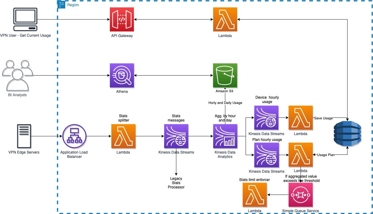
The solution has the following workflow:
- Usage data is collected by a VPN edge server and sends it to the backend service through Application Load Balancer.
- A single usage data record sent by the VPN edge server contains usage data for many users. A stats splitter splits the message into individual usage stats per user and forwards the message to Kinesis Data Streams.
- Usage data is consumed by both the legacy stats processor and the new Apache Flink application developed and deployed on Kinesis Data Analytics.
- The Apache Flink application carries out the following tasks:
- Aggregate device usage data hourly and send the aggregated result to Amazon S3 and the outgoing Kinesis data stream, which is picked up by a Lambda function that persists the usage data in DynamoDB.
- Aggregate device usage data daily and send the aggregated result to Amazon S3.
- Aggregate account usage data hourly and forward the aggregated results to the outgoing data stream, which is picked up by a Lambda function that checks if account usage is over the limit for that account. If account usage is over the limit, the function forwards the account information to another Lambda function, via Amazon Simple Queue Service (Amazon SQS), to cut off access on that account.
Design journey
NortonLifeLock needed a solution that was capable of real-time streaming and batch analytics. Kinesis Data Analysis fits this requirement because of the following key features:
- Real-time streaming and batch analytics for data aggregation
- Fully managed with a pay-as-you-go model
- Auto scaling
NortonLifeLock needed Kinesis Data Analytics to do the following:
- Aggregate customer usage data per device hourly and send results to Kinesis Data Streams (ultimately to DynamoDB) and the data lake (Amazon S3)
- Aggregate customer usage data per account hourly and send results to Kinesis Data Streams (ultimately to DynamoDB and Lambda, which enforces usage limit)
- Aggregate customer usage data per device daily and send results to the data lake (Amazon S3)
The legacy system processes usage data from an incoming Kinesis data stream, and they plan to use Kinesis Data Analytics to consume and process production data from the same stream. As such, NortonLifeLock started with SQL applications on Kinesis Data Analytics.
First attempt: Kinesis Data Analytics for SQL
Kinesis Data Analytics with SQL provides a high-level SQL-based abstraction for real-time stream processing and analytics. It’s configuration driven and very simple to get started. NortonLifeLock was able to create a prototype from scratch, get to production, and process the production load in less than 2 weeks. The solution met 90% of the requirements, and there were alternates for the remaining 10%.
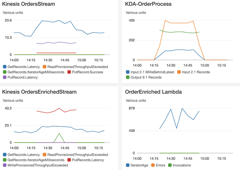
However, they started to receive “read limit exceeded” alerts from the source data stream, and the legacy application was read throttled. With Amazon Support’s help, they traced the issues to the drastic reversal of the Kinesis Data Analytics MillisBehindLatest metric in Kinesis record processing. This was correlated to the Kinesis Data Analytics auto scaling events and application restarts, as illustrated by the following diagram. The highlighted areas show the correlation between spikes due to autoscaling and reversal of MillisBehindLatest metrics.
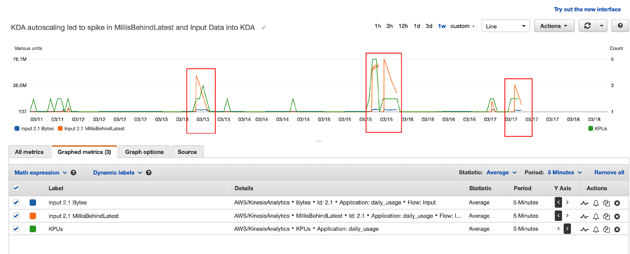
Here’s what happened:
- Kinesis Data Analytics for SQL scaled up KPU due to load automatically, and the Kinesis Data Analytics application was restarted (part of scaling up).
- Kinesis Data Analytics for SQL supports the at least once delivery model and uses checkpoints to ensure no data loss. But it doesn’t support taking a snapshot and restoring from the snapshot after a restart. For more details, see Delivery Model for Persisting Application Output to an External Destination.
- When the Kinesis Data Analytics for SQL application was restarted, it needed to reprocess data from the beginning of the aggregation window, resulting in a very large number of duplicate records, which led to a dramatic increase in the Kinesis Data Analytics
MillisBehindLatestmetric. - To catch up with incoming data, Kinesis Data Analytics started re-reading from the Kinesis data stream, which led to over-consumption of read throughput and the legacy application being throttled.
In summary, Kinesis Data Analytics for SQL’s duplicates record processing on restarts, no other means to eliminate duplicates, and limited ability to control auto scaling led to this issue.
Although they found Kinesis Data Analytics for SQL easy to get started, these limitations demanded other alternatives. NortonLifeLock reached out to the Kinesis Data Analytics team and discussed the following options:
- Option 1 – AWS was planning to release a new service, Kinesis Data Analytics Studio for SQL, Python, and Scala, which addresses these limitations. But this service was still a few months away (this service is now available, launched May 27, 2021).
- Option 2 – The alternative was to switch to Kinesis Data Analytics for Apache Flink, which also provides the necessary tools to address all their requirements.
Second attempt: Kinesis Data Analytics for Apache Flink
Apache Flink has a comparatively steep learning curve (we used Java for streaming analytics instead of SQL), and it took about 4 weeks to build the same prototype, deploy it to Kinesis Data Analytics, and test the application in production. NortonLifeLock had to overcome a few hurdles, which we document in this section along with the lessons learned.
Challenge 1: Too many writes to outgoing Kinesis data stream
The first thing they noticed was that the write threshold on the outgoing Kinesis data stream was greatly exceeded. Kinesis Data Analytics was attempting to write 10 times the amount of expected data to the data stream, with 95% of data throttled.
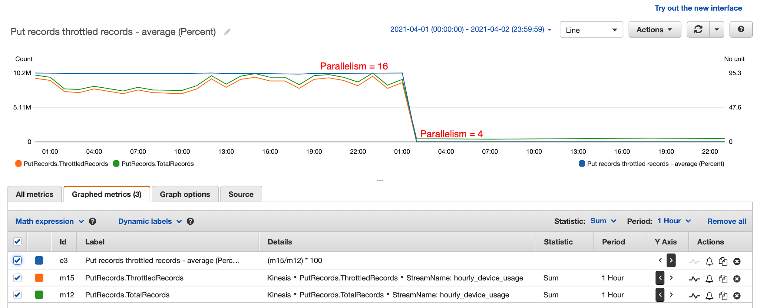
After a lengthy investigation, it turned out that having too much parallelism in the Kinesis Data Analytics application led to this issue. They had followed default recommendations and set parallelism to 12 and it scaled up to 16. This means that every hour, 16 separate threads were attempting to write to the destination data stream simultaneously, leading to massive contention and writes throttled. These threads attempted to retry continuously, until all records were written to the data stream. This resulted in 10 times the amount of data processing attempted, even though only one tenth of the writes eventually succeeded.
The solution was to reduce parallelism to 4 and disable auto scaling. In the preceding diagram, the percentage of throttled records dropped to 0 from 95% after they reduced parallelism to 4 in the Kinesis Data Analytics application. This also greatly improved KPU utilization and reduced Kinesis Data Analytics cost from $50 a day to $8 a day.
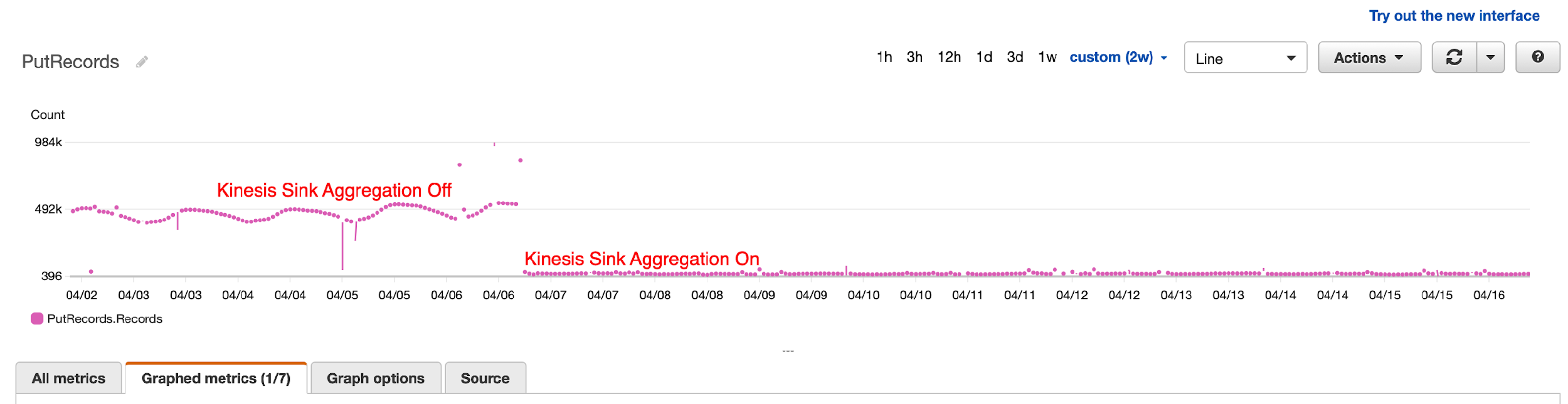
Challenge 2: Use Kinesis Data Analytics sink aggregation
After tuning parallelism, they still noticed occasional throttling by Kinesis Data Streams because of the number of records being written, not record size. To overcome this, they turned on Kinesis Data Analytics sink aggregation to reduce the number of records being written to the data stream, and the result was dramatic. They were able to reduce the number of writes by 1,000 times.
Challenge 3: Handle Kinesis Data Analytics Flink restarts and the resulting duplicate records
Kinesis Data Analytics applications restart because of auto scaling or recovery from application or task manager crashes. When this happens, Kinesis Data Analytics saves a snapshot before shutdown and automatically reloads the latest snapshot and picks up where the work was left off. Kinesis Data Analytics also saves a checkpoint every minute so no data is lost, guaranteeing exactly-once processing.
However, when the Kinesis Data Analytics application shut down in the middle of sending results to Kinesis Data Streams, it doesn’t guarantee exactly-once data delivery. In fact, Flink only guarantees at least once delivery to Kinesis Data Analytics sink, meaning that Kinesis Data Analytics guarantees to send a record at least once, which leads to duplicate records sent when Kinesis Data Analytics is restarted.
How were duplicate records handled in the outgoing data stream?
Because duplicate records aren’t handled by Kinesis Data Analytics when sinks do not have exactly-once semantics, the downstream application must deal with the duplicate records. The first question you should ask is whether it’s necessary to deal with the duplicate records. Maybe it’s acceptable to tolerate duplicate records in your application? This, however, is not an option for NortonLifeLock, because no user wants to have their available usage taken twice within the same hour. So, logic had to be built in the application to handle duplicate usage records.
To deal with duplicate records, you can employ a strategy in which the application saves an update timestamp along with the user’s latest usage. When a record comes in, the application reads existing daily usage and compares the update timestamp against the current time. If the difference is less than a configured window (50 minutes if the aggregation window is 60 minutes), the application ignores the new record because it’s a duplicate. It’s acceptable for the application to potentially undercount vs. overcount user usage.
How were duplicate records handled in the outgoing S3 bucket?
Kinesis Data Analytics writes temporary files in Amazon S3 before finalizing and removing them. When Kinesis Data Analytics restarts, it attempts to write new S3 files, and potentially leaves behind temporary S3 files because of restart. Because Athena ignores all temporary S3 files, no further is action needed. If your BI tools take temporary S3 files into consideration, you have to configure the Amazon S3 lifecycle policy to clean up temporary S3 files after a certain time.
Conclusion
NortonLifelock has been successfully running a Kinesis Data Analytics application in production since May 2021. It provides several key benefits. VPN users can now keep track of their usage in near-real time. BI analysts can get timely insights that are used for targeted sales and marketing campaigns, and upselling features and services. VPN usage limits are enforced in near-real time, thereby optimizing the network resources. NortonLifelock is saving tens of thousands of dollars each month with this real-time streaming analytics solution. And this telemetry solution is able to keep up with petabytes of data flowing through their global VPN service, which is seeing double-digit monthly growth.
To learn more about Kinesis Data Analytics and getting started with serverless streaming solutions on AWS, please see Developer Guide for Studio, the easiest way to build Apache Flink applications in SQL, Python, Scala in a notebook interface.
About the Authors
 Lei Gu has 25 years of software development experience and the architect for three key Norton products, Norton Secure Backup, VPN and Norton Family. He is passionate about cloud transformation and most recently spoke about moving from Cassandra to Amazon DynamoDB at AWS re:Invent 2019. Check out his Linkedin profile at https://www.linkedin.com/in/leigu/.
 Madhu Nunna is a Sr. Solutions Architect at AWS, with over 20 years of experience in networks and cloud, with the last two years focused on AWS Cloud. He is passionate about Analytics and AI/ML. Outside of work, he enjoys hiking and reading books on philosophy, economics, history, astronomy and biology.


 Jeremy Ber has been working in the telemetry data space for the past 5 years as a Software Engineer, Machine Learning Engineer, and most recently a Data Engineer. In the past, Jeremy has supported and built systems that stream in terabytes of data per day, and process complex machine learning algorithms in real time. At AWS, he is a Solutions Architect Streaming Specialist supporting both Managed Streaming for Kafka (Amazon MSK) and Amazon Kinesis.


 Wolfram “Wolle” Wingerath heads the data engineering team that is responsible for developing and operating Baqend’s infrastructure for analytics and reporting.
 Florian Bücklers is Baqend’s Chief Technology Officer and therefore responsible for coordinating between the different teams for front-end and backend development, devOps, onboarding, and data engineering.
 Benjamin Wollmer develops data-intensive systems at Baqend, but he is also doing his PhD at the University of Hamburg and therefore likes to read and write about related topics.
 Jörn Domnik is a Senior Software Engineer at Baqend with a focus on backend development and reliability engineering.
 As a DevOps engineer, Virginia Amberg monitors cluster health and keeps all systems running smoothly at Baqend.
 As a Principal Prototyping Engagement Manager in AWS, Markus Bestehorn is responsible for building business-critical prototypes with AWS customers and is a specialist for IoT and machine learning.
 As a Data Prototyping Architect in AWS, Anil Sener builds prototypes on big data analytics, data streaming, and machine learning, which accelerates the production journey on the AWS Cloud for top EMEA customers.
 As B2B Strategic Account Manager for Startups at AWS, Daniel Zäeh works with customers to make their ideas come true and helps them grow, by connecting tech and business.
 Brian Likosar is a Senior Streaming Specialist Solutions Architect at Amazon Web Services. Brian loves helping customers capture value from real-time streaming architectures, because he knows life doesn’t happen in batch. He’s a big fan of open-source collaboration, theme parks, and live music.
 Larry Heathcote is a Senior Product Marketing Manager at Amazon Web Services for data streaming and analytics. Larry is passionate about seeing the results of data-driven insights on business outcomes. He enjoys walking his Samoyed Sasha in the mornings so she can look for squirrels to bark at.
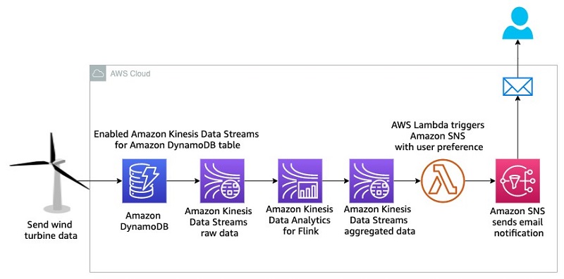


 Saurabh Shrivastava is a solutions architect leader and analytics/machine learning specialist working with global systems integrators. He works with AWS partners and customers to provide them with architectural guidance for building scalable architecture in hybrid and AWS environments. He enjoys spending time with his family outdoors and traveling to new destinations to discover new cultures.
 Sameer Goel is a solutions architect in Seattle who drives customers’ success by building prototypes on cutting-edge initiatives. Prior to joining AWS, Sameer graduated with a Master’s degree with a Data Science concentration from NEU Boston. He enjoys building and experimenting with creative projects and applications.
 Pratik Patel is a senior technical account manager and streaming analytics specialist. He works with AWS customers and provides ongoing support and technical guidance to help plan and build solutions by using best practices, and proactively helps keep customers’ AWS environments operationally healthy.


 Ram Vittal is an enterprise solutions architect at AWS. His current focus is to help enterprise customers with their cloud adoption and optimization journey to improve their business outcomes. In his spare time, he enjoys tennis, photography, and movies.
 Akash Bhatia is a Sr. solutions architect at AWS. His current focus is helping customers achieve their business outcomes through architecting and implementing innovative and resilient solutions at scale.

 Karthi Thyagarajan is a Principal Solutions Architect on the Amazon Kinesis team.
 Deepthi Mohan is a Sr. TPM on the Amazon Kinesis Data Analytics team.