Tag Archives: launch

AWS Network Firewall – New Managed Firewall Service in VPC

Post Syndicated from Channy Yun original https://aws.amazon.com/blogs/aws/aws-network-firewall-new-managed-firewall-service-in-vpc/

Our customers want to have a high availability, scalable firewall service to protect their virtual networks in the cloud. Security is the number one priority of AWS, which has provided various firewall capabilities on AWS that address specific security needs, like Security Groups to protect Amazon Elastic Compute Cloud (EC2) instances, Network ACLs to protect Amazon Virtual Private Cloud (VPC) subnets, AWS Web Application Firewall (WAF) to protect web applications running on Amazon CloudFront, Application Load Balancer (ALB) or Amazon API Gateway, and AWS Shield to protect against Distributed Denial of Service (DDoS) attacks.

We heard customers want an easier way to scale network security across all the resources in their workload, regardless of which AWS services they used. They also want customized protections to secure their unique workloads, or to comply with government mandates or commercial regulations. These customers need the ability to do things like URL filtering on outbound flows, pattern matching on packet data beyond IP/Port/Protocol and the ability to alert on specific vulnerabilities for protocols beyond HTTP/S.

Today, I am happy to announce AWS Network Firewall, a high availability, managed network firewall service for your virtual private cloud (VPC). It enables you to easily deploy and manage stateful inspection, intrusion prevention and detection, and web filtering to protect your virtual networks on AWS. Network Firewall automatically scales with your traffic, ensuring high availability with no additional customer investment in security infrastructure.

With AWS Network Firewall, you can implement customized rules to prevent your VPCs from accessing unauthorized domains, to block thousands of known-bad IP addresses, or identify malicious activity using signature-based detection. AWS Network Firewall makes firewall activity visible in real-time via CloudWatch metrics and offers increased visibility of network traffic by sending logs to S3, CloudWatch and Kinesis Firehose. Network Firewall is integrated with AWS Firewall Manager, giving customers who use AWS Organizations a single place to enable and monitor firewall activity across all your VPCs and AWS accounts. Network Firewall is interoperable with your existing security ecosystem, including AWS partners such as CrowdStrike, Palo Alto Networks, and Splunk. You can also import existing rules from community maintained Suricata rulesets.

Concepts of Network Firewall
AWS Network Firewall runs stateless and stateful traffic inspection rules engines. The engines use rules and other settings that you configure inside a firewall policy.

You use a firewall on a per-Availability Zone basis in your VPC. For each Availability Zone, you choose a subnet to host the firewall endpoint that filters your traffic. The firewall endpoint in an Availability Zone can protect all of the subnets inside the zone except for the one where it’s located.

You can manage AWS Network Firewall with the following central components.

  • Firewall – A firewall connects the VPC that you want to protect to the protection behavior that’s defined in a firewall policy. For each Availability Zone where you want protection, you provide Network Firewall with a public subnet that’s dedicated to the firewall endpoint. To use the firewall, you update the VPC route tables to send incoming and outgoing traffic through the firewall endpoints.
  • Firewall policy – A firewall policy defines the behavior of the firewall in a collection of stateless and stateful rule groups and other settings. You can associate each firewall with only one firewall policy, but you can use a firewall policy for more than one firewall.
  • Rule group – A rule group is a collection of stateless or stateful rules that define how to inspect and handle network traffic. Rules configuration includes 5-tuple and domain name filtering. You can also provide stateful rules using Suricata open source rule specification.

AWS Network Firewall – Getting Started
You can start AWS Network Firewall in AWS Management Console, AWS Command Line Interface (CLI), and AWS SDKs for creating and managing firewalls. In the navigation pane in VPC console, expand AWS Network Firewall and then choose Create firewall in Firewalls menu.

To create a new firewall, enter the name that you want to use to identify this firewall and select your VPC from the dropdown. For each availability zone (AZ) where you want to use AWS Network Firewall, create a public subnet to for the firewall endpoint. This subnet must have at least one IP address available and a non-zero capacity. Keep these firewall subnets reserved for use by Network Firewall.

For Associated firewall policy, select Create and associate an empty firewall policy and choose Create firewall.

Your new firewall is listed in the Firewalls page. The firewall has an empty firewall policy. In the next step, you’ll specify the firewall behavior in the policy. Select your newly created the firewall policy in Firewall policies menu.

You can create or add new stateless or stateful rule groups – zero or more collections of firewall rules, with priority settings that define their processing order within the policy, and stateless default action defines how Network Firewall handles a packet that doesn’t match any of the stateless rule groups.

For stateless default action, the firewall policy allows you to specify different default settings for full packets and for packet fragments. The action options are the same as for the stateless rules that you use in the firewall policy’s stateless rule groups.

You are required to specify one of the following options:

  • Allow – Discontinue all inspection of the packet and permit it to go to its intended destination.
  • Drop – Discontinue all inspection of the packet and block it from going to its intended destination.
  • Forward to stateful rule groups – Discontinue stateless inspection of the packet and forward it to the stateful rule engine for inspection.

Additionally, you can optionally specify a named custom action to apply. For this action, Network Firewall sends an CloudWatch metric dimension named CustomAction with a value specified by you. After you define a named custom action, you can use it by name in the same context where you have define it. You can reuse a custom action setting among the rules in a rule group and you can reuse a custom action setting between the two default stateless custom action settings for a firewall policy.

After you’ve defined your firewall policy, you can insert the firewall into your VPC traffic flow by updating the VPC route tables to include the firewall.

How to set up Rule Groups
You can create new stateless or stateful rule groups in Network Firewall rule groups menu, and choose Create rule group. If you select Stateful rule group, you can select one of three options: 1) 5-tuple format, specifying source IP, source port, destination IP, destination port, and protocol, and specify the action to take for matching traffic, 2) Domain list, specifying a list of domain names and the action to take for traffic that tries to access one of the domains, and 3) Suricata compatible IPS rules, providing advanced firewall rules using Suricata rule syntax.

Network Firewall supports the standard stateless “5 tuple” rule specification for network traffic inspection with priority number that indicates the processing order of the stateless rule within the rule group.

Similarly, a stateful 5 tuple rule has the following match settings. These specify what the Network Firewall stateful rules engine looks for in a packet. A packet must satisfy all match settings to be a match.

A rule group with domain names has the following match settings – Domain name, a list of strings specifying the domain names that you want to match, and Traffic direction, a direction of traffic flow to inspect. The following JSON shows an example rule definition for a domain name rule group.

{
  "RulesSource": {
    "RulesSourceList": {
      "TargetType": "FQDN_SNI","HTTP_HOST",
      "Targets": [
        "test.example.com",
        "test2.example.com"
      ],
      "GeneratedRulesType": "DENYLIST"
    }
  } 
}

A stateful rule group with Suricata compatible IPS rules has all settings defined within the Suricata compatible specification. For example, as following is to detect SSH protocol anomalies. For information about Suricata, see the Suricata website.

alert tcp any any -> any 22 (msg:"ALERT TCP port 22 but not SSH"; app-layer-protocol:!ssh; sid:2271009; rev:1;)

You can monitor Network Firewall using CloudWatch, which collects raw data and processes it into readable, near real-time metrics, and AWS CloudTrail, a service that provides a record of API calls to AWS Network Firewall by a user, role, or an AWS service. CloudTrail captures all API calls for Network Firewall as events. To learn more about logging and monitoring, see the documentation.

Network Firewall Partners
At this launch, Network Firewall integrates with a collection of AWS partners. They provided us with lots of helpful feedback. Here are some of the blog posts that they wrote in order to share their experiences (I am updating this article with links as they are published).

Available Now
AWS Network Firewall is now available in US East (N. Virginia), US West (Oregon), and Europe (Ireland) Regions. Take a look at the product page, price, and the documentation to learn more. Give this a try, and please send us feedback either through your usual AWS Support contacts or the AWS forum for Amazon VPC.

Learn all the details about AWS Network Firewall and get started with the new feature today.

— Channy;

Lightsail Containers: An Easy Way to Run your Containers in the Cloud

Post Syndicated from Sébastien Stormacq original https://aws.amazon.com/blogs/aws/lightsail-containers-an-easy-way-to-run-your-containers-in-the-cloud/

When I am delivering an introduction to the AWS Cloud for developers, I usually spend a bit of time to mention and to demonstrate Amazon Lightsail. It is by far the easiest way to get started on AWS. It allows you to get your application running on your own virtual server in a matter of minutes. Today, we are adding the possibility to deploy your container-based workloads on Amazon Lightsail. You can now deploy your container images to the cloud with the same simplicity and the same bundled pricing Amazon Lightsail provides for your virtual servers.

Amazon Lightsail is an easy-to-use cloud service that offers you everything needed to deploy an application or website, for a cost effective and easy to understand monthly plan. It is ideal to deploy simple workloads, websites, or to get started with AWS. The typical Lightsail customers range from developers to small businesses or startups who are looking to get quickly started in the cloud and AWS. At any time, you can later adopt the broad AWS Services when you are getting more familiar with the AWS cloud.

Under the hood, Lightsail is powered by Amazon Elastic Compute Cloud (EC2), Amazon Relational Database Service (RDS), Application Load Balancer, and other AWS services. It offers the level of security, reliability, and scalability you are expecting from AWS.

When deploying to Lightsail, you can choose between six operating systems (4 Linux distributions, FreeBSD, or Windows), seven applications (such as WordPress, Drupal, Joomla, Plesk…), and seven stacks (such as Node.js, Lamp, GitLab, Django…). But what about Docker containers?

Starting today, Amazon Lightsail offers an simple way for developers to deploy their containers to the cloud. All you need to provide is a Docker image for your containers and we automatically containerize it for you. Amazon Lightsail gives you an HTTPS endpoint that is ready to serve your application running in the cloud container. It automatically sets up a load balanced TLS endpoint, and take care of the TLS certificate. It replaces unresponsive containers for you automatically, it assigns a DNS name to your endpoint, it maintains the old version till the new version is healthy and ready to go live, and more.

Let’s see how it works by deploying a simple Python web app as a container. I assume you have the AWS Command Line Interface (CLI) and Docker installed on your laptop. Python is not required, it will be installed in the container only.

I first create a Python REST API, using the Flask simple application framework. Any programming language and any framework that can run inside a container works too. I just choose Python and Flask because they are simple and elegant.

You can safely copy /paste the following commands:

mkdir helloworld-python
cd helloworld-python
# create a simple Flask application in helloworld.py
echo "

from flask import Flask, request
from flask_restful import Resource, Api

app = Flask(__name__)
api = Api(app)

class Greeting (Resource):
   def get(self):
      return { "message" : "Hello Flask API World!" }
api.add_resource(Greeting, '/') # Route_1

if __name__ == '__main__':
   app.run('0.0.0.0','8080')

"  > helloworld.py

Then I create a Dockerfile that contains the steps and information required to build the container image:

# create a Dockerfile
echo '
FROM python:3
ADD helloworld.py /
RUN pip install flask
RUN pip install flask_restful
EXPOSE 8080
CMD [ "python", "./helloworld.py"]
 '  > Dockerfile

Now I can build my container:

docker build -t lightsail-hello-world .

The build command outputs many lines while it builds the container, it eventually terminates with the following message (actual ID differs):

Successfully built 7848e055edff
Successfully tagged lightsail-hello-world:latest

I test the container by launching it on my laptop:

docker run -it --rm -p 8080:8080 lightsail-hello-world

and connect a browser to localhost:8080

Testing Flask API in the container

When I am satisfied with my app, I push the container to Docker Hub.

docker tag lightsail-hello-world sebsto/lightsail-hello-world
docker login
docker push sebsto/lightsail-hello-world

Now that I have a container ready on Docker Hub, let’s create a Lightsail Container Service.

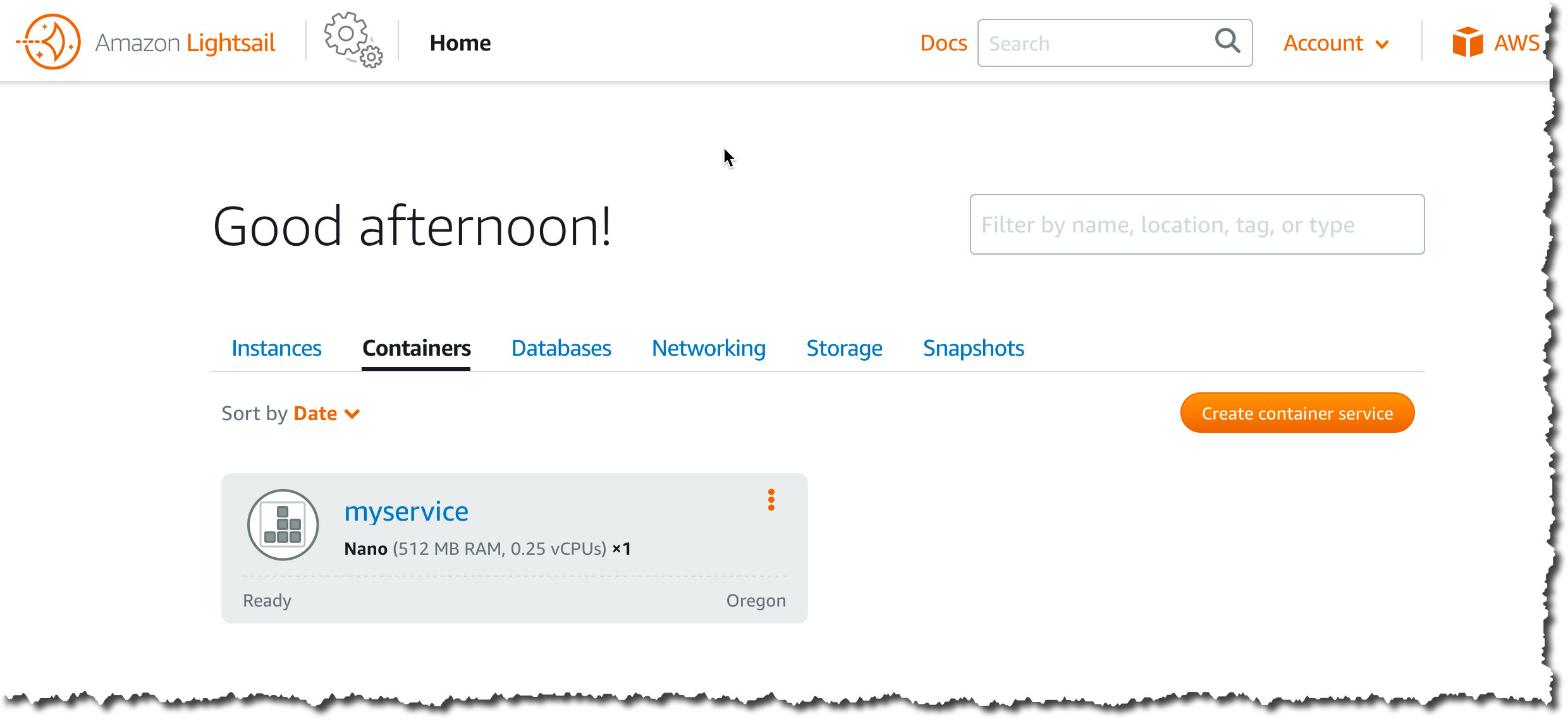
I point my browser to the Amazon Lightsail console. I can see container services already deployed and I can manage them. To create a new service, I click Create container service:Lighsail Container Console

On the next screen, I select the size of the container I want to use, in terms of vCPU and memory available to my application. I also select the number of container instances I want to run in parallel for high availability or scalability reasons. I can change the number of container instances or their power (vCPU and RAM) at any time, without interrupting the service. Both these parameters impact the price AWS charges you per month. The price is indicated and dynamically adjusted on the screen, as shown on the following video.

Lightsail choose capacity

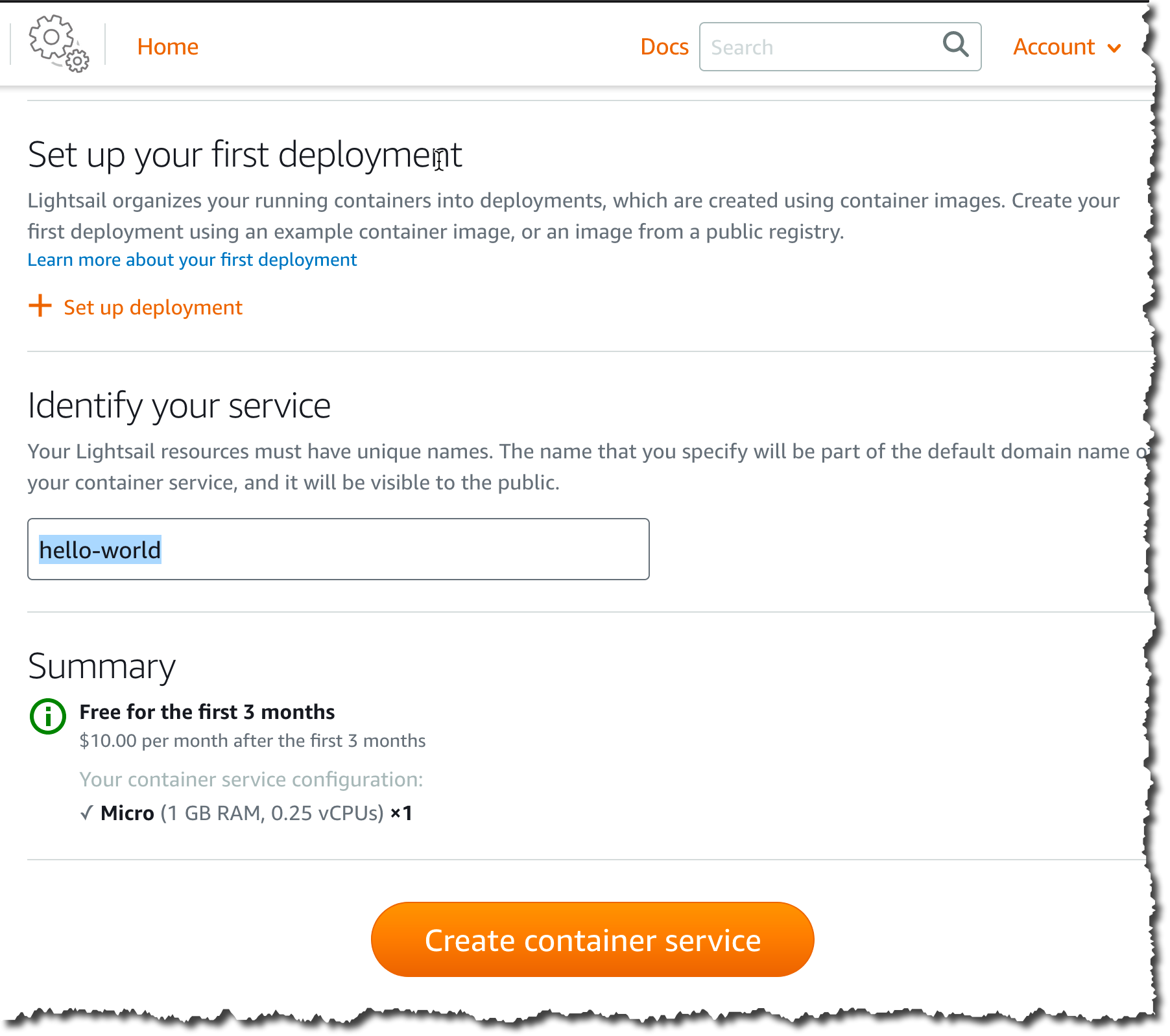
Slightly lower on the screen, I choose to skip the deployment for now. I give a name for the service (“hello-world“). I click Create container service.

Lightsail container name

Once the service is created, I click Create your first deployment to create a deployment. A deployment is a combination of a specific container image and version to be deployed on the service I just created.

I chose a name for my image and give the address of the image on Docker Hub, using the format user/<my container name>:tag. This is also where I have the possibility to enter environment variables, port mapping, or a launch command.

My container is offering a network service on port TCP 8080, so I add that port to the deployment configuration. The Open Ports configuration specifies which ports and protocols are open to other systems in my container’s network. Other containers or virtual machines can only connect to my container when the port is explicitly configured in the console or EXPOSE‘d in my Dockerfile. None of these ports are exposed to the public internet.

But in this example, I also want Lightsail to route the traffic from the public internet to this container. So, I add this container as an endpoint of the hello-world service I just created. The endpoint is automatically configured for TLS, there is no certificate to install or manage.

I can add up to 10 containers for one single deployment. When ready, I click Save and deploy.

Lightsail Deployment

After a while, my deployment is active and I can test the endpoint.

Lightsail Deployment Active

The endpoint DNS address is available on the top-right side of the console. If I must, I can configure my own DNS domain name.

Lightsail endpoint DNSI open another tab in my browser and point it at the https endpoint URL:

Testing Container DeploymentWhen I must deploy a new version, I use the console again to modify the deployment. I spare you the details of modifying the application code, build, and push a new version of the container. Let’s say I have my second container image version available under the name sebsto/lightsail-hello-world:v2. Back to Amazon Lightsail console, I click Deployments, then Modify your Deployments. I enter the full name, including the tag, of the new version of the container image and click Save and Deploy.

Lightsail Deploy updated VersionAfter a while, the new version is deployed and automatically activated.

Lightsail deployment sucesful

I open a new tab in my browser and I point it to the endpoint URI available on the top-right corner of Amazon Lightsail console. I observe the JSON version is different. It now has a version attribute with a value of 2.

lightsail v2 is deployed

When something goes wrong during my deployment, Amazon Lightsail automatically keeps the last deployment active, to avoid any service interruption. I can also manually activate a previous deployment version to reverse any undesired changes.

I just deployed my first container image from Docker Hub. I can also manage my services and deploy local container images from my laptop using the AWS Command Line Interface (CLI). To push container images to my Amazon Lightsail container service directly from my laptop, I must install the LightSail Controler Plugin. (TL;DR curl, cp and chmod are your friends here, I also maintain a DockerFile to use the CLI inside a container.)

To create, list, or delete a container service, I type:

aws lightsail create-container-service --service-name myservice --power nano --scale 1

aws lightsail get-container-services
{
   "containerServices": [{
      "containerServiceName": "myservice",
      "arn": "arn:aws:lightsail:us-west-2:012345678901:ContainerService/1b50c121-eac7-4ee2-9078-425b0665b3d7",
      "createdAt": "2020-07-31T09:36:48.226999998Z",
      "location": {
         "availabilityZone": "all",
         "regionName": "us-west-2"
      },
      "resourceType": "ContainerService",
      "power": "nano",
      "powerId": "",
      "state": "READY",
      "scale": 1,
      "privateDomainName": "",
      "isDisabled": false,
      "roleArn": ""
   }]
}

aws lightsail delete-container-service --service myservice

I can also use the CLI to deploy container images directly from my laptop. Be sure lightsailctl is installed.

# Build the new version of my image (v3)
docker build -t sebsto/lightsail-hello-world:v3 .

# Push the new image.
aws lightsail push-container-image --service-name hello-world --label hello-world --image sebsto/lightsail-hello-world:v3

After a while, I see the output:

Image "sebsto/lightsail-hello-world:v3" registered.
Refer to this image as ":hello-world.hello-world.1" in deployments.

I create a lc.json file to hold the details of the deployment configuration. it is aligned to the options I see on the console. I report the name given by the previous command on the image property:

{
  "serviceName": "hello-world",
  "containers": {
     "hello-world": {
        "image": ":hello-world.hello-world.1",
        "ports": {
           "8080": "HTTP"
        }
     }
  },
  "publicEndpoint": {
     "containerName": "hello-world",
     "containerPort": 8080
  }
}

Finally, I create a new service version with:
aws lightsail create-container-service-deployment --cli-input-json file://lc.json

I can query the deployment status with
aws lightsail get-container-services

...
"nextDeployment": {
   "version": 4,
   "state": "ACTIVATING",
   "containers": {
      "hello-world": {
      "image": ":hello-world.hello-world.1",
      "command": [],
      "environment": {},
      "ports": {
         "8080": "HTTP"
      }
     }
},
...

After a while, the status  becomes  ACTIVE, and I can test my endpoint.

curl https://hello-world.nxxxxxxxxxxx.lightsail.ec2.aws.dev/
{"message": "Hello Flask API World!", "version": 3}

If you plan to later deploy your container to Amazon ECS or Amazon Elastic Kubernetes Service, no changes are required. You can pull the container image from your repository, just like you do with Amazon Lightsail.

You can deploy your containers on Lightsail in all AWS Regions where Amazon Lightsail is available. As of today, this is US East (Ohio), US East (N. Virginia), US West (Oregon), Asia Pacific (Mumbai), Asia Pacific (Seoul), Asia Pacific (Singapore), Asia Pacific (Sydney), Asia Pacific (Tokyo), Canada (Central), Europe (Frankfurt), Europe (Ireland), Europe (London), and Europe (Paris).

As usual when using Amazon Lightsail, pricing is easy to understand and predictable. Amazon Lightsail Containers have a fixed price per month per container, depending on the size of the container (the vCPU/memory combination you use). You are charged on the prorated hours you keep the service running. The price per month is the maximum price you will be charged for running your service 24h/7. The prices are identical in all AWS Regions. They are ranging from $7 / month for a Nano container (512MB memory and 0.25 vCPU) to $160 / month for a X-Large container (8GB memory and 4 vCPU cores). This price not only includes the container itself, but also the load balancer, the DNS, and a generous data transfer tier. The details and prices for other AWS Regions are on the Lightsail pricing page.

I can’t wait to discover what solutions you will build and deploy on Amazon Lightsail Containers!

— seb

Meet the newest AWS Heroes including the first DevTools Heroes!

Post Syndicated from Ross Barich original https://aws.amazon.com/blogs/aws/meet-the-newest-aws-heroes-including-the-first-devtools-heroes/

The AWS Heroes program recognizes individuals from around the world who have extensive AWS knowledge and go above and beyond to share their expertise with others. The program continues to grow, to better recognize the most influential community leaders across a variety of technical disciplines.

Introducing AWS DevTools Heroes
Today we are introducing AWS DevTools Heroes: passionate advocates of the developer experience on AWS and the tools that enable that experience. DevTools Heroes excel at sharing their knowledge and building community through open source contributions, blogging, speaking, community organizing, and social media. Through their feedback, content, and contributions DevTools Heroes help shape the AWS developer experience and evolve the AWS DevTools, such as the AWS Cloud Development Kit, the AWS SDKs, and AWS Code suite of services.

The first cohort of AWS DevTools Heroes include:

Bhuvaneswari Subramani – Bengaluru, India

DevTools Hero Bhuvaneswari Subramani is Director Engineering Operations at Infor. With two decades of IT experience, specializing in Cloud Computing, DevOps, and Performance Testing, she is one of the community leaders of AWS User Group Bengaluru. She is also an active speaker at AWS community events and industry conferences, and delivers guest lectures on Cloud Computing for staff and students at engineering colleges across India. Her workshops, presentations, and blogs on AWS Developer Tools always stand out.

Jared Short – Washington DC, USA

DevTools Hero Jared Short is an engineer at Stedi, where they are using AWS native tooling and serverless services to build a global network for exchanging B2B transactions in a standard format. Jared’s work includes early contributions to the Serverless Framework. These days, his focus is working with AWS CDK and other toolsets to create intuitive and joyful developer experiences for teams on AWS.

Matt Coulter – Belfast, Northern Ireland

DevTools Hero Matt Coulter is a Technical Architect for Liberty IT, focused on creating the right environment for empowered teams to rapidly deliver business value in a well-architected, sustainable, and serverless-first way. Matt has been creating this environment by building CDK Patterns, an open source collection of serverless architecture patterns built using AWS CDK that reference the AWS Well Architected Framework. Matt also created CDK Day, which was the first community driven, global conference focused on everything CDK (AWS CDK, CDK for Terraform, CDK for Kubernetes, and others).

Paul Duvall – Washington DC, USA

DevTools Hero Paul Duvall is co-founder and former CTO of Stelligent. He is principal author of “Continuous Integration: Improving Software Quality and Reducing Risk,” and is also the author of many other publications including “Continuous Compliance on AWS,” “Continuous Encryption on AWS,” and “Continuous Security on AWS.” Paul hosted the DevOps on AWS Radio podcast for over three years and has been an enthusiastic user and advocate of AWS Developer Tools since their respective releases.

Sebastian Korfmann – Hamburg, Germany

DevTools Hero Sebastian Korfmann is an entrepreneurial Software Engineer with a current focus on Cloud Tooling, Infrastructure as Code, and the Cloud Development Kit (CDK) ecosystem in particular. He is a core contributor to the CDK for Terraform project, which enables users to define infrastructure using TypeScript, Python, and Java while leveraging the hundreds of providers and thousands of module definitions provided by Terraform and the Terraform ecosystem. With cdk.dev, Sebastian co-founded a community-driven hub for all things CDK, and he runs a weekly newsletter covering the growing CDK ecosystem.

Steve Gordon – East Sussex, United Kingdom

DevTools Hero Steve Gordon is a Pluralsight author and senior engineer who is passionate about community and all things .NET related, having worked with .NET for over 16 years. Steve has used AWS extensively for five years as a platform for running .NET microservices. He blogs regularly about running .NET on AWS, including deep dives into how the .NET SDK works, building cloud-native services, and how to deploy .NET containers to Amazon ECS. Steve founded .NET South East, a .NET Meetup group based in Brighton.

Thorsten Höger – Stuttgart, Germany

DevTools Hero Thorsten Höger is CEO and cloud consultant at Taimos, where he is advising customers on how to use AWS. Being a developer, he focuses on improving development processes and automating everything to build efficient deployment pipelines for customers of all sizes. As a supporter of open-source software, Thorsten is maintaining or contributing to several projects on GitHub, like test frameworks for AWS Lambda, Amazon Alexa, or developer tools for AWS. He is also the maintainer of the Jenkins AWS Pipeline plugin and one of the top three non-AWS contributors to AWS CDK.


Meet the rest of the new AWS Heroes
There is more good news! We are thrilled to introduce the remaining new AWS Heroes in this cohort, including the first Heroes from Argentina, Lebanon, and Saudi Arabia:

Ahmed Samir – Riyadh, Saudi Arabia

Community Hero Ahmed Samir is a Cloud Architect and mentor with more than 12 years of experience in IT. He is the leader of three Arabic Meetups in Riyadh: AWS, Amazon SageMaker, and Kubernetes, where he has organized and delivered over 40 Meetup events. Ahmed frequently shares knowledge and evangelizes AWS in Arabic through his social media accounts. He also holds AWS and Kubernetes certifications.

Anas Khattar – Beirut, Lebanon

Community Hero Anas Khattar is co-founder of Digico Solutions. He founded the AWS User Group Lebanon in 2018 and coordinates monthly meetups and workshops on a variety of cloud topics, which helped grow the group to more than 1,000 AWSome members. He also regularly speaks at tech conferences and authors tech blogs on Dev Community, sharing his AWS experiences and best practices. In close collaboration with the regional AWS community leaders and builders, Anas organized AWS Community Day MENA, which started in September 2020 with 12 User Groups from 10 countries, and hosted 27 speakers over 2 days.

Chris Gong – New York, USA

Community Hero Chris Gong is constantly exploring the different ways that cloud services can be applied in game development. Passionate about sharing his knowledge with the world, he routinely creates tutorials and educational videos on his YouTube channel, Flopperam, where the primary focus has been AWS Game Tech and Unreal Engine, specifically the multiplayer and networking aspects of game development. Although Amazon GameLift has been his biggest interest, Chris has plans to cover the usage of other AWS services in game development while exploring how they can be integrated with other game engines besides Unreal Engine.

Damian Olguin – Cordoba, Argentina

Community Hero Damian Olguin is a tech entrepreneur and one of the founders of Teracloud, an AWS APN Partner. As a community leader, he promotes knowledge-sharing experiences in user communities within LATAM. He is co-organizer of AWS User Group Cordoba and co-host of #DeepFridays, a Twitch streaming show that promotes AI/ML technology adoption by playing with DeepRacer, DeepLens, and DeepComposer. Damian is a public speaker who has spoken at AWS Community Day Buenos Aires 2019, AWS re:Invent 2019, and AWS Community Day LATAM 2020.

Denis Bauer – Sydney, Australia

Data Hero Denis Bauer is a Principal Research Scientist at Australia’s government research agency (CSIRO). Her open source products include VariantSpark, the Machine Learning tool for analysing ultra-high dimensional data, which was the first AWS Marketplace health product from a public sector organization. Denis is passionate about facilitating the digital transformation of the health and life-science sector by building a strong community of practice through open source technology, keynote presentations, and inclusive interdisciplinary collaborations. For example, the collaboration with her organization’s visionary Scientific Computing and Cloud Platforms experts as well as AWS Data Hero Lynn Langit has enabled the creation of cloud-based bioinformatics solutions used by 10,000 researchers annually.

Denis Dyack – St. Catharines, Canada

Community Hero Denis Dyack, a video game industry veteran of more than 30 years, is the Founder and CEO of Apocalypse Studios. His studio evangelizes using a cloud-first approach in game development and partners with AWS Game Tech to move the medium of the games industry forward. In his years of experience speaking at games conferences and within AWS communities, Denis has been an advocate for building on Amazon Lumberyard and more recently in moving over game development pipelines to AWS.

Emrah Şamdan – Ankara, Turkey

Serverless Hero Emrah Şamdan is the VP of Products at Thundra. In order to expand the serverless community globally in a pandemic, he co-organized the quarterly held ServerlessDays Virtual. He’s also a local community organizer for AWS Community Day Turkey, ServerlessDays Istanbul, and bi-weekly meetups at Cloud and Serverless Turkey. He’s currently part of the core organizer team of global ServerlessDays and is continuously looking for ways to expand the community. He frequently writes about serverless and cloud-native microservices on Medium and on the Thundra blog.

Franck Pachot – Lausanne, Switzerland

Data Hero Franck Pachot is the Principal Consultant and Database Evangelist at dbi services (an AWS Select Partner) and is passionate about all databases. With over 20 years of experience in development, data modeling, infrastructure, and all DBA tasks, Franck is a recognized database expert across Oracle and AWS. Franck is also an AWS Academy educator for Powercoders, and holds AWS Certified Database Specialty and Oracle Certified Master certifications. Franck contributes to technical communities, educating customers on AWS Databases through his blog, Twitter, and podcast in French. He is active in the Data community, and enjoys talking and meeting other data enthusiasts at conferences.

Hiroko Nishimura – Washington DC, USA

Community Hero Hiroko Nishimura (Hiro) is the founder of AWS Newbies and Cloud Newbies, which help people with non-traditional technical backgrounds begin their explorations into the AWS Cloud. As a “career switcher” herself, she has been community building since 2018 to help others deconstruct Cloud Computing jargon so they, too, can begin a career in the Cloud. Finally putting her degrees in Special Education to good use, Hiro teaches “Introduction to AWS for Non-Engineers” courses at LinkedIn Learning, and introductory coding lessons at egghead.

Juliano Cristian – Santa Catarina, Brazil

Community Hero Juliano Cristian is CEO of Game Business Accelerator Academy and co-founder of Game Developers SC which participates in the AWS APN program. He organizes the AWS Game Tech Lumberyard User Group in Florianópolis, Brazil, holding Meetups, Practical Labs, Game Jams, and Workshops. He also conducts many lectures at universities, speaking with more than 90 educational institutions across Brazil, introducing students to cloud computing and AWS Game Tech services. Whenever he can, Juliano also participates in other AWS User Groups in Brazil and Latin America, working to build an increasingly motivated and productive community.

Jungyoul Yu – Seoul, Korea

Machine Learning Hero Jungyoul Yu works at Danggeun Market as a DevOps Engineer, and is a leader of the AWS DeepRacer Group, part of the AWS Korea User Group. He was one of the AWS DeepRacer League finalists in AWS Summit Seoul and AWS re:Invent 2019. Starting off with zero ML experience, Jungyoul used AWS DeepRacer to learn ML techniques and began sharing his learnings both in the AWS DeepRacer Community, with User Groups, at AWS Community Day, and at various meetups. He has also shared many blog posts and sample code such as DeepRacer Reward Function Simulator, Rank Notifier, and Auto submit bot.

Juv Chan – Singapore

Machine Learning Hero Juv Chan is an AI automation engineer at UBS. He is the AWS DeepRacer League Singapore Summit 2019 champion and a re:Invent Championship Cup 2019 finalist. He is the lead organizer for the AWS DeepRacer Beginner Challenge global virtual community race in 2020. Juv is also involved in sharing his DeepRacer and Machine Learning knowledge with the AWS Machine Learning community at both global and regional scale. Juv is a contributing writer for both Towards Data Science and Towards AI platforms, where he blogs about AWS AI/ML and cloud relevant topics.

Lukonde Mwila – Johannesburg, South Africa

Container Hero Lukonde Mwila is a Senior Software Engineer at Entelect. He has a passion for sharing knowledge through speaking engagements such as meetups and tech conferences, as well as writing technical articles. His talk at DockerCon 2020 on deploying multi-container applications to AWS was one of the top rated and most viewed sessions of the event. He is 3x AWS certified and is an advocate for containerization and serverless technologies. Lukonde enjoys sharing experiences of building out AWS infrastructure on Medium and sharing open source projects on GitHub for the developer community to easily consume, replicate, and improve for their own benefit.

Magdalena Zawada – Rybnik, Poland

Community Hero Magdalena Zawada is Director of Strategy and Expansion at LCloud Ltd. She has been working in IT for 11 years and started her adventure with AWS technology in 2013 as CEO of Hostersi Ltd. Magdalena willingly shares her knowledge and experience with the community, co-organizing AWS UG Warsaw meetings. She also organizes a series of events to support preparation for obtaining AWS Cloud Practitioner Certifications. Magdalena belongs to numerous industry organizations, including FinOps Foundation and ISSA Information Systems Security Association Poland, and in 2019 she was a participant of the AWS re:Invent Community Leader “We Power Tech” Diversity Grant in Las Vegas.

Nick Walter – Lincoln, USA

Data Hero Nick Walter has over 15 years of experience with enterprise IT solutions, including expertise and certifications in AWS, VMware, and Oracle. A passionate evangelist for data management solutions on AWS, Nick can often be found blogging, hosting webinars, or presenting at conferences regarding the latest trends in business critical database technologies. Recently, Nick has focused on helping clients find cost effective ways to handle both the technical and licensing challenges of migrating application stacks backed by commercial database engines, such as Oracle or MS SQL Server, into AWS.

Renato Losio – Berlin, Germany

Data Hero Renato Losio is the Principal Cloud Architect at Funambol, a provider of white label cloud services. He has been working with AWS technologies since 2011, and holds 7 AWS certifications (including the Database Specialty). Renato enjoys speaking at international events, including DevOps Pro Europe, DevOpsConf Russia, All Day DevOps, Codemotion, and Percona Live. Passionate about knowledge sharing, Renato is an editor at InfoQ and writes about different cloud-related topics on his blog, cloudiamo.com. Through his various platforms, he has covered different topics across AWS Databases, such as Amazon RDS Proxy, Amazon RDS, and Amazon Aurora.

Tomasz Lakomy – Poznan, Poland

Community Hero Tomasz Lakomy is a Senior Frontend Engineer at OLX Group, and an egghead.io instructor. Over the last two years, he’s been diving into the world of AWS and sharing what he’s learned with others. After passing the AWS Certified Solutions Architect: Associate exam in 2019 he has recorded multiple courses on serverless technologies, including “Build an App with the AWS Cloud Development Kit” and “Learn AWS Lambda from Scratch.” In addition, he’s active on his Twitter, blog (tlakomy.com), as well as The Practical Dev community, where he posts articles on career advice, testing and – of course – AWS.


If you’d like to learn more about the new Heroes, or connect with a Hero near you, please visit the AWS Hero website.

— Ross;

Announcing AWS Glue DataBrew – A Visual Data Preparation Tool That Helps You Clean and Normalize Data Faster

Post Syndicated from Danilo Poccia original https://aws.amazon.com/blogs/aws/announcing-aws-glue-databrew-a-visual-data-preparation-tool-that-helps-you-clean-and-normalize-data-faster/

To be able to run analytics, build reports, or apply machine learning, you need to be sure the data you’re using is clean and in the right format. That’s the data preparation step that requires data analysts and data scientists to write custom code and do many manual activities. First, you need to look at the data, understand which possible values are present, and build some simple visualizations to understand if there are correlations between the columns. Then, you need to check for strange values outside of what you’re expecting, such as weather temperature above 200℉ (93℃) or speed of a truck above 200 mph (322 km/h), or for data that is missing. Many algorithms need values to be rescaled to a specific range, for example between 0 and 1, or normalized around the mean. Text fields need to be set to a standard format, and may require advanced transformations such as stemming.

That’s a lot of work. For this reason, I am happy to announce that today AWS Glue DataBrew is available, a visual data preparation tool that helps you clean and normalize data up to 80% faster so you can focus more on the business value you can get.

DataBrew provides a visual interface that quickly connects to your data stored in Amazon Simple Storage Service (S3), Amazon Redshift, Amazon Relational Database Service (RDS), any JDBC accessible data store, or data indexed by the AWS Glue Data Catalog. You can then explore the data, look for patterns, and apply transformations. For example, you can apply joins and pivots, merge different data sets, or use functions to manipulate data.

Once your data is ready, you can immediately use it with AWS and third-party services to gain further insights, such as Amazon SageMaker for machine learning, Amazon Redshift and Amazon Athena for analytics, and Amazon QuickSight and Tableau for business intelligence.

How AWS Glue DataBrew Works
To prepare your data with DataBrew, you follow these steps:

  • Connect one or more datasets from S3 or the Glue data catalog (S3, Redshift, RDS). You can also upload a local file to S3 from the DataBrew console. CSV, JSON, Parquet, and .XLSX formats are supported.
  • Create a project to visually explore, understand, combine, clean, and normalize data in a dataset. You can merge or join multiple datasets. From the console, you can quickly spot anomalies in your data with value distributions, histograms, box plots, and other visualizations.
  • Generate a rich data profile for your dataset with over 40 statistics by running a job in the profile view.
  • When you select a column, you get recommendations on how to improve data quality.
  • You can clean and normalize data using more than 250 built-in transformations. For example, you can remove or replace null values, or create encodings. Each transformation is automatically added as a step to build a recipe.
  • You can then save, publish, and version recipes, and automate the data preparation tasks by applying recipes on all incoming data. To apply recipes to or generate profiles for large datasets, you can run jobs.
  • At any point in time, you can visually track and explore how datasets are linked to projects, recipes, and job runs. In this way, you can understand how data flows and what are the changes. This information is called data lineage and can help you find the root cause in case of errors in your output.

Let’s see how this works with a quick demo!

Preparing a Sample Dataset with AWS Glue DataBrew
In the DataBrew console, I select the Projects tab and then Create project. I name the new project Comments. A new recipe is also created and will be automatically updated with the data transformations that I will apply next.

I choose to work on a New dataset and name it Comments.

Here, I select Upload file and in the next dialog I upload a comments.csv file I prepared for this demo. In a production use case, here you will probably connect an existing source on S3 or in the Glue Data Catalog. For this demo, I specify the S3 destination for storing the uploaded file. I leave Encryption disabled.

The comments.csv file is very small, but will help show some common data preparation needs and how to complete them quickly with DataBrew. The format of the file is comma-separated values (CSV). The first line contains the name of the columns. Then, each line contains a text comment and a numerical rating made by a customer (customer_id) about an item (item_id). Each item is part of a category. For each text comment, there is an indication of the overall sentiment (comment_sentiment). Optionally, when giving the comment, customers can enable a flag to ask to be contacted for further support (support_needed).

Here’s the content of the comments.csv file:

customer_id,item_id,category,rating,comment,comment_sentiment,support_needed
234,2345,"Electronics;Computer", 5,"I love this!",Positive,False
321,5432,"Home;Furniture",1,"I can't make this work... Help, please!!!",negative,true
123,3245,"Electronics;Photography",3,"It works. But I'd like to do more",,True
543,2345,"Electronics;Computer",4,"Very nice, it's going well",Positive,False
786,4536,"Home;Kitchen",5,"I really love it!",positive,false
567,5432,"Home;Furniture",1,"I doesn't work :-(",negative,true
897,4536,"Home;Kitchen",3,"It seems OK...",,True
476,3245,"Electronics;Photography",4,"Let me say this is nice!",positive,false

In the Access permissions, I select a AWS Identity and Access Management (IAM) role which provides DataBrew read permissions to my input S3 bucket. Only roles where DataBrew is the service principal for the trust policy are shown in the DataBrew console. To create one in the IAM console, select DataBrew as trusted entity.

If the dataset is big, you can use Sampling to limit the number of rows to use in the project. These rows can be selected at the beginning, at the end, or randomly through the data. You are going to use projects to create recipes, and then jobs to apply recipes to all the data. Depending on your dataset, you may not need access to all the rows to define the data preparation recipe.

Optionally, you can use Tagging to manage, search, or filter resources you create with AWS Glue DataBrew.

The project is now being prepared and in a few minutes I can start exploring my dataset.

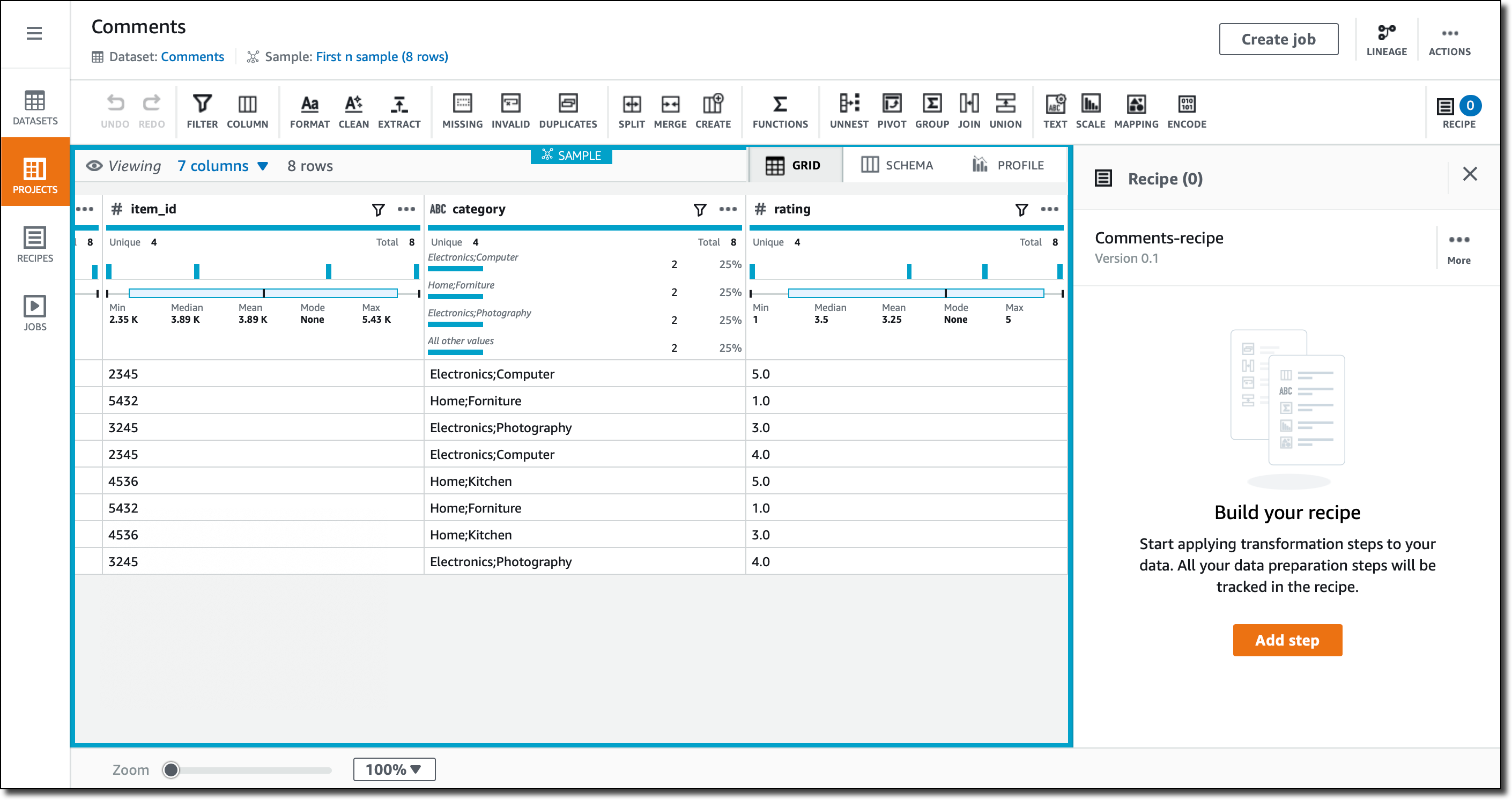
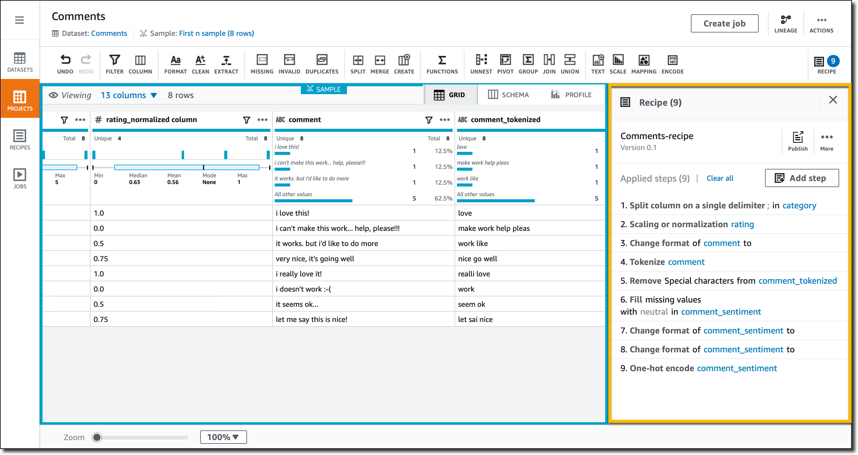
In the Grid view, the default when I create a new project, I see the data as it has been imported. For each column, there is a summary of the range of values that have been found. For numerical columns, the statistical distribution is given.

In the Schema view, I can drill down on the schema that has been inferred, and optionally hide some of the columns.

In the Profile view, I can run a data profile job to examine and collect statistical summaries about the data. This is an assessment in terms of structure, content, relationships, and derivation. For a large dataset, this is very useful to understand the data. For this small example the benefits are limited, but I run it nonetheless, sending the output of the profile job to a different folder in the same S3 bucket I use to store the source data.

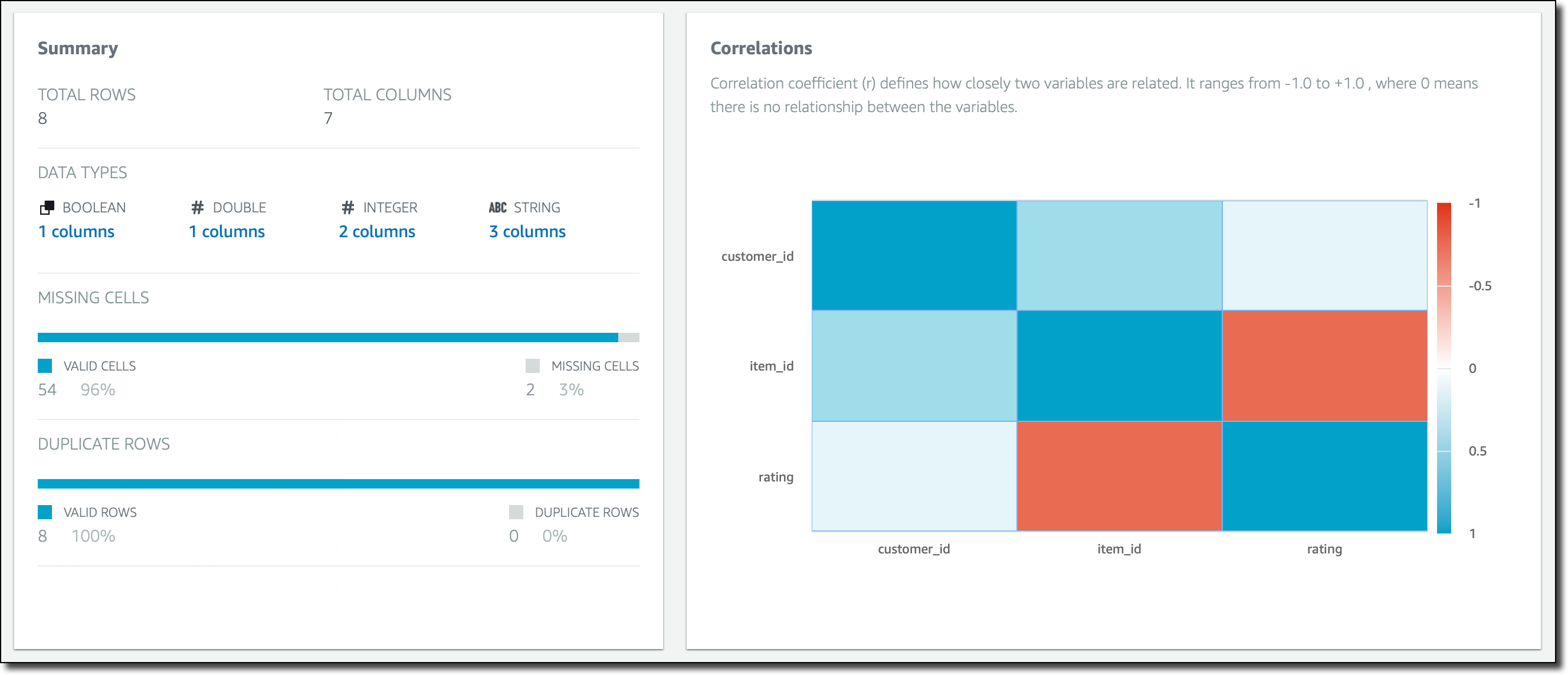
When the profile job has succeeded, I can see a summary of the rows and columns in my dataset, how many columns and rows are valid, and correlations between columns.

Here, if I select a column, for example rating, I can drill down into specific statistical information and correlations for that column.

Now, let’s do some actual data preparation. In the Grid view, I look at the columns. The category contains two pieces of information, separated by a semicolon. For example, the category of the first row is “Electronics;Computers.” I select the category column, then click on the column actions (the three small dots on the right of the column name) and there I have access to many transformations that I can apply to the column. In this case, I select to split the column on a single delimiter. Before applying the changes, I quickly preview them in the console.

I use the semicolon as delimiter, and now I have two columns, category_1 and category_2. I use the column actions again to rename them to category and subcategory. Now, for the first row, category contains Electronics and subcategory Computers. All these changes are added as steps to the project recipe, so that I’ll be able to apply them to similar data.

The rating column contains values between 1 and 5. For many algorithms, I prefer to have these kind of values normalized. In the column actions, I use min-max normalization to rescale the values between 0 and 1. More advanced techniques are available, such as mean or Z-score normalization. A new rating_normalized column is added.

I look into the recommendations that DataBrew gives for the comment column. Since it’s text, the suggestion is to use a standard case format, such as lowercase, capital case, or sentence case. I select lowercase.

The comments contain free text written by customers. To simplify further analytics, I use word tokenization on the column to remove stop words (such as “a,” “an,” “the”), expand contractions (so that “don’t” becomes “do not”), and apply stemming. The destination for these changes is a new column, comment_tokenized.

I still have some special characters in the comment_tokenized column, such as an emoticon :-). In the column actions, I select to clean and remove special characters.

I look into the recommendations for the comment_sentiment column. There are some missing values. I decide to fill the missing values with a neutral sentiment. Now, I still have values written with a different case, so I follow the recommendation to use lowercase for this column.

The comment_sentiment column now contains three different values (positive, negative, or neutral), but many algorithms prefer to have one-hot encoding, where there is a column for each of the possible values, and these columns contain 1, if that is the original value, or 0 otherwise. I select the Encode icon in the menu bar and then One-hot encode column. I leave the defaults and apply. Three new columns for the three possible values are added.

The support_needed column is recognized as boolean, and its values are automatically formatted to a standard format. I don’t have to do anything here.

The recipe for my dataset is now ready to be published and can be used in a recurring job processing similar data. I didn’t have a lot of data, but the recipe can be used with much larger datasets.

In the recipe, you can find a list of all the transformations that I just applied. When running a recipe job, output data is available in S3 and ready to be used with analytics and machine learning platforms, or to build reports and visualization with BI tools. The output can be written in a different format than the input, for example using a columnar storage format like Apache Parquet.

Available Now

AWS Glue DataBrew is available today in US East (N. Virginia), US East (Ohio), US West (Oregon), Europe (Ireland), Europe (Frankfurt), Asia Pacific (Tokyo), Asia Pacific (Sydney).

It’s never been easier to prepare you data for analytics, machine learning, or for BI. In this way, you can really focus on getting the right insights for your business instead of writing custom code that you then have to maintain and update.

To practice with DataBrew, you can create a new project and select one of the sample datasets that are provided. That’s a great way to understand all the available features and how you can apply them to your data.

Learn more and get started with AWS Glue DataBrew today.

— Danilo

Introducing AWS Gateway Load Balancer – Easy Deployment, Scalability, and High Availability for Partner Appliances

Post Syndicated from Channy Yun original https://aws.amazon.com/blogs/aws/introducing-aws-gateway-load-balancer-easy-deployment-scalability-and-high-availability-for-partner-appliances/

Last year, we launched Virtual Private Cloud (VPC) Ingress Routing to allow routing of all incoming and outgoing traffic to/from an Internet Gateway (IGW) or Virtual Private Gateway (VGW) to the Elastic Network Interface of a specific Amazon Elastic Compute Cloud (EC2) instance. With VPC Ingress Routing, you can now configure your VPC to send all […]

New – Archive and Replay Events with Amazon EventBridge

Post Syndicated from Danilo Poccia original https://aws.amazon.com/blogs/aws/new-archive-and-replay-events-with-amazon-eventbridge/

Event-driven architectures use events to share information between the components of one or more applications. Events tell us that “something has happened”, maybe you received an API request, a file has been uploaded to a storage platform, or a database record has been updated. Business events describe something related to your activities, for example that […]

In the Works – AWS Region in Hyderabad, India

Post Syndicated from Jeff Barr original https://aws.amazon.com/blogs/aws/in-the-works-aws-region-in-hyderabad-india/

We opened the AWS Regions in South Africa and Italy earlier this year and are currently working on regions in Indonesia, Japan, Spain, and Switzerland. Second AWS Region in India We launched the Asia Pacific (Mumbai) Region in June 2016, giving enterprises, public sector organizations, startups, and SMBs access to state-of-the-art public cloud infrastructure. In […]

Amazon MQ Update – New RabbitMQ Message Broker Service

Post Syndicated from Channy Yun original https://aws.amazon.com/blogs/aws/amazon-mq-update-new-rabbitmq-message-broker-service/

In 2017, we launched Amazon MQ – a managed message broker service for Apache ActiveMQ, a popular open-source message broker that is fast and feature-rich. It offers queues and topics, durable and non-durable subscriptions, push-based and poll-based messaging, and filtering. With Amazon MQ, we have enhanced lots of new features by customer feedback to improve […]

New – GPU-Equipped EC2 P4 Instances for Machine Learning & HPC

Post Syndicated from Jeff Barr original https://aws.amazon.com/blogs/aws/new-gpu-equipped-ec2-p4-instances-for-machine-learning-hpc/

The Amazon EC2 team has been providing our customers with GPU-equipped instances for nearly a decade. The first-generation Cluster GPU instances were launched in late 2010, followed by the G2 (2013), P2 (2016), P3 (2017), G3 (2017), P3dn (2018), and G4 (2019) instances. Each successive generation incorporates increasingly-capable GPUs, along with enough CPU power, memory, […]

In the Works – New AWS Region in Zurich, Switzerland

Post Syndicated from Alex Casalboni original https://aws.amazon.com/blogs/aws/in-the-works-new-aws-region-in-zurich-switzerland/

Earlier this year, we launched the new AWS Region in Italy and have plans for three more AWS Regions in Indonesia, Japan, and Spain. Coming to Switzerland in 2022 Today, I’m happy to announce that the AWS Europe (Zurich) Region is in the works. It will open in the second half of 2022 with three […]

New – Application Load Balancer Support for End-to-End HTTP/2 and gRPC

Post Syndicated from Danilo Poccia original https://aws.amazon.com/blogs/aws/new-application-load-balancer-support-for-end-to-end-http-2-and-grpc/

Thanks to its efficiency and support for numerous programming languages, gRPC is a popular choice for microservice integrations and client-server communications. gRPC is a high performance remote procedure call (RPC) framework using HTTP/2 for transport and Protocol Buffers to describe the interface. To make it easier to use gRPC with your applications, Application Load Balancer (ALB) […]

AWS Nitro Enclaves – Isolated EC2 Environments to Process Confidential Data

Post Syndicated from Jeff Barr original https://aws.amazon.com/blogs/aws/aws-nitro-enclaves-isolated-ec2-environments-to-process-confidential-data/

When I first told you about the AWS Nitro System, I said: The Nitro system is a rich collection of building blocks that can be assembled in many different ways, giving us the flexibility to design and rapidly deliver EC2 instance types with an ever-broadening selection of compute, storage, memory, and networking options. To date, […]

Introducing Amazon SNS FIFO – First-In-First-Out Pub/Sub Messaging

Post Syndicated from Danilo Poccia original https://aws.amazon.com/blogs/aws/introducing-amazon-sns-fifo-first-in-first-out-pub-sub-messaging/

When designing a distributed software architecture, it is important to define how services exchange information. For example, the use of asynchronous communication decouples components and simplifies scaling, reducing the impact of changes and making it easier to release new features.

The two most common forms of asynchronous service-to-service communication are message queues and publish/subscribe messaging:

  • With message queues, messages are stored on the queue until they are processed and deleted by a consumer. On AWS, Amazon Simple Queue Service (SQS) provides a fully managed message queuing service with no administrative overhead.
  • With pub/sub messaging, a message published to a topic is delivered to all subscribers to the topic. On AWS, Amazon Simple Notification Service (SNS) is a fully managed pub/sub messaging service that enables message delivery to a large number of subscribers. Each subscriber can also set a filter policy to receive only the messages that it cares about.

You can use topics when you want to fan out messages to multiple applications, and queues when you want to send messages to one application. Using topics and queues together, you can decouple microservices, distributed systems, and serverless applications.

With SQS, you can use FIFO (First-In-First-Out) queues to preserve the order in which messages are sent and received, and to avoid that a message is processed more than once.

Introducing SNS FIFO Topics
Today, we are adding similar capabilities for pub/sub messaging with the introduction of SNS FIFO topics, providing strict message ordering and deduplicated message delivery to one or more subscribers.

FIFO topics manage ordering and deduplication similar to FIFO queues:

Ordering – You configure a message group by including a message group ID when publishing a message to a FIFO topic. For each message group ID, all messages are sent and delivered in order of their arrival. For example, to ensure the delivery of messages related to the same customer in order, you can publish these messages to the topic using the customer’s account number as the message group ID. There is no limit in the number of message groups with FIFO topics and queues. You don’t need to declare in advance the message group ID, any value will work. If you don’t have a logical distinction between messages, you can simply use the same message group ID for all and have a single group of ordered messages. The message group ID is passed to any subscribed FIFO queue.

Deduplication – Distributed systems (like SNS) and client applications sometimes generate duplicate messages. You can avoid duplicated message deliveries from the topic in two ways: either by enabling content-based deduplication on the topic, or by adding a deduplication ID to the messages that you publish. With message content-based deduplication, SNS uses a SHA-256 hash to generate the message deduplication ID using the body of the message. After a message with a specific deduplication ID is published successfully, there is a 5-minute interval during which any message with the same deduplication ID is accepted but not delivered. If you subscribe a FIFO queue to a FIFO topic, the deduplication ID is passed to the queue and it is used by SQS to avoid duplicate messages being received.

You can use FIFO topics and queues together to simplify the implementation of applications where the order of operations and events is critical, or when you cannot tolerate duplicates. For example, to process financial operations and inventory updates, or to asynchronously apply commands that you receive from a client device. FIFO queues can use message filtering in FIFO topics to selectively receive only a subset of messages rather than every message published to the topic.

How to Use SNS FIFO Topics
A common scenario where FIFO topics can help is when you receive updates that need to be processed in order. For example, I can use a FIFO topic to receive updates from an application where my customers edit their account profiles. Then, I subscribe an SQS FIFO queue to the FIFO topic, and use the queue as trigger for a Lambda function that applies the account updates to an Amazon DynamoDB table used by my Customer management system that needs to be kept in sync.

The decoupling introduced by the FIFO topic makes it easier to add new functionality with minimal impact to existing applications. For example, to reward my loyal customers with additional promotions, I add a new Loyalty application that is storing information in a relational database managed by Amazon Aurora. To keep the customer’s information stored in the Loyalty database in sync with my other applications, I can subscribe a new FIFO queue to the same FIFO topic, and add a new Lambda function that receives customer updates in the same order as they are generated, and applies them to the Loyalty database. In this way, I don’t need to change code and configuration of other applications to integrate the new Loyalty app.

First, I create two FIFO queues in the SQS console, leaving all options to their defaults:

  • The customer.fifo queue to process updates in my Customer management system.
  • The loyalty.fifo queue to help me collect and store customer updates for the Loyalty application.

In the SNS console, I create the updates.fifo topic. I select FIFO as type, and enable Content-based message deduplication.

Then,  I subscribe the customer.fifo and loyalty.fifo queues to the topic.

To be able to receive messages, I add a statement to the access policy of both queues granting the updates.fifo topic permissions to send messages to the queues. For example, for the customer.fifo queue the statement is:

{
  "Effect": "Allow",
  "Principal": {
    "Service": "sns.amazonaws.com"
  },
  "Action": "SQS:SendMessage",
  "Resource": "arn:aws:sqs:us-east-2:123412341234:customer.fifo",
  "Condition": {
    "ArnLike": {
      "aws:SourceArn": "arn:aws:sns:us-east-2:123412341234:updates.fifo"
    }
  }
}

Now, I use the SNS console to publish 4 messages in sequence. For all messages, I use the same message group ID. In this way, they are all in the same message group. The only part that is different is the message body, where I use in order:

  • Update One
  • Update Two
  • Update Three
  • Update One

In the SQS console, I see that only 3 messages have been delivered to the FIFO queues:

Why is that? When I created the FIFO topics, I enabled content-based deduplication. The 4 messages were sent within the 5-minute deduplication window. The last message has been recognized as a duplicate of the first one and has not been delivered to the subscribed queues.

Let’s see the actual messages in the queues. I use the AWS Command Line Interface (CLI) to receive the messages from SQS, and the jq command-line JSON processor to format the output and get only the Message in the Body.

Here are the messages in the customer.fifo queue:

$ aws sqs receive-message --queue-url https://sqs.us-east-2.amazonaws.com/123412341234/customer.fifo --max-number-of-messages 10 | jq '.Messages[].Body | fromjson | .Message'

"Update One"
"Update Two"
"Update Three"

And these are the messages in the loyalty.fifo queue:

$ aws sqs receive-message --queue-url https://sqs.us-east-2.amazonaws.com/123412341234/loyalty.fifo --max-number-of-messages 10 | jq '.Messages[].Body | fromjson | .Message'

"Update One"
"Update Two"
"Update Three"

As expected, the 3 messages with unique content have been delivered to both queues in the same order as they were sent.

Available Now
You can use SNS FIFO topics in all commercial regions. You can process up to 300 transactions per second (TPS) per FIFO topic or FIFO queue. With SNS, you pay only for what you use, you can find more information in the pricing page.

To learn more, please see the documentation.

— Danilo

Amazon Prime Day 2020 – Powered by AWS

Post Syndicated from Jeff Barr original https://aws.amazon.com/blogs/aws/amazon-prime-day-2020-powered-by-aws/

Tipped off by a colleague in Denmark, I bought the LEGO Star Wars Stormtrooper Helmet, which turned out to be a Prime Day best-seller!

As I like to do every year, I would like to share a few of the many ways that AWS helped to make Prime Day a reality for our customers. Back in 2016 I wrote How AWS Powered Amazon’s Biggest Day Ever to describe how we plan for Prime Day and that post is still informative and relevant.

This time around I would like to focus on four ways that AWS helped to support Prime Day: Amazon Live and IVS, Infrastructure Event Management, Storage, and Content Delivery.

Amazon Live and IVS on Prime Day
Throughout Prime Day 2020, Amazon customers were able to shop from livestreams through Amazon Live. Shoppers were also able to use live chat to interact with influencers and hosts in real time. They were able to ask questions, share their experiences, and get a better feel for products of interest to them.

Amazon Live helped customers learn more about products and take advantage of top deals by counting down to Deal Reveals and sharing live product demonstrations. Anitta, Russell Wilson, and Ciara curated Prime Day deals as did author Elizabeth Gilbert. In addition, influencers including @SheaWhitney, @ShopDandy, and @TheDealGuy shared their top product picks with customers. In total, there were over 1,200 live streams and tens of thousands of chat messages on Amazon Live during Prime Day.

To deliver these enhanced shopping experiences for customers and for creators, low latency video is essential. It enables Amazon Live to synchronize the products featured in the live video with the products displayed in the carousel at the bottom of the video player. Low latency also allows the livestream hosts to answer customer questions in real-time. And, of course, on Prime Day in particular, all of this needed to happen at scale.

In order to do this, the Amazon Live team made use of the newly launched Amazon Interactive Video Service (IVS). As Martin explains in his recent post (Amazon Interactive Video Service – Add Live Video to Your Apps and Websites), this is a managed live streaming service that supports the creation of interactive, low-latency video experiences. It uses the same technology that powers Twitch, and allows you to deliver live content with very low latency, often three seconds or less (20 to 30 seconds is more common).

Infrastructure Event Management
AWS Infrastructure Event Management (IEM) helps our customers to plan and run large-scale business-critical events.This program is included in the Enterprise Support plan and is available to Business Support customers for an additional fee. IEM includes an assessment of operational readiness, identification and mitigation of risks, and the confidence to run an event with AWS experts standing by and ready to help.

This year, the TAMs (Technical Account Managers) that support the IEM program created a Control Room that was 100% virtual. A combination of Slack channels and Amazon Chime bridges empowered AWS service teams, AWS support, IT support, and Amazon Customer Reliability Engineering (thousands of people in all) to communicate and collaborate in real time.

Storage for Prime Day
Amazon DynamoDB powers multiple high-traffic Amazon properties and systems including Alexa, the Amazon.com sites, and all Amazon fulfillment centers. Over the course of the 66-hour Prime Day, these sources made 16.4 trillion calls to the DynamoDB API, peaking at 80.1 million requests per second.

On the block storage side, Amazon Elastic Block Store (EBS) added 241 petabytes of storage in preparation for Prime Day; the resulting fleet handled 6.2 trillion requests per day and transferred 563 petabytes per day.

Content Delivery for Prime Day
Amazon CloudFront played an important role as always, serving up web and streamed content to a world-wide audience. CloudFront handled over 280 million HTTP requests per minute, a total of 450 billion requests across all of the Amazon.com sites.

— Jeff;

Public Preview – AWS Distro for OpenTelemetry

Post Syndicated from Jeff Barr original https://aws.amazon.com/blogs/aws/public-preview-aws-distro-open-telemetry/

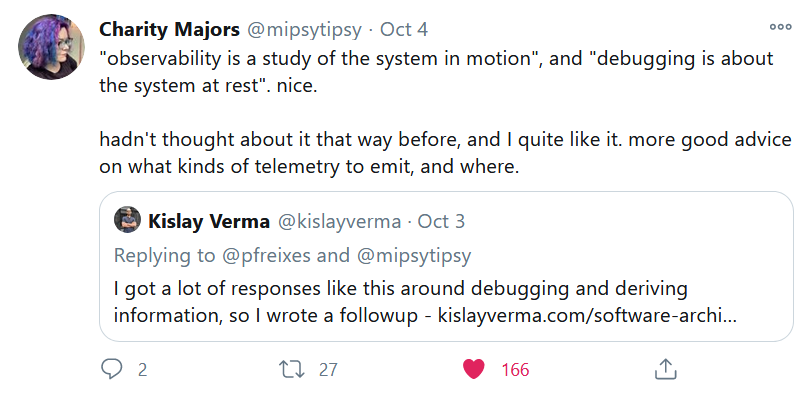
It took me a while to figure out what observability was all about. A year or two I asked around and my colleagues told me that I needed to follow Charity Majors and to read her blog (done, and done). Just this week, Charity tweeted:

Kislay’s tweet led to his blog post, Observing is not Debugging, which I found very helpful. As Charity noted, Kislay tells us that Observability is a study of the system in motion.

Today’s large-scale distributed applications and systems are effectively always in motion. Whether serving web requests, processing streams of data or handling events, something is always happening. At world-scale, looking at individual requests or events is not always feasible. Instead, it is necessary to take a statistical approach and to watch how well a system is working, instead of simply waiting for a total failure.

New AWS Distro for OpenTelemetry
Today we are launching a preview of AWS Distro for OpenTelemetry. We are part of the Cloud Native Computing Foundation (CNCF)’s OpenTelemetry community, working to define an open standard for the collection of distributed traces and metrics. AWS Distro for OpenTelemetry is a secure and supported distribution of the APIs, libraries, agents, and collectors defined in the OpenTelemetry Specification.

One of the coolest features of the toolkit is auto instrumentation. Starting with Java and in the works for other languages and environments (.NET and JavaScript are next), the auto-instrumentation agent identifies the frameworks and languages used by your application and automatically instruments them to collect and forward metrics and traces.

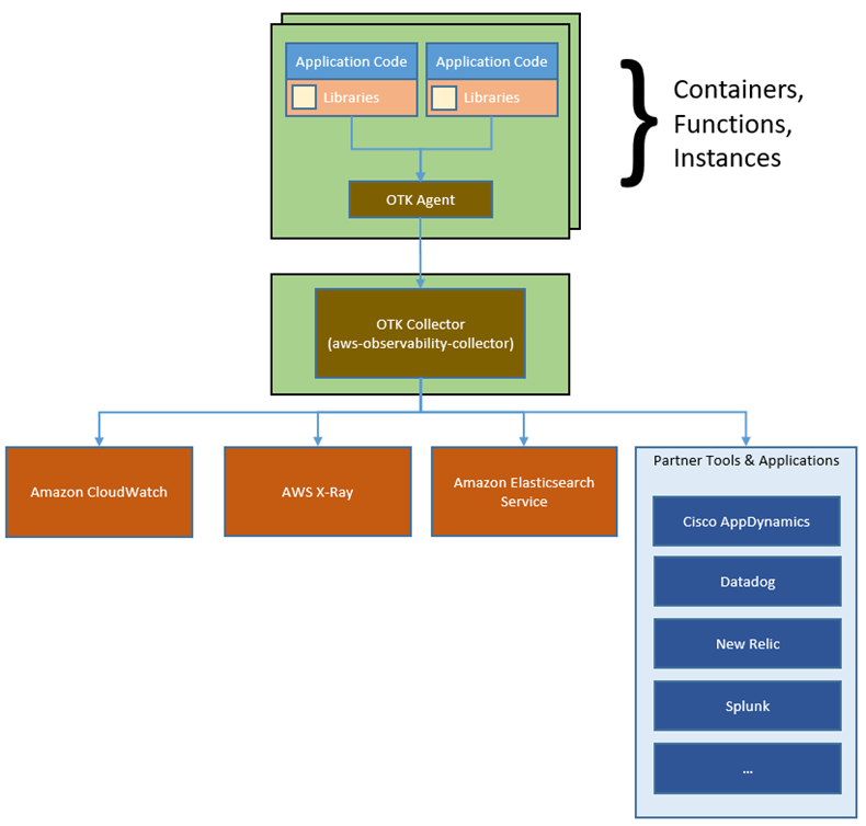
Here’s how all of the pieces fit together:

The AWS Observability Collector runs within your environment. It can be launched as a sidecar or daemonset for EKS, a sidecar for ECS, or an agent on EC2. You configure the metrics and traces that you want to collect, and also which AWS services to forward them to. You can set up a central account for monitoring complex multi-account applications, and you can also control the sampling rate (what percentage of the raw data is forwarded and ultimately stored).

Partners in Action
You can make use of AWS and partner tools and applications to observe, analyze, and act on what you see. We’re working with Cisco AppDynamics, Datadog, New Relic, Splunk, and other partners and will have more information to share during the preview.

Things to Know
The preview of the AWS Distro for OpenTelemetry is available now and you can start using it today. In addition to the .NET and JavaScript support that I mentioned earlier, we plan to support Python, Ruby, Go, C++, Erlang, and Rust as well.

This is an open source project and welcome your pull requests! We will be tracking the upstream repository and plan to release a fresh version of the toolkit quarterly.

— Jeff;

PS – Be sure to sign up for our upcoming webinar, Observability at AWS and AWS Distro for OpenTelemetry Deep Dive.


New – Amazon RDS on Graviton2 Processors

Post Syndicated from Sébastien Stormacq original https://aws.amazon.com/blogs/aws/new-amazon-rds-on-graviton2-processors/

I recently wrote a post to announce the availability of M6g, R6g and C6g families of instances on Amazon Elastic Compute Cloud (EC2). These instances offer better cost-performance ratio than their x86 counterparts. They are based on AWS-designed AWS Graviton2 processors, utilizing 64-bit Arm Neoverse N1 cores.

Starting today, you can also benefit from better cost-performance for your Amazon Relational Database Service (RDS) databases, compared to the previous M5 and R5 generation of database instance types, with the availability of AWS Graviton2 processors for RDS. You can choose between M6g and R6g instance families and three database engines (MySQL 8.0.17 and higher, MariaDB 10.4.13 and higher, and PostgreSQL 12.3 and higher).

M6g instances are ideal for general purpose workloads. R6g instances offer 50% more memory than their M6g counterparts and are ideal for memory intensive workloads, such as Big Data analytics.

Graviton2 instances provide up to 35% performance improvement and up to 52% price-performance improvement for RDS open source databases, based on internal testing of workloads with varying characteristics of compute and memory requirements.

Graviton2 instances family includes several new performance optimizations such as larger L1 and L2 caches per core, higher Amazon Elastic Block Store (EBS) throughput than comparable x86 instances, fully encrypted RAM, and many others as detailed on this page. You can benefit from these optimizations with minimal effort, by provisioning or migrating your RDS instances today.

RDS instances are available in multiple configurations, starting with 2 vCPUs, with 8 GiB memory for M6g, and 16 GiB memory for R6g with up to 10 Gbps of network bandwidth, giving you new entry-level general purpose and memory optimized instances. The table below shows the list of instance sizes available for you:

Instance Size vCPU Memory (GiB) Dedicated EBS Bandwidth (Mbps) Network Bandwidth
(Gbps)
M6g R6g
large 2 8 16 Up to 4750 Up to 10
xlarge 4 16 32 Up to 4750 Up to 10
2xlarge 8 32 64 Up to 4750 Up to 10
4xlarge 16 64 128 4750 Up to 10
8xlarge 32 128 256 9000 12
12xlarge 48 192 384 13500 20
16xlarge 64 256 512 19000 25

Let’s Start Your First Graviton2 Based Instance
To start a new RDS instance, I use the AWS Management Console or the AWS Command Line Interface (CLI), just like usual, and select one of the db.m6g or db.r6ginstance types (this page in the documentation has all the details).

RDS Launch Graviton2 instance

Using the CLI, it would be:

aws rds create-db-instance
 --region us-west-2 \
 --db-instance-identifier $DB_INSTANCE_NAME \
 --db-instance-class db.m6g.large \
 --engine postgres \
 --engine-version 12.3 \
 --allocated-storage 20 \
 --master-username $MASTER_USER \
 --master-user-password $MASTER_PASSWORD

The CLI confirms with:

{
    "DBInstance": {
        "DBInstanceIdentifier": "newsblog",
        "DBInstanceClass": "db.m6g.large",
        "Engine": "postgres",
        "DBInstanceStatus": "creating",
...
}

Migrating to Graviton2 instances is easy, in the AWS Management Console, I select my database and I click Modify.

Modify RDS database

The I select the new DB instance class:

modify db instance

Or, using the CLI, I can use the modify-db-instance API call.

There is a short service interruption happening when you switch instance type. By default, the modification will happen during your next maintenance window, unless you enable the ApplyImmediately option.

You can provision new or migrate to Graviton2 Amazon Relational Database Service (RDS) instances in all regions where EC2 M6g and R6g are available : US East (N. Virginia), US East (Ohio), US West (Oregon), Asia Pacific (Mumbai), Asia Pacific (Singapore), Asia Pacific (Sydney), Asia Pacific (Tokyo), Europe (Ireland), and Europe (Frankfurt) AWS Regions.

As usual, let us know your feedback on the AWS Forum or through your usual AWS contact.

— seb

New – Redis 6 Compatibility for Amazon ElastiCache

Post Syndicated from Channy Yun original https://aws.amazon.com/blogs/aws/new-redis-6-compatibility-for-amazon-elasticache/

After the last Redis 5.0 compatibility for Amazon ElastiCache, there has been lots of improvements to Amazon ElastiCache for Redis including upstream supports such as 5.0.6.

Earlier this year, we announced Global Datastore for Redis that lets you replicate a cluster in one region to clusters in up to two other regions. Recently we improved your ability to monitor your Redis fleet by enabling 18 additional engine and node-level CloudWatch metrics. Also, we added support for resource-level permission policies, allowing you to assign AWS Identity and Access Management (IAM) principal permissions to specific ElastiCache resource or resources.

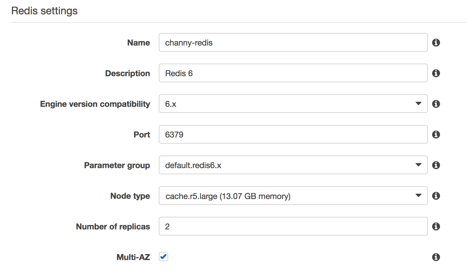
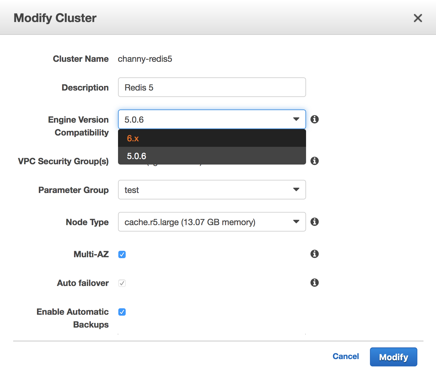
Today, I am happy to announce Redis 6 compatibility to Amazon ElastiCache for Redis. This release brings several new and important features to Amazon ElastiCache for Redis:

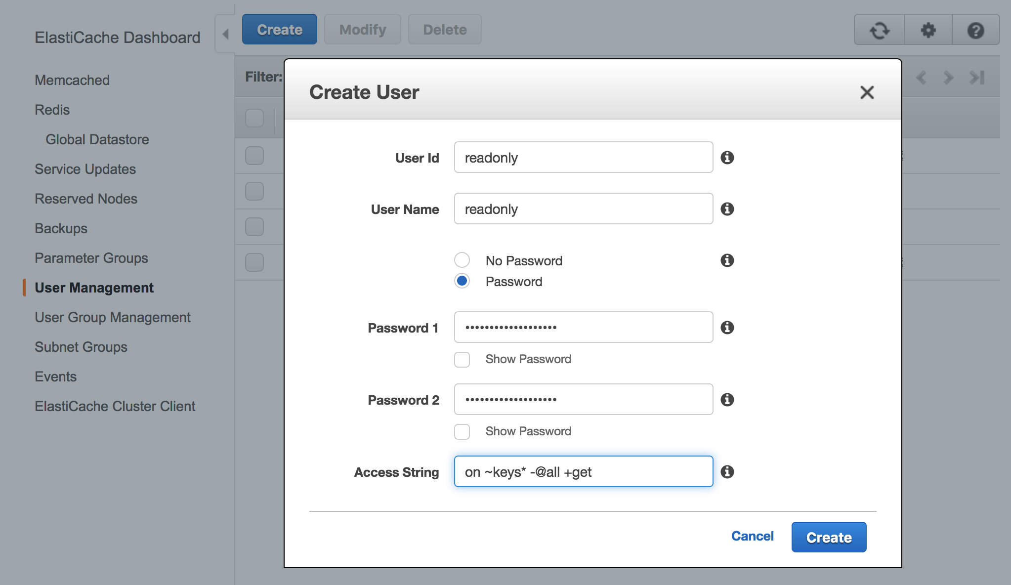
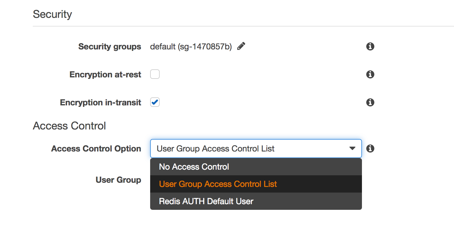
  • Managed Role-Based Access Control – Amazon ElastiCache for Redis 6 now provides you with the ability to create and manage users and user groups that can be used to set up Role-Based Access Control (RBAC) for Redis commands. You can now simplify your architecture while maintaining security boundaries by having several applications use the same Redis cluster without being able to access each other’s data. You can also take advantage of granular access control and authorization to create administration and read-only user groups. Amazon ElastiCache enhances the new Access Control Lists (ACL) introduced in open source Redis 6 to provide a managed RBAC experience, making it easy to set up access control across several Amazon ElastiCache for Redis clusters.
  • Client-Side Caching – Amazon ElastiCache for Redis 6 comes with server-side enhancements to deliver efficient client-side caching to further improve your application performance. Redis clusters now support client-side caching by tracking client requests and sending invalidation messages for data stored on the client. In addition, you can also take advantage of a broadcast mode that allows clients to subscribe to a set of notifications from Redis clusters.
  • Significant Operational Improvements – This release also includes several enhancements that improve application availability and reliability. Specifically, Amazon ElastiCache has improved replication under low memory conditions, especially for workloads with medium/large sized keys, by reducing latency and the time it takes to perform snapshots. Open source Redis enhancements include improvements to expiry algorithm for faster eviction of expired keys and various bug fixes.

Note that open source Redis 6 also announced support for encryption-in-transit, a capability that is already available in Amazon ElastiCache for Redis 4.0.10 onwards. This release of Amazon ElastiCache for Redis 6 does not impact Amazon ElastiCache for Redis’ existing support for encryption-in-transit.

In order to apply RBAC to a new or existing Redis 6 cluster, we first need to ensure you have a user and user group created. We’ll review the process to do this below.

Using Role-Based Access Control – How it works
An alternative to Authenticating Users with the Redis AUTH Command, Amazon ElastiCache for Redis 6 offers Role-Based Access Control (RBAC). With RBAC, you create users and assign them specific permissions via an Access String.

If you want to create, modify, and delete users and user groups, you will need to select to the User Management and User Group Management sections in the ElastiCache console.

ElastiCache will automatically configure a default user with user ID and user name “default”, and then you can add it or new created users to new groups in User Group Management.

If you want to change the default user with your own password and access setting, you need to create a new user with the username set to “default” and can then swap it with the original default user. We recommend using your own strong password for a default user.

The following example shows how to swap the original default user with another default that has a modified access string via AWS CLI.

$ aws elasticache create-user \
 --user-id "new-default-user" \
 --user-name "default" \
 --engine "REDIS" \
 --passwords "a-str0ng-pa))word" \ 
 --access-string "off +get ~keys*"

Create a user group and add the user you created previously.

$ aws elasticache create-user-group \
  --user-group-id "new-default-group" \
  --engine "REDIS" \
  --user-ids "default"

Swap the new default user with the original default user.

$ aws elasticache modify-user-group \
    --user-group-id "new-default-group" \
    --user-ids-to-add "new-default-user" \
    --user-ids-to-remove "default"

Also, you can modify a user’s password or change its access permissions using modify-user command, or remove a specific user using delete-user command. It will be removed from any user groups to which it belongs.

Similarly you can modify a user group by adding new users and/or removing current users using modify-user-group command, or delete a user group using delete-user-group command. Note that the user group itself, not the users belonging to the group, will be deleted.

Once you have created a user group and added users, you can assign the user group to a replication group, or migrate between Redis AUTH and RBAC. For more information, see the documentation in detail.

Redis 6 cluster for ElastiCache – Getting Started
As usual, you can use the ElastiCache Console, CLI, APIs, or a CloudFormation template to create to new Redis 6 cluster. I’ll use the Console, choose Redis from the navigation pane and click Create with the following settings:

Select “Encryption in-transit” checkbox to ensure you can see the “Access Control” options. You can select an option of Access Control either User Group Access Control List by RBAC features or Redis AUTH default user. If you select RBAC, you can choose one of the available user groups.

My cluster is up and running within minutes. You can also use the in-place upgrade feature on existing cluster. By selecting the cluster, click Action and Modify. You can change the Engine Version from 5.0.6-compatible engine to 6.x.

Now Available
Amazon ElastiCache for Redis 6 is now available in all AWS regions. For a list of ElastiCache for Redis supported versions, refer to the documentation. Please send us feedback either in the AWS forum for Amazon ElastiCache or through AWS support, or your account team.

– Channy;

Amazon S3 Update – Three New Security & Access Control Features

Post Syndicated from Jeff Barr original https://aws.amazon.com/blogs/aws/amazon-s3-update-three-new-security-access-control-features/

A year or so after we launched Amazon S3, I was in an elevator at a tech conference and heard a couple of developers use “just throw it into S3” as the answer to their data storage challenge. I remember that moment well because the comment was made so casually, and it was one of the first times that I fully grasped just how quickly S3 had caught on.

Since that launch, we have added hundreds of features and multiple storage classes to S3, while also reducing the cost to storage a gigabyte of data for a month by almost 85% (from $0.15 to $0.023 for S3 Standard, and as low as $0.00099 for S3 Glacier Deep Archive). Today, our customers use S3 to support many different use cases including data lakes, backup and restore, disaster recovery, archiving, and cloud-native applications.

Security & Access Control
As the set of use cases for S3 has expanded, our customers have asked us for new ways to regulate access to their mission-critical buckets and objects. We added IAM policies many years ago, and Block Public Access in 2018. Last year we added S3 Access Points (Easily Manage Shared Data Sets with Amazon S3 Access Points) to help you manage access in large-scale environments that might encompass hundreds of applications and petabytes of storage.

Today we are launching S3 Object Ownership as a follow-on to two other S3 security & access control features that we launched earlier this month. All three features are designed to give you even more control and flexibility:

Object Ownership – You can now ensure that newly created objects within a bucket have the same owner as the bucket.

Bucket Owner Condition – You can now confirm the ownership of a bucket when you create a new object or perform other S3 operations.

Copy API via Access Points – You can now access S3’s Copy API through an Access Point.

You can use all of these new features in all AWS regions at no additional charge. Let’s take a look at each one!

Object Ownership
With the proper permissions in place, S3 already allows multiple AWS accounts to upload objects to the same bucket, with each account retaining ownership and control over the objects. This many-to-one upload model can be handy when using a bucket as a data lake or another type of data repository. Internal teams or external partners can all contribute to the creation of large-scale centralized resources. With this model, the bucket owner does not have full control over the objects in the bucket and cannot use bucket policies to share objects, which can lead to confusion.

You can now use a new per-bucket setting to enforce uniform object ownership within a bucket. This will simplify many applications, and will obviate the need for the Lambda-powered self-COPY that has become a popular way to do this up until now. Because this setting changes the behavior seen by the account that is uploading, the PUT request must include the bucket-owner-full-control ACL. You can also choose to use a bucket policy that requires the inclusion of this ACL.

To get started, open the S3 Console, locate the bucket and view its Permissions, click Object Ownership, and Edit:

Then select Bucket owner preferred and click Save:

As I mentioned earlier, you can use a bucket policy to enforce object ownership (read About Object Ownership and this Knowledge Center Article to learn more).

Many AWS services deliver data to the bucket of your choice, and are now equipped to take advantage of this feature. S3 Server Access Logging, S3 Inventory, S3 Storage Class Analysis, AWS CloudTrail, and AWS Config now deliver data that you own. You can also configure Amazon EMR to use this feature by setting fs.s3.canned.acl to BucketOwnerFullControl in the cluster configuration (learn more).

Keep in mind that this feature does not change the ownership of existing objects. Also, note that you will now own more S3 objects than before, which may cause changes to the numbers you see in your reports and other metrics.

AWS CloudFormation support for Object Ownership is under development and is expected to be ready before AWS re:Invent.

Bucket Owner Condition
This feature lets you confirm that you are writing to a bucket that you own.

You simply pass a numeric AWS Account ID to any of the S3 Bucket or Object APIs using the expectedBucketOwner parameter or the x-amz-expected-bucket-owner HTTP header. The ID indicates the AWS Account that you believe owns the subject bucket. If there’s a match, then the request will proceed as normal. If not, it will fail with a 403 status code.

To learn more, read Bucket Owner Condition.

Copy API via Access Points
S3 Access Points give you fine-grained control over access to your shared data sets. Instead of managing a single and possibly complex policy on a bucket, you can create an access point for each application, and then use an IAM policy to regulate the S3 operations that are made via the access point (read Easily Manage Shared Data Sets with Amazon S3 Access Points to see how they work).

You can now use S3 Access Points in conjunction with the S3 CopyObject API by using the ARN of the access point instead of the bucket name (read Using Access Points to learn more).

Use Them Today
As I mentioned earlier, you can use all of these new features in all AWS regions at no additional charge.

— Jeff;


Store and Access Time Series Data at Any Scale with Amazon Timestream – Now Generally Available

Post Syndicated from Danilo Poccia original https://aws.amazon.com/blogs/aws/store-and-access-time-series-data-at-any-scale-with-amazon-timestream-now-generally-available/

Time series are a very common data format that describes how things change over time. Some of the most common sources are industrial machines and IoT devices, IT infrastructure stacks (such as hardware, software, and networking components), and applications that share their results over time. Managing time series data efficiently is not easy because the data model doesn’t fit general-purpose databases.

For this reason, I am happy to share that Amazon Timestream is now generally available. Timestream is a fast, scalable, and serverless time series database service that makes it easy to collect, store, and process trillions of time series events per day up to 1,000 times faster and at as little as to 1/10th the cost of a relational database.

This is made possible by the way Timestream is managing data: recent data is kept in memory and historical data is moved to cost-optimized storage based on a retention policy you define. All data is always automatically replicated across multiple availability zones (AZ) in the same AWS region. New data is written to the memory store, where data is replicated across three AZs before returning success of the operation. Data replication is quorum based such that the loss of nodes, or an entire AZ, does not disrupt durability or availability. In addition, data in the memory store is continuously backed up to Amazon Simple Storage Service (S3) as an extra precaution.

Queries automatically access and combine recent and historical data across tiers without the need to specify the storage location, and support time series-specific functionalities to help you identify trends and patterns in data in near real time.

There are no upfront costs, you pay only for the data you write, store, or query. Based on the load, Timestream automatically scales up or down to adjust capacity, without the need to manage the underlying infrastructure.

Timestream integrates with popular services for data collection, visualization, and machine learning, making it easy to use with existing and new applications. For example, you can ingest data directly from AWS IoT Core, Amazon Kinesis Data Analytics for Apache Flink, AWS IoT Greengrass, and Amazon MSK. You can visualize data stored in Timestream from Amazon QuickSight, and use Amazon SageMaker to apply machine learning algorithms to time series data, for example for anomaly detection. You can use Timestream fine-grained AWS Identity and Access Management (IAM) permissions to easily ingest or query data from an AWS Lambda function. We are providing the tools to use Timestream with open source platforms such as Apache Kafka, Telegraf, Prometheus, and Grafana.

Using Amazon Timestream from the Console
In the Timestream console, I select Create database. I can choose to create a Standard database or a Sample database populated with sample data. I proceed with a standard database and I name it MyDatabase.

All Timestream data is encrypted by default. I use the default master key, but you can use a customer managed key that you created using AWS Key Management Service (KMS). In that way, you can control the rotation of the master key, and who has permissions to use or manage it.

I complete the creation of the database. Now my database is empty. I select Create table and name it MyTable.

Each table has its own data retention policy. First data is ingested in the memory store, where it can be stored from a minimum of one hour to a maximum of a year. After that, it is automatically moved to the magnetic store, where it can be kept up from a minimum of one day to a maximum of 200 years, after which it is deleted. In my case, I select 1 hour of memory store retention and 5 years of magnetic store retention.

When writing data in Timestream, you cannot insert data that is older than the retention period of the memory store. For example, in my case I will not be able to insert records older than 1 hour. Similarly, you cannot insert data with a future timestamp.

I complete the creation of the table. As you noticed, I was not asked for a data schema. Timestream will automatically infer that as data is ingested. Now, let’s put some data in the table!

Loading Data in Amazon Timestream
Each record in a Timestream table is a single data point in the time series and contains:

  • The measure name, type, and value. Each record can contain a single measure, but different measure names and types can be stored in the same table.
  • The timestamp of when the measure was collected, with nanosecond granularity.
  • Zero or more dimensions that describe the measure and can be used to filter or aggregate data. Records in a table can have different dimensions.

For example, let’s build a simple monitoring application collecting CPU, memory, swap, and disk usage from a server. Each server is identified by a hostname and has a location expressed as a country and a city.

In this case, the dimensions would be the same for all records:

  • country
  • city
  • hostname

Records in the table are going to measure different things. The measure names I use are:

  • cpu_utilization
  • memory_utilization
  • swap_utilization
  • disk_utilization

Measure type is DOUBLE for all of them.

For the monitoring application, I am using Python. To collect monitoring information I use the psutil module that I can install with:

pip3 install psutil

Here’s the code for the collect.py application:

import time
import boto3
import psutil

from botocore.config import Config

DATABASE_NAME = "MyDatabase"
TABLE_NAME = "MyTable"

COUNTRY = "UK"
CITY = "London"
HOSTNAME = "MyHostname" # You can make it dynamic using socket.gethostname()

INTERVAL = 1 # Seconds

def prepare_record(measure_name, measure_value):
    record = {
        'Time': str(current_time),
        'Dimensions': dimensions,
        'MeasureName': measure_name,
        'MeasureValue': str(measure_value),
        'MeasureValueType': 'DOUBLE'
    }
    return record


def write_records(records):
    try:
        result = write_client.write_records(DatabaseName=DATABASE_NAME,
                                            TableName=TABLE_NAME,
                                            Records=records,
                                            CommonAttributes={})
        status = result['ResponseMetadata']['HTTPStatusCode']
        print("Processed %d records. WriteRecords Status: %s" %
              (len(records), status))
    except Exception as err:
        print("Error:", err)


if __name__ == '__main__':

    session = boto3.Session()
    write_client = session.client('timestream-write', config=Config(
        read_timeout=20, max_pool_connections=5000, retries={'max_attempts': 10}))
    query_client = session.client('timestream-query')

    dimensions = [
        {'Name': 'country', 'Value': COUNTRY},
        {'Name': 'city', 'Value': CITY},
        {'Name': 'hostname', 'Value': HOSTNAME},
    ]

    records = []

    while True:

        current_time = int(time.time() * 1000)
        cpu_utilization = psutil.cpu_percent()
        memory_utilization = psutil.virtual_memory().percent
        swap_utilization = psutil.swap_memory().percent
        disk_utilization = psutil.disk_usage('/').percent

        records.append(prepare_record('cpu_utilization', cpu_utilization))
        records.append(prepare_record(
            'memory_utilization', memory_utilization))
        records.append(prepare_record('swap_utilization', swap_utilization))
        records.append(prepare_record('disk_utilization', disk_utilization))

        print("records {} - cpu {} - memory {} - swap {} - disk {}".format(
            len(records), cpu_utilization, memory_utilization,
            swap_utilization, disk_utilization))

        if len(records) == 100:
            write_records(records)
            records = []

        time.sleep(INTERVAL)

I start the collect.py application. Every 100 records, data is written in the MyData table:

$ python3 collect.py
records 4 - cpu 31.6 - memory 65.3 - swap 73.8 - disk 5.7
records 8 - cpu 18.3 - memory 64.9 - swap 73.8 - disk 5.7
records 12 - cpu 15.1 - memory 64.8 - swap 73.8 - disk 5.7
. . .
records 96 - cpu 44.1 - memory 64.2 - swap 73.8 - disk 5.7
records 100 - cpu 46.8 - memory 64.1 - swap 73.8 - disk 5.7
Processed 100 records. WriteRecords Status: 200
records 4 - cpu 36.3 - memory 64.1 - swap 73.8 - disk 5.7
records 8 - cpu 31.7 - memory 64.1 - swap 73.8 - disk 5.7
records 12 - cpu 38.8 - memory 64.1 - swap 73.8 - disk 5.7
. . .

Now, in the Timestream console, I see the schema of the MyData table, automatically updated based on the data ingested:

Note that, since all measures in the table are of type DOUBLE, the measure_value::double column contains the value for all of them. If the measures were of different types (for example, INT or BIGINT) I would have more columns (such as measure_value::int and measure_value::bigint) .

In the console, I can also see a recap of which kind measures I have in the table, their corresponding data type, and the dimensions used for that specific measure:

Querying Data from the Console
I can query time series data using SQL. The memory store is optimized for fast point-in-time queries, while the magnetic store is optimized for fast analytical queries. However, queries automatically process data on all stores (memory and magnetic) without having to specify the data location in the query.

I am running queries straight from the console, but I can also use JDBC connectivity to access the query engine. I start with a basic query to see the most recent records in the table:

SELECT * FROM MyDatabase.MyTable ORDER BY time DESC LIMIT 8

Let’s try something a little more complex. I want to see the average CPU utilization aggregated by hostname in 5 minutes intervals for the last two hours. I filter records based on the content of measure_name. I use the function bin() to round time to a multiple of an interval size, and the function ago() to compare timestamps:

SELECT hostname,
       bin(time, 5m) as binned_time,
       avg(measure_value::double) as avg_cpu_utilization
  FROM MyDatabase.MyTable
 WHERE measure_name = 'cpu_utilization'
   AND time > ago(2h)
 GROUP BY hostname, bin(time, 5m)

When collecting time series data you may miss some values. This is quite common especially for distributed architectures and IoT devices. Timestream has some interesting functions that you can use to fill in the missing values, for example using linear interpolation, or based on the last observation carried forward.

More generally, Timestream offers many functions that help you to use mathematical expressions, manipulate strings, arrays, and date/time values, use regular expressions, and work with aggregations/windows.

To experience what you can do with Timestream, you can create a sample database and add the two IoT and DevOps datasets that we provide. Then, in the console query interface, look at the sample queries to get a glimpse of some of the more advanced functionalities:

Using Amazon Timestream with Grafana
One of the most interesting aspects of Timestream is the integration with many platforms. For example, you can visualize your time series data and create alerts using Grafana 7.1 or higher. The Timestream plugin is part of the open source edition of Grafana.

I add a new GrafanaDemo table to my database, and use another sample application to continuously ingest data. The application simulates performance data collected from a microservice architecture running on thousands of hosts.

I install Grafana on an Amazon Elastic Compute Cloud (EC2) instance and add the Timestream plugin using the Grafana CLI.

$ grafana-cli plugins install grafana-timestream-datasource

I use SSH Port Forwarding to access the Grafana console from my laptop:

$ ssh -L 3000:<EC2-Public-DNS>:3000 -N -f ec2-user@<EC2-Public-DNS>

In the Grafana console, I configure the plugin with the right AWS credentials, and the Timestream database and table. Now, I can select the sample dashboard, distributed as part of the Timestream plugin, using data from the GrafanaDemo table where performance data is continuously collected:

Available Now
Amazon Timestream is available today in US East (N. Virginia), Europe (Ireland), US West (Oregon), and US East (Ohio). You can use Timestream with the console, the AWS Command Line Interface (CLI), AWS SDKs, and AWS CloudFormation. With Timestream, you pay based on the number of writes, the data scanned by the queries, and the storage used. For more information, please see the pricing page.

You can find more sample applications in this repo. To learn more, please see the documentation. It’s never been easier to work with time series, including data ingestion, retention, access, and storage tiering. Let me know what you are going to build!

— Danilo