Post Syndicated from Zhe Cheng original https://blog.zabbix.com/next-level-alert-analysis-with-deepseek-and-zabbix/30424/
As IT infrastructures grow increasingly complex, efficiently analyzing monitoring data and accelerating incident response have become critical challenges for operations teams. This post explores a few innovative applications of DeepSeek when integrated with Zabbix.

Requirements:
– Zabbix server 7.0 or higher
– DeepSeek API (Alternatively, other AI APIs can be used if needed)
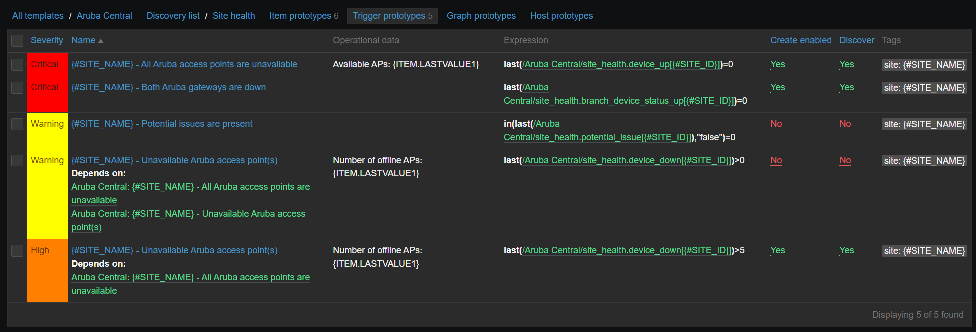
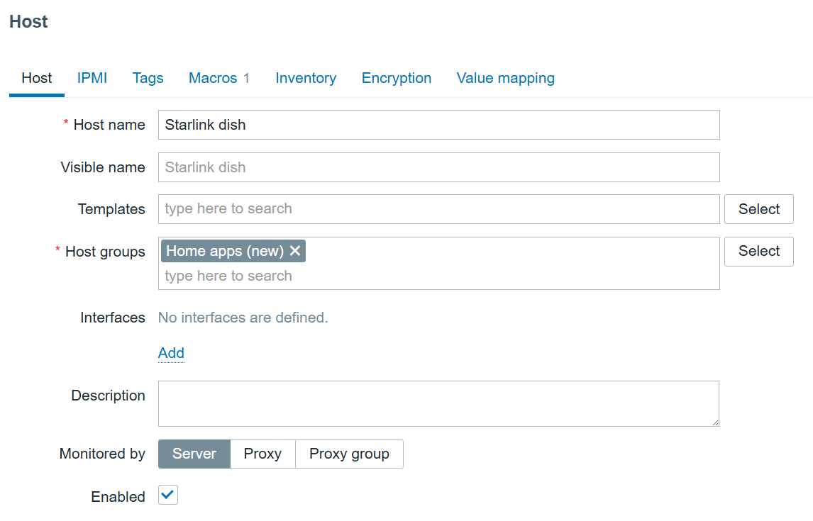
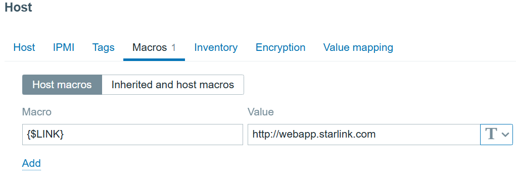
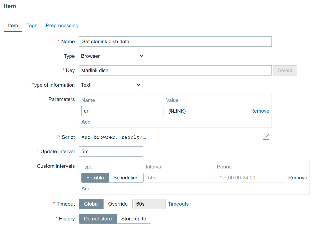
1. Scenario One: One-Click Intelligent Alert Analysis
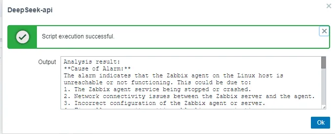
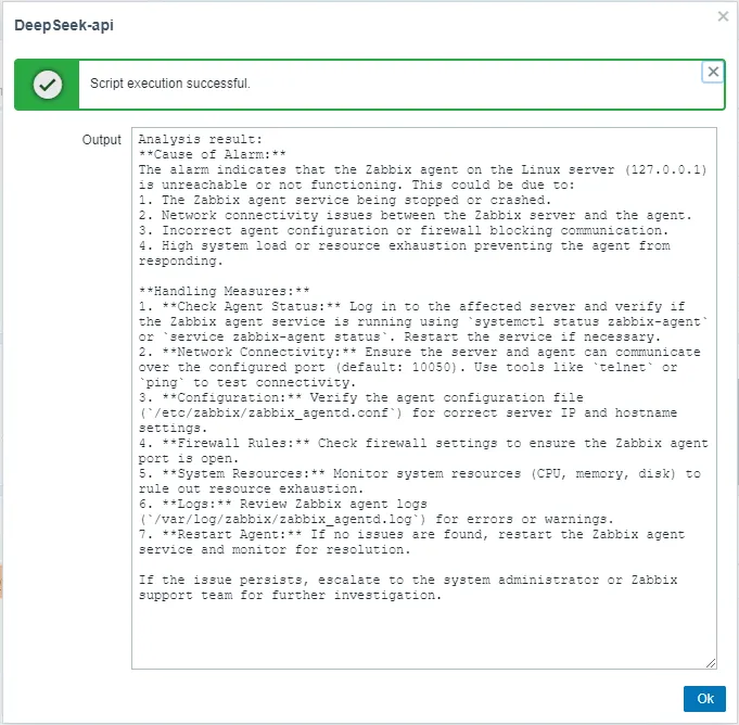
By integrating DeepSeek Analytics into the Zabbix frontend, users can conduct intelligent alert analysis with just one click. This integration facilitates the swift generation of comprehensive fault analyses and solution suggestions, markedly decreasing the MTTR (Mean Time to Resolution). Consequently, it streamlines the troubleshooting process, alleviates the workload on IT personnel, ensures system stability, and conserves both time and resources.
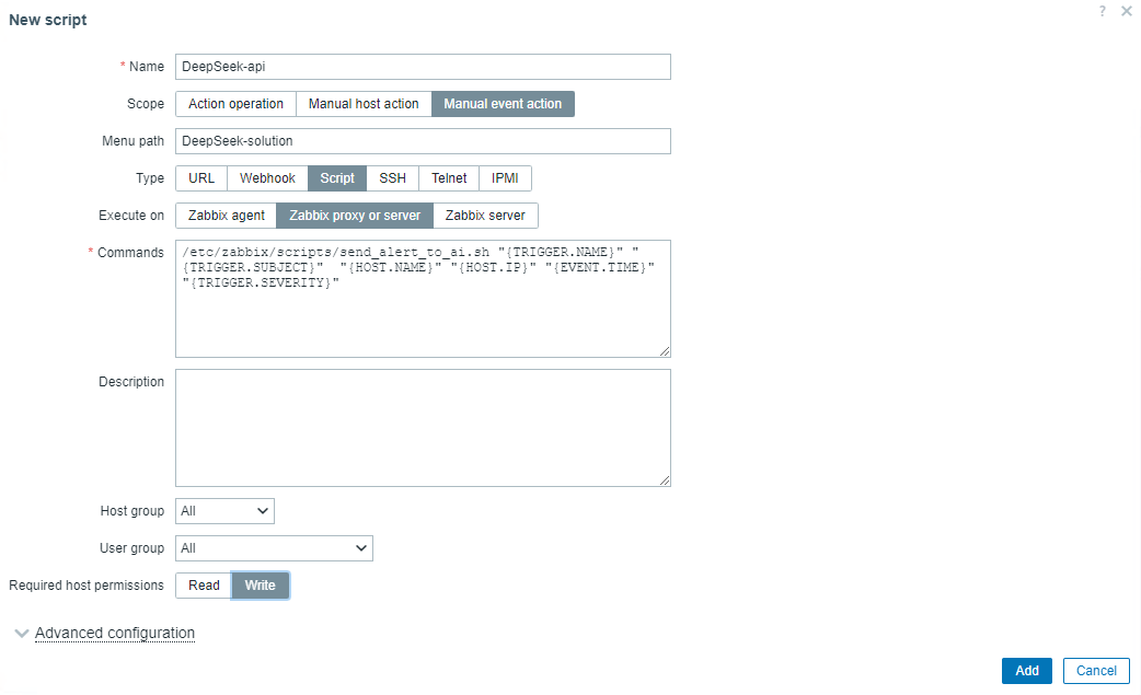
1.1 On the Zabbix home page, navigate to “Alerts” > “Scripts”, and click on the “Create script” button.
1.2 Configuration script:
- Name: Can be customized
- Scope: Select “Manual event action”
- Menu path: Customize menu paths for quick access
- Type: Select “Script”
- Execute on: Select “Zabbix proxy or server”
1.3 Enter the following command in the command bar:
/etc/zabbix/scripts/send_alert_to_ai.sh "{TRIGGER.NAME}" "{TRIGGER.SUBJECT}" "{HOST.NAME}" "{HOST.IP}" "{EVENT.TIME}" "{TRIGGER.SEVERITY}"

1.4 Create an API call script on zabbix-server.
1.4.1 Modify the Zabbix Server Configuration File and Enable Global Scripts:
Open the Zabbix server configuration file for editing:
vi /etc/zabbix/zabbix_server.conf
Set the EnableGlobalScripts option to 1:
EnableGlobalScripts=1
Save the changes and exit the editor. Then, restart the Zabbix server service to apply the changes:
systemctl restart zabbix-server
1.4.2 Create an API Call Script.
Create a directory for custom scripts if it does not already exist:
mkdir -p /etc/zabbix/scripts && cd /etc/zabbix/scripts
Note: If the frontend prompts that the script file cannot be found, try moving the script to the directory used by the Nginx agent. Create a new script file named send_alert_to_ai.sh:
vi send_alert_to_ai.sh
Add the following content to the script, replacing DeepSeek KEY with your actual API key. Make sure you adjust the API call method if using a different AI service:
#!/bin/bash

# DeepSeek API configuration
API_URL="https://api.deepseek.com/chat/completions"
API_KEY="xxxxxxxxxxxxxxxxxxxx"

# Obtain the parameters to be passed as alarm information
TRIGGER_NAME="$1"
ALERT_SUBJECT="$2"
HOSTNAME="$3"
HOST_IP="$4"
EVENT_TIME="$5"
TRIGGER_SEVERITY="$6"

# Build a more concise JSON format for alarm information
alert_info=$(cat <<EOF
{
"model": "deepseek-chat",
"messages": [
{"role": "system", "content": "You are an assistant focused on responding quickly to system alarms。"},
{"role": "user", "content": "The following alarm information is received:\n\n: $TRIGGER_NAME\n: $ALERT_SUBJECT\n: $HOSTNAME\n: $HOST_IP\n: $EVENT_TIME\n: $TRIGGER_SEVERITY\n\nPlease tell me the cause of the alarm and the handling measures in a short and professional language with a word limit of 300 words。"}
],
"stream": false
}
EOF
)

# Send the POST request and capture the response and HTTP status code
response=$(curl -s -w "\n%{http_code}" -X POST "$API_URL" \
-H "Content-Type: application/json" \
-H "Authorization: Bearer $API_KEY" \
-d "$alert_info")

# Separate HTTP status codes from response bodies
http_code=$(echo "$response" | tail -n1)
response_body=$(echo "$response" | sed '$d')

# Parse and extract the content field
if [ "$http_code" -eq 200 ]; then
# Parse JSON using the jq tool
if ! command -v jq &> /dev/null; then
echo "jq could not be found, please install it first."
exit 1
fi

# Extract the content field and format the output
content=$(echo "$response_body" | jq -r '.choices[0].message.content')
echo -e "Analysis result:\n$content"
else
echo "failure: HTTP status code $http_code, respond: $response_body"
fi
Make the script executable:
chmod +x send_alert_to_ai.sh
Note: The script provided invokes the official DeepSeek API. Replace DeepSeek KEY with your actual API_KEY. If you are using another AI service, please confirm the appropriate API invocation method.
Important Notes:
Note: The script relies on jq to process and parse JSON data for tasks such as filtering, mapping, aggregating, and formatting. If jq is not installed on your system, follow these instructions to install it.
For Debian/Ubuntu Systems:
apt-get update
apt-get install jq
For CentOS/RHEL Systems:
yum install epel-release
yum install jq
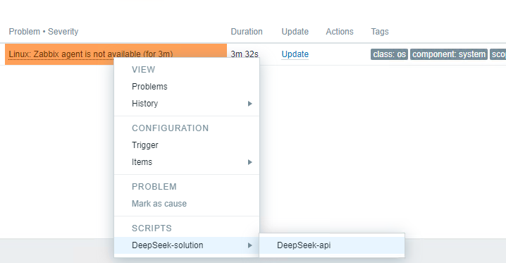
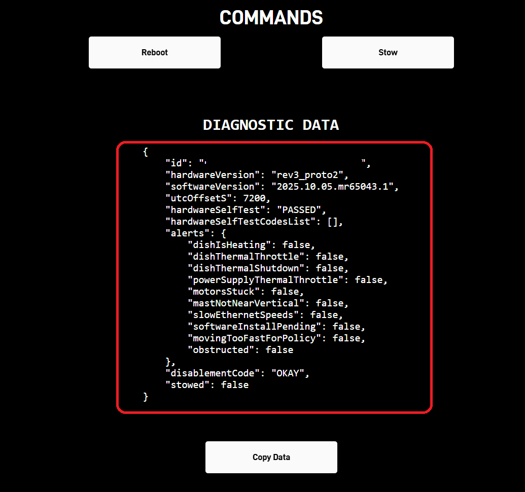
1.5 Actual Effect Display:


1.6 Optional Optimization Items.
1.6.1 Adjust Output Box Size for Better Browsing.
After executing the script, you may find that the output box is too small and inconvenient to browse. To optimize this, you can modify the front-end CSS file as follows.
Back up the existing CSS File:
cd /usr/share/nginx/html/assets/styles/
cp blue-theme.css blue-theme.css.bak
Edit the CSS File:
vi /usr/share/nginx/html/assets/styles/blue-theme.css
Add Custom Styles at the End of the File.
Add the following CSS rules to adjust the size and behavior of the output box:
#execution-output {
height: 500px; /* Adjust to your desired height */
width: 540px; /* Optional: Adjust the width as required */
overflow-y: auto; /* Displays scrollbar when content exceeds the set height */
}
Save and exit the editor. At this point, clear the browser cache and reload the page to see the changes take effect.
1.6.2 How to Optimize Slow Output Response after Executing the One-Click Analysis Script.
During actual testing, it was estimated that returning a 300-word result takes approximately 20 to 30 seconds. While you can improve the response speed by adjusting the preset prompt words in the script, this approach may reduce the richness of the analysis content. Therefore, it is recommended to balance speed and content depth by adjusting the number of replies in the script’s prompt words according to your actual needs.
Actual effect display:

2. Scenario Two: Zabbix Documentation Knowledge Base Assistant
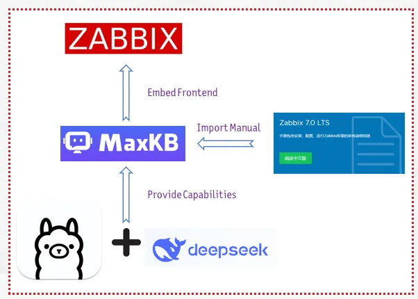
In today’s fast-paced IT environment, managing and retrieving information efficiently is crucial. To address this need, we’ve developed the Zabbix KB Assistant, an intelligent knowledge base solution built on MaxKB—an open-source Q&A system leveraging large language models.
This assistant streamlines access to Zabbix’s extensive documentation, making it easier than ever for users to find the information they require.
MaxKB stands out for its seamless integration capabilities, allowing for quick uploads of documents and automatic crawling of online content.
Its flexibility means it can be effortlessly embedded into third-party systems, including our very own Zabbix platform. The project is available at the GitHub repository.

The development process of Zabbix KB Assistant involved configuring MaxKB to recognize and parse the official Zabbix documentation. By utilizing this URL, we ensured that the latest updates and comprehensive guides are always accessible within our assistant. After setting up the core model configurations, we created a dedicated knowledge base tailored to Zabbix’s rich content.
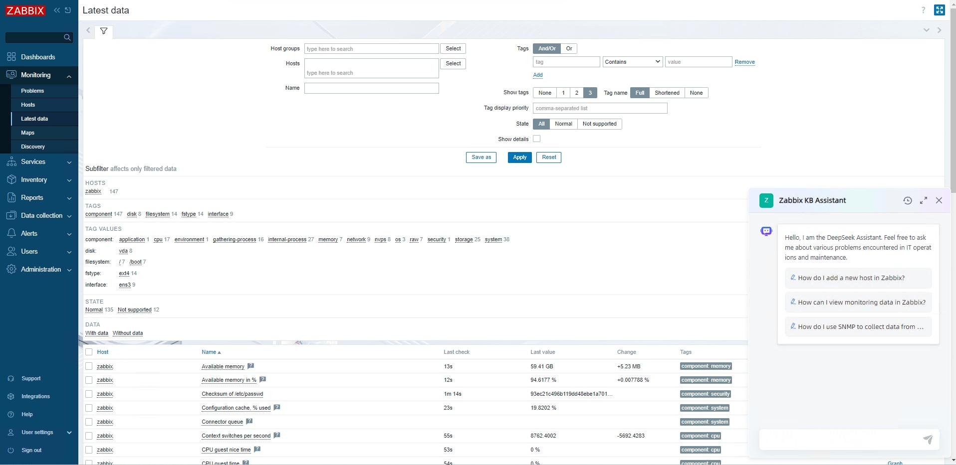
With the knowledge base in place, we proceeded to integrate Zabbix KB Assistant into the Zabbix frontend. This step was essential for providing instant access to users navigating the Zabbix interface. By embedding a floating window mode, users can interact with the assistant without leaving their current page—a feature that significantly enhances user experience.
Actual effect display:
3. Scenario Three: DingTalk Alert Enhancement
By integrating DeepSeek’s deep analysis capabilities, DingTalk can automatically analyze alarm information upon receiving alerts. This integration provides precise fault diagnosis and solutions, aiding IT operations and maintenance personnel in quickly identifying and resolving issues. Consequently, this improves the efficiency of system maintenance and reduces downtime.
3.1 Create a Bot and Configure Security Settings.
First, create a new bot within the DingTalk group and ensure that the keyword “Alarm” is properly configured in the security settings. Next, retrieve the webhook URL for this bot and keep it safe for later use.
3.2 Install Python3 and Necessary Libraries.
Ensure that Python3 along with the required libraries are installed on your system. Depending on your operating system, follow these instructions.
For Ubuntu/Debian systems:
sudo apt update
sudo apt install python3 python3-pip
pip3 install requests
For CentOS/RHEL systems:
sudo dnf install python3
pip3 install requests
3.3 Below is an example script (deepseekdingding.py) located at /usr/lib/zabbix/alertscripts/.
Replace the placeholder webhook URL and DeepSeek API key in the script with your actual values:
#!/usr/bin/env python3
#coding:utf-8
import requests
import sys
import json

class DingTalkBot(object):
    # Send an alarm
    def send_news_message(self, webhook_url, subject, content, ai_response):
        url = webhook_url
        data = {
            "msgtype": "markdown",
            "markdown": {
                "title": subject,
                "text": f"{subject}\n{content}\n\n【DeepSeek analysis】:\n\n{ai_response}"
            }
        }
        headers = {'Content-Type': 'application/json'}
        response = requests.post(url, headers=headers, data=json.dumps(data))
        return response

if __name__ == '__main__':
    WEBHOOK_URL = 'https://oapi.dingtalk.com/robot/send?access_token=224c1ff0c6df60a809b3c5b69b8448486b780d292e9d395ac8fbf84980214e30'  # Webhook
    API_URL = 'https://api.deepseek.com/chat/completions'
    API_KEY = "xxxxxxxxxxxxxxxxxxxx"  # DeepSeek API

    if len(sys.argv) < 3:
        print("Error: Not enough arguments provided.")
        sys.exit(1)

    subject = str(sys.argv[1])
    content = str(sys.argv[2])

    print(f"Received subject: {subject}")
    print(f"Received content: {content}")

    try:
        headers = {
            'Authorization': f'Bearer {API_KEY}',
            'Content-Type': 'application/json',
        }
        payload = {
            "model": "deepseek-chat",  # DeepSeek
            "messages": [
                {"role": "user", "content": f"If you are a professional IT operation and maintenance expert, please tell me the cause of these alarms and handling suggestions in a concise and professional language with a word limit of 100 words{content}"}
            ]
        }
        ai_response = requests.post(API_URL, headers=headers, json=payload)
        ai_response.raise_for_status()
        ai_response_content = ai_response.json().get('choices', [{}])[0].get('message', {}).get('content', '')
    except Exception as e:
        ai_response_content = "\nThe interface call timed out or an error occurred. Please check the configuration and try again"

    bot = DingTalkBot()
    response = bot.send_news_message(WEBHOOK_URL, subject, content, ai_response_content)

    if response.status_code == 200:
        print("successfully")
    else:
        print(f"failed: {response.text}")
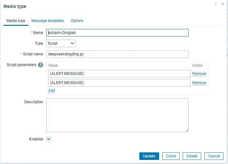
3.5 On the Zabbix home page, go to Alerts – Media types – Create Media type and then enter the following information:
- Name: aiAlarm-Dingtalk
- Type: script
- Script name: deepseekdingding.py
- Script parameter: {ALERT.MESSAGE} {ALERT.SUBJECT}

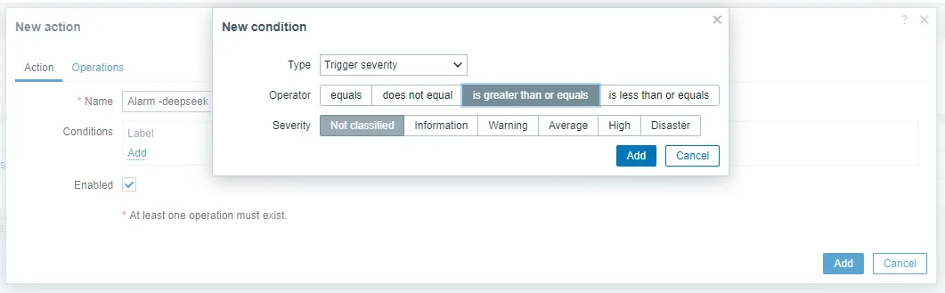
3.6 Create an alarm action.
Go to Alarm – Action – Trigger actions – Create action and set the name to Alarm -deepseek. Select this parameter as required:

Edit the action options as follows:
Send to media type aiAlarm-Dingtalk
Topic fault alarm: {EVENT.NAME}
message
【Zabbix Alarm Notification 】

Alarm group: {TRIGGER.HOSTGROUP.NAME}

Alarm host: {HOSTNAME1}

Alarm time: {EVENT.DATE} {EVENT.TIME}

Alert level: {TRIGGER.SEVERITY}

Problem information: {TRIGGER.NAME}

Confirm the update.
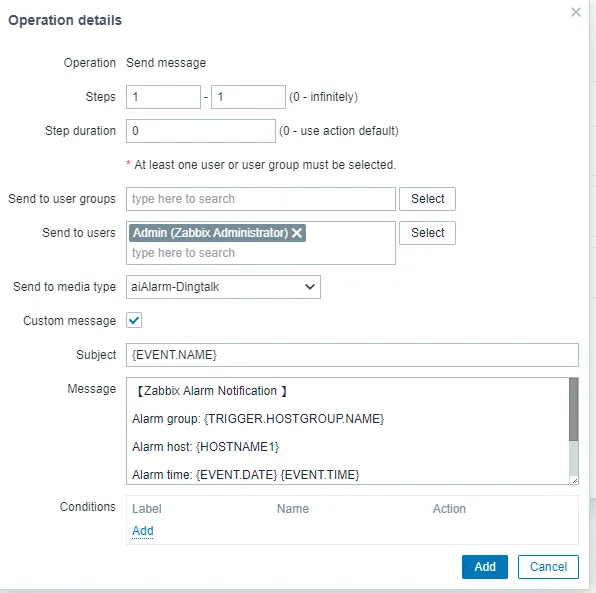
3.7 Configure notification rights for users.
The following item is added to the “User-User-Alarm” media dialog box. Once added, click Update.
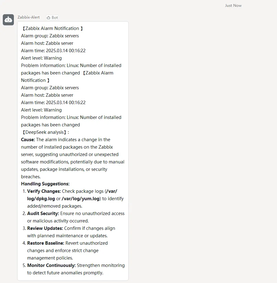
Actual effect display:

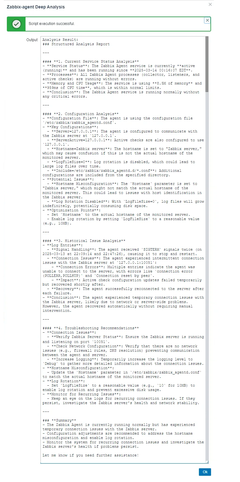
4. Scenario Four: One-Click System Service Deep Analysis
Our solution integrates DeepSeek analysis to offer a one-click intelligent inspection tool that automates the collection of service configurations, logs, and status from within your system. This information is then sent via API to DeepSeek for comprehensive analysis.
Our approach begins by extracting relevant configuration data, recent log entries, and current service statuses. These pieces of information are combined with predefined prompts and submitted to DeepSeek through its API. For instance, a prompt might look like this:
“Here are the current logs for XXX service:\n\n${recent_logs}\n\nService. Status is as follows:\n${service_status}\n. Please analyze the following four aspects based on this information and provide a concise report within 500 words: service status analysis, configuration review, historical issue examination, and troubleshooting recommendations.”
DeepSeek processes this input to perform a detailed breakdown across these four areas, delivering structured feedback and actionable insights.
This integration offers deep system analysis and precise optimization suggestions, enabling swift responses to system changes or anomalies. It aids administrators in promptly identifying and addressing issues.
In addition, it’s easily integrated into existing monitoring systems, allowing adjustments to the depth and scope of analysis as needed. The solution boasts high scalability and flexibility, catering to evolving business requirements.
Actual effect display :

The post Next-Level Alert Analysis with DeepSeek and Zabbix appeared first on Zabbix Blog.


 Never expose your keys publicly!