Tag Archives: news

Introducing Amazon SageMaker Data Wrangler, a Visual Interface to Prepare Data for Machine Learning

Post Syndicated from Julien Simon original https://aws.amazon.com/blogs/aws/introducing-amazon-sagemaker-data-wrangler-a-visual-interface-to-prepare-data-for-machine-learning/

Today, I’m extremely happy to announce Amazon SageMaker Data Wrangler, a new capability of Amazon SageMaker that makes it faster for data scientists and engineers to prepare data for machine learning (ML) applications by using a visual interface.

Whenever I ask a group of data scientists and ML engineers how much time they actually spend studying ML problems, I often hear a collective sigh, followed by something along the lines of, “20%, if we’re lucky.” When I ask them why, the answer is invariably the same, “data preparation consistently takes up to 80% of our time!”

Indeed, preparing data for training is a crucial step of the ML process, and no one would think about botching it up. Typical tasks include:

  • Locating data: finding where raw data is stored, and getting access to it
  • Data visualization: examining statistical properties for each column in the dataset, building histograms, studying outliers
  • Data cleaning: removing duplicates, dropping or filling entries with missing values, removing outliers
  • Data enrichment and feature engineering: processing columns to build more expressive features, selecting a subset of features for training

In the early stage of a new ML project, this is a highly manual process, where intuition and experience play a large part. Using a mix of bespoke tools and open source tools such as pandas or PySpark, data scientists often experiment with different combinations of data transformations, and use them to process datasets before training models. Then, they analyze prediction results and iterate. As important as this is, looping through this process again and again can be time-consuming, tedious, and error-prone.

At some point, you will hit the right level of accuracy (or whatever other metric you’ve picked), and you’ll then want to train on the full dataset in your production environment. However, you’ll first have to reproduce and automate the exact data preparation steps that you experimented within your sandbox. Unfortunately, there’s always room for error given the interactive nature of this work, even if you carefully document it.

Last but not least, you’ll have to manage and scale your data processing infrastructure before you get to the finish line. Now that I think of it, 80% of your time may not be enough to do all of this!

Introducing Amazon SageMaker Data Wrangler
Amazon SageMaker Data Wrangler is integrated in Amazon SageMaker Studio, our fully managed integrated development environment (IDE) for ML. With just a few clicks, you can connect to data sources, explore and visualize data, apply built-in transformations as well as your own, export the resulting code to an auto-generated script, and run it on managed infrastructure. Let’s look at each step in more detail.

Obviously, data preparation starts with locating and accessing data. Out of the box, SageMaker Data Wrangler lets you easily and quickly connect to Amazon Simple Storage Service (S3), Amazon Athena, Amazon Redshift and AWS Lake Formation. You can also import data from Amazon SageMaker Feature Store. As all things AWS, access management is governed by AWS Identity and Access Management (IAM), based on the permissions attached to your SageMaker Studio instance.

Once you’ve connected to your data sources, you’ll probably want to visualize your data. Using the SageMaker Data Wrangler user interface, you can view table summaries, histograms, and scatter plots in seconds. You can also build your own custom graphs by simply copying and running code written with the popular Altair open source library.

Once you’ve got a good grasp on what your data looks like, it’s time to start preparing it. SageMaker Data Wrangler includes 300+ built-in transformations, such as finding and replacing data, splitting/renaming/dropping columns, scaling numerical values, encoding categorical values, and so on. All you have to do is select the transformation in a drop-down list, and fill in the parameters it may require. You can then preview the change, and decide whether you’d like to add it or not to the list of preparation steps for this dataset. If you’d like, you can also add your own code to implement custom transformations, using either pandas, PySpark, or PySpark SQL.

As you add transformation steps to your processing pipeline, you can view its graphical summary in SageMaker Studio. You can also add new stages to the pipeline, for example a new data source, or another group of transformation steps (say, a data cleaning group, followed by a feature engineering group). Thanks to the intuitive user interface, your data preparation pipeline will take shape in front of your eyes, and you’ll instantly be able to check that processed data looks the way that it should.

Early on, you’d certainly love to check your data preparation steps, and also get a sense of their predictive power, wouldn’t you? Good news, then! For regression and classification problem types, the “Quick model” capability lets you select a subset of your data, train a model, and determine which features are contributing most to the predicted outcome. Looking at the model, you can easily diagnose and fix data preparation issues as early as possible, and to determine if additional feature engineering is needed to improve your model performance.

Once you’re happy with your pipeline, you can export it in one click to a Python script that faithfully reproduces your manual steps. You won’t waste any time chasing discrepancies, and you can directly add this code to your ML project.

In addition, you can also export your processing code to:

Now, let’s do a quick demo, and show you how easy it is to work with SageMaker Data Wrangler .

Using Amazon SageMaker Data Wrangler
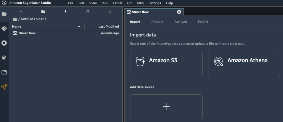
Opening SageMaker Studio, I create a new data flow in order to process the Titanic dataset, which contains information on passengers, and labels showing whether they survived the wreck or not.

SageMaker screenshot

My dataset is stored as a CSV file in Amazon Simple Storage Service (S3), and I select the appropriate data source.

SageMaker screenshot

Using the built-in tool, I quickly navigate my S3 buckets, and I locate the CSV file containing my data. For larger datasets, SageMaker Data Wrangler also supports the Parquet format.

As I select my file, SageMaker Data Wrangler shows me the first few rows.

SageMaker screenshot

I import the dataset, and I’m presented with an initial view of the data flow. Right-clicking on the dataset, I select “Edit data types” to make sure that SageMaker Data Wrangler has correctly detected the type of each column in the dataset.

SageMaker screenshot

Checking each column, it looks like all types are correct.

SageMaker screenshot

Moving back to the data flow view, I select “Add analysis” this time. This opens a new view where I can visualize data using histograms, scatterplots, and more. For example, I build an histogram showing me the age distribution of passengers according to their survival status, and coloring the bins using their gender. Of course, I can save it for future use.

SageMaker screenshot

Moving back to the data flow view once again, I select “Add transform” in order to start processing the dataset. This opens a new view, showing me the first lines of the dataset, as well as a list of 300+ built-in transforms.

SageMaker screenshot

Pclass, the passenger class, is a categorical variable, and I decide to encode it using one-hot encoding. This creates 3 new columns representing different dimensions, and I can preview them. As this is exactly what I wanted, I apply this transform for good. Likewise, I apply the same transform to the Sex column.

SageMaker screenshot

Then, I drop the original Pclass column. Using the same transform, I also drop the Name column.

SageMaker screenshot

In order to get a quick idea on whether these transformations increase or decrease the accuracy of the model, I can create a analysis that trains a model on the spot. As my problem is a binary classification problem, SageMaker Data Wrangler uses a metric called the F1 score. 0.749 is a good start, and additional processing would certainly improve it. I can also see which features contribute most to the predicted outcome: sex, age, and being a third class passenger.

SageMaker screenshot

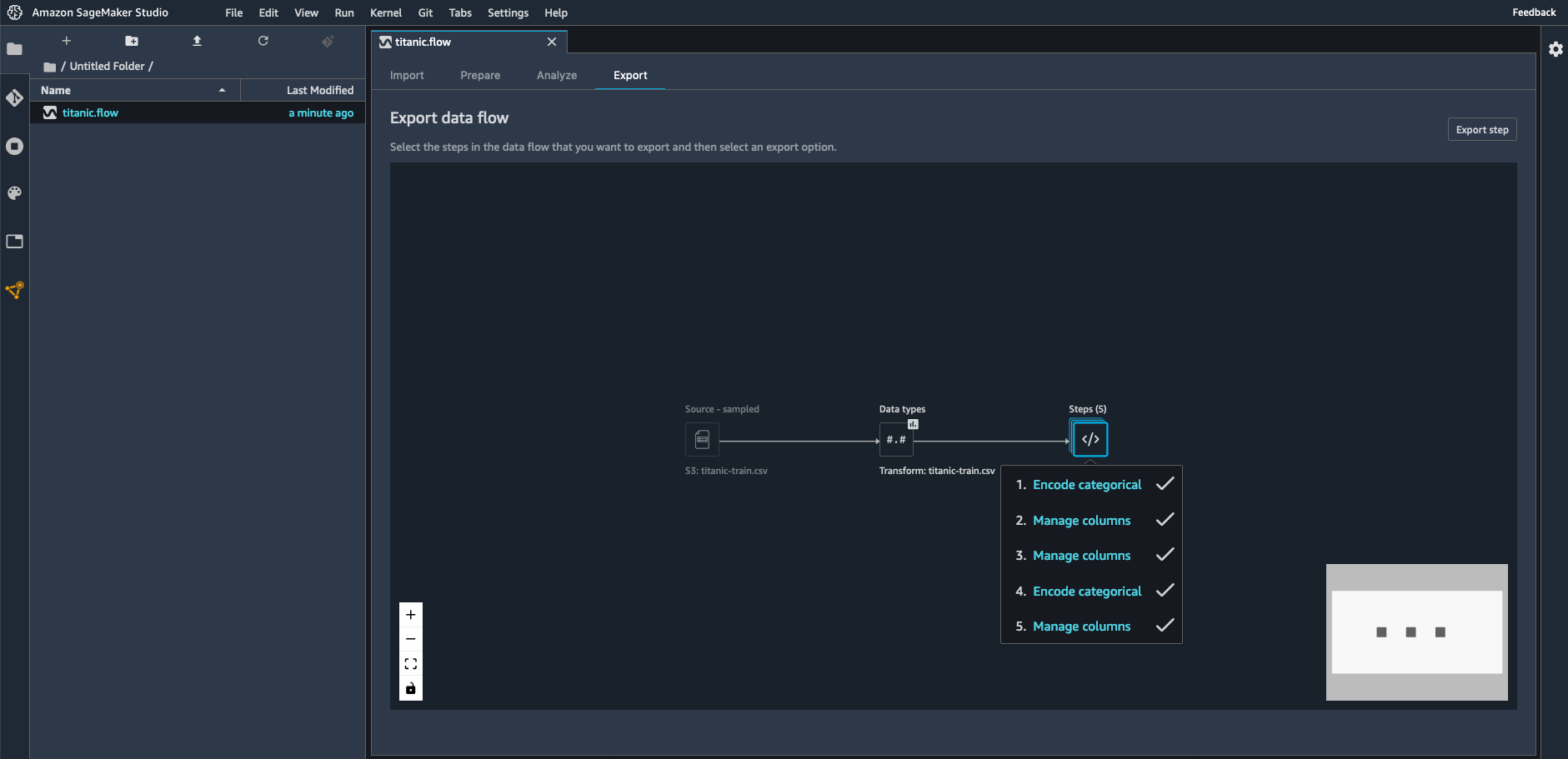
Then, moving to the “Export” view, I select all the transforms I’ve created so far, in order to add them to my ML project.

SageMaker screenshot

Here, I select “Python Code” to generate a Python script. Other options are available for Amazon SageMaker Processing, Amazon SageMaker Pipelines, and Amazon SageMaker Feature Store.

SageMaker screenshot

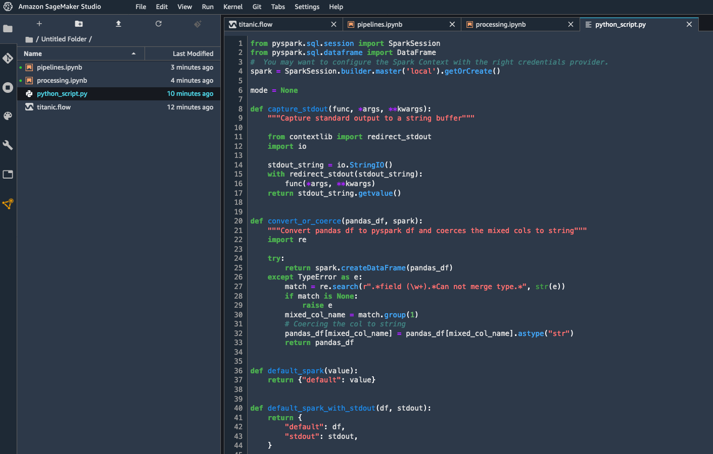
A few seconds later, the script is available. I could add it as is to my ML project, and rest assured that my data preparation steps would be consistent with the interactive transforms that I’ve created above.

SageMaker screenshot

Getting Started
As you can see, Amazon SageMaker Data Wrangler makes it really easy to work interactively on data preparation steps, before transforming them into code that can be used immediately for experimentation and production.

You can start using this capability today in all regions where SageMaker Studio is available.

Give it a try, and let us know what you think. We’re always looking forward to your feedback, either through your usual AWS support contacts, or on the AWS Forum for SageMaker.

– Julien

Special thanks to my colleague Peter Liu for his precious help during early testing.

New – Store, Discover, and Share Machine Learning Features with Amazon SageMaker Feature Store

Post Syndicated from Julien Simon original https://aws.amazon.com/blogs/aws/new-store-discover-and-share-machine-learning-features-with-amazon-sagemaker-feature-store/

Today, I’m extremely happy to announce Amazon SageMaker Feature Store, a new capability of Amazon SageMaker that makes it easy for data scientists and machine learning engineers to securely store, discover and share curated data used in training and prediction workflows.

For all the importance of selecting the right algorithm to train machine learning (ML) models, experienced practitioners know how crucial it is to feed it with high-quality data. Cleaning data is a good first step, and ML workflows routinely include steps to fill missing values, remove outliers, and so on. Then, they often move on to transforming data, using a mix of common and arcane techniques known as “feature engineering.”

Simply put, the purpose of feature engineering is to transform your data and to increase its expressiveness so that the algorithm may learn better. For instance, many columnar datasets include strings, such as street addresses. To most ML algorithms, strings are meaningless, and they need to be encoded in a numerical representation. Thus, you could replace street addresses with GPS coordinates, a much more expressive way to learn the concept of location. In other words, if data is the new oil, then feature engineering is the refining process that turns it into high-octane jet fuel that helps models get to stratospheric accuracy.

Indeed, ML practitioners spend a lot of time crafting feature engineering code, applying it to their initial datasets, training models on the engineered datasets, and evaluating model accuracy. Given the experimental nature of this work, even the smallest project will lead to multiple iterations. The same feature engineering code is often run again and again, wasting time and compute resources on repeating the same operations. In large organizations, this can cause an even greater loss of productivity, as different teams often run identical jobs, or even write duplicate feature engineering code because they have no knowledge of prior work.

There’s another hard problem that ML teams have to solve. As models are trained on engineered datasets, it’s imperative to apply the same transformations to data sent for prediction. This often means rewriting feature engineering code, sometimes in a different language, integrating it in your prediction workflow, and running it at prediction time. This whole process is not only time-consuming, it can also introduce inconsistencies, as even the tiniest variation in a data transform can have a large impact on predictions.

In order to solve these problems, ML teams sometimes build a feature store, a central repository where they can keep and retrieve engineered data used in their training and predictions jobs. As useful as feature stores are, building and managing your own involves a lot of engineering, infrastructure, and operational effort that takes valuable time away from actual ML work. Customers asked us for a better solution, and we got to work.

Introducing Amazon SageMaker Feature Store
Amazon SageMaker Feature Store is a fully managed centralized repository for your ML features, making it easy to securely store and retrieve features without having to manage any infrastructure. It’s part of Amazon SageMaker, our fully managed service for ML, and supports all algorithms. It’s also integrated with Amazon SageMaker Studio, our web-based development environment for ML.

Features stored in SageMaker Feature Store are organized in groups, and tagged with metadata. Thanks to this, you can quickly discover which features are available, and whether they’re suitable for your models. Multiple teams can also easily share and re-use features, reducing the cost of development and accelerating innovation.

Once stored, features can be retrieved and used in your SageMaker workflows: model training, batch transform, and real-time prediction with low latency. Not only do you avoid duplicating work, you also build consistent workflows that use the same consistent features stored in the offline and online stores.

The Climate Corporation (Climate) is a subsidiary of Bayer, and the industry leader in bringing digital innovation to farmers. Says Daniel McCaffrey, Vice President, Data and Analytics, Climate: “At Climate, we believe in providing the world’s farmers with accurate information to make data driven decisions and maximize their return on every acre. To achieve this, we have invested in technologies such as machine learning tools to build models using measurable entities known as features, such as yield for a grower’s field. With Amazon SageMaker Feature Store, we can accelerate the development of ML models with a central feature store to access and reuse features across multiple teams easily. SageMaker Feature Store makes it easy to access features in real-time using the online store, or run features on a schedule using the offline store for different use cases, and we can develop ML models faster.”

Care.com, the world’s leading platform for finding and managing high-quality family care, is also using Amazon SageMaker Feature Store. This is what Clemens Tummeltshammer, Data Science Manager, Care.com, told us: “A strong care industry where supply matches demand is essential for economic growth from the individual family up to the nation’s GDP. We’re excited about Amazon SageMaker Feature Store and Amazon SageMaker Pipelines , as we believe they will help us scale better across our data science and development teams, by using a consistent set of curated data that we can use to build scalable end-to-end machine learning model pipelines from data preparation to deployment. With the newly announced capabilities of Amazon SageMaker, we can accelerate development and deployment of our ML models for different applications, helping our customers make better informed decisions through faster real-time recommendations.”

Now, let’s see how you can get started.

Storing and Retrieving Features with Amazon SageMaker Feature Store
Once you’ve run your feature engineering code on your data, you can organize and store your engineered features in SageMaker Feature Store, by grouping them in feature groups. A feature group is a collection of records, similar to rows in a table. Each record has a unique identifier, and holds the engineered feature values for one of the data instances in your original data source. Optionally, you can choose to encrypt the data at rest using your own AWS Key Management Service (KMS) key that is unique for each feature group.

How you define feature groups is up to you. For example, you could create one per data source (CSV files, database tables, and so on), and use a convenient unique column as the record identifier (primary key, customer id, transaction id, and so on).

Once you’ve got your groups figured out, you should repeat the following steps for each group:

  1. Create feature definitions, with the name and the type of each feature in a record (Fractional, Integral, or String).
  2. Create each feature group with the create_feature_group() API:
    sm_feature_store.create_feature_group(
         # The name of the feature group
         FeatureGroupName=my_feature_group_name,
         # The name of the column acting as the record identifier
         RecordIdentifierName=record_identifier_name,
         # The name of the column action as the feature timestamp
         EventTimeFeatureName = event_time_feature_name,
         # A list of feature names and types
         FeatureDefinitions=my_feature_definitions,
         # The S3 location for the offline feature store
         OnlineStoreConfig=online_store_config,
         # Optionally, enable the online feature store
         OfflineStoreConfig=offline_store_config,
         # An IAM role
         RoleArn=role
    )
  3. In each feature group, store records containing a collection of feature name/feature value pairs, using the put_record() API:
    sm_feature_store.put_record(
       FeatureGroupName=feature_group_name,
       Record=record,
       EventTime=event_time
    )

    For faster ingestion, you could create multiple threads and parallelize this operation.

At this point, features will be available in Amazon SageMaker Feature Store. Thanks to the offline store, you can use services such as Amazon Athena, AWS Glue, or Amazon EMR to build datasets for training: fetch the corresponding JSON objects in S3, select the features that you need, and save them in S3 in the format expected by your ML algorithm. From then on, it’s SageMaker business as usual!

In addition, you can use the get_record() API to access individual records stored in the online store, passing the group name and the unique identifier of the record you want to access, like so:

record = sm_feature_store.get_record(
    FeatureGroupName=my_feature_group_name,
    RecordIdentifierValue={"IntegralValue": 5962}
)

Amazon SageMaker Feature Store is designed for fast and efficient access for real time inference, with a P95 latency lower than 10ms for a 15-kilobyte payload. This makes it possible to query for engineered features at prediction time, and to replace raw features sent by the upstream application with the exact same features used to train the model. Feature inconsistencies are eliminated by design, letting you focus on building the best models instead of chasing bugs.

Finally, as SageMaker Feature Store includes feature creation timestamps, you can retrieve the state of your features at a particular point in time.

As Amazon SageMaker Feature Store is integrated with SageMaker Studio, I can see my two features groups there.

SageMaker screenshot

Right-clicking on “Open feature group detail”, I open the identity feature group.

SageMaker screenshot

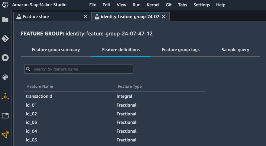
I can see feature definitions.

SageMaker screenshot

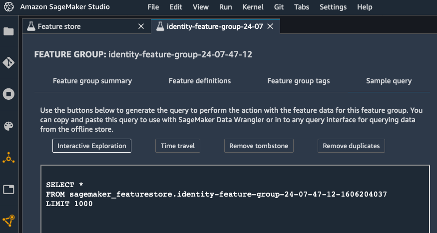
Finally, I can generate queries for the offline store, which I could add to a Amazon SageMaker Data Wrangler workflow to load features prior to training.

SageMaker screenshot

How to Get Started with Amazon SageMaker Feature Store
As you can see, SageMaker Feature Store makes it easy to store, retrieve, and share features required by your training and prediction workflows.

SageMaker Feature Store is available in all regions where SageMaker is available. Pricing is based on feature reads and writes, and on the total amount of data stored.

Here are sample notebooks that will help you get started right away. Give them a try, and let us know what you think. We’re always looking forward to your feedback, either through your usual AWS support contacts, or on the AWS Forum for SageMaker.

– Julien

Amazon SageMaker Edge Manager Simplifies Operating Machine Learning Models on Edge Devices

Post Syndicated from Julien Simon original https://aws.amazon.com/blogs/aws/amazon-sagemaker-edge-manager-simplifies-operating-machine-learning-models-on-edge-devices/

Today, I’m extremely happy to announce Amazon SageMaker Edge Manager, a new capability of Amazon SageMaker that makes it easier to optimize, secure, monitor, and maintain machine learning models on a fleet of edge devices.

Edge computing is certainly one of the most exciting developments in information technology. Indeed, thanks to continued advances in compute, storage, networking, and battery technology, organizations routinely deploy large numbers of embedded devices anywhere on the planet for a wide range of industry applications: manufacturing, energy, agriculture, healthcare, and more. Ranging from simple sensors to large industrial machines, the devices have a common purpose: capture data, analyze it, and act on it, for example send an alert if an unwanted condition is detected.

As machine learning (ML) demonstrated its ability to solve a wide range of business problems, customers tried to apply it to edge applications, training models in the cloud and deploying them at the edge in an effort to extract deeper insights from local data. However, given the remote and constrained nature of edge devices, deploying and managing models at the edge is often quite difficult.

For example, a complex model can be too large to fit, forcing customers to settle for a smaller and less accurate model. Also, predicting with several models on the same device (say, to detect different types of anomalies) may require additional code to load and unload models on demand, in order to conserve hardware resources. Finally, monitoring prediction quality is a major concern, as the real world will always be more complex and unpredictable than any training set can anticipate.

Customers asked us to help them solve these challenges, and we got to work.

Announcing Amazon SageMaker Edge Manager
Amazon SageMaker Edge Manager makes it easy for ML edge developers to use the same familiar tools in the cloud or on edge devices. It reduces the time and effort required to get models to production, while continuously monitoring and improving model quality across your device fleet.

Starting from a model that you trained or imported in Amazon SageMaker, SageMaker Edge Manager first optimizes it for your hardware platform using Amazon SageMaker Neo. Launched two years ago, Neo converts models into an efficient common format which is executed on the device by a low footprint runtime. Neo currently supports devices based on chips manufactured by Ambarella, ARM, Intel, NVIDIA, NXP, Qualcomm, TI, and Xilinx.

Then, SageMaker Edge Manager packages the model, and stores it in Amazon Simple Storage Service (S3), where it can be deployed to your devices. In fact, you can deploy multiple models, loading and predicting with a runtime optimized for your hardware of choice.

On-device models are managed by the SageMaker Edge Manager Manager Agent, which communicates with the AWS Cloud for model deployment, and with your application for model management. Indeed, you can integrate this agent with your application, so that it may automatically load and unload models according to your prediction requests. This enables a variety of scenarios, such as freeing all resources for a large model whenever needed, or working with a collection of smaller models that cohabit in memory.

Lenovo, the #1 global PC maker, recently incorporated Amazon SageMaker into its latest predictive maintenance offering. Igor Bergman, Lenovo Vice President, Cloud & Software of PCs and Smart Devices, told us: “At Lenovo, we’re more than a hardware provider and are committed to being a trusted partner in transforming customers’ device experience and delivering on their business goals. Lenovo Device Intelligence is a great example of how we’re doing this with the power of machine learning, enhanced by Amazon SageMaker. With Lenovo Device Intelligence, IT administrators can proactively diagnose PC issues and help predict potential system failures before they occur, helping to decrease downtime and increase employee productivity. By incorporating Amazon SageMaker Neo, we’ve already seen a substantial improvement in the execution of our on-device predictive models – an encouraging sign for the new Amazon SageMaker Edge Manager that will be added in the coming weeks. SageMaker Edge Manager will help eliminate the manual effort required to optimize, monitor, and continuously improve the models after deployment. With it, we expect our models will run faster and consume less memory than with other comparable machine learning platforms. As we extend AI to new applications across the Lenovo services portfolio, we will continue to require a high-performance pipeline that is flexible and scalable both in the cloud and on millions of edge devices. That’s why we selected the Amazon SageMaker platform. With its rich edge-to-cloud and CI/CD workflow capabilities, we can effectively bring our machine learning models to any device workflow for much higher productivity.”

Getting Started
As you can see, SageMaker Edge Manager makes it easier to work with ML models deployed on edge devices. It’s available today in the US East (N. Virginia), US West (Oregon), US East (Ohio), Europe (Ireland), Europe (Frankfurt), and Asia Pacific (Tokyo) regions.

Sample notebooks are available to get you started right away. Give them a try, and let us know what you think.

We’re always looking forward to your feedback, either through your usual AWS support contacts, or on the AWS Forum for SageMaker.

– Julien

New – Amazon SageMaker Clarify Detects Bias and Increases the Transparency of Machine Learning Models

Post Syndicated from Julien Simon original https://aws.amazon.com/blogs/aws/new-amazon-sagemaker-clarify-detects-bias-and-increases-the-transparency-of-machine-learning-models/

Today, I’m extremely happy to announce Amazon SageMaker Clarify, a new capability of Amazon SageMaker that helps customers detect bias in machine learning (ML) models, and increase transparency by helping explain model behavior to stakeholders and customers.

As ML models are built by training algorithms that learn statistical patterns present in datasets, several questions immediately come to mind. First, can we ever hope to explain why our ML model comes up with a particular prediction? Second, what if our dataset doesn’t faithfully describe the real-life problem we were trying to model? Could we even detect such issues? Would they introduce some sort of bias in imperceptible ways? As we will see, these are not speculative questions at all. They are very real, and their implications can be far-reaching.

Let’s start with the bias problem. Imagine that you’re working on a model detecting fraudulent credit card transactions. Fortunately, the huge majority of transactions are legitimate, and they make up 99.9% of your dataset, meaning that you only have 0.1% fraudulent transactions, say 100 out of 100,000. Training a binary classification model (legitimate vs. fraudulent), there’s a strong chance that it would be strongly influenced or biased by the majority group. In fact, a trivial model could simply decide that transactions are always legitimate: as useless as this model would be, it would still be right 99.9% of the time! This simple example shows how careful we have to be about the statistical properties of our data, and about the metrics that we use to measure model accuracy.

There are many variants of this under-representation problem. As the number of classes, features, and unique feature values increase, your dataset may only contain a tiny number of training instances for certain groups. In fact, some of these groups may correspond to various socially sensitive features such as gender, age range, or nationality. Under-representation for such groups could result in a disproportionate impact on their predicted outcomes.

Unfortunately, even with the best of intentions, bias issues may exist in datasets and be introduced into models with business, ethical, and regulatory consequences. It is thus important for model administrators to be aware of potential sources of bias in production systems.

Now, let’s discuss the explainability problem. For simple and well-understood algorithms like linear regression or tree-based algorithms, it’s reasonably easy to crack the model open, inspect the parameters that it learned during training, and figure out which features it predominantly uses. You can then decide whether this process is consistent with your business practices, basically saying: “yes, this is how a human expert would have done it.”

However, as models become more and more complex (I’m staring at you, deep learning), this kind of analysis becomes impossible. Just like the prehistoric tribes in Stanley Kubrick’s “2001: A Space Odyssey,” we’re often left staring at an impenetrable monolith and wondering what it all means. Many companies and organizations may need ML models to be explainable before they can be used in production. In addition, some regulations may require explainability when ML models are used as part of consequential decision making, and closing the loop, explainability can also help detect bias.

Thus, our customers asked us for help on detecting bias in their datasets and their models, and on understanding how their models make predictions. We got to work, and came up with SageMaker Clarify.

Introducing Amazon SageMaker Clarify
SageMaker Clarify is a new set of capabilities for Amazon SageMaker, our fully managed ML service. It’s integrated with SageMaker Studio, our web-based integrated development environment for ML, as well as with other SageMaker capabilities like Amazon SageMaker Data Wrangler, Amazon SageMaker Experiments, and Amazon SageMaker Model Monitor.

Thanks to SageMaker Clarify, data scientists are able to:

  • Detect bias in datasets prior to training, and in models after training.
  • Measure bias using a variety of statistical metrics.
  • Explain how feature values contribute to the predicted outcome, both for the model overall and for individual predictions.
  • Detect bias drift and feature importance drift over time, thanks to the integration with Amazon SageMaker Model Monitor.

Let’s look at each of these capabilities.

Detecting dataset bias: This is an important first step. Indeed, a heavily biased dataset may well be unsuitable for training. Knowing this early on certainly saves you time, money, and frustration! Looking at bias metrics computed by SageMaker Clarify on your dataset, you can then add your own bias reduction techniques to your data processing pipeline. Once the dataset has been revised and processed, you can measure bias again, and check if it has actually decreased.

Detecting model bias: After you’ve trained your model, you can run a SageMaker Clarify bias analysis, which includes automatic deployment to a temporary endpoint, and computation of bias metrics using your model and dataset. By computing these metrics, you can figure out if your trained model has similar predictive behavior across groups.

Measuring bias: SageMaker Clarify lets you pick from many different bias metrics. I’ll just give you a few examples here.

  • Difference in positive proportions in labels (DPL): Are labels in the dataset correlated or not with specific sensitive feature values? For example, do people living in a certain city have a better chance of getting a positive answer?
  • Difference in positive proportions in predicted labels (DPPL): Do we overpredict positive labels for a certain group?
  • Accuracy difference (AD): Are the predictions by the model more accurate for one group than the other?
  • Counterfactuals – Fliptest (FT): Suppose we look at each member of one group, and compare with similar members from the other group. Do they get different model predictions?

Explaining predictions – to explain how your model predicts, SageMaker Clarify supports a popular technique called SHapley Additive exPlanations (SHAP). Originating in game theory, SHAP analyzes for each data instance the individual contribution of feature values to the predicted output, and represents them as a positive or negative value. For example, predicting with a credit application model, you could see that Alice’s application is approved with a score of 87.5%, that her employment status (+27.2%) and her credit score (+32.4%) are the strongest contributors to this score, and that her income level has a slight negative impact (-5%). Such insights are crucial in building trust that the model is working as expected, and in explaining to customers and regulators why it comes up with a particular prediction. Further analysis of the SHAP values for your complete dataset can also help identify the relative importance of features and feature values, potentially leading to the discovery of prediction issues and biases.

As you can see, SageMaker Clarify has some pretty powerful features for bias detection and explainability. Fortunately, it also makes them very easy to use. First, you should upload a clean and pre-processed copy of your tabular dataset (CSV or JSON) to Amazon Simple Storage Service (S3). Then, using a built-in container, you just launch an Amazon SageMaker Processing job on your dataset, passing a short configuration file defining the name of the target attribute, the name and values of the sensitive columns to analyze for bias, and the bias metrics that you want to compute. As you would expect, this job runs on fully managed infrastructure. For post-training analysis, a temporary endpoint is also automatically created and deleted by the job. Once the job is complete, results are available in S3 and in SageMaker Studio, and include an auto-generated report that summarizes the results.

Now, I’d like to show you how to get started with SageMaker Clarify.

Exploring Datasets and Models with Amazon SageMaker Clarify
The German Credit Data dataset contains 1,000 labeled credit applications, which I’ve used to train a binary classification model with XGBoost. Each data instance has 20 features, such as credit purpose, credit amount, housing status, employment history, and more. Categorical features have been encoded with Axx values. For example, here’s how the credit history feature is encoded: A30 means ‘no credits taken’, A31 means ‘all credits at this bank paid back duly’, and so on.

In particular, the dataset includes a feature telling us if a customer is a foreign worker. In fact, a quick look at the dataset hints at a large imbalance in favor of foreign workers. Could bias be hiding there? What about the model? Did XGBoost increase or decrease the bias? Which features contribute most to the predicted output? Let’s find out.

After training the model, my next step is to run a SageMaker Clarify bias analysis job on the dataset, using a built-in container image that will compute bias metrics. The job inputs are the dataset, and a JSON configuration file that defines:

  • The name of the target attribute (Class1Good2Bad), and the value for the positive answer (1).
  • The sensitive features to analyze (called “facets”), and their value. Here, we want to focus on instances where ForeignWorker is set to 0, as they seem to be under-represented in the dataset.
  • The bias metrics that the job should compute. As I already have a model, I pass its name so that post-training metrics can be computed on a temporary endpoint.

Here’s the relevant snippet in the configuration file:

"label": "Class1Good2Bad",
"label_values_or_threshold": [1],
"facet": [
        {
         "name_or_index" : "ForeignWorker",
         "value_or_threshold": [0]
        }
    ],
. . .
"methods": {
    "pre_training_bias": {"methods": "all"}
    "post_training_bias": {"methods": "all"}
},
"predictor": {
        "model_name": "xgboost-german-model",
        "instance_type": "ml.m5.xlarge",
        "initial_instance_count": 1
    }

Then, I configure the job inputs (the dataset and the configuration file) and output (the report), passing all appropriate paths in S3:

config_input = ProcessingInput(
                    input_name="analysis_config",
                    source=analysis_config_s3_path,
                    destination="/opt/ml/processing/input/config")
data_input = ProcessingInput(
                    input_name="dataset",
                    source=train_data_s3_path,
                    destination="/opt/ml/processing/input/data")
result_output = ProcessingOutput(
                    source="/opt/ml/processing/output",
                    destination=analysis_result_s3_path,
                    output_name="analysis_result")

Finally, I run the processing job.

from sagemaker.processing import Processor, ProcessingInput, ProcessingJob, ProcessingOutput
analyzer_image_uri = f'678264136642.dkr.ecr.us-east-2.amazonaws.com/sagemaker-xai-analyzer:latest'
analyzer = Processor(base_job_name='analyzer',
                     image_uri=analyzer_image_uri,
                     role=sagemaker.get_execution_role(),
                     instance_count=1,
                     instance_type='ml.c5.xlarge')
analyzer.run(inputs=[ data_input, config_input], outputs=[result_output])

Once the processing job is complete, I can retrieve the report. Let’s look at bias metrics.

Detecting Bias with Amazon SageMaker Clarify
Here are some of the pre-training bias metrics:

"ForeignWorker": [
    {
     "value_or_threshold": "0",
     "metrics": [
      {
       "name": "CI",
       "description": "Class Imbalance (CI)",
       "value": 0.9225
      },
      {
       "name": "DPL",
       "description": "Difference in Positive Proportions in Labels (DPL)",
       "value": -0.21401904442300435
      },
. . . 

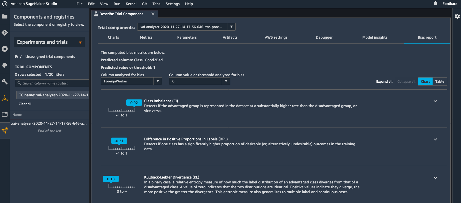
The class imbalance metric confirms our visual impression. The dataset has about 92% more foreign workers than it has domestic workers to assess. Whether this imbalance is responsible or not, we can also see that the difference in positive proportion for domestic workers is quite negative. In other words, there’s a smaller proportion of domestic workers with positive labels. This statistical pattern could be picked up by an ML algorithm, leading to a larger proportion of domestic workers getting negative answers. Figuring out whether this is actually legitimate or not would require further analysis, and in any case, it’s great that SageMaker Clarify warned us about this potential issue.

As I provided a trained model, post-training metrics are also available. Comparing the DPPL and the DPL, I can see that XGBoost has slightly reduced bias on positive proportions (-18.8% vs -21.4%). We also see that DAR is negative, indicating that the model achieves higher precision for domestic workers compared to foreign workers.

"ForeignWorker": [
    {
     "value_or_threshold": "0",
     "metrics": [
      {
       "name": "DPPL",
       "description": "\"Difference in Positive Proportions in Predicted Labels (DPPL)\")",
       "value": -0.18801124208230213
      },
      {
       "name": "DAR",
       "description": "Difference in Acceptance Rates (DAR)",
       "value": -0.050909090909090904
      },
      {
       "name": "DRR",
       "description": "Difference in Rejection Rates (DRR)",
       "value": 0.0365296803652968
      },
. . .

As SageMaker Clarify is integrated with SageMaker Studio, I can visualize bias metrics there. All I have to do is find the processing job in the list of trials, right-click “Open in trial details”, and select the “Bias report” view.

SageMaker screenshot

Finally, deciding whether high value of a certain bias metric is problematic involves domain-specific considerations. This needs to be guided by ethical, social, regulatory, and business considerations. Similarly, interventions for removing bias may often need a careful analysis of the entire ML lifecycle, from problem formulation to feedback loops in deployment.

Now, let’s see how SageMaker Clarify helps us understand what features the models base their predictions on.

Explaining Predictions with Amazon SageMaker Clarify
The report includes global SHAP values, showing the relative importance of all the features in the dataset. On the feature importance graph available in SageMaker Studio, I see that the three most important features are credit duration, not having a checking account (A14), and the loan amount. All things being equal, the bank probably sees you as a safer customer if you’re borrowing a small amount over a short period of time, and without the possibility to write checks!

SageMaker screenshot

In S3, I can also find a CSV file with SHAP values for individual data instances, giving me a complete picture of feature and feature value importance.

Getting Started
As you can see, SageMaker Clarify is a powerful tool to detect bias and to understand how your model works. You can start using it today in all regions where Amazon SageMaker is available, at no additional cost.

Sample notebooks are available to get you started quickly. Give them a try, and let us know what you think. We’re always looking forward to your feedback, either through your usual AWS support contacts, or on the AWS Forum for SageMaker.

– Julien

Special thanks to my colleagues Sanjiv Das, Michele Donini, Jason Gelman, Krishnaram Kenthapadi, Pinar Yilmaz, and Bilal Zafar for their precious help.

Dataset credits: Dua, D. and Graff, C. (2019). UCI Machine Learning Repository. Irvine, CA: University of California, School of Information and Computer Science.

In the Works – AWS Region in Melbourne, Australia

Post Syndicated from Jeff Barr original https://aws.amazon.com/blogs/aws/in-the-works-aws-region-in-melbourne-australia/

We launched new AWS Regions in Italy and South Africa in 2020, and are working on regions in Indonesia, Japan, Spain, India, and Switzerland.

Melbourne, Australia in 2020
Today I am happy to announce that the Asia Pacific (Melbourne) region is in the works, and will open in the second half of 2022 with three Availability Zones. In addition to the Asia Pacific (Sydney) Region, there are already seven Amazon CloudFront Edge locations in Australia, backed by a Regional Edge cache in Sydney.

This will be our second region in Australia, and our ninth in Asia Pacific, joining the existing region in Australia along with those in China, India, Japan, Korea, and Singapore. There are 77 Availability Zones within 24 AWS Regions in operation today, with 18 more Availability Zones and six more Regions (including this one) underway.

As part of our commitment to the Climate Pledge, Amazon is on a path to powering our operations with 100% renewable energy by 2025 as part of our goal to reach net zero carbon by 2040. To this end, we have invested in two renewable energy projects in Australia with a combined 165 MW capacity and the ability to generate 392,000 MWh annually.

The new region will give you (and hundreds of thousand of other active AWS customers in Australia) additional architectural options including the ability to store backup data in geographically separated locations within Australia.

AWS in Australia
I have made several trips to Australia on behalf of AWS over the last 4 or 5 years and I always enjoy meeting our customers while I am there.

Our Australian customers use AWS to accelerate innovation, increase agility, and to drive cost savings. Here are a few examples:

Commonwealth Bank of Australia (CBA) – As Australia’s leading provider of personal, business, and institutional banking services, CBA counts on AWS to provide infrastructure that is safe, resilient, and secure. They are long-time advocates of cloud computing and have been using AWS since 2012.

Swinburne University – The university focuses on innovation, industry engagement, and social inclusion. They started using AWS in 2016 and have collaborated on innovations that support communities in Victoria. The Swinburne Data for Social Good Cloud Innovation Centre uses cloud technologies and intelligent data analytics to solve real-world problems.

XY Sense – Based in Melbourne, this startup is using smart sensors and ML-powered analytics to create technology-enabled workplaces. Their sensor platform takes advantage of multiple AWS services including IoT and serverless, and processes over 7 billion anonymous data points each month.

AWS Partner Network (APN) Partners in Australia are also doing some amazing work with AWS. Again, a few examples:

Versent – Also based in Melbourne, this partner comprises a group of specialist consultants and a product company by the name of Stax. Versent recently helped Land Services South Australia to modernize their full tech stack as part of a shift to AWS (ready the case study to learn more).

Deloitte Australia – As an AWS Strategic Global Premier Partner since 2015, Deloitte Australia works with business and public sector agencies, with a focus on delivery of advanced products and services. As part of their work, over 4,000 employees across Deloitte have participated in the Deloitte Cloud Guild and have strengthened their cloud computing skills as a result.

Investing in Developers
Several AWS programs are designed to help to create and upskill the next generation of developers and students so that they are ready to become part of the next generation of IT leadership. AWS re/Start prepares unemployed, underemployed, and transitioning individuals for a career in cloud computing. AWS Academy provides higher education institutions with a free, ready-to-teach cloud computing curriculum. AWS Educate gives students access to AWS services and content that are designed to help them build knowledge and skills in cloud computing.

Stay Tuned
As I noted earlier, the Asia Pacific (Melbourne) Region is scheduled to open in the second half of 2022. As always, we’ll announce the opening in a post on this blog, so stay tuned!

— Jeff;

re:Invent 2020 Liveblog: Machine Learning Keynote

Post Syndicated from AWS News Blog Team original https://aws.amazon.com/blogs/aws/reinvent-2020-liveblog-machine-learning-keynote/

Swami Sivasubramanian speaks on stage at AWS re:InventFollow along as AWS Chief Evangelist Jeff Barr and Developer Advocates Martin Beeby and Steve Roberts liveblog the first-ever Machine Learning Keynote. Swami Sivasubramanian, VP of Amazon ML/AI will share the latest developments and launches in AWS machine learning, as well as demos of new technology, and insights from customers.

Join us here from 7:45-10 AM (PST), Tuesday, Dec. 8, 2020! 


Using Amazon CloudWatch Lambda Insights to Improve Operational Visibility

Post Syndicated from Steve Roberts original https://aws.amazon.com/blogs/aws/using-amazon-cloudwatch-lambda-insights-to-improve-operational-visibility/

To balance costs, while at the same time ensuring the service levels needed to meet business requirements are met, some customers elect to continuously monitor and optimize their AWS Lambda functions. They collect and analyze metrics and logs to monitor performance, and to isolate errors for troubleshooting purposes. Additionally, they also seek to right-size function configurations by measuring function duration, CPU usage, and memory allocation. Using various tools and sources of data to do this can be time-consuming, and some even go so far as to build their own customized dashboards to surface and analyze this data.

We announced Amazon CloudWatch Lambda Insights as a public preview this past October for customers looking to gain deeper operational oversight and visibility into the behavior of their Lambda functions. Today, I’m pleased to announce that CloudWatch Lambda Insights is now generally available. CloudWatch Lambda Insights provides clearer and simpler operational visibility of your functions by automatically collating and summarizing Lambda performance metrics, errors, and logs in prebuilt dashboards, saving you from time-consuming, manual work.

Once enabled on your functions, CloudWatch Lambda Insights automatically starts collecting and summarizing performance metrics and logs, and, from a convenient dashboard, provides you with a one-click drill-down into metrics and errors for Lambda function requests, simplifying analysis and troubleshooting.

Exploring CloudWatch Lambda Insights
To get started, I need to enable Lambda Insights on my functions. In the Lambda console, I navigate to my list of functions, and then select the function I want to enable for Lambda Insights by clicking on its name. From the function’s configuration view I then scroll to the Monitoring tools panel, click Edit, enable Enhanced monitoring, and click Save. If you want to enable enhanced monitoring for many functions, you may find it more convenient to use AWS Command Line Interface (CLI), AWS Tools for PowerShell, or AWS CloudFormation approaches instead. Note that once enhanced monitoring has been enabled, it can take a few minutes before data begins to surface in CloudWatch.

Screenshot showing enabling of <span title="">Lambda Insights</span> In the Amazon CloudWatch Console, I start by selecting Performance monitoring beneath Lambda Insights in the navigation panel. This takes me to the Multi-function view. Metrics for all functions on which I have enabled Lambda Insights are graphed in the view. At the foot of the page there’s also a table listing the functions, summarizing some data in the graphs and adding Cold starts. The table gives me the ability to sort the data based on the metric I’m interested in.

Screenshot of metric graphs on the <span title="">Lambda Insights</span> Multi-function viewScreenshot of the <span title="">Lambda Insights</span> Multi-function view summary listAn interesting graph on this page, especially if you are trying to balance cost with performance, is Function Cost. This graph shows the direct cost of your functions in terms of megabyte milliseconds (MB-MS), which is how Lambda computes the financial charge of a function’s invocation. Hovering over the graph at a particular point in time shows more details.

Screenshot of function cost graphLet’s examine my ExpensiveFunction further. Moving to the summary list at the bottom of the page I click on the function name which takes me to the Single function view (from here I can switch to my other functions using the controls at the top of the page, without needing to return to the multiple function view). The graphs show me metrics for invocations and errors, duration, any throttling, and memory, CPU, and network usage on the selected function and to add to the detail available, the most recent 1000 invocations are also listed in a table which I can sort as needed.
Clicking View in the Trace column of a request in the invocations list takes me to the Service Lens trace view, showing where my function spent its time on that particular invocation request. I could use this to determine if changes to the business logic of the function might improve performance by reducing function duration, which will have a direct effect on cost. If I’m troubleshooting, I can view the Application or Performance logs for the function using the View logs button. Application logs are those that existed before Lambda Insights was enabled on the function, whereas Performance logs are those that Lambda Insights has collated across all my enabled functions. The log views enable me to run queries and in the case of the Performance logs I can run queries across all enabled functions in my account, for example to perform a top-N analysis to determine my most expensive functions, or see how one function compares to another.

Here’s how I can make use of Lambda Insights to check if I’m ‘moving the needle’ in the correct direction when attempting to right-size a function, by examining the effect of changes to memory allocation on function cost. The starting point for my ExpensiveFunction is 128MB. By moving from 128MB to 512MB, the data shows me that function cost, duration, and concurrency are all reduced – this is shown at (1) in the graphs. Moving from 512MB to 1024MB, (2), has no impact on function cost, but it further reduces duration by 50% and also affected the maximum concurrency. I ran two further experiments, first moving from 1024MB to 2048MB, (3), which resulted in a further reduction in duration but the function cost started to increase so the needle is starting to swing in the wrong direction. Finally, moving from 2048MB to 3008MB, (4), significantly increased the cost but had no effect on duration. With the aid of Lambda Insights I can infer that the sweet spot for this function (assuming latency is not a consideration) lies between 1024MB and 2048MB. All these experiments are shown in the graphs below (the concurrency graph lags slightly, as earlier invocations are finishing up as configuration changes are made).
Screenshot of function cost experiments

CloudWatch Lambda Insights gives simple and convenient operational oversight and visibility into the behavior of my AWS Lambda functions, and is available today in all regions where AWS Lambda is present.
Learn more about Amazon CloudWatch Lambda Insights in the documentation and get started today.

— Steve

New – SaaS Lens in AWS Well-Architected Tool

Post Syndicated from Danilo Poccia original https://aws.amazon.com/blogs/aws/new-saas-lens-in-aws-well-architected-tool/

To help you build secure, high-performing, resilient, and efficient solutions on AWS, in 2015 we publicly launched the AWS Well-Architected Framework. It started as a single whitepaper but has expanded to include domain-specific lenses, hands-on labs, and the AWS Well-Architected Tool (available at no cost in the AWS Management Console) that provides a mechanism for regularly evaluating your workloads, identifying high risk issues, and recording your improvements.

To offer more workload-specific advice, in 2017 we extended the framework with the concept of “lens” to go beyond a general perspective and enter specific technology domains. Now, to help accelerate building Software-as-a-Service (SaaS) solutions, the AWS SaaS Factory team has led an effort to build a new AWS Well-Architected SaaS Lens.

SaaS is a licensing and delivery model by which software is centrally managed and hosted by a provider and available to customers on a subscription basis. In this way, software providers can innovate rapidly, optimize their costs, and gain operational efficiencies. At the same time, customers benefit from simplified IT management, speed, and a pay-for-what-you-use business model.

The Well-Architected SaaS Lens adds questions to the tool that are tailored to SaaS workloads and intended to drive critical thinking for developing and operating SaaS workloads. Each question has a list of best practices, and each best practice has a list of improvement plans to help guide you in implementing them. AWS Solution Architects from the AWS SaaS Factory Program, having worked with thousands of software developers and AWS Partners, view these well-architected patterns as a key component of building and operating a SaaS architecture on AWS.

Using the SaaS Lens in the Well-Architected Tool
In the Well-Architected Tool console, I start by defining my workload. Today, I’m reviewing a pre-production environment of a SaaS application. It’s just a minimum viable product (MVP) version of what I want to build, with just enough features to be usable and get a first feedback.

Now, I can choose which lenses to apply. The AWS Well-Architected Framework is there by default. I select the SaaS Lens. This is adding a set of additional questions that help me understand how to design, deploy, and architect my SaaS workload following the framework best practices. Other lenses are available in the tool, for example the Serverless Lens described here.

Now, I start my review. Many questions in the SaaS Lens are focused on how you are managing a multi-tenant application. This is the first question for the Operational Excellence pillar. I can also add some notes to explain my answer better or take note of what I want to improve.

I don’t need to answer all questions to start improving my SaaS application. For example, this is the improvement plan based on my answer to the previous question. For each point here, I can click and get more information on how to implement that on AWS.

Moving to the Reliability pillar, I feel more confident because of the techniques I used to separate individual tenants of my SaaS application in their own “sandbox” environment.

As I expect, no risks are detected this time!

When I finish reviewing the SaaS Lens for my workload, I get an overview of the detected risks. Here, I can also save a milestone that I can use later to compare my status and estimate my improvements.

Just below that, I get a suggestion on what to focus on next. Again, I can click and get in-depth suggestion on how to mitigate the risk.

As often happens in IT services, this is an iterative process. The AWS Well-Architected Tool helps quantify the risks and gives me a path to follow to continuously improve my SaaS application.

Available Now
The SaaS Lens is available today in all regions where the AWS Well-Architected Tool is offered, as described in the AWS Regional Services List. It can be applied to existing workloads, or used for new workloads you define in the tool.

There are no costs in using the AWS Well-Architected Tool; you can use it to improve the application you are working on, or to get visibility into multiple workloads used by the department or area you are working with.

Learn more about the new SaaS Lens and get started today with the AWS Well-Architected Tool!

— Danilo

re:Invent 2020 Liveblog: Partner Keynote

Post Syndicated from AWS News Blog Team original https://aws.amazon.com/blogs/aws/reinvent-2020-liveblog-partner-keynote/

Join us Thursday, Dec. 3, from 7:45-9:30 a.m., for the AWS Partner Keynote with Doug Yeum, head of Worldwide Channels and Alliances; Sandy Carter, vice president, Global Public Sector Partners and Programs; and Dave McCann, vice president, AWS Migration, Marketplace, and Control Services. Developer Advocates Steve Roberts and Martin Beeby will be liveblogging all the announcements and discussion.

See you at 7:45 a.m. (PST) Thursday!

— Steve & — Martin


Amazon S3 Update – Strong Read-After-Write Consistency

Post Syndicated from Jeff Barr original https://aws.amazon.com/blogs/aws/amazon-s3-update-strong-read-after-write-consistency/

When we launched S3 back in 2006, I discussed its virtually unlimited capacity (“…easily store any number of blocks…”), the fact that it was designed to provide 99.99% availability, and that it offered durable storage, with data transparently stored in multiple locations. Since that launch, our customers have used S3 in an amazing diverse set of ways: backup and restore, data archiving, enterprise applications, web sites, big data, and (at last count) over 10,000 data lakes.

One of the more interesting (and sometimes a bit confusing) aspects of S3 and other large-scale distributed systems is commonly known as eventual consistency. In a nutshell, after a call to an S3 API function such as PUT that stores or modifies data, there’s a small time window where the data has been accepted and durably stored, but not yet visible to all GET or LIST requests. Here’s how I see it:

This aspect of S3 can become very challenging for big data workloads (many of which use Amazon EMR) and for data lakes, both of which require access to the most recent data immediately after a write. To help customers run big data workloads in the cloud, Amazon EMR built EMRFS Consistent View and open source Hadoop developers built S3Guard, which provided a layer of strong consistency for these applications.

S3 is Now Strongly Consistent
After that overly-long introduction, I am ready to share some good news!

Effective immediately, all S3 GET, PUT, and LIST operations, as well as operations that change object tags, ACLs, or metadata, are now strongly consistent. What you write is what you will read, and the results of a LIST will be an accurate reflection of what’s in the bucket. This applies to all existing and new S3 objects, works in all regions, and is available to you at no extra charge! There’s no impact on performance, you can update an object hundreds of times per second if you’d like, and there are no global dependencies.

This improvement is great for data lakes, but other types of applications will also benefit. Because S3 now has strong consistency, migration of on-premises workloads and storage to AWS should now be easier than ever before.

We’ve been working with the Amazon EMR team and developers in the open-source community to ensure that customers can take advantage of this update with their big data workloads. As a result of that you no longer need to use EMRFS Consistent View or S3Guard, further reducing the cost to run big data workloads in AWS.

A Word From Dropbox
Long-time AWS customer Dropbox recently migrated a 34 PB analytics data lake from on-premises Hadoop clusters to S3. Watch this video to learn more about strong consistency and how it has allowed Dropbox to simplify their data lake:

— Jeff;


AWS re:Invent: Top Announcements for 2020

Post Syndicated from AWS News Blog Team original https://aws.amazon.com/blogs/aws/aws-reinvent-announcements-2020/

Compute | Containers | Customer Engagement | Database | Machine Learning |

Below are the major launch and preview announcements happening at re:Invent 2020, organized by category. We’ll update this page daily over the course of the event, which takes place Nov. 30-Dec. 18. For a list of re:Invent launch posts by date, you can find the full list here.

Compute

New – Use Amazon EC2 Mac Instances to Build and Test macOS, iOS, ipadOS, tvOS, and watchOS Apps
Over the last couple of years, AWS users have told us that they want to be able to run macOS on Amazon Elastic Compute Cloud (EC2). We’ve asked a lot of questions to learn more about their needs, and today we introduce you to the new Mac instance!

re:Invent 2020 Pre-announcements for Tuesday, December 1
Here’s a sneak peek at some good things to come, including: AWS Outpost Servers, Amazon ECS Anywhere and Amazon EKS Anywhere.

Coming Soon – Amazon EC2 G4ad Instances Featuring AMD GPUs for Graphics Workloads
Customers with high performance graphic workloads, such as those in game streaming, animation, and video rendering, are always looking for higher performance at less cost. Today, we announce that new Amazon Elastic Compute Cloud (EC2) instances in the G4 instance family will be available soon to improve performance and reduce cost for graphics-intensive workloads.

New EC2 C6gn Instances – 100 Gbps Networking with AWS Graviton2 Processors
Today, we’re expanding our broad Arm-based Graviton2 portfolio with C6gn instances that deliver up to 100 Gbps network bandwidth, up to 38 Gbps Amazon Elastic Block Store (EBS) bandwidth, up to 40% higher packet processing performance, and up to 40% better price/performance versus comparable current generation x86-based network optimized instances.

EC2 Update – D3 / D3en Dense Storage Instances
We have launched several generations of EC2 instances with dense storage including the HS1 in 2012 and the D2 in 2015. Today we are launching the D3 and D3en instances. Like their predecessors, they give you access to massive amounts of low-cost on-instance HDD storage.

New – Amazon EC2 R5b Instances Provide 3x Higher EBS Performance
R5 instances are designed for memory-intensive applications such as high-performance databases, distributed web scale in-memory caches, in-memory databases, real time big data analytics, and other enterprise applications. Today, we announce the new R5b instance, which provides the best network-attached storage performance available on EC2.

New for AWS Lambda – 1ms Billing Granularity Adds Cost Savings
Since Lambda was launched in 2014, pricing has been based on the number of times code is triggered (requests) and the number of times code executes, rounded up to the nearest 100ms (duration). Starting today, we are rounding up duration to the nearest millisecond with no minimum execution time.

In the Works – 3 More AWS Local Zones in 2020, and 12 More in 2021
We launched the first AWS Local Zone in Los Angeles last December, and added a second one (also in Los Angeles) in August of 2020. With 3 more available today and 12 planned next year, we are choosing the target cities with the goal of allowing you to provide access with single-digit millisecond latency to the vast majority of users in the Continental United States.

New for AWS Lambda – Container Image Support
With Lambda, you upload your code and run it without thinking about servers. Many customers enjoy the way this works, but if you’ve invested in container tooling for your development workflows, it’s not easy to use the same approach to build applications using Lambda. To help you with that, you can now package and deploy Lambda functions as container images of up to 10 GB in size.

Containers

Amazon ECR Public: A New Public Container Registry
You have long been able to host private container images on AWS with Amazon Elastic Container Registry, and now with the release of Amazon Elastic Container Registry Public, you can host public ones too, enabling anyone (with or without an AWS account) to browse and pull your published containers.

Preview of AWS Proton – Automated Management for Container and Serverless Deployments
Maintaining hundreds – or sometimes thousands – of microservices with constantly changing infrastructure resources and configurations is a challenging task for even the most capable teams. AWS Proton enables infrastructure teams to define standard templates centrally and make them available for developers in their organization. This allows infrastructure teams to manage and update infrastructure without impacting developer productivity.

Customer Engagement

Amazon Connect – Now Smarter and More Integrated With Third-Party Tools
We launched Amazon Connect in 2017 and, since then, thousands of customers have created their own contact centers in the cloud. Amazon Connect makes it easy for non-technical customers to design interaction flows, manage agents, and track performance metrics. Today, we announce a new set of capabilities to make Amazon Connect smarter and more integrated with third-party tools.

Database

New – Amazon QuickSight Q Answers Natural-Language Questions About Business Data
Today, we are happy to announce the preview of Amazon QuickSight Q, a Natural Language Query (NLQ) feature powered by machine learning (ML). With Q, business users can now use QuickSight to ask questions about their data using everyday language and receive accurate answers in seconds.

Now in Preview – Larger and Faster io2 Block Express EBS Volumes with Higher Throughput
Earlier this year we launched io2 volumes with 100x higher durability and 10x more IOPS/GiB than the earlier io1 volumes. Today we are opening up a preview of io2 Block Express volumes that are designed to deliver even higher performance!

New – Amazon EBS gp3 Volume Lets You Provision Performance Apart From Capacity
When using general purpose SSD gp2 volumes with EBS, performance is associated with storage capacity. Today we announce the new gp3 volume that lets customers increase IOPS and throughput without having to provision additional block storage capacity, paying only for the resources they need.

Machine Learning

New- Amazon DevOps Guru Helps Identify Application Errors and Fixes
Today, we are announcing Amazon DevOps Guru, a fully managed operations service that makes it easy for developers and operators to improve application availability by automatically detecting operational issues and recommending fixes.

Amazon Lookout for Equipment Analyzes Historical Sensor Data to Help Detect Equipment Failure
Companies that operate industrial equipment are constantly working to improve operational efficiency and avoid unplanned downtime due to component failure. Amazon Lookout for Equipment is an API-based machine learning (ML) service that detects abnormal equipment behavior and helps companies monitor the health of their assets.

Amazon Lookout for Vision Simplifies Defect Detection for Manufacturing
Lookout for Vision is a new machine learning service that helps increase industrial product quality and reduce operational costs by automating visual inspection of product defects across production processes. Using Lookout for Vision, you can detect damages to manufactured parts, identify missing components or parts, and uncover underlying process-related issues in your manufacturing lines.

AWS Panorama Appliance – Bringing Computer Vision Applications to the Edge
Today we preview the AWS Panorama Appliance and its associated console. You can now develop a computer vision model using Amazon SageMaker and then deploy it to a Panorama Appliance that can then run the model on video feeds from multiple network and IP cameras.

Amazon Monitron is a Simple and Cost-Effective Service Enabling Predictive Maintenance
Monitron is an easy and cost-effective condition monitoring service that allows you to monitor the condition of equipment in your facilities, enabling the implementation of a predictive maintenance program.

In the Works – 3 More AWS Local Zones in 2020, and 12 More in 2021

Post Syndicated from Jeff Barr original https://aws.amazon.com/blogs/aws/in-the-works-more-aws-local-zones/

We launched the first AWS Local Zone in Los Angeles last December, and added a second one (also in Los Angeles) in August of 2020. In my original post, I quoted Andy Jassy’s statement that we would be giving consideration to adding Local Zones in more geographic areas.

Our customers are using the EC2 instances and other compute services in these zones to host artist workstations, local rendering, sports broadcasting, online gaming, financial transaction processing, machine learning inferencing, virtual reality, and augmented reality applications, among others. These applications benefit from the extremely low latency made possible by geographic proximity.

More Local Zones
I’m happy to be able to announce that we are opening three more Local Zones today and plan to open twelve more in 2021.

Local Zones in Boston, Houston, and Miami are now available in preview form and you can request access now. In 2021, we plan to open Local Zones in other key cities and metropolitan areas including New York City, Chicago, and Atlanta.

We are choosing the target cities with the goal of allowing you to provide access with single-digit millisecond latency to the vast majority of users in the Continental United States. You can deploy the parts of your application that are the most sensitive to latency in Local Zones, and deliver amazing performance to your users. In addition to the use cases that I mentioned above, I expect to see many more that have yet to be imagined or built.

Using Local Zones
I stepped through the process of using a Local Zone in my original post, and all that I said there still applies. Here’s what you need to do:

  1. Request access to the preview and await a reply.
  2. Create a new VPC subnet for the Local Zone.
  3. Launch EC2 instances, create EBS volumes, and deploy your application.

Things to Know
Here are a couple of things that you should know about the new and upcoming Local Zones:

Instance Types – The Local Zones will have a wide selection of EC2 instance types including C5, R5, T3, and G4 instances..

Purchasing Models – You can use compute capacity in Local Zones on an On-Demand basis and you can also purchase a Savings Plan in order to receive discounts. Some of the Local Zones also support the use of Spot Instances, .

AWS Services – Local Zones support Amazon Elastic Compute Cloud (EC2), Amazon Elastic Block Store (EBS), Amazon Elastic Kubernetes Service (EKS), and Amazon Virtual Private Cloud, with the door open for other services in the future. You can use services such as Auto Scaling, AWS CloudFormation, and Amazon CloudWatch in the parent region to launch, control, and monitor the AWS resources in a Local Zone.

Direct Connect – As I mentioned earlier, some of our customers are using AWS Direct Connect to establish private connections between Local Zones and their existing on-premises or colo IT infrastructure. We are working with our Direct Connect Partners to make Direct Connect available for the new zones and the specifics will vary on a zone-by-zone basis.

The AWS Local Zones Features page contains additional zone-by-zone information on all of the items listed above.

Learn More
Here are some resources to help you to learn more about Local Zones:

Blog Post – Low-Latency Computing with AWS Local Zones.

Sites – AWS Local Zones home page, AWS Local Zones FAQ.

— Jeff;

re:Invent 2020 – Preannouncements for Tuesday, December 1

Post Syndicated from Jeff Barr original https://aws.amazon.com/blogs/aws/reinvent-2020-preannouncements-for-tuesday-december-1/

Andy Jassy just gave you a hint about some upcoming AWS launches, and I’ll have more to say about them when they are ready. To tide you over until then, here’s a summary of what he pre-announced:

Smaller AWS Outpost Form Factors – We are introducing two new sizes of AWS Outposts, suitable for locations such as branch offices, factories, retail stores, health clinics, hospitals, and cell sites that are space-constrained and need access to low-latency compute capacity. The 1U (rack unit) Outposts server will be equipped with AWS Graviton 2 processors; the 2U Outposts server will be equipped with Intel® processors. Both sizes will be able to run EC2, ECS, and EKS workloads locally, all provisioned and managed by AWS (including automated patching and updates).

Amazon ECS Anywhere – You will soon be able to run Amazon Elastic Container Service (ECS) in your own data center, giving you the power to select and standardize on a single container orchestrator that runs both on-premises and in the cloud. You will have access to the same ECS APIs, and you will be able to manage all of your ECS resources with the same cluster management, workload scheduling, and monitoring tools and utilities. Amazon ECS Anywhere will also make it easy for you to containerize your existing on-premises workloads, run them locally, and then connect them to the AWS Cloud.

Amazon EKS Anywhere – You will also soon be able to run Amazon Elastic Kubernetes Service (EKS) in your own data center, making it easy for you to set up, upgrade, and operate Kubernetes clusters. The default configuration for each new cluster will include logging, monitoring, networking, and storage, all optimized for the environment that will host the cluster. You will be able to spin up clusters on demand, and you will be able to backup, recover, patch, and upgrade production clusters with minimal disruption.

Again, I’ll have more to say about these when they are ready, so stay tuned, and enjoy the rest of AWS re:Invent!

— Jeff;

Amazon Connect – Now Smarter and More Integrated With Third-Party Tools

Post Syndicated from Sébastien Stormacq original https://aws.amazon.com/blogs/aws/amazon-connect-smarter-and-more-integrated/

We launched Amazon Connect in 2017 and, since then, thousands of customers have created their own contact centers in the cloud. Amazon Connect makes it easy for non-technical customers to design interaction flows, manage agents, and track performance metrics.

For example, when I book a Best Western hotel room in Europe by phone, the call is managed by Amazon Connect. In the UK, the Post Office went from ideation to production rollout in just three weeks. In France, WebHelp, a global leader in Business Process Outsourcing, activated thousands of workstations and remote agents in just 72 hours.

Since I last blogged about Amazon Connect, the team has been continuously listening for your feedback and, today, I am happy to announce a new set of capabilities to make Amazon Connect smarter and more integrated with third-party tools.

We are using Machine Learning (ML) to make Amazon Connect smarter at analyzing conversations in real time, finding relevant information needed by contact center agents, and authenticating customers by the sound of their voice. The second set of capabilities makes Amazon Connect easier to integrate with third party tools or services to present unified customer profile information to contact center agents, and to make it easier to manage their tasks.

Let’s go into the details, one by one.

Contact Lens Real Time
Contact Lens for Amazon Connect is a set of machine learning (ML) capabilities allowing contact center supervisors to better understand the sentiment, trends, and compliance of customer conversations. It was first announced during re:Invent 2019 and available since July 2020. It allows to effectively train agents, replicate successful interactions, and to identify crucial company and product feedback.

Starting today, you can get real-time insights into customer experience during the live calls, such as a customer expressing dissatisfaction. Customer experience analytics and alerts for live calls are delivered in Amazon Connect’s real-time metrics dashboard. It makes it easy for supervisors to identify when to listen-in on a critical call, and to provide guidance to the agent via chat, or have the agent transfer the call to them for assistance.

You, as the contact center manager, can define rules using specific terms such as “not happy,” “poor quality product,” and “cancel my subscription.” Contact Lens uses natural language processing (NLP) to perform intelligent matching to automatically detect variations of the spoken words even when the example phrases are limited.

Create Rules for real time analytics

Contact Lens analyzes in-progress calls in real time to detect when the rule criteria for a customer experience issue is met, and immediately creates an alert next to the live call in the Amazon Connect dashboard to notify supervisors of the situation.

Real Time alert based on rules

With this launch, we are adding 13 language variants to post-call analytics, in addition to the 5 already supported :English (United States), English (Great Britain), English (Australia), English (India), and Spanish (United States).

The new language variants for post-call analytics are: English (Ireland), English (Scotland), English (Wales), Spanish (Spain), French (Canada), French (France), Portuguese (Portugal), Portuguese (Brazil), German (Germany), German (Switzerland), Italian (Italy), Arabic (Gulf), and Hindi (India).

Contact Lens for Amazon Connect real-time is available in 4 language variants: English (United States), English (Great Britain), English (Australia), and Spanish (United States). More language variants will be added at later stage.

For more details visit this launch page.

Amazon Connect Wisdom (Preview)
Wisdom provides built-in agent assistance capabilities in Amazon Connect, including machine learning (ML) powered search and real-time recommendations, to quickly enable agents with relevant information for resolving customer issues.

As an agent, I can type questions or phrases in the Wisdom search box, without guessing what keyword I should use. Wisdom understands what information I am searching for. It surfaces results in the agent’s preferred Amazon Connect application, the web-based one we do provide, or the ones you built.

Amazon Connect Wisdom search results

Wisdom comes with pre-built connectors to third-party knowledge repositories to provide most relevant results to agents. Wisdom includes connectors for Salesforce and ServiceNow during the preview, with more to come at launch.

Wisdom may use Contact Lens Real Time analytics to analyse the conversation in real-time. It detects the customer issue, finds related content in the connected repositories, and provides proactive recommendations to help the agent resolve it. For example, Wisdom can detect that a customer is talking about a problem with the handbag they bought last week, recommend an article that describes similar products defect, and provide instructions with a link to the order management application needed to initiate an exchange.

Wisdom is available in preview, you can signup today or visit the launch page.

Amazon Connect Voice ID (Preview)
Amazon Connect Voice ID provides real-time caller authentication which makes voice interactions in contact centers more secure and efficient.

To effectively recognise me as “Sébastien”, Voice ID must learn how I am talking. This is the enrolment phase. Then it compares the sound of my voice with the one enrolled earlier. This is the verification phase.

To meet with personal data protection laws, contact center agents capture my consent to use Voice ID.

During the enrolment phase, Voice ID listens to the call until it has captured 30 seconds of my voice. Then it creates my voiceprint, which uniquely authenticates me. A voiceprint is a mathematical representation that captures unique aspects of an individual’s voice such as speech rhythm, pitch, intonation, and loudness. I do not need to say or repeat any specific phrases to let Voice ID create my voiceprint. Voice ID provides an API that can be used to opt-out a customer.

When I call back in, Voice ID just needs 10 seconds of my voice to authenticate me. My voice can be captured as part of a typical interaction with the Interactive Voice Response (IVR) happening at the start of the call, or when I first start to talk with the agent. For example when I am answering questions, such as “what’s your first and last name?” and “what are you calling about?”, Voice ID uses this audio to generate my voiceprint again. It compares it with the one enrolled earlier. Voice ID then generates an authentication score depending on the confidence of the match. Contact center managers can use this score to create policies in Amazon Connect to let agents see a real-time result (“authenticated” or “not authenticated”) in their web-based application. Agents can then decide to proceed with the call or ask for additional authentication credentials.

Amazon Connect Voice ID is available in preview. You can signup today or visit this launch page.

Amazon Connect Customer Profiles
Customer Profiles is a unified profile for Amazon Connect that brings together customer information from disparate sources without having to build integrations or wrangle data.

Providing agents (or automatic IVR systems) with accurate and unified customer profile information at the right moment helps them to deliver better service to customers, and to resolve calls faster. Using Customer Profiles, agents must not navigate out of Amazon Connect, or switch between different applications to get the customer insights they need.

With just a few clicks, System Administrators can integrate customer profile data from applications like Salesforce, ServiceNow, Zendesk, and Marketo to build your own homegrown integration. Setting up connectors for Customer Profiles requires no programming or data integration expertise.

Once enabled, Customer Profiles automatically detects customer records from the applications. It matches and deduplicates them. This results in accurate and up-to-date profiles displayed to agents within their Connect web-based experience.

Amazon Connect Customer Profile

Learn more about Amazon Connect Customer Profile by visiting the launch page.

Amazon Connect Tasks
Amazon Connect Tasks makes it easy to automate, track, and manage contact center agent tasks. It provides a single place for contact center managers to prioritize, assign, and track customer service tasks across the disparate applications used by agents, so that they are focused on the highest priority work of any type.

Tasks can be sourced from third-party applications, such as a CRM solution, or to update a business-specific system. For example, you can programmatically create tasks for agents to follow-up on a customer case in a third party application like Salesforce, or complete an action item in a business-specific application, such as processing a claim in an insurance system. You can also automate tasks that dont require agent interaction, to ensure your agents spend more time focused on customers.

Using Amazon Connect tasks, agents no longer need to switch between applications to know what work should be completed, and with what priority. Agents can see all their assigned tasks right from the Amazon Connect contact control panel, the same web-based application they use to interact with customers over calls and chat. When a task is assigned, the agent receives a notification with the description of the task, and when required, links to any external applications needed to complete the action. Agents can also create tasks so that follow-up work is not forgotten, for example calling a customer back to provide a status update.

Amazon Connect Accept Tasks Amazon Connect View Task Create a task uisng Amazon Connect Tasks
Incoming Tasks Task Details Create a new Task

Amazon Connect Tasks provides pre-built connectors fo Salesforce and Zendesk. With just a few clicks, you can easily set up rules to automatically create tasks based on pre-defined conditions, as sown on the screenshot hereunder. It also provides an API to create tasks from any other application.

Amazon Connect Task Rules

Learn more about how to configure and to get started with Tasks by visiting the launch page.

Available Today
Three of these new capabilities are available today: Contact Lens Real Time, Customer Profiles, and Tasks. You must register to the preview program to test Wisdom and Voice ID.

Customer Profile and Tasks are available in all AWS Regions where Amazon Connect is available : US East (N. Virginia), US East (Ohio), US West (N. California), US West (Oregon), Asia Pacific (Sydney), Asia Pacific (Singapore), Asia Pacific (Tokyo), Europe (Frankfurt), and Europe (London). Contact Lens Real Time is available in US West (Oregon), US East (N. Virginia), and Asia Pacific (Sydney) at the moment. Wisdom is available in US East (N. Virginia) and US West (Oregon) during the preview, while Voice ID is available only in US West (Oregon) during the preview.

With Amazon Connect, you only pay for what you use. There are no required up-front payments, long-term commitments, or minimum monthly fees. The price metrics for these new capabilities are detailed on the Amazon Connect pricing page.

Should you need help adding Amazon Connect any of these capabilities to contact flows, please reach out to one of the dozens of Amazon Connect partners available worldwide.

— seb

New for AWS Lambda – Functions with Up to 10 GB of Memory and 6 vCPUs

Post Syndicated from Danilo Poccia original https://aws.amazon.com/blogs/aws/new-for-aws-lambda-functions-with-up-to-10-gb-of-memory-and-6-vcpus/

AWS Lambda runs your code on an highly available and scalable compute infrastructure so that you can focus on what you want to build. Do you want to get the advantages of Lambda for workloads that are memory or computationally intensive? Wait no more!

Starting today, you can allocate up to 10 GB of memory to a Lambda function. This is more than a 3x increase compared to previous limits. Lambda allocates CPU and other resources linearly in proportion to the amount of memory configured. That means you can now have access to up to 6 vCPUs in each execution environment. In this way, your multithreaded and multiprocess applications run faster. Since Lambda charges are proportional to memory configured and function duration (GB-seconds), the additional costs for using more memory may be offset by lower duration. I have more on this in the example below.

With more memory and CPU power, and support for the AVX2 instruction set, new use cases — such as machine learning applications; batch and extract, transform, load (ETL) jobs; modelling; genomics; gaming; high-performance computing (HPC); and media processing — become easier to implement and scale with Lambda functions.

Let’s see how this works in practice!

Lambda Function Performance as Memory Increases
When I first wrote about the capability of mounting a shared Amazon Elastic File System (EFS) for Lambda functions, one of the examples I used was a function doing machine learning inference to classify images of birds. The function is using PyTorch to run the inference, applying a pre-trained machine learning model.

Now, I can execute the same function in the updated Lambda execution environment. Let’s see how increasing memory affects the duration of the function. Here are the results of using memory configurations between 1 and 10 GB. To get these numbers, I ran 20 invocations for each memory configuration. Then, I computed the average duration, discarding function initializations. To avoid possible outliers, I also excluded from the average the top and bottom 10% of reported durations. Based on the results, I estimated the charges I would have for 1 million invocations with each configuration.

Graph showing Function Duration and Charges for 1M Invocations as Memory Increases

As you can see, the function is able to use the additional CPU power that comes with more memory, decreasing the duration of the invocations. What is interesting is the impact of increasing memory on my costs.

Lambda charges are related to memory and duration, so if I increase memory and this is reducing duration by the same proportion, the overall charges are about the same. For example, looking at the graph above, when I configure 5 GB of memory, I have the same costs as when I have 1 GB of memory (about $61 for one million invocations), but the function is 5x faster. If I need lower latency, I can increase memory up to 10 GB, where the function is 7.6x faster and I pay a little more ($80 for one million invocations).

Depending on your code and business case, you can find out which memory configuration gives the optimal trade-off between cost and performance. To help you with that, my colleague and friend Alex Casalboni started the AWS Lambda Power Tuning project to help you optimize your Lambda functions in a data-driven way. This open source tool is really useful and has been improved by the support of many contributors. Give it a try!

In my tests, PyTorch is also using the optimizations of the Advanced Vector Extensions 2 (AVX2) instruction set, now available in the Lambda execution environment. With the AVX2 instruction set, the processor allows running a certain set of operations simultaneously. This is extremely beneficial for applications with operations that can run in parallel such as matrix multiplication. As a result, using AVX2 can improve performance by increasing CPU throughput per cycle. This typically helps compute intensive workloads such as machine learning inference, multimedia processing, scientific simulations, and financial modeling applications.

Available Now
AWS Lambda support for larger functions is available in Africa (Cape Town), Asia Pacific (Mumbai), Asia Pacific (Seoul), Asia Pacific (Singapore), Asia Pacific (Sydney), Asia Pacific (Tokyo), Canada (Central), EU (Frankfurt), EU (Ireland), EU (London), EU (Milano), EU (Paris), EU (Stockholm), South America (Sao Paulo), US East (N. Virginia), US East (Ohio), US West (N. California), US West (Oregon).

You can configure up to 10 GB of memory for new or existing Lambda functions using the AWS Management Console, AWS Command Line Interface (CLI), AWS SDKs, and Serverless Application Model.

Here’s a snapshot of the new console experience. We replaced the slider with a field, and you can now configure memory in 1 MB increments (it was 64MB increments before). In this way, the console works similarly to the Lambda API that always accepted memory configurations with 1MB granularity.

There is no change in Lambda pricing, you pay for requests and usage, with duration and Provisioned Concurrency charged at a rate proportional to the amount of memory configured.

Start using Lambda functions with up to 10 GB of memory and 6 vCPUs today.

— Danilo

New for AWS Lambda – 1ms Billing Granularity Adds Cost Savings

Post Syndicated from Danilo Poccia original https://aws.amazon.com/blogs/aws/new-for-aws-lambda-1ms-billing-granularity-adds-cost-savings/

What I like about AWS Lambda is that it lets you run code without provisioning or managing servers, and you pay only for what you use. Since we launched Lambda in 2014, you have been charged for the number of times your code is triggered (requests) and for the time your code executes, rounded up to the nearest 100ms (duration).

Starting today, we are rounding up duration to the nearest millisecond with no minimum execution time.

With this new pricing, you are going to pay less most of the time, but it’s going to be more noticeable when you have functions whose execution time is much lower than 100ms, such as low latency APIs.

For example, let’s look at a simple web app that I have running. In the Amazon CloudWatch Logs, for each invocation there is a REPORT line. To improve readability, I am breaking the REPORT line into three lines here:

REPORT RequestId: 35a7e0cb-4902-490d-b8d3-eb315dded660
Duration: 27.40 ms  Billed Duration: 100 ms Memory Size: 1024 MB  Max Memory Used: 472 MB

With 1ms billing granularity that becomes:

REPORT RequestId: a24d03b5-429d-4ca3-a490-878a52a0182f
Duration: 27.55 ms  Billed Duration: 28 ms Memory Size: 1024 MB  Max Memory Used: 472 MB

My application doesn’t have a lot of traffic, so let’s do a simple production scenario. Let’s say I have 100,000 users for a web/mobile app. I expect each user to call this function via the web/mobile app about 20 times per day. The duration of those invocations is on average 28ms. Each month, I should expect:

  • 100,000 users * 20 invocations * 30 days = 60 million invocations.

Let’s estimate the costs in US East (N. Virginia). For simplicity, I am not considering the Lambda free tier.

The Lambda monthly request charges are unchanged:

  • 60 million invocations * $0.20 per 1M requests = $12

To that, I have to add compute charges based on duration.

The Lambda monthly compute charges with the old 100ms rounded up pricing would have been:

  • 60 million invocations* 100ms * 1G memory * $0.0000166667 for every GB-second = $100

With the new 1ms billing granularity, the duration costs are:

  • 60 million invocations * 28ms * 1G memory * $0.0000166667 for every GB-second = $28

For this scenario, overall costs including request and compute charges are much cheaper ($40) than before ($112).

With this pricing, there is now more of an incentive to optimize the duration of functions even if it is already well below 100ms. Your engineering efforts can reduce costs even more.

If you increase memory to get more CPU power and speed up your functions, you now get the benefit of a lower billed duration below 100ms as well. That means that increasing performance and reducing latency is going to be cheaper than before.

We are applying 1ms billing granularity for duration, including when you have Provisioned Concurrency enabled, in all AWS Regions with the exception of those based in China starting with the December 2020 billing period. Regions in China will get the change from January.

Enjoy the new pricing!

— Danilo

New EC2 M5zn Instances – Fastest Intel Xeon Scalable CPU in the Cloud

Post Syndicated from Jeff Barr original https://aws.amazon.com/blogs/aws/new-ec2-m5zn-instances-fastest-intel-xeon-scalable-cpu-in-the-cloud/

We launched the compute-intensive z1d instances in mid-2018 for customers who asked us for extremely high per-core performance and a high memory-to-core ratio to power their front-end Electronic Design Automation (EDA), actuarial, and CPU-bound relational database workloads.

In order to address a complementary set of use cases, customers have asked us for an EC2 instance that will give them high per-core performance like z1d, with no local NVMe storage, higher networking throughput, and a reduced memory-to-vCPU ratio. They have indicated if we built an instance with this set of attributes, it would be an excellent fit for workloads such as gaming, financial applications, simulation modeling applications such as those used in the automobile, aerospace, energy and telecommunication industries, and High Performance Computing (HPC).

Introducing M5zn
Building on the success of the z1d instances, we are launching M5zn instances in seven sizes today. These instances use 2nd generation custom Intel® Xeon® Scalable (Cascade Lake) processors with a sustained all-core turbo clock frequency of up to 4.5 GHz. M5zn instances feature high frequency processing, are a variant of the general-purpose M5 instances, and are built on the AWS Nitro System. These instances also feature low latency 100 Gbps networking and the Elastic Fabric Adapter (EFA), in order to improve performance for HPC and communication-intensive applications.

Here are the M5zn instances (all VPC-only, HVM-only, and EBS-Optimized, with support for Optimize vCPU). As you can see, the memory-to-vCPU ratio on these instances is half that of the existing z1d instances:

Instance Name vCPUs
RAM
Network Bandwidth EBS-Optimized Bandwidth
m5zn.large 2 8 GiB Up to 25 Gbps Up to 3.170 Gbps
m5zn.xlarge 4 16 GiB Up to 25 Gbps Up to 3.170 Gbps
m5zn.2xlarge 8 32 GiB Up to 25 Gbps 3.170 Gbps
m5zn.3xlarge 12 48 GiB Up to 25 Gbps 4.750 Gbps
m5zn.6xlarge 24 96 GiB 50 Gbps 9.500 Gbps
m5zn.12xlarge 48 192 GiB 100 Gbps 19 Gbps
m5zn.metal 48 192 GiB 100 Gbps 19 Gbps

The Nitro Hypervisor allows M5zn instances to deliver performance that is just about indistinguishable from bare metal. Other AWS Nitro System components such as the Nitro Security Chip and hardware-based processing for EBS increase performance, while VPC encryption provides greater security.

Things To Know
Here are a couple of “fun facts” about the M5zn instances:

Placement Groups – M5zn instances can be used in Cluster (for low latency and high network throughput), Spread (to keep critical instances separate from each other), and Partition (to reduce correlated failures) placement groups.

Networking – M5zn instances support the Elastic Network Adapter (ENA) with dedicated 100 Gbps network connections and a dedicated 19 Gbps connection to EBS. If you are building distributed ML or HPC applications for use on a cluster of M5zn instances, be sure to take a look at the Elastic Fabric Adapter (EFA). Your HPC applications can use the Message Passing Interface (MPI) to communicate efficiently at high speed while scaling to thousands of nodes.

C-State Control – You can configure CPU Power Management on m5zn.6xlarge and m5zn.12xlarge instances. This is definitely an advanced feature, but one worth exploring in those situations where you need to squeeze every possible cycle of available performance from the instance.

NUMA – You can make use of Non-Uniform Memory Access on m5zn.12xlarge instances. This is also an advanced feature, but worth exploring in situations where you have an in-depth understanding of your application’s memory access patterns.

To learn more about these and other features, visit the EC2 M5 Instances page.

Available Now
As you can see, the M5zn instances are a great fit for gaming, HPC and simulation modeling workloads such as those used by the financial, automobile, aerospace, energy, and telecommunications industries.

You can launch M5zn instances today in the US East (N. Virginia), US East (Ohio), US West (N. California), US West (Oregon), Europe (Ireland), Europe (Frankfurt), and Asia Pacific (Tokyo) Regions in On-Demand, Reserved Instance, Savings Plan, and Spot form. Dedicated Instances and Dedicated Hosts are also available.

Support is available in the EC2 Forum or via your usual AWS Support contact. The EC2 team is interested in your feedback and you can contact them at [email protected].

— Jeff;


Coming Soon – EC2 C6gn Instances – 100 Gbps Networking with AWS Graviton2 Processors

Post Syndicated from Danilo Poccia original https://aws.amazon.com/blogs/aws/coming-soon-ec2-c6gn-instances-100-gbps-networking-with-aws-graviton2-processors/

Based on the amazing feedback from customers such as Snap, NextRoll, Intuit, SmugMug, and Honeycomb who are running their workloads on Amazon Elastic Compute Cloud (EC2) instances powered by AWS Graviton2, today we are announcing an addition to our broad Arm-based Graviton2 portfolio with C6gn instances that deliver up to 100 Gbps network bandwidth, up to 38 Gbps Amazon Elastic Block Store (EBS) bandwidth, up to 40% higher packet processing performance, and up to 40% better price/performance versus comparable current generation x86-based network optimized instances.

Compared to C6g instances, this new instance type provides 4x higher network bandwidth, 4x higher packet processing performance, and 2x higher EBS bandwidth. This means that customers with workloads that need high networking bandwidth such as high performance computing (HPC), network appliance, real-time video communications, and data analytics, will be able to bring their biggest and most challenging applications to Arm and take advantage of the performance and cost-optimization.

C6gn instances will be available in 8 sizes:

Name vCPUs Memory
(GiB)
Network Bandwidth
(Gbps)
EBS Throughput
(Gbps)
c6gn.medium 1 2 Up to 25 Up to 9.5
c6gn.large 2 4 Up to 25 Up to 9.5
c6gn.xlarge 4 8 Up to 25 Up to 9.5
c6gn.2xlarge 8 16 Up to 25 Up to 9.5
c6gn.4xlarge 16 32 25 9.5
c6gn.8xlarge 32 64 50 19
c6gn.12xlarge 48 96 75 28.5
c6gn.16xlarge 64 128 100 38

The new instances are built on the AWS Nitro System, a collection of AWS-designed hardware and software innovations that maximize resource efficiency. C6gn instances support Elastic Fabric Adapter (EFA) on the c6gn.16xlarge sizes for workloads that can take advantage of lower network latency (such as HPC and video processing) and use Message Passing Interface (MPI) for highly scalable clusters. These new instances also fully support network frameworks like Data Plane Development Kit (DPDK), making it easier to migrate network appliance workloads.

Coming Soon
EC2 C6gn instances will be available later this month and make it easier to optimize costs for HPC and workloads that require high network bandwidth and low latency. Let me know what you are going to build with them!

To get practice with the AWS Graviton2 architecture, you can try t4g.micro instances for free for up to 750 hours per month until March 31st, 2021.

Learn more about EC2 C6gn instances today.

— Danilo

EC2 Update – D3 / D3en Dense Storage Instances

Post Syndicated from Jeff Barr original https://aws.amazon.com/blogs/aws/ec2-update-d3-d3en-dense-storage-instances/

We have launched several generations of EC2 instances with dense storage including the HS1 in 2012 and the D2 in 2015. As you can guess from the name, our customers use these instances when they need massive amounts of very economical on-instance storage for their data warehouses, data lakes, network file systems, Hadoop clusters, and the like. These workloads demand plenty of I/O and network throughput, but work fine with a high ratio of storage to compute power.

New D3 and D3en Instances
Today we are launching the D3 and D3en instances. Like their predecessors, they give you access to massive amounts of low-cost on-instance HDD storage. The D3 instances are available in four sizes, with up to 32 vCPUs and 48 TB of storage. Here are the specs:

Instance Name vCPUs RAM HDD Storage Aggregate Disk Throughput
(128 KiB Blocks)
Network Bandwidth EBS-Optimized Bandwidth
d3.xlarge 4 32 GiB 6 TB (3 x 2 TB)  580 MiBps Up to 15 Gbps 850 Mbps
d3.2xlarge 8 64 GiB 12 TB (6 x 2 TB) 1,100 MiBps Up to 15 Gbps 1,700 Mbps
d3.4xlarge 16 128 GiB 24 TB (12 x 2 TB) 2,300 MiBps Up to 15 Gbps 2,800 Mbps
d3.8xlarge 32 256 GiB 48 TB (24 x 2 TB) 4,600 MiBps 25 Gbps 5,000 Mbps

As you can see from the table above, the D3 instances are available in the same configurations as the D2 instances for easy migration. You’ll get 5% more memory per vCPU, a 30% boost in compute power, and 2.5x higher network performance if you migrate from D2 to D3. The instances provide low-cost dense storage that delivers high performance sequential access to large data sets. They are perfect for distributed file systems such as HDFS and MapR FS, big data analytical workloads, data warehouses, log processing, and data processing.

The D3en instances are available in six sizes, with up to 48 vCPUs and 336 TB of storage. Here are the specs:

Instance Name vCPUs RAM HDD Storage Aggregate Disk Throughput
(128 KiB Blocks)
Network Bandwidth EBS-Optimized Bandwidth
d3en.xlarge 4 16 GiB 28 TB (2 x 14 TB) 500 MiBps Up to 25 Gbps 850 Mbps
d3en.2xlarge 8 32 GiB 56 TB (4 x 14 TB) 1,000 MiBps Up to 25 Gbps 1,700 Mbps
d3en.4xlarge 16 64 GiB 112 TB (8 x 14 TB) 2,000 MiBps 25 Gbps 2,800 Mbps
d3en.6xlarge 24 96 GiB 168 TB (12 x 14 TB) 3,100 MiBps 40 Gbps 4,000 Mbps
d3en.8xlarge 32 128 GiB  224 TB (16 x 14 TB) 4,100 MiBps 50 Gbps 5,000 Mbps
d3en.12xlarge 48 192 GiB 336 TB (24 x 14 TB) 6,200 MiBps 75 Gbps 7,000 Mbps

The D3en instances have a high ratio of storage to vCPU, and are optimized for high throughput and high sequential I/O to very large data sets, with a cost-per-TB that is 80% lower than on D2 instances. D3en instances can host Lustre, BeeGFS, GPFS, and other distributed file systems, they can store your data lakes, and they can run your Amazon EMR, Spark, and Hadoop analytical workloads.

Both of the instance types are built on the AWS Nitro System and are powered by custom Intel® Second Generation Scalable Xeon® (Cascade Lake) processors that can deliver all-core turbo performance of up to 3.1 GHz. The HDD storage is encrypted at rest using AES-256-XTS; traffic between D3 or D3en instances in the same VPC or within peered VPCs is encrypted using a 256-bit key.

Things to Know
Here are a couple of things that you should keep in mind regarding the D3 and D3en instances:

Regions – D3en instances are available in the US East (N. Virginia), US West (Oregon), and Europe (Ireland) Regions; D3en instances are available in all of those regions and also in the US East (Ohio) Region, with more regions coming soon.

Purchase Options – You can purchase D3 and D3 instances in On-Demand, Savings Plan, Reserved Instance, Spot, and Dedicated Instance form.

AMIs – You must use AMIs that include the Elastic Network Adapter (ENA) and NVMe drivers.

Now Available
D3 and D3en instances are available now and you can start using them today!

— Jeff;

New – Use Amazon EC2 Mac Instances to Build & Test macOS, iOS, ipadOS, tvOS, and watchOS Apps

Post Syndicated from Jeff Barr original https://aws.amazon.com/blogs/aws/new-use-mac-instances-to-build-test-macos-ios-ipados-tvos-and-watchos-apps/

Throughout the course of my career I have done my best to stay on top of new hardware and software. As a teenager I owned an Altair 8800 and an Apple II. In my first year of college someone gave me a phone number and said “call this with modem.” I did, it answered “PENTAGON TIP,” and I had access to ARPANET!

I followed the emerging PC industry with great interest, voraciously reading every new issue of Byte, InfoWorld, and several other long-gone publications. In early 1983, rumor had it that Apple Computer would soon introduce a new system that was affordable, compact, self-contained, and very easy to use. Steve Jobs unveiled the Macintosh in January 1984 and my employer ordered several right away, along with a pair of the Apple Lisa systems that were used as cross-development hosts. As a developer, I was attracted to the Mac’s rich collection of built-in APIs and services, and still treasure my phone book edition of the Inside Macintosh documentation!

New Mac Instance
Over the last couple of years, AWS users have told us that they want to be able to run macOS on Amazon Elastic Compute Cloud (EC2). We’ve asked a lot of questions to learn more about their needs, and today I am pleased to introduce you to the new Mac instance!


The original (128 KB) Mac

Powered by Mac mini hardware and the AWS Nitro System, you can use Amazon EC2 Mac instances to build, test, package, and sign Xcode applications for the Apple platform including macOS, iOS, iPadOS, tvOS, watchOS, and Safari. The instances feature an 8th generation, 6-core Intel Core i7 (Coffee Lake) processor running at 3.2 GHz, with Turbo Boost up to 4.6 GHz. There’s 32 GiB of memory and access to other AWS services including Amazon Elastic Block Store (EBS), Amazon Elastic File System (EFS), Amazon FSx for Windows File Server, Amazon Simple Storage Service (S3), AWS Systems Manager, and so forth.

On the networking side, the instances run in a Virtual Private Cloud (VPC) and include ENA networking with up to 10 Gbps of throughput. With EBS-Optimization, and the ability to deliver up to 55,000 IOPS (16KB block size) and 8 Gbps of throughput for data transfer, EBS volumes attached to the instances can deliver the performance needed to support I/O-intensive build operations.

Mac instances run macOS 10.14 (Mojave) and 10.15 (Catalina) and can be accessed via command line (SSH) or remote desktop (VNC). The AMIs (Amazon Machine Images) for EC2 Mac instances are EC2-optimized and include the AWS goodies that you would find on other AWS AMIs: An ENA driver, the AWS Command Line Interface (CLI), the CloudWatch Agent, CloudFormation Helper Scripts, support for AWS Systems Manager, and the ec2-user account. You can use these AMIs as-is, or you can install your own packages and create custom AMIs (the homebrew-aws repo contains the additional packages and documentation on how to do this).

You can use these instances to create build farms, render farms, and CI/CD farms that target all of the Apple environments that I mentioned earlier. You can provision new instances in minutes, giving you the ability to quickly & cost-effectively build code for multiple targets without having to own & operate your own hardware. You pay only for what you use, and you get to benefit from the elasticity, scalability, security, and reliability provided by EC2.

EC2 Mac Instances in Action
As always, I asked the EC2 team for access to an instance in order to put it through its paces. The instances are available in Dedicated Host form, so I started by allocating a host:

$ aws ec2 allocate-hosts --instance-type mac1.metal \
  --availability-zone us-east-1a --auto-placement on \
  --quantity 1 --region us-east-1

Then I launched my Mac instance from the command line (console, API, and CloudFormation can also be used):

$ aws ec2 run-instances --region us-east-1 \
  --instance-type mac1.metal \
  --image-id  ami-023f74f1accd0b25b \
  --key-name keys-jbarr-us-east  --associate-public-ip-address

I took Luna for a very quick walk, and returned to find that my instance was ready to go. I used the console to give it an appropriate name:

Then I connected to my instance:

From here I can install my development tools, clone my code onto the instance, and initiate my builds.

I can also start a VNC server on the instance and use a VNC client to connect to it:

Note that the VNC protocol is not considered secure, and this feature should be used with care. I used a security group that allowed access only from my desktop’s IP address:

I can also tunnel the VNC traffic over SSH; this is more secure and would not require me to open up port 5900.

Things to Know
Here are a couple of fast-facts about the Mac instances:

AMI Updates – We expect to make new AMIs available each time Apple releases major or minor versions of each supported OS. We also plan to produce AMIs with updated Amazon packages every quarter.

Dedicated Hosts – The instances are launched as EC2 Dedicated Hosts with a minimum tenancy of 24 hours. This is largely transparent to you, but it does mean that the instances cannot be used as part of an Auto Scaling Group.

Purchase Models – You can run Mac instances On-Demand and you can also purchase a Savings Plan.

Apple M1 Chip – EC2 Mac instances with the Apple M1 chip are already in the works, and planned for 2021.

Launch one Today
You can start using Mac instances in the US East (N. Virginia), US East (Ohio), US West (Oregon), Europe (Ireland), and Asia Pacific (Singapore) Regions today, and check out this video for more information!

— Jeff;