Our world has moved more online, and blackboards have taken a backseat to laptops in classrooms and lecture halls alike. From homework to lesson planning and grading, to communicating with students and parents, educators and students rely heavily on their computers and sync drives like Google Drive, Dropbox, or OneDrive. And, when it comes to digital resources, there’s always a risk of data loss, which, when it strikes, can wipe out hours or days of work.
This is where backup solutions come into play. In this blog post, we will explore the benefits of computer backup for both students and educators, highlight the importance of choosing an affordable and reliable backup solution, and give you some talking points to help others in your educational community understand the importance of backing up.
Risks of data loss
Data loss can happen for a variety of reasons, including hardware failure, accidental deletion, theft, or cyber attacks.
Imagine this scenario: You’ve spent hours building a detailed lesson plan, preparing engaging multimedia presentations, and grading student assignments. Suddenly, your computer crashes, and you can’t get it to turn back on. Or, you lose your USB drive that has years of work, including lesson plans. Both situations are not great and the result is that all of your hard work is gone in an instant.
Data loss is an issue for anyone, but for educators, the consequences can affect not only your work but also your students’ learning experience. And the same scenario is true for students—working on a research project last minute only to have a blue screen of death five minutes before the deadline can be a frustrating turn of events—and one that affects your grade long-term.
The 3-2-1 backup rule
The good news about avoiding data loss is that there are some established best practices that can give you a great place to start. The most fundamental of these, the 3-2-1 backup rule, says you should have three copies of your data on two types of storage media with one copy stored off-site.
Sync is not backup
Sync services like Google Drive, OneDrive, and Dropbox are great, but they are not the same thing as a true backup. Sync drives are designed to keep all versions consistent with each other, which makes them vulnerable to things like accidental deletion and ransomware attacks. While some may have limited version history or “backup,” those features are typically for a limited amount of time (i.e., 30 days), or are lacking in some of the key areas that schools need to maintain compliance with data protection standards.
Cloud backup services are using a different tool for a different job—you want your synced files to change, whereas you want your backup to be a fixed point in time you can restore if you need to. That’s not to say that you won’t have your backup files constantly up-to-date, like you do with an automatic backup solution, just that you’ll be able to restore a file, or all of your files, to whatever time you choose.
And, if you think the difference is just splitting hairs, studies show that 58% of organizations that experienced data loss last year had some amount of unrecovered data. And, in that same pool of survey takers, 84% of organizations were relying on cloud sync services.
Benefits of backing up
Protection against data loss: The primary benefit of a backup solution is the protection it offers against data loss. By regularly backing up your files, you can ensure that your important documents are safe and can be restored quickly in case of any mishap, or even if you forget your laptop at home.
Enhanced productivity: With a reliable backup system in place, you can focus on what you’re working on without worrying about it getting lost. This peace of mind allows you to work more efficiently and creatively, knowing that your files are secure.
Compliance and accountability: While not at the top of many student’s minds, many educators know that educational institutions have policies and regulations regarding data storage and protection. Having a robust backup solution helps teachers, professors, and the organizations they work for stay compliant with these regulations.
Cost savings: Investing in a backup solution can save you money in the long run. Data recovery services can be expensive after the fact, and the time lost in trying to recreate lost work can be even more costly. An affordable backup solution provides a safety net that prevents these potential expenses.
Students: Back up your data regularly
Often, students are given space on cloud drives or required to submit assignments through learning management systems like Blackboard. But, even with cloud drives, many tools don’t account for adequate backups. When it comes down to it, students are responsible for turning in their work on time.
Getting a backup in place protects you and all the effort you’re putting into your coursework, and you can try it for free to see if it’s right for you.
Educators and faculty members often drive change
Collaboration is one of the hallmarks of an educational environment, and educators and students are often just as responsible for driving change as administrators are. Whatever role you take in your educational community, there are many ways you can make to help others understand why backup is so crucial, and how to choose the tool that’s right for you.
Choosing an affordable and reliable backup solution
When selecting a backup solution, affordability and reliability are key factors to consider. Here are some decision criteria you can share with others to help in choosing a backup solution:
Assess your needs. Determine the amount of data you need to back up and how frequently it changes. This will help you choose a solution that meets your specific requirements without overpaying for unnecessary features.
Cloud vs. local backup. Cloud-based backups offer the advantage of remote access and easy storage to a geographically separate location, while local backups (such as external hard drives) can provide faster recovery times. Both methods have a place in a solid 3-2-1 backup strategy.
Ease of use. Look for a backup solution that is user-friendly and doesn’t require extensive technical knowledge. The easier it is to use, the more likely you are to maintain regular backups.
Security features. Ensure that the backup solution you choose has robust security features, such as encryption, to protect your data from unauthorized access and cyber threats.
Cost-effective plans. Many backup service providers offer tiered pricing plans based on storage needs and features, or are based on the number of devices you need protected. Backblaze Computer Backup, for example, starts at $9 per computer per month for unlimited backup, with discounts for one year or two year plans.
Share resources to facilitate discussion
If you don’t have a robust backup strategy in place through your IT department or district, send them this article or this Texas A&M case study and recommend that they get started with a backup strategy.
Save your data (and yourself!): Think about backups ahead of time
Remember, regardless of how you’re creating data, the question isn’t if you will experience data loss, but when. Be prepared and make backup a priority—if not in your organization, then definitely in your personal tech choices.
Version
1.80.0 of the Rust language has been released. Changes include the new LazyCell and LazyLock types (which delay data
initialization until the first access), the stabilization of the
exclusive-range syntax for match patterns, and more.
Security updates have been issued by AlmaLinux (containernetworking-plugins, cups, edk2, httpd, httpd:2.4, libreoffice, libuv, libvirt, python3, and runc), Fedora (exim, python-zipp, xdg-desktop-portal-hyprland, and xmedcon), Red Hat (cups, fence-agents, freeradius, freeradius:3.0, httpd:2.4, kernel, kernel-rt, nodejs:18, podman, and resource-agents), Slackware (htdig and libxml2), SUSE (exim), and Ubuntu (ocsinventory-server, php-cas, and poppler).
Linux Mint has announced version 22 of
the distribution in three editions: Cinnamon, MATE, and Xfce. Mint 22
is based on Ubuntu 24.04 and uses kernel version 6.8.0:
Linux Mint 22 is a long term support release which will be supported
until 2029. It comes with updated software and brings refinements and
many new features to make your desktop even more comfortable to use.
LWN covered the
Linux Mint 22 beta in early July. See the new
features page and release notes for
more information on this release.
Rapid7 is often tasked with evaluating the security of e-commerce sites. When dealing directly with customer financials, the security of these transactions is a top concern. Fortunately, there are ample pre-built e-commerce platforms one can simply purchase or install. From an attacker’s perspective, these are annoying to attack since they’re tested so often by the vendors maintaining the e-commerce platform.
So how do you exploit a site that’s already been thoroughly tested? There are many ways, but we’ll go over two.
One exploitation path is through insecure custom code added to the e-commerce framework. Often, the framework won’t come pre-installed with a business need of the organization and it’s up to your team to create custom code to perform it. If this code isn’t tested and secure, there’s a chance a vulnerability can be introduced.
Another way is the leaking of secrets or guessable credentials (yes, it still happens in 2024 ). Think an admin password being somewhere it shouldn’t be, credentials sold underground from a data breach, or a password that’s just the company name.
A web application security scanner can often find straightforward vulnerabilities, such as outdated software easily, but other types often require a more human touch.
The site we were testing was geared toward both businesses and consumers using a moderately customized e-commerce platform. Business customers received special offers and bulk deals, while non-business customers didn’t. The first instinct here is to sign up as a fake business in order to get discounted products. Easy, right? But this wasn’t possible because business customers were verified manually by the site’s sales team before they could create an account, verifying the customer by asking for an account ID and invoice ID from a previous purchase. Business accounts had the ability to assign roles within their account to other users, so sales users under the business account could be configured by admin users within the business account. In theory, everyday consumers had no way of getting a business account.
As our testing continued, this functionality stayed in the back of our minds while the application was enumerated to find other functionality. The more complex the site becomes, the more functionality exists to be found, and the more likely a vulnerability is to exist. Enumeration is a tedious process, but it answers questions like: What’s in the JavaScript files? How are invoices served? How did the developers plan the authentication flow? Are there quirks with the website framework that the developers didn’t think about? Every factor is considered, because you can’t hack it without understanding it. Even if you don’t know the code, you have to at least guess what’s going on.
Eventually we found an API request in the site’s JavaScript which returned the account ID of your current company along with the last 10 invoice IDs. This was not that interesting, since we didn’t have a company account, so it was assumed it wouldn’t return anything. After leaving it on the backburner for a while we thought, “let’s run it anyway… for fun.”
We discovered we could create a modified version of the request that returned a company ID and 10 invoice IDs. Running the request as a separate consumer account also returned the same IDs, which could only mean one thing: One business account contained a large number of individual consumers as users..
Once the IDs were found we went through the business account creation flow as the average business user would with the two IDs. The result was admin privileges over every consumer user — all 11,000 of them. This also allowed access to user addresses, phone numbers, emails, and even invoices.
From here, it would be fairly trivial to buy things as other users by managing their settings.
This vulnerability was reported to the client and mitigated by requiring business users to go through a more stringent verification process.
Site 2 – Leaked Credentials:
This site was just a normal e-commerce site; you login and buy the product you need, and then logout. That’s it. It had virtually no custom code implemented, so most of the site was limited to the standard functionality that came with the framework. Not much complexity meant not much room to play around with vulnerabilities.
Even though few high severity vulnerabilities were found, it is important that every avenue for exploitation be attempted — within scope, of course.
This includes open source intelligence (OSINT), and when it comes to web applications there’s plenty to look for.
For web applications, this typically comes down to searching Google and Wayback Machine for URLs. From a hacker’s perspective, it’s a good idea to have as many URLs as possible to access just to increase the attack surface. One can’t really hack a website if one doesn’t know its URL.
Another target to search is the developer’s previous project. Any code they’ve ever written becomes fair game. You can often find code posted online related to the thing you’re hacking. Which is exactly what we found! A developer was posting test code in a public GitHub repo, and included a folder they shouldn’t have. Inside this testing code were credentials to pull the source code for the real site from another code repository site.
Inside that source code for the site were approximately 5,000 gift card codes, worth an average of $200 each.
This vulnerability was reported to the client and was mitigated by simply deleting the GitHub repository and changing the leaked credentials.
Conclusion
These are just two examples of what a successful pen test of an e-commerce site looks like. Most e-commerce platforms are heavily tested for security issues since they hold payment information, but custom code and/or configurations can often create security holes due to the additional complexity. An extremely complex exploit chain sometimes isn’t really necessary to perform an exploit with high financial impact. All it really takes is a solid understanding of enumeration and a hacker’s mind to process potential security holes.
We made our WAF Machine Learning models 5.5x faster, reducing execution time by approximately 82%, from 1519 to 275 microseconds! Read on to find out how we achieved this remarkable improvement.
WAF Attack Score is Cloudflare’s machine learning (ML)-powered layer built on top of our Web Application Firewall (WAF). Its goal is to complement the WAF and detect attack bypasses that we haven’t encountered before. This has proven invaluable in catching zero-day vulnerabilities, like the one detected in Ivanti Connect Secure, before they are publicly disclosed and enhancing our customers’ protection against emerging and unknown threats.
Since its launch in 2022, WAF attack score adoption has grown exponentially, now protecting millions of Internet properties and running real-time inference on tens of millions of requests per second. The feature’s popularity has driven us to seek performance improvements, enabling even broader customer use and enhancing Internet security.
In this post, we will discuss the performance optimizations we’ve implemented for our WAF ML product. We’ll guide you through specific code examples and benchmark numbers, demonstrating how these enhancements have significantly improved our system’s efficiency. Additionally, we’ll share the impressive latency reduction numbers observed after the rollout.
Before diving into the optimizations, let’s take a moment to review the inner workings of the WAF Attack Score, which powers our WAF ML product.
WAF Attack Score system design
Cloudflare’s WAF attack score identifies various traffic types and attack vectors (SQLi, XSS, Command Injection, etc.) based on structural or statistical content properties. Here’s how it works during inference:
HTTP Request Content: Start with raw HTTP input.
Normalization & Transformation: Standardize and clean the data, applying normalization, content substitutions, and de-duplication.
Feature Extraction: Tokenize the transformed content to generate statistical and structural data.
Machine Learning Model Inference: Analyze the extracted features with pre-trained models, mapping content representations to classes (e.g., XSS, SQLi or RCE) or scores.
Classification Output in WAF: Assign a score to the input, ranging from 1 (likely malicious) to 99 (likely clean), guiding security actions.
Next, we will explore feature extraction and inference optimizations.
Feature extraction optimizations
In the context of the WAF Attack Score ML model, feature extraction or pre-processing is essentially a process of tokenizing the given input and producing a float tensor of 1 x m size:
In our initial pre-processing implementation, this is achieved via a sliding window of 3 bytes over the input with the help of Rust’s std::collections::HashMap to look up the tensor index for a given ngram.
Initial benchmarks
To establish performance baselines, we’ve set up four benchmark cases representing example inputs of various lengths, ranging from 44 to 9482 bytes. Each case exemplifies typical input sizes, including those for a request body, user agent, and URI. We run benchmarks using the Criterion.rs statistics-driven micro-benchmarking tool:
Here are initial numbers for these benchmarks executed on a Linux laptop with a 13th Gen Intel® Core™ i7-13800H processor:
Benchmark case
Pre-processing time, μs
Throughput, MiB/s
preprocessing/long-body-9482
248.46
36.40
preprocessing/avg-body-1000
28.19
33.83
preprocessing/avg-url-44
1.45
28.94
preprocessing/avg-ua-91
2.87
30.24
An important observation from these results is that pre-processing time correlates with the length of the input string, with throughput ranging from 28 MiB/s to 36 MiB/s. This suggests that considerable time is spent iterating over longer input strings. Optimizing this part of the process could significantly enhance performance. The dependency of processing time on input size highlights a key area for performance optimization. To validate this, we should examine where the processing time is spent by analyzing flamegraphs created from a 100-second profiling session visualized using pprof:
Looking at the pre-processing flamegraph above, it’s clear that most of the time was spent on the following two operations:
Function name
% Time spent
std::collections::hash::map::HashMap<K,V,S>::get
61.8%
regex::regex::bytes::Regex::replace_all
18.5%
Let’s tackle the HashMap lookups first. Lookups are happening inside the tensor_populate_ngrams function, where input is split into windows of 3 bytes representing ngram and then lookup inside two hash maps:
fn tensor_populate_ngrams(tensor: &mut [f32], input: &[u8]) {
   // Populate the NORM ngrams
   let mut unknown_norm_ngrams = 0;
   let norm_offset = 1;

   for s in input.windows(3) {
       match NORM_VOCAB.get(s) {
           Some(pos) => {
               tensor[*pos as usize + norm_offset] += 1.0f32;
           }
           None => {
               unknown_norm_ngrams += 1;
           }
       };
   }

   // Populate the SIG ngrams
   let mut unknown_sig_ngrams = 0;
   let sig_offset = norm_offset + NORM_VOCAB.len();

   let res = SIG_REGEX.replace_all(&input, b"#");

   for s in res.windows(3) {
       match SIG_VOCAB.get(s) {
           Some(pos) => {
               // adding +1 here as the first position will be the unknown_sig_ngrams
               tensor[*pos as usize + sig_offset + 1] += 1.0f32;
           }
           None => {
               unknown_sig_ngrams += 1;
           }
       }
   }
}
So essentially the pre-processing function performs a ton of hash map lookups, the volume of which depends on the size of the input string, e.g. 1469 lookups for the given benchmark case avg-body-1000.
Optimization attempt #1: HashMap → Aho-Corasick
Rust hash maps are generally quite fast. However, when that many lookups are being performed, it’s not very cache friendly.
So can we do better than hash maps, and what should we try first? The answer is the Aho-Corasick library.
This library provides multiple pattern search principally through an implementation of the Aho-Corasick algorithm, which builds a fast finite state machine for executing searches in linear time.
We can also tune Aho-Corasick settings based on this recommendation:
Then we use the constructed AhoCorasick dictionary to lookup ngrams using its find_overlapping_iter method:
for mat in NORM_VOCAB_AC.find_overlapping_iter(&input) {
    tensor_input_data[mat.pattern().as_usize() + 1] += 1.0;
}
We ran benchmarks and compared them against the baseline times shown above:
Benchmark case
Baseline time, μs
Aho-Corasick time, μs
Optimization
preprocessing/long-body-9482
248.46
129.59
-47.84% or 1.64x
preprocessing/avg-body-1000
28.19
16.47
-41.56% or 1.71x
preprocessing/avg-url-44
1.45
1.01
-30.38% or 1.44x
preprocessing/avg-ua-91
2.87
1.90
-33.60% or 1.51x
That’s substantially better – Aho-Corasick DFA does wonders.
Optimization attempt #2: Aho-Corasick → match
One would think optimization with Aho-Corasick DFA is enough and that it seems unlikely that anything else can beat it. Yet, we can throw Aho-Corasick away and simply use the Rust match statement and let the compiler do the optimization for us!
Here’s how it performs in practice, based on the assembly generated by the Godbolt compiler explorer. The corresponding assembly code efficiently implements this lookup by employing a jump table and byte-wise comparisons to determine the return value based on input sequences, optimizing for quick decisions and minimal branching. Although the example only includes ten ngrams, it’s important to note that in applications like our WAF Attack Score ML models, we deal with thousands of ngrams. This simple match-based approach outshines both HashMap lookups and the Aho-Corasick method.
Benchmark case
Baseline time, μs
Match time, μs
Optimization
preprocessing/long-body-9482
248.46
112.96
-54.54% or 2.20x
preprocessing/avg-body-1000
28.19
13.12
-53.45% or 2.15x
preprocessing/avg-url-44
1.45
0.75
-48.37% or 1.94x
preprocessing/avg-ua-91
2.87
1.4076
-50.91% or 2.04x
Switching to match gave us another 7-18% drop in latency, depending on the case.
Optimization attempt #3: Regex → WindowedReplacer
So, what exactly is the purpose of Regex::replace_all in pre-processing? Regex is defined and used like this:
pub static SIG_REGEX: Lazy =
    Lazy::new(|| RegexBuilder::new("[a-z]+").unicode(false).build().unwrap());
    ...
    let res = SIG_REGEX.replace_all(&input, b"#");
    for s in res.windows(3) {
        tensor[sig_vocab_lookup(s.try_into().unwrap())] += 1.0;
    }
Essentially, all we need is to:
Replace every sequence of lowercase letters in the input with a single byte “#”.
Iterate over replaced bytes in a windowed fashion with a step of 3 bytes representing an ngram.
Look up the ngram index and increment it in the tensor.
This logic seems simple enough that we could implement it more efficiently with a single pass over the input and without any allocations:
type Window = [u8; 3];
type Iter<'a> = Peekable>;

pub struct WindowedReplacer<'a> {
    window: Window,
    input_iter: Iter<'a>,
}

#[inline]
fn is_replaceable(byte: u8) -> bool {
    matches!(byte, b'a'..=b'z')
}

#[inline]
fn next_byte(iter: &mut Iter) -> Option {
    let byte = iter.next().copied()?;
    if is_replaceable(byte) {
        while iter.next_if(|b| is_replaceable(**b)).is_some() {}
        Some(b'#')
    } else {
        Some(byte)
    }
}

impl<'a> WindowedReplacer<'a> {
    pub fn new(input: &'a [u8]) -> Option {
        let mut window: Window = Default::default();
        let mut iter = input.iter().peekable();
        for byte in window.iter_mut().skip(1) {
            *byte = next_byte(&mut iter)?;
        }
        Some(WindowedReplacer {
            window,
            input_iter: iter,
        })
    }
}

impl<'a> Iterator for WindowedReplacer<'a> {
    type Item = Window;

    #[inline]
    fn next(&mut self) -> Option {
        for i in 0..2 {
            self.window[i] = self.window[i + 1];
        }
        let byte = next_byte(&mut self.input_iter)?;
        self.window[2] = byte;
        Some(self.window)
    }
}
By utilizing the WindowedReplacer, we simplify the replacement logic:
if let Some(replacer) = WindowedReplacer::new(&input) {
    for ngram in replacer.windows(3) {
        tensor[sig_vocab_lookup(ngram.try_into().unwrap())] += 1.0;
    }
}
This new approach not only eliminates the need for allocating additional buffers to store replaced content, but also leverages Rust’s iterator optimizations, which the compiler can more effectively optimize. You can view an example of the assembly output for this new iterator at the provided Godbolt link.
Now let’s benchmark this and compare against the original implementation:
Benchmark case
Baseline time, μs
Match time, μs
Optimization
preprocessing/long-body-9482
248.46
51.00
-79.47% or 4.87x
preprocessing/avg-body-1000
28.19
5.53
-80.36% or 5.09x
preprocessing/avg-url-44
1.45
0.40
-72.11% or 3.59x
preprocessing/avg-ua-91
2.87
0.69
-76.07% or 4.18x
The new letters replacement implementation has doubled the preprocessing speed compared to the previously optimized version using match statements, and it is four to five times faster than the original version!
Optimization attempt #4: Going nuclear with branchless ngram lookups
At this point, 4-5x improvement might seem like a lot and there is no point pursuing any further optimizations. After all, using an ngram lookup with a match statement has beaten the following methods, with benchmarks omitted for brevity:
A Rust crate that allows you to use static compile-time generated hash maps and hash sets using PTHash perfect hash functions.
However, if we look again at the assembly of the norm_vocab_lookup function, it is clear that the execution flow has to perform a bunch of comparisons using cmp instructions. This creates many branches for the CPU to handle, which can lead to branch mispredictions. Branch mispredictions occur when the CPU incorrectly guesses the path of execution, causing delays as it discards partially completed instructions and fetches the correct ones. By reducing or eliminating these branches, we can avoid these mispredictions and improve the efficiency of the lookup process. How can we get rid of those branches when there is a need to look up thousands of unique ngrams?
Since there are only 3 bytes in each ngram, we can build two lookup tables of 256 x 256 x 256 size, storing the ngram tensor index. With this naive approach, our memory requirements will be: 256 x 256 x 256 x 2 x 2 = 64 MB, which seems like a lot.
However, given that we only care about ASCII bytes 0..127, then memory requirements can be lower: 128 x 128 x 128 x 2 x 2 = 8 MB, which is better. However, we will need to check for bytes >= 128, which will introduce a branch again.
So can we do better? Considering that the actual number of distinct byte values used in the ngrams is significantly less than the total possible 256 values, we can reduce memory requirements further by employing the following technique:
1. To avoid the branching caused by comparisons, we use precomputed offset lookup tables. This means instead of comparing each byte of the ngram during each lookup, we precompute the positions of each possible byte in a lookup table. This way, we replace the comparison operations with direct memory accesses, which are much faster and do not involve branching. We build an ngram bytes offsets lookup const array, storing each unique ngram byte offset position multiplied by the number of unique ngram bytes:
const NGRAM_OFFSETS: [[u32; 256]; 3] = [
    [
        // offsets of first byte in ngram
    ],
    [
        // offsets of second byte in ngram
    ],
    [
        // offsets of third byte in ngram
    ],
];
2. Then to obtain the ngram index, we can use this simple const function:
#[inline]
const fn ngram_index(ngram: [u8; 3]) -> usize {
    (NGRAM_OFFSETS[0][ngram[0] as usize]
        + NGRAM_OFFSETS[1][ngram[1] as usize]
        + NGRAM_OFFSETS[2][ngram[2] as usize]) as usize
}
3. To look up the tensor index based on the ngram index, we construct another const array at compile time using a list of all ngrams, where N is the number of unique ngram bytes:
4. Finally, to update the tensor based on given ngram, we lookup the ngram index, then the tensor index, and then increment it with help of get_unchecked_mut, which avoids unnecessary (in this case) boundary checks and eliminates another source of branching:
This logic works effectively, passes correctness tests, and most importantly, it’s completely branchless! Moreover, the memory footprint of used lookup arrays is tiny – just ~500 KiB of memory – which easily fits into modern CPU L2/L3 caches, ensuring that expensive cache misses are rare and performance is optimal.
The last trick we will employ is loop unrolling for ngrams processing. By taking 6 ngrams (corresponding to 8 bytes of the input array) at a time, the compiler can unroll the second loop and auto-vectorize it, leveraging parallel execution to improve performance:
const CHUNK_SIZE: usize = 6;

let chunks_max_offset =
    ((input.len().saturating_sub(2)) / CHUNK_SIZE) * CHUNK_SIZE;
for i in (0..chunks_max_offset).step_by(CHUNK_SIZE) {
    for ngram in input[i..i + CHUNK_SIZE + 2].windows(3) {
        update_tensor_with_ngram(tensor, ngram.try_into().unwrap());
    }
}
Tying up everything together, our final pre-processing benchmarks show the following:
Benchmark case
Baseline time, μs
Branchless time, μs
Optimization
preprocessing/long-body-9482
248.46
21.53
-91.33% or 11.54x
preprocessing/avg-body-1000
28.19
2.33
-91.73% or 12.09x
preprocessing/avg-url-44
1.45
0.26
-82.34% or 5.66x
preprocessing/avg-ua-91
2.87
0.43
-84.92% or 6.63x
The longer input is, the higher the latency drop will be due to branchless ngram lookups and loop unrolling, ranging from six to twelve times faster than baseline implementation.
After trying various optimizations, the final version of pre-processing retains optimization attempts 3 and 4, using branchless ngram lookup with offset tables and a single-pass non-allocating replacement iterator.
There are potentially more CPU cycles left on the table, and techniques like memory pre-fetching and manual SIMD intrinsics could speed this up a bit further. However, let’s now switch gears into looking at inference latency a bit closer.
Model inference optimizations
Initial benchmarks
Let’s have a look at original performance numbers of the WAF Attack Score ML model, which uses TensorFlow Lite 2.6.0:
Benchmark case
Inference time, μs
inference/long-body-9482
247.31
inference/avg-body-1000
246.31
inference/avg-url-44
246.40
inference/avg-ua-91
246.88
Model inference is actually independent of the original input length, as inputs are transformed into tensors of predetermined size during the pre-processing phase, which we optimized above. From now on, we will refer to a singular inference time when benchmarking our optimizations.
Digging deeper with profiler, we observed that most of the time is spent on the following operations:
The most expensive operation is matrix multiplication, which boils down to iteration within three nested loops:
void PortableMatrixBatchVectorMultiplyAccumulate(const float* matrix,
                                                 int m_rows, int m_cols,
                                                 const float* vector,
                                                 int n_batch, float* result) {
  float* result_in_batch = result;
  for (int b = 0; b < n_batch; b++) {
    const float* matrix_ptr = matrix;
    for (int r = 0; r < m_rows; r++) {
      float dot_prod = 0.0f;
      const float* vector_in_batch = vector + b * m_cols;
      for (int c = 0; c < m_cols; c++) {
        dot_prod += *matrix_ptr++ * *vector_in_batch++;
      }
      *result_in_batch += dot_prod;
     ++result_in_batch;
    }
  }
}
This doesn’t look very efficient and many blogs and research papers have been written on how matrix multiplication can be optimized, which basically boils down to:
Blocking: Divide matrices into smaller blocks that fit into the cache, improving cache reuse and reducing memory access latency.
Vectorization: Use SIMD instructions to process multiple data points in parallel, enhancing efficiency with vector registers.
Loop Unrolling: Reduce loop control overhead and increase parallelism by executing multiple loop iterations simultaneously.
To gain a better understanding of how these techniques work, we recommend watching this video, which brilliantly depicts the process of matrix multiplication:
Tensorflow Lite with AVX2
TensorFlow Lite does, in fact, support SIMD matrix multiplication – we just need to enable it and re-compile the TensorFlow Lite library:
if [[ "$(uname -m)" == x86_64* ]]; then
    # On x86_64 target x86-64-v3 CPU to enable AVX2 and FMA.
    arguments+=("--copt=-march=x86-64-v3")
fi
After running profiler again using the SIMD-optimized TensorFlow Lite library:
Matrix multiplication now uses AVX2 instructions, which uses blocks of 8×8 to multiply and accumulate the multiplication result.
Proportionally, matrix multiplication and quantization operations take a similar time share when compared to non-SIMD version, however in absolute numbers, it’s almost twice as fast when SIMD optimizations are enabled:
Benchmark case
Baseline time, μs
SIMD time, μs
Optimization
inference/avg-body-1000
246.31
130.07
-47.19% or 1.89x
Quite a nice performance boost just from a few lines of build config change!
Tensorflow Lite with XNNPACK
Tensorflow Lite comes with a useful benchmarking tool called benchmark_model, which also has a built-in profiler.
Tensorflow Lite with XNNPACK enabled emerges as a leader, achieving ~50% latency reduction, when compared to the original Tensorflow Lite implementation.
More technical details about XNNPACK can be found in these blog posts:
Re-running benchmarks with XNNPack enabled, we get the following results:
Benchmark case
Baseline time, μs TFLite 2.6.0
SIMD time, μs TFLite 2.6.0
SIMD time, μs TFLite 2.16.1
SIMD + XNNPack time, μs TFLite 2.16.1
Optimization
inference/avg-body-1000
246.31
130.07
115.17
56.22
-77.17% or 4.38x
By upgrading TensorFlow Lite from 2.6.0 to 2.16.1 and enabling SIMD optimizations along with the XNNPack, we were able to decrease WAF ML model inference time more than four-fold, achieving a 77.17% reduction.
Caching inference result
While making code faster through pre-processing and inference optimizations is great, it’s even better when code doesn’t need to run at all. This is where caching comes in. Amdahl’s Law suggests that optimizing only parts of a program has diminishing returns. By avoiding redundant executions with caching, we can achieve significant performance gains beyond the limitations of traditional code optimization.
A simple key-value cache would quickly occupy all available memory on the server due to the high cardinality of URLs, HTTP headers, and HTTP bodies. However, because “everything on the Internet has an L-shape” or more specifically, follows a Zipf’s law distribution, we can optimize our caching strategy.
Zipf‘s law states that in many natural datasets, the frequency of any item is inversely proportional to its rank in the frequency table. In other words, a few items are extremely common, while the majority are rare. By analyzing our request data, we found that URLs, HTTP headers, and even HTTP bodies follow this distribution. For example, here is the user agent header frequency distribution against its rank:
By caching the top-N most frequently occurring inputs and their corresponding inference results, we can ensure that both pre-processing and inference are skipped for the majority of requests. This is where the Least Recently Used (LRU) cache comes in – frequently used items stay hot in the cache, while the least recently used ones are evicted.
We use lua-resty-mlcache as our caching solution, allowing us to share cached inference results between different Nginx workers via a shared memory dictionary. The LRU cache effectively exploits the space-time trade-off, where we trade a small amount of memory for significant CPU time savings.
This approach enables us to achieve a ~70% cache hit ratio, significantly reducing latency further, as we will analyze in the final section below.
Optimization results
The optimizations discussed in this post were rolled out in several phases to ensure system correctness and stability.
First, we enabled SIMD optimizations for TensorFlow Lite, which reduced WAF ML total execution time by approximately 41.80%, decreasing from 1519 ➔ 884 μs on average.
Next, we upgraded TensorFlow Lite from version 2.6.0 to 2.16.1, enabled XNNPack, and implemented pre-processing optimizations. This further reduced WAF ML total execution time by ~40.77%, bringing it down from 932 ➔ 552 μs on average. The initial average time of 932 μs was slightly higher than the previous 884 μs due to the increased number of customers using this feature and the months that passed between changes.
Lastly, we introduced LRU caching, which led to an additional reduction in WAF ML total execution time by ~50.18%, from 552 ➔ 275 μs on average.
Overall, we cut WAF ML execution time by ~81.90%, decreasing from 1519 ➔ 275 μs, or 5.5x faster!
To illustrate the significance of this: with Cloudflare’s average rate of 9.5 million requests per second passing through WAF ML, saving 1244 microseconds per request equates to saving ~32 years of processing time every single day! That’s in addition to the savings of 523 microseconds per request or 65 years of processing time per day demonstrated last year in our Every request, every microsecond: scalable machine learning at Cloudflare post about our Bot Management product.
Conclusion
We hope you enjoyed reading about how we made our WAF ML models go brrr, just as much as we enjoyed implementing these optimizations to bring scalable WAF ML to more customers on a truly global scale.
Looking ahead, we are developing even more sophisticated ML security models. These advancements aim to bring our WAF and Bot Management products to the next level, making them even more useful and effective for our customers.
We made our WAF Machine Learning models 5.5x faster, reducing execution time by approximately 82%, from 1519 to 275 microseconds! Read on to find out how we achieved this remarkable improvement.
WAF Attack Score is Cloudflare’s machine learning (ML)-powered layer built on top of our Web Application Firewall (WAF). Its goal is to complement the WAF and detect attack bypasses that we haven’t encountered before. This has proven invaluable in catching zero-day vulnerabilities, like the one detected in Ivanti Connect Secure, before they are publicly disclosed and enhancing our customers’ protection against emerging and unknown threats.
Since its launch in 2022, WAF attack score adoption has grown exponentially, now protecting millions of Internet properties and running real-time inference on tens of millions of requests per second. The feature’s popularity has driven us to seek performance improvements, enabling even broader customer use and enhancing Internet security.
In this post, we will discuss the performance optimizations we’ve implemented for our WAF ML product. We’ll guide you through specific code examples and benchmark numbers, demonstrating how these enhancements have significantly improved our system’s efficiency. Additionally, we’ll share the impressive latency reduction numbers observed after the rollout.
Before diving into the optimizations, let’s take a moment to review the inner workings of the WAF Attack Score, which powers our WAF ML product.
WAF Attack Score system design
Cloudflare’s WAF attack score identifies various traffic types and attack vectors (SQLi, XSS, Command Injection, etc.) based on structural or statistical content properties. Here’s how it works during inference:
HTTP Request Content: Start with raw HTTP input.
Normalization & Transformation: Standardize and clean the data, applying normalization, content substitutions, and de-duplication.
Feature Extraction: Tokenize the transformed content to generate statistical and structural data.
Machine Learning Model Inference: Analyze the extracted features with pre-trained models, mapping content representations to classes (e.g., XSS, SQLi or RCE) or scores.
Classification Output in WAF: Assign a score to the input, ranging from 1 (likely malicious) to 99 (likely clean), guiding security actions.
Next, we will explore feature extraction and inference optimizations.
Feature extraction optimizations
In the context of the WAF Attack Score ML model, feature extraction or pre-processing is essentially a process of tokenizing the given input and producing a float tensor of 1 x m size:
In our initial pre-processing implementation, this is achieved via a sliding window of 3 bytes over the input with the help of Rust’s std::collections::HashMap to look up the tensor index for a given ngram.
Initial benchmarks
To establish performance baselines, we’ve set up four benchmark cases representing example inputs of various lengths, ranging from 44 to 9482 bytes. Each case exemplifies typical input sizes, including those for a request body, user agent, and URI. We run benchmarks using the Criterion.rs statistics-driven micro-benchmarking tool:
Here are initial numbers for these benchmarks executed on a Linux laptop with a 13th Gen Intel® Core™ i7-13800H processor:
Benchmark case
Pre-processing time, μs
Throughput, MiB/s
preprocessing/long-body-9482
248.46
36.40
preprocessing/avg-body-1000
28.19
33.83
preprocessing/avg-url-44
1.45
28.94
preprocessing/avg-ua-91
2.87
30.24
An important observation from these results is that pre-processing time correlates with the length of the input string, with throughput ranging from 28 MiB/s to 36 MiB/s. This suggests that considerable time is spent iterating over longer input strings. Optimizing this part of the process could significantly enhance performance. The dependency of processing time on input size highlights a key area for performance optimization. To validate this, we should examine where the processing time is spent by analyzing flamegraphs created from a 100-second profiling session visualized using pprof:
Looking at the pre-processing flamegraph above, it’s clear that most of the time was spent on the following two operations:
Function name
% Time spent
std::collections::hash::map::HashMap<K,V,S>::get
61.8%
regex::regex::bytes::Regex::replace_all
18.5%
Let’s tackle the HashMap lookups first. Lookups are happening inside the tensor_populate_ngrams function, where input is split into windows of 3 bytes representing ngram and then lookup inside two hash maps:
fn tensor_populate_ngrams(tensor: &mut [f32], input: &[u8]) {
   // Populate the NORM ngrams
   let mut unknown_norm_ngrams = 0;
   let norm_offset = 1;

   for s in input.windows(3) {
       match NORM_VOCAB.get(s) {
           Some(pos) => {
               tensor[*pos as usize + norm_offset] += 1.0f32;
           }
           None => {
               unknown_norm_ngrams += 1;
           }
       };
   }

   // Populate the SIG ngrams
   let mut unknown_sig_ngrams = 0;
   let sig_offset = norm_offset + NORM_VOCAB.len();

   let res = SIG_REGEX.replace_all(&input, b"#");

   for s in res.windows(3) {
       match SIG_VOCAB.get(s) {
           Some(pos) => {
               // adding +1 here as the first position will be the unknown_sig_ngrams
               tensor[*pos as usize + sig_offset + 1] += 1.0f32;
           }
           None => {
               unknown_sig_ngrams += 1;
           }
       }
   }
}
So essentially the pre-processing function performs a ton of hash map lookups, the volume of which depends on the size of the input string, e.g. 1469 lookups for the given benchmark case avg-body-1000.
Optimization attempt #1: HashMap → Aho-Corasick
Rust hash maps are generally quite fast. However, when that many lookups are being performed, it’s not very cache friendly.
So can we do better than hash maps, and what should we try first? The answer is the Aho-Corasick library.
This library provides multiple pattern search principally through an implementation of the Aho-Corasick algorithm, which builds a fast finite state machine for executing searches in linear time.
We can also tune Aho-Corasick settings based on this recommendation:
Then we use the constructed AhoCorasick dictionary to lookup ngrams using its find_overlapping_iter method:
for mat in NORM_VOCAB_AC.find_overlapping_iter(&input) {
    tensor_input_data[mat.pattern().as_usize() + 1] += 1.0;
}
We ran benchmarks and compared them against the baseline times shown above:
Benchmark case
Baseline time, μs
Aho-Corasick time, μs
Optimization
preprocessing/long-body-9482
248.46
129.59
-47.84% or 1.64x
preprocessing/avg-body-1000
28.19
16.47
-41.56% or 1.71x
preprocessing/avg-url-44
1.45
1.01
-30.38% or 1.44x
preprocessing/avg-ua-91
2.87
1.90
-33.60% or 1.51x
That’s substantially better – Aho-Corasick DFA does wonders.
Optimization attempt #2: Aho-Corasick → match
One would think optimization with Aho-Corasick DFA is enough and that it seems unlikely that anything else can beat it. Yet, we can throw Aho-Corasick away and simply use the Rust match statement and let the compiler do the optimization for us!
Here’s how it performs in practice, based on the assembly generated by the Godbolt compiler explorer. The corresponding assembly code efficiently implements this lookup by employing a jump table and byte-wise comparisons to determine the return value based on input sequences, optimizing for quick decisions and minimal branching. Although the example only includes ten ngrams, it’s important to note that in applications like our WAF Attack Score ML models, we deal with thousands of ngrams. This simple match-based approach outshines both HashMap lookups and the Aho-Corasick method.
Benchmark case
Baseline time, μs
Match time, μs
Optimization
preprocessing/long-body-9482
248.46
112.96
-54.54% or 2.20x
preprocessing/avg-body-1000
28.19
13.12
-53.45% or 2.15x
preprocessing/avg-url-44
1.45
0.75
-48.37% or 1.94x
preprocessing/avg-ua-91
2.87
1.4076
-50.91% or 2.04x
Switching to match gave us another 7-18% drop in latency, depending on the case.
Optimization attempt #3: Regex → WindowedReplacer
So, what exactly is the purpose of Regex::replace_all in pre-processing? Regex is defined and used like this:
pub static SIG_REGEX: Lazy<Regex> =
    Lazy::new(|| RegexBuilder::new("[a-z]+").unicode(false).build().unwrap());
    ...
    let res = SIG_REGEX.replace_all(&input, b"#");
    for s in res.windows(3) {
        tensor[sig_vocab_lookup(s.try_into().unwrap())] += 1.0;
    }
Essentially, all we need is to:
Replace every sequence of lowercase letters in the input with a single byte “#”.
Iterate over replaced bytes in a windowed fashion with a step of 3 bytes representing an ngram.
Look up the ngram index and increment it in the tensor.
This logic seems simple enough that we could implement it more efficiently with a single pass over the input and without any allocations:
type Window = [u8; 3];
type Iter<'a> = Peekable<std::slice::Iter<'a, u8>>;

pub struct WindowedReplacer<'a> {
    window: Window,
    input_iter: Iter<'a>,
}

#[inline]
fn is_replaceable(byte: u8) -> bool {
    matches!(byte, b'a'..=b'z')
}

#[inline]
fn next_byte(iter: &mut Iter) -> Option<u8> {
    let byte = iter.next().copied()?;
    if is_replaceable(byte) {
        while iter.next_if(|b| is_replaceable(**b)).is_some() {}
        Some(b'#')
    } else {
        Some(byte)
    }
}

impl<'a> WindowedReplacer<'a> {
    pub fn new(input: &'a [u8]) -> Option<Self> {
        let mut window: Window = Default::default();
        let mut iter = input.iter().peekable();
        for byte in window.iter_mut().skip(1) {
            *byte = next_byte(&mut iter)?;
        }
        Some(WindowedReplacer {
            window,
            input_iter: iter,
        })
    }
}

impl<'a> Iterator for WindowedReplacer<'a> {
    type Item = Window;

    #[inline]
    fn next(&mut self) -> Option<Self::Item> {
        for i in 0..2 {
            self.window[i] = self.window[i + 1];
        }
        let byte = next_byte(&mut self.input_iter)?;
        self.window[2] = byte;
        Some(self.window)
    }
}
By utilizing the WindowedReplacer, we simplify the replacement logic:
if let Some(replacer) = WindowedReplacer::new(&input) {
    for ngram in replacer.windows(3) {
        tensor[sig_vocab_lookup(ngram.try_into().unwrap())] += 1.0;
    }
}
This new approach not only eliminates the need for allocating additional buffers to store replaced content, but also leverages Rust’s iterator optimizations, which the compiler can more effectively optimize. You can view an example of the assembly output for this new iterator at the provided Godbolt link.
Now let’s benchmark this and compare against the original implementation:
Benchmark case
Baseline time, μs
Match time, μs
Optimization
preprocessing/long-body-9482
248.46
51.00
-79.47% or 4.87x
preprocessing/avg-body-1000
28.19
5.53
-80.36% or 5.09x
preprocessing/avg-url-44
1.45
0.40
-72.11% or 3.59x
preprocessing/avg-ua-91
2.87
0.69
-76.07% or 4.18x
The new letters replacement implementation has doubled the preprocessing speed compared to the previously optimized version using match statements, and it is four to five times faster than the original version!
Optimization attempt #4: Going nuclear with branchless ngram lookups
At this point, 4-5x improvement might seem like a lot and there is no point pursuing any further optimizations. After all, using an ngram lookup with a match statement has beaten the following methods, with benchmarks omitted for brevity:
A Rust crate that allows you to use static compile-time generated hash maps and hash sets using PTHash perfect hash functions.
However, if we look again at the assembly of the norm_vocab_lookup function, it is clear that the execution flow has to perform a bunch of comparisons using cmp instructions. This creates many branches for the CPU to handle, which can lead to branch mispredictions. Branch mispredictions occur when the CPU incorrectly guesses the path of execution, causing delays as it discards partially completed instructions and fetches the correct ones. By reducing or eliminating these branches, we can avoid these mispredictions and improve the efficiency of the lookup process. How can we get rid of those branches when there is a need to look up thousands of unique ngrams?
Since there are only 3 bytes in each ngram, we can build two lookup tables of 256 x 256 x 256 size, storing the ngram tensor index. With this naive approach, our memory requirements will be: 256 x 256 x 256 x 2 x 2 = 64 MB, which seems like a lot.
However, given that we only care about ASCII bytes 0..127, then memory requirements can be lower: 128 x 128 x 128 x 2 x 2 = 8 MB, which is better. However, we will need to check for bytes >= 128, which will introduce a branch again.
So can we do better? Considering that the actual number of distinct byte values used in the ngrams is significantly less than the total possible 256 values, we can reduce memory requirements further by employing the following technique:
1. To avoid the branching caused by comparisons, we use precomputed offset lookup tables. This means instead of comparing each byte of the ngram during each lookup, we precompute the positions of each possible byte in a lookup table. This way, we replace the comparison operations with direct memory accesses, which are much faster and do not involve branching. We build an ngram bytes offsets lookup const array, storing each unique ngram byte offset position multiplied by the number of unique ngram bytes:
const NGRAM_OFFSETS: [[u32; 256]; 3] = [
    [
        // offsets of first byte in ngram
    ],
    [
        // offsets of second byte in ngram
    ],
    [
        // offsets of third byte in ngram
    ],
];
2. Then to obtain the ngram index, we can use this simple const function:
#[inline]
const fn ngram_index(ngram: [u8; 3]) -> usize {
    (NGRAM_OFFSETS[0][ngram[0] as usize]
        + NGRAM_OFFSETS[1][ngram[1] as usize]
        + NGRAM_OFFSETS[2][ngram[2] as usize]) as usize
}
3. To look up the tensor index based on the ngram index, we construct another const array at compile time using a list of all ngrams, where N is the number of unique ngram bytes:
4. Finally, to update the tensor based on given ngram, we lookup the ngram index, then the tensor index, and then increment it with help of get_unchecked_mut, which avoids unnecessary (in this case) boundary checks and eliminates another source of branching:
This logic works effectively, passes correctness tests, and most importantly, it’s completely branchless! Moreover, the memory footprint of used lookup arrays is tiny – just ~500 KiB of memory – which easily fits into modern CPU L2/L3 caches, ensuring that expensive cache misses are rare and performance is optimal.
The last trick we will employ is loop unrolling for ngrams processing. By taking 6 ngrams (corresponding to 8 bytes of the input array) at a time, the compiler can unroll the second loop and auto-vectorize it, leveraging parallel execution to improve performance:
const CHUNK_SIZE: usize = 6;

let chunks_max_offset =
    ((input.len().saturating_sub(2)) / CHUNK_SIZE) * CHUNK_SIZE;
for i in (0..chunks_max_offset).step_by(CHUNK_SIZE) {
    for ngram in input[i..i + CHUNK_SIZE + 2].windows(3) {
        update_tensor_with_ngram(tensor, ngram.try_into().unwrap());
    }
}
Tying up everything together, our final pre-processing benchmarks show the following:
Benchmark case
Baseline time, μs
Branchless time, μs
Optimization
preprocessing/long-body-9482
248.46
21.53
-91.33% or 11.54x
preprocessing/avg-body-1000
28.19
2.33
-91.73% or 12.09x
preprocessing/avg-url-44
1.45
0.26
-82.34% or 5.66x
preprocessing/avg-ua-91
2.87
0.43
-84.92% or 6.63x
The longer input is, the higher the latency drop will be due to branchless ngram lookups and loop unrolling, ranging from six to twelve times faster than baseline implementation.
After trying various optimizations, the final version of pre-processing retains optimization attempts 3 and 4, using branchless ngram lookup with offset tables and a single-pass non-allocating replacement iterator.
There are potentially more CPU cycles left on the table, and techniques like memory pre-fetching and manual SIMD intrinsics could speed this up a bit further. However, let’s now switch gears into looking at inference latency a bit closer.
Model inference optimizations
Initial benchmarks
Let’s have a look at original performance numbers of the WAF Attack Score ML model, which uses TensorFlow Lite 2.6.0:
Benchmark case
Inference time, μs
inference/long-body-9482
247.31
inference/avg-body-1000
246.31
inference/avg-url-44
246.40
inference/avg-ua-91
246.88
Model inference is actually independent of the original input length, as inputs are transformed into tensors of predetermined size during the pre-processing phase, which we optimized above. From now on, we will refer to a singular inference time when benchmarking our optimizations.
Digging deeper with profiler, we observed that most of the time is spent on the following operations:
The most expensive operation is matrix multiplication, which boils down to iteration within three nested loops:
void PortableMatrixBatchVectorMultiplyAccumulate(const float* matrix,
                                                 int m_rows, int m_cols,
                                                 const float* vector,
                                                 int n_batch, float* result) {
  float* result_in_batch = result;
  for (int b = 0; b < n_batch; b++) {
    const float* matrix_ptr = matrix;
    for (int r = 0; r < m_rows; r++) {
      float dot_prod = 0.0f;
      const float* vector_in_batch = vector + b * m_cols;
      for (int c = 0; c < m_cols; c++) {
        dot_prod += *matrix_ptr++ * *vector_in_batch++;
      }
      *result_in_batch += dot_prod;
     ++result_in_batch;
    }
  }
}
This doesn’t look very efficient and many blogs and research papers have been written on how matrix multiplication can be optimized, which basically boils down to:
Blocking: Divide matrices into smaller blocks that fit into the cache, improving cache reuse and reducing memory access latency.
Vectorization: Use SIMD instructions to process multiple data points in parallel, enhancing efficiency with vector registers.
Loop Unrolling: Reduce loop control overhead and increase parallelism by executing multiple loop iterations simultaneously.
To gain a better understanding of how these techniques work, we recommend watching this video, which brilliantly depicts the process of matrix multiplication:
Tensorflow Lite with AVX2
TensorFlow Lite does, in fact, support SIMD matrix multiplication – we just need to enable it and re-compile the TensorFlow Lite library:
if [[ "$(uname -m)" == x86_64* ]]; then
    # On x86_64 target x86-64-v3 CPU to enable AVX2 and FMA.
    arguments+=("--copt=-march=x86-64-v3")
fi
After running profiler again using the SIMD-optimized TensorFlow Lite library:
Matrix multiplication now uses AVX2 instructions, which uses blocks of 8×8 to multiply and accumulate the multiplication result.
Proportionally, matrix multiplication and quantization operations take a similar time share when compared to non-SIMD version, however in absolute numbers, it’s almost twice as fast when SIMD optimizations are enabled:
Benchmark case
Baseline time, μs
SIMD time, μs
Optimization
inference/avg-body-1000
246.31
130.07
-47.19% or 1.89x
Quite a nice performance boost just from a few lines of build config change!
Tensorflow Lite with XNNPACK
Tensorflow Lite comes with a useful benchmarking tool called benchmark_model, which also has a built-in profiler.
Tensorflow Lite with XNNPACK enabled emerges as a leader, achieving ~50% latency reduction, when compared to the original Tensorflow Lite implementation.
More technical details about XNNPACK can be found in these blog posts:
Re-running benchmarks with XNNPack enabled, we get the following results:
Benchmark case
Baseline time, μs TFLite 2.6.0
SIMD time, μs TFLite 2.6.0
SIMD time, μs TFLite 2.16.1
SIMD + XNNPack time, μs TFLite 2.16.1
Optimization
inference/avg-body-1000
246.31
130.07
115.17
56.22
-77.17% or 4.38x
By upgrading TensorFlow Lite from 2.6.0 to 2.16.1 and enabling SIMD optimizations along with the XNNPack, we were able to decrease WAF ML model inference time more than four-fold, achieving a 77.17% reduction.
Caching inference result
While making code faster through pre-processing and inference optimizations is great, it’s even better when code doesn’t need to run at all. This is where caching comes in. Amdahl’s Law suggests that optimizing only parts of a program has diminishing returns. By avoiding redundant executions with caching, we can achieve significant performance gains beyond the limitations of traditional code optimization.
A simple key-value cache would quickly occupy all available memory on the server due to the high cardinality of URLs, HTTP headers, and HTTP bodies. However, because “everything on the Internet has an L-shape” or more specifically, follows a Zipf’s law distribution, we can optimize our caching strategy.
Zipf‘s law states that in many natural datasets, the frequency of any item is inversely proportional to its rank in the frequency table. In other words, a few items are extremely common, while the majority are rare. By analyzing our request data, we found that URLs, HTTP headers, and even HTTP bodies follow this distribution. For example, here is the user agent header frequency distribution against its rank:
By caching the top-N most frequently occurring inputs and their corresponding inference results, we can ensure that both pre-processing and inference are skipped for the majority of requests. This is where the Least Recently Used (LRU) cache comes in – frequently used items stay hot in the cache, while the least recently used ones are evicted.
We use lua-resty-mlcache as our caching solution, allowing us to share cached inference results between different Nginx workers via a shared memory dictionary. The LRU cache effectively exploits the space-time trade-off, where we trade a small amount of memory for significant CPU time savings.
This approach enables us to achieve a ~70% cache hit ratio, significantly reducing latency further, as we will analyze in the final section below.
Optimization results
The optimizations discussed in this post were rolled out in several phases to ensure system correctness and stability.
First, we enabled SIMD optimizations for TensorFlow Lite, which reduced WAF ML total execution time by approximately 41.80%, decreasing from 1519 ➔ 884 μs on average.
Next, we upgraded TensorFlow Lite from version 2.6.0 to 2.16.1, enabled XNNPack, and implemented pre-processing optimizations. This further reduced WAF ML total execution time by ~40.77%, bringing it down from 932 ➔ 552 μs on average. The initial average time of 932 μs was slightly higher than the previous 884 μs due to the increased number of customers using this feature and the months that passed between changes.
Lastly, we introduced LRU caching, which led to an additional reduction in WAF ML total execution time by ~50.18%, from 552 ➔ 275 μs on average.
Overall, we cut WAF ML execution time by ~81.90%, decreasing from 1519 ➔ 275 μs, or 5.5x faster!
To illustrate the significance of this: with Cloudflare’s average rate of 9.5 million requests per second passing through WAF ML, saving 1244 microseconds per request equates to saving ~32 years of processing time every single day! That’s in addition to the savings of 523 microseconds per request or 65 years of processing time per day demonstrated last year in our Every request, every microsecond: scalable machine learning at Cloudflare post about our Bot Management product.
Conclusion
We hope you enjoyed reading about how we made our WAF ML models go brrr, just as much as we enjoyed implementing these optimizations to bring scalable WAF ML to more customers on a truly global scale.
Looking ahead, we are developing even more sophisticated ML security models. These advancements aim to bring our WAF and Bot Management products to the next level, making them even more useful and effective for our customers.
I am the Chief of Security Architecture at Inrupt, Inc., the company that is commercializing Tim Berners-Lee’s Solid open W3C standard for distributed data ownership. This week, we announced a digital wallet based on the Solid architecture.
Details are here, but basically a digital wallet is a repository for personal data and documents. Right now, there are hundreds of different wallets, but no standard. We think designing a wallet around Solid makes sense for lots of reasons. A wallet is more than a data store—data in wallets is for using and sharing. That requires interoperability, which is what you get from an open standard. It also requires fine-grained permissions and robust security, and that’s what the Solid protocols provide.
I think of Solid as a set of protocols for decoupling applications, data, and security. That’s the sort of thing that will make digital wallets work.
Не ни гонят в буквалния смисъл, но правят всичко възможно нас тук да ни няма,
ми каза Данила Бабенко, когато се видяхме в София. От началото на войната на Русия срещу Украйна хиляди украински бежанци напуснаха страната си. Но Данила не е украинец. Руснак е.
Данила Бабенко е офицер, лейтенант от запаса. Роден е и живее в Сочи. Завършил е Военната академия в Санкт Петербург. Когато Русия започва пълномащабната война срещу Украйна, Данила работи в частния сектор, извън армията. Също така има блог, в който критикува управлението на Владимир Путин.
Разказва ми как от началото на войната през февруари до септември 2022 г. изпада в тежка депресия заради постоянния стрес и страх от мобилизация, не се среща с никого и почти не излиза от дома си. Той е обучен да организира снабдяването и придвижването на различни родове войски в тила.
Освен това имам компетентността да подготвям и организирам строежи на временни пътища, необходими за придвижване на армията, понтонни мостове през водни препятствия и временни летища не само за самолети, а и за изстрелване на всякакви летателни апарати. Де факто всичко, което на руската армия ѝ трябва за нападението на Украйна. На 21 септември 2022 г. плановете ми за живота рязко се промениха, защото Русия обяви официална мобилизация. Заради своята военноотчетна специалност би трябвало да съм сред първите мобилизирани.
Още през септември Данила тръгва с туристическа виза към Бургас, където живеят негови приятели. Казва ми с тъга, че вероятно никога повече няма да се завърне в Русия, защото всичките му близки и познати там са престанали да общуват с него, упреквайки го, че още в началото на войната не е заминал на фронта като доброволец, за да защитава родината си.
Не мога да си обясня защо моите познати приемат тази война като защита. Не разбирам този дисонанс – как се получава да защитаваш нещо на територията на чужда страна. Това минимум е логическа грешка. Не разбирам хората, които чакат руския мир. Те не виждат ли какъв е този мир? Но в главите на руснаците всичко е манджа, в която безразборно си нахвърлял каквото си имал в хладилника.
По същото време, в началото на ноември 2022 г., българският парламент взема решение за предоставяне на военна помощ на Украйна. Президентът на „земята на простичкото щастие“ Румен Радев се опитва да предотврати това със следните аргументи:
От първия ден на тази война призовавам за прекратяване на бойните действия и за мирно уреждане на конфликта със средствата на дипломацията. За съжаление, стремежът към военна победа на всяка цена заглушава призивите за мир. Разумът отстъпва на оръжията.
Данила мисли за кратко върху идеята войната да спре по дипломатичен път и ми казва:
Никога няма да свърши тази война. Да, може би някога нейната гореща фаза ще приключи по някакъв начин, но войната между двата народа на Украйна и Русия никога няма да приключи. Те вече са завинаги разделени. Независимо че всеки от нас има роднини в Украйна или пък те имат роднини в Русия. Путинските амбиции могат да бъдат спрени само в Украйна. Трябва да се знае, че дори и да умре Путин, нищо няма да приключи с това, защото Путин е система, той е длъжност. Няма никакво значение как се казва водачът на федерацията – Иванов, Патрушев… Това е система и ако не я махнеш чрез революция, тя никога няма да се промени. Въпросът е, че всички будни граждани на Русия, цялата ни опозиция или избяга, или е в руски затвор. А всички хора, които се завръщат от тази война с Украйна, са с увредена психика.
Данила споделя с мен, че въпреки страха да се завърне у дома, понякога му минават мисли за се прибере в Русия, защото не вижда голяма перспектива за своето развитие в България.
Да, не ни гонят в буквалния смисъл, но правят всичко възможно нас тук да ни няма.
България
След като пристига в България, Данила отива в полицията. Оттам го насочват към Държавната агенция за бежанците (ДАБ).
Изпратиха ни на бул. „Монтевидео“ 21 Б, в бежанския лагер там. Това е кошмарно място. Боклук, мишки и бездомни кучета в стаите, в които живеят хората. Навсякъде вони на оцет, който са разлели, за да гонят паразити с него. Ужасяваща гледка е това място.
Данила пише заявление, с което иска статут на бежанец у нас. От Агенцията вземат паспорта му, който и до този момент остава у тях.
Дадоха ми само от тези синичките карточнета за самоличност, че съм човек, търсещ закрила. Ако например поискам да си открия банкова сметка, трябва да отида в Агенцията и да им се помоля да ми дадат паспорта, като процедурата е унизителна, защото пак пиша заявление, после те го разглеждат една седмица и ако решат, ми дават паспорта с хиляди уговорки, че трябва да го върна веднага след като си открия банковата сметка. А могат и да не ми отговорят на молбата за паспорта или дори да откажат да ми го дадат. Представяте ли си това – чакаш седмица, за да благоволи някой да прочете заявлението ти, и не знаеш дали ще ти дадат паспорта, за да си откриеш банкова смета, на която, ако случайно си намерил работа, да ти преведат заплатата.
Вкарват те в стая на ДАБ заедно с преводач и представител на Агенцията. Започва истински разпит. Задаваха ми толкова лични въпроси, че ме беше срам да им отговарям. Например: „Докажете ни, че сте гей“ или „Как се прави секс с мъж? Как технически се прави това и защо го правите?“. Разпитът, наречен интервю, беше през декември 2022-ра, а получих отказа на Агенцията чак през август 2023-та. Аргументите за отказа им бяха, че бежанската ми история не е доказана, защото не съм им представил документи за моите твърдения и явно според тях за всичко лъжа.
Имаше документ с подписа на г-жа Тошева, директорката на Агенцията, в който пишеше, че война между Русия и Украйна няма, а има неблагоприятни външнополитически отношения. Забележете – не война, а неблагоприятни външнополитически отношения. Как въобще им хрумна такава формулировка на фона на това, което се знае за войната от свидетелствата от фронта, от бомбардировките над украински градове.
За отказа си да ми даде убежище Агенцията се опира на директива на ЕС от 2004 г., но мен ме порази, че те четат само първа точка от тази директива, не и точките по-долу. В първа точка пише, че ако бежанецът може да предостави документи за състоянието, което го е принудило да напусне държавата си, е добре да бъдат приложени. Но ако по някаква причина не може да представи такива документи, както е в моя случай, има други начини бежанските истории да бъдат доказани. Аз например не успях да взема със себе си никакви документи, защото, щом обявиха официално мобилизацията в Русия, се качих на първия автобус за Грузия без никакъв багаж. Само паспорта си взех и хукнах. Не съм мислил за документи. Да не говорим че в Агенцията ми казаха, че няма да приемат никакъв мой документ на руски език, защото преводът струвал скъпо. Не разбирам какъв е проблемът на Агенцията с нас, руските бежанци. Според мен ДАБ е „разкошен Путински орган“.
Молбата за убежище на Данила е с три аргумента: че открито е критикувал режима на Путин в блога си; не е отишъл да воюва, въпреки че е офицер; част е от малцинствена група, която в Русия е под заплаха от дискриминация.
Трябва да се знае, че в Русия сега всички такива групи, включително ЛГБТИ общността, са обявени за екстремисти, за което директно могат да те изпратят в затвора. Въобще не можеш да кажеш, че си гей, защото в Русия наричат живота на гейовете „джендърски екстремизъм, пропаганда и гей национализъм“. Така го определи един политик от руската Дума. Какво е това гей национализъм, аз не разбирам, но такива хора управляват Русия сега.
Делата
Първото дело беше в Административния съд в София. Цялото изслушване протече в рамките на двайсет минути, от които десет минути те поправяха някакъв компютър. Така че интересът на съда какво ще се случи с моя живот, продължи десет минути. Толкоз! Решението на съда потвърди и остави в сила отказа на Агенцията, че няма доказателства за моята бежанска история. След това обжалвахме във Върховния съд. Бях приет от институциите като лъжец, но освен това представителят на Агенцията заяви в съда, че моята хомосексуалност не е доказана.
Относно това, че съм военен и не искам да участвам във войната, от ДАБ казаха, че няма основания за притеснения, защото мен не са ме призовали да воювам с официална призовка. Казаха ми да дойда в България, когато получа призовка. Обясних, че призоват ли те, никога не можеш да напуснеш Русия, защото призовките вече са електронни и на всяка граница ще те спрат. Но както вече знаем от техни становища, за ДАБ формално война в Украйна няма.
На 20 юни 2024 г., Световният ден на бежанците, Върховният административен съд връща делото на Данила в Административен съд – София-град за преразглеждане на случая, тъй като има нови обстоятелства, които могат да се добавят към делото. Данила ми показва в телефона си как, след като идва в България, Генералната прокуратура на Руската федерация е блокирала в социалните мрежи неговите постове, които са против войната и режима на Путин. Други нови обстоятелства по делото са, че Данила е протестирал пред Руското посолство в България и е един от хората, които организират секция в подкрепа на опозиционния кандидат за президент в Русия Борис Надеждин по време на президентските избори там.
Докато Данила чете решението на Съда и знае, че битката му с българските институции започва отначало, ЕС съгласува поредния пакет санкции срещу Русия. Дни по-късно президентът Румен Радев отказва да отиде на срещата на върха на НАТО със следния аргумент:
Не приемам правителството да превръща България в безсрочен донор на войната в Украйна, и то до крайна победа, без самите тези, които са изготвили и приели тази позиция, да им е ясно какво означава крайна победа и как ще се постигне тя.
За Данила процедурата по придобиване на бежански статут в България продължава и до днес.
Amazon OpenSearch Serverless is a serverless version of Amazon OpenSearch Service, a fully managed open search and analytics platform. On Amazon OpenSearch Service you can run petabyte-scale search and analytics workloads without the heavy lifting of managing the underlying OpenSearch Service clusters and Amazon OpenSearch Serverless supports workloads up to 30TB of data for time-series collections. Amazon OpenSearch Serverless provides an installation of OpenSearch Dashboards with every collection created.
The network configuration for an OpenSearch Serverless collection controls how the collection can be accessed over the network. You have the option to make the collection publicly accessible over the internet from any network, or to restrict access to the collection only privately through OpenSearch Serverless-managed virtual private cloud (VPC) endpoints. This network access setting can be defined separately for the collection’s OpenSearch endpoint (used for data operations) and its corresponding OpenSearch Dashboards endpoint (used for visualizing and analyzing data). In this post, we work with a publicly accessible OpenSearch Serverless collection.
SAML enables users to access multiple applications or services with a single set of credentials, eliminating the need for separate logins for each application or service. This improves the user experience and reduces the overhead of managing multiple credentials. We provide SAML authentication for OpenSearch Serverless. With this you can use your existing identity provider (IdP) to offer single sign-on (SSO) for the OpenSearch Dashboards endpoints of serverless collections. OpenSearch Serverless supports IdPs that adhere to the SAML 2.0 standard, including services like AWS IAM Identity Center, Okta, Keycloak, Active Directory Federation Services (AD FS), and Auth0. This SAML authentication mechanism is solely intended for accessing the OpenSearch Dashboards interface through a web browser.
In this post, we show you how to configure SAML authentication for controlling access to public OpenSearch Dashboards using Keycloak as an IdP.
Solution overview
The following diagram illustrates a sample architecture of a solution that allows users to authenticate to OpenSearch Dashboards using SSO with Keycloak.
The sign-in flow includes the following steps:
A user accesses OpenSearch Dashboards in a browser and chooses an IdP from the list.
OpenSearch Serverless generates a SAML authentication request.
OpenSearch Service redirects the request back to the browser.
The browser redirects the user to the selected IdP (Keycloak). Keycloak provides a login page, where users can provide their login credentials.
If authentication was successful, Keycloak returns the SAML response to the browser.
The SAML assertions is sent back to OpenSearch Serverless.
OpenSearch Serverless validates the SAML assertion, and logs the user in to OpenSearch Dashboards.
Prerequisites
To get started, you should have the following prerequisites:
An active OpenSearch Serverless collection
A working Keycloak server (on premises or in the cloud)
aoss:UpdateSecurityConfig – Modify a given SAML provider configuration, including the XML metadata.
aoss:DeleteSecurityConfig– Delete a SAML provider.
Create and configure a client in Keycloak
Complete the following steps to create your Keycloak client:
Login to your Keycloak admin page.
In the navigation pane, choose Client.
Choose Createclient
For Client type, choose SAML.
For Client ID enter aws:opensearch:AWS_ACCOUNT_ID, where AWS_ACCOUNT_ID is your AWS account ID.
Enter a name and description for your client.
Choose Next.
For Valid redirect URIs, enter the address of the assertion consumer service (ACS), where REGION is the AWS Region in which you have created the OpenSearch Serverless collection.
For Master SAML Processing URL, also enter the preceding ACS address.
Complete your client creation.
After you create the client, you have to disable the Signing keys config setting, because OpenSearch Serverless signed and encrypted requests are not supported. For more details, refer to Considerations.
After you have created the client and disabled the client signature, you can export the SAML 2.0 IdP Metadata by choosing the link on the Realm settings page. You need this metadata, when you create the SAML provider in OpenSearch Serverless.
Create a SAML provider
When your OpenSearch Serverless collection is active, you then create a SAML provider. This SAML provider can be assigned to any collection in the same Region. Complete the following steps:
On the OpenSearch Service console, under Serverless in the navigation pane, choose SAML authentication under Security.
Choose Create SAML provider.
Enter a name and description for your SAML provider.
Enter the IdP metadata you downloaded earlier from Keycloak.
Under Additional settings, you can optionally add custom user ID and group attributes (for this example, we leave this empty).
Choose Create a SAML provider.
You have now configured a SAML provider for OpenSearch Serverless. Next, you configure the data access policy for accessing collections.
Create a data access policy
After you have configured SAML provider, you have to create data access policies for OpenSearch Serverless to allow access to the users.
On the OpenSearch Service console, under Serverless in the navigation pane, choose Data access policies under Security.
Choose Create access policy.
Enter a name and optional description for your access policy.
For Policy definition method, select Visual editor.
For Rule name, enter a name.
Under Select principals, for Add principals, choose SAML users and groups.
For SAML provider name, choose the provider you created before.
Choose Save.
Specify the user or group in the format user/USERNAME or group/GROUPNAME. The value of the USERNAME or GROUPNAME should match the value you specified in Keycloak for user-/groupname.
Choose Save.
Choose Grant to grant permissions to resources.
In the Grant resources and permissions section, you can specify access you want to provide for a given user at the collection level, and also at the index pattern level. For more information about how to set up more granular access for your users, refer to Supported OpenSearch API operations and permissions and Supported policy permissions.
Choose Save.
You can create additional rules if needed.
Choose Create to create the data access policy.
Now, you have data access policy that will allow users to access the OpenSearch Dashboards and perform the allowed actions there.
Access the OpenSearch Dashboards
Complete the following steps to sign in to the OpenSearch Dashboards:
On the OpenSearch Service console, under Serverless in the navigation pane, choose Dashboard.
In the Collection section, locate your collection and choose Dashboard. The OpenSearch login page will open in a new browser tab.
Choose your IdP provider on the dropdown menu and choose Login. You will be redirected to the Keycloak sign-in page.
Log in with your SSO credentials.
After a successful login, you will be redirected to OpenSearch Dashboards, and you can perform the actions allowed by the data access policy.
You have successfully federated OpenSearch Dashboards with Keycloak as an IdP.
Cleaning up
When you’re done with this solution, delete the resources you created if you no longer need them.
Delete your OpenSearch Serverless collection.
Delete your data access policy.
Delete the SAML provider.
Conclusion
In this post, we demonstrated how to set up Keycloak as an IdP to access an OpenSearch Serverless dashboard using SAML authentication. For more details, refer to SAML authentication for Amazon OpenSearch Serverless
About the Author
Arpad Csoke is a Solutions Architect at Amazon Web Services. His responsibilities include helping large enterprise customers understand and utilize the AWS environment, acting as a technical consultant to contribute to solving their issues.
Greg Kroah-Hartman has released the 6.10.1 stable kernel update. This release
contains a small number of seemingly urgent regression fixes. Users of
this kernel series are advised to upgrade.
The collective thoughts of the interwebz
Manage Consent
To provide the best experiences, we use technologies like cookies to store and/or access device information. Consenting to these technologies will allow us to process data such as browsing behavior or unique IDs on this site. Not consenting or withdrawing consent, may adversely affect certain features and functions.
Functional
Always active
The technical storage or access is strictly necessary for the legitimate purpose of enabling the use of a specific service explicitly requested by the subscriber or user, or for the sole purpose of carrying out the transmission of a communication over an electronic communications network.
Preferences
The technical storage or access is necessary for the legitimate purpose of storing preferences that are not requested by the subscriber or user.
Statistics
The technical storage or access that is used exclusively for statistical purposes.The technical storage or access that is used exclusively for anonymous statistical purposes. Without a subpoena, voluntary compliance on the part of your Internet Service Provider, or additional records from a third party, information stored or retrieved for this purpose alone cannot usually be used to identify you.
Marketing
The technical storage or access is required to create user profiles to send advertising, or to track the user on a website or across several websites for similar marketing purposes.


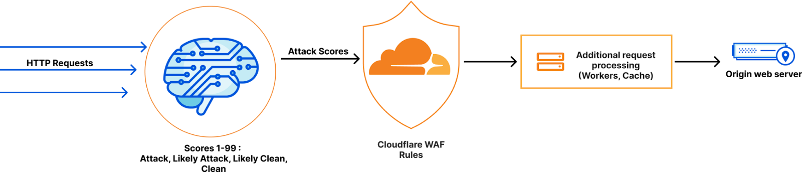
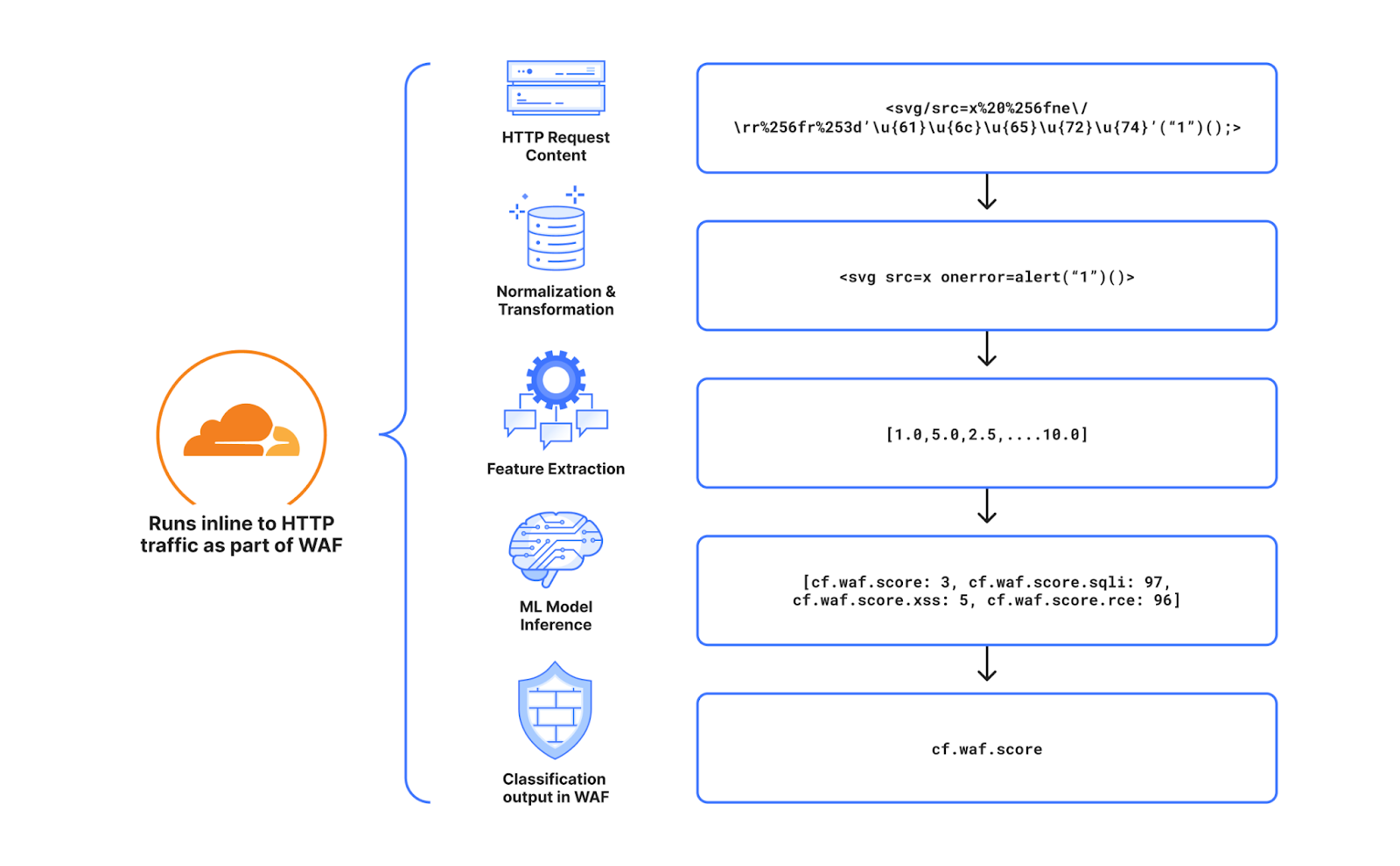
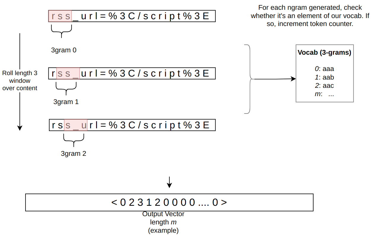
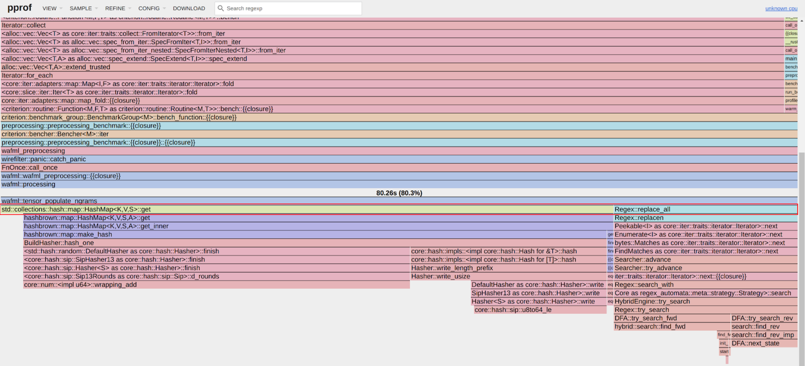


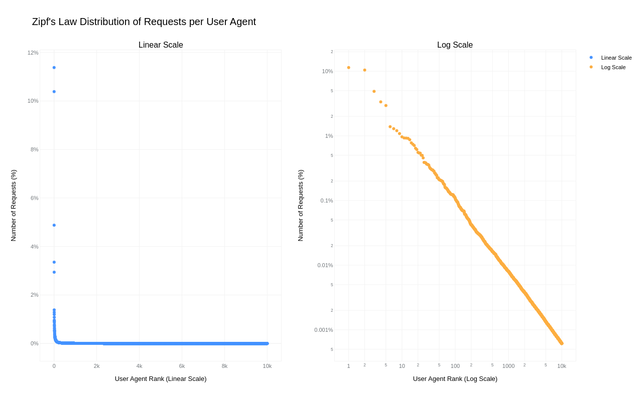
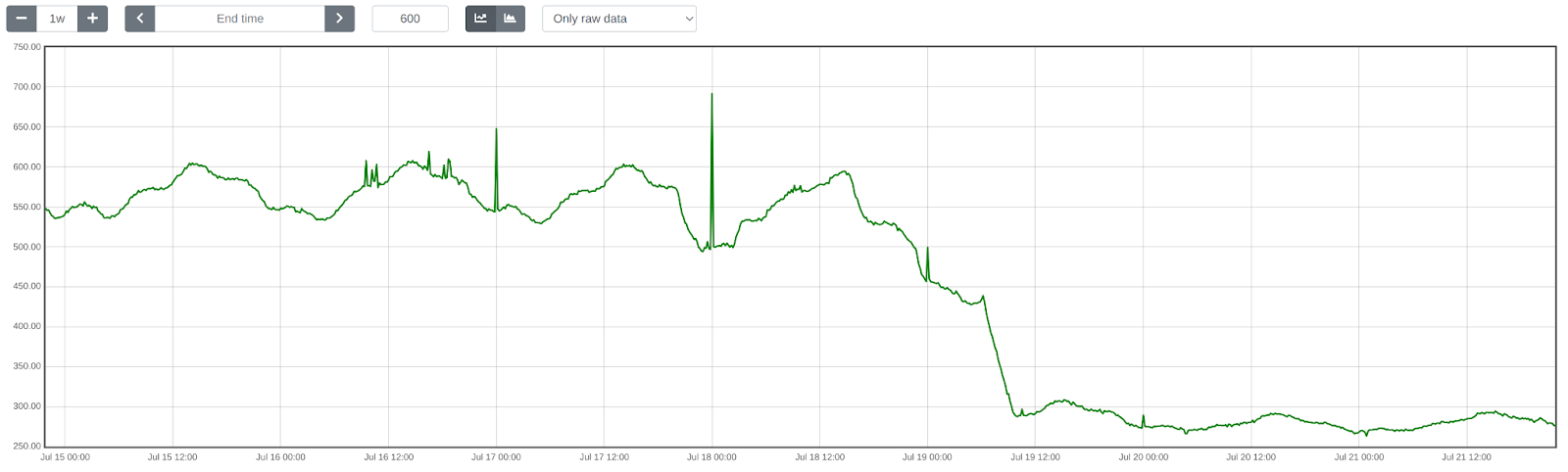


 Arpad Csoke is a Solutions Architect at Amazon Web Services. His responsibilities include helping large enterprise customers understand and utilize the AWS environment, acting as a technical consultant to contribute to solving their issues.