Въпросът на седмицата, който вълнува политическите наблюдатели в целия свят, е загуби ли Тръмп войната в Иран. Оценките са далеч от еднозначни, но дори сред привържениците на президента в Републиканската партия се чуха твърдения, че това развитие е най-тежката външнополитическа грешка на САЩ от десетилетия насам. Разбира се, тези оценки щяха да имат значение, ако и подписаният меморандум имаше значение – а в това никой не изглежда да е сигурен.
У нас също малко неща изглеждат сигурни. Все още няма представен бюджет, а почти преполовихме годината. Затова пък парламентът позволи на правителството да изтегли до 3,8 млрд. евро допълнителен държавен дълг за финансиране на бюджетен дефицит. Съвсем несигурни изглеждат и реформите, очаквани от кабинета Радев – и тези в държавната администрация, и тези в съдебната система. За сметка на това обаче доскорошният президент е пределно ясен по отношение на новия пакет санкции срещу Русия… с православни аргументи. Приоритети!
И Делян Пеевски изглежда непоклатим, макар и черупката на лидерството му в ДПС да се понапука напоследък. Рано е да проличи дали усилията му да обедини партията със законодателни предложения по теми, които са емоционални за мюсюлманската общност, ще спрат разпадането на локални структури и ще поправят слабия електорален резултат. Зависи от това дали „Прогресивна България“ ще успее да измести ДПС в местното управление, или българските турци ще продължават да гласуват както досега. Засега Пеевски олеква, но не достатъчно, за да потъне, смята Емилия Милчева.
Управляващата партия обаче не за първи път демонстрира, че прогресивността е само куха част от названието ѝ. Личи от декларацията ѝ в подкрепа на т.нар. Шествие за семейството. Това е онзи тип „подкрепа“, която избира „правилното“ и зачерква „неправилното“. Според Светла Енчева България навлиза в нов етап на отношение към човешките права и демокрацията – и по-точно заглавие на текста ѝ от „Добре дошли в държавния регрес!“ едва ли може да се намери.
Съвременните палиативни грижи не са „медицински грижи в края на живота“, а комплексен подход, който цели да направи живота на хората с тежки заболявания по-пълен и достоен, колкото и да остава от него. В България обаче това остава извън фокуса на публичния дебат и обществените политики. Липсват думи като „радост“ и „игра“, когато се обсъжда темата за детските палиативни грижи, а гласовете на самите деца и техните семейства почти не се чуват. Според Надежда Цекулова точно думите, които избираме да не включим в този разговор, показват в коя посока като общество сме решили да гледаме и какво остава извън полезрението ни. Непременно прочетете статията ѝ „Големият отсъстващ. Детските палиативни грижи в публичните политики и в публичния дебат“.
Как архитектурата се превръща в средство за инструментализиране на властта, е въпросът, който пулсира от всеки абзац на статията на арх. Анета Василева, която има късмета да наблюдава от първо лице началото на вълната от граждански протести против застрояването в Албания. Във фокуса на обществения гняв е лично Еди Рама, министър-председател и бивш кмет на Тирана, превърнал столицата в лаборатория за авангардни архитектурни проекти, но на фона на хаотично градоустройство и изключване на местните професионалисти от процеса. А т.нар. Фламингова революция е, от една страна, отчаян ход на съпротива на обикновените хора, а от друга, разкрива лицемерието на статукво, в което архитектурата е оръжие, но и жертва на политически амбиции.
За началото на лятото в рубриката ни на „Второ четене“ Антония Апостолова ни връща към един доста различен сборник с разкази. „Да си мъж“ на Никол Краус само на пръв поглед изглежда равен и сякаш безсъбитиен, докато дълбочината на прозата е скрита именно в липсите, празнините и неизказаните неща. Краус майсторски превръща микрокосмоса на семейното и интимното в универсални размисли за паметта, идентичността и времето. „Да си мъж“ е книга за това как човек свиква с непознатото, превръщайки го в част от себе си, и как паметта – и личната, и колективната – оформя същността ни. Според Антония това е сборник на човешкото оцеляване.
А като говорим за оцеляване чрез изкуство, за мнозина точно с музиката по-лесно се преглъща ежедневието. Как обаче да стане това, ако живееш в свят, в който музиката (особено западната) е „суетно забавление“, че даже отваря и врата към пороците и разврата. В рубриката си „Ориент кафе“ Атанас Шиников сблъска хевиметъла с исляма – два свята, осъдени на вечна раздяла. В първата част на „Къде е шейтанът тук?“ Аллах и тежка музика“ ще научим за корените на това негативно отношение на ислямските авторитети към музиката, но и защо дори в най-консервативните общности тя си пробива път. За втората част Атанас обещава да е запазил повече от същинското „главотръскане“. Нямаме търпение…
Не знам дали вече се разчу, но след множество прожекции и срещи с публиката в цяла България филмът на Лина Кривошиева „Какво е да остарееш в България“ вече е достъпен за свободно гледане в YоuТube канала на „Тоест“.
Качествената документалистика обаче не може да се прави без пари. Този филм беше финансиран по проект, но за следващата тема (и своеобразно продължение на разговора) с Лина имаме нужда от вашата подкрепа. Документалните филми са отделна част от нашата дейност и за тях винаги търсим самостоятелно финансиране, така че да не отклоняваме средства от всекидневната журналистическа работа. Включете се с дарение за краудфъндинг кампанията на „Тоест“ за новия ни филм „Какво е да си млад в България“. Всички средства от нея ще отидат директно за заснемането, озвучаването, историята и екипа, който ще я разкаже.
Част от вас може би вече дарявате всеки месец на „Тоест“. Тези средства осигуряват издръжката на медията – журналистическата работа, редакционния процес, комуникацията с публиката, развиването и поддръжката на сайта.
А ако все още не сте регистрирали редовно дарение на „Тоест“, направете го, за да може екипът ни да продължи да прави качествена журналистика за всички.
At Netflix, our catalog metadata is crucial to our member experience, and a single corrupted data state can impact millions of viewers immediately. To protect streaming reliability, we built an automated data canary system that validates data transformations using production traffic. This canary detects issues in under 10 minutes, and blocks bad data from reaching our members.
Intro
Catalog metadata is what makes Netflix functional. It defines what titles exist, where they’re available, whether they can be played, and more. This data gets transformed and distributed across our vast infrastructure near-continuously, powering everything that helps members find what they want to watch. Accurate catalog data delivers moments of joy. Corrupted catalog data breaks streaming.
What Went Wrong
A production incident revealed a critical gap in our resilience strategy. No code had been deployed. No configuration had changed. But, a manual mitigation action taken during a previous incident had inadvertently corrupted a data feed, rendering it empty for a subset of titles.
The impact was immediate: missing metadata prevented manifest generation, causing failures in our catalog service and playback issues.
Engineers were alerted immediately, but identifying the root cause took time. After intense triaging, responders pinpointed the corrupted data feed and pinned services back to a known-good state, restoring playback.
The problem? Our sophisticated code canary deployments had caught nothing. No code had changed — the data had.
This incident exposed a fundamental gap in our resiliency capabilities: we can validate code deployments, but we had no equivalent for our high-velocity data pipelines. Our catalog metadata, consisting of titles, artwork, availability, and more, was continuously transformed from multiple upstream sources and published at a regular cadence. Each upstream source had its own validation, but these checks didn’t catch corruption in the final transformed output.
We needed to treat data deployments with the same rigor as code deployments.
The Challenge: Validating Data at Short Intervals
Our catalog metadata service operates as a high-velocity data pipeline: it processes multiple input feeds, transforms them, and publishes the final catalog state that gets distributed across our infrastructure.
This creates unique validation challenges that our traditional canary analysis tools aren’t designed to handle:
Time Constraints: Our existing canary analysis tools require 30–60 minutes to reach statistical confidence. We had a much shorter window between data cycles; we needed to detect issues, make a decision, and block publishing all within a single cycle.
Emergent Issues: While each upstream data source has independent validation, problems often only manifest in the final transformed state. We needed to validate the actual output that clients would consume, not just the inputs, as close to the clients as possible.
Production Traffic is Essential: We initially considered shadow traffic, but quickly realized it was insufficient. Shadow traffic can only replay requests to our catalog metadata service; it can’t simulate the entire playback lifecycle across multiple services and domains. To detect real customer impact, we needed real production traffic.
Limit Blast Radius: Despite using production traffic for validation, we couldn’t allow customers to experience widespread issues during the validation process. Any regression needed to be detected and contained immediately.
Our Solution: The Data Canary Orchestrator Pattern
After evaluating several architectural approaches, we developed a solution built around three key innovations:
1. Dedicated Orchestrator Pattern
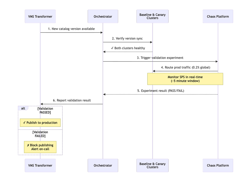
We created a dedicated cluster for the purposes of canarying new catalog metadata that separates concerns, avoids self-testing, and provides a pattern for extensibility. Here’s how it works:
Orchestrator Instance: A dedicated orchestrator instance of our catalog metadata service coordinates the data canary flow. When a new catalog version is published to the canary environment, the orchestrator validates that both baseline and canary clusters are healthy and version-synchronized, then triggers a chaos experiment.
Permanent Baseline & Canary Clusters: Two dedicated service clusters run continuously in our canary region. The baseline cluster always serves the latest production catalog version, while the canary cluster receives new versions for validation.
Generic Integration Point: Upon chaos experiment completion, the orchestrator reports results back to the transformer service via a REST endpoint. This generic interface means new data sources can implement their own orchestrator patterns without requiring transformer code changes.
This pattern can now be adopted by other teams at Netflix for validating different data sources, which is exactly the kind of extensibility we designed for.
Data Canary workflow
2. Utilizing and Extending our Chaos Platform
Meeting the 10-minute constraint required not only leaning on our chaos platform, but also extending it to meet our needs:
Custom Threshold Tuning: We worked with our Resilience team to customize experiment thresholds for our use case. Standard chaos experiment thresholds were too conservative for our time constraints.
Multi-Tenant Testing: Our catalog service supports multiple client types with different traffic patterns and downstream dependencies. We ran separate experiments for major client types and discovered that running traffic through the tenant that handles playback requests consistently identified failures fastest.
Sticky Canaries: To isolate experiment traffic, sticky canaries use session affinity to guarantee that once a user’s traffic is routed to the baseline or canary clusters, it stays there for the duration of the experiment window. This prevents cross-contamination from concurrent chaos experiments, ensuring a clean apples-to-apples comparison between data versions.
Behavioral Metrics Over Technical Metrics: We focused on Starts Per Second (SPS), or actual customer playback attempts, as our primary signal. SPS proved more reliable than latency or error rates for detecting catalog corruption because it directly measures customer impact, and data errors may not always manifest as application errors to our catalog metadata service.
Immediate Abort on Regression: Instead of collecting data for post-hoc analysis, we stream metrics in real-time and abort experiments the moment we detect regression. This trades some statistical confidence for speed, but our tight thresholds and clear signal make this not only acceptable, but necessary.
3. Production-Hardened Edge Case Handling
Building a system that runs in production every 10 minutes taught us that the devil is in the details:
In-Flight Experiments During Redeployment: When the orchestrator restarts, it must detect and continue polling any ongoing experiments, as we can’t abandon a validation cycle mid-flight.
Leader Election: During orchestrator deployments, multiple instances might be running simultaneously. We implemented safeguards to ensure only one experiment is triggered per version announcement.
Version Synchronization: In a multi-tenant service where different clients consume data at different cadences, we track version state to ensure baseline and canary clusters are properly aligned before triggering experiments.
Validating the Validator: Controlled Failure Injection
To prove the system worked, we needed to break things on purpose. We ran a series of controlled experiments where we deliberately corrupted catalog data — denylisting high-profile titles and simulating real data corruption scenarios — to validate that the canary could detect issues and block publication.
These experiments were coordinated as proactive incidents during business hours, with product operations teams on standby. We routed approximately 0.2% of global traffic through the validation flow, minimizing blast radius while still generating meaningful signal.
Key Results:
Detection Speed: Issues identified in 2.5–4 minutes depending on client type
Clear Signal: 10x error differential between canary and baseline
Automatic Blocking: Publishing workflow blocked as designed when regressions detected
The experiments validated our end-to-end workflow and revealed important operational insights: different client traffic patterns detect failures at different speeds, and threshold tuning requires careful refinement based on the magnitude of impact we want this system to detect. Most importantly, they proved that even with a 10-minute validation window, far shorter than traditional 30–60 minute canary analysis, we had sufficient signal to catch high-impact catalog corruption.
Bringing Code Validation Principles to Data
This effort wasn’t just about building a validation system, it was about recognizing that data deployments deserve the same rigor as code deployments. Just because something isn’t a binary doesn’t mean it can’t break production. The patterns we landed on aren’t specific to catalog metadata, and can be applied to systems with high-velocity data pipelines more broadly.
If you’re working with data that changes frequently and impacts customers directly, ask yourself:
What’s your MTTD for data corruption?
Can you validate with production traffic safely?
How would you detect emergent issues in transformed data?
What behavioral metric most closely indicates customer impact in your domain?
Today, the failure mode that caused the aforementioned incident would be caught and mitigated in under 10 minutes. We all know outages aren’t a question of if, but when. The next time you find yourself faced with bad data, how fast will you be able to respond?
Acknowledgments
This work was a collaborative effort across multiple teams at Netflix. Special thanks to Jongyoon Lee, David Su, and Zubeen Lalani of the Catalog Foundations & Distribution team for their contributions to the design, and to Ales Plsek of the Resilience team for their support in customizing our chaos platform for our unique use case.
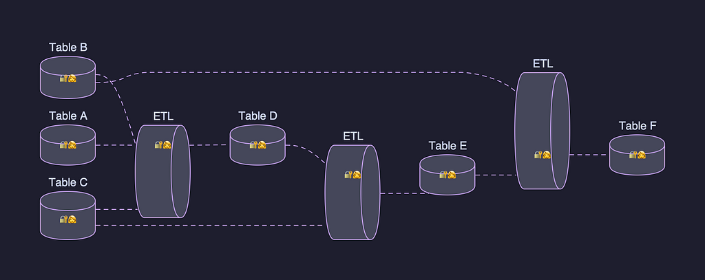
Netflix’s Data Platform is vast. We have millions of tables in our data warehouse and tens of thousands of scheduled workloads running across our orchestration systems. Behind each of these assets sits an engineer, a team, or an initiative — and behind each of those sits a set of decisions about who can access what, and how those workloads execute day after day.
For years, the tools we used to manage access and identity for these assets operated at the granularity of the individual asset. Every table had its own Access Control List (ACL). Every workflow ran under the identity of the engineer who authored it. In a workforce that is fluid, where people change teams, change roles, and occasionally leave the company, this fine-grained model broke down in two persistent, painful ways.
Problem 1: Permissions that can’t keep up with organizational changes
Imagine you’re on a team that owns a few hundred tables. Your org restructures, a neighboring team merges into yours, and you inherit another few hundred. Now you have to find every ACL on every table, figure out who should still have access, and update them one by one. Multiply that by every reorg across every team across the company. The result? Two failure modes:
The support team gets flooded. A significant and outsized share of support threads were requests to update table permissions en masse in response to org changes. While self-service tooling and best practices are in place to manage this, adherence is inconsistent. Data Projects addresses this by promoting the solution from optional tooling to a foundational part of the data platform.
Access gets granted far too broadly. Rather than maintain fine-grained ACLs, teams would often open up table access to the whole company. This defeated the purpose of having ACLs in the first place.
Problem 2: Workloads tied to human identities
Scheduled and asynchronous workloads — Maestro workflows, data movement jobs, Spark pipelines — need an identity to run as. Historically, that was a human: whoever authored the workflow.
Human identities are not durable. People change teams, get new responsibilities, and leave the company. When they do, their permissions change, and the workflows running under their identity start to fail. The only fix was to swap in a colleague’s identity, which inevitably had different permissions, kicking off a “permissions whack-a-mole” as each fix surfaced the next missing grant. And then, eventually, that colleague would also move on, and the cycle would repeat.
Enter Data Projects
We introduced Data Projects to tackle both problems head-on. At its core, a Data Project is two things:
A container to manage and view a set of related assets in aggregate: tables, workflows, and other data assets grouped under a single logical umbrella.
A synthetic, durable, and assumable identity: one that asynchronous and scheduled workloads can execute under, independent of any human’s lifecycle.
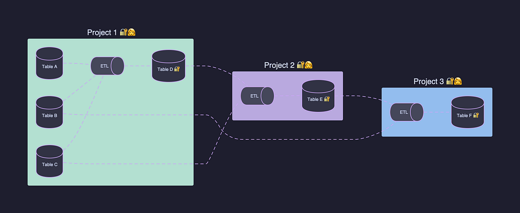
You can think of it as hoisting the granularity of management up from the individual asset to a meaningful container: the project. Instead of managing permissions on 500 tables, you manage them on one project that contains those 500 tables.
While the initial focus has been access and identity, the abstraction has applications well beyond those concerns. That broader potential is part of what makes it worth investing in.
Figure 1a. Individual assets, each managed in isolation, with per-asset access controls and per-person ownership.Figure 1b. These assets are logically grouped into projects for easier management.
Grants and Roles
Each Data Project has a set of grants managed by the owning team. Different identity types can be added as grants: users, groups, applications, and continuous integration (CI) jobs. Each grant has a role that determines what the grantee can do within the project. For example, a Contributor has read/write access to the project’s assets, while a Viewer has read-only access. These roles roll up neatly — instead of rewriting hundreds of ACLs when someone joins or leaves a team, you update a single project grant.
The Identity Umbrella: Netflix and IAM
Every Data Project is provisioned with a Netflix application identity, and optionally an AWS IAM role. This is the “identity umbrella” that makes workloads durable:
The project’s Netflix identity is what executes the project’s async workloads (e.g. Maestro workflows). It belongs to the project, not to any person.
The project’s IAM role supports specialized use cases in AWS like Spark jobs on Amazon EMR. Crucially, the IAM role can be exchanged for the project’s Netflix identity in a cryptographically secure way.
Members with privileged roles can also assume the project’s Netflix identity. This is enormously useful for testing and troubleshooting from a development context like a laptop or a notebook — you get to run commands as the project, exactly as the scheduled workload would.
Gravity
One of the more elegant properties of Data Projects is what we call gravity. When a workload running under a project’s identity creates a new asset — say a Maestro workflow creates three tables — those assets are automatically added to the project as contained assets. The project becomes the center of mass for everything produced under its identity. You get organization for free as a side effect of how the platform already works, eliminating future challenges of discovering relevant assets and gaining access to them.
Securing Data Workflows with Data Projects
Maestro is Netflix’s primary workflow orchestrator for batch analytics, covering scheduled ETL pipelines, data movement jobs, ML training, and much more. Because workflows can run on schedules without the original user present, Maestro is designated a Trusted Workload Manager (TWM), formally authorized to mint fresh identity tokens on behalf of the workloads it manages.
That identity matters everywhere. A single workflow execution may be checked against table ACLs in the Secure Data Warehouse, authorization policies for Netflix resources, and IAM policies for AWS — all in a single run. If the identity is fragile, the whole workflow is fragile.
The Problem with User-Tied Identity
The standard pattern was to run workflows under an On-Behalf-Of (OBO) credential — for example, maestro OBO [email protected]. This gave the workflow the union of Maestro’s and the human’s permissions, but in doing so it also bound the workflow’s permissions to that person’s. When they changed teams or left Netflix, the workflow broke. A colleague might take over ownership, but they rarely had the same access as the previous owner, so the workflow would stay broken for days while permissions were sorted out. At Netflix’s scale, with tens of thousands of scheduled workloads, many of them business-critical, this was unsustainable.
Data Projects: Durable Identity
Data Projects solves this by replacing user-tied identity with a durable, team-owned Netflix application identity: one that doesn’t change teams, go on vacation, or leave the company. Each project groups related workflows, tables, secrets, and other assets under a single consistent identity, and Maestro validates the caller’s access to the project before executing any workflow under it.
The downstream improvements are as follows:
Tables created during execution are automatically associated with the project’s identity through gravity, inheriting its access controls without additional configuration.
Secrets are scoped to project policies, so ownership transfers no longer strand credentials.
Access is managed once at the project level, replacing fragmented per-user grants across every asset the workflow touches.
The result is a workflow identity model that is stable, auditable, and built to survive the organizational changes inevitable at any company operating at this scale.
Success Stories
Many Data Projects have already grown to contain tens of thousands of assets in production. A couple examples are highlighted below:
Streaming Quality of Experience: A core observability pipeline tracking quality of experience (QoE) metrics whose continuity used to depend on whichever engineer happened to own the underlying workflows. Now it runs under the project’s identity, stable regardless of team membership changes.
Member Analytics: Analytical models and ETL workflows for member data products. A concentrated set of business-critical analytics whose access is managed at the project level rather than across hundreds of individual tables and workflows.
More broadly, we’ve seen Data Projects adopted as the organizing principle for entire analytics domains. Where teams previously maintained their own access policies, ad-hoc grant lists, and tribal knowledge about “who should have access to what,” the project is now the single answer.
Using Data Projects
Onboarding workflows onto Data Projects is a matter of:
Creating a project for the logical grouping of assets (or using an existing suitable one).
Granting the right people and groups the appropriate roles.
Configuring the workflow to run with the project’s identity.
Thanks to gravity, new assets produced by project workflows land in the project automatically. Migrating existing workflows can be a challenge as it requires setting up the Data Project with the appropriate permissions before changing its execution identity. We are actively working on infrastructure to track the access patterns of existing workflows so that we can recommend precise permission updates for the destination project. Our goal is to make the Data Project the de facto option for executing any kind of asynchronous workload.
What’s Next
Data Projects started as an Analytics Platform initiative, a response to specific pains in the data warehouse, but the underlying ideas are not unique to data. We see a potential future where Projects (not just Data Projects) are a first-class platform concept spanning data assets, software assets (GitHub repositories, Spinnaker applications, Docker images), and even studio assets (production content, pipelines, and transformations).
We’re also investing in:
Rightsizing: we’re integrating a layer on top of our authorization policies that automatically rightsizes permissions based on actual usage patterns, proactively eliminating unnecessary access and preventing “permission creep”.
Hoisting beyond access and identity: the project is a natural unit for surfacing other concerns at the aggregate level — cost attribution, health indicators, and more.
Ad-hoc use case integrations: extending project identities beyond scheduled workloads to cover interactive, on-demand actions like running a query through the Data Portal.
Activity logs and audits: a unified timeline of grant changes, asset changes, and workflow versions at the project level.
Conclusion
Data Projects is an answer to a simple observation: at Netflix’s scale, the unit of identity and access management can’t be the individual asset or the individual human. It has to be something larger, something durable, something that matches the way teams actually think about the work they own.
A project is that unit. And as we continue to generalize the concept beyond the data warehouse, we expect it to become one of the foundational primitives of how engineering at Netflix is organized, not just how data is organized.
Acknowledgments
We would like to express our gratitude to the following individuals for their contributions to this effort: Ryan Bordo, Doug Clark, Luke Fernandez, Sarrah Figueroa, Ankit Gupta, Brian Hoying, Ye Ji, Abhishek Kapatkar, Anmol Khurana, Matheus Leão, Hechao Li, Raymond Liu, Alice Naghshineh, David Noor, Anjali Norwood, Javier Garcia Palacios, Kunaal Parekh, Brandon Quan, Andrew Seier, Jason Seo, and Ethan Zhang.
If you are interested in helping us solve these types of problems and helping entertain the world, please take a look at some of our open positions on the Netflix jobs page.
Each year, we bring the Analytics Engineering community together for an Analytics Summit — a multi-day internal conference to share analytical deliverables across Netflix, discuss analytic practice, and build relationships within the community. This post is one of several topics presented at the Summit highlighting the breadth and impact of Analytics work across different areas of the business.
Understanding Risk in Content Launches
Every title you see on Netflix goes through several key phases: Development, Pre-Production, Production/Principal Photography, Post-Production, and finally, Launch Preparation, all leading up to the Title Launch. Once Principal Photography wraps, the focus shifts in Post-Production from content creation to quality assurance and visual effects (if needed).
At the end of Post Production, Netflix receives the final audio and video files — often delivered as an IMF (Interoperable Master Format) — which triggers a flurry of Launch Preparation activities, focused on tasks such as the development of artwork and trailers, creation of subtitles, maturity ratings & quality control, that happen within a tight window and rely on having the finalized media assets in hand.
Some of this work can be kicked off earlier using a non-final version of the media called the Locked Cut, but since it’s not the absolute final deliverable, this presents a tradeoff: should our teams who prepare content for service wait for the more finalized IMF to begin their work, or start sooner with the unfinal Locked Cut? Waiting for the IMF risks a compressed timeline if it arrives late, while starting with the Locked Cut means teams may need to do additional conformance work if there are significant changes between the Locked Cut and the final IMF.
Identifying Gaps in Schedule Accuracy
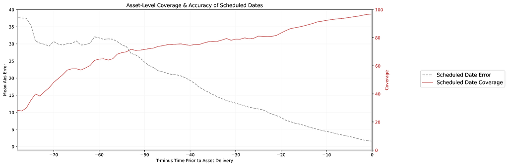
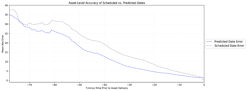
To help navigate the decision of when to start launch preparation, our teams rely on estimated delivery dates for both the Locked Cut and IMF media assets, which are manually provided by content partners in production schedules. However, these schedules often have gaps in coverage and lack accuracy for both asset types (see Figure 1).
Figure 1. At an asset-level we generally see that scheduled date accuracy and coverage are lower at horizons further from asset delivery. As we approach delivery (moving towards the right on this plot) schedules become more accurate (errors decrease) adn coverage improves.
This isn’t unexpected — productions are dynamic, facing frequent changes, scheduling conflicts, and unforeseen obstacles that can shift timelines without warning. As a result, there’s a clear opportunity to leverage the wealth of production data we collect to predict the risk of schedule slips. By developing a predictive model, we aim to both fill in ETA gaps (providing asset delivery estimates when none exist) and improve the accuracy of existing ETAs compared to traditional manual schedules.
Correlation between Schedule Accuracy and Launch Misses
Our analysis reveals a strong correlation between scheduled inaccuracies and launch misses — instances where a title experiences delays. To quantify schedule inaccuracy, we created a metric called Accumulated Error Days (AED), which measures the cumulative deviation between estimated (scheduled or predicted) delivery dates and actual delivery dates over time. AED is calculated retrospectively as the area between the scheduled (grey line) or predicted (blue line) delivery dates and the actual delivery date (green line).
When we compare titles with at least one launch miss to those without, we find that mean AED is significantly higher in the group with launch misses. Notably, this effect is even more pronounced when we focus on the period closer to delivery — indicating that high AED (i.e., inaccurate schedules) in the final stretch before launch is especially correlated with launch misses, more so than AED accumulated over a longer timeline. These findings further motivate our efforts to improve schedule accuracy and reduce AED by leveraging rich production data and predictive modeling.
Modeling Time-to-Delivery
Our predictive models are designed as boosted tree regression models that predict the “days until” either media asset delivery for in-progress productions.
To power these models, we leverage a range of upstream data sources including production-level signals of progress, title metadata, and seasonal signals. We are able to predict the days until media asset delivery using daily update snapshots, allowing us to generate up-to-date predictions that reflect the latest state of each in-progress production. This means that we have each feature and what its value was as of each day of a production. Modeling with this snapshotted data enables us to generate up-to-date predictions as new information becomes available, build a flexible model that works across all production phases, and seamlessly incorporate dynamic features that evolve over time (Figure 2).
Figure 2. Hypothetical illustration of the evolving nature of production-related signals used in our models. Some signals are present throughout but dynamic, others are present at single moments in time during specific production phases. By capturing data in a snapshotted form, we’re able to build a flexible phase-agnostic model that leverages many different types of progress signals. This figure is illustrative only and does not depict actual Netflix financial or production data.
Evaluating Our Approach
Building a Comprehensive Metrics Suite
When evaluating the performance of the predictive models, we look across a suite of metrics to try to understand where and when predicted dates outperform scheduled dates. Among these are mean and median absolute error, relative to actual delivery, to understand the accuracy of our estimated dates. We also consider bias metrics, such as mean and median error, to understand if we are consistently over- or under-predicting the actual delivery. We calculate the standard deviation of our errors to understand if there are large shifts in the bulk of the distribution of errors. For the tails of our error distributions, we calculate the percentage of our absolute errors that are greater than x days to delivery.
For scheduled dates, we calculate coverage across various horizons to delivery. This is a value prop of the model; we’ve built the model in such a way that we can always provide a predicted date and recoup any coverage gaps that exist from scheduled dates alone.
Benchmarking Against Manual Scheduling
In a backtest, we observed significant improvements across all of our metrics and across most horizons from delivery. As an example, see Figure 3 which plots global mean absolute error (MAE) and shows large reductions in errors (greater accuracy) in predicted IMF and Locked dates as compared to scheduled dates. Additionally, we see large reductions in outliers from scheduled to predicted dates as well.
Figure 3. This plot compares accuracy (measured as Mean Absolute Error) between predicted and scheduled dates. The horizontal axis plots time prior to delivery, which decreases from left to right until you reach the moment of delivery at the bottom right. For this particular asset, the predicted delivery dates on average are much more accurate than manually scheduled delivery dates throughout the full horizon to delivery.
Since our teams use these dates over a period of time and not at a single point in time, there is an additional benefit that we’re describing as an Earlier Accuracy Signal. By leveraging predictive dates, our teams benefit from a level of accuracy that they would otherwise have to wait x amount of time for if using scheduled dates. As an example, 6 months out from Locked Cut delivery the predicted dates are better than scheduled dates on 76% of titles and have a level of accuracy (6.1 wks MAE) that scheduled dates don’t reach until 11 weeks later.
Circling back to AED, which we mentioned earlier is correlated to launch misses, we find that in our backtested titles globally, and across most buying orgs and content types (i.e., series versus standalones), predicted IMF and Locked Cut dates reduce AED from scheduled dates when calculated across the 6 months leading up to delivery. We see similar patterns when we repeat this for shorter horizons to delivery as well.
Streamlining Workflows with Improved Scheduling
A key advantage of this predictive model is that estimated delivery dates are already integral to our stakeholders’ workflows — meaning we can introduce predictive dates without overhauling existing processes. However, this creates a new challenge: with both scheduled and predicted dates available, teams need to determine which is more reliable. While predictive dates are often more accurate on average, there are situations where scheduled dates perform better. To address this, we’ve built serving logic that defaults to scheduled dates in buying orgs where the model underperforms. Elsewhere, teams can view both dates side by side in dashboards, allowing them to apply their own judgment. Additionally, our predictive models leverage features that are tied to scheduled dates, which has emphasized the need and impact of ensuring our upstream teams continue to input and update scheduled dates even in the presence of our predictions. We’re piloting these predictive signals in multiple ways, tailoring the approach to fit the diverse needs and tools of our various launch prep functions.
In a previous post, we introduced Data Bridge, a unified management plane for batch Data Movement at Netflix. Historically, several bespoke Data Movement connectors were developed across different engineering organizations to fulfill their specific requirements. Over the last few years, the Data Movement team has started centralizing these offerings through an abstraction that provides a catalog of connectors, along with simple UI and APIs to initiate Data Movement jobs.
One such case is the Cassandra to Iceberg connector. Apache Cassandra powers mission critical applications at Netflix, including Member, Billing, Recommendations, Subscriptions and many more. These use cases heavily leverage Data Movement to Apache Iceberg for many analytics and operational tasks, and central to this movement was a connector for Cassandra to Iceberg built in-house named Casspactor. As many Cassandra based Data Abstractions emerged, such as Key Value, Time Series and Graph — the need for larger and more complex Data Movement with transformations became more critical to the business.
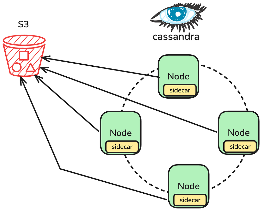
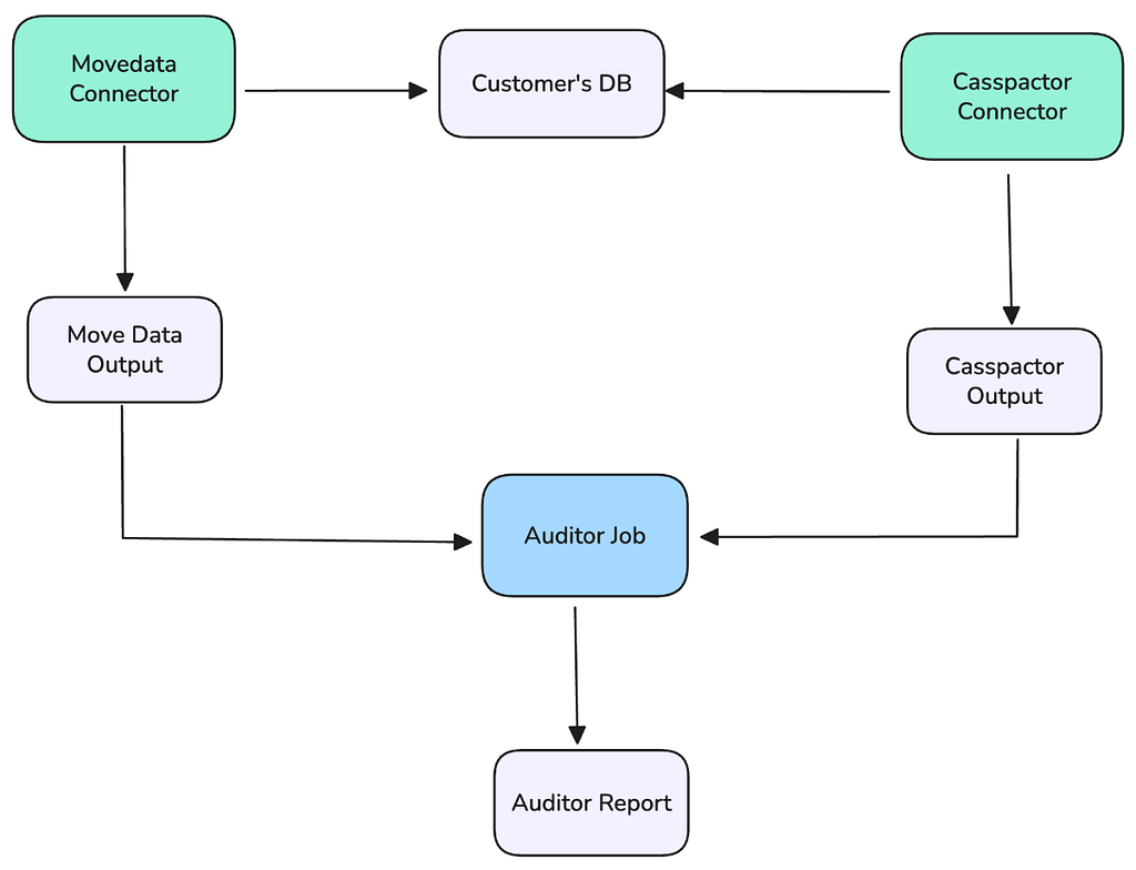
Data movements are fundamentally fulfilled by leveraging the existing Cassandra backup infrastructure. Regularly scheduled backups are performed directly on the Apache Cassandra nodes, via a sidecar process managing the upload of all necessary SSTables and associated Metadata files directly into Amazon S3. When a Data Movement job is initiated, the job constructs the specific backup structure it needs by referencing the S3 based metadata, allowing it to precisely locate the SSTable files. The engine then downloads these files, performs the required mutation compaction and processing, and finally writes the fully transformed, compacted data directly into the target Apache Iceberg tables.
Image 1: Cassandra Cluster Backups to S3
Casspactor: The Engine We Outgrew
Casspactor processed roughly 1,200 data movements per day, transferring approximately 3 PB of data from Apache Cassandra into Apache Iceberg tables. It served some of the most critical workloads at Netflix. For years, it worked. Then, two compounding challenges made it clear we needed a fundamentally different architecture.
Fragile Metadata Dependencies
Before Casspactor could move a single record, it needed to answer a deceptively simple question: which backup exists, is it complete, and what does it contain?
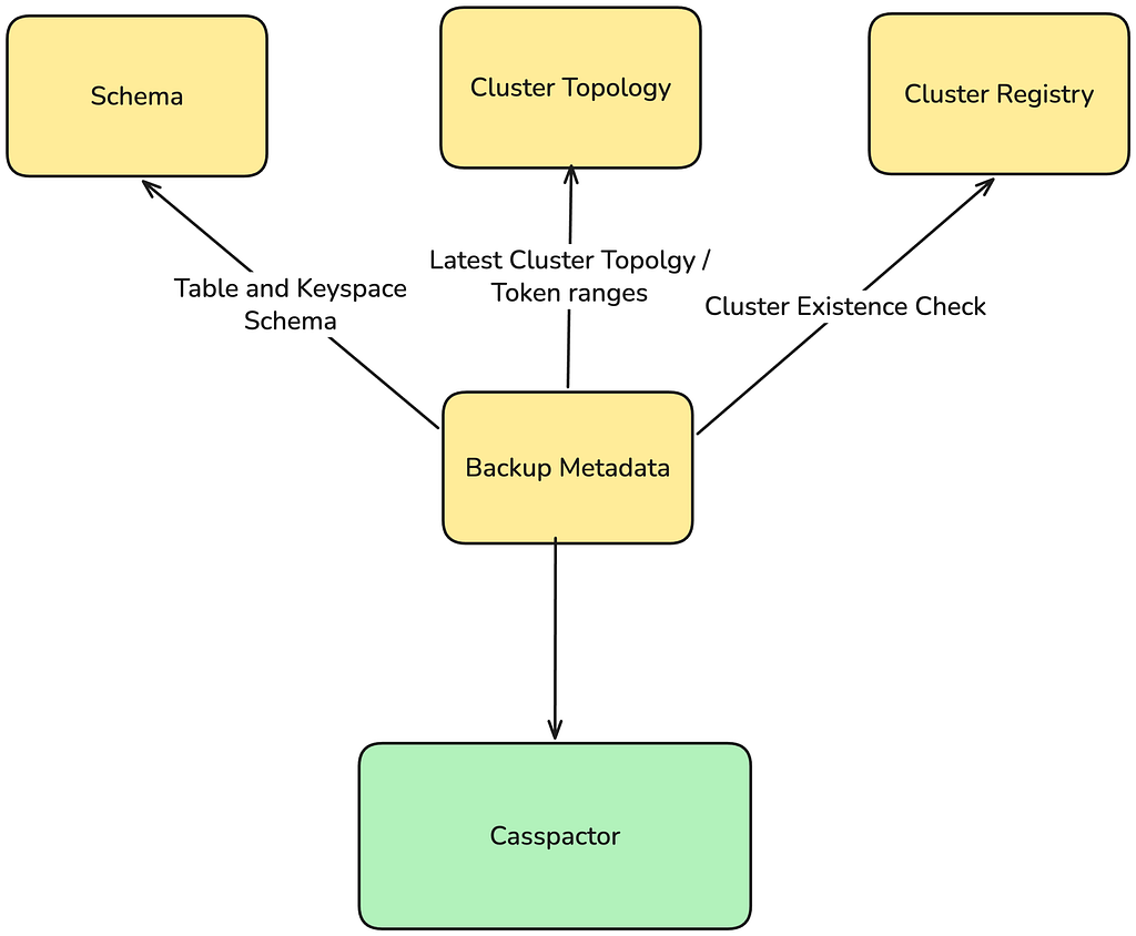
Casspactor assembled this answer from multiple independent systems:
Image 2: Casspactor’s Composite View of a Backup
Each system had its own failure modes, update cadences, and accuracy guarantees. Casspactor’s view of the world was a composite, and composites diverge from reality.
Metadata fell out of sync with actual backups, causing Casspactor to read stale or incorrect data silently. Routine maintenance on the Cassandra Clusters triggered uncoordinated snapshots, and because Casspactor required all nodes in a region to snapshot at the same clock second, a single node replacement could break data movement for an entire region.
The fix was hiding in plain sight. The answer to “which backup exists and is it complete?” already lived in the backup storage layer (Amazon S3) itself. By reading metadata directly from the backup files, we could replace the entire dependency chain with a single source of truth.
Every Connector Inherited Casspactor’s Limitations
Cassandra at Netflix does not just store raw tables. It backs higher level data abstractions, such as Key Value, Time Series, and others, each with its own data model, access patterns, and semantics. When any of these abstractions needed to move data to Iceberg, they all funneled through Casspactor.
Every abstraction inherited Casspactor’s constraints:
Skewed partition failures: Casspactor could not handle tables with large partitions, a common pattern in Key Value and Time Series workloads. Jobs crashed with out-of-memory errors on some of Netflix’s largest datasets.
No data model awareness: Casspactor moved raw Cassandra tables as is. Connectors for Key Value and other abstractions had to bolt on post processing to reconstruct their data models from the raw output — extra cost, extra complexity, and an extra surface for failures.
Intermediate table bloat: Casspactor wrote to an intermediate Iceberg table before producing the final output. The Key Value connector added another intermediate table and a snapshots table. Connectors for abstractions on top of Key Value added even more. This compounded into significant storage cost overhead.
Inability to Time Travel: by relying on multiple services to compose a backup unit, Casspactor was unable to restore prior backups in the event of cluster Topology or Keyspace schema changes.
Monolithic design: Casspactor was built as a single connector, not as an engine. There was no way to build a family of purpose built connectors on a shared foundation.
We needed something fundamentally different: an engine that reads directly from backups in S3, produces standard Spark DataFrames, and lets each data abstraction build its own connector with full awareness of its data model. One foundation, many connectors.
The New Stack: A Layered Architecture
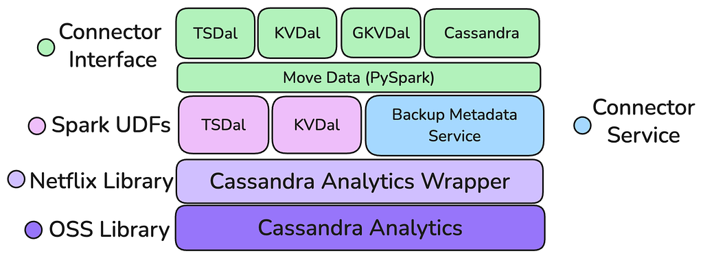
The new architecture, built upon the foundation of Apache Cassandra Analytics and the in-house Move Data framework, represents a fundamental shift toward a layered, purpose-built stack designed for reuse and maintainability. This new engine was conceived with clear separation of concerns, moving away from Casspactor’s monolithic design. The architecture is intentionally layered with the foundation being a core S3 reading capability: the Cassandra Analytics Wrapper, which is built on top of the Open Source Cassandra Analytics with Netflix’s internal backup representation and an S3 Client.
This layer handles the raw data retrieval from backups, translating it into standard Spark DataFrames. Sitting atop this foundation is a “Connector Factory” model, via both Java UDFs and transforms which allows individual data abstractions (Key Value, Time Series, others) to build highly optimized, data model aware connectors that process the generic Spark DataFrames, avoiding the need for complex, expensive, and failure-prone post-processing steps. This layered approach ensures that improvements to the core reading engine benefit all connectors, while the connectors themselves are focused solely on data transformation.
Image 3: The new Connector layered stack
Handles Skewed Partitions: By moving the mutation compaction and processing to the Executor level within Spark, the new engine can efficiently handle tables with highly skewed or wide partitions, a major pain point for Casspactor. Crucially, this processing occurs without excessive data shuffling, preventing out-of-memory errors and enabling reliable movement of Netflix’s largest datasets.
Operates at Spark DataFrames (No Intermediary Tables): The new architecture directly generates standard Spark DataFrames from the Cassandra backups. This eliminates the need for Casspactor’s costly, multi-stage intermediate Iceberg tables, which led to storage bloat and operational complexity. This native DataFrame operation enables the “Connector Factory” by providing a universal, easily consumable interface for building diverse, model specific connectors.
Jobs Auto Size: The engine integrates intelligent auto-sizing capabilities, allowing jobs to dynamically adjust resource consumption based on the source table’s characteristics. This removes the burden of manual tuning from engineering teams, ensuring optimal performance and cost efficiency without sacrificing reliability.
Reduced Dependencies: By reading metadata directly from the backup files stored in S3, the new stack removes the fragile, multi-service dependency chain that plagued Casspactor. S3 becomes the single, authoritative source of truth for backup existence and completeness, vastly improving data movement reliability and consistency.
Time Travel: A critical feature of the new stack is the ability to process the schema, cluster topology, and data as a cohesive unit at a specific point in time. This capability provides robust time travel functionality, essential for auditing, debugging, disaster recovery and reproducing past data states.
Performance: Collectively, these architectural improvements, including native DataFrame processing, optimized partition handling, and streamlined metadata retrieval have resulted in notable performance gains, reducing overall data movement execution runtime and cost compared to the legacy Casspactor system.
Cost: by eliminating intermediary Iceberg tables and efficient SSTable compaction on Executors, the new stack needs a significantly smaller storage and compute footprint leading to significant cost savings in the order of USD millions.
The Journey Towards a Safe Migration
The successful validation of the new stack was the critical first step, but it only marked the beginning of the most challenging phase: the migration. Large scale data migrations are inherently complex, high-risk undertakings that can be time consuming and often result in customer frustration and service disruption. To navigate the high stakes of decommissioning a mission-critical system like Casspactor and seamlessly replacing it, we needed a strategy that prioritized reliability and transparency above all else.
The migration was fundamentally enabled by a Like-for-Like strategy, which served as the cornerstone of our Platform Engineering philosophy, abstracting complexity. The core tenet was to maintain absolute consistency across the user-facing interface, the output contract, and the final data artifact. This meant ensuring that the data movement parameters defined via the Data Bridge abstraction remained unchanged, and, critically, the schema, metadata, and data within the destination Iceberg tables were identical to the legacy output. By preserving these external contracts, we eliminated the need for complex, time-consuming coordination with dozens of internal teams who relied on these data pipelines. This approach transformed the migration from a distributed, high-risk, multi-team effort into an internal platform implementation detail, allowing us to achieve a transparent, zero-impact transition and accelerate the retirement of the legacy system without requiring any code changes or validation from downstream users.
To navigate this migration, we developed a strategy anchored by three core pillars that serve as a blueprint for successful, large-scale data migrations:
Validation: Establishing and maintaining absolute confidence in data consistency through rigorous, ongoing validation.
Visibility: Instrumenting every part of the system to provide a clear, real-time understanding of migration progress and system health.
Safety: Ensuring user impact is minimized or eliminated, despite the inevitable system failures, by leveraging abstractions and robust fallbacks.
The next section will provide a detailed exploration of these key pillars.
Pillar 1: Validation
Trust is earned, and in data migration, it is earned one row at a time. The first pillar is the most critical: providing a measurable guarantee to users and partners that the data produced by the new system is an exact, row-by-row replica of the data produced by the old one.
Our foundational tactic was deploying the new Move Data connector in a “shadow” testing that ran in parallel with the production Casspactor jobs. This allowed us to validate the new system with real-world, production workloads without any customer impact.
Image 4: Shadow job structure leveraged for data validation
Let C be the set of rows in the legacy Casspactor output (Iceberg table).
Let M be the set of rows in the new Move Data output (Iceberg table).
The test for trust: prove that C = M. This required continuously checking for two conditions:
Rows in C but not in M (C-M): The new system missed data.
Rows in M but not in C (M-C): The new system introduced phantom or erroneous data.
Any result where the cardinality of these difference sets (the number of differing rows) was greater than zero triggered an immediate, high-priority investigation. The target was 100% similarity.
Uncovering and Resolving Disparities
The shadow mode quickly became a powerful forensic tool, exposing “unknown unknowns”, subtle discrepancies that were not bugs in the new system but rather differences in behavior between the new and old systems. Resolving these was the core work of building trust. For each problem we initiated an investigation log where we captured the details, logs, queries that allowed us to diagnose. Based on the assessment the issues were categorized so that similar differences on other datasets were later resolved affecting many of the shadow pipelines.
Maintaining an investigation log was critical to organize the outstanding issues and effectively communicate to stakeholders the progress and confidence of the new connector so that we effectively measure the appropriate level of “confidence” to initiate the migration.
We observed differences in how connectors leverage reference timestamps for Time-to-Live, Consistency Levels, backup selection, and various internal business logic. This continuous, data-driven cycle of discovery and resolution was the mechanism by which we built confidence in the new architecture.
Pillar 2: Visibility
Trust is built in the background, but an active migration requires real-time insight: Visibility. The second pillar involves instrumenting the system to provide an unambiguous, clear understanding of operational health and migration progress.
We extended our instrumentation to the overall migration workflow and its dependencies:
Dashboards: We created centralized dashboards to track migration status, visualizing the total number of data movements migrated versus those remaining. The dashboards tracked execution status, average runtime, and cost comparisons between the two connectors.
Dependency Tracking: Since the new system relied on a new set of APIs to fetch backup metadata, we implemented detailed metrics for failures to keep track of the APIs or dependencies failed.
Alerting: Proactive alerts were set up for job failures (Move Data or Casspactor), failures on Move Data that triggered a fallback to Casspactor or any data discrepancy being detected.
This comprehensive instrumentation allowed the team to be proactive, fix issues as they emerged during the migration, and gain the necessary confidence to accelerate the migration timeline.
Pillar 3: Safety
Even with perfect data correctness and enhanced visibility, the third pillar, Safety is required for a zero-impact migration. The challenge is ensuring that when a system inevitably fails, the user experience is uninterrupted. Our strategy centered on decoupling the user’s workflow from the underlying connector implementation.
Leveraging Abstraction: The Decider Pattern
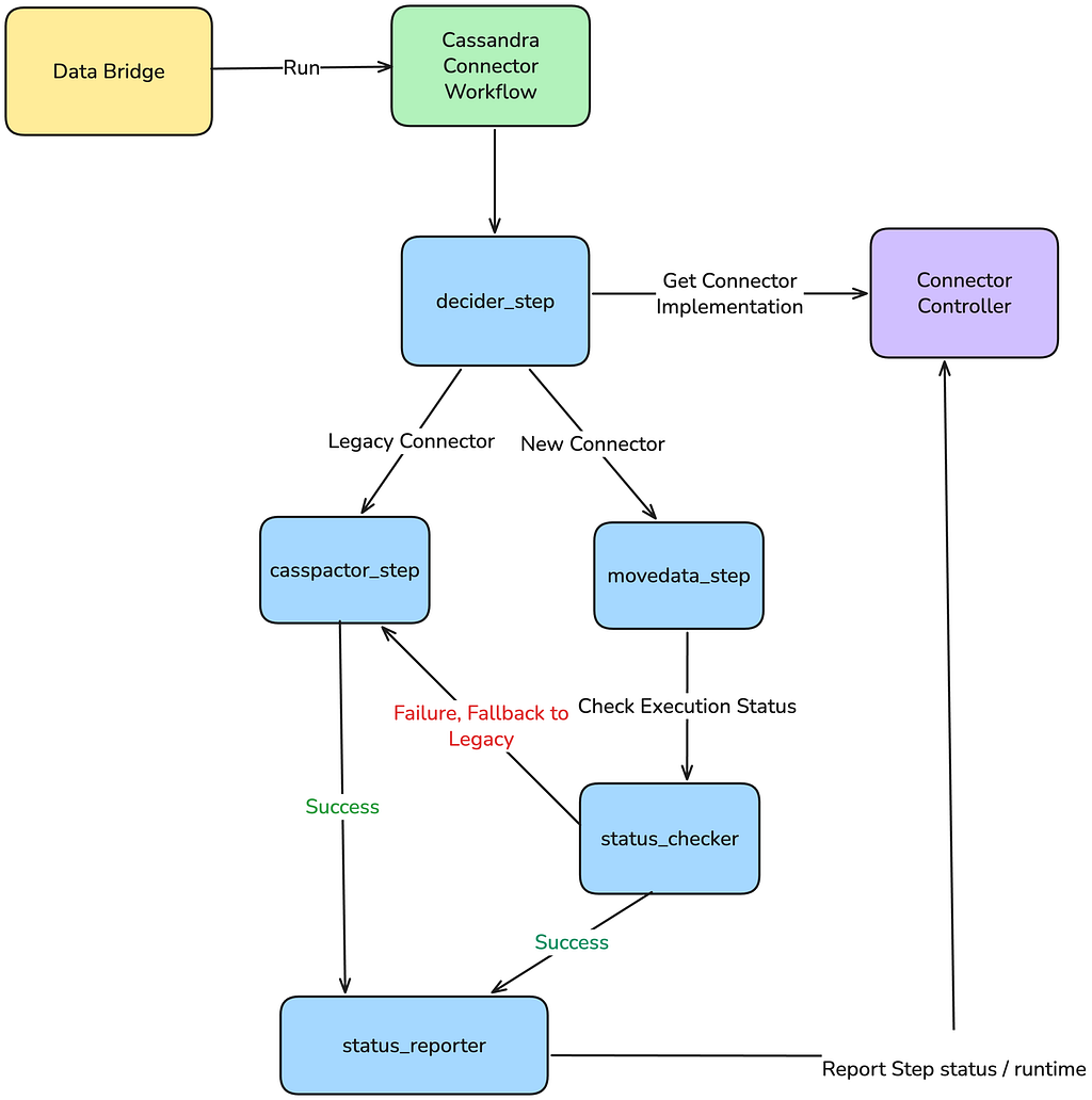
To achieve a transparent swap, we leveraged the Maestro workflow orchestration platform to implement the Decider pattern:
Data Movement Abstraction: From a user’s perspective, their Data Movement job definition remained the same.
The Decider Step: Internally the workflow responsible to execute the job was modified to include a Decider step. This step took the data movement parameters (source cluster, table name, destination) and invoked a control plane: Connector Controller.
Connector Controller as the Registry: The control plane served as the dynamic registry. Based on the migration cohort and the data movement attributes, it determined and reported the appropriate connector to use either Casspactor (legacy) or Move Data (new).
This abstraction gave our team complete control. We could upgrade or rollback any connector for any data movement instantly by simply updating a configuration in the controller, with zero modification required to the thousands of downstream customer workflows. Crucially, this abstraction guaranteed the critical safety net: a conditional step in the Maestro workflow logic ensured that if the Move Data step fails, it would immediately execute the Casspactor step.
This pattern would increase the chances that the user’s data movement completes successfully, even if the new connector encountered a bug or transient failure during the initial rollout phases. User impact was completely eliminated; they might see a slightly longer runtime in the event of a failure and fallback, but they would never see a migration failure or suffer from stale data.
Image 5: The Decider Pattern Implementation via Maestro
Beyond the workflow, the new system architecture itself was inherently more resilient. By building the new data movement connector on Cassandra Analytics and reading backups directly from S3, we removed fragile dependencies on deprecated internal services.
Conclusion
The migration from Casspactor to the new, layered architecture built on Cassandra Analytics and the Move Data connector was more than a typical “tech debt” project; it was a fundamental shift in our approach to data movement reliability and scalability at Netflix.
The legacy system, while serving us well for years, was ultimately constrained by monolithic design, fragile metadata dependencies, and an inability to handle the complexity of modern data abstractions. The new stack resolves these issues by delivering a robust, cost-efficient, and inherently more resilient solution that reads directly from S3, handles wide partitions gracefully, and eliminates costly intermediate tables.
Our blueprint for the migration, anchored by the three pillars of Validation, Visibility, and Safety, ensured a transparent and high-confidence transition. Through rigorous shadow testing and a data-driven audit framework, we achieved the desired data consistency. Enhanced dashboards and alerting provided the real-time operational insight necessary to manage risk. Most critically, the implementation of the Decider pattern within our workflow abstraction minimized the impact for all downstream users.
This successful migration validates a core philosophy: by abstracting complexity at the platform level, we can perform large system migrations without burdening our product engineering partners. The new foundation is now ready to support the next generation of Netflix’s data abstractions.
Looking ahead
This foundational work on the Cassandra Data Movement stack has done more than just replace a legacy system: it has become an accelerator for innovation across the entire Data Movement organization. By providing a reliable, performant engine that standardizes data retrieval into Spark DataFrames, we’ve enabled the rapid development of new, highly optimized connectors. This new “Connector Factory” approach has already delivered a dedicated Key-Value to Iceberg and Time Series connectors, both of which are fully aware of their respective data models, eliminating costly post-processing. This architecture is also paving the way for ambitious new initiatives, including the development of a solution for bulk loading data into Cassandra itself, effectively completing the data movement cycle, and enabling safer fleetwide connector rollout with canaries inspired by the Decider Pattern.
We are incredibly grateful for the extensive collaboration among the Data Movement, Data Bridge, Online Data Stores, Membership, Billing, Subscriber and Ads platform teams at Netflix; this work simply couldn’t have been accomplished without their partnership!
In his seminal book “Thinking, Fast and Slow,” Daniel Kahneman describes two systems that drive human cognition: System 1, which operates automatically and quickly with little effort, and System 2, which allocates attention to more challenging mental activities requiring deliberate focus. This dual-process theory has profound implications not just for understanding human behavior, but for designing intelligent systems that must balance immediate responsiveness with strategic foresight. Similar “plan vs. act” decompositions show up in other domains too — for example, robotics and autonomous driving often separate a slower planning layer (setting goals and constraints over longer horizons) from faster control and execution loops, and modern LLM agents frequently pair deliberate planning with rapid, step-by-step tool use and reaction.
At Netflix, our messaging platform faces a similar challenge every day. We send hundreds of millions of personalized notifications — push messages, emails, and in-app alerts — to help members discover content they’ll love. This creates a central tension: optimizing each notification for near-term engagement can conflict with what is best for the member over the long term. Higher message frequency can increase fatigue and opt-out risk, while lower frequency can reduce awareness of relevant titles and features the member would value.
This blog post introduces our framework for personalized notifications — a hierarchical system where a “slow” policy makes strategic, personalized decisions about a member’s weekly messaging plan (e.g., the intended frequency per channel and the resulting pacing over the week), while a “fast” policy handles the tactical, real-time decisions about which specific message to send when a send opportunity occurs. Together, they balance near-term engagement with longer-term member experience.
The Problem:
Before introducing our new framework, it is helpful to ground the discussion in a representative baseline for a personalized notification system. In our previous production system, we used a causal model to make send decisions by predicting the causal effect of a single message over a short time horizon. While this approach is effective as a baseline, it suffers from two fundamental limitations:
Short-Term Reward Horizons
The single-message outcome model is trained to optimize short-horizon metrics, such as immediate user actions occurring shortly after a notification is sent. While this is excellent for driving near-term engagement, it misses the cumulative, long-term effects of a messaging strategy. A message that drives an interaction today might also contribute to notification fatigue, reducing responsiveness in the weeks to follow. Because critical indicators of member satisfaction — like sustained viewing habits or gradual opt-out risk — only surface over extended timeframes, a short-term model will always miss the bigger picture.
Coupled Ranking and Pacing Decisions
When a single system evaluates daily incrementality to decide both whether to send something and, if so, which item to send, an individual member’s weekly message frequency becomes a by-product of those daily decisions rather than an explicit control variable. In our previous single-policy system, frequency was controlled implicitly through a relevance threshold on the model score calibrated to achieve a target aggregate send rate. While effective for managing overall frequency, this mechanism limited the system’s ability to personalize frequency based on individual engagement patterns. Moreover, because send eligibility and message selection were coupled in the same decision rule, adjusting the threshold to control frequency also changed the distribution and quality of selected messages, and vice versa.
To solve these challenges, we needed a system that could separate longer-term strategy from shorter-term decisions. What if we could determine an optimal, personalized message plan for each member, and then focus on selecting the most relevant content within those bounds? In the following sections, we detail how we realized this vision by decoupling our notification engine into a hierarchical ‘System 1’ and ‘System 2’ framework.
The Proposed Method: A Hierarchical Slow-Fast Architecture
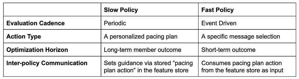
The Slow policy’s primary role is to define a personalized pacing of messages over a defined time horizon. The decisions made by slow policy are consumed by the Fast Policy whose role is to maximize immediate relevance and select the optimal message for the member at any given moment.
To illustrate the Slow Policy in practice: For example, if optimized at a weekly cadence, the policy evaluates a member’s long-term engagement patterns to select a “Pacing Plan Action.” To keep the action space manageable yet expressive, we discretize the decision space into a set of actions that independently specify push and email frequencies. This provides approximately O(100) distinct combinations of cross-channel pacing strategies.
The Utility Function
The Slow policy selects actions by maximizing a personalized utility function. This function explicitly trades off positive engagement signals against the long-term “cost” of messaging.
To capture a holistic view of member health, this utility is composed of:
Positive Signals: Capturing the likelihood that a member will find value in and engage with the platform.
Negative Signals: Capturing the likelihood of member fatigue or a propensity to opt out of a messaging channel.
Ideally, negative signals alone would naturally penalize over-messaging. In practice, however, explicit negative feedback is extremely sparse. Without an additional constraint, the predicted ‘cost’ of an incremental message appears negligible, causing the model to gravitate toward maximum frequency.
To address this, we introduce a universal message cost that is added to the personalized negative‑feedback prediction for every send. This additional cost term keeps the reward function concave and well‑behaved, preventing degenerate “always send” policies. The message cost parameter is empirically tuned using a combination of online experiments and offline evaluation metrics.
Pacing Strategy
The two-stage design naturally allows for optimizing both the average frequency as well as pacing of messages over time. The simplest pacing strategy is uniform random: we translate the frequency target into a per-opportunity send probability and, at each eligible opportunity, effectively flip a weighted coin to decide whether to send. This produces an organically randomized pattern whose expected send rate matches the target.
While uniform pacing provides a clean and robust baseline, the framework readily extends to richer, non-uniform pacing profiles (for example, day-of-week patterns, conditioning on user activity, or launch-aligned bursts) whenever product or user-experience considerations call for more structured temporal distributions.
Policy-to-Policy Communication
The true power of this hierarchy lies in decoupling. By splitting into “Slow” and “Fast” policies, we allow each to focus on what it does best.
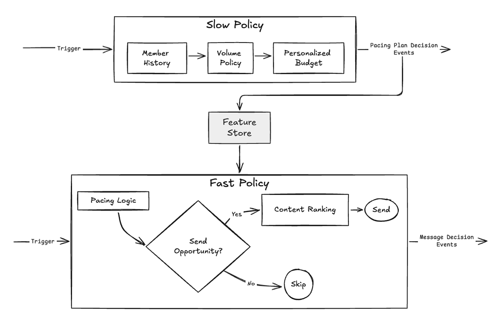
To bridge these two worlds asynchronously, decisions are events and state is managed through a low-latency feature store:
The Planner (Slow): The Slow policy calculates a member’s ideal pacing plan. It writes this strategic intent to a feature store
The Executor (Fast): Every day, when a notification opportunity arises, the Fast Policy simply pulls that stored “plan” as a feature. It then executes the tactical send decision within those strategic guardrails.
This architecture provides two critical advantages:
“Stickiness”: It ensures a member receives a consistent experience. The Slow policy will be executed once at a defined cadence; the plan is stored and honored.
Independent Evolution: We can retrain, optimize, or A/B test our weekly pacing strategies (the “Slow” layer) without ever touching the real-time ranking logic (the “Fast” layer).
Figure 1: Schematic of the two-layer message personalization system composed of a slow planning policy (top) and a fast execution policy (bottom). A feature store serves as the communication bridge between the two policies.
Key Results & Takeaways
The transition to a hierarchical architecture resulted in one of our largest production metric lifts to date. We observed several key breakthroughs:
Empowering the “Casual Viewer”: Gains were most significant among members who watch less frequently — a critical cohort where timely, high-relevance awareness of new content is vital.
The Power of Decoupling: Separating frequency planning from message selection was as transformative as the modeling itself. This new architecture unlocks incredible flexibility, allowing us to iterate on content ranking models and pacing strategies as two independent, clean variables.
Respecting the Horizon: The impact of messaging is rarely an isolated event; its effects build up cumulatively based on ongoing interactions between our system and the member. By isolating pacing into a dedicated strategic layer, we now have the mechanism to explicitly manage long-term fatigue and opt-out risk.
Acknowledgments
We could not have delivered this project without the help of our outstanding colleagues, and we sincerely thank them for their contributions.
By Winston Chou, Adrien Alexandre, Lars Olds, Yi Zhang, Garrett Hagemann, and Nathan Kallus
Introduction
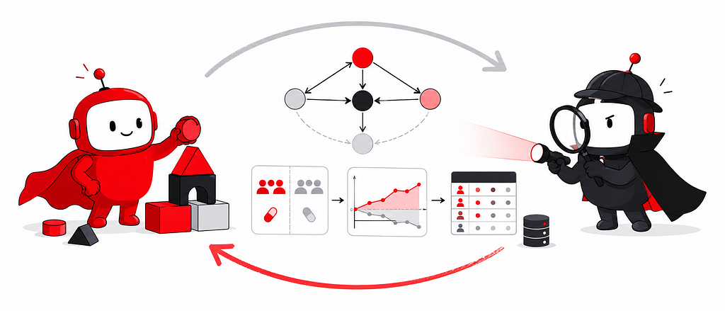
Imagine asking a data agent to analyze the causal relationship between two variables, such as the effect of watching a popular Netflix show on long-term member retention. It queries your data, runs a regression, and confidently returns an answer. How much should you trust it? Can you be confident that the agent accounted for subtle biases — or does it treat passionate fans as if they were the average viewer? Without deep understanding and expertise, would you even be able to tell if it got the answer wrong?
Data analysis is increasingly being delegated to software agents. While this reduces human effort and toil, oversight is still needed to ensure the validity of results. This is especially true for specialized tasks like Observational Causal Inference (OCI), which require substantial judgment and domain expertise.
In this blog post, we share an agentic workflow for performing OCI under unconfoundedness. Our workflow is designed for software agents to adhere to rigorous, exhaustive templates for causal inference tasks. Yet, it also seeks to be “human-augmenting,” and to enable and empower human inspection and evaluation.
We designed this workflow with OCI practitioners in mind. Although OCI requires context and care to do well, aspects of it — e.g., checking and rechecking covariate balance, conducting sensitivity analyses, and keeping track of multiple iterations — can be repetitive and prone to error. Our workflow seeks to eliminate this toil so that humans can focus on more nuanced tasks, such as framing questions, scrutinizing assumptions, and evaluating results.
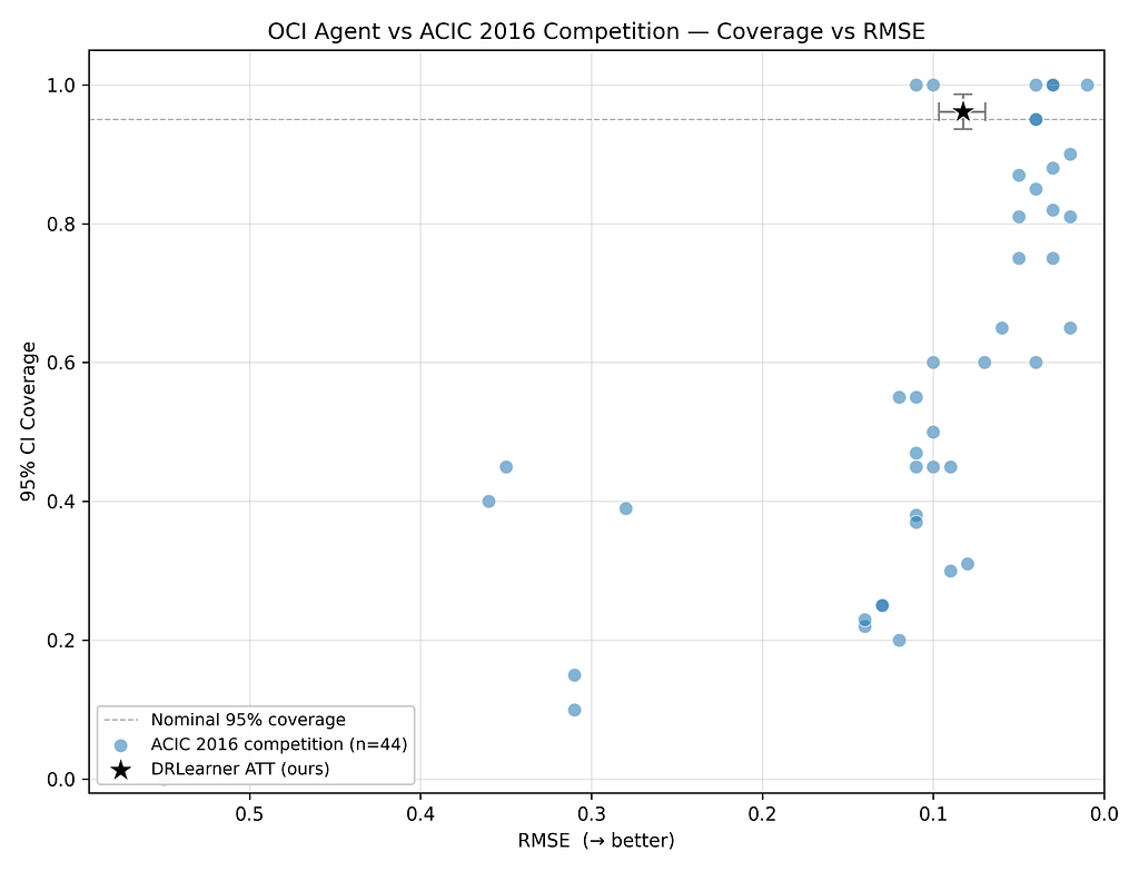
To this end, we are open-sourcing a standalone version of our oci-agent so that OCI practitioners can model workflows on and suggest improvements to it. We also share evaluations of our agent on the 2016 Atlantic Causal Inference Conference (ACIC) competition datasets, and show that our agent systematically beats one-shot iterations under numerous data-generating processes — while achieving competitive results against hand-tuned benchmarks.
This post describes the principles behind our workflow and gives a case study of its deployment at Netflix.
Philosophy
Our workflow is built on top of Netflix’s pre-existing OCI toolkit. We built this toolkit — largely in a pre-AI world — to answer “point-in-time” causal questions, such as “what is the effect of playing a Netflix game on member retention?” or “what is the effect of watching a highly popular show on subsequent engagement?” Questions of this kind inform business strategy, guide metric development, and contribute to a rich understanding of what drives member satisfaction.
Our toolkit is guided by a “target trial emulation” philosophy. For any point-in-time OCI question, we ask “what is the ideal A/B test for addressing this question?” This A/B test may be expensive, slow, or even infeasible to run. However, the thought exercise helps to pin down the assumptions needed for a credible answer, such as unconfoundedness of the treatment.
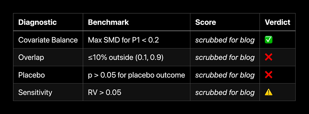
To make the target trial analogy actionable, our toolkit embeds a series of design diagnostics. These diagnostics assess whether we are drawing fair comparisons between treated and untreated units — or if there are hidden differences that could imperil our conclusions:
Covariate balance. After weighting, the standardized mean difference of pre-treatment covariates between treatment and control groups should be less than 0.2.
Overlap. The probability of receiving treatment (aka propensity score) should be bounded between 0.1 and 0.9.
Placebo outcome. The “treatment effect” on variables measured prior to the treatment should not be significantly different from zero.
Sensitivity to hidden confounders. Findings of treatment effects are contextualized by sensitivity to hypothetical omitted variables that explain both treatment and outcome.
As we uplevel our OCI toolkit with agents, such evaluation remains paramount. The standard approach to evaluating agents is to programmatically compare their outputs to ground truth. Yet, outside of artificially simulated data, there is no ground truth in observational causal inference.
Without discounting the need for evals (which our workflow also supports), one of our key principles is to augment human evaluation by making each analytic step as transparent as possible. For example, in our workflow, agents publish artifacts in the form of plans, specifications, plots, and notebooks that humans can inspect and re-execute if they wish. In the absence of ground truth, we rely on these “process audits” — coupled with human oversight — to build good agents.
Principles
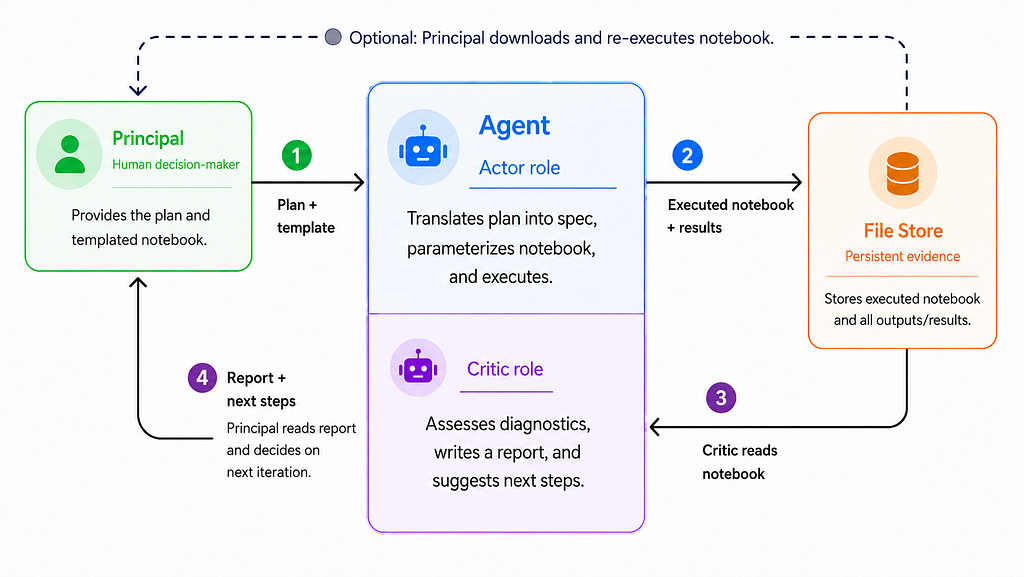
Our workflow has three key personas:
Principal — the human user (e.g., data scientist) whose goal is to provide a thorough and correct analysis
Actor — the software persona that performs the analysis, including diagnostics
Critic — the software persona that synthesizes results, identifies gaps, and offers suggestions to improve the analysis
Our agent orchestrates the latter two personas in an actor-critic loop: specifying and triggering the analysis as the actor, then interpreting results and diagnosing flaws as the critic.
Each persona has responsibilities:
Principals
Provide an initial analysis plan containing its context and goals.
Provide context on the main threats to valid inference and the confounders that must be controlled.
Specify the tools that can be used for the analysis.
Specify the data model and dataset.
Actors
Refine the principal’s plan into a data analysis spec.
Use only the tools provided by the principal.
Create human- and machine-checkable artifacts.
Perform the four design diagnostics in addition to the core analysis.
Report any remediations taken in case of diagnostic failures.
Critics
Check for blind spots, such as unmentioned confounders, in the principal’s plan.
Check for alignment between the plan, spec, and executed analysis.
Specify a credibility level in the results after seeing the diagnostics.
Specify if and how the estimand differs from the Average Treatment Effect (ATE), for example due to propensity score trimming.
Contrast the executed analysis with the ideal target Randomized Controlled Trial (RCT).
Suggest at least one alternative measurement strategy (e.g., encouragement RCTs).
Although our workflow is designed for OCI under unconfoundedness, the principles listed in this section are meant to be extensible to other approaches to OCI, such as panel methods with very different assumptions (e.g., parallel trends).
Empowering Human Evaluation
To empower human oversight of each analytic step, we provide principals with a templated notebook that uses our vetted (non-agentic) OCI toolkit, which employs doubly robust learning for causal effect estimation.
The principal’s remaining responsibilities are to write the initial analysis plan and to evaluate the analysis artifacts (the executed notebook and the critic’s report). To enable thorough evaluation, agents version-control their reports and upload executed notebooks to a file store, where they can be downloaded and re-executed by principals (if they wish).
We diagram this workflow below:
Case Study — Estimating the Impact of New Entertainment Types
In recent years, we have added a wide variety of entertainment types beyond streaming video to Netflix. A natural question is how these new entertainment types affect members’ satisfaction and their likelihood of continuing to subscribe to Netflix.
To analyze the impact of one of these new entertainment types, which we will call Type X, we wrote a simple analysis plan specifying our
Treatment: Days engaging with Type X (or “Type X days” for short)
Outcome: Two-month retention
Potentialconfounders, including pre-treatment Type X days
To establish a baseline, we fed this analysis plan without additional scaffolding to Claude Sonnet 4.6, a powerful yet accessible general-purpose model. The model chose and executed a defensible analysis strategy: linearly regressing retention on Type X days along with controls.
While the result was polished and impressive, when we ran the same analysis through our paved path tooling and agentic workflow, also using Sonnet 4.6, our agent produced an updated estimate that was just 25% of the baseline! What explains the difference between the baseline and the paved-path estimates?
A core challenge when analyzing new entertainment types is early adopter bias. The first users of any new offering are likely to be systematically different from the general population. For example, they may be heavier users of Netflix generally, or they may be extremely strong fans of the underlying titles. Early adopter bias manifested in our analysis as poor “overlap”: the vast majority of observations had a small estimated probability of engaging with Type X, reflecting its early maturity.
This imbalance was caught by our critic agent in its writeup of the analysis. The critic also flagged the failure of the placebo test: early Type X adopters differed significantly from non-adopters in terms of important confounders measured before experiencing the treatment, a warning sign of potential bias.
Addressing Failed Diagnostics
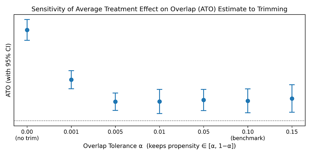
To address these diagnostic failures, our workflow provides agents with a playbook. For example, to overcome poor overlap, we instruct the agent to use Crump-style trimming. That is, before estimating causal effects, the actor trims units with estimated propensity scores outside the range [0.1, 0.9]. This scopes the treatment effect being estimated to the ATE in the population that is not very likely or unlikely to engage in the new entertainment type — an important caveat we instruct the critic to flag in its report.
Trimming yields an estimate that is much smaller than the baseline estimate, and which only applies to the “overlapping” population (for whom engagement with the new entertainment type is non-deterministic). However, the trimmed estimate is substantially more credible, as it focuses on the members for whom the treatment could plausibly be randomly assigned, as in a target trial.
Contrastively, the baseline effect relies heavily on assumptions to extrapolate outcomes for all members, even those with a very low probability of treatment. The danger here is that extrapolation produces a number that is not backed by robust data and is likely confounded by early adopter bias.
Orchestrating Followup Analyses
There are two natural followups to this analysis:
First, we need to analyze the sensitivity of estimates to the choice of trimming threshold. Practically, this requires redoing the analysis with multiple trimming thresholds.
Second, we also care about how these causal effects evolve over time. Yet, comparing causal effects across time raises subtle challenges. For example, we need to coordinate the population across all analyses: if a set of users is trimmed to make one analysis more credible, it should be trimmed in the other analyses as well.
Both of these followups require conducting multiple versions of the same analysis, tweaking some parameters while keeping others the same. Managing this complexity and ensuring consistent execution is another area where agents add value.
To illustrate this, below we show a sensitivity analysis for our case study in which we asked the agent to vary the trimming bounds from [0, 1] (no trimming) to [0.15, 0.85]. As the plot shows, the estimated ATE on the overlapping population is robust to the choice of trimming threshold within bounds of [0.005, 0.995]. Although principals could (and should) execute this and other robustness analyses, delegating them to agents helps to reduce toil.
Another example is generating a time series by repeating the same analysis across multiple date partitions. For example, below we plot the results of using our agent to refit a different analysis on ten distinct date partitions. The plot shows evidence of seasonality: the treatment has a stronger effect on the winter dates compared to the summer dates.
Public Repo and Evals
To help OCI practitioners build on and contribute to our workflow, we are open-sourcing a standalone version of oci-agent. This repo implements two evaluations on public datasets from the 2016 Atlantic Causal Inference Competition (ACIC) data analysis competition. It also includes a lightweight version of our internal causal machine learning notebook that only uses open-source software (EconML).
Our first evaluation runs this notebook for three randomly sampled datasets generated by each of the 77 data-generating processes (DGPs) in the ACIC data. Next, it uses the critic to grade the resulting 231 estimates as either satisfactory or unsatisfactory based on the diagnostics.
Below, we plot the average RMSE and coverage of 95% confidence intervals of our ATT estimates against the 44 competitor methods in the ACIC competition. As the scatterplot shows, our statistical methodology is competitive against these benchmarks: it achieves reasonably low RMSE and well-calibrated confidence intervals that cover the truth in ~95% of DGPs.
More to the point, our diagnostics and agentic workflow help to separate more reliable estimates from less reliable estimates. To illustrate this, the following chart plots our ATE estimates in terms of RMSE and coverage. Note that we separate out the RMSE and coverage of:
All 231 estimates (purple dot)
The 192 satisfactory estimates (blue star)
The 39 unsatisfactory estimates (red dot)
As the plot shows, when aided by our diagnostic suite, the critic agent is able to separate good estimates from bad estimates: the satisfactory estimates have much lower RMSE and better calibrated confidence intervals than do the unsatisfactory estimates.
Our second evaluation compares the performance of an LLM on the same analysis plan with our scaffolding and without it (i.e., one-shot prompting). Unsurprisingly, we find that our scaffolding is critical to helping the LLM return useful estimates. This can be seen in the following random sample of ten ACIC datasets. Using our scaffolding, the LLM recovers the ground truth in nine out of ten datasets. Furthermore, estimates are highly correlated with ground truth.
In contrast, giving the same analysis plan to Sonnet 4.6 without any scaffolding (i.e., just prompting it) results in consistently wrong answers that are not at all correlated with ground truth.
A key limitation of our public repo is that, due to the synthetic nature of the underlying datasets, it doesn’t pressure-test our agent’s semantic understanding or performance on real-world OCI tasks. Nonetheless, the repo demonstrates the core principles underlying our workflow. These include (1) giving agents with extensive scaffolding so that they follow best practices by design, and (2) requiring inspectable artifacts so that humans can audit agents’ processes, not just their outcomes.
Conclusion
We provide a workflow for doing observational causal inference with the help of software agents. Leveraging elements of our pre-AI OCI toolkit, such as templated notebooks, our workflow is designed to ensure that agents conduct rigorous and exhaustive analyses. This helps to reduce the human toil of OCI, which can be a highly iterative and exacting process.
At the same time, motivated by the complexity and ambiguity of observational causal inference, our workflow seeks to be human-augmenting and enables human practitioners to evaluate each analytic step.
Using agents for causal inference poses a challenge: how do we evaluate agents’ performance on tasks without ground truth? To meet this challenge, our workflow combines process audits with human oversight. To enable others to learn from and critique our workflow, we have open-sourced a lightweight, standalone version. We hope this work stimulates more research and development on agentic evaluation in the absence of ground truth.
For valuable feedback on this post and “dogfooding,” we thank Adith Swaminathan, Ayal Chen-Zion, Colin Gray, Juliet Hougland, and Simon Ejdemyr.
Will this encode look good to Netflix members? Does switching to a new codec improve quality at the same bitrate and by how much? What is the best way to encode a movie title given a target bitrate budget? For years, VMAF has reliably helped us answer those questions and deliver an optimized quality of experience to our members.
But good is not good enough. If VMAF misjudges quality, that may lead to loss of detail for a suspenseful close-up or banding for a stunning wide-angle sky shot. That’s a lot of trust to put in one number, so we strive to make sure it earns it. Over time, we collected feedback from VMAF users, both internally and externally. A few years ago, we embarked on a journey to develop a new version of VMAF to address some of its known limitations. Today, we are happy to announce that we are open-sourcing a new version of VMAF, with version number v1. By using VMAF v1 we can more accurately assess visual quality and hence efficiently deliver higher quality for Netflix members worldwide. In this post we share how v1 addresses the previous version’s (called VMAF v0) limitations and some of the challenges we faced along the way.
What is VMAF and why improve it?
VMAF (Video Multimethod Assessment Fusion) is a video quality metric that Netflix developed with university partners and open-sourced on GitHub. It has become a de facto standard for encoding evaluation and optimization for the video industry. VMAF combines elementary quality-aware features and fuses them with a support-vector regressor (SVR) trained on subjective data. For background, see our first, second and third VMAF tech blogs.
Despite its accuracy and wide adoption, we have identified room to improve the core of the algorithm. That’s central to our mission of delivering the best possible visual quality to our members no matter where and how they watch Netflix. As new codecs, like AV2, are developed and use cases like live streaming and cloud gaming emerge, we strive to continue to improve VMAF to serve these business needs. We describe each key improvement below.
Improving sensitivity to compression artifacts
As discussed in our first VMAF tech blog [1], a typical encoding pipeline introduces both compression and scaling artifacts. Intuitively, when more bits are available, higher resolutions are preferable. VMAF quantifies the tradeoff between compression and scaling and determines the optimal resolution to use given a bitrate budget. This can be demonstrated by a VMAF vs. bitrate curve.
In practice, we observed that VMAF v0 tends to favor switching to a higher resolution at lower bitrates, preferring compression artifacts over scaling, which could be visually annoying. This can be partially attributed to the DLM (Detail Loss Metric) feature, which penalizes contrast/detail loss, but may be less sensitive to distracting artifacts, like blockiness [3]. In VMAF v1, to complement DLM, we added the AIM (additive impairments) component [3] from the original ADM formulation with minor modifications to improve accuracy. These two elementary metrics are linearly combined, similar to the original implementation in [3].
One VMAF model to rule them all
A first-order effect that influences quality perception is the visibility of artifacts and its relationship to viewing distance and canvas size. Put simply, the same encoded video looks better when displayed on a smaller canvas or viewed from further away.
The standard VMAF model assumes that viewers sit in front of a 1920×1080 display, in a living room-like environment, with a normalized viewing distance of approximately 3× the screen height (3H). This means that the standard 1080p@3H VMAF model corresponds to a viewing angle of approximately 60 pixels per degree.
For phone viewing, given a smaller screen size and longer natural viewing distance (typical phone viewing can be approximated as 4 to 5H) relative to the screen height, we expect that artifacts become less visible. The phone model of VMAF v0 captures this by post-processing the standard (TV/laptop) VMAF score by a second-order polynomial mapping. This mapping was estimated using subjective data.
One drawback of the above mapping is that it is hard to generalize predictions for the myriad of viewing conditions that materially differ from the original subjective experiment. Further, in practice, we observed that the phone model can overpredict quality. In v1, instead of using a mapping function, we adjust the elementary feature values based on the normalized viewing distance. The same model can then be trained and reapplied for different use cases, e.g., phone viewing, 4K@3H, or a more discerning [email protected]. We found that this approach improves accuracy and helps generalize VMAF better.
To achieve this, we modulate the spatial contrast sensitivity function (CSF) used in DLM based on the normalized viewing distance. The CSF defines human sensitivity to contrast across spatial frequencies and is related to distortion perceptibility. The CSF can hence be used to estimate perceived distortion for different viewing distances, display sizes, and resolutions. An example CSF curve is shown below.
As the viewing distance increases, more pixels fit into a degree of visual angle, which lowers distortion visibility. In VMAF v1, we use an adapted version of Barten’s CSF model from [4].
Addressing banding artifacts
Banding shows up as staircase-like edges in parts of the image that should look smooth. It can have a negative visual impact for viewers, but this impact is not captured well by VMAF v0. VMAF v1 integrates the Contrast Aware Multiscale Banding Index (CAMBI) as one of the elementary features. You can read more about CAMBI in our previous tech blog or the technical paper.
Addressing chroma artifacts
VMAF v0 only extracts luma-based features, so it is unaware of chroma artifacts. In practice, encoding and scaling introduce chroma artifacts via quantization and subsampling. To capture such artifacts, we modified SpEED-QA and applied it to the chroma channels.
Leveraging the no-enhancement gain (NEG) mode
To reduce the effect of image enhancement operations, like sharpening, a standalone no-enhancement gain (NEG) mode was made available for VMAF v0. We have found that NEG serves as a conservative quality metric and helps preserve creative intent. We already use VMAF-NEG as one of the quality metrics during codec development, such as for AV2. Therefore, NEG is enabled by default for VMAF v1 without a need for a separate model.
Improving the motion feature
VMAF v0’s motion feature does not have an upper bound. Further, the training data used then did not have enough coverage for high-motion sequences. Consequently, we observed that VMAF v0 could overpredict quality for very high-motion scenes. On the flip side, since motion differencing in v0 was performed between consecutive frames, v0 would underpredict quality for sequences with frame rates higher than 24 or 30 fps, like 60 fps. In v1, we apply an empirically derived hard threshold to the motion feature. Further, we add an option to measure motion differences over a larger temporal window. Expanding the temporal window alone does not fully capture the perceptual impact of 60 fps, but it does reduce the underprediction evident in v0.
Overview of VMAF v1 models
VMAF v1 supports the following models:
Standard 1080p Model: This model is calibrated for 1080p video viewed at a standard 3H distance. It uses an operating range of [0, 100].
Phone Model: Derived by setting the normalized viewing distance to 5H (based on experimental data), this model adjusts the DLM, AIM, and chroma feature calculations to reflect reduced artifact visibility on smaller screens viewed from a greater relative distance. It retains the standard [0, 100] range.
4K Model: We release two v1 4K models: a 1.5H variant and a 3H variant. The 1.5H variant is based on a discerning [email protected] viewing condition. This variant is conceptually similar to its v0 4K counterpart and operates on a [0, 100] range. For most users, this variant is the default choice. The 3H variant is based on a consumer-like 4K@3H viewing condition. This variant operates on a [0, 110] range, which helps to quantify the additional perceptual benefit of 4K resolution over 1080p when both are viewed at 3H.
Interpreting the score
VMAF v1’s score and interpretation are largely consistent with v0’s. To achieve this, we calibrated the VMAF v1 scale to align with v0 via a score transform, so that the new algorithm preserves the meaning of the numbers while keeping its accuracy benefits.
Putting v1 to the test
We evaluate VMAF v1 across several subjective datasets. These datasets cover a variety of codecs, content types, and use cases. For simplicity, we report the Spearman’s rank correlation coefficient (SRCC) for VMAF v0 and v1. SRCC values closer to 1 show higher agreement with subjective data. Full results will be available in a future technical paper.
In the table below, if a dataset is marked as “4K” then we measure VMAF at 4K using the [email protected] model, otherwise we measure VMAF at 1080p, using the appropriate 1080p model. If a dataset is marked as “phone” the 1080p phone model is used, otherwise the standard 1080p@3H model is used.
NFLX Banding + compression: Contains 83 AV1 videos encoded at different bitrates under banding-relevant conditions. NFLX How Low Phone: Contains 80 AVC videos encoded at 540p and below to understand viewer acceptability to low qualities. “train-only”: only the training split was publicly available.
As seen above, VMAF v1 matches or outperforms v0 in most datasets. There are notable improvements on large datasets like WATERLOO IVC 4K and the Netflix Screen Size Crowdsourcing, on datasets with chroma and banding artifacts, and those that involve phone viewing. On a few datasets we observe minor regressions, which are small relative to the gains elsewhere.
Running v1
Even with the addition of new features, we wanted VMAF v1 to have a reduced computational complexity when compared with VMAF v0. To achieve this, we have:
Removed VIF (Visual Information Fidelity) as a core VMAF feature. VIF is computationally complex and did not meaningfully improve accuracy after updating the other features.
Introduced a few CAMBI-specific optimizations, both algorithmic and software.
Measured the chroma feature at a lower scale, which does not hurt accuracy [11].
The result of this work is not only a more accurate VMAF, but also a much faster VMAF. The table below shows the processing speed and threading performance for each VMAF model at 1080p and 4K. Additionally, our newest libvmaf release has a much improved threading performance, which is of benefit to both v0 and v1. Note that for content with significant banding, computing CAMBI adds some overhead, which can reduce this speedup.
While the core of the algorithm has changed, we still recommend:
Computing VMAF at the right resolution by upsampling the distorted video to the source resolution, so that both compression and scaling artifacts are reflected. For example, bicubic upsampling can be used as a general approximation.
Interpreting scores in context by using the right model (e.g. 1080p vs. 4K vs. phone) for your scenario by taking into account viewing distance assumptions.
This is not the end of the road
Just like any metric, VMAF v1 is not perfect. There is still room for improvement. Some areas that we are working on addressing in the future are: film-grain noise, improved handling for high frame rates, and perceptual codec optimizations such as adaptive quantization. We invite the community to try the latest VMAF models, report edge cases, contribute to the open-source code, and help improve VMAF. We plan to publish a detailed technical paper for VMAF v1. We also plan to release an HDR version enhanced by the v1 improvements, so stay tuned!
Acknowledgments
This was a collaborative effort propelled by our stunning colleagues. We want to thank the following individuals: Xiaoqing Zhu, Mariana Afonso, Anush Moorthy, Raymond Walsh, Omair Akhtar, Amelia Taylor, Ken Thomas, Zheng Lu, Chris Pham, Alex Chang, Prudhvi Chaganti, Ben Wallen, Craig Howland, Deepthi Arun, Andy Rhines and Lukáš Krasula.
[3] S. Li, F. Zhang, L. Ma, and K. Ngan, “Image Quality Assessment by Separately Evaluating Detail Losses and Additive Impairments,” IEEE Transactions on Multimedia, 2011.
[4] P. G. J. Barten, Contrast Sensitivity of the Human Eye and Its Effects on Image Quality. SPIE Press, 1999.
[5] Video Quality Experts Group, “Report on the validation of video quality models for high definition video content,” 2010.
[6] N. Barman, Y. Reznik, and M. G. Martini, “A Subjective Dataset for Multi-Screen Video Streaming Applications,” International Conference on Quality of Multimedia Experience (QoMEX), Ghent, Belgium, 2023, pp. 270–275.
[7] A. Katsenou, F. Zhang, M. Afonso, G. Dimitrov, and D. R. Bull, “BVI-CC: A Dataset for Research on Video Compression and Quality Assessment,” Frontiers in Signal Processing, vol. 2, 2022.
[8] C. G. Bampis, L. Krasula, Z. Li, and O. Akhtar, “Measuring and Predicting Perceptions of Video Quality Across Screen Sizes with Crowdsourcing,” International Conference on Quality of Multimedia Experience (QoMEX), Ghent, Belgium, 2023, pp. 13–18.
[9] J. Y. Lin, R. Song, C.-H. Wu, T. J. Liu, H. Wang, and C.-C. J. Kuo, “MCL-V: A streaming video quality assessment database,” Journal of Visual Communication and Image Representation, vol. 30, pp. 1–9, Jul. 2015.
[10] Z. Li, Z. Duanmu, W. Liu, and Z. Wang, “AVC, HEVC, VP9, AVS2 or AV1? — A Comparative Study of State-of-the-Art Video Encoders on 4K Videos,” Int. Conf. Image Analysis and Recognition (ICIAR), 2019.
[11] C. G. Bampis, P. Gupta, R. Soundararajan, and A. C. Bovik, “SpEED-QA: Spatial Efficient Entropic Differencing for Image and Video Quality,” IEEE Signal Process. Lett., vol. 24, no. 9, pp. 1333–1337, Sep. 2017.
[12] L.-H. Chen, C. G. Bampis, Z. Li, J. Sole, and A. C. Bovik, “Perceptual video quality prediction emphasizing chroma distortions,” IEEE Trans. Image Process., vol. 30, pp. 1941–1954, 2021.
Organizations that use feature flags alongside incident response tooling often connect the two manually. When an outage occurs, engineers must identify which flags are relevant, decide whether to disable them, and coordinate the change across teams. This manual process adds latency at the moment it matters most.
You can use AWS DevOps Agent and its MCP server feature to connect to LaunchDarkly’shosted MCP server, enabling feature flag recommendations during both proactive deployment review and reactive incident response workflows. Once connected, DevOps Agent can query flag state, read targeting rules, and surface recommendations directly within the workflows where engineers make decisions.
This post walks through two primary use cases:
Pre-deployment review where the release management capabilities in AWS DevOps Agent evaluate changes and a DevOps Agent Skill recommends feature flag coverage before code ships.
Incident response where DevOps Agent queries LaunchDarkly flag state via MCP and recommends containment actions during active incidents.
We also cover the connection architecture, a reusable DevOps Agent Skill for pre-deployment flag validation, and links to get started.
Defense: Release Management and Proactive Flag Recommendations
Figure 1: DevOps Agent’s readiness review identifies high-risk PRs and recommends LaunchDarkly feature flag coverage before code ships.
The release management capabilities (now in public preview) in AWS DevOps Agent evaluate code changes before they ship to production.
It performs functional testing in an AWS-managed verification environment, assesses risks to cross-codebase dependencies, evaluates adherence to your organization’s standards and best practices, and mathematically verifies that access control configurations in CloudFormation do not deviate from Well-Architected best practices.
AWS DevOps Agent is designed to be extended and customized to fit your tools, standards, and practices. Using the product’s primitives, you can add Skills that enhance its capabilities. For example, when a high-risk change is identified, a custom Skill can evaluate whether the change has adequate feature flag coverage, operating on deployment metadata and code analysis to identify gaps and surface a recommendation to the developer, such as recommending feature flags with LaunchDarkly when needed.
What the Skill Evaluates
The release readiness flag Skill classifies code changes into risk tiers (Critical, High, Moderate) based on what’s being modified — payments, authentication, database schemas, third-party integrations, new API endpoints, performance-sensitive paths, and more — and recommends feature flags proportional to the risk level.
Figure 2: The high-risk-feature-flag-recommendations Skill configured in AWS DevOps Agent’s Knowledge panel.
What the Recommendation Includes
When the Skill identifies a gap, it surfaces a recommendation containing:
Risk context: Why the change is flagged as high-risk (e.g., “This deployment modifies payment authorization logic across 3 downstream services with no existing rollback mechanism.”)
Suggested flag configuration: A proposed LaunchDarkly flag key, variations, and default targeting rules aligned with the deployment plan.
Rollout strategy: A recommended phased rollout (e.g., internal users first, then 5% of traffic, then full rollout) that matches the risk profile.
Kill-switch behavior: What happens when the flag is turned off — the fallback code path, cleanup considerations, and data consistency implications.
Example Scenario
Consider a team deploying an update to a tax calculation service. The change modifies the tax rate computation logic, affecting all order totals across multiple regions. AWS DevOps Agent evaluates the deployment and classifies it as high-risk. The pre-deployment flag gate Skill then identifies:
The change touches critical-path tax calculation code.
No feature flag wraps the new computation behavior.
The blast radius covers all active checkout sessions.
The Skill surfaces a recommendation: “This deployment modifies tax calculation logic with no existing feature flag coverage. Recommend wrapping the new tax computation in a LaunchDarkly flag (tax-calculation-v2) with a phased rollout targeting internal test accounts first, followed by 5% of production traffic.”
The developer can then action the recommendation, creating the flag in LaunchDarkly, adjusting the suggested configuration to fit their rollout plan, or noting the justification for proceeding without one as part of the deployment record.
Figure 3: AWS DevOps Agent release management report identifying checkout pricing changes deployed without LaunchDarkly feature flag coverage, including a suggested fix with sample code.
Closing the Loop with Kiro IDE
DevOps Agent’s release management capabilities identify when a deployment needs feature flag coverage. Paired with Kiro IDE, this recommendation becomes actionable without leaving the development workflow.
Kiro connects to LaunchDarkly’s MCP server directly, providing flag integration capabilities during development. When a developer builds a new feature in Kiro, the IDE can query LaunchDarkly via MCP to check whether a flag already exists for that feature and generate code with the flag evaluation built in from the start.
Together, this creates one continuous flow: DevOps Agent identifies the risk and recommends flag coverage → the developer, working in Kiro, generates the flag and wraps the code in a single action → the deployment ships with coverage already in place. No context-switching between tools, no manual flag creation in a separate console.
Developers can also use Kiro’s flag integration independently during feature development, even before a deployment triggers a release management review. The two operate as layered coverage: if Kiro catches it during development, DevOps Agent validates the targeting rules match the rollout plan at deployment time. If the developer bypasses Kiro or uses a different toolchain, DevOps Agent still identifies the gap.
Offense: Flag Recommendations During Incident Response
During an active incident, speed of containment directly affects customer impact. DevOps Agent participates in incident response workflows by querying LaunchDarkly to understand current flag state, then recommending containment actions based on what it finds.
Figure 4: DevOps Agent identifies a flag change (30ms from 2000ms) as the probable cause, queries LaunchDarkly for state, and recommends reverting the value.
When you detect an incident, DevOps Agent correlates the affected service with recent deployments. It queries LaunchDarkly to identify feature flags associated with those deployments and their current state (enabled, targeting rules, rollout percentage). If a relevant flag is enabled, the agent recommends disabling it as a containment option before suggesting a full rollback.
Flag-based containment provides an alternative containment option that can help reduce the time to resolution. Disabling a flag may return behavior to the previous state, which can be faster than a full deployment rollback in some scenarios
Example Scenario
An alert fires indicating sustained 5XX errors on the bot-service. The on-call engineer engages DevOps Agent, which:
Correlates the HTTP 503 errors with a LaunchDarkly feature flag change: bot-mutation-orchestration-timeout-ms was changed from the default 2000ms to 30ms (the “low latency” variation), applied to all traffic.
Identifies that the 30ms timeout budget is insufficient for inter-service HTTP calls during bot creation and deletion orchestration, which require DynamoDB reads/writes plus IoT Core calls, causing ReadTimeout exceptions.
Recommends reverting the bot-mutation-orchestration-timeout-ms flag to its default variation (2000ms) as the containment action, noting this will restore sufficient timeout budget without requiring a code deployment.
The engineer reviews the recommendation, updates the flag variation in LaunchDarkly, and the error rate returns to baseline within minutes.
Figure 5: AWS DevOps Agent investigation summary identifying a LaunchDarkly feature flag timeout change as the root cause of sustained 5XX errors
Step-by-Step Mitigation Plans
When DevOps Agent identifies a root cause, it generates a structured mitigation plan with concrete, executable steps. Rather than a generic recommendation, the agent provides:
Prepare — Document the current error baseline (with ready-to-run CLI commands, e.g., CloudWatch get-metric-statistics) and confirm the problematic configuration is still active before making changes.
Execute — Revert the specific change (in this case, reverting the LaunchDarkly feature flag bot-mutation-orchestration-timeout-ms from 30ms back to the 2000ms default) with clear instructions on which variation to target.
Verify — Validate that error rates return to baseline after the change, confirming the mitigation was effective.
Each step includes sub-steps with specific commands, API paths, and success criteria — giving the on-call engineer a clear, auditable runbook rather than a vague recommendation.
Figure 6: Structured mitigation plan generated by AWS DevOps Agent with executable steps to revert the feature flag and verify resolution.
Below, the LaunchDarkly targeting configuration shows the bot-mutation-orchestration-timeout-ms flag with its available variations. During the incident, the engineer reverted from the “low latency” variation back to “default” to restore the 2000ms timeout budget.
Figure 7: LaunchDarkly targeting configuration for the bot-mutation-orchestration-timeout-ms flag showing available variations including the default and low latency values.
Connecting to LaunchDarkly via MCP
As described in the introduction, DevOps Agent uses its MCP server feature to connect to LaunchDarkly’s hosted MCP server. This section covers the architecture and setup steps.
LaunchDarkly’s MCP server exposes flag management operations as agent-callable tools through the Model Context Protocol (MCP) standard. DevOps Agent connects as a client, giving it the ability to query flag state, read targeting rules, and list flags by project or environment without custom integration code.
Architecture
The connection follows this flow:
DevOps Agent identifies a need for flag-related context (e.g., during incident response).
DevOps Agent calls LaunchDarkly’s hosted MCP server using standardized MCP tool definitions.
LaunchDarkly MCP Server translates the request into LaunchDarkly API calls and returns structured responses (flag state, targeting rules, rollout percentages).
DevOps Agent uses the response to formulate recommendations presented to the engineer.
Registration and Configuration
To set up the connection:
Register LaunchDarkly’s hosted MCP server endpoint with DevOps Agent.
Configure authentication credentials (LaunchDarkly API key with appropriate scopes).
Validate connectivity by running a test flag query.
For the full setup walkthrough, including detailed configuration steps and permissions requirements, refer to LaunchDarkly’s companion blog post (link placeholder).
The same LaunchDarkly MCP server connection is available in Kiro IDE for flag-aware code generation during development; see the Defense section above for how Kiro completes the pre-deployment workflow.
Example Skill: High-Risk Feature Flag Recommendations
AWS DevOps Agent Skills are modular instruction sets that extend the agent’s capabilities with specialized domain knowledge and investigation methodologies tailored to your infrastructure and operational workflows. AWS DevOps Agent supports a subset of the Agent Skills specification. The format is flexible, but this example is structured into the following sections:
Risk Classification Criteria — defines what constitutes Critical, High, and Moderate risk changes
Feature Flag Recommendation Format — specifies the output structure: flag name, flag type, targeting strategy, and kill switch guidance
Example Recommendations — provides reference examples so the agent produces consistent, actionable output
Integration Notes — describes how recommendations surface during release readiness reviews
What NOT to Flag — explicitly scopes out low-risk changes to reduce noise
Below is the full Skill used in this example:
# High-Risk Code Feature Flag Recommendations

When performing a release readiness review, use this skill to identify high-risk code changes and recommend LaunchDarkly feature flags for safer, controlled rollouts.

## Risk Classification Criteria

Evaluate code changes against these risk categories:

### Critical Risk (Always recommend feature flag)
- **Payment/billing logic** — any changes to checkout, payment processing, subscription handling, or pricing calculations
- **Authentication/authorization** — login flows, session management, permission checks, OAuth/SSO integrations
- **Database schema changes** — migrations, new columns, index changes, especially on high-traffic tables
- **Data deletion or mutation** — bulk updates, cascading deletes, data transformations
- **Third-party API integrations** — new external service dependencies or changes to existing integrations
- **Core business logic** — order processing, inventory management, user registration flows

### High Risk (Strongly recommend feature flag)
- **New API endpoints** — especially public-facing or partner APIs
- **Performance-sensitive paths** — changes to hot paths, caching logic, query optimizations
- **Feature rewrites** — replacing existing functionality with new implementations
- **Concurrency changes** — threading, async processing, queue handling modifications
- **Configuration changes** — environment variables, feature toggles, service endpoints

### Moderate Risk (Consider feature flag)
- **UI changes to critical flows** — checkout pages, login screens, dashboard views
- **Logging/monitoring changes** — new metrics, log format changes, tracing modifications
- **Error handling changes** — exception handling, retry logic, fallback behaviors

## Feature Flag Recommendation Format

When recommending a feature flag, provide:

### 1. Flag Name
Use a descriptive, lowercase, hyphenated name:
- `enable-new-payment-processor`
- `use-v2-auth-flow`
- `rollout-order-service-refactor`

### 2. Flag Type
Recommend the appropriate LaunchDarkly flag type:
- **Boolean** — simple on/off for feature enablement
- **Multivariate** — when you need multiple variations (A/B testing, gradual migrations)
- **Number/String** — for configuration values that might need adjustment

### 3. Targeting Strategy
Recommend an appropriate rollout strategy:
- **Percentage rollout** — start at 1-5%, monitor, then increase (default for most changes)
- **User segment targeting** — internal users first, then beta users, then general availability
- **Environment targeting** — enable in staging/canary before production

### 4. Kill Switch Guidance
Explain what happens when the flag is turned off:
- What code path executes when disabled
- Any cleanup or rollback considerations
- Data consistency implications

## Example Recommendations

### Example 1: Payment Processing Change

**Code Change:** Refactored payment gateway integration to support new processor

**Recommendation:**
```CRITICAL RISK: Payment processing changes detected

Recommend wrapping in LaunchDarkly feature flag:
- Flag name: `enable-stripe-v2-integration`
- Flag type: Boolean
- Default: OFF (use existing payment flow)

Rollout strategy:
1. Enable for internal test accounts first
2. Expand to 1% of production traffic
3. Monitor payment success rates and error logs
4. Gradually increase to 100% over 1-2 weeks

Kill switch behavior: Reverts to existing payment processor immediately.
In-flight transactions will complete with their original processor.
```

### Example 2: New API Endpoint

**Code Change:** Added new `/api/v2/orders` endpoint with different response format

**Recommendation:**
```HIGH RISK: New API endpoint with breaking response format

Recommend wrapping in LaunchDarkly feature flag:
- Flag name: `enable-orders-api-v2`
- Flag type: Boolean
- Default: OFF (return v1 format)

Rollout strategy:
1. Enable for specific API clients by client_id targeting
2. Coordinate with consuming teams before enabling
3. Run both versions in parallel during migration period

Kill switch behavior: Returns v1 response format. Ensure v1
serialization logic remains in codebase until flag is permanent.
```

### Example 3: Database Migration

**Code Change:** Adding new index to high-traffic `orders` table

**Recommendation:**
```CRITICAL RISK: Database schema change on high-traffic table

Recommend wrapping dependent code in LaunchDarkly feature flag:
- Flag name: `use-orders-status-index`
- Flag type: Boolean
- Default: OFF (use existing query patterns)

Rollout strategy:
1. Deploy migration to create index (can be done independently)
2. Deploy code that uses new index behind flag
3. Enable flag in staging, verify query performance
4. Enable in production during low-traffic window
5. Monitor query latency and database load

Kill switch behavior: Queries fall back to non-indexed path.
May see temporary performance degradation but no data loss.
```

## Integration Notes

When the release readiness review identifies high-risk changes:

1. **Surface the risk level** clearly in the review summary
2. **Provide the flag recommendation** with copy-paste ready configuration
3. **Explain the rollout strategy** appropriate for the risk level
4. **Document the kill switch behavior** so operators know what to expect

## What NOT to Flag

Not every change needs a feature flag. Avoid recommending flags for:
- Pure refactoring with no behavior change
- Test file additions or modifications
- Documentation updates
- Dependency version bumps (unless major version with breaking changes)
- Code formatting or linting fixes
Activating the Skill
DevOps Agent loads Skill metadata at the start of each workflow and loads the full Skill content when it determines relevance. To ensure the feature flag Skill is consistently applied during release readiness reviews, add a directive to your DevOps Agent Instructions (Agent.md), which is loaded in full at the start of every session:
“When performing release readiness reviews, always load and apply the high-risk-feature-flag-recommendations skill to evaluate code changes for risk and recommend LaunchDarkly feature flags where appropriate.”
This guarantees the agent loads and applies the Skill for every release readiness review rather than relying on relevance detection to surface it.
Getting Started
To begin using feature flag orchestration with AWS DevOps Agent and LaunchDarkly:
Enable AWS DevOps Agent in your AWS account to start building Skills and connecting MCP servers
Set up the LaunchDarkly MCP server: Follow the LaunchDarkly MCP server documentation for installation and configuration instructions.
Read the companion post: LaunchDarkly’s blog post explores why feature flags are essential infrastructure for SRE agents and how the LaunchDarkly MCP Server connects to AWS DevOps Agent for pre-deployment review and incident response workflows.
Conclusion
Feature flag orchestration with AWS DevOps Agent and LaunchDarkly reduces the manual coordination required during both deployment review and incident response. A DevOps Agent Skill surfaces flag recommendations before high-risk changes ship, and during incidents, the agent queries LaunchDarkly to recommend flag-based containment, providing faster resolution with less disruption than full rollbacks.
For developers using Kiro IDE, the same LaunchDarkly MCP server enables flag-aware code generation during development, shifting flag coverage left to the point of authorship. Together, these workflows provide layered coverage: individual developers build with flags, DevOps Agent’s release management capabilities validate coverage at deployment time, and DevOps Agent uses flag state during incident response.
When an alarm fires at 2 AM, the first thing most engineers do is grep logs, check recent deployments, and trace code paths. However, the context they need — metrics, traces, topology, configurations — lives in a separate browser tabs and applications. What if your IDE could bring that cloud intelligence directly to your code, understand the full picture, and help you fix the issue end-to-end? Introducing, The Kiro power for AWS DevOps Agent removes that context switching by connecting your IDE directly to the AWS DevOps Agent, so you can investigate incidents, identify root causes, and generate fixes, all from the same place you write code.
This post is for developers and operators who develop applications using Kiro and want to troubleshoot production issues faster without leaving their editor. We’ll walk through how the power works, what it can do, and a step-by-step example of resolving a real incident.
The Kiro power for AWS DevOps Agent connects Kiro, the AI-powered IDE from Amazon, to the AWS DevOps Agent. It brings the production intelligence and release management in AWS DevOps Agent directly into your development environment — where you already plan, architect, debug, and ship code.
With this power installed, you can review your changes for production risks, investigate production incidents, optimize costs, review architecture, map service topology, and generate remediation code — all through natural language conversation, enhanced with the local context of your workspace.
Challenges in cloud operations today
Operating modern cloud applications means navigating a maze of interconnected services. A single user-facing error might require tracing through Amazon Elastic Container Service (Amazon ECS) tasks, Application Load Balancers, AWS Lambda functions, Amazon DynamoDB tables, and dozens of Amazon CloudWatch metric dimensions. Operators face persistent challenges:
Context switching — Investigating an incident requires jumping between the IDE, the AWS Management Console, log viewers, trace explorers, and documentation. Each switch costs time and breaks concentration during high-pressure incidents.
Siloed knowledge — Understanding which metrics matter, which services depend on each other, and what “normal” looks like for a given application often lives in runbooks that are outdated or in the heads of senior engineers. New team members face a steep learning curve.
Remediation gap — Even after identifying a root cause, translating findings into a working fix — an AWS CloudFormation parameter change, a scaling policy update, or an AWS Identity and Access Management (IAM) policy correction — requires switching contexts again and manually applying changes. These challenges compound when teams operate across multiple AWS accounts and environments. Kiro powers address these challenges by bringing operational intelligence directly into the IDE where developers already work.
Challenges in modern software delivery
AI coding agents have changed how fast code gets written, but the code review, testing, and pipeline processes that move code to production were designed for human pace and haven’t kept up. Teams face two persistent challenges:
Review capacity — AI-assisted development produces changes faster than human reviewers can evaluate them. Changes that don’t adhere to internal standards, dependency breaks, and access-control gaps that would have been caught by human reviews can slip through at machine pace.
Invisible dependencies — Applications span multiple repositories, shared infrastructure, and cross-team API contracts. A parameter rename in one repository silently breaks downstream consumers, and no single reviewer holds the full dependency graph in their head.
Faster code generation without corresponding delivery automation simply moves the bottleneck downstream. The Kiro power for AWS DevOps Agent addresses this by bringing release management intelligence into the IDE so you can review changes for production risks and run exploratory release testing of your web and API applications. Any issues can be immediately mitigated before you even push your code changes.
What are Kiro powers?
A Kiro power is a curated package that gives Kiro specialized capabilities in a specific domain, in this case, AWS operations. When installed, the power provides Kiro with tool connections to your AWS environment, domain-specific knowledge (best practices, error recovery patterns), and instructions for routing your requests to the right workflow. Critically, the power combines your local workspace context (code, git history, configuration files) with cloud-side intelligence (metrics, topology, deployment history) — so Kiro understands both what your code does and how your infrastructure behaves. For a deeper look at the powers framework, see Getting started with Kiro powers
Each power typically includes:
MCP server configuration — Connects Kiro to external tools and data through the Model Context Protocol, providing read and write access to cloud resources
Steering files — Domain-specific instructions that teach Kiro how to route intents, choose the right workflow, and handle edge cases
Contextual knowledge — Domain-specific guidance captured in markdown spec files and lifecycle hooks that encode best practices, common patterns, and error recovery strategies (as described in the blog, Introducing powers).
The Kiro power for AWS DevOps Agent
The Kiro power for AWS DevOps Agent packages the full capabilities of AWS DevOps Agent into a single install for Kiro. Once enabled, Kiro gains the ability to converse with a specialized AI agent that has deep knowledge of your AWS infrastructure, your operational history, and AWS best practices.
You can do the following with this power:
Investigate incidents — Describe the symptoms in natural language (“ECS tasks are failing with OOM errors on my-service”) and Kiro orchestrates a deep investigation across CloudWatch metrics, AWS X-Ray traces, Amazon ECS task events, and recent deployments to identify the root cause.
Optimize costs — Ask “What cost savings are available for my ECS services?” and receive specific, data-backed recommendations with estimated monthly savings based on actual utilization metrics from your account.
Review architecture — Request a topology map or security audit of your services. The agent queries your infrastructure and returns findings with actionable improvement suggestions.
Chat across agent spaces — Operate across multiple AWS DevOps Agent agent spaces from a single Kiro session using AWS SigV4. Each agent space can represent a different team, application, or AWS account — and you can switch between them naturally.
Generate remediation code — After identifying a root cause, Kiro can generate the fix directly in your workspace. Because it has access to both the investigation findings and your local code, the remediation is specific to your application, not generic boilerplate.
Run a release readiness review — After finishing a batch of code changes, have the DevOps Agent review the changes for dependency risks, deviations from your standards and best practices, and expansion of access controls in CloudFormation that go beyond best practices. It also builds and runs your code in an AWS-managed sandbox to better assess any production risks.
Perform exploratory release testing for deployed applications — If you deploy your web or API application to a production-like environment, Kiro can have the DevOps Agent run an exploratory tests on it. Any bugs or regressions found can be fixed without leaving the IDE.
How it works
The power provides two complementary workflows that Kiro selects automatically based on your request:
Chat (updates in seconds) — For instant answers about cost, architecture, topology, and knowledge discovery. Kiro creates a conversation with the DevOps Agent and streams responses in real time. Follow-up questions retain full context within the same session.
Investigation (completes in minutes) — For complex incidents requiring deep analysis. The DevOps Agent examines CloudWatch metrics, X-Ray traces, deployment history, and service topology, then delivers a root cause analysis with prioritized recommendations.
The following diagram shows how Kiro combines local workspace context with the DevOps Agent’s cloud intelligence:
Figure 1: Kiro combines local workspace context with the DevOps Agent’s cloud intelligence through the AWS DevOps Agent MCP Server.
Prerequisites
Before using the power, ensure you have:
AWS credentials configured (AWS IAM Identity Center recommended) if using AWS SigV4.
Kiro installed and a workspace set up
An AWS DevOps Agent agent space configured with data sources (CloudWatch, X-Ray, or other integrations)
Create an access token or have AWS SigV4 configured. The access tokens feature must be enabled on your Agent Space for access tokens to work.
For access tokens, you must have IAM permissions to manage access tokens (aidevops:CreateAccessToken, aidevops:RevokeAccessToken, aidevops:RotateAccessToken).
Sign in to the AWS Management Console and open the AWS DevOps Agent console.
Choose your Agent Space.
Choose the Configuration tab.
In the Access tokens section, choose Enable.
Confirm the action.
Create a token
Open the DevOps Agent web app for your Agent Space, then from the navigation menu, choose Settings, then choose Access Tokens.
Choose Create access token.
Enter a name for the token.
Choose a scope:
read – View investigations, recommendations, chats, and Agent Space resources.
operate – Full access. Includes everything in read, plus send messages, create chats, and manage backlog tasks and recommendations.
Set an expiration (1 to 60 days).
Copy the token value and store it in a safe, secure location. You cannot retrieve it again.
After creating a token, the web app displays a configuration example that you can copy directly into your client.
The power works with any agent space that has active data sources. The more data sources connected, the richer the investigations and recommendations.
Getting started with the Kiro power for AWS DevOps Agent
Setting up the power takes only a few steps. You can install it directly or follow these steps:
Open Kiro and choose the Powers icon in the sidebar.
In the AVAILABLE panel, find AWS DevOps Agent.
Choose Install.
The power appears in the INSTALLED panel, and choose Try power.
Figure 2: Kiro powers panel showing the Kiro power for AWS DevOps Agent
Verify Installation
After installation, you should see the Kiro power for AWS DevOps Agent listed in the powers section of the Kiro panel. Navigate to mcp.json file and change these values accordingly, and save the config file.
DEVOPS_AGENT_TOKEN=<your-token>
DEVOPS_AGENT_REGION=<your-agent-space-region>
In the MCP Servers panel, you will see DevOps Agent MCP connected and also displays list of tools. The power activates automatically when you mention relevant keywords like incident, cost optimization, architecture review, or topology in your conversation.
Figure 3: MCP Servers panel showing the AWS DevOps Agent MCP and connected tools
Walkthrough: Investigating a production incident
Let’s walk through a realistic scenario. Your team receives a CloudWatch alarm: an Amazon ECS service is returning HTTP 503 errors and task restarts have spiked.
Step 1: Describe the problem
In Kiro, you type:
“My ECS service checkout-api is throwing 503 errors. The alarm fired 10 minutes ago. Here’s the error from my logs: Connection pool exhausted, max connections 50 reached.”
Because Kiro has access to your workspace, it automatically includes relevant context — your task definition, your connection pool configuration from application.yml, and your recent git commits.
Step 2: Kiro starts the investigation
Kiro routes this to the investigation workflow. You see real-time progress as findings stream in:
Analyzing connection pool metrics against task count…
Root cause identified: Connection pool sized for single task, but service scaled to 5 tasks sharing a database connection limit
Step 3: Review findings and recommendations
The DevOps Agent returns a detailed analysis:
Root cause: The database connection limit (50) is shared across all ECS tasks. When the auto-scaling policy added tasks at 08:47 UTC, each task attempted to open 50 connections, exceeding the Amazon RDS max_connections parameter (100).
Recommendation and Mitigation: Reduce the per-task connection pool to max_connections / max_tasks (100 / 5 = 20 per task), or increase the RDS instance class to support more connections.
Step 4: Generate and apply the fix
You ask Kiro to implement the recommendation. Because it has access to your application.yml and your AWS CloudFormation template, it generates a targeted fix:
Updates spring.datasource.service.maximum-pool-size from 50 to 20 in your application configuration
Adds a comment explaining the calculation
Suggests an RDS parameter group change if you want to increase capacity instead
The fix is applied directly in your workspace, ready for review and commit.
Operating across multiple agent spaces
If your team manages multiple applications, each with its own DevOps Agent agent space, you can switch between them naturally. Kiro lists available agent spaces and routes your question to the right one.
Conclusion
The Kiro power for AWS DevOps Agent brings the full operational intelligence of AWS DevOps Agent into the IDE where you already work. By combining your local workspace context with cloud-side analysis, it closes the loop from detection to remediation without context switching.
Whether you are triaging a production incident, optimizing costs across services, or onboarding a new team member who needs to understand your infrastructure, the power provides contextual answers grounded in your actual AWS environment.
Tipu Qureshi Tipu Qureshi is a Senior Principal Technologist in AWS Agentic AI, focusing on operational excellence and incident response automation. He works with AWS customers to design resilient, observable cloud applications and autonomous operational systems.
Shashiraj Jeripotula (Raj) Shashiraj Jeripotula (Raj) is a San Francisco-based Principal Partner Solutions Architect at AWS. He works with ISV and AWS partners to build deep integrations across observability, AI, and agentic development tooling — helping developers leverage AI agents, Model Context Protocol (MCP), and shift-left observability to build responsible, production-ready AI systems on AWS.
Systemd
v261 has been released with a long list of changes including a new
cloud “Instance Metadata Service” (IMDS) subsystem, “boot secret”
functionality for use on systems that lack a physical TPM, as well as
support for the kernel’s Live Update Orchestration (LUO) / Kexec
Handover (KHO) systems when they are present and enabled. See the
release notes for the full list of changes.
This week’s release includes five new modules, including a full unauthenticated RCE chain for Paperclip AI and a VS Code extension persistence technique. On the post-exploitation side, the new windows/local/ntlm_relay_2_self module coerces the local machine account to authenticate via OpenEncryptedFileRaw (WebDAV), relays that NTLM authentication to a Domain Controller’s LDAP service, then uses the resulting LDAP session to write Shadow Credentials and obtain a Kerberos service ticket as Administrator via S4U2Proxy, enabling PsExec back to itself for SYSTEM access.
On the enhancement side, the new MCP server plugin lets AI tools assist operators directly within a running msfconsole instance, and module check codes now return richer detail for users.
New module content (5)
Paperclip AI RCE using a chain of six API calls (CVE-2026-41679)
Description: Adds an exploit module for CVE-2026-41679 which exploits Paperclip. An unauthenticated attacker can achieve full remote code execution on any network-accessible Paperclip instance running in authenticated mode with default configuration. The entire chain is six API calls.
Xerte Online Toolkits Arbitrary File Upload – Unauthenticated Media Upload
Description: Adds a new persistence module that achieves persistence by installing a malicious extension into a user’s VS Code extensions directory. The next time the target opens VS Code, the extension executes and delivers a shell back to the attacker.
NTLM Relay to Self (HTTP to LDAP) – Post Exploitation
Description: Adds a post module that leverages CVE-2026-46333, a vulnerability in the Linux kernel whereby a race condition exists when tearing down a process. A local attacker can exploit this to obtain file handles they would not otherwise have access to. In the exploit, this is leveraged to leak the contents of the /etc/shadow file.
Enhancements and features (7)
#21254 from golem445 – Nmap imports will include domain name if supplied by the user for the scan.
#21259 from g0tmi1k – Adds a number of enhancements to msfconsole’s search functionality by cleaning up some inconsistencies and giving users the option to hide the child elements of search results with the -c flag. Also introduces two global options, SearchSort and SearchChildMode, that users can set and forget in order to control ascending/descending search results and whether or not child items appear under search results respectively.
#21367 from g0tmi1k – Adds a number of enhancements to the rexec_login module including more detailed output, a check for an rDNS failure, an update to the module description, and removal of duplicate IP:PORT printing.
#21454 from adfoster-r7 – Updates many modules by adding additional details to the check codes that are returned by the #check method, which provides additional information for the user. Also updates the requirements of new modules to contain this extra information moving forward.
#21512 from adfoster-r7 – Updates the Metasploit MCP tool to expose note information on Metasploit modules, as well as host comments.
#21537 from dwelch-r7 – Adds a plugin to start and stop a Model Context Protocol (MCP) server within msfconsole. When compared to the standalone msfmcpd tool, this has the significant advantage of automatically loading the RPC server within the context of a running framework instance which enables AI tools to assist the operator without needing to restart Metasploit.
#21542 from h00die – Updates the scanner/redis/redis_server module to output server INFO details as a readable table.
Bugs fixed (4)
#21441 from dwelch-r7 – Improves the MCP server lifecycle control and enables graceful shutdowns by transitioning from Rack’s handler to direct Puma server API management.
#21564 from adfoster-r7 – Fixes a crash in the smb_version module when run against SMBv1 targets.
#21570 from sjanusz-r7 – Fixes an issue where it was not possible to generate ARM Big Endian payloads.
#21571 from dwelch-r7 – Deleted files are now excluded when running msfconsolereload commands.
Documentation
You can find the latest Metasploit documentation on our docsite at docs.metasploit.com.
Get it
As always, you can update to the latest Metasploit Framework with msfupdate and you can get more details on the changes since the last blog post from GitHub:
BPF programs can be used to extend many aspects the Linux kernel, but
BPF programs must run to completion in the same context that they began.
Kumar Kartikeya Dwivedi is working on changing that by
allowing BPF programs to be expressed as coroutines. He spoke about his work at
the 2026
Linux Storage, Filesystem, Memory-Management and BPF Summit. While
still experimental, the change promises to make long-running BPF tasks
significantly easier to write.
To provide the best experiences, we use technologies like cookies to store and/or access device information. Consenting to these technologies will allow us to process data such as browsing behavior or unique IDs on this site. Not consenting or withdrawing consent, may adversely affect certain features and functions.
Functional
Always active
The technical storage or access is strictly necessary for the legitimate purpose of enabling the use of a specific service explicitly requested by the subscriber or user, or for the sole purpose of carrying out the transmission of a communication over an electronic communications network.
Preferences
The technical storage or access is necessary for the legitimate purpose of storing preferences that are not requested by the subscriber or user.
Statistics
The technical storage or access that is used exclusively for statistical purposes.The technical storage or access that is used exclusively for anonymous statistical purposes. Without a subpoena, voluntary compliance on the part of your Internet Service Provider, or additional records from a third party, information stored or retrieved for this purpose alone cannot usually be used to identify you.
Marketing
The technical storage or access is required to create user profiles to send advertising, or to track the user on a website or across several websites for similar marketing purposes.