Amazon Inspector Now Scans AWS Lambda Functions for Vulnerabilities

Post Syndicated from Marcia Villalba original https://aws.amazon.com/blogs/aws/amazon-inspector-now-scans-aws-lambda-functions-for-vulnerabilities/

Amazon Inspector is a vulnerability management service that continually scans workloads across Amazon Elastic Compute Cloud (Amazon EC2) instances, container images living in Amazon Elastic Container Registry (Amazon ECR), and, starting today, AWS Lambda functions and Lambda layers.

Until today, customers that wanted to analyze their mixed workloads (including EC2 instances, container images, and Lambda functions) against common vulnerabilities needed to use AWS and third-party tools. This increased the complexity of keeping all their workloads secure.

In addition, the log4j vulnerability a few months ago was a great example that scanning your functions for vulnerabilities only before deployment is not enough. Because new vulnerabilities can appear at any time, it is very important for the security of your applications that the workloads are continuously monitored and rescanned in near real-time as new vulnerabilities are published.

Getting started
The first step to getting started with Amazon Inspector is to enable it for your account or your entire AWS Organizations. Once activated, Amazon Inspector automatically scans the functions in the selected accounts. Amazon Inspector is a native AWS service; this means that you don’t need to install a library or agent in your functions or layers for this to work.

Amazon Inspector is available starting today for functions and layers written in Java, NodeJS, and Python. By default, it continually scans all the functions inside your account, but if you want to exclude a particular Lambda function, you can attach the tag with the key InspectorExclusion and the value LambdaStandardScanning.

Amazon Inspector scans functions and layers initially upon deployment and automatically rescans them when there are changes in the workloads, for example, when a Lambda function is updated or when a new vulnerability (CVE) is published.

Summary for Amazon Inspector findings

In addition to functions, Amazon Inspector scans your Lambda layers; however, it only scans the specific layer version that is used in a function. If a layer or layer version is not used by any function, then it won’t get analyzed. If you are using third-party layers, Amazon Inspector also scans them for vulnerabilities.

You can see the findings for the different functions in the Amazon Inspector Findings console filtered By Lambda function. When Amazon Inspector finds something, all the findings are routed to AWS Security Hub and to Amazon EventBridge so you can build automation workflows, like sending notifications to the developers or system administrators.

Findings by function

Available Now
Amazon Inspector support for AWS Lambda functions and layers is generally available today in US East (Ohio), US East (N. Virginia), US West (N. California), US West (Oregon), Asia Pacific (Hong Kong), Asia Pacific (Mumbai), Asia Pacific (Seoul), Asia Pacific (Singapore), Asia Pacific (Sydney), Asia Pacific (Tokyo), Canada (Central), Europe (Frankfurt), Europe (Ireland), Europe (London), Europe (Milan), Europe (Paris), Europe (Stockholm), Middle East (Bahrain), and South America (Sao Paulo).

If you want to try this new feature, there is a 15-day free trial for you. Visit the service page to read more about the service and the free trial.

Marcia

New — Create and Share Operational Reports at Scale with Amazon QuickSight Paginated Reports

Post Syndicated from Donnie Prakoso original https://aws.amazon.com/blogs/aws/new-create-and-share-operational-reports-at-scale-with-amazon-quicksight-paginated-reports/

There are various ways to report on data insights, and paginated reports is one of them. Paginated reports are essential documents that contain critical business information for end-users. For decades, paginated reports have been the standard business reporting format. The following are examples of paginated reports. On the left shows the report for income statement and on the right is the yearly summary corporate statement:

Examples of paginated reports

As the example shows, paginated reports contain various highly formatted insights and are designed to be printable, in landscape or portrait orientation, so they can be consumed easily by readers. It’s called paginated because it often spans tens of hundreds of pages of data.

Although it may appear to be a simple task, generating paginated reports is heavily dependent on legacy data warehouses and legacy business intelligence tools, especially because modern business intelligence tools do not offer this capability. As a result, organizations typically have to maintain multiple business intelligence systems to have separate solutions for building critical operational reports and summarized dashboards. Each solution presents its set of challenges with data governance, security, and access management. This caused a disjointed experience both authors and end users. Legacy BI systems also run on-premises infrastructure, which is expensive to maintain and upgrade.

Introducing Amazon QuickSight Paginated Reports
Today, I’m pleased to announce Amazon QuickSight Paginated Reports. This feature allows customers to create and share highly formatted, personalized reports containing business-critical data to hundreds of thousands of end-users without any infrastructure setup or maintenance, up-front licensing, or long-term commitments.

Here’s a quick look on how Amazon QuickSight Paginated Reports works:

Quick look on Amazon QuickSight Paginated Reports

With Amazon QuickSight Paginated Reports, customers can now create and share paginated reports to their users from the same familiar QuickSight interface that they use to create and consume interactive dashboards. They can use one single BI service to create and deliver interactive analytics in dashboards, format reports with paginated reports, or embed analytics in apps while also allowing end users to ask questions of the underlying data using machine learning (ML) powered natural language query with QuickSight Q. From ML powered interactive dashboard to generating and distributing operational reports, these benefits impact different stakeholder groups in an organization

For Readers – Amazon QuickSight Paginated Reports makes it easy for readers to consume reports in a familiar and scheduled fashion, in highly formatted models in .pdf or .csv formats. Readers can access these reports via email, Amazon QuickSight web and mobile interfaces, mobile applications, or embedded portals.

For Authors – This feature gives report authors the flexibility to create highly formatted reports with images, texts, charts, tables, and exact page sizes. They can create reports from the same data models as dashboards, reusing data models built up, using access permissions (RLS/CLS) setup, and publishing in the same dashboards where their users look for data. These dashboards are also available via API, allowing migration between accounts or programmatic creation and migration of these assets as needed.

The Amazon QuickSight Paginated Reports makes it easy to build reports without the need for separate training or investment in a dedicated application. With an easy-to-use web-based authoring interface, this feature allows report authors to create complex data models in the form of operational reports for hundreds of thousands of report readers and enables data-driven decision-making.

For IT Leaders – This feature also provides IT leaders with benefits such as fully managed reporting capabilities consolidated within Amazon QuickSight. This reduces the time and resources required to set up and maintain reporting solutions, helping IT leaders to start looking at the cloud for their BI needs and transitioning legacy reporting to the cloud to save time and resources.

Amazon QuickSight Paginated Reports also leverages existing QuickSight capabilities, such as user management, data preparation, advanced scheduling and audit logging. By inheriting the capabilities from QuickSight, it removes the need to manage any infrastructure or provisioning setup to deliver reports to hundreds of thousands of users.

Get Started with Amazon QuickSight Paginated Reports
Let’s see how to get started with Amazon QuickSight Paginated Reports. I will focus more on how authors can create, publish and deliver reports to readers.

For Authors: Creating a Report
First, I open the QuickSight console. Then, in the navigation section, I select the dataset that I will use for reporting purposes. 

Selecting dataset

After I check and confirm the dataset, I select Use in Analysis.

Using dataset in analysis

On the next page, I have the option to select the sheet type, Interactive sheet, or Paginated report. I select Paginated report, and here I can configure the report for Paper size and either Portrait or Landscape orientation.

Select Paginated report

Now I’m starting my report creation. The sheet area I can use is adjusted to the paper size option I defined in the previous step. In this reporting sheet, QuickSight provides me with Header and Footer areas.

Header and footer area

First, I want to add the title of this report in the header section. I select the Header area, and in the menu section, I select Add text.

Adding text

Now, I can start entering the title of the report. I name this report “Attendance Statistics” and customize the header using the company logo. I can also use the text toolbar to format the text and add page numbers. For any changes I’ve made, I can also see the preview directly on this page.

Using text toolbar

I can also add other visuals in any section by selecting Add visual.

Adding visual

From here, I can start building reports with the available visuals, just like I normally do on the Amazon QuickSight dashboard. For example, if I need to add a summary to the pie chart, I can add another text box and drag and drop to set the layout and resize the visuals as needed.

Arranging layout

If I need to add another section, from the menu, I select Add section, and I can add other visuals or insights into this new section. As for visual tabular data, the visual will be generated across pages.

Table will automatically expand across pages

For Author: Publish and Schedule Report
Once the analysis is completed, I need to publish this analysis as a dashboard by selecting Share and then Publish dashboard. Then I can choose to create a new dashboard by selecting Publish new dashboard or Replace an existing dashboard. I can also select the sheet(s) I want to publish.

Publishing dashboard

At this stage, I’m ready to set a schedule to deliver my reports to readers. To do that, I need to open the dashboard and define a schedule by selecting Add schedule.

Select Add Schedule

In this menu, I can specify the schedule name and also the content format. In the Content section, I can choose either PDF or CSV format. For PDF format, I can select the sheet I want to use. For CSV format, I can select multiple visuals.

Schedule configuration

As for the delivery report schedule, I can define the schedule as Daily, Weekly, Monthly, or one-time delivery with Do not repeat. I can also specify the date and time of delivery, including the time zone.

Schedule timing configuration

Then, I specify the configuration of the email message. In the final section, I can also specify how readers access this report, by using Download link or File attachment. Once I’m done setting up the schedule, I can Save it or send this report according to the schedule by selecting Save and run now.


Save or save and run now

For Readers: Receiving and Accessing Reports
Here is an example email from the schedule that QuickSight has sent to me as a reader. I can download this report from the email attachment or from the dashboard. 

Example mail with paginated report

I can also use the provided link in the email to view recent snapshots. The Recent Snapshots feature allows me to review previously generated reports.Recent snapshots feature

Things to Know
Programmatic API Access – In addition to using the Amazon QuickSight console, customers can also use the AWS API and SDK to interact programmatically with Amazon QuickSight Paginated Reports.

AWS Partners – To make it easier for customers to migrate their legacy BI solutions to Amazon QuickSight, customers can work with AWS partners, Ironside Consulting and Data Terrain. Ironside and Data Terrain offerings are available in the AWS Marketplace, with more details at Amazon QuickSight Partners page.

Availability and Pricing – Amazon QuickSight Paginated Reports is available as an add-on to the existing Amazon QuickSight Enterprise or Enterprise enabled with Q in all supported AWS Regions.

Visit the Amazon QuickSight Paginated Reports page to learn more details on how to use this feature, learn how to get started, and understand the pricing.

Happy building!
Donnie

New Amazon QuickSight API Capabilities to Accelerate Your BI Transformation

Post Syndicated from Sébastien Stormacq original https://aws.amazon.com/blogs/aws/new-amazon-quicksight-api-capabilities-to-accelerate-your-bi-transformation/

Regular readers of this blog, and AWS customers alike, know the benefits of infrastructure as code (IaC). It allows you to describe your infrastructure using a programming language to consistently deploy your infrastructure to multiple environments or AWS Regions. Other benefits are the possibility to version-control your infrastructure using the same development tools and workflow you use to manage your application source code. IaC also offers the ability to programmatically validate part of the infrastructure before it is deployed.

Today, we are expanding the capabilities of QuickSight APIs to allow programmatic creation and management of dashboards, analysis, and templates. These capabilities allow BI teams to manage their BI assets as code, similar to IaC. It brings greater agility to BI teams, and it allows them to accelerate BI migrations from legacy products through programmatic migration options.

Business intelligence and IT operations (BIOps) are inspired by best practices learned over decades from DevOps. BIOps enable faster innovation for your customers, bringing them data insights quickly. Dashboards are usually developed and deployed manually due to the UI-driven nature of BI authoring. This presents a challenge for BIOps, as changes to dashboards during deployments might not be fully validated, leading to errors and downtime when changes are inadvertently moved to production. The new QuickSight APIs enable you to programmatically create and modify your QuickSight analyses and dashboards, enable version control on these assets in your code repository, and help to accelerate your migration to the AWS Cloud.

Programmatic creation and management of analysis, templates, and dashboards also helps you to migrate assets from older BI solutions. Among all of the data and analytics workloads moving to the cloud, business intelligence tends to be among the last pieces to be migrated from the legacy, on-premises solutions. BI teams often have thousands of custom reports and dashboards, built over decades, that are tedious to migrate. Migrating these reports is time-consuming as BI teams need to spend months of work migrating each of these assets manually one by one.

Terminology
With this launch, QuickSight adds a new describe set of APIs. We are also updating existing create, update, and list API verbs. Altogether, these new and updated APIs allow you to work with the data model of analyses, templates, and dashboards for fine grain control via APIs.

  • A QuickSight analysis is the easy-to-use workspace for creating data visualizations, which are graphical representations of your data. Each analysis contains a collection of visualizations that you arrange and customize.
  • A QuickSight dashboard lets you share interactive visualizations or static reports from an analysis with other users.
  • A QuickSight template is an entity that encapsulates the metadata required to create an analysis or a dashboard. It abstracts the dataset associated with the analysis by replacing it with placeholders.

The new APIs (DescribeAnalysisDefinition, DescribeTemplateDefinition, DescribeDashboardDefinition) now allow developers to manage all supported charts and visual components.

Let’s See It in Action
Let’s imagine I want to programmatically create a QuickSight analysis.

Programmatically creating a new business intelligence analysis is a three-step process: create the data source that provides data for analyses, create a dataset based on the data source, and create the QuickSight analysis.

The first step when using QuickSight programmatically or through the user interface is to define your data sources. Data sources define the properties of the databases that have the data you want to analyze. Creating and managing data sources programmatically is not new. You can refer to the QuickSight API Operations to Control Data Sources page.

The second step is to create the dataset to link one or multiple data sources. Again, programmatically managing datasets is not new.

When using the new describe API, analysis, dashboards, and templates are defined as JSON objects fully modeled in the AWS SDK. In this demo, I am using the AWS Command Line Interface (CLI) that uses JSON objects. When you use Java or another AWS SDK, you can programmatically manipulate all elements.

The easiest way to get started to programmatically create a new analysis or dashboard is to start with the definition of an existing one that you created in the console.

The third step is to create the analysis. I first call the describe-analysis-definition API to describe an existing analysis. I receive a JSON file that is the full response of the API call. I can inspect and modify the Definition in the describe-analysis-definition response to create a new analysis.

aws quicksight describe-analysis-definition      \
        --aws-account-id 0123456789              \
        --analysis-id linechart-kpi-donut-pivot
> ./AWS\ Blog\ Sample\ Code/linechart-kpi-donut-pivot.json

Note: This JSON file cannot be used directly without several modifications as input to the create API.

When I am ready to create a new analysis, I generate a JSON file using the --generate-cli-skeleton argument. Then, I copy the original or modified Definition object from my earlier call to describe-analysis-definition into create-sales-analysis.json.

aws quicksight create-analysis \ 
      --generate-cli-skeleton > create-sales-analysis.json

aws quicksight create-analysis  \
      --cli-input-json file://./AWS\ Blog\ Sample\ Code/create-sales-analysis.json

The Definition field shares the same shape across dashboards, templates, and analyses, so the Definition used to create our analysis can also be re-used to create a new dashboard if desired with the create-dashboard API.

aws quicksight create-dashboard \
      --generate-cli-skeleton > create-dashboard.json

I can then modify create-dashboard.json to include the Definition from my create-sales-analysis.json file, as well as update other parameters, then make a call to create-dashboard.

aws quicksight create-dashboard \
       --cli-input-json file://./AWS\ Blog\ Sample\ Code/create-dashboard.json

Here is an extract of the JSON file I used.

QuickSight API - Create Dashboard

Obviously, developing a dashboard using the API is an iterative process. Here is the result after several iterations.

QuickSight API - new dashboard

I can apply the same technique to programmatically migrate assets from older BI solutions.

Pricing and Availability
The new API allows you to define your business intelligence dashboard as programmable objects. It will speed up migration from older BI tools. QuickSight’s API documentation page has all the details.

The API is available at no additional charge to all QuickSight Enterprise Edition customers in all AWS Regions where QuickSight is available. AWS CloudFormation support for the newly supported data models on these APIs is coming soon.

Go build your first dashboard programmatically today

— seb

New – ENA Express: Improved Network Latency and Per-Flow Performance on EC2

Post Syndicated from Jeff Barr original https://aws.amazon.com/blogs/aws/new-ena-express-improved-network-latency-and-per-flow-performance-on-ec2/

We know that you can always make great use of all available network bandwidth and network performance, and have done our best to supply it to you. Over the years, network bandwidth has grown from the 250 Mbps on the original m1 instance to 200 Gbps on the newest m6in instances. In addition to raw bandwidth, we have also introduced advanced networking features including Enhanced Networking, Elastic Network Adapters (ENAs), and (for tightly coupled HPC workloads) Elastic Fabric Adapters (EFAs).

Introducing ENA Express
Today we are launching ENA Express. Building on the Scalable Reliable Datagram (SRD) protocol that already powers Elastic Fabric Adapters, ENA Express reduces P99 latency of traffic flows by up to 50% and P99.9 latency by up to 85% (in comparison to TCP), while also increasing the maximum single-flow bandwidth from 5 Gbps to 25 Gbps. Bottom line, you get a lot more per-flow bandwidth and a lot less variability.

You can enable ENA Express on new and existing ENAs and take advantage of this performance right away for TCP and UDP traffic between c6gn instances running in the same Availability Zone.

Using ENA Express
I used a pair of c6gn instances to set up and test ENA Express. After I launched the instances I used the AWS Management Console to enable ENA Express for both instances. I find each ENI, select it, and choose Manage ENA Express from the Actions menu:

I enable ENA Express and ENA Express UDP and click Save:

Then I set the Maximum Transmission Unit (MTU) to 8900 on both instances:

$ sudo /sbin/ifconfig eth0 mtu 8900

I install iperf3 on both instances, and start the first one in server mode:

$ iperf3 -s
-----------------------------------------------------------
Server listening on 5201
-----------------------------------------------------------

Then I run the second one in client mode and observe the results:

$ iperf3 -c 10.0.178.46
Connecting to host 10.0.178.46, port 5201
[  4] local 10.0.187.74 port 35622 connected to 10.0.178.46 port 5201
[ ID] Interval           Transfer     Bandwidth       Retr  Cwnd
[  4]   0.00-1.00   sec  2.80 GBytes  24.1 Gbits/sec    0   1.43 MBytes
[  4]   1.00-2.00   sec  2.81 GBytes  24.1 Gbits/sec    0   1.43 MBytes
[  4]   2.00-3.00   sec  2.80 GBytes  24.1 Gbits/sec    0   1.43 MBytes
[  4]   3.00-4.00   sec  2.81 GBytes  24.1 Gbits/sec    0   1.43 MBytes
[  4]   4.00-5.00   sec  2.81 GBytes  24.1 Gbits/sec    0   1.43 MBytes
[  4]   5.00-6.00   sec  2.80 GBytes  24.1 Gbits/sec    0   1.43 MBytes
[  4]   6.00-7.00   sec  2.80 GBytes  24.1 Gbits/sec    0   1.43 MBytes
[  4]   7.00-8.00   sec  2.81 GBytes  24.1 Gbits/sec    0   1.43 MBytes
[  4]   8.00-9.00   sec  2.81 GBytes  24.1 Gbits/sec    0   1.43 MBytes
[  4]   9.00-10.00  sec  2.81 GBytes  24.1 Gbits/sec    0   1.43 MBytes
- - - - - - - - - - - - - - - - - - - - - - - - -
[ ID] Interval           Transfer     Bandwidth       Retr
[  4]   0.00-10.00  sec  28.0 GBytes  24.1 Gbits/sec    0             sender
[  4]   0.00-10.00  sec  28.0 GBytes  24.1 Gbits/sec                  receiver

The ENA driver reports on metrics that I can review to confirm the use of SRD:

ethtool -S eth0 | grep ena_srd
     ena_srd_mode: 3
     ena_srd_tx_pkts: 25858313
     ena_srd_eligible_tx_pkts: 25858323
     ena_srd_rx_pkts: 2831267
     ena_srd_resource_utilization: 0

The metrics work as follows:

  • ena_srd_mode indicates that SRD is enabled for TCP and UDP.
  • ena_srd_tx_pkts denotes the number of packets that have been transmitted via SRD.
  • ena_srd_eligible_pkts denotes the number of packets that were eligible for transmission via SRD. A packet is eligible for SRD if ENA-SRD is enabled on both ends of the connection, both connections reside in the same Availability Zone, and the packet is using either UDP or TCP.
  • ena_srd_rx_pkts denotes the number of packets that have been received via SRD.
  • ena_srd_resource_utilization denotes the percent of allocated Nitro network card resources that are in use, and is proportional to the number of open SRD connections. If this value is consistently approaching 100%, scaling out to more instances or scaling up to a larger instance size may be warranted.

Thing to Know
Here are a couple of things to know about ENA Express and SRD:

Access – I used the Management Console to enable and test ENA Express; CLI, API, CloudFormation and CDK support is also available.

Fallback – If a TCP or UDP packet is not eligible for transmission via SRD, it will simply be transmitted in the usual way.

UDP – SRD takes advantage of multiple network paths and “sprays” packets across them. This would normally present a challenge for applications that expect packets to arrive more or less in order, but ENA Express helps out by putting the UDP packets back into order before delivering them to you, taking the burden off of your application. If you have built your own reliability layer over UDP, or if your application does not require packets to arrive in order, you can enable ENA Express for TCP but not for UDP.

Instance Types and Sizes – We are launching with support for the 16xlarge size of the c6gn instances, with additional instance families and sizes in the works.

Resource Utilization – As I hinted at above, ENA Express uses some Nitro card resources to process packets. This processing also adds a few microseconds of latency per packet processed, and also has a moderate but measurable effect on the maximum number of packets that a particular instance can process per second. In situations where high packet rates are coupled with small packet sizes, ENA Express may not be appropriate. In all other cases you can simply enable SRD to enjoy higher per-flow bandwidth and consistent latency.

Pricing – There is no additional charge for the use of ENA Express.

Regions – ENA Express is available in all commercial AWS Regions.

All About SRD
I could write an entire blog post about SRD, but my colleagues beat me to it! Here are some great resources to help you to learn more:

A Cloud-Optimized Transport for Elastic and Scalable HPC – This paper reviews the challenges that arise when trying to run HPC traffic across a TCP-based network, and points out that the variability (latency outliers) can have a profound effect on scaling efficiency, and includes a succinct overview of SRD:

Scalable reliable datagram (SRD) is optimized for hyper-scale datacenters: it provides load balancing across multiple paths and fast recovery from packet drops or link failures. It utilizes standard ECMP functionality on the commodity Ethernet switches and works around its limitations: the sender controls the ECMP path selection by manipulating packet encapsulation.

There’s a lot of interesting detail in the full paper, and it is well worth reading!

In the Search for Performance, There’s More Than One Way to Build a Network – This 2021 blog post reviews our decision to build the Elastic Fabric Adapter, and includes some important data (and cool graphics) to demonstrate the impact of packet loss on overall application performance. One of the interesting things about SRD is that it keeps track of the availability and performance of multiple network paths between transmitter and receiver, and sprays packets across up to 64 paths at a time in order to take advantage of as much bandwidth as possible and to recover quickly in case of packet loss.

Jeff;

New General Purpose, Compute Optimized, and Memory-Optimized Amazon EC2 Instances with Higher Packet-Processing Performance

Post Syndicated from Jeff Barr original https://aws.amazon.com/blogs/aws/new-general-purpose-compute-optimized-and-memory-optimized-amazon-ec2-instances-with-higher-packet-processing-performance/

Today I would like to tell you about the next generation of Intel-powered general purpose, compute-optimized, and memory-optimized instances. All three of these instance families are powered by 3rd generation Intel Xeon Scalable processors (Ice Lake) running at 3.5 GHz, and are designed to support your data-intensive workloads with up to 200 Gbps of network bandwidth, the highest EBS performance in EC2 (up to 80 Gbps of bandwidth and up to 350,000 IOPS), and the ability to handle up to twice as many packets per second (PPS) as earlier instances.

New General Purpose (M6in/M6idn) Instances
The original general purpose EC2 instance (m1.small) was launched in 2006 and was the one and only instance type for a little over a year, until we launched the m1.large and m1.xlarge in late 2007. After that, we added the m3 in 2012, m4 in 2015, and the first in a very long line of m5 instances starting in 2017. The family tree branched in 2018 with the addition of the m5d instances with local NVMe storage.

And that brings us to today, and to the new m6in and m6idn instances, both available in 9 sizes:

Name vCPUs Memory Local Storage
(m6idn only)
Network Bandwidth EBS Bandwidth EBS IOPS
m6in.large
m6idn.large
2 8 GiB 118 GB Up to 25 Gbps Up to 20 Gbps Up to 87,500
m6in.xlarge
m6idn.xlarge
4 16 GiB 237 GB Up to 30 Gbps Up to 20 Gbps Up to 87,500
m6in.2xlarge
m6idn.2xlarge
8 32 GiB 474 GB Up to 40 Gbps Up to 20 Gbps Up to 87,500
m6in.4xlarge
m6idn.4xlarge
16 64 GiB 950 GB Up to 50 Gbps Up to 20 Gbps Up to 87,500
m6in.8xlarge
m6idn.8xlarge
32 128 GiB 1900 GB 50 Gbps 20 Gbps 87,500
m6in.12xlarge
m6idn.12xlarge
48 192 GiB 2950 GB
(2 x 1425)
75 Gbps 30 Gbps 131,250
m6in.16xlarge
m6idn.16xlarge
64 256 GiB 3800 GB
(2 x 1900)
100 Gbps 40 Gbps 175,000
m6in.24xlarge
m6idn.24xlarge
96 384 GiB 5700 GB
(4 x 1425)
150 Gbps 60 Gbps 262,500
m6in.32xlarge
m6idn.32xlarge
128 512 GiB 7600 GB
(4 x 1900)
200 Gbps 80 Gbps 350,000

The m6in and m6idn instances are available in the US East (Ohio, N. Virginia) and Europe (Ireland) regions in On-Demand and Spot form. Savings Plans and Reserved Instances are available.

New C6in Instances
Back in 2008 we launched the first in what would prove to be a very long line of Amazon Elastic Compute Cloud (Amazon EC2) instances designed to give you high compute performance and a higher ratio of CPU power to memory than the general purpose instances. Starting with those initial c1 instances, we went on to launch cluster computing instances in 2010 (cc1) and 2011 (cc2), and then (once we got our naming figured out), multiple generations of compute-optimized instances powered by Intel processors: c3 (2013), c4 (2015), and c5 (2016). As our customers put these instances to use in environments where networking performance was starting to become a limiting factor, we introduced c5n instances with 100 Gbps networking in 2018. We also broadened the c5 instance lineup by adding additional sizes (including bare metal), and instances with blazing-fast local NVMe storage.

Today I am happy to announce the latest in our lineup of Intel-powered compute-optimized instances, the c6in, available in 9 sizes:

Name vCPUs Memory
Network Bandwidth EBS Bandwidth
EBS IOPS
c6in.large 2 4 GiB Up to 25 Gbps Up to 20 Gbps Up to 87,500
c6in.xlarge 4 8 GiB Up to 30 Gbps Up to 20 Gbps Up to 87,500
c6in.2xlarge 8 16 GiB Up to 40 Gbps Up to 20 Gbps Up to 87,500
c6in.4xlarge 16 32 GiB Up to 50 Gbps Up to 20 Gbps Up to 87,500
c6in.8xlarge 32 64 GiB 50 Gbps 20 Gbps 87,500
c6in.12xlarge 48 96 GiB 75 Gbps 30 Gbps 131,250
c6in.16xlarge 64 128 GiB 100 Gbps 40 Gbps 175,000
c6in.24xlarge 96 192 GiB 150 Gbps 60 Gbps 262,500
c6in.32xlarge 128 256 GiB 200 Gbps 80 Gbps 350,000

The c6in instances are available in the US East (Ohio, N. Virginia), US West (Oregon), and Europe (Ireland) Regions.

As I noted earlier, these instances are designed to be able to handle up to twice as many packets per second (PPS) as their predecessors. This allows them to deliver increased performance in situations where they need to handle a large number of small-ish network packets, which will accelerate many applications and use cases includes network virtual appliances (firewalls, virtual routers, load balancers, and appliances that detect and protect against DDoS attacks), telecommunications (Voice over IP (VoIP) and 5G communication), build servers, caches, in-memory databases, and gaming hosts. With more network bandwidth and PPS on tap, heavy-duty analytics applications that retrieve and store massive amounts of data and objects from Amazon Amazon Simple Storage Service (Amazon S3) or data lakes will benefit. For workloads that benefit from low latency local storage, the disk versions of the new instances offer twice as much instance storage versus previous generation.

New Memory-Optimized (R6in/R6idn) Instances
The first memory-optimized instance was the m2, launched in 2009 with the now-quaint Double Extra Large and Quadruple Extra Large names, and a higher ration of memory to CPU power than the earlier m1 instances. We had yet to learn our naming lesson and launched the High Memory Cluster Eight Extra Large (aka cr1.8xlarge) in 2013, before settling on the r prefix and launching r3 instances in 2013, followed by r4 instances in 2014, and r5 instances in 2018.

And again that brings us to today, and to the new r6in and r6idn instances, also available in 9 sizes:

Name vCPUs Memory Local Storage
(r6idn only)
Network Bandwidth EBS Bandwidth EBS IOPS
r6in.large
r6idn.large
2 16 GiB 118 GB Up to 25 Gbps Up to 20 Gbps Up to 87,500
r6in.xlarge
r6idn.xlarge
4 32 GiB 237 GB Up to 30 Gbps Up to 20 Gbps Up to 87,500
r6in.2xlarge
r6idn.2xlarge
8 64 GiB 474 GB Up to 40 Gbps Up to 20 Gbps Up to 87,500
r6in.4xlarge
r6idn.4xlarge
16 128 GiB 950 GB Up to 50 Gbps Up to 20 Gbps Up to 87,500
r6in.8xlarge
r6idn.8xlarge
32 256 GiB 1900 GB 50 Gbps 20 Gbps 87,500
r6in.12xlarge
r6idn.12xlarge
48 384 GiB 2950 GB
(2 x 1425)
75 Gbps 30 Gbps 131,250
r6in.16xlarge
r6idn.16xlarge
64 512 GiB 3800 GB
(2 x 1900)
100 Gbps 40 Gbps 175,000
r6in.24xlarge
r6idn.24xlarge
96 768 GiB 5700 GB
(4 x 1425)
150 Gbps 60 Gbps 262,500
r6in.32xlarge
r6idn.32xlarge
128 1024 GiB 7600 GB
(4 x 1900)
200 Gbps 80 Gbps 350,000

The r6in and r6idn instances are available in the US East (Ohio, N. Virginia), US West (Oregon), and Europe (Ireland) regions in On-Demand and Spot form. Savings Plans and Reserved Instances are available.

Inside the Instances
As you can probably guess from these specs and from the blog post that I wrote to launch the c6in instances, all of these new instance types have a lot in common. I’ll do a rare cut-and-paste from that post in order to reiterate all of the other cool features that are available to you:

Ice Lake Processors – The 3rd generation Intel Xeon Scalable processors run at 3.5 GHz, and (according to Intel) offer a 1.46x average performance gain over the prior generation. All-core Intel Turbo Boost mode is enabled on all instance sizes up to and including the 12xlarge. On the larger sizes, you can control the C-states. Intel Total Memory Encryption (TME) is enabled, protecting instance memory with a single, transient 128-bit key generated at boot time within the processor.

NUMA – Short for Non-Uniform Memory Access, this important architectural feature gives you the power to optimize for workloads where the majority of requests for a particular block of memory come from one of the processors, and that block is “closer” (architecturally speaking) to one of the processors. You can control processor affinity (and take advantage of NUMA) on the 24xlarge and 32xlarge instances.

NetworkingElastic Network Adapter (ENA) is available on all sizes of m6in, m6idn, c6in, r6in, and r6idn instances, and Elastic Fabric Adapter (EFA) is available on the 32xlarge instances. In order to make use of these adapters, you will need to make sure that your AMI includes the latest NVMe and ENA drivers. You can also make use of Cluster Placement Groups.

io2 Block Express – You can use all types of EBS volumes with these instances, including the io2 Block Express volumes that we launched earlier this year. As Channy shared in his post (Amazon EBS io2 Block Express Volumes with Amazon EC2 R5b Instances Are Now Generally Available), these volumes can be as large as 64 TiB, and can deliver up to 256,000 IOPS. As you can see from the tables above, you can use a 24xlarge or 32xlarge instance to achieve this level of performance.

Choosing the Right Instance
Prior to today’s launch, you could choose a c5n, m5n, or r5n instance to get the highest network bandwidth on an EC2 instance, or an r5b instance to have access to the highest EBS IOPS performance and high EBS bandwidth. Now, customers who need high networking or EBS performance can choose from a full portfolio of instances with different memory to vCPU ratio and instance storage options available, by selecting one of c6in, m6in, m6idn, r6in, or r6idn instances.

The higher performance of the c6in instances will allow you to scale your network intensive workloads that need a low memory to vCPU, such as network virtual appliances, caching servers, and gaming hosts.

The higher performance of m6in instances will allow you to scale your network and/or EBS intensive workloads such as data analytics, and telco applications including 5G User Plane Functions (UPF). You have the option to use the m6idn instance for workloads that benefit from low-latency local storage, such as high-performance file systems, or distributed web-scale in-memory caches.

Similarly, the higher network and EBS performance of the r6in instances will allow you to scale your network-intensive SQL, NoSQL, and in-memory database workloads, with the option to use the r6idn when you need low-latency local storage.

Jeff;

New Amazon EC2 Instance Types In the Works – C7gn, R7iz, and Hpc7g

Post Syndicated from Jeff Barr original https://aws.amazon.com/blogs/aws/new-amazon-ec2-instance-types-in-the-works-c7gn-r7iz-and-hpc7g/

We are getting ready to launch three new Amazon Elastic Compute Cloud (Amazon EC2) instance types and I am happy to be able to give you a sneak peek at them today.

C7gn Instances are designed for your most demanding network-intensive workloads: network virtual appliances (firewalls, virtual routers, load balancers, and so forth), data analytics, and tightly-coupled cluster computing jobs. They are powered by AWS Graviton3E processors and will support up to 200 Gbps of network bandwidth, along with 50% higher packet processing performance. The c7gn instances will be available in multiple sizes with up to 64 vCPUs and 128 GiB of memory. We are launching the preview today and you can Sign Up Today to join in.

Hpc7g Instances are also powered by AWS Graviton3E processors, with up to 35% higher vector instruction processing performance than the Graviton3. They are designed to give you the best price/performance for tightly coupled compute-intensive HPC and distributed computing workloads, and deliver 200 Gbps of dedicated network bandwidth that is optimized for traffic between instances in the same VPC. The hpc7g instances will be available in multiple sizes with up to 64 vCPUs and 128 GiB of memory. I’ll have more information to share on these instances in early 2023.

R7iz Instances are powered by the latest 4th generation Intel Xeon Scalable Processors (code named Sapphire Rapids) and run at a sustained all-core turbo frequency of 3.9 GHz. With high performance and DDR5 memory, these instances are a perfect match for your Electronic Design Automation (EDA), financial, actuarial, and simulation workloads. They are also great hosts for relational databases and other commercial software that is licensed on a per-core basis. The r7iz instances will be available in multiple sizes with up to 128 vCPUs and 1 TiB of memory. We are launching the instances in preview today and you can Sign up Today to participate.

Jeff;

Deploy AWS Organizations resources by using CloudFormation

Post Syndicated from Matt Luttrell original https://aws.amazon.com/blogs/security/deploy-aws-organizations-resources-by-using-cloudformation/

AWS recently announced that AWS Organizations now supports AWS CloudFormation. This feature allows you to create and update AWS accounts, organizational units (OUs), and policies within your organization by using CloudFormation templates. With this latest integration, you can efficiently codify and automate the deployment of your resources in AWS Organizations.

You can now manage your AWS organization resources using infrastructure as code (iaC) and make changes in a central place. This can help reduce the time required to build a new organization, expand or modify the existing organization, replicate your organization infrastructure, or apply and update policies across multiple accounts and OUs. You can also delete organization resources by deleting the stacks.

In this blog post, we will show you how to create various AWS Organizations resources for a multi-account organization by using a CloudFormation template.

How does it work?

A CloudFormation template describes your desired resources and their dependencies so that you can launch and configure them together as a stack. You can use a template to create, update, and delete an entire stack as a single unit instead of managing resources individually.

With CloudFormation support for AWS Organizations, you can now do the following:

  • Create, delete, or update an organizational unit (OU). An OU is a container for accounts that allows you to organize your accounts to apply policies according to your needs.
  • Create accounts in your organization, add tags, and attach them to OUs.
  • Add or remove a tag on an OU.
  • Create, delete, or update a service control policy (SCP), backup policy, tag policy and artificial intelligence (AI) services opt-out policy.
  • Add or remove a tag on an SCP, backup policy, tag policy, and AI services opt-out policy.
  • Attach or detach an SCP, backup policy, tag policy, and AI services opt-out policy to a target (root, OU, or account).

To create AWS Organizations resources using CloudFormation, you will need to use your organization’s management account. As of this writing, the new resource types may only be deployed from the organization’s management account or delegated administration account.

Overview of the new resource types

The following are the three new resource types available for the implementation and management of an account, OU, and organizations policy in CloudFormation:

Prerequisites

This blog post assumes that you have AWS Organizations enabled in your management account. You also need the tag policy and service control policy types enabled in your management account. For instructions on how to create an organization, see Create your organization.

You should also review the following important points for creating resources in AWS Organizations:

  • AWS Organizations supports the creation of a single account at a time. If you include multiple accounts in a single CloudFormation template, you should use the DependsOn attribute so that your accounts are created sequentially.
  • Before you can create a policy of a given type, you must first enable that policy type in your organization.
  • The number of levels deep that you can nest OUs depends on the policy types that you have enabled for the root. For SCPs, the limit is five.
  • To modify the AccountName, Email, and RoleName for the account resource parameters, you must sign in to the AWS Management Console as the AWS account root user.
  • Since the CloudFormation template in this blog deploys Account and Organization Unit resources, you must deploy it in your organization’s management account.

For a complete list of dependencies, see the AWS Organizations resource type reference.

Use a CloudFormation template with the new AWS Organizations resources

In this section, we will walk you through a sample CloudFormation template that incorporates the newly supported AWS Organizations resources. CloudFormation provisions and configures the resources for you, so that you don’t have to individually create and configure them and determine resource dependencies.

The template will create the following resources and structure.

  • Three organizational units
    • Infrastructure – Within the organizational root
    • Production – Within the Infrastructure OU
    • Security – Within the organizational root
  • One account
    • AccountA – Within the Production child OU
  • Two service control policies
    • PreventLeavingOrganization – Attached to the organizational root
    • PreventCloudTrailDisablement – Attached to the Security OU
  • One tag policy

Note: The above OU and account layout is only an example for the purpose of this blog post. Please refer to Organizing Your AWS Environment Using Multiple Accounts whitepaper for more information on multi-account strategy best practices & recommendations.

Download the template

  • Download the CloudFormation template. The following shows the contents of the template:
    AWSTemplateFormatVersion: '2010-09-09'
    Description: "AWS Organizations using Cloudformation - Creates OU, nested OU, account and organizations policies"
    
    Parameters:
      OrganizationRoot:
        Description: 'Organization ID'
        Type: String 
    
    Resources:
      InfrastructureOU:
          Type: AWS::Organizations::OrganizationalUnit
          Properties:
              Name: Infrastructure
              ParentId: !Ref OrganizationRoot
    
      SecurityOU:
          Type: AWS::Organizations::OrganizationalUnit
          Properties:
              Name: Security
              ParentId: !Ref OrganizationRoot
    
      ProductionOU:
          Type: AWS::Organizations::OrganizationalUnit 
          Properties:
              Name: Production
              ParentId: { "Ref" : "InfrastructureOU" }
          DependsOn: InfrastructureOU
    
      AccountA:
          Type: AWS::Organizations::Account
          Properties:
              AccountName: AccountA
              Email: [email protected]
              ParentIds: [{"Ref": "ProductionOU"}]            
    
      PreventLeavingOrganizationSCP:
          Type: AWS::Organizations::Policy
          Properties:
              TargetIds: [{"Ref": "OrganizationRoot"}]
              Name: PreventLeavingOrganization
              Description: Prevent member accounts from leaving the organization
              Type: SERVICE_CONTROL_POLICY
              Content: >-
                {
                    "Version": "2012-10-17",
                    "Statement": [
                        {
                            "Effect": "Deny",
                            "Action": [
                                "organizations:LeaveOrganization"
                            ],
                            "Resource": "*"
                        }
                    ]
                }
              Tags:
                - Key: DoNotDelete
                  Value: True
    
      PreventCloudTrailDisablementSCP:
          Type: AWS::Organizations::Policy
          Properties:
              TargetIds: [{"Ref": "SecurityOU"}]
              Name: PreventCloudTrailDisablement
              Description: Prevent users from disabling CloudTrail or altering its configuration
              Type: SERVICE_CONTROL_POLICY
              Content: >-
                {
                  "Version": "2012-10-17",
                  "Statement": [
                    {
                      "Effect": "Deny",
                      "Action": [
                        "cloudtrail:DeleteTrail",
                        "cloudtrail:PutEventSelectors",
                        "cloudtrail:StopLogging", 
                        "cloudtrail:UpdateTrail" 
    
                      ],
                      "Resource": "*"
                    }
                  ]
                }
    
      TagPolicy:
          Type: AWS::Organizations::Policy
          Properties:
              TargetIds: [{"Ref": "ProductionOU"}]
              Name: DefineTagKeyCase
              Description: CostCenter tag should comply with case specified in the policy
              Type: TAG_POLICY
              Content: >-
                {
                    "tags": {
                      "CostCenter": {
                          "tag_key": {
                            "@@assign": "CostCenter",
                            "@@operators_allowed_for_child_policies": ["@@none"]
                            }
                          }
                        }
                }

Create a stack with the template

In this section, you will create a stack by using the CloudFormation template that you downloaded.

To create the stack

  1. Create the AWS Organizations resources outlined in the template by creating an IAM role for CloudFormation using the following IAM permissions policy and trust policy.

Permissions policy

{
    "Version": "2012-10-17",
    "Statement": [
        {
            "Sid": "ReadOnlyPermissions",
            "Effect": "Allow",
            "Action": [
                "organizations:Describe*",
                "organizations:List*",
                "account:GetContactInformation",
                "account:GetAlternateContact"
            ],
            "Resource": "*"
        },
        {
            "Sid": "AllowCreationOfResources",
            "Effect": "Allow",
            "Action": [
                "organizations:CreateAccount",
                "organizations:CreateOrganizationalUnit",
                "organizations:CreatePolicy"
            ],
            "Resource": "*"
        },
        {
            "Sid": "AllowModificationOfResources",
            "Effect": "Allow",
            "Action": [
                "organizations:UpdateOrganizationalUnit",
                "organizations:AttachPolicy",
                "organizations:TagResource",
                "account:PutContactInformation"
            ],
            "Resource": "*"
    }
    ]
}

Trust policy

{
    "Version": "2012-10-17",
    "Statement": [
        {
            "Sid": "",
            "Effect": "Allow",
            "Principal": {
                "Service": "cloudformation.amazonaws.com"
            },
            "Action": "sts:AssumeRole"
        }
    ]
}
  1. Sign in to the management account for your organization, navigate to the CloudFormation console, and choose Create stack.
  2. Choose With new resources (standard), upload the template file, and choose Next.

    Figure 1: CloudFormation console showing creation of stack

    Figure 1: CloudFormation console showing creation of stack

  3. Enter a name for the stack (for example, CloudFormationForAWSOrganizations). For OrganizationRoot, enter your organizations root ID. You can find the root ID in the AWS Organizations console.
  4. Choose Create stack.
  5. On the Configure stack options page, in the Permissions section, choose the IAM role that you granted permissions to previously, as shown in Figure 2. Then choose Next.
    Figure 2: Set IAM role permissions for CloudFormation

    Figure 2: Set IAM role permissions for CloudFormation

    You will see a screen showing stack creation in progress.

    Figure 3: CloudFormation console showing stack creation in progress

    Figure 3: CloudFormation console showing stack creation in progress

  6. When the stack has been created, choose the Resources tab to see the resources created.

    Figure 4: CloudFormation console showing stack resources created

    Figure 4: CloudFormation console showing stack resources created

Confirm and visualize the resources created by using the console

In this section, you will use the console to confirm and visualize the resources created.

To confirm and visualize the resources

  1. Navigate to the AWS Organizations console.
  2. In the left navigation pane, choose AWS accounts to see the OUs and account that were created.

    Figure 5: AWS Organizations console showing the organization structure

    Figure 5: AWS Organizations console showing the organization structure

Confirm the service control policy created and attached to the organization’s root

In this section, you will confirm that the SCP was created and attached to the organization’s root.

Note: When you enable SCPs on an organization, an AWS full access policy is attached by default at each level (root, OU, and account) of your organization. Because you can attach policies to multiple levels of the organization, accounts can inherit multiple policies with an effect of deny. For more details, see inheritance for service control policies.

To confirm the SCP was created and attached to the root

  1. To view the service control policy, choose Root, and then in the section Applied policies, review the list of policies. The PreventLeavingOrganization SCP prevents the use of the LeaveOrganization API so that member accounts can’t remove their accounts from the organization.

    Figure 6: AWS Organizations console showing the organization’s root

    Figure 6: AWS Organizations console showing the organization’s root

  2. To confirm that the DoNotDelete tag was attached to the PreventLeavingOrganization SCP, choose the policy name and then choose the Tags tab.

    Figure 7: SCP with tags attached to it in Organizations

    Figure 7: SCP with tags attached to it in Organizations

Confirm the service control policy created and attached to the Security OU

In this section, you will confirm that the PreventCloudTrailDisablement SCP was created and attached to the Security OU, thus preventing users or roles in the accounts in the security OU from disabling an AWS CloudTrail log.

To confirm that the SCP was created and attached to the Security OU

  1. From the left navigation pane, choose AWS accounts, and then choose Security.
  2. On the Security page, choose the Policies tab to see a list of policies.
  3. To review and confirm the contents of the policy, choose PreventCloudTrailDisablement.

    Figure 8: SCP attached to the Security OU in Organizations

    Figure 8: SCP attached to the Security OU in Organizations

Confirm the account and tag policy created and attached to the Production OU

In this step, you will confirm that the account and tag policy were created and attached to the Production OU.

To confirm creation of the account and tag policy in the Production OU

  1. On the Production page, choose the Children tab to confirm that the account named AccountA was created.

    Figure 9: The Production OU and account A in Organizations

    Figure 9: The Production OU and account A in Organizations

  2. To confirm that the DefineTagKeyCase tag policy was attached to the Production OU, do the following:
    1. From the left navigation pane, choose AWS accounts, and then choose Production.
    2. Choose the Policies tab to see the list of policies.
    3. In the Tag policies section, under Applied policies, choose DefineTagKeyCase to confirm the contents of the policy. This policy defines the tag key and the capitalization that you want accounts in the production OU to standardize on.

      Figure 10: SCP and tag policy attached to the Production OU in Organizations

      Figure 10: SCP and tag policy attached to the Production OU in Organizations

Conclusion

In this blog post, you learned how to create AWS Organizations resources, including organizational units, accounts, service control policies, and tag policies by using CloudFormation. You can use this new feature to model the state of your infrastructure as code and to help deploy your AWS resources in a safe, repeatable manner at scale.

To learn more about managing AWS Organizations resources with CloudFormation, see AWS Organizations resource type reference in the CloudFormation documentation.

If you have feedback about this post, submit comments in the Comments section below. If you have questions about this post, contact AWS Support.

Want more AWS Security news? Follow us on Twitter.

Author

Matt Luttrell

Matt is a Sr. Solutions Architect on the AWS Identity Solutions team. When he’s not spending time chasing his kids around, he enjoys skiing, cycling, and the occasional video game.

Swara Gandhi

Swara Gandhi

Swara is a solutions architect on the AWS Identity Solutions team. She works on building secure and scalable end-to-end identity solutions. She is passionate about everything identity, security, and cloud.

To infinity and beyond: enabling the future of GitHub’s REST API with API versioning

Post Syndicated from Tim Rogers original https://github.blog/2022-11-28-to-infinity-and-beyond-enabling-the-future-of-githubs-rest-api-with-api-versioning/

Millions of developers rely on the GitHub API every day—whether they’ve built their own bespoke integration or are using a third-party app from the GitHub Marketplace.

We know that it’s absolutely crucial to provide a stable, consistent API experience. We can’t—and don’t—expect integrators to constantly update their integrations as we tweak our API.

At the same time, it’s crucial that we’re able to evolve the API over time. If the API had to stay the same forever, then we couldn’t bring the latest and greatest product features to API users, fix bugs, or improve the developer experience.

We can make most changes (for example, introduce a new endpoint) without having a negative impact on existing integrations. ​​We call these non-breaking changes, and we make them every single day.

But sometimes, we need to make breaking changes, like deleting a response field, making an optional parameter required, or deleting an endpoint entirely.

We launched version 3 (“V3”) of our API more than a decade ago. It has served us well, but we haven’t had the right tools and processes in place to make occasional breaking changes AND give existing users a smooth migration path and plenty of time to upgrade their integrations.

To enable us to continue evolving the API for the next decade (and beyond!), we’re introducing calendar-based versioning for the REST API.

This post will show you how the new API versioning system will work and what will happen next.

How it works—a 60‐second summary

Whenever we need to make breaking changes to the REST API, we’ll release a new version. Head over to our documentation to learn about the kinds of changes that we consider to be breaking and non-breaking.

Versions will be named based on the date when they were released. For example, if we release a new version on December 25, 2025, we would call that version 2025-12-25.

When we release a new version, the previous version(s) will still be available, so you won’t be forced to upgrade right away.

Picking what version you want to use is easy. You just specify the version you want to use on a request-by-request basis using the X-GitHub-Api-Version header.

In our API documentation, you can pick which version of the docs you want to view using the version picker.

We’ll only use versioning for breaking changes. Non-breaking changes will continue to be available across all API versions.

Note: calendar-based API versioning only applies to our REST API. It does not apply to our GraphQL API or webhooks.

How often will you release new versions, and how long will they last?

We’ll release a new version when we want to make breaking changes to the API.

We recommend that new integrations should use the latest API version and existing integrators should keep their integrations up to date, but we won’t frequently retire old versions or force users to upgrade.

When a new REST API version is released, we’re committed to supporting the previous version for at least two years (24 months).

After two years, we reserve the right to retire a version, but in practice, we expect to support historic versions for significantly longer than this. When we do decide to end support for an old version, we’ll announce that on our blog and via email.

I have an existing integration with the REST API. What does this mean for me?

You don’t need to do anything right now.

We’ve taken the existing state of the GitHub API—what you’re already using—and called it version 2022-11-28.

We encourage integrators to update their integration to send the new X-GitHub-Api-Version: 2022-11-28 header. Version 2022-11-28 is exactly the same as the API before we launched versioning, so you won’t need to make any changes to your integration.

In the next few months, we’ll release another version with breaking changes included. To move to that version, you will need to point the X-GitHub-Api-Version header to that new version and make sure that your integration works with the changes introduced in that version. Of course, we’ll provide a full changelog and instructions on how to upgrade.

Next steps—and what you can do today

If you have an integration with the REST API, you should update it now to start sending the X-GitHub-Api-Version header.

Soon, we’ll release a dated version of the API with breaking changes. Then, and whenever we release a new API version, we’ll:

  • Post an update to the GitHub Changelog.
  • Publish the documentation, information about the changes, and an upgrade guide in the GitHub REST API docs.
  • Email active GitHub.com developers to let them know about the new release.
  • Include a note providing details of the API changes in the release notes for GitHub Enterprise Server and GitHub AE.

We’ll also launch tools to help organization and enterprise administrators track their integrations and the API versions in use, making it easy to manage the upgrade process across an organization.

Simplify data loading on the Amazon Redshift console with Informatica Data Loader

Post Syndicated from Deepak Rameswarapu original https://aws.amazon.com/blogs/big-data/simplify-data-loading-on-the-amazon-redshift-console-with-informatica-data-loader/

Amazon Redshift is the fastest, most widely used, fully managed, petabyte-scale cloud data warehouse. Tens of thousands of customers use Amazon Redshift to process exabytes of data every day to power their analytics workloads. Data engineers, data analysts, and data scientists want to use this data to power analytics workloads such as business intelligence (BI), predictive analytics, machine learning (ML), and real-time streaming analytics.

Informatica Intelligent Data Management Cloud™ (IDMC) is an AI-powered, metadata-driven, persona-based, cloud-native platform to empower data professionals with a comprehensive and cohesive cloud data management capabilities to discover, catalog, ingest, cleanse, integrate, govern, secure, prepare, and master data. Informatica Data Loader for Amazon Redshift, available on the AWS Management Console, is a zero-cost, serverless IDMC service that enables frictionless data loading to Amazon Redshift.

Customers need to bring data quickly and at scale from various data stores, including on-premises and legacy systems, third-party applications, and AWS services such as Amazon Relational Database Service (Amazon RDS), Amazon DynamoDB, and more. You also need a simple, easy, and cloud-native solution to quickly onboard new data sources or to analyze recent data for actionable insights. Now, with Informatica Data Loader for Amazon Redshift, you can securely connect and load data to Amazon Redshift at scale via a simple and guided interface. You can access Informatica Data Loader directly from the Amazon Redshift console.

This post provides step-by-step instructions to load data into Amazon Redshift using Informatica Data Loader.

Solution overview

You can access Informatica Data Loader directly from the navigation pane on the Amazon Redshift console. The process follows a similar workflow that Amazon Redshift users already use to access the Amazon Redshift query editor to author and organize SQL queries, or create datashares to share live data in read-only mode across clusters.

For this post, we use a Salesforce developer account as the data source. For instructions in importing a sample dataset, see Import Sample Account Data. You can use over 30 pre-built connectors supported by Informatica services to connect to the data source of your choice.

We use Informatica Data Loader to select and load a subset of Salesforce objects to Amazon Redshift in three simple steps:

  1. Connect to the data source.
  2. Connect to the target data source.
  3. Schedule or run the data load.

In addition to object-level filtering, the service also supports full and incremental loads, change data capture (CDC), column-based and row-based filtering, and schema drifts. After the data is loaded, you can run query and generate visualizations using Amazon Redshift Query Editor v2.0.

Prerequisites

Complete the following prerequisites:

  1. Create an Amazon Redshift cluster or workgroup. For more information, refer to Creating a cluster in a VPC or Amazon Redshift Serverless.
  2. Ensure that the cluster can be accessed from Informatica Data Loader. For a private cluster, add an ingress rule to the security group attached to your cluster to allow traffic from Informatica Data Loader. Allow-list the IP address for the cluster to be accessed from Informatica Data Loader. For more information about adding rules to an Amazon Elastic Compute Cloud (Amazon EC2) security group, see Authorize inbound traffic for your Linux instances.
  3. Create an Amazon Simple Storage Service (Amazon S3) bucket in the same Region as the Amazon Redshift cluster. The Informatica Data Loader will stage the data into this bucket before uploading the data to the cluster. Refer to Creating a bucket for more details. Make a note of the access key ID and secret access key for the user with permission to write to the staging S3 bucket.
  4. If you don’t have a Salesforce account, you can sign up for a free developer account.

Now that you have completed the prerequisites, let’s get started.

Launch Informatica Data Loader from the Amazon Redshift console

To launch Informatica Data Loader, complete the following steps:

  1. On the Amazon Redshift console, under AWS Partner Integration in navigation pane, choose Informatica Data Loader.
  2. In the pop-up window Create Informatica integration, choose Complete Informatica integration.
    If you’re accessing the free Informatica Data Loader for first time, you’re directed to the Informatica Data Loader for Amazon Redshift to sign up at no cost. You only need your email address to sign up.
  3. After you sign up, you can sign in to your Informatica account.

Connect to a data source

To connect to a data source, complete the following steps:

  1. On the Informatica Data Loader console, choose New in the navigation pane.
  2. Choose New Connection.
  3. Choose Salesforce as your source connection.
  4. Choose Continue.
  5. Under General Properties, enter a name for your connection and an optional description.
  6. Under Salesforce Connection Properties¸ enter the credentials for your Salesforce account and security token.These options may vary depending on the source type, connection type, and authentication method. For guidance, you can use the embedded connection configuration help video.
  7. Make a note of the connection name Salesforce_Source_Connection.
  8. Choose Test to verify the connection.
  9. Choose Add to save your connection details, and continue setting up the data loader.Now that you have connected to the Salesforce data source, you load the sample account information to Amazon Redshift. For this post, we load the Account object containing information on customer type and billing state or province, among other fields.
  10. Ensure that Salesforce_Source_Connection you just created is selected as Connection.
  11. To filter the Account object in Salesforce, select Include some under Define Object.
  12. Choose the plus sign to select the source object Account.
  13. In the pop-up window Select Source Object, search for account and choose Search.
  14. Select Account and choose OK.
  15. For this post, the rest of the following settings are left to their default value:
    1. Exclude fields – Exclude source fields from the source data.
    2. Define Filter – Filter rows from source data based on one or more specified filters.
    3. Define Primary Keys – Configuration to specify or detect the primary key column in the data source.
    4. Define Watermark Fields – Configuration to specify or detect the watermark column in the data source.

Connect to the target data source

To connect to the target data source (Amazon Redshift), complete the following steps:

  1. On the Informatica Data Loader, choose Connect Target.
  2. Choose New Connection.
  3. For Connection, choose Redshift (Amazon Redshift v2).
  4. Provide a connection name and optional description.
  5. Under Amazon Redshift Connection Section, enter your access key ID, secret access key, and the JDBC URL or your provisioned cluster or serverless workgroup.
  6. Choose Test to verify connectivity.
  7. After the connection is successful, choose Add.
  8. Optionally, for Target Name Prefix, enter the prefix to which the object name should be appended.
  9. For Path, enter the schema name public in Amazon Redshift where you want to load the data.
  10. For Load to existing tables, select No, create new tables every time.
  11. Choose Advanced Options to enter the name of the staging S3 bucket.
  12. Choose OK.

You have now successfully connected to a target Amazon Redshift cluster.

Schedule or run a data load

You can run your data load by choosing Run or expand the Schedule section to schedule it.

You can also monitor job status on the My Jobs page.

When your job status changes to Success, you can return to the Amazon Redshift console and open Query Editor V2.

In Amazon Redshift Query Editor v2.0, you can verify the loaded data by running the following query:

select * from public.”Account”;

Now we can do some more analysis. Let’s look at customer account by industry:

select 
    case when industry is NULL then 'Other'
    else industry end as Industry,
    case
        when type is NULL then 'Customer-Other'
        when type = '1' then 'Customer-Other'
        when type = '2' then 'Customer-Other'
        else type 
    end as CustomerType,
    count(*) as AggCount
from "dev"."public"."Account"
group by industry, type
order by aggcount desc

Also, we can use the charting capability of Query Editor V2 for visualization.

Simply choose the chart type and the value and label you want to chart.

Conclusion

The post demonstrates the integrated Amazon Redshift console experience of loading data with Informatica Data Loader and querying the data with Amazon Redshift Query Editor. With Informatica Data Loader, Amazon Redshift customers can quickly onboard new data sources in three simple steps and just-in-time bring data at scale to drive data-driven decisions.

You can sign up for Informatica Data Loader for Amazon Redshift and start loading data to Amazon Redshift.


About the authors

Deepak Rameswarapu is a Director of Product Management at Informatica. He is product leader with a strategic focus on new features and product launches, strategic product road map, AI/ML, cloud data integration, and data engineering and integration leadership. He brings 20 years of experience building best-of-breed products and solutions to address end-to-end data management challenges.

Rajeev Srinivasan is a Director of Technical Alliance, Ecosystem at Informatica. He leads the strategic technical partnership with AWS to bring needed and innovative solutions and capabilities into the hands of the customers. Along with customer obsession, he has a passion for data and cloud technologies, and riding his Harley.

Michael Yitayew is a Product Manager for Amazon Redshift based out of New York. He works with customers and engineering teams to build new features that enable data engineers and data analysts to more easily load data, manage data warehouse resources, and query their data. He has supported AWS customers for over 3 years in both product marketing and product management roles.

Phil Bates is a Senior Analytics Specialist Solutions Architect at AWS. He has more than 25 years of experience implementing large-scale data warehouse solutions. He is passionate about helping customers through their cloud journey and using the power of ML within their data warehouse.

Weifan Liang is a Senior Partner Solutions Architect at AWS. He works closely with AWS top strategic data analytics software partners to drive product integration, build optimized architecture, develop long-term strategy, and provide thought leadership. Innovating together with partners, Weifan strives to help customers accelerate business outcomes with cloud-powered digital transformation.

Run queries concurrently and see query history using Amazon Redshift Query Editor v2

Post Syndicated from Anusha Challa original https://aws.amazon.com/blogs/big-data/run-queries-concurrently-and-see-query-history-using-amazon-redshift-query-editor-v2/

Amazon Redshift is a fast, fully managed, petabyte-scale cloud data warehouse. You have the flexibility to choose from provisioned and serverless compute modes. You can start loading and querying large datasets conveniently in Amazon Redshift using Amazon Redshift Query Editor v2, a web-based SQL client application.

Query Editor v2 empowers your technical and business teams by providing several easy-to-use features. The following are some notable actions you can perform:

  • Browse through multiple database storage and code objects using a hierarchical tree-view panel.
  • Create databases, schemas, tables, functions, and more using an easy-to-follow GUI.
  • Load industry standard sample datasets such as tpcds, tpch, and tickit in just a few clicks.
  • Load data from Amazon Simple Storage Service (Amazon S3). You can query external datasets in Amazon S3 or Amazon Relational Database Service (Amazon RDS) PostgreSQL and MySQL databases.
  • Create multiple SQL editors and SQL notebooks in separate tabs to author and run queries. This offers the following features:
    • Use each tab to run queries on a different provisioned cluster’s database or serverless workgroup’s database. You can choose where to connect or change where you’re connected using a drop-down menu.
    • Create charts to visualize the output using the built-in chart wizard. It supports different types of charts, such as histogram, bar chart, area chart, and more.
    • Export query results into JSON or CSV formats.
    • Turn on explain graph to display a graphical representation of your query’s explain plan.
  • Save queries and share them to collaborate with your teams.
  • Use SQL notebooks to organize, annotate, and share multiple SQL queries in a single document. With SQL notebooks, you can present a compelling data story to your stakeholders.
  • Define session-level variables.

In this post, we describe two of Query Editor v2’s most requested features:

  • Run multiple queries concurrently
  • View the query history for an individual tab or consolidated query history for all tabs

Run queries concurrently

With Amazon Redshift Query Editor v2, you can run multiple queries concurrently on a provisioned cluster’s database or serverless workgroup’s database. In the past, you had to wait for query runs on other tabs to complete in order to start a new query run. This is no longer the case in Query Editor v2. You can use multiple editors or notebooks that are using isolated sessions to run multiple queries concurrently.

To run queries in SQL editors or SQL notebooks in Query Editor v2, you start by connecting to a serverless workgroup or provisioned cluster’s database. Then you create a SQL editor tab or SQL notebook tab to author queries and loads. Each tab can either use an isolated session or a shared session. New tabs in Query Editor v2 use an isolated session by default. If a tab uses an isolated session, the queries in other tabs can’t see the session-level changes made by it. For example, a temporary table is valid only within a session. If you create a temporary table using a SQL editor tab that is using an isolated session, the other tabs—even if they’re connected to the same endpoint and database—can’t see this temporary table.

You can change an isolated session to a shared session by turning off the Isolated session option. Tabs using a shared session can see the session-level changes (such as temporary tables) created in other tabs that use shared connections to the same database. A connection is unique to a provisioned cluster’s database or a serverless workgroup’s database. Tabs connected to the same endpoint (provisioned cluster or serverless workgroup) but to different databases can’t share the same connection because the databases they’re connected to are different.

In Query Editor v2, you can run queries concurrently on the same database from tabs that use isolated sessions. Tabs using the shared connection must wait until a query run is complete in other tabs that are sharing the same connection.

Let’s see how you can load data into multiple tables concurrently using Query Editor V2. The tables we loading for this example are orders, supplier, and customer from the tpcds dataset.

Follow these steps to run queries concurrently:

  1. On the Amazon Redshift console, navigate to Amazon Redshift Query Editor v2.
  2. In the tree-view panel, choose the Amazon Redshift provisioned cluster or Amazon Redshift Serverless workgroup you want to connect.

You can navigate through multiple connections and view objects, as shown in the following screenshot.

redshift query v2

  1. Connect by choosing one of the authentication modes.
  2. Choose the plus sign to create as many SQL editors as the concurrent queries you require. Because we’re going to run queries to load three tables concurrently, we created three editors.

Redshift query editor v2

  1. To save SQL queries, choose (double-click) the name and enter a name to describe the query (for example, query1, query2, query3).
  2. You can choose the serverless workgroup or provisioned cluster to connect by using the drop-down menu, as shown in the following screenshot. You can also choose the database to connect. Because we want to run queries to load all three tables on the same database, choose the same compute and database for all SQL editor tabs.

serverless: workgroup

  1. Author queries you want to run concurrently in each SQL editor.
  2. Choose Run on each tab to run the queries concurrently.

Like in SQL editors, you can run queries in multiple SQL notebooks concurrently. After you author the notebooks, choose Run all in each of the notebooks.

run queries in multiple SQL notebooks

Account settings for concurrent connections

By default, you can have three concurrent connections running queries using Query Editor v2. This is an account-level setting that can only be changed by an admin user. In account settings, you can change the maximum concurrent connections value from the default value 3 to a value between 1–10. To open account settings, choose the settings icon and choose Account settings.

account settings

Under Connection settings, choose a number between 1–10 for Maximum concurrent connections and choose Save. It can take up to 10 minutes for the setting change to take effect.

connection settings

This lets you to control the number of queries your users can run concurrently, so that they don’t put a large load on the database. If your users run more than the allowed number of concurrent queries, they receive an error indicating that “The current limit of <<?>> connections has been reached. Close another connection, use a non-isolated session or contact your Query Editor v2 account administrator to adjust the limit.”

View connections

To see connections, choose the settings icon and choose Connections.

connections

For each connection, the cluster or workgroup name, database name, database user, type of session (isolated or shared) and status (busy if a query is actively running, idle if no query is running) are displayed. You can choose Go to tab to navigate to the tab associated with the connection. You can choose Close to close the connection.

close the connection

View query history

You can see the history of the last 1,000 queries that ran in Query Editor v2 in the query history. If you forgot to save your queries, you can retrieve them from the query history. You can also see the duration, status, runtime, and query text of your queries. Queries that ran from all SQL editors and SQL notebooks are available in the query history.

To get started, navigate to the Query history page in Query Editor v2. You can choose to see the last 1,000 queries that ran in the last 3 days, this week, this month, this year, or for all time.

Query history

Search for queries in query history

You can also search for queries. For example, to search for queries that have the word “nation,” enter nation in the search box and press Enter. The query history page refreshes to show queries with the keyword “nation.”

nation

Similarly, you can search for the queries that ran on a provisioned cluster or serverless workgroup. For example, to search for queries that ran on the Amazon Redshift Serverless workgroup that have the phrase “curate” in its name, enter curate in the search box.

curate

You can also search for queries that ran on a database. Enter the name of the database in the search box. For example, the following are the queries that ran on the database sample_data_dev.

sample_data_dev

View query details

For any query in the query history, you can see query details by choosing View query details on the Actions menu for that query.

view query details

For the chosen query, you can see the following details:

  • Local time when the query run started
  • Local time when the query run ended
  • Total query runtime
  • Query status (Running, Succeeded, Failed, or Canceled)
  • Cluster or workgroup in which the query ran
  • Database in which the query ran

query details

From the query details, to go back to the query history, simply choose Back.

Open query in a new tab

You can open a query in a new tab by selecting the query in the query history and choosing Open query in a new tab on the Actions menu.

Open query in a new tab

The query opens in a new untitled SQL editor.

opens in a new untitled SQL editor

Open saved queries, saved notebooks, or the source tab

You can save SQL editors and SQL notebooks authored using Query Editor v2. To see them, you can navigate to the Saved queries and Saved notebooks pages, respectively. If the query you’re seeing from the query history is part of a saved query, the Open saved query option is available on the Actions menu. You can then open the saved query by choosing that option.

Open saved query

If the query you’re seeing in the query history is part of a saved notebook, the Open saved notebook option is available on the Actions menu. You can then open the saved notebook by choosing that option.

Open saved notebook

If you ran your query from an un-saved editor tab, and the tab isn’t closed yet, you can open the source tab used for the query run by choosing the Open source tab option on the Actions menu.

Open source tab

View tab history

In Query Editor v2, in addition to seeing a consolidated query history for all SQL editors and SQL notebooks, you can see the tab-level query run history. Tabs can represent either an editor or a SQL notebook. You can see tab history for both of them.

View tab history for SQL editor tabs

SQL editor tabs are represented by the file icon. To see tab history, choose the options menu (three dots) and choose Tab history.

Tab history

When the tab history opens, you can see the queries that were run in that SQL editor tab and how long ago were they run. You can copy the query, open it in a new SQL editor tab, or see query details by choosing the options menu (three dots) next to each query.

see query details by choosing the options menu

View tab history for notebook tabs

Notebook tabs are represented by the notebook icon. On the notebook tab, to see tab history, choose the options menu (three dots) and choose Tab history.

Tab history 2

When the tab history opens, you can see the queries that were run in that notebook tab and how long ago were they run. You can copy the query, open it in a new SQL editor tab, or see query details by choosing the options menu (three dots) next to each query.

tab history for notebook tabs

Conclusion

In this post, we introduced you to concurrent query runs and query history features of Amazon Redshift Query Editor v2. It has powerful yet easy-to-use features that your teams can use to query and load datasets. If you have any questions or suggestions, please leave a comment.

Happy querying!


About the Authors

Anusha Challa is a Senior Analytics Specialist Solutions Architect focused on Amazon Redshift. She has helped many customers build large scale data warehouses in the cloud and on premises.

Bahadir Özavci is a Senior Software Engineer focused on Amazon Redshift. He primarily works on designing and building features for Amazon Redshift customers to provide a great IDE experience. Outside of work, you can find him cooking or playing roguelike video games.

Mohamed Shaaban is a Senior Software Engineer in Amazon Redshift and is based in Berlin, Germany. He has over 12 years of experience in the software engineering. He is passionate about cloud services and building solutions that delight customers. Outside of work, he is an amateur photographer who loves to explore and capture unique moments.

Erol Murtezaoglu, a Technical Product Manager at AWS, is an inquisitive and enthusiastic thinker with a drive for self-improvement and learning. He has a strong and proven technical background in software development and architecture, balanced with a drive to deliver commercially successful products. Erol highly values the process of understanding customer needs and problems in order to deliver solutions that exceed expectations.

Create advanced insights using level-aware calculations in Amazon QuickSight

Post Syndicated from Karthik Tharmarajan original https://aws.amazon.com/blogs/big-data/create-advanced-insights-using-level-aware-calculations-in-amazon-quicksight/

Calculation at the right granularity always needs to be handled carefully when performing data analytics. Especially when data is generated through joining across multiple tables, the denormalization of datasets can add a lot of complications to make accurate calculations challenging. Amazon QuickSight recently launched a new functionality called level-aware calculations (LAC), which enables you to specify any level of granularity at which you want the aggregate functions (at what level to group by) or window functions (in what window to partition by) to be conducted. This brings flexibility and simplification for you to build advanced calculations and powerful analyses. Without LAC, you have to prepare pre-aggregated tables in your original data source, or run queries in the data prep phase to enable those calculations.

In this post, we demonstrate how to create advanced insights using LAC in QuickSight. Before we start walking through the functions, let’s first introduce the important concept of order of evaluation in QuickSight and then talk about LAC in more detail.

QuickSight order of evaluation

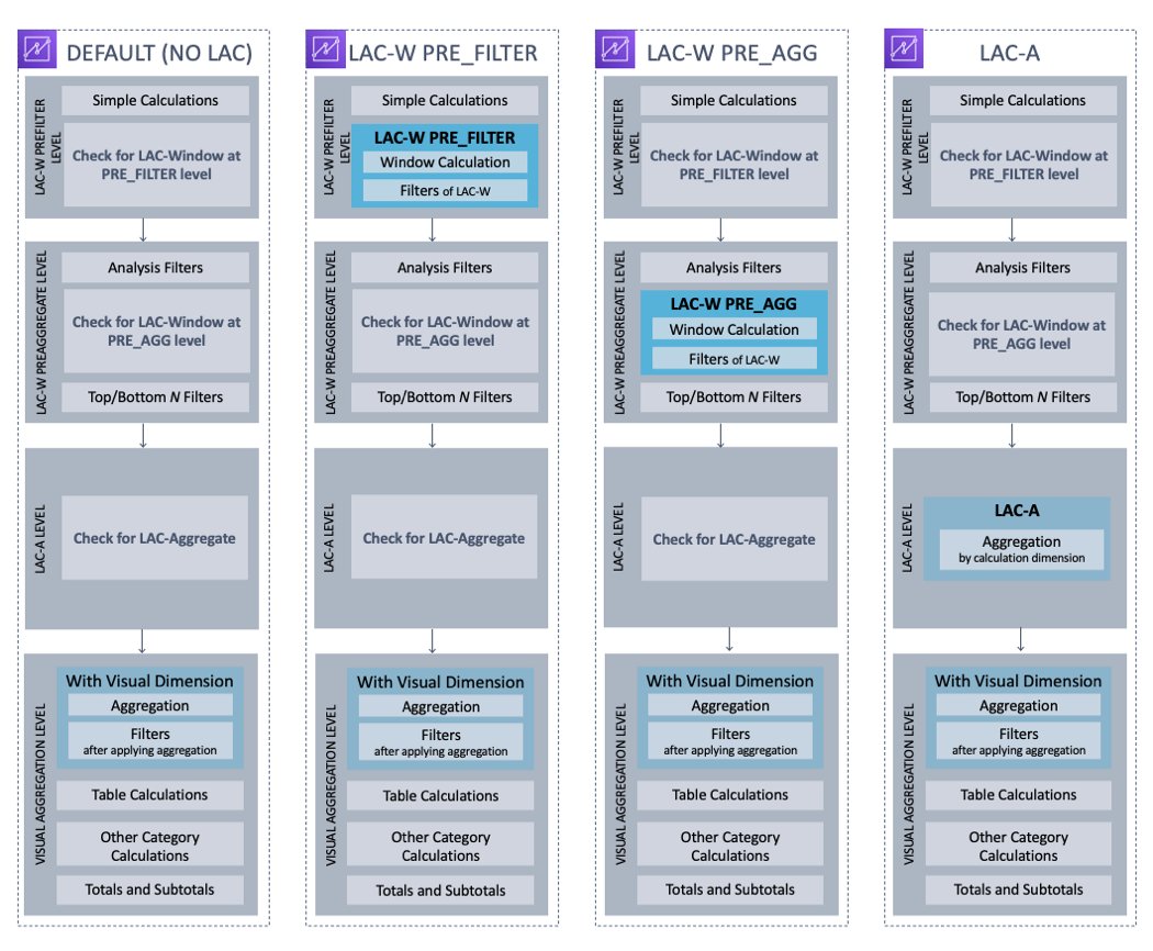
Every time you open or update an analysis, QuickSight evaluates everything that is configured in the analysis in a specific sequence, and translates the configuration into a query that a database engine can run. This is the order of evaluation. The level of complication depends on how many elements are embedded in a visual, multiplied by the number of visuals plus the interactives between the visuals. But if we abstract the concept, the order of evaluation logic can be demonstrated by the following chart.

In the first DEFAULT route, QuickSight evaluates simple calculations at row level for the raw dataset, then it applies the WHERE filters. After that, based on what dimensions are added to the visual, QuickSight evaluates the aggregation for the selected measures at visual dimensions and applies HAVING filters. Table calculations such as running total or percent of total then get evaluated after the visual is formed, with the subtotal and total calculated last.

Sometimes, you may want the analytical steps to be conducted with a different sequence. For example, you may want to do an aggregation before the data being filtered, or do an aggregation first for some specific dimensions and then aggregate again for the visual dimensions. Based on those different needs, QuickSight offers three variations of order of evaluation (as shown in the preceding chart). Specifically, you can use the key words of PRE_FILTER to add a calculation step before the WHERE filter, use PRE_AGG to add a calculation step before the visual aggregation, or use a whole suite of level-aware calculation-aggregation functions to define an aggregation at independent dimensions, and then aggregate them at the visual dimension (a nested aggregation).

Most of the time, your visuals will include more than one calculated field. You’ll want to be careful to define each of them and understand how they’re interacting with the visuals and with different filters. Applying a filter before or after a window function can generate totally different results and business meanings.

With all the background introduced, now let’s talk about the new LAC functions and their capabilities, and demonstrate several typical use cases.

Level-aware calculations (LAC)

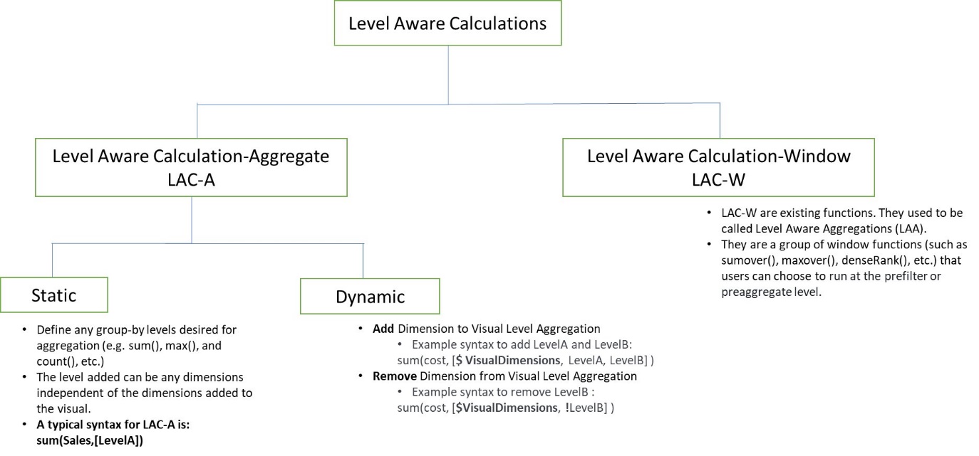
There are two groups of LAC functions:

  • Level-aware calculations-aggregate functions (LAC-A) – These are our newly launched functions. By adding one argument into an existing aggregate function (for example, sum(), max(), or count()), you can define any group-by dimensions you desire for the aggregation. A typical syntax for LAC-A is sum(measure,[group_field_A]). With LAC-A, you can add an aggregation step before the visual aggregation. The added layer can be fixed, which is independent of the visual dimension. It also can be dynamically interacting with the visual dimensions. We give some detailed examples later in this post. For a list of supported aggregation functions, refer to Level-aware calculation – aggregate (LAC-A) functions.
  • Level-aware calculation-window functions (LAC-W) – These are the existing functions. They used to be called level-aware aggregations (LAA). We recently changed its name to better reflect the function nature, due to underlying difference between window functions and aggregate functions. LAC-W is a group of window functions (such as sumover(), maxover(), and denseRank()) where using a third parameter, you can choose to run the calculation at the PRE_FILTER or PRE-AGG stage. A typical syntax for LAC-W is sumOver(measure,[partition_field_A],pre_agg). For a list of supported window functions, refer to Level-aware calculation – window (LAC-W) functions.

The following high-level diagram shows different branches of LAC. In this post, we mostly focus on the new LAC-A functions.

With the new LAC-A functions, you can run two layers of aggregation calculations. This offers the following benefits:

  • Run aggregation calculations that are independent of the group-by fields in the visual calculation
  • Run aggregation calculations for the dimensions that are NOT in the visual
  • Remove duplication of raw data before running calculations
  • Run aggregation calculations with nested group-by fields dynamically adapting to visual group-by fields

Let’s explore how we can achieve those benefits by demonstrating a few use cases.

Use case #1: Identify orders where actual ordered quantity for a product is higher than the average quantity

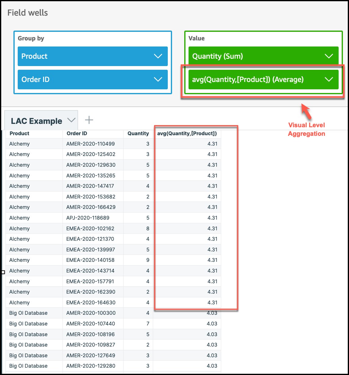
In this case, our visual is at the order level; however, we want to compute the average quantity of a product and use that to display the difference at each individual row/order level. With the LAC-A function, we can easily create an aggregation that is independent of the level in the visual.

We first compute the average quantity sold at product level using the expression of avg(Quantity,[Product]). To do so, change the visual-level aggregation to Average. In this case, visual-level aggregation doesn’t matter because we have product as a column and the LAC-A are at the same level. In the result table, the average quantity value for product is repeated across all orders because this is computed at the product level.

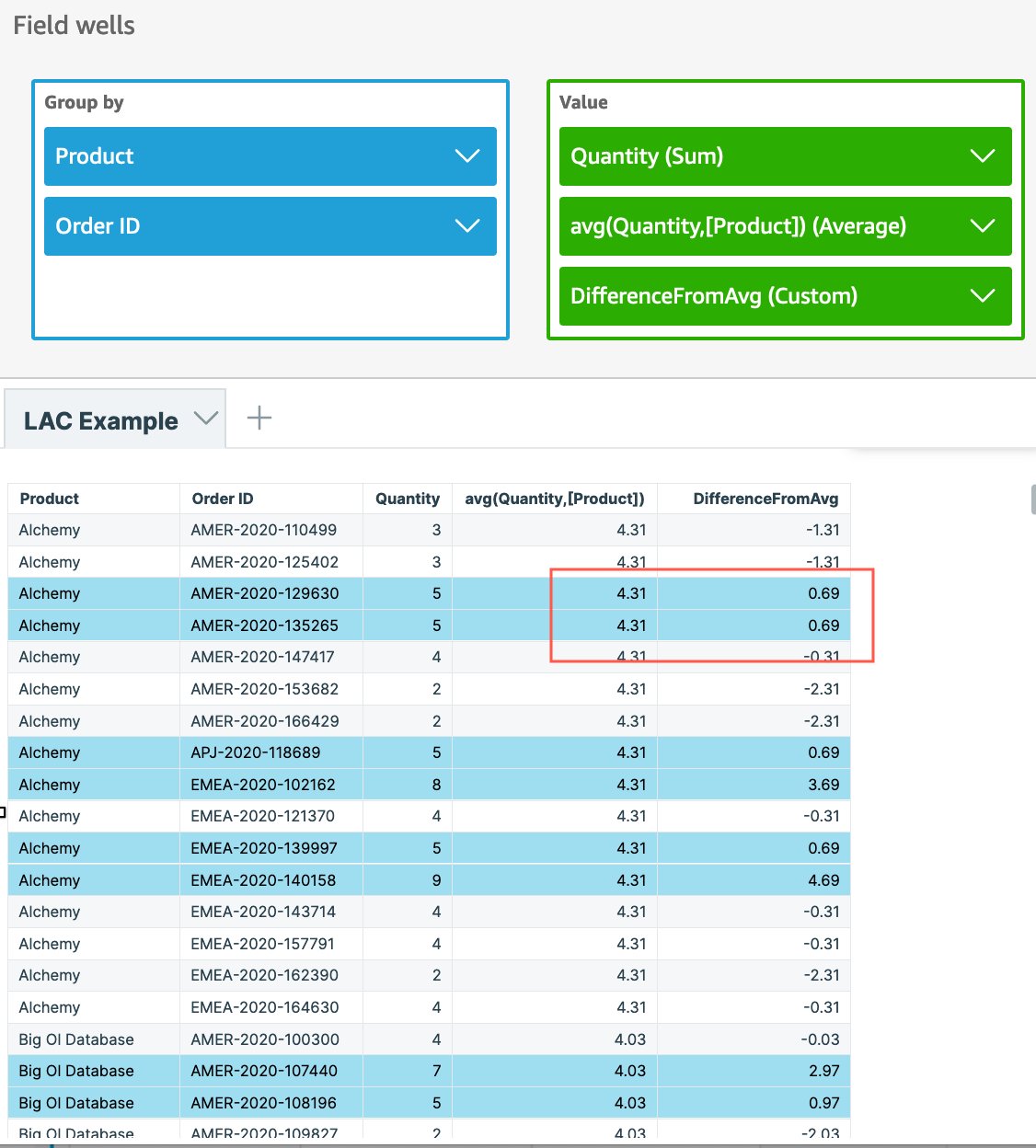
Now that we have computed the average quantity at the product level, we can extend this to compute the difference between actual quantity ordered and the average quantity of product using the expression sum(Quantity) - avg(avg(Quantity,[Product])). This computed difference can then be used to conditionally format the view to highlight orders that have quantity higher than the average quantity of a product.

As seen in this example, although the visual was at the order level, we easily created an aggregation like average quantity of product, which is independent of the level in the visual, and used that to display the difference at each individual row/order level.

Use case #2: Identify the average of total country sales by region

Here we want to aggregate the sales for each country and then compute the average of country-level sales at region level using the same dataset.

With the LAC-A function, we can easily create an aggregation at a dimension level that is NOT in the visual. In this example, although country is not included in the visual, the LAC-A function first aggregates the sales at the country level and then the visual-level calculation generates the average number for each region. Within QuickSight, we can implement this in two ways.

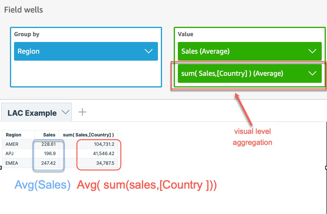
Option 1: Nest the LAC-A with visual-level aggregate functions

Create a calculated column to compute sales at country level by using the expression of sum(Sales,[Country] ), then add the calculation to the visual and change the aggregation to Average, as shown in the following screenshot. Note that if we don’t use LAC-A to specify the level, the average sales are calculated at the lowest granular level (the base level of the dataset) for each region. That’s why the numbers are significantly smaller for the sales column.

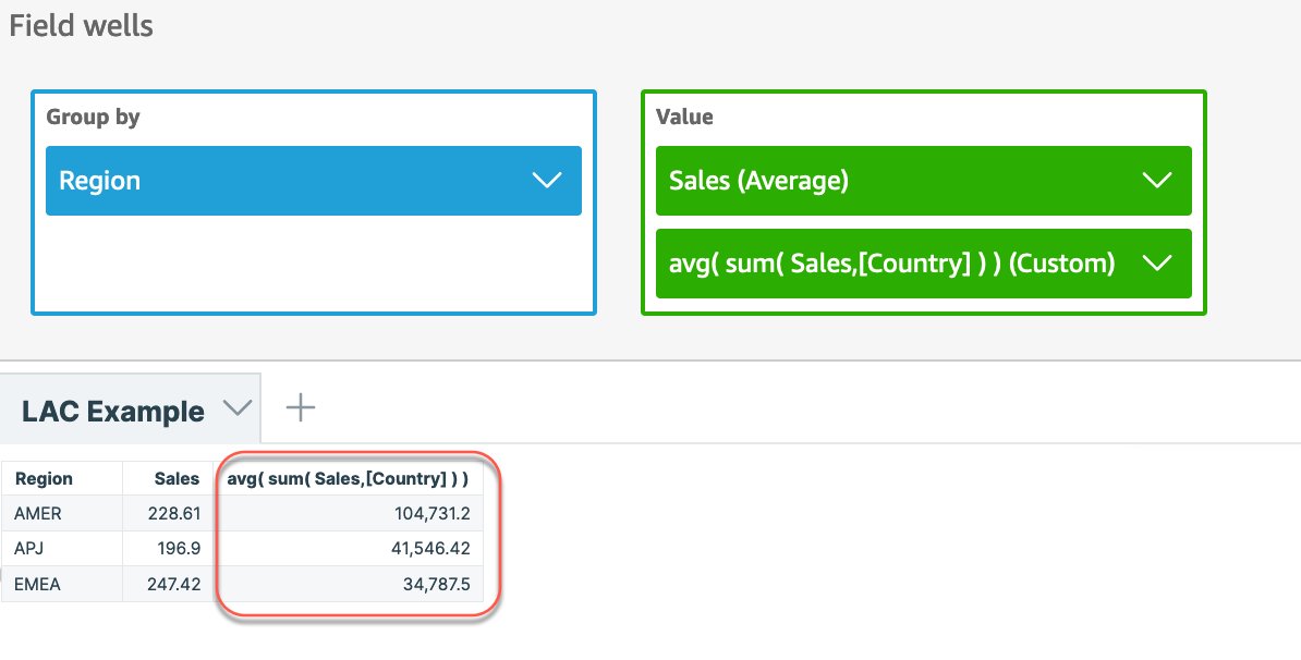
Option 2: Use LAC-A combined with other aggregate functions and nest them in the calculated column

Create a calculated column to compute sales at country level by using the expression sum(Sales,[Country]) and then nest that with additional aggregation, in this case Average, by using the expression avg(sum(Sales,[Country])).

Use case #3: Calculate total and average for a denormalized dataset with duplications

LAC-A calculations are designed to effectively handle duplicates in data while performing computation. It allows you to perform computations like average without the need for explicit handling of duplicates in data.

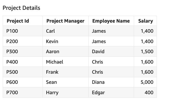
Consider a dataset that has employee and project details along with each employee’s salary. An employee can be associated with multiple projects, as shown in the following example.

Now let’s calculate total employee salary, average employee salary, and minimum and maximum salary using this sample dataset.

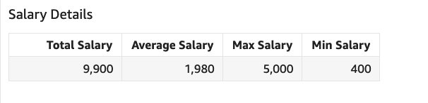
To compute total and average, we have to consider each employee’s salary just once even though an employee can be part of multiple projects and the salary for the employee can get duplicated across these projects. We can easily achieve this using LAC-A to compute the maximum of the salary at the employee level and then use that to compute the total and average.

Create a calculated column called Total Salary using the expression sum(max(Salary,[{Employee Name}])) and create another calculated column called Average Salary using avg(max(Salary,[{Employee Name}])). We can easily calculate Min Salary using the expression min(Salary) and Max Salary using max(Salary).

If we try to solve this without using LAC-A, we have to explicitly handle salary duplication in our calculation, and we have to go through multiple steps to get to the final result. Refer to the QuickSight Community blog for a similar use case.

Dynamic group keys for LAC-A

In addition to defining a static level of aggregation as seen in the preceding examples, you can also dynamically add or remove dimensions from the visual level group-by fields. The following are example syntax for a dynamic level:

  • Add dimensions to the visual dimensions with sum(cost, [$VisualDimensions, LevelA, LevelB])
  • Remove dimensions from the visual dimensions with sum(cost, [$VisualDimensions, !LevelC, !LevelD])

This capability brings a lot of flexibility and scalability for you to make the LAC even more powerful. Firstly, you can define one LAC calculated field and reuse it across multiple visuals with similar business intents. Additionally, if you’re building the visuals and keep adding or deleting the visual fields, you don’t need to edit the LAC-A calculated field each time, and the LAC-A will automatically adjust to the visual dimensions and give the right output.

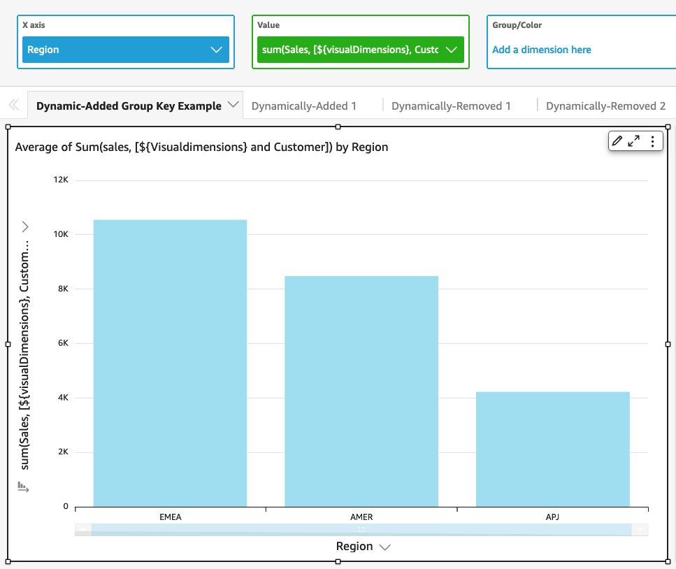
Use case #4: Identify average sales of customers within each region or country

To compute this, we can use the dynamic expression Sum(Sales, [$VisualDimensions, Customers]). This is because each customer has purchases in more than one region. We need to calculate the customer average sales only within each region. We can reuse the same expression in a different visual with country as the visual dimension if we want to calculate average sales of customers within each country.

Use Average as the visual-level metric with Group by as Region to get the region-level average. In this case, “$visualDimensions” is adapted to Region. So the expression is equivalent to Sum(Sales, [Region, Customers]) in this visual.

If you have a similar visual with the Country dimension, then the dynamic expression is equivalent to Sum(Sales, [Country, Customers]). Reusing the same expression in different visuals saves us a lot of time, especially when we want to build similar visuals with slightly different business context.

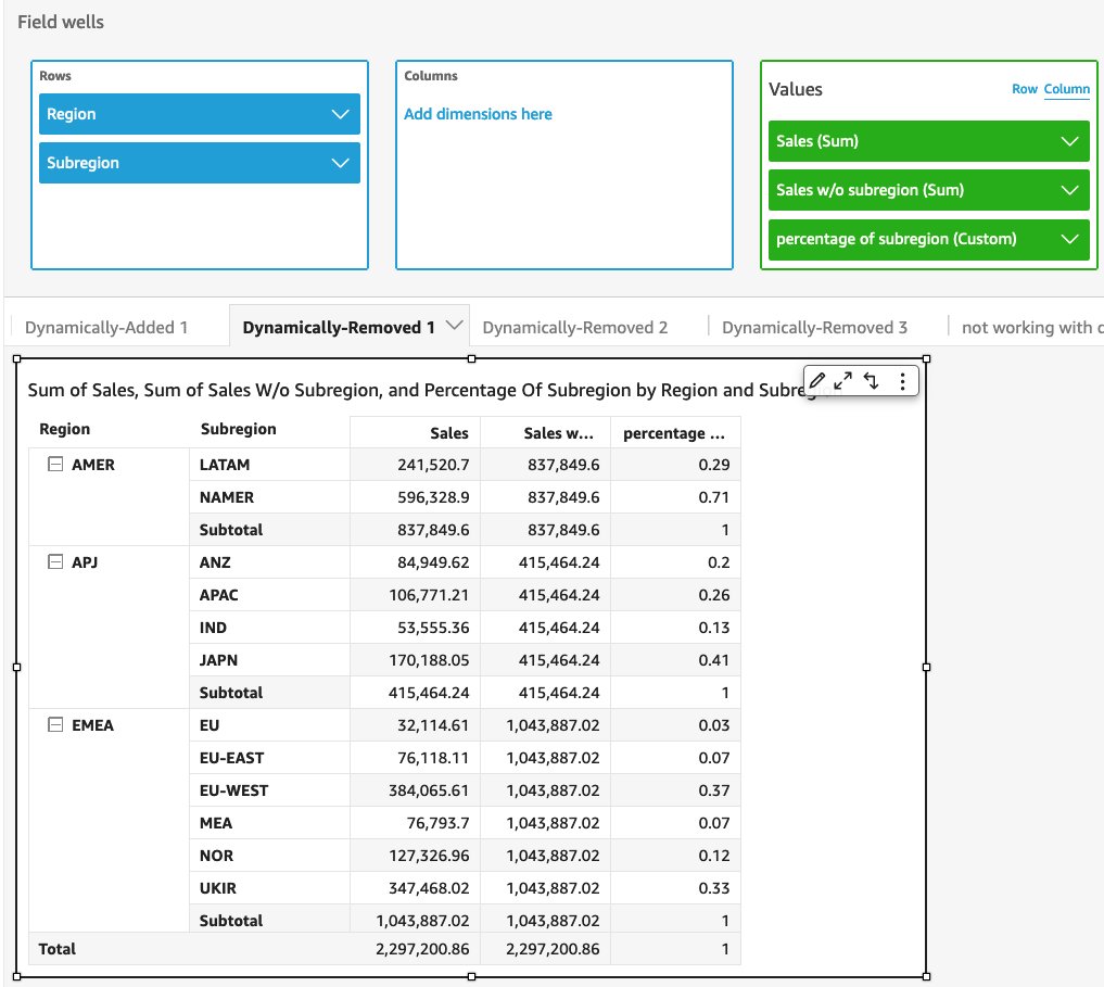
Use case #5: Identify the sales percentage of each subregion compared to region level

In this example, we want to calculate the percentage of sales for each subregion, comparing with the total region sales. You can use the fixed dimension as we mentioned before, but imagine a situation when you want to include more dimensions into the visual such as product, year, or supplier. Using the dynamic group key by removing only {subregion} from the visual dimensions makes the exploration process much easier and quicker.

First, create an expression to calculate the sum of sales without the subregion level using sum(Sales, [$visualDimensions, !subregion]), then calculate the percentage using sum(Sales) / sum(sum(Sales, [$visualDimensions, !subregion])).

Conclusion

In this post, we introduced new QuickSight LAC-A functions, which enable powerful and advanced aggregations with user-defined dimensions. We introduced the QuickSight order of evaluation, and walked through three use cases for LAC-A static keys and two use cases of LAC-A dynamic keys. Level-aware calculations are now generally available in all supported QuickSight Regions.

We look forward to your feedback and stories on how you apply these calculations for your business needs.


About the Authors

Karthik Tharmarajan is a Senior Specialist Solutions Architect for Amazon QuickSight. Karthik has over 15 years of experience implementing enterprise business intelligence (BI) solutions and specializes in integration of BI solutions with business applications and enable data-driven decisions.

Emily Zhu is a Senior Product Manager-Tech at Amazon QuickSight, AWS’s cloud-native, fully managed SaaS BI service. She leads the development of the QuickSight analytics and query experience. Before joining AWS, she worked in the Amazon Prime Air drone delivery program and the Boeing company as senior strategist for several years. Emily is passionate about the potential of cloud-based BI solutions and looks forward to helping customers advance in their data-driven strategy making.

Feng Han is a Software Development Manager in AWS QuickSight Query Platform team. He focuses on query generation platform and advanced function calculation, and is leading the team to next generation of calculation engine.

BloomIP Automatically Identifies production issues with Amazon DevOps Guru

Post Syndicated from David Ernst original https://aws.amazon.com/blogs/devops/bloomip-automatically-identifies-production-issues-with-amazon-devops-guru/

Operational excellence is critical for BloomIP’s customers. In this post, you will see how we built a solution to automate the detection of trends and issues in production workloads by implementing Amazon DevOps Guru for our clients.

BloomIP ensures your business is ready for what’s ahead, with security, scalability, performance, and cost control. We are cloud solutions partner that gets to know both the people and processes in your business.

The Challenge

Identifying operational issues within applications and services is time-consuming. This requires developers and cloud engineers to spend valuable time manually debugging using multiple tools. We needed to quickly identify any operational issues related to our clients applications, including any load balancer errors or user delays in accessing their application. Ensuring the application is up and running during certain times of the day is crucial to the success of our client’s business. We needed to identify any downtime or performance patterns and quickly address any related issues.

Analyzing an AWS environment after any incident requires a combination of tools such as Amazon CloudWatch, AWS Config, AWS CloudTrail, AWS CloudFormation, and AWS X-Ray. We spend hours pouring over the information in each tool to try to identify patterns and troubleshooting steps. Still, identifying issues that correlate between those tools is a manual process.

Automating Identification of Operational Issues

To address the challenges of tedious and manual processes of analyzing different tools to identify patterns, we implemented Amazon DevOps Guru  for many of our clients. Amazon DevOps Guru helps us automatically ingests all related data from the services mentioned above and applies Machine Learning techniques to analyze and recommend fixes for abnormal behaviors. Amazon DevOps Guru organizes its findings into reactive and proactive insights.

We capture Amazon DevOps Guru Insights as events using Amazon EventBridg, and send them to an  Amazon SNS Topic, which then notifies us via email and Slack.

Architecture diagram showing a typical 3 tier web app using AWS services and integrating the application with Amazon DevOps Guru, Amazon Eventbridge and Amazon SNS Topic to send send notifications via Email and Slack

Figure 1. Architecture diagram

Results

BloomIP is leveraging DevOps Guru to scale its operations across multiple customers. Amazon DevOps Guru was easy to enable; it provides us with a single console experience to search and visualize operational data. In addition to detecting anomalies, we can see graphs and timelines related to the numerous anomalous metrics and more contextual information such as relevant events and log snippets. This helps us quickly understand the anomaly scope. Because it integrates data across multiple sources such as Amazon CloudWatch, AWS Config, AWS CloudTrail, AWS CloudFormation, and AWS X-Ray, Amazon DevOps Guru reduces the need for us to use numerous tools.

“We were looking at a way to effortlessly scale our observability needs across multiple clients while ensuring we had the proper coverage. DevOps Guru gives us additional insight and assurance by quickly pointing out anomalies in our client’s environments. With ML-powered recommendations, DevOps Guru has allowed us to remediate repeated production issues automatically. ” – Joshua Haynes, Director of Engineering, BloomIP

Conclusion

Amazon DevOps Guru provides BloomIP with a streamlined approach to visualize operational data by integrating data across multiple sources supporting Amazon CloudWatch, AWS Config, AWS CloudTrail, AWS CloudFormation, and AWS X-Ray and reduces the need to use multiple tools. DevOps Guru gives you a single-console dashboard to look for and visualize anomalies in your operational data.

Start monitoring your AWS applications with AWS DevOps Guru today using this link

About the authors:

David Ernst

David is a Sr. Specialist Solution Architect – DevOps, with 20+ years of experience in designing and implementing software solutions for various industries. David is an automation enthusiast and works with AWS customers to design, deploy, and manage their AWS workloads/architectures.

Abdullahi Olaoye

Abdullahi is a Senior Cloud Architect at AWS Professional Services where he works with customers of different scales to design and build IT solutions that solve business challenges. When he’s not working, he enjoys spending time with his family, traveling and learning history of different varieties through documentaries and podcasts.

Reducing Risk In The Cloud with Agentless Vulnerability Management

Post Syndicated from Alon Berger original https://blog.rapid7.com/2022/11/28/reducing-risk-with-agentless-cloud-vulnerability-management/

Reducing Risk In The Cloud with Agentless Vulnerability Management

In order to gain visibility into vulnerabilities in their public cloud environments, many organizations still rely on agent or network-based scanning technology that was initially built for traditional infrastructure and endpoints.

These methods often struggle to keep up with the speed of change and scale of complex, and constantly changing cloud environments, forcing infrastructure teams to constantly play catch up and avoid significant blindspots caused by unprotected workloads.

Vulnerability management in the cloud starts with continuous discovery of the container images and host workloads that may contain them and the supporting resources that control how they are launched.  The assessment step produces  long lists of vulnerabilities that can lack the necessary context to help prioritize and accurately route the issue to the correct owners for remediation.

Getting Better Visibility and Control

Rapid7’s InsightCloudSec now addresses all these challenges and provides agentless vulnerability assessment capabilities for cloud-based container workloads and hosts.  Building on InsightCloudSec’s industry leading cloud resource discovery technology, we’ve unleashed the latest generation agentless methods for assessing vulnerabilities on Containers using side-scanning and on Hosts using image snapshotting.  Combined, this fully enables security teams to quickly identify where the vulnerabilities exist across their cloud infrastructure, what resources are responsible for managing the dynamic workloads that launch them, and the tools to manage response prioritization and remediation.

InsightCloudSec’s vulnerability management  capabilities are  purpose-built for cloud-native environments and leverage Rapid7’s proven vulnerability management expertise and intelligence.  Our agentless approach  reduces the unnecessary overhead of agent management on highly ephemeral cloud resources.

Vulnerability Management with Rapid7’s InsightCloudSec

Vulnerability management with InsightCloudSec focuses on container and host-based workloads found in production environments, where the risk of exploitation is the highest. The solution leverages event-driven detection capabilities, allowing teams to maintain an up-to-the-minute inventory of all resources in production. This in turn minimizes blind spots and allows for more trustworthy reporting.

The solution automatically analyzes new container images and host instances upon deployment and provides detailed intelligence and remediation guidance for known vulnerabilities. InsightCloudSec then periodically revalidates running hosts against the newest vulnerability data to detect and protect against drift.

Our comprehensive vulnerability detection spans operating systems, installed software packages, network services, and open-source software libraries and packages typically used as dependencies in these environments, providing customers with the broadest coverage available in the market.

Agentless Container and Host Workload Assessment

With agentless Vulnerability assessment, security teams gain robust, continuous visibility into what vulnerabilities exist in their cloud environment, without having to include an agent in their container and host golden images. We discover new container images and host instances in near-real-time and immediately gather the information necessary to perform the assessment without waiting for a scheduled scan window or impacting the performance of the live workloads.  

When new container images are detected in the monitored registries, InsightCloudSec performs a side-scan on them to index the inventory of operating system and installed software packages as well as any other dependent libraries that exist on which we can detect vulnerabilities.

In the same way, once a new running host (VM) instance is detected, InsightCloudSec fetches the workload’s runtime storage layer using remote harvesting and automated snapshot triggering to gather the data required for vulnerability assessment.

By combining workloads metadata gathered from cloud provider APIs with container and host vulnerability data, we are able to provide contextualized vulnerability reports and deep visibility of where they exist in cloud environments, allowing security teams to respond to those impacting the most critical applications and cloud accounts.

Conclusion

Rapid7 and InsightCloudSec strive to help security and operation teams apply proper processes and procedures across the deployment pipeline, allowing them to quickly respond to vulnerabilities of any sort and severity.

With an accurate assessment of detected vulnerabilities and intelligent, automated routing for faster remediation, our solution empowers teams to have a robust and continuous visibility into vulnerabilities that exist in their cloud environments.

Want to learn more? Click here.

Scale AWS SDK for pandas workloads with AWS Glue for Ray

Post Syndicated from Abdel Jaidi original https://aws.amazon.com/blogs/big-data/scale-aws-sdk-for-pandas-workloads-with-aws-glue-for-ray/

AWS SDK for pandas is an open-source library that extends the popular Python pandas library, enabling you to connect to AWS data and analytics services using pandas data frames. We’ve seen customers use the library in combination with pandas for both data engineering and AI workloads. Although pandas data frames are simple to use, they have a limitation on the size of data that can be processed. Because pandas is single-threaded, jobs are bounded by the available resources. If the data you need to process is small, this won’t be a problem, and pandas makes analysis and manipulation simple, as well as interactions with many other tools that support machine learning (ML) and visualization. However, as your data size scales, you may run into problems. This can be especially frustrating if you’ve created a promising prototype that can’t be moved to production. In our work with customers, we’ve seen many projects, both in data science and data engineering, that are stuck while they wait for someone to rewrite using a big data framework such as Apache Spark.

We are excited to announce that AWS SDK for pandas now supports Ray and Modin, enabling you to scale your pandas workflows from a single machine to a multi-node environment, with no code changes. The simplest way to do this is to use AWS Glue with Ray, the new serverless option to run distributed Python code announced at AWS re:Invent 2022. AWS SDK for pandas also supports self-managed Ray on Amazon Elastic Compute Cloud (Amazon EC2).

In this post, we show you how you can use pandas to connect to AWS data and analytics services and manipulate data at scale by running on an AWS Glue with Ray job.

Overview of solution

Ray is a unified framework that enables you to scale AI and Python applications. The goal of the project is to take any Python code that’s written on a laptop and scale the workload on a cluster. This innovative framework opens the door to big data processing to a new audience. Previously, the only way to process large datasets on a cluster was to use tools such as Apache Hadoop, Apache Spark, or Apache Flink. These frameworks require additional skills because they provide their own programming model and often require languages such as Scala or Java to fully take advantage of the advanced capabilities. With Ray, you can just use Python to parallelize your code with few modifications.

Although Ray opens the door to big data processing, it’s not enough on its own to distribute pandas-specific methods. That task falls to Modin, a drop-in replacement of pandas, optimized to run in a distributed environment, such as Ray. Modin has the same API as pandas, so you can keep your code the same, but it parallelizes workloads to improve performance.

With today’s announcement, AWS SDK for pandas customers can use both Ray and Modin for their workloads. You have the option of loading data into Modin data frames, instead of regular pandas data frames. By configuring the library to use Ray and Modin, your existing data processing scripts can distribute operations end-to-end, with no code changes. AWS SDK for pandas takes care of parallelizing the read and write operations for your files across the compute cluster.

To use this feature, you can install the release candidate version of awswrangler with the ray and modin extras:

pip install "awswrangler[modin,ray]==3.0.0rc2"

Once installed, you can use the library in your code by importing it with the following statement:

import awswrangler as wr

When you run this code, the SDK for pandas looks for an environmental variable called WR_ADDRESS. If it finds it, it uses this value to send the commands to a remote cluster. If it doesn’t find it, it starts a local Ray runtime on your machine.

The following diagram shows what is happening when you run code that uses AWS SDK for pandas to read data from Amazon Simple Storage Service (Amazon S3) into a Modin data frame, perform a filtering operation, and write the data back to Amazon S3, using a multi-node cluster.

In the first phase, each node reads one or more input files and stores them in memory as blocks. During this phase, the head node builds a mapping reference that tracks the location of each block on the worker nodes. In the second phase, a filter operation is submitted to each node, creating a subset of the data. Finally, each worker node writes its blocks to Amazon S3.

It’s important to note that certain data frame operations (for example groupby or join) may result in the data being shuffled across nodes. Shuffling will also happen if you do partitioned or bucketed writes. This tends to slow down the job because data needs to move between nodes.

If you want to create your own Ray cluster on Amazon EC2, refer to the tutorial Distributing Calls on Ray Remote Cluster. The rest of this post shows you how to run AWS SDK for pandas and Modin on an AWS Glue with Ray job.

Use AWS Glue with Ray

Because AWS Glue with Ray is a fully managed environment, it’s a simple way to run jobs. Both AWS SDK for pandas and Modin are pre-loaded, you don’t need to worry about cluster management or installing the right set of dependencies, and the job auto scales with your workload. To get started, complete the following steps:

  1. Choose Launch Stack to provision an AWS CloudFormation stack in your AWS account:
    launch cloudformation stack
    Note that while in preview, AWS Glue with Ray is available in a limited set of AWS Regions.The stack takes about 3 minutes to complete. You can verify that everything was successfully deployed by checking that the CloudFormation stack shows the status CREATE_COMPLETE.
  2. Navigate to AWS Glue Studio to find an AWS Glue job named GlueRayJob with the following script.
  3. Choose Run to start the job and navigate to the Runs tab to monitor progress.

Here, we break down the script and show you what happens at each stage when we run this code on AWS Glue with Ray. First, we import the library:

import awswrangler as wr

At import, AWS SDK for pandas detects if the runtime supports Ray, and automatically initializes a Ray cluster with the default parameters. In this case, because we’re running on AWS Glue with Ray, AWS SDK for pandas automatically uses the Ray cluster with no extra configuration needed. Advanced users can override this process, however, by starting the Ray runtime before the import command.

Next, we read Amazon product data in Parquet format from Amazon S3 and load it into a distributed Modin data frame:

# Read Parquet data (1.2 Gb Parquet compressed)
df = wr.s3.read_parquet(
    path=f"s3://amazon-reviews-pds/parquet/product_category={category.title()}/",
)

Simple data transformations on the data frame are applied next. Modin data frames implement the same interface as pandas data frames, allowing you to perform familiar pandas operations at scale. First, we drop the customer_id column, then we filter for a subset of the reviews that received five-star ratings:

# Drop the customer_id column
df.drop("customer_id", axis=1, inplace=True)

# Filter reviews with 5-star rating
df5 = df[df["star_rating"] == 5]

The data is written back to Amazon S3 in Parquet format, partitioned by year and marketplace. The dataset=True argument ensures that an associated Hive table is also created in the AWS Glue metadata catalog:

# Write partitioned five-star reviews to S3 in Parquet format
wr.s3.to_parquet(
    df5,
    path=f"s3://{bucket_name}/{category}/",
    partition_cols=["year", "marketplace"],
    dataset=True, 
    database=glue_database,
    table=glue_table, 
)

Finally, a query is run in Amazon Athena, and the S3 objects resulting from this operation are read in parallel into a Modin data frame:

# Read the data back to a Modin df via Athena
df5_athena = wr.athena.read_sql_query(
    f"SELECT * FROM {glue_table}",
    database=glue_database,
    ctas_approach=False, 
    unload_approach=True, 
    workgroup=workgroup_name,
    s3_output=f"s3://{bucket_name}/unload/{category}/",
)

The Amazon CloudWatch logs of the job provide insights into the performance achieved from reading blocks in parallel in a multi-node Ray cluster.

For simplicity, this example showcased Amazon S3 and Athena APIs only, but AWS SDK for pandas supports other services, including Amazon Timestream and Amazon Redshift. For a full list of the APIs that support distribution, refer to Supported APIs.

Clean up AWS resources

To prevent unwanted charges to your AWS account, you can delete the AWS resources that you used for this example:

  1. On the Amazon S3 console, empty data from both buckets with prefix glue-ray-.
  2. On the AWS CloudFormation console, delete the SDKPandasOnGlueRay stack.

The resources created as part of the stack are automatically deleted with it.

Conclusion

In this post, we demonstrated how you can run your workloads at scale using AWS SDK for pandas. When used in combination with AWS Glue with Ray, this gives you access to a fully managed environment to distribute your Python scripts. We hope this solution can help with migrating your existing pandas jobs to achieve higher performance and speedups across multiple data stores on AWS.

For more examples, check out the tutorials in the AWS SDK for pandas documentation.


About the Authors

Abdel Jaidi is a Senior Cloud Engineer for AWS Professional Services. He works on open-source projects focused on AWS Data & Analytics services. In his spare time, he enjoys playing tennis and hiking.

Anton Kukushkin is a Data Engineer for AWS Professional Services based in London, United Kingdom. He works with AWS customers, helping them build and scale their data and analytics.

Leon Luttenberger is a Data Engineer for AWS Professional Services based in Austin, Texas. He works on AWS open-source solutions that help our customers analyze their data at scale.

Lucas Hanson is Senior Cloud Engineer for AWS Professional Services. He focuses on helping customers with infrastructure management and DevOps processes for data management solutions. Outside of work, he enjoys music production and practicing yoga.

New – Failover Controls for Amazon S3 Multi-Region Access Points

Post Syndicated from Jeff Barr original https://aws.amazon.com/blogs/aws/new-failover-controls-for-amazon-s3-multi-region-access-points/

We launched Amazon S3 Multi-Region Access Points to give you a global endpoint that spans S3 buckets in multiple AWS Regions. With S3 Multi-Region Access Points, you can build multi-region applications with the same simple architecture used in a single Region. This cool and powerful feature uses AWS Global Accelerator to monitor network congestion and connectivity, and to route traffic to the closest copy of your data. In the event that connectivity between a client and a bucket in a particular Region is lost, the Multi-Region Access Point will automatically route all traffic to the closest bucket (synchronized via S3 Replication) in another Region.

In addition to the use case that I just described, customers have told us that they want to build highly available multi-region apps and need explicit control over failover and failback.

New Failover Controls
Today we are adding failover controls for Multi-Region Access Points. These controls let you shift S3 data access request traffic routed through an Amazon S3 Multi-Region Access Point to an alternate AWS Region within minutes to test and build highly available applications for business continuity.

The existing Multi-Region Access Point model treats all of the Regions as active and can send traffic to any of them. The model that we are introducing today lets you designate Regions as either active or passive. Buckets in active Regions receive traffic (GET, PUT, and other requests) from the Multi-Region Access Point, buckets in passive Regions don’t. Amazon S3 Cross-Region Replication operates regardless of the active or passive status of a Region with respect to a particular Multi-Region Access Point.

To get started, I create a new Multi-Region Access Point that refers to two or more S3 buckets in distinct AWS Regions. I enter a name for my Multi-Region Access Point (jbarr-mrap-1), and choose the buckets:

I leave the Amazon S3 Block Public Access settings as-is, and click Create Multi-Region Access Point:

Then I wait until my Multi-Region Access Point is ready (generally just a few minutes):

By default, my new Multi-Region Access Point routes traffic to all of the buckets, and behaves as it did before we launched this new feature. However, I can now exercise control over routing and failover. I click on the Multi-Region Access Point, and on the Replication and failover tab (which used to be just a Replication tab). The map now allows me to see my replication rules and my failover status:

I can scroll down to view, create, and modify my replication rules:

As you can see, the replication rules that I created for this demo preserve the storage class. S3 Intelligent-Tiering is generally a better choice, since I would get automatic cost savings without increased data retrieval costs after a failover. I can use S3 Replication metrics to make sure that my replication rules are proceeding as expected. Also, S3 Replication Time Control provides a predictable replication time (backed by an SLA), and should also be considered.

The tab also includes the failover configuration:

To change my failover configuration, I select the buckets of interest and click Edit failover configuration. My application runs in the Asia Pacific (Tokyo) Region and makes use of a bucket there, so I leave the Tokyo Region active and make the others passive:

All is well until one fine day Godzilla wakes up and eats all of the submarine cables in and around Tokyo. I quickly pull up the console, return to the Failover configuration, select the active Tokyo Region and the passive Osaka Region, and click Failover:

I confirm my intent, click Failover again, and the failover is complete within two minutes:

Later, after Godzilla has been subdued and the cables have been repaired, I can fail back to the original bucket in the Tokyo Region:

Things to Know
Here are a couple of things to keep in mind as you start to make use of this important new AWS feature:

Active/Passive – There must be at least one active Region at all times.

CLI & API Access – You can initiate a failover programmatically by calling SubmitMultiRegionAccessPointRoutes. You can retrieve the current set of routes by calling GetMultiRegionAccessPointRoutes. The endpoints for these APIs are available in the US East (N. Virginia), US West (Oregon), Asia Pacific (Sydney, Tokyo), and Europe (Ireland) Regions.

Pricing – There is no extra charge for this feature beyond the use of the new APIs, which are billed as standard S3 GET and PUT requests. For S3 Multi-Region Access Point usage prices, see the Pricing tab of the Amazon S3 Pricing page.

Regions – This feature is available in all AWS Regions where Multi-Region Access Points are currently available.

Jeff;

Automated Data Discovery for Amazon Macie

Post Syndicated from Sébastien Stormacq original https://aws.amazon.com/blogs/aws/automated-data-discovery-for-amazon-macie/

Today, we announce automated data discovery for Amazon Macie. This new capability allows you to gain visibility into where your sensitive data resides on Amazon Simple Storage Service (Amazon S3) at a fraction of the cost of running a full data inspection across all your S3 buckets.

At AWS, security is our first priority. The security of the infrastructure itself, but also the security of your data. We give you access to services to manage identities and access, to protect the network and your applications, to detect suspicious activities, to protect your data, and to report on and monitor your compliance status.

Amazon Macie is a data security service that discovers sensitive data using machine learning and pattern matching and enables visibility and automated protection against data security risks. You use Amazon Macie to protect your data in S3 by scanning for the presence of sensitive data, such as names, addresses, and credit card numbers, and continually monitoring for properly configured preventative controls, such as encryption and access policies. Amazon Macie generates alerts when it detects publicly accessible buckets, unencrypted buckets, or buckets shared with an AWS account outside of your organization. You may also configure Amazon Macie to scan your S3 to run full sensitive data discovery scans on your S3 buckets to provide visibility into where sensitive data resides.

But customers operating at scale told us it is difficult to know where to start. When employees and applications add new buckets and generate petabytes of data on a daily basis, what should be scanned first?

Automated data discovery automates the continual discovery of sensitive data and potential data security risks across your entire set of buckets aggregated at AWS Organizations level.

When you enable automated discovery in the console, Macie starts to evaluate the level of sensitivity of each of your buckets and highlights any data security risks. Automated data discovery introduces intelligent and fully managed data sampling to provide an optimized sample rate that meaningfully reduces the amount of data that needs to be analyzed. This reduces the cost of discovering S3 buckets containing sensitive data compared to the cost of full data inspection.

You can tune automated data discovery to only identify the types of sensitive data that are relevant for your use case by choosing from over 100 managed sensitive data types, such as personally identifiable information (PII) and financial records with specific formats for multiple countries. For example, you can enable detection of Spanish or Swedish driving license numbers and choose to ignore US Social Security numbers, depending on your use cases. When the specific type of data you manage is not on our list, you can create custom data types that may be unique to your business, such as employee or patient identification numbers.

Let’s See It in Action
Automated data discovery is on by default for all new Amazon Macie customers, and existing Macie customers can enable it with one click in the AWS Management Console of the Amazon Macie administrator account. There is a 30-day free trial, and you can always opt out at the administrator level.

I can enable or disable the capability from the Automated discovery entry–under Settings–on the left side navigation menu. The Status section reveals the current status.

Automated data discovery for Amazon Macie - Enable

On the same page, I can configure the list of managed data identifiers. I can turn on or off individual types of data among more than one hundred managed data identifier types. I can also configure new ones. I select Edit on the Managed data identifiers section to include or exclude additional data identifiers.

Automated data discovery for Amazon Macie - include or exclude data identifiers

If I have some buckets with lots of objects and others with a few, Macie won’t spend all its time inspecting one really large bucket at the expense of other smaller ones. Macie also prioritizes buckets that it knows the least about. For example, if it looked at the majority of objects in a small bucket, that bucket will be deprioritized compared to larger buckets where it has seen proportionally fewer objects.

Automated data discovery can provide an interactive data map of sensitive data distribution in S3 buckets within days of the feature being enabled. This data map refreshes daily as it intelligently picks and scans S3 objects in buckets and spreads the scan effort across the entire S3 estate in a given month.

Here is the Summary section of the Amazon Macie page. It looks like my set of buckets is secured. I have no bucket with public access, and 31 of my buckets might contain sensitive data.

Automated data discovery for Amazon Macie - Summary section

When selecting the S3 buckets section of the navigation menu on the left side, I can see a data map of my buckets. The more red the squares are, the more sensitive data are detected in the buckets. The squares in blue represent buckets with no sensitive data detected so far. From there, I can drill down at bucket level to investigate the details.

Automated data discovery for Amazon Macie - Heat map

Pricing and Availability
When you are new to Amazon Macie, automated data discovery is enabled by default. When you already use Amazon Macie in your organization, you can enable automatic data discovery with one click in the Management Console of the Amazon Macie administrator account.

There is a 30-day free trial period when you enable automatic data discovery on your AWS account. After the evaluation period, we charge based on the total quantity of S3 objects in your account as well as the bytes scanned for sensitive content. Charges are prorated per day. You can disable this capability at any time. The pricing page has all the details.

This new capability is now available in all 21 commercial AWS Regions where Macie is available.

Go and enable Amazon Macie automated data discovery today!

— seb

New – AWS Config Rules Now Support Proactive Compliance

Post Syndicated from Danilo Poccia original https://aws.amazon.com/blogs/aws/new-aws-config-rules-now-support-proactive-compliance/

When operating a business, you have to find the right balance between speed and control for your cloud operations. On one side, you want to have the ability to quickly provision the cloud resources you need for your applications. At the same time, depending on your industry, you need to maintain compliance with regulatory, security, and operational best practices.

AWS Config provides rules, which you can run in detective mode to evaluate if the configuration settings of your AWS resources are compliant with your desired configuration settings. Today, we are extending AWS Config rules to support proactive mode so that they can be run at any time before provisioning and save time spent to implement custom pre-deployment validations.

When creating standard resource templates, platform teams can run AWS Config rules in proactive mode so that they can be tested to be compliant before being shared across your organization. When implementing a new service or a new functionality, development teams can run rules in proactive mode as part of their continuous integration and continuous delivery (CI/CD) pipeline to identify noncompliant resources.

You can also use AWS CloudFormation Guard in your deployment pipelines to check for compliance proactively and ensure that a consistent set of policies are applied both before and after resources are provisioned.

Let’s see how this works in practice.

Using Proactive Compliance with AWS Config
In the AWS Config console, I choose Rules in the navigation pane. In the rules table, I see the new Enabled evaluation mode column that specifies whether the rule is proactive or detective. Let’s set up my first rule.

Console screenshot.

I choose Add rule, and then I enter rds-storage in the AWS Managed Rules search box to find the rds-storage-encrypted rule. This rule checks whether storage encryption is enabled for your Amazon Relational Database Service (RDS) DB instances and can be added in proactive or detective evaluation mode. I choose Next.

Console screenshot.

In the Evaluation mode section, I turn on proactive evaluation. Now both the proactive and detective evaluation switches are enabled.

Console screenshot.

I leave all the other settings to their default values and choose Next. In the next step, I review the configuration and add the rule.

Console screenshot.

Now, I can use proactive compliance via the AWS Config API (including the AWS Command Line Interface (CLI) and AWS SDKs) or with CloudFormation Guard. In my CI/CD pipeline, I can use the AWS Config API to check the compliance of a resource before creating it. When deploying using AWS CloudFormation, I can set up a CloudFormation hook to proactively check my configuration before the actual deployment happens.

Let’s do an example using the AWS CLI. First, I call the StartProactiveEvaluationResponse API with in input the resource ID (for reference only), the resource type, and its configuration using the CloudFormation schema. For simplicity, in the database configuration, I only use the StorageEncrypted option and set it to true to pass the evaluation. I use an evaluation timeout of 60 seconds, which is more than enough for this rule.

aws configservice start-resource-evaluation --evaluation-mode PROACTIVE \
    --resource-details '{"ResourceId":"myDB",
                         "ResourceType":"AWS::RDS::DBInstance",
                         "ResourceConfiguration":"{\"StorageEncrypted\":true}",
                         "ResourceConfigurationSchemaType":"CFN_RESOURCE_SCHEMA"}' \
    --evaluation-timeout 60
{
    "ResourceEvaluationId": "be2a915a-540d-4595-ac7b-e105e39b7980-1847cb6320d"
}

I get back in output the ResourceEvaluationId that I use to check the evaluation status using the GetResourceEvaluationSummary API. In the beginning, the evaluation is IN_PROGRESS. It usually takes a few seconds to get a COMPLIANT or NON_COMPLIANT result.

aws configservice get-resource-evaluation-summary \
    --resource-evaluation-id be2a915a-540d-4595-ac7b-e105e39b7980-1847cb6320d
{
    "ResourceEvaluationId": "be2a915a-540d-4595-ac7b-e105e39b7980-1847cb6320d",
    "EvaluationMode": "PROACTIVE",
    "EvaluationStatus": {
        "Status": "SUCCEEDED"
    },
    "EvaluationStartTimestamp": "2022-11-15T19:13:46.029000+00:00",
    "Compliance": "COMPLIANT",
    "ResourceDetails": {
        "ResourceId": "myDB",
        "ResourceType": "AWS::RDS::DBInstance",
        "ResourceConfiguration": "{\"StorageEncrypted\":true}"
    }
}

As expected, the Amazon RDS configuration is compliant to the rds-storage-encrypted rule. If I repeat the previous steps with StorageEncrypted set to false, I get a noncompliant result.

If more than one rule is enabled for a resource type, all applicable rules are run in proactive mode for the resource evaluation. To find out individual rule-level compliance for the resource, I can call the GetComplianceDetailsByResource API:

aws configservice get-compliance-details-by-resource \
    --resource-evaluation-id be2a915a-540d-4595-ac7b-e105e39b7980-1847cb6320d
{
    "EvaluationResults": [
        {
            "EvaluationResultIdentifier": {
                "EvaluationResultQualifier": {
                    "ConfigRuleName": "rds-storage-encrypted",
                    "ResourceType": "AWS::RDS::DBInstance",
                    "ResourceId": "myDB",
                    "EvaluationMode": "PROACTIVE"
                },
                "OrderingTimestamp": "2022-11-15T19:14:42.588000+00:00",
                "ResourceEvaluationId": "be2a915a-540d-4595-ac7b-e105e39b7980-1847cb6320d"
            },
            "ComplianceType": "COMPLIANT",
            "ResultRecordedTime": "2022-11-15T19:14:55.588000+00:00",
            "ConfigRuleInvokedTime": "2022-11-15T19:14:42.588000+00:00"
        }
    ]
}

If, when looking at these details, your desired rule is not invoked, be sure to check that proactive mode is turned on.

Availability and Pricing
Proactive compliance will be available in all commercial AWS Regions where AWS Config is offered but it might take a few days to deploy this new capability across all these Regions. I’ll update this post when this deployment is complete. To see which AWS Config rules can be turned into proactive mode, see the Developer Guide.

You are charged based on the number of AWS Config rule evaluations recorded. A rule evaluation is recorded every time a resource is evaluated for compliance against an AWS Config rule. Rule evaluations can be run in detective mode and/or in proactive mode, if available. If you are running a rule in both detective mode and proactive mode, you will be charged for only the evaluations in detective mode. For more information, see AWS Config pricing.

With this new feature, you can use AWS Config to check your rules before provisioning and avoid implementing your own custom validations.

Danilo

New AWS Glue 4.0 – New and Updated Engines, More Data Formats, and More

Post Syndicated from Jeff Barr original https://aws.amazon.com/blogs/aws/new-aws-glue-4-0-new-and-updated-engines-more-data-formats-and-more/

AWS Glue is a scalable, serverless tool that helps you to accelerate the development and execution of your data integration and ETL workloads. Today we are launching Glue 4.0, with updated engines, support for additional data formats, Ray support, and a lot more.

Before I dive in, just a word about versioning. Unlike most AWS services, where the service team owns and has full control over the APIs, Glue includes a collection of libraries, engines, and tools developed by the open source community. Some of these components do not maintain strict backward compatibility, often in pursuit of efficiency. In order to make sure that changes to the components do not impact your Glue jobs, you must select a particular Glue version when you create the job.

Each version of Glue includes performance and reliability benefits in addition to the added features, and you should plan to upgrade your jobs over time to take advantage of all that Glue has to offer.

Dive in to Glue
Let’s take a look at what’s new in Glue 4.0:

Updated Engines – This version of Glue includes Python 3.10 and Apache Spark 3.3.0. Both engines include bug fixes and performance enhancements; Spark includes new features such as row-level runtime filtering, improved error messages, additional built-in functions, and much more. Glue and Amazon EMR make use of the same optimized Spark runtime, which has been optimized to run in the AWS cloud and can be 2-3 times faster than the basic open source version.

New Engine Plugins – Glue 4.0 adds native support for the Cloud Shuffle Service Plugin for Spark to help you scale your disk usage, and Adaptive Query Execution to dynamically optimize your queries as they run.

Pandas Support Pandas is an open source data analysis and manipulation tool that is built on top of Python. It is easy to learn and includes all kinds of interesting and useful data manipulation functions.

New Data Formats – Whether you are building a data lake or a data warehouse, Glue 4.0 now handles new open source data formats for sources and targets, with support for Apache Hudi, Apache Iceberg, and Delta Lake. To learn more about these new options and formats, read Get Started with Apache Hudi using AWS Glue by Implementing Key Design Concepts.

Everything Else – In addition to the above items, Glue 4.0 also includes the Parquet vectorized reader, with support for additional data types and encodings. It has been upgraded to use log4j 2 and is no longer dependent on log4j 1.

Available Now
Glue 4.0 is available today in the US East (Ohio, N. Virginia), US West (N. California, Oregon), Africa (Cape Town), Asia Pacific (Hong Kong, Jakarta, Mumbai, Osaka, Seoul, Singapore, Sydney, Tokyo), Canada (Central), Europe (Frankfurt, Ireland, London, Milan, Paris, Stockholm), Middle East (Bahrain), and South America (Sao Paulo) AWS Regions.

Jeff;

AWS Wickr – A Secure, End-to-End Encrypted Communication Service For Enterprises With Auditing And Regulatory Requirements

Post Syndicated from Sébastien Stormacq original https://aws.amazon.com/blogs/aws/aws-wickr-a-secure-end-to-end-encrypted-communication-service-for-enterprises-with-auditing-and-regulatory-requirements/

I am excited to announce the availability of AWS Wickr, an enterprise communications service with end-to-end encryption, that allows businesses and public sector organizations to communicate more securely, enabling customers to meet auditing and regulatory requirements like e-discovery, legal hold, and FOIA requests. Unlike many enterprise communication tools, Wickr uses end-to-end encryption mechanisms to ensure your messages, files, voice, or video calls are solely accessible to their intended recipients.

The flexible administrative controls make it easy for your Wickr administrator to manage the communication channels and retain information to meet regulatory requirements when required. The information retained is stored on the servers you choose and stays entirely under your control.

End-to-End Encryption
Wickr provides secure communication between two or more correspondents. It means that the system provides authenticity and confidentiality: no unauthorized party can inject a message into the system, and no unintended party can access or understand the communications without being given them by one of the correspondents.

Each message gets a unique AES encryption key and a unique ECDH public key to negotiate the key exchange with other recipients. The message content (text, files, audio, or video) is encrypted on the sending device (your iPhone, for example) using the message-specific AES key. The message-specific AES key is exchanged with recipients via a Diffie-Hellman elliptic curve key exchange (EDCH521) mechanism. This ensures that only intended recipients have the message-specific AES key to decrypt the message.

Message-specific keys are passed through a key derivation function that binds the key exchange to a recipient device. When the recipient adds devices to their account later on (for example, I add a macOS client to my Wickr account, in addition to my iPhone), the new device will not see the message history by default. There is a way to migrate history from your old device to your new device if you have the two devices at hand and single sign-on (SSO) configured.

I drew the below diagram to show how the key exchange works at a high level.

wickr key exchange

The Wickr secure messaging protocol is open and documented, allowing the community to inspect it. The source code we use in Wickr clients to implement the secure messaging protocol is available to audit and review.

Wickr Client Application
The Wickr client application is very familiar to end users and easy to get started with. It is available for Windows, macOS, Linux, Android, and iOS devices. Once downloaded from a preferred app store and registered, users can create chat rooms or send messages to individual recipients. They may use emoticons to react to messages, exchange files, and make audio and video calls.

Here I am on macOS connected with me on iOS in my kitchen.

Wickr text message Wickr video calls

Wickr for the Administrator
Wickr administration is now integrated and available in the AWS Management Console. You can control access to Wickr administration using familiar AWS Identity and Access Management (IAM) access control and policies. It is integrated with AWS Cloud Development Kit (AWS CDK) and Amazon CloudWatch for monitoring.

A Wickr administrator manages networks. A network is a group of users and its related configuration, similar to Slack workspaces. Users might be added manually or imported. Most organizations will federate users through an existing identity system. Wickr will federate users with any OpenID Connect-compliant system.

A Wickr network is also the place where Wickr administrators configure security groups to manage messaging, calling, security, and federation settings. It also allows Wickr administrators to configure logging, data retention, and bots.

To get started, I select Wickr in the AWS Management Console. Then, I select Create a network. I enter a Network name, and I select Continue.

Wickr from AWS console Wickr - Create a network

The Wickr page of the Management Console lets you configure the Wickr network, the user federation with other Wickr networks, and more.

The Wickr consoleIn this demo, I don’t use single sign-on. I manually add two users by selecting Create new user. Once added, the user receives an invitation email with links to the client app. The client app asks the user to define a password at first use.

Customer-Controlled Data Retention and Bots
Wickr allows administrators to selectively retain information that must be maintained for regulatory needs into a secure, controlled data store that they manage. No one other than the recipient—including AWS—has access to keys to decrypt conversations or documents, giving organizations full control over their data. It helps organizations in the public sector to use Wickr for their secure collaboration needs.

Data retention is implemented as a process added to conversations, like a participant. The data retention process participates in the key exchange, just like any recipient, allowing it to decrypt the messages. The data retention process can run anywhere: on-premises, on an Amazon Elastic Compute Cloud (Amazon EC2) virtual machine, or at any location of your choice. Once data retention is configured in the console, Wickr administrators may start the data retention process and register it with their Wickr network.

Wickr Compliance Architecture schema

The data retention process is available as a Docker container for ease of deployment. The process stores clear text messages on the storage of your choice: a local or remote file system or Amazon Simple Storage Service (Amazon S3).

To try this process, I follow the documentation. I open the Wickr administration page and selected Data Retention under Network Settings.

Wickr Data retention

I copy the docker command, the Username, and the Password (not shown in the previous screenshot). Then, I connect to a Linux EC2 instance I created beforehand. I create a local directory for data retention, and I start the container.

docker run -v 
       /home/ec2-user/retention_34908291_bot:/tmp/retention_34908291_bot
       --restart on-failure:5 
       --name="retention_34908291_bot"
       -it 
       -e WICKRIO_BOT_NAME='retention_34908291_bot'
       wickr/bot-retention-cloud:5.109.08.03

The application prompts for the username and password collected in the console. When the process starts, I return to the console and activate the Data Retention switch at the bottom of the screen.

Note that for this demo, I choose to store data on the local file system. In reality, you might want to use S3 to securely store all your organization communications, encrypt the data at rest, and use the mechanisms you already have in place to control access to this data. The data retention process natively supports integration with AWS Secrets Manager and S3.

As a user, I exchange a few messages in a Wickr room. Then, as an administrator, I look at the data captured. I can observe that the data retention process captured the message and its metadata in JSON format.

Wickr Compliance data

When configuring the data retention capability, compliance and security officers can audit and review communications in a secure and controlled data store.

The retention bot is not the only bot available for Wickr. The Wickr Broadcast Bot allows you to broadcast messages to all of the members of your network or specific security groups. Developers can create workflows using Wickr Bots to automate chat-based workflows and integrate them with other systems. Similarly, a bot is a process integrated into conversation or chat rooms that can receive and act upon messages. Developers write bots with NodeJS. Bot processes securely integrate with a Wickr network, as defined by the network administrator. They are typically packaged as Docker containers for ease of deployment at the location of your choice. If you are a developer, have a look at the Wickr bot developer documentation to learn all the details.

Pricing and availability
Wickr is available in the US East (N. Virginia) AWS Region.

Wickr is free for individuals and teams of up to 30 users looking for a more secure workspace for the first 3 months. For organizations with more than 30 users, there is a standard plan available starting at $5 per user per month and a premium plan for $15 per user per month. The premium plan adds features and retention capabilities like granular administrative controls, client-side data expiration timer of up to 1 year, data retention, and e-discovery. As usual, there are no upfront fees or long-term engagement. You pay per user and per month (annual billing is available, contact us). Have a look at the pricing page for details.

Create your first Wickr network today!

— seb

New for AWS Control Tower – Comprehensive Controls Management (Preview)

Post Syndicated from Danilo Poccia original https://aws.amazon.com/blogs/aws/new-for-aws-control-tower-comprehensive-controls-management-preview/

Today, customers in regulated industries face the challenge of defining and enforcing controls needed to meet compliance and security requirements while empowering engineers to make their design choices. In addition to addressing risk, reliability, performance, and resiliency requirements, organizations may also need to comply with frameworks and standards such as PCI DSS and NIST 800-53.

Building controls that account for service relationships and their dependencies is time-consuming and expensive. Sometimes customers restrict engineering access to AWS services and features until their cloud architects identify risks and implement their own controls.

To make that easier, today we are launching comprehensive controls management in AWS Control Tower. You can use it to apply managed preventative, detective, and proactive controls to accounts and organizational units (OUs) by service, control objective, or compliance framework. AWS Control Tower does the mapping between them on your behalf, saving time and effort.

With this new capability, you can now also use AWS Control Tower to turn on AWS Security Hub detective controls across all accounts in an OU. In this way, Security Hub controls are enabled in every AWS Region that AWS Control Tower governs.

Let’s see how this works in practice.

Using AWS Control Tower Comprehensive Controls Management
In the AWS Control Tower console, there is a new Controls library section. There, I choose All controls. There are now more than three hundred controls available. For each control, I see which AWS service it is related to, the control objective this control is part of, the implementation (such as AWS Config rule or AWS CloudFormation Guard rule), the behavior (preventive, detective, or proactive), and the frameworks it maps to (such as NIST 800-53 or PCI DSS).

Console screenshot.

In the Find controls search box, I look for a preventive control called CT.CLOUDFORMATION.PR.1. This control uses a service control policy (SCP) to protect controls that use CloudFormation hooks and is required by the control that I want to turn on next. Then, I choose Enable control.

Console screenshot.

Then, I select the OU for which I want to enable this control.

Console screenshot.

Now that I have set up this control, let’s see how controls are presented in the console in categories. I choose Categories in the navigation pane. There, I can browse controls grouped as Frameworks, Services, and Control objectives. By default, the Frameworks tab is selected.

Console screenshot.

I select a framework (for example, PCI DSS version 3.2.1) to see all the related controls and control objectives. To implement a control, I can select the control from the list and choose Enable control.

Console screenshot.

I can also manage controls by AWS service. When I select the Services tab, I see a list of AWS services and the related control objectives and controls.

Console screenshot.

I choose Amazon DynamoDB to see the controls that I can turn on for this service.

Console screenshot.

I select the Control objectives tab. When I need to assess a control objective, this is where I have access to the list of related controls to turn on.

Console screenshot.

I choose Encrypt data at rest to see and search through the available controls for that control objective. I can also check which services are covered in this specific case. I type RDS in the search bar to find the controls related to Amazon Relational Database Service (RDS) for this control objective.

I choose CT.RDS.PR.16 – Require an Amazon RDS database cluster to have encryption at rest configured and then Enable control.

Console screenshot.

I select the OU for which I want to enable the control for, and I proceed. All the AWS accounts in this organization’s OU will have this control enabled in all the Regions that AWS Control Tower governs.

Console screenshot.

After a few minutes, the AWS Control Tower setup is updated. Now, the accounts in this OU have proactive control CT.RDS.PR.16 turned on. When an account in this OU deploys a CloudFormation stack, any Amazon RDS database cluster has to have encryption at rest configured. Because this control is proactive, it’ll be checked by a CloudFormation hook before the deployment starts. This saves a lot of time compared to a detective control that would find the issue only when the CloudFormation deployment is in progress or has terminated. This also improves my security posture by preventing something that’s not allowed as opposed to reacting to it after the fact.

Availability and Pricing
Comprehensive controls management is available in preview today in all AWS Regions where AWS Control Tower is offered. These enhanced control capabilities reduce the time it takes you to vet AWS services from months or weeks to minutes. They help you use AWS by undertaking the heavy burden of defining, mapping, and managing the controls required to meet the most common control objectives and regulations.

There is no additional charge to use these new capabilities during the preview. However, when you set up AWS Control Tower, you will begin to incur costs for AWS services configured to set up your landing zone and mandatory controls. For more information, see AWS Control Tower pricing.

Simplify how you implement compliance and security requirements with AWS Control Tower.

Danilo

The collective thoughts of the interwebz