Power data ingestion into Splunk using Amazon Data Firehose

Post Syndicated from Tarik Makota original https://aws.amazon.com/blogs/big-data/power-data-ingestion-into-splunk-using-amazon-data-firehose/

Last updated: December 17, 2025


Originally published: December 18, 2017

Amazon Data Firehose supports Splunk Enterprise and Splunk Cloud as a delivery destination. This native integration between Splunk Enterprise, Splunk Cloud, and Amazon Data Firehose is designed to make AWS data ingestion setup seamless, while offering a secure and fault-tolerant delivery mechanism. We want to enable customers to monitor and analyze machine data from any source and use it to deliver operational intelligence and optimize IT, security, and business performance.

With Amazon Data Firehose, customers can use a fully managed, reliable, and scalable data streaming solution to Splunk. In this post, we tell you a bit more about the Amazon Data Firehose and Splunk integration. We also show you how to ingest large amounts of data into Splunk using Amazon Data Firehose.

Push vs. Pull data ingestion

Presently, customers use a combination of two ingestion patterns, primarily based on data source and volume, in addition to existing company infrastructure and expertise:

  1. Pull-based approach: Using dedicated pollers running the popular Splunk Add-on for AWS to pull data from various AWS services such as Amazon CloudWatch or Amazon S3.
  2. Push-based approach: Streaming data directly from AWS to Splunk HTTP Event Collector (HEC) by using Amazon Data Firehose. Examples of applicable data sources include CloudWatch Logs and Amazon Kinesis Data Streams.

The pull-based approach offers data delivery guarantees such as retries and checkpointing out of the box. However, it requires more ops to manage and orchestrate the dedicated pollers, which are commonly running on Amazon EC2 instances. With this setup, you pay for the infrastructure even when it’s idle.

On the other hand, the push-based approach offers a low-latency scalable data pipeline made up of serverless resources like Amazon Data Firehose sending directly to Splunk indexers (by using Splunk HEC). This approach translates into lower operational complexity and cost. However, if you need guaranteed data delivery then you have to design your solution to handle issues such as a Splunk connection failure or Lambda execution failure. To do so, you might use, for example, AWS Lambda Dead Letter Queues.

How about getting the best of both worlds?

Let’s go over the new integration’s end-to-end solution and examine how Amazon Data Firehose and Splunk together expand the push-based approach into a native AWS solution for applicable data sources.
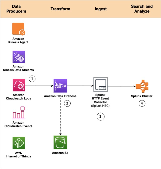
By using a managed service like Amazon Data Firehose for data ingestion into Splunk, we provide out-of-the-box reliability and scalability. One of the pain points of the old approach was the overhead of managing the data collection nodes (Splunk heavy forwarders). With the new Amazon Data Firehose to Splunk integration, there are no forwarders to manage or set up. Data producers (1) are configured through the AWS Management Console to drop data into Amazon Data Firehose.

You can also create your own data producers. For example, you can drop data into a Firehose delivery stream by using Amazon Kinesis Agent, or by using the Firehose API (PutRecord(), PutRecordBatch()), or by writing to a Kinesis Data Stream configured to be the data source of a Firehose delivery stream. For more details, refer to Sending Data to an Amazon Data Firehose Delivery Stream.

You might need to transform the data before it goes into Splunk for analysis. For example, you might want to enrich it or filter or anonymize sensitive data. You can do so using AWS Lambda and enabling data transformation in Amazon Data Firehose. In this scenario, Amazon Data Firehose is used to decompress the Amazon CloudWatch logs by enabling the feature.

Systems fail all the time. Let’s see how this integration handles outside failures to guarantee data durability. In cases when Amazon Data Firehose can’t deliver data to the Splunk Cluster, data is automatically backed up to an S3 bucket. You can configure this feature while creating the Firehose delivery stream (2). You can choose to back up all data or only the data that’s failed during delivery to Splunk.

In addition to using S3 for data backup, this Firehose integration with Splunk supports Splunk Indexer Acknowledgments to guarantee event delivery. This feature is configured on Splunk’s HTTP Event Collector (HEC) (3). It ensures that HEC returns an acknowledgment to Amazon Data Firehose only after data has been indexed and is available in the Splunk cluster (4).

Now let’s look at a hands-on exercise that shows how to forward VPC flow logs to Splunk.

How-to guide

To process VPC flow logs, we implement the following architecture.
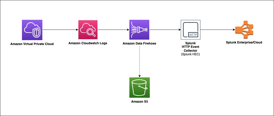
Amazon Virtual Private Cloud (Amazon VPC) delivers flow log files into an Amazon CloudWatch Logs group. Using a CloudWatch Logs subscription filter, we set up real-time delivery of CloudWatch Logs to an Amazon Data Firehose stream.

Data coming from CloudWatch Logs is compressed with gzip compression. To work with this compression, we will enable decompression for the Firehose stream. Firehose then delivers the raw logs to the Splunk Http Event Collector (HEC).

If delivery to the Splunk HEC fails, Firehose deposits the logs into an Amazon S3 bucket. You can then ingest the events from S3 using an alternate mechanism such as a Lambda function.

When data reaches Splunk (Enterprise or Cloud), Splunk parsing configurations (packaged in the Splunk Add-on for Amazon Data Firehose) extract and parse all fields. They make data ready for querying and visualization using Splunk Enterprise and Splunk Cloud.

Walkthrough

Install the Splunk Add-on for Amazon Data Firehose

The Splunk Add-on for Amazon Data Firehose enables Splunk (be it Splunk Enterprise, Splunk App for AWS, or Splunk Enterprise Security) to use data ingested from Amazon Data Firehose. Install the Add-on on all the indexers with an HTTP Event Collector (HEC). The Add-on is available for download from Splunkbase. For troubleshooting assistance, please refer to: AWS Data Firehose troubleshooting documentation & Splunk’s official troubleshooting guide

HTTP Event Collector (HEC)

Before you can use Amazon Data Firehose to deliver data to Splunk, set up the Splunk HEC to receive the data. From Splunk web, go to the Setting menu, choose Data Inputs, and choose HTTP Event Collector. Choose Global Settings, ensure All tokens is enabled, and then choose Save. Then choose New Token to create a new HEC endpoint and token. When you create a new token, make sure that Enable indexer acknowledgment is checked.
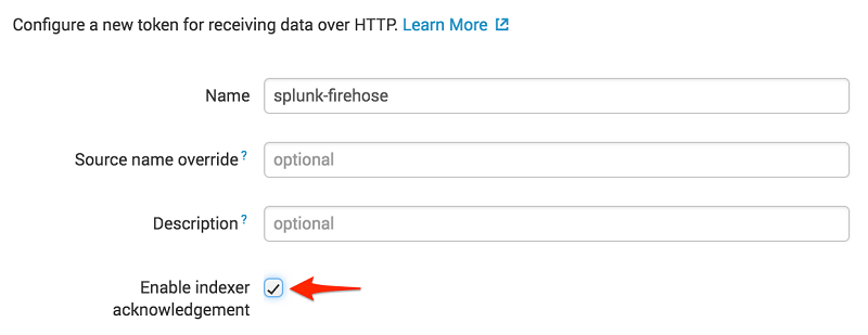
When prompted to select a source type, select aws:cloudwatchlogs:vpcflow

Create an S3 backsplash bucket

To provide for situations in which Amazon Data Firehose can’t deliver data to the Splunk Cluster, we use an S3 bucket to back up the data. You can configure this feature to back up all data or only the data that’s failed during delivery to Splunk.

Note: Bucket names are unique.

aws s3 create-bucket --bucket <your-s3-bucket-name> --create-bucket-configuration LocationConstraint=<your-region>

Create an Amazon Data Firehose delivery stream

On the AWS console, open the Amazon Data Firehose console, and choose Create Firehose Stream.

Select DirectPUT as the source and Splunk as the destination.
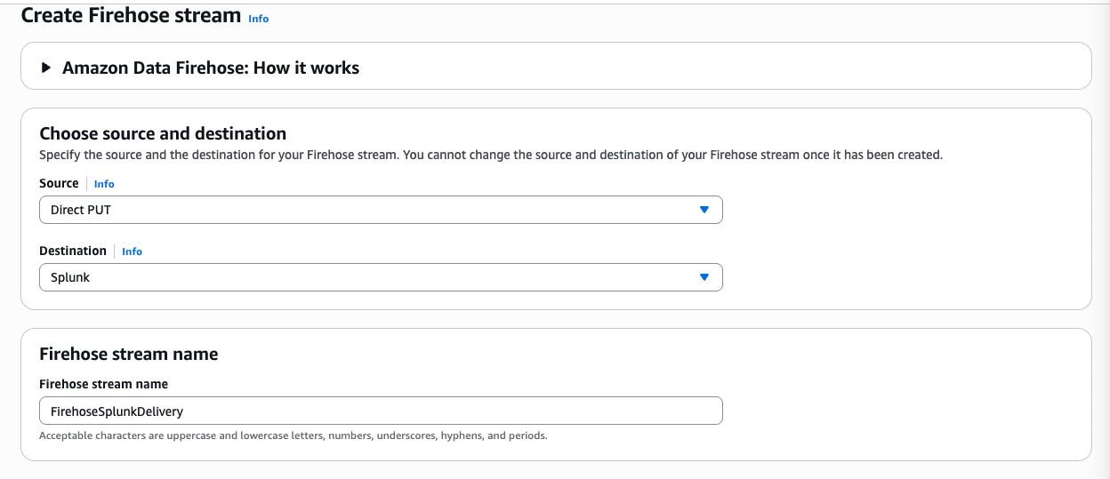
Create Firehose Stream

If you are using Firehose to deliver CloudWatch Logs and want to deliver decompressed data to your Firehose stream destination, use Firehose Data Format Conversion (Parquet, ORC) or Dynamic partitioning. You must enable decompression for your Firehose stream, check out Deliver decompressed Amazon CloudWatch Logs to Amazon S3 and Splunk using Amazon Data Firehose

Enter your Splunk HTTP Event Collector (HEC) information in destination settings
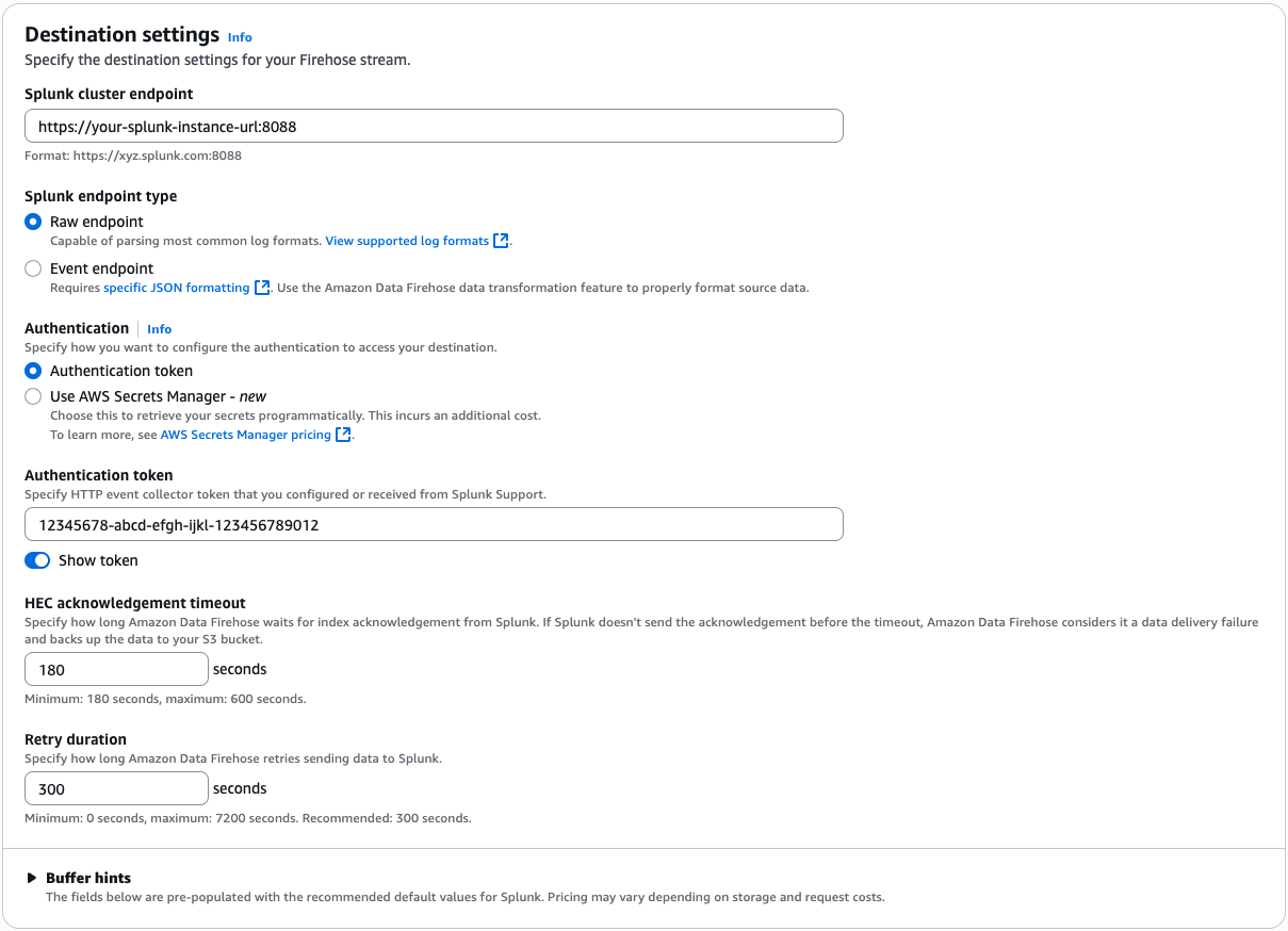
Firehose Destination setting

Note: Amazon Data Firehose requires the Splunk HTTP Event Collector (HEC) endpoint to be terminated with a valid CA-signed certificate matching the DNS hostname used to connect to your HEC endpoint. You receive delivery errors if you are using a self-signed certificate.

In this example, we only back up logs that fail during delivery.
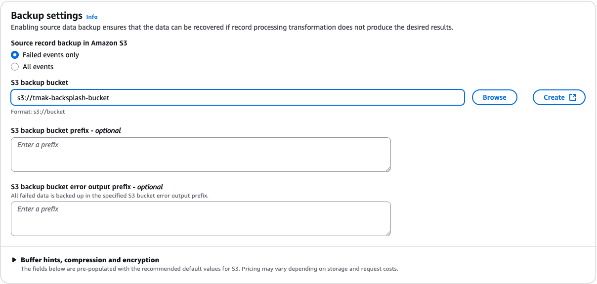
Backsplash S3 settings

To monitor your Firehose delivery stream, enable error logging. Doing this means that you can monitor record delivery errors. Create an IAM role for the Firehose stream by choosing Create new, or Choose existing IAM role.
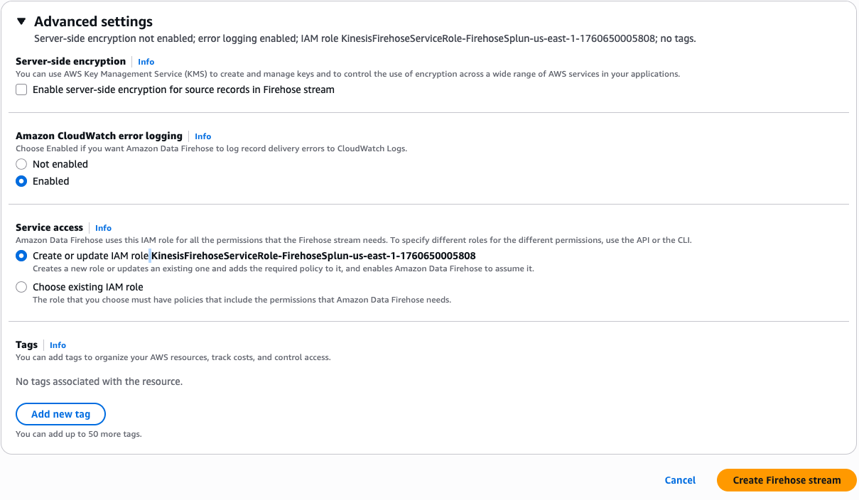
Advance settings for cloudwatch loggings

You now get a chance to review and adjust the Firehose stream settings. When you are satisfied, choose Create Firehose Stream.

Create a VPC Flow Log

To send events from Amazon VPC, you need to set up a VPC flow log. If you already have a VPC flow log you want to use, you can skip to the “Publish CloudWatch to Amazon Data Firehose” section.

On the AWS console, open the Amazon VPC service. Then choose VPC, and choose the VPC you want to send flow logs from. Choose Flow Logs, and then choose Create Flow Log. If you don’t have an IAM role that allows your VPC to publish logs to CloudWatch, choose Create and use a new service role.
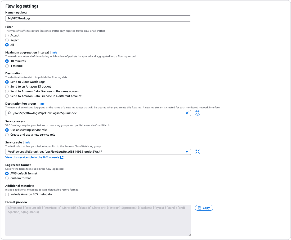
VPC Flow Logs Settings

Once active, your VPC flow log should look like the following.

Flow logs

Publish CloudWatch to Amazon Data Firehose

When you generate traffic to or from your VPC, the log group is created in Amazon CloudWatch. We create an IAM role to allow Cloudwatch to publish logs to the Amazon Data Firehose Stream.

To allow CloudWatch to publish to your Firehose stream, you need to give it permissions.

$ aws iam create-role --role-name CWLtoFirehoseRole --assume-role-policy-document file://TrustPolicyForCWLToFireHose.json


Here is the content for TrustPolicyForCWLToFireHose.json.

{
  "Statement": {
    "Effect": "Allow",
    "Principal": { "Service": "logs.us-east-1.amazonaws.com" },
    "Action": "sts:AssumeRole"
  }
}

Attach the policy to the newly created role.

$ aws iam put-role-policy 
    --role-name CWLtoFirehoseRole 
    --policy-name Permissions-Policy-For-CWL 
    --policy-document file://PermissionPolicyForCWLToFireHose.json

Here is the content for PermissionPolicyForCWLToFireHose.json.

{
    "Statement":[
      {
        "Effect":"Allow",
        "Action":["firehose:*"],
        "Resource":["arn:aws:firehose:us-east-1:YOUR-AWS-ACCT-NUM:deliverystream/FirehoseSplunkDeliveryStream"]
      },
      {
        "Effect":"Allow",
        "Action":["iam:PassRole"],
        "Resource":["arn:aws:iam::YOUR-AWS-ACCT-NUM:role/CWLtoFirehoseRole"]
      }
    ]
}

The new log group has no subscription filter, so set up a subscription filter. Setting this up establishes a real-time data feed from the log group to your Firehose delivery stream. Select the VPC flow log and choose Actions. Then choose Subscription filters followed by Create Amazon Data Firehose subscription filter.
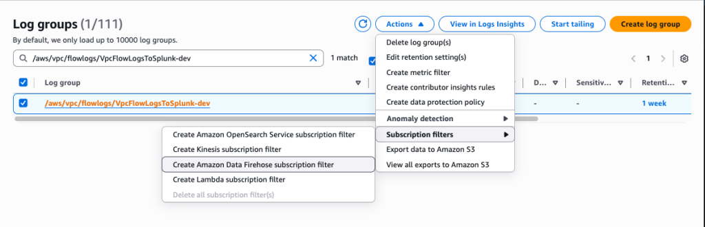
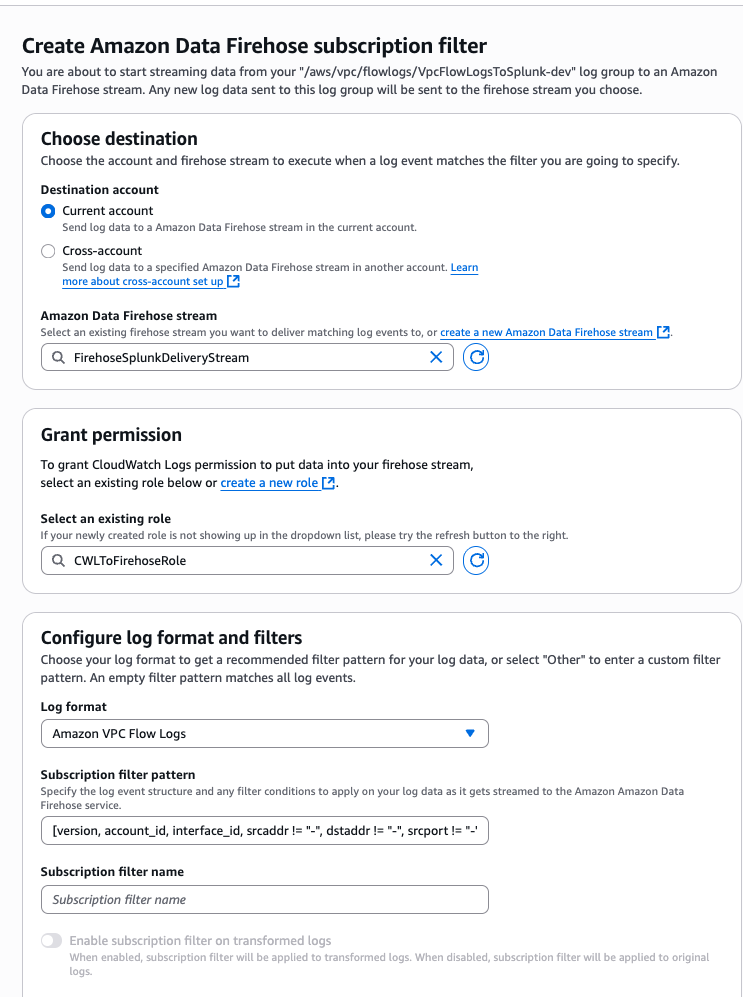
Subscription Filter option

Subscription filter details

When you run the AWS CLI command preceding, you don’t get any acknowledgment. To validate that your CloudWatch Log Group is subscribed to your Firehose stream, check the CloudWatch console.

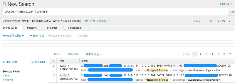
As soon as the subscription filter is created, the real-time log data from the log group goes into your Firehose delivery stream. Your stream then delivers it to your Splunk Enterprise or Splunk Cloud environment for querying and visualization. The screenshot following is from Splunk Enterprise.
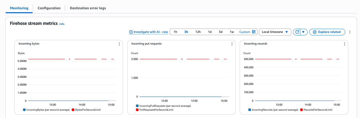
In addition, you can monitor and view metrics associated with your delivery stream using the AWS console.
Conclusion

Although our walkthrough uses VPC Flow Logs, the pattern can be used in many other scenarios. These include ingesting data from AWS IoT, other CloudWatch logs and events, Kinesis Streams or other data sources using the Kinesis Agent or Kinesis Producer Library. You may use a Lambda blueprint or disable record transformation entirely depending on your use case. For an additional use case using Amazon Data Firehose, check out This is My Architecture Video, which discusses how to securely centralize cross-account data analytics using Kinesis and Splunk.

If you found this post useful, be sure to check out Integrating Splunk with Amazon Kinesis Streams.


About the Authors

Tarik Makota

Tarik Makota

Tarik is a solutions architect with the Amazon Web Services Partner Network. He provides technical guidance, design advice and thought leadership to AWS’ most strategic software partners. His career includes work in an extremely broad software development and architecture roles across ERP, financial printing, benefit delivery and administration and financial services. He holds an M.S. in Software Development and Management from Rochester Institute of Technology.

Roy Arsan

Roy Arsan

Roy is a solutions architect in the Splunk Partner Integrations team. He has a background in product development, cloud architecture, and building consumer and enterprise cloud applications. More recently, he has architected Splunk solutions on major cloud providers, including an AWS Quick Start for Splunk that enables AWS users to easily deploy distributed Splunk Enterprise straight from their AWS console. He’s also the co-author of the AWS Lambda blueprints for Splunk. He holds an M.S. in Computer Science Engineering from the University of Michigan.

Yashika Jain

Yashika Jain

Yashika is a Senior Cloud Analytics Engineer at AWS, specializing in real-time analytics and event-driven architectures. She is committed to helping customers by providing deep technical guidance, driving best practices across real-time data platforms and solving complex issues related to their streaming data architectures.

Mitali Sheth

Mitali Sheth

Mitali is a Streaming Data Engineer in the AWS Professional Services team, specializing in real-time analytics and event-driven architectures for AWS’ most strategic software customers. More recently, she has focused on data governance with AWS Lake Formation, building reliable data pipelines with AWS Glue, and modernizing streaming infrastructure with Amazon MSK and Amazon Managed Flink for large-scale enterprise deployments. She holds an M.S. in Computer Science from the University of Florida.

Best practices for querying Apache Iceberg data with Amazon Redshift

Post Syndicated from Anusha Challa original https://aws.amazon.com/blogs/big-data/best-practices-for-querying-apache-iceberg-data-with-amazon-redshift/

Apache Iceberg is an open table format that helps combine the benefits of using both data warehouse and data lake architectures, giving you choice and flexibility for how you store and access data. See Using Apache Iceberg on AWS for a deeper dive on using AWS Analytics services for managing your Apache Iceberg data. Amazon Redshift supports querying Iceberg tables directly, whether they’re fully-managed using Amazon S3 Tables or self-managed in Amazon S3. Understanding best practices for how to architect, store, and query Iceberg tables with Redshift helps you meet your price and performance targets for your analytical workloads.

In this post, we discuss the best practices that you can follow while querying Apache Iceberg data with Amazon Redshift

1. Follow the table design best practices

Selecting the right data types for Iceberg tables is important for efficient query performance and maintaining data integrity. It is important to match the data types of the columns to the nature of the data they store, rather than using generic or overly broad data types.

Why follow table design best practices?

  • Optimized Storage and Performance: By using the most appropriate data types, you can reduce the amount of storage required for the table and improve query performance. For example, using the DATE data type for date columns instead of a STRING or TIMESTAMP type can reduce the storage footprint and improve the efficiency of date-based operations.
  • Improved Join Performance: The data types used for columns participating in joins can impact query performance. Certain data types, such as numeric types (such as, INTEGER, BIGINT, DECIMAL), are generally more efficient for join operations compared to string-based types (such as, VARCHAR, TEXT). This is because numeric types can be easily compared and sorted, leading to more efficient hash-based join algorithms.
  • Data Integrity and Consistency: Choosing the correct data types helps with data integrity by enforcing the appropriate constraints and validations. This reduces the risk of data corruption or unexpected behavior, especially when data is ingested from multiple sources.

How to follow table design best practices?

  • Leverage Iceberg Type Mapping: Iceberg has built-in type mapping that translates between different data sources and the Iceberg table’s schema. Understand how Iceberg handles type conversions and use this knowledge to define the most appropriate data types for your use case.
  • Select the smallest possible data type that can accommodate your data. For example, use INT instead of BIGINT if the values fit within the integer range, or SMALLINT if they fit even smaller ranges.
  • Utilize fixed-length data types when data length is consistent. This can help with predictable and faster performance.
  • Choose character types like VARCHAR or TEXT for text, prioritizing VARCHAR with an appropriate length for efficiency. Avoid over-allocating VARCHAR lengths, which can waste space and slow down operations.
  • Match numeric precision to your actual requirements. Using unnecessarily high precision (such as, DECIMAL(38,20) instead of DECIMAL(10,2) for currency) demands more storage and processing, leading to slower query execution times for calculations and comparisons.
  • Employ date and time data types (such as, DATE, TIMESTAMP) rather than storing dates as text or numbers. This optimizes storage and allows for efficient temporal filtering and operations.
  • Opt for boolean values (such as, BOOLEAN) instead of using integers to represent true/false states. This saves space and potentially enhances processing speed.
  • If the column will be used in join operations, favor data types that are typically used for indexing. Integers and date/time types generally allow for faster searching and sorting than larger, less efficient types like VARCHAR(MAX).

2. Partition your Apache Iceberg table on columns that are most frequently used in filters

When working with Apache Iceberg tables in conjunction with Amazon Redshift, one of the most effective ways to optimize query performance is to partition your data strategically. The key principle is to partition your Iceberg table based on columns that are most frequently used in query filters. This approach can significantly improve query efficiency and reduce the amount of data scanned, leading to faster query execution and lower costs.

Why partitioning Iceberg tables matters?

  • Improved Query Performance: When you partition on columns commonly used in WHERE clauses, Amazon Redshift can eliminate irrelevant partitions, reducing the amount of data it needs to scan. For example, if you have a sales table partitioned by date and you run a query to analyze sales data for January 2024, Amazon Redshift will only scan the January 2024 partition instead of the entire table. This partition pruning can dramatically improve query performance—in this scenario, if you have five years of sales data, scanning just one month means examining only 1.67% of the total data, potentially reducing query execution time from minutes to seconds.
  • Reduced Scan Costs: By scanning less data, you can lower the computational resources required and, consequently the associated costs.
  • Better Data Organization: Logical partitioning helps in organizing data in a way that aligns with common query patterns, making data retrieval more intuitive and efficient.

How to partition Iceberg tables?

  • Analyze your workload to determine which columns are most frequently used in filter conditions. For example, if you always filter your data for the last 6months, then that date will be a good partition key.
  • Select columns that have high cardinality but not too high to avoid creating too many small partitions. Good candidates often include:
    • Date or timestamp columns (such as, year, month, day)
    • Categorical columns with a moderate number of distinct values (such as, region, product category)
  • Define Partition Strategy: Use Iceberg’s partitioning capabilities to define your strategy. For example if you are using Amazon Athena to create a partitioned Iceberg table, you can use the following syntax.
CREATE TABLE [db_name.]table_name (col_name data_type [COMMENT col_comment] [, …]
[PARTITIONED BY (col_name | transform, … )]
LOCATION 's3://amzn-s3-demo-bucket/your-folder/'
TBLPROPERTIES ( 'table_type' = 'ICEBERG' [, property_name=property_value] )

Example

CREATE TABLE iceberg_db.my_table ( id INT, date DATE, region STRING, sales DECIMAL(10,2) )
PARTITIONED BY (date, region)
LOCATION 's3://amzn-s3-demo-bucket/your-folder/'
TBLPROPERTIES ( 'table_type' = 'ICEBERG' )
  • Ensure your Redshift queries take advantage of the partitioning scheme by including partition columns in the WHERE clause whenever possible.

Walk-through with a sample usecase
Let’s take an example to understand how to pick the best partition key by following best practices. Consider an e-commerce company looking to optimize their sales data analysis using Apache Iceberg tables with Amazon Redshift. The company maintains a table called sales_transactions, which has data for 5 years across four regions (North America, Europe, Asia, and Australia) with five product categories (Electronics, Clothing, Home & Garden, Books, and Toys). The dataset includes key columns such as transaction_id, transaction_date, customer_id, product_id, product_category, region, and sale_amount.

The data science team uses transaction_date and region columns frequently in filters, while product_category is used less frequently. The transaction_date column has high cardinality (one value per day), region has low cardinality (only 4 distinct values) and product_category has moderate cardinality (5 distinct values).

Based on this analysis, an effective partition strategy would be to partition by year and month from the transaction_date, and by region. This creates a manageable number of partitions while improving the most common query patterns. Here’s how we could implement this strategy using Amazon Athena:

CREATE TABLE iceberg_db.sales_transactions ( transaction_id STRING, transaction_date DATE, customer_id STRING, product_id STRING, product_category STRING, region STRING, sale_amount DECIMAL(10,2))
PARTITIONED BY (transaction_date, region)
LOCATION 's3://athena-371178653860-22hcl401/sales-data/'
TBLPROPERTIES ('table_type' = 'ICEBERG');

3. Optimize by selecting only the necessary columns for query

Another best practice for working with Iceberg tables is to only select the columns that are necessary for a given query, and to avoid using the SELECT * syntax.

Why should you select only necessary columns?

  • Improved Query Performance: In analytics workloads, users typically analyze subsets of data, performing large-scale aggregations or trend analyses. To optimize these operations, analytics storage systems and file formats are designed for efficient column-based reading. Examples include columnar open file formats like Apache Parquet and columnar databases such as Amazon Redshift. A key best practice to select only the required columns in your queries, so the query engine can reduce the amount of data that needs to be processed, scanned, and returned. This can lead to significantly faster query execution times, especially for large tables.
  • Reduced Resource Utilization: Fetching unnecessary columns consumes additional system resources, such as CPU, memory, and network bandwidth. Limiting the columns selected can help optimize resource utilization and improve the overall efficiency of the data processing pipeline.
  • Lower Data Transfer Costs: When querying Iceberg tables stored in cloud storage (e.g., Amazon S3), the amount of data transferred from the storage service to the query engine can directly impact the data transfer costs. Selecting only the required columns can help minimize these costs.
  • Better Data Locality: Iceberg partitions data based on the values in the partition columns. By selecting only the necessary columns, the query engine can better leverage the partitioning scheme to improve data locality and reduce the amount of data that needs to be scanned.

How to only select necessary columns?

  • Identify the Columns Needed: Carefully analyze the requirements of each query and determine the minimum set of columns required to fulfill the query’s purpose.
  • Use Selective Column Names: In the SELECT clause of your SQL queries, explicitly list the column names you need, rather than using SELECT *.

4. Generate AWS Glue data catalog column level statistics

Table statistics play an important role in database systems that utilize Cost-Based Optimizers (CBOs), such as Amazon Redshift. They help the CBO make informed decisions about query execution plans. When a query is submitted to Amazon Redshift, the CBO evaluates multiple possible execution plans and estimates their costs. These cost estimates heavily depend on accurate statistics about the data, including: Table size (number of rows), column value distributions, Number of distinct values in columns, Data skew information, and more.

AWS Glue Data Catalog supports generating statistics for data stored in the data lake including for Apache Iceberg. The statistics include metadata about the columns in a table, such as minimum value, maximum value, total null values, total distinct values, average length of values, and total occurrences of true values. These column-level statistics provide valuable metadata that helps optimize query performance and improve cost efficiency when working with Apache Iceberg tables.

Why generating AWS Glue statistics matter?

  • Amazon Redshift can generate better query plans using column statistics, thereby improve performance on queries due to optimized join orders, better predicate push-down and more accurate resource allocation.
  • Costs will be optimized. Better execution plans lead to reduced data scanning, more efficient resource utilization and overall lower query costs.

How to generate AWS Glue statistics?

The Sagemaker Lakehouse Catalog enables you to generate statistics automatically for updated and created tables with a one-time catalog configuration. As new tables are created, the number of distinct values (NDVs) are collected for Iceberg tables. By default, the Data Catalog generates and updates column statistics for all columns in the tables on a weekly basis. This job analyzes 50% of records in the tables to calculate statistics.

  • On the Lake Formation console, choose Catalogs in the navigation pane.
  • Select the catalog that you want to configure, and choose Edit on the Actions menu.
  • Select Enable automatic statistics generation for the tables of the catalog and choose an IAM role. For the required permissions, see Prerequisites for generating column statistics.
  • Choose Submit.

You can override the defaults and customize statistics collection at the table level to meet specific needs. For frequently updated tables, statistics can be refreshed more often than weekly. You can also specify target columns to focus on those most commonly queried. You can set what percentage of table records to use when calculating statistics. Therefore, you can increase this percentage for tables that need more precise statistics, or decrease it for tables where a smaller sample is sufficient to optimize costs and statistics generation performance.These table-level settings can override the catalog-level settings previously described.

Read the blog Introducing AWS Glue Data Catalog automation for table statistics collection for improved query performance on Amazon Redshift and Amazon Athena for more information.

5. Implement Table Maintenance Strategies for Optimal Performance

Over time, Apache Iceberg tables can accumulate various types of metadata and file artifacts that impact query performance and storage efficiency. Understanding and managing these artifacts is crucial for maintaining optimal performance of your data lake. As you use Iceberg tables, three main types of artifacts accumulate:

  • Small Files: When data is ingested into Iceberg tables, especially through streaming or frequent small batch updates, many small files can accumulate because each write operation typically creates new files rather than appending to existing ones.
  • Deleted Data Artifacts: Iceberg uses copy-on-write for updates and deletes. When records are deleted, Iceberg creates “delete markers” rather than immediately removing the data. These markers need to be processed during reads to filter out deleted records.
  • Snapshots: Every time you make changes to your table (insert, update, or delete data), Iceberg creates a new snapshot—essentially a point-in-time view of your table. While valuable for maintaining history, these snapshots increase metadata size over time, impacting query planning and execution.
  • Unreferenced Files: These are files that exist in storage but aren’t linked to any current table snapshot. They occur in two main scenarios:
    1. When old snapshots are expired, the files exclusively referenced by those snapshots become unreferenced
    2. When write operations are interrupted or fail midway, creating data files that aren’t properly linked to any snapshot

Why table maintenance matters?

Regular table maintenance delivers several important benefits:

  • Enhanced Query Performance: Consolidating small files reduces the number of file operations required during queries, while removing excess snapshots and delete markers streamlines metadata processing. These optimizations allow query engines to access and process data more efficiently.
  • Optimized Storage Utilization: Expiring old snapshots and removing unreferenced files frees up valuable storage space, helping you maintain cost-effective storage utilization as your data lake grows.
  • Improved Resource Efficiency: Maintaining well-organized tables with optimized file sizes and clean metadata requires less computational resources for query execution, allowing your analytics workloads to run faster and more efficiently.
  • Better Scalability: Properly maintained tables scale more effectively as data volumes grow, maintaining consistent performance characteristics even as your data lake expands.

How to perform table maintenance?

Three key maintenance operations help optimize Iceberg tables:

  1. Compaction: Combines smaller files into larger ones and merges delete files with data files, resulting in streamlined data access patterns and improved query performance.
  2. Snapshot Expiration: Removes old snapshots that are no longer needed while maintaining a configurable history window.
  3. Unreferenced File Removal: Identifies and removes files that are no longer referenced by any snapshot, reclaiming storage space and reducing the total number of objects the system needs to track.

AWS offers a fully managed Apache Iceberg data lake solution called S3 tables that automatically takes care of table maintenance, including:

  • Automatic Compaction: S3 Tables automatically perform compaction by combining multiple smaller objects into fewer, larger objects to improve Apache Iceberg query performance. When combining objects, compaction also applies the effects of row-level deletes in your table. You can manage compaction process based on the configurable table level properties.
    • targetFileSizeMB: Default is 512 MB. Can be configured to a value between between 64 MiB and 512 MiB.

Apache Iceberg offers various methods like Binpack, Sort, Z-order to compact data. By default Amazon S3 selects the best of these three compaction strategy automatically based on your table sort order

  • Automated Snapshot Management: S3 Tables automatically expires older snapshots based on configurable table level properties
    • MinimumSnapshots (1 by default): Minimum number of table snapshots that S3 Tables will retain
    • MaximumSnapshotAge (120 hours by default): This parameter determines the maximum age, in hours, for snapshots to be retained
  • Unreferenced File Removal: Automatically identifies and deletes objects not referenced by any table snapshots based on configurable bucket level properties:
    • unreferencedDays (3 days by default): Objects not referenced for this duration are marked as noncurrent
    • nonCurrentDays (10 days by default): Noncurrent objects are deleted after this duration

Note: Deletes of noncurrent objects are permanent with no way to recover these objects.

If you are managing Iceberg tables yourself, you’ll need to implement these maintenance tasks:

Using Athena:
  • Run OPTIMIZE command using the following syntax:
    OPTIMIZE [database_name.]<table_name>;

    This command triggers the compaction process, which utilizes a bin-packing algorithm to group small data files into larger ones. It also merges delete files with existing data files, effectively cleaning up the table and improving its structure.

  • Set the following table properties during iceberg table creation: vacuum_min_snapshots_to_keep (Default 1): Minimum snapshots to retain vacuum_max_snapshot_age_seconds (Default 432000 seconds or 5 days)
  • Periodically run the VACUUM command to expire old snapshots and remove unreferenced files. Recommended after performing operations like merge on iceberg tables. Syntax: VACUUM [database_name.]target_table. VACUUM performs snapshot expiration and orphan file removal
Using Spark SQL:
  • Schedule regular compaction jobs with Iceberg’s rewrite files action
  • Use expireSnapshots operation to remove old snapshots
  • Run deleteOrphanFiles operation to clean up unreferenced files
  • Establish a maintenance schedule based on your write patterns (hourly, daily, weekly)
  • Run these operations in sequence, typically compaction followed by snapshot expiration and unreferenced file removal
  • It’s especially important to run these operations after large ingest jobs, heavy delete operations, or overwrite operations

6. Create incremental materialized views on Apache Iceberg tables in Redshift to improve performance of time sensitive dashboard queries

Organizations across industries rely on data lake powered dashboards for time-sensitive metrics like sales trends, product performance, regional comparisons, and inventory rates. With underlying Iceberg tables containing billions of records and growing by millions daily, recalculating metrics from scratch during each dashboard refresh creates significant latency and degrades user experience.

The integration between Apache Iceberg and Amazon Redshift enables creating incremental materialized views on Iceberg tables to optimize dashboard query performance. These views enhance efficiency by:

  • Pre-computing and storing complex query results
  • Using incremental maintenance to process only recent changes since last refresh
  • Reducing compute and storage costs compared to full recalculations

Why incremental materialized views on Iceberg tables matter?

  • Performance Optimization: Pre-computed materialized views significantly accelerate dashboard queries, especially when accessing large-scale Iceberg tables
  • Cost Efficiency: Incremental maintenance through Amazon Redshift processes only recent changes, avoiding expensive full recomputation cycles
  • Customization: Views can be tailored to specific dashboard requirements, optimizing data access patterns and reducing processing overhead

How to create incremental materialized views?

  • Determine which Iceberg tables are the primary data sources for your time-sensitive dashboard queries.
  • Use the CREATE MATERIALIZED VIEW statement to define the materialized views on the Iceberg tables. Ensure that the materialized view definition includes only the necessary columns and any applicable aggregations or transformations.
  • If you have used all operators that are eligible for an incremental refresh, Amazon Redshift automatically creates an incrementally refresh-able materialized view. Refer to limitations for incremental refresh to understand the operations that are not eligible for an incremental refresh
  • Regularly refresh the materialized views using REFRESH MATERIALIZED VIEW command

7. Create Late binding views (LBVs) on Iceberg table to encapsulate business logic.

Amazon Redshift’s support for late binding views on external tables, including Apache Iceberg tables, allows you to encapsulate your business logic within the view definition. This best practice provides several benefits when working with Iceberg tables in Redshift.

Why create LBVs?

  • Centralized Business Logic: By defining the business logic in the view, you can ensure that the transformation, aggregation, and other processing steps are consistently applied across all queries that reference the view. This promotes code reuse and maintainability.
  • Abstraction from Underlying Data: Late binding views decouple the view definition from the underlying Iceberg table structure. This allows you to make changes to the Iceberg table, such as adding or removing columns, without having to update the view definitions that depend on the table.
  • Improved Query Performance: Redshift can optimize the execution of queries against late binding views, leveraging techniques like predicate pushdown and partition pruning to minimize the amount of data that needs to be processed.
  • Enhanced Data Security: By defining access controls and permissions at the view level, you can grant users access to only the data and functionality they require, improving the overall security of your data environment.

How to create LBVs?

  • Identify suitable Apache Iceberg tables: Determine which Iceberg tables are the primary data sources for your business logic and reporting requirements.
  • Create late binding views(LBVs): Use the CREATE VIEW statement to define the late binding views on the external Iceberg tables. Incorporate the necessary transformations, aggregations, and other business logic within the view definition.
    Example:

    CREATE VIEW my_iceberg_view AS
    SELECT col1,col2,SUM(col3) AS total_col3
    GROUP BY col1, col2
    WITH NO SCHEMA BINDING;
    

  • Grant View Permissions: Assign the appropriate permissions to the views, granting access to the users or roles that require access to the encapsulated business logic.

Conclusion

In this post, we covered best practices for using Amazon Redshift to query Apache Iceberg tables, focusing on fundamental design decisions. One key area is table design and data type selection, as this can have the greatest impact on your storage size and query performance. Additionally, using Amazon S3 Tables to have a fully-managed tables automatically handle essential maintenance tasks like compaction, snapshot management, and vacuum operations, allowing you to focus building your analytical applications.

As you build out your workflows to use Amazon Redshift with Apache Iceberg tables, considering the following best practices to help you achieve your workload goals:

  • Adopting Amazon S3 Tables for new implementations to leverage automated management features
  • Auditing existing table designs to identify opportunities for optimization
  • Developing a clear partitioning strategy based on actual query patterns
  • For self-managed Apache Iceberg tables on Amazon S3, implementing automated maintenance procedures for statistics generation and compaction


About the authors

Anusha Challa

Anusha Challa

Anusha is a Senior Analytics Specialist Solutions Architect focused on Amazon Redshift. She has helped 100s of customers build large-scale analytics solutions in the cloud and on premises. She is passionate about data analytics, data science and AI.

Mohammed Alkateb

Mohammed Alkateb

Mohammed is an Engineering Manager at Amazon Redshift. Mohammed has 18 US patents, and he has publications in research and industrial tracks of premier database conferences including EDBT, ICDE, SIGMOD and VLDB. Mohammed holds a PhD in Computer Science from The University of Vermont, and MSc and BSc degrees in Information Systems from Cairo University.

Jonathan Katz

Jonathan Katz

Jonathan is a Core Team member of the open source PostgreSQL project and an active open source contributor.

IPv6 addressing with Amazon Redshift

Post Syndicated from Srini Ponnada original https://aws.amazon.com/blogs/big-data/ipv6-addressing-with-amazon-redshift/

As we witness the gradual transition from IPv4 to IPv6, Amazon Web Services (AWS) continues to expand its support for dual-stack networking across its service portfolio. In this post, we show how you can migrate your Amazon Redshift Serverless workgroup from IPv4-only to dual-stack mode, so you can make your data warehouse future ready.

An IP address serves as a digital identity for devices connected to the internet. This unique numerical identifier enables devices to communicate across IP-based networks, facilitating the exchange of data packets between source and destination.

Today’s internet operates on two IP versions:

  • IPv4 – The traditional 32-bit addressing system (such as 192.168.0.22) that has powered internet communications for over three decades. With approximately 4 billion possible addresses (2³²), IPv4’s limitations have become increasingly apparent as our digital environment expands.
  • IPv6 – The next-generation 128-bit addressing system (such as 2606:4700::6810:787f) offers an astronomical number of unique addresses (340 undecillion or 2¹²⁸). This virtually unlimited address space is designed to accommodate the explosive growth of internet-connected devices.

In the case of Amazon Redshift, dual-stack networking allows Redshift workgroups to communicate over both IPv4 and IPv6 protocols simultaneously. This networking architecture allows Redshift workgroups to be accessible using both IPv4 and IPv6 addresses, providing greater flexibility and future-proofing for network communications. Dual-stack networking provides the following advantages:

  1. Future-proofing – Facilitates compatibility with both IPv4 systems and modern IPv6 networks
  2. Enhanced connectivity – Provides more flexible networking options for diverse client applications

Enable dual-stack networking for Amazon Redshift

An Amazon Redshift workgroup operating in dual-stack mode has both IPv4 and IPv6 addresses associated with the database endpoints. We’ve introduced a new API field called ipAddressTypein the Amazon Redshift API that gives you direct control over your workgroup’s network configuration. You can now specifically choose whether your Amazon Redshift instance operates in IPv4-only mode or dual-stack mode. For complete implementation details, refer to the ipAddressType parameter in the Amazon Redshift API Reference.

Best practice

When implementing dual-stack networking in Amazon Redshift, deploy your workgroups in private subnets with virtual private cloud (VPC) endpoints for optimal security and compatibility. This approach aligns with the current Amazon Redshift support model, which requires dual-stack databases to operate in private mode only. Amazon Redshift doesn’t currently support databases with IPv6-only endpoints or publicly accessible dual-stack instances.

Prerequisites

To implement dual-stack networking in Amazon Redshift, you need to have the following prerequisites:

  • An existing Amazon Redshift serverless workgroups running in IPv4-only mode that you want to convert to dual-stack mode
  • Administrative permissions to modify Amazon Redshift workgroup network configurations
  • VPC with both IPv4 and IPv6 CIDR blocks assigned

Enable IPv6 support in your VPC subnets

Before migrating your Amazon Redshift Serverless workgroup to dual-stack mode, you must first make sure your VPC subnets support IPv6 addressing. In this section, we walk through the process of enabling IPv6 CIDR blocks for your VPC.

Existing VPC Subnets

To enable dual-stack mode in your existing VPC follow these five high-level steps:

  1. Access the VPC dashboard
  2. Navigate to the subnet settings
  3. Add the IPv6 CIDR block
  4. Repeat for the required subnets
  5. Verify IPv6 CIDR association

To access the VPC dashboard:

  1. Sign in to your account on the AWS Management Console
  2. In the search bar at the top, type VPC
  3. Choose VPC from the dropdown list to navigate to the Amazon Virtual Private Cloud (Amazon VPC) dashboard

To navigate to subnet settings:

  1. In the left navigation panel under Virtual private cloud, choose Subnets
  2. From the subnet list, identify and select the subnet(s) that your Amazon Redshift Serverless workgroup uses or will use

To add the IPv6 CIDR block:

  1. With your subnet selected, choose Actions in the dropdown list
  2. Choose Edit IPv6 CIDRs from the available options
  3. In the configuration panel that appears, choose Add IPv6 CIDR
  4. The system will automatically suggest an appropriate IPv6 CIDR block allocation
  5. Choose Save to apply the changes

Repeat for the required subnets. You must modify the subnets within the VPC that will be used by your Amazon Redshift resources. Repeat high-level steps 2–3 for each subnet in your Amazon Redshift subnet group.

Verify the IPv6 CIDR association. After completing the configuration, verify that each subnet displays both IPv4 and IPv6 CIDR blocks in the subnet details. Your subnet details should show something like the following snippet:IPv4 CIDR: 10.0.0.0/24IPv6 CIDR: 2600:1f16:c72:9d00::/64

After you’ve successfully configured IPv6 CIDR blocks for the relevant subnets, you’re ready to proceed with enabling dual-stack mode on your Amazon Redshift Serverless workgroup.

New VPC Subnets

To enable dual-stack mode in a new VPC, follow these steps:

  1. To create a dual-stack VPC, add the --amazon-provided-ipv6-cidr-block option to add an Amazon provided IPv6 CIDR block, as shown in the following example:
    aws ec2 create-vpc --cidr-block 10.0.0.0/24 \
    --amazon-provided-ipv6-cidr-block \
    --query Vpc.VpcId \
    --output text

  2. [Dual stack VPC] Get the IPv6 CIDR block that’s associated with your VPC by using the following describe-vpcs command:
    aws ec2 describe-vpcs --vpc-id vpcxxxxx \
    --query Vpcs[].Ipv6CidrBlockAssociationSet[].Ipv6CidrBlock \
    --output text

  3. If you created a dual-stack VPC, you can use the --ipv6-cidr-block option to create a dual stack subnet, as shown in the following command:
    aws ec2 create-subnet --vpc-id vpc-xxx \
    --cidr-block 10.0.1.0/20 \
    --ipv6-cidr-block 2600:1f13:cfe:3600::/64 \
    --availability-zone us-east-2a \
    --query Subnet.SubnetId \
    --output text

Migrate an existing Amazon Redshift Serverless workgroup from IPv4 to IPv6

To enable dual-stack mode for your Amazon Redshift Serverless workgroup, follow these five high-level steps:

  1. Access Amazon Redshift Serverless
  2. Select your workgroup
  3. Access network and security settings
  4. Enable dual-stack mode
  5. Verify the configuration

To access Amazon Redshift Serverless:

  1. Sign in to AWS Management Console using your credentials.
  2. In the search bar at the top of the console, enter Redshift.
  3. Choose Amazon Redshift in the dropdown list. This will take you to the Amazon Redshift dashboard. Confirm Make sure you’re on the Redshift Serverless dashboard view

To select your workgroup:

  1. In the Redshift Serverless dashboard, locate the Workgroups section
  2. Select the name of the specific workgroup you want to modify

To access network and security settings:

  1. On the workgroup details page, locate the horizontal navigation tabs
  2. Next to the Query and database monitoring section, choose the Data access tab
  3. Choose Edit to access the Edit network and security page

To enable dual-stack mode:

  1. In the network settings section, locate the IP address type options
  2. Choose Dual-stack mode. This enables connectivity for both IPv4 and IPv6
  3. Choose Save changes at the bottom of the page

To verify the configuration:

After the changes are applied, you’ll be returned to the workgroup details page. Confirm that your workgroup now displays Dual-stack mode in its network settings, as shown in the following screenshot.

Your Amazon Redshift Serverless workgroup is now configured to support both IPv4 and IPv6 traffic. This configuration allows your Redshift Serverless workgroup to communicate over both IPv4 and IPv6 protocols, providing greater flexibility for your network connectivity options.

Access Redshift dual-stack serverless workgroups

Redshift dual-stack workgroups maintain the same access methods regardless of whether you’re connecting using IPv4 or IPv6. Your existing connection endpoints remain unchanged.

To access a Redshift dual-stack workgroups from an Amazon Elastic Compute Cloud (Amazon EC2) instance, follow these steps:

  1. Create an IPv4 EC2 instance.
  2. Add the associated EC2 security group to your Redshift workgroup’s security group inbound rules.
  3. Connect to your EC2 instance. Log in to your EC2 instance on the AWS console to install the psql client to test the database connectivity. Enter the following commands from the terminal window:
    # Update your system packages
    sudo dnf update -y
    # Install the PostgreSQL 15 repository
    sudo dnf install -y postgresql15
    # Verify the installation
    psql –version

    Connect to your Redshift workgroup using application user

    psql -h your-redshift-endpoint -U your-username -d your-database -p 5439

    Enter password when prompted

  4. Enter sample queries, as shown in the following:
    SELECT * FROM your_table LIMIT 10;

  5. Validate the IPv4 connection using the following SQL by replacing your associated IPv4 EC2 instance IP address:
    SELECT * FROM sys_connection_log where user_name = 'admin' 
    and remote_host like '%172.31.83.132%' order by record_time desc;

  6. Execute identical validation steps on your IPv6-enabled EC2 instance to verify that all functionality operates correctly with the IPv6 protocol stack using the preceding commands.

Create dual-stack mode in Amazon Redshift Serverless using AWS CLI

You can create a new dual-stack mode in Amazon Redshift Serverless using AWS Command Line Interface (AWS CLI). Follow these high-level steps:

  1. Create a namespace
  2. Create a workgroup
  3. Verify the workgroup is set up in dual-stack mode

To create namespace, enter the following code:

export AWS_USE_DUALSTACK_ENDPOINT=true
aws redshift-serverless create-namespace \
--region us-east-1 \
--namespace-name ipv6-demo \
--admin-username xxx  \
--admin-user-password "yyyyyyy"

To create workgroup, enter the following code:

aws redshift-serverless create-workgroup \
--workgroup-name ipv6-demo-wg \
--namespace-name ipv6-demo \
--region us-east-1 \
--subnet-ids subnet-ppppppp subnet-qqqqqq \
--ip-address-type dualstack

To verify the workgroup is set up in dual-stack mode, refer to the steps in the previous section.

Clean up

To clean up your resources, complete the following steps:

  1. On the Amazon Redshift Serverless console, delete the Amazon Redshift workgroups and namespaces
  2. On the Amazon EC2 console, terminate the EC2 instances

Conclusion

In this post, we’ve explored the capability of Amazon Redshift Serverless to support IPv6 addressing through dual-stack mode, marking a significant advancement in the AWS data warehouse networking flexibility.

We’ve walked through the complete migration journey, from preparing your VPC subnets with IPv6 CIDR blocks to configuring your Amazon Redshift Serverless workgroup for dual-stack operation. The process is straightforward. Although IPv6-only configurations aren’t yet supported for Amazon Redshift, the dual-stack approach provides an ideal transition path, maintaining compatibility with existing IPv4 systems while introducing IPv6 capabilities. Remember that dual-stack configurations are currently limited to private access mode, with public accessibility not yet supported for dual-stack instances.

By migrating to dual-stack mode now, you can make sure your Amazon Redshift environment remains optimally connected, addressable, and ready to support your organization’s data analytics needs well into the future—regardless of how internet addressing protocols continue to evolve.

If you have questions or suggestions on the content covered in this post, leave them in the comments section.


About the authors

Srini Ponnada

Srini Ponnada

Srini is a Sr. Data Architect at AWS. He has helped customers build scalable data warehousing and big data solutions for over 20 years. He loves to design and build efficient end-to-end solutions on AWS.

Ji Yanzhu

Yanzhu Ji

Ji Yanzhu is a Senior Product Manager on the Amazon Redshift team. She has extensive experience in database security and developing product vision and strategy for industry-leading data products and platforms. She excels at building robust software products using web development, system design, database, and distributed programming techniques.

Hua Zirui

Hua Zirui

Zirui Hua is a Software Development Engineer for Amazon Redshift, where he works on developing next generation features for Amazon Redshift. His main focuses are on networking and proxy of database. Outside of work, he likes to play tennis and basketball.

Sandeep Adwankar

Sandeep Adwankar

Sandeep is a Senior Product Manager at AWS. Based in the California Bay Area, he works with customers around the globe to translate business and technical requirements into products that enable customers to improve how they manage, secure, and access data.

Sumanth Punyamurthula

Sumanth Punyamurthula

Sumanth is a Senior Data and Analytics Architect at AWS with more than 20 years of experience in leading large analytical initiatives, including analytics, data warehouse, data lakes, data governance, security, and cloud infrastructure across travel, hospitality, financial, and healthcare industries.

Niranjan Kulkarni

Niranjan Kulkarni

Niranjan is a Software Development Engineer for Amazon Redshift. He focuses on Amazon Redshift Serverless adoption and Amazon Redshift security-related features. Outside of work, he spends time with his family and enjoys watching high-quality TV series.

Asahi Linux 6.18 progress report

Post Syndicated from jzb original https://lwn.net/Articles/1050953/

The Asahi Linux project has published
its progress report following the release of Linux 6.18. This time
around the project reports progress on many fronts, including
microphone support for M2 Pro/Max MacBooks, work queued for Linux 6.19
to support USB3 via the USB-C ports, and work to improve the Asahi
Linux installation experience. The project is also enabling as
additional System Management Controller (SMC) drivers, which means
that “the myriad voltage, current, temperature and power sensors
controlled by the SMC will be readable using the standard hwmon
interfaces
“.

[$] The Civil Infrastructure Platform after (nearly) ten years

Post Syndicated from corbet original https://lwn.net/Articles/1049604/

The Civil Infrastructure Platform
(CIP) first launched in that form in April 2016, so it has a
tenth-anniversary celebration in its near future. At the 2025 Open
Source Summit Japan
, Yoshitake Kobayashi talked about the goals of this
project and where it is headed in the future. Supporting a Linux system
for even one year is a challenging task; maintaining that support for a
decade or more is rather more so, and a changing regulatory environment
complicates the task further.

Security updates for Wednesday

Post Syndicated from jzb original https://lwn.net/Articles/1050942/

Security updates have been issued by Debian (node-url-parse), Fedora (assimp, conda-build, mod_md, util-linux, and webkitgtk), Oracle (firefox), SUSE (chromium, librsvg, poppler, python311, qemu, strongswan, webkit2gtk3, wireshark, and xen), and Ubuntu (linux-azure, linux-azure-5.4, linux-azure-5.15, linux-azure-fips, and linux-raspi, linux-raspi-realtime, linux-xilinx).

Dynamic EASM Discovery: Continuous Discovery for a Changing Attack Surface

Post Syndicated from Ed Montgomery original https://www.rapid7.com/blog/post/pt-dynamic-easm-discovery-continuous-discovery-for-a-changing-attack-surface

Staying ahead of what’s exposed, automatically.

The modern enterprise doesn’t stand still. New domains are registered, acquisitions bring inherited infrastructure, cloud workloads spin up and down daily, and somewhere in the middle of it all, your visible footprint on the internet external attack surface keeps expanding.

For CISOs, this constant motion makes one CTEM step particularly difficult: discovery. You can’t validate what you can’t see and manual inventory updates can’t keep up with the pace of digital change.

That’s why Rapid7 is introducing dynamic EASM discovery for Surface Command, a new capability that automatically identifies and tracks every part of your external attack surface. By continuously ingesting known domain and IP information from your environment and related management tools, Surface Command ensures your visibility is always accurate, always current, and always ready for validation.

easm.jpg

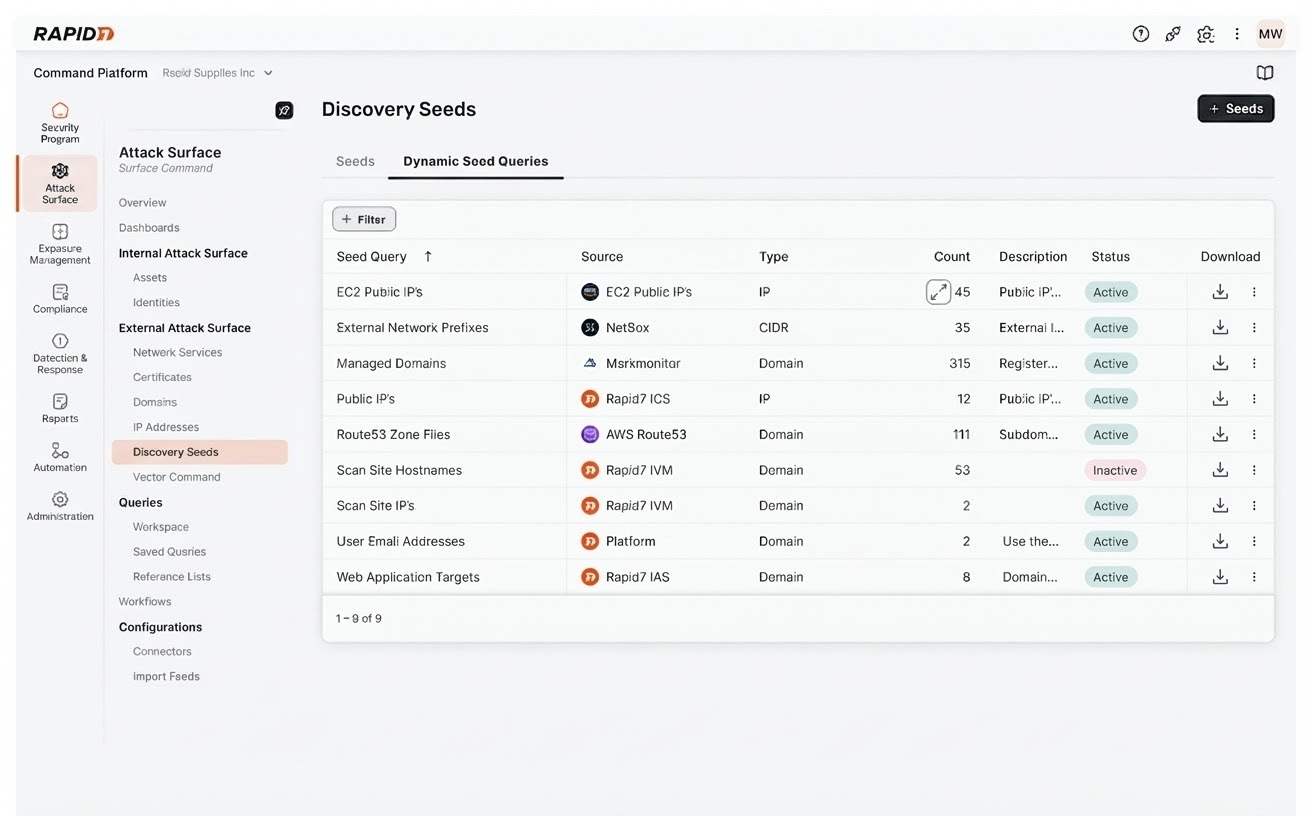
Figure 1: Dynamic Seeds feature in the Rapid7 Command Platform

From static inventories to continuous confidence

Traditional External Attack Surface Management (EASM) tools rely on static “seed lists”, known IPs, domains, or networks used to start discovery scans. But as organizations evolve, those seeds quickly become stale, leaving blind spots that attackers can exploit.

Dynamic EASM discovery replaces static inputs with live intelligence. Surface Command, Rapid7’s attack surface management (ASM) solution, now automatically gathers seed data from across your ecosystem, including DNS records, network services, and asset repositories and feeds it directly into the Rapid7 Command Platform. Asset, vulnerability, automation, control, threat, and enrichment data are ingested into our Command Platform through Connectors.

The result: a continuously updated, validated view of your internet-facing footprint.

No spreadsheets. No manual uploads. No surprises.

Why this matters for CTEM step 2: Discovery

Continuous threat exposure management (CTEM) is the discipline of constantly discovering, prioritizing, validating, and mobilizing against risk. Most organizations excel at discovery and prioritization but validation often lags behind.

Discovery is where confidence becomes measurable:

  • Did the exposure we fixed actually disappear?
  • Is our attack surface shrinking or just shifting?
  • Are we making progress we can prove?

Dynamic EASM discovery strengthens step 2, discovery by ensuring your exposure data reflects the real, live environment. Every time a cloud resource changes or a new asset appears, Surface Command automatically revalidates what’s known versus what’s newly exposed.

That means your CTEM cycle is never out of sync with reality, and your reports to leadership reflect verified reductions in risk, not assumptions.

Connecting visibility to outcomes

Dynamic EASM discovery doesn’t just simplify inventory management, it accelerates progress across the CTEM lifecycle:

  • Discovery: Continuously ingesting data expands your external visibility.
  • Prioritization: Integrated context links assets to business impact and threat intelligence.
  • Validation: Continuous seed refresh confirms exposures are resolved and risk is reducing.
  • Mobilization: Validated insights flow into ITSM and automation workflows for closure.

For security leaders, this translates to clear, measurable progress: a smaller attack surface, shorter exposure windows, and data that executives can trust.

An attacker’s view you can trust

External visibility is only useful if it’s reliable. With dynamic EASM discovery, Surface Command provides a real-time, attacker’s-eye view of your organization’s public-facing assets, domains, subdomains, IPs, and network services; all validated against live data.

This level of automation gives CISOs three distinct advantages:

  • Fewer blind spots – Automatically capture new and transient assets the moment they appear.
  • Proven accuracy – Validate that remediation efforts have actually closed exposures.
  • Faster decisions – Operate on verified intelligence instead of lagging asset data.

Validation becomes continuous, evidence-based, and defensible.

Executive clarity through proof

Boards don’t want more alerts, they want proof that investments in security are paying off. Dynamic EASM Discovery helps CISOs demonstrate that progress with concrete, validated metrics:

  • Total external assets tracked over time
  • Exposure reduction percentages by business unit
  • Remediation velocity measured in real, verified outcomes

When the question comes, “are we actually reducing risk?”

Surface Command gives you evidence, not estimates.

Simplified operations, stronger security

Dynamic EASM discovery is built into Rapid7’s Command Platform, eliminating the manual effort that once slowed exposure management. Security and IT teams can focus on reducing risk instead of reconciling data sources, while automation keeps inventories and dashboards perpetually up to date.

In practice, that means:

  • Reduced administrative overhead
  • Elimination of stale or duplicate records
  • Seamless integration with other Command Platform services for unified CTEM execution

What used to take hours of manual input now happens automatically, at the speed your business evolves.

Continuous validation made simple

Attack surface expansion doesn’t stop, and neither should your visibility. With dynamic EASM discovery, Rapid7 ensures that the foundation of your CTEM program, discovery, is always grounded in current, accurate data.

It’s continuous assurance for a world that doesn’t stand still. This is in early access now, and generally available in January, 2026.

Explore Surface Command

See how Dynamic EASM Discovery keeps your external visibility live, validated, and ready for action.

Contact your Rapid7 account team or click here to initiate a no commitment trial today.

Try the new dynamic EASM discovery self-guided product tour

How did IRC ping timeouts end up in a lawsuit?

Post Syndicated from Matthew Garrett original https://mjg59.dreamwidth.org/73777.html

I recently won a lawsuit against Roy and Rianne Schestowitz, the authors and publishers of the Techrights and Tuxmachines websites. The short version of events is that they were subject to an online harassment campaign, which they incorrectly blamed me for. They responded with a large number of defamatory online posts about me, which the judge described as unsubstantiated character assassination and consequently awarded me significant damages. That’s not what this post is about, as such. It’s about the sole meaningful claim made that tied me to the abuse.

In the defendants’ defence and counterclaim[1], 15.27 asserts in part The facts linking the Claimant to the sock puppet accounts include, on the IRC network: simultaneous dropped connections to the mjg59_ and
elusive_woman accounts. This is so unlikely to be coincidental that the natural inference is that the same person posted under both names
. “elusive_woman” here is an account linked to the harassment, and “mjg59_” is me. This is actually a surprisingly interesting claim to make, and it’s worth going into in some more detail.

The event in question occurred on the 28th of April, 2023. You can see a line reading *elusive_woman has quit (Ping timeout: 2m30s), followed by one reading *mjg59_ has quit (Ping timeout: 2m30s). The timestamp listed for the first is 09:52, and for the second 09:53. Is that actually simultaneous? We can actually gain some more information – if you hover over the timestamp links on the right hand side you can see that the link is actually accurate to the second even if that’s not displayed. The first event took place at 09:52:52, and the second at 09:53:03. That’s 11 seconds apart, which is clearly not simultaneous, but maybe it’s close enough. Figuring out more requires knowing what a “ping timeout” actually means here.

The IRC server in question is running Ergo (link to source code), and the relevant function is handleIdleTimeout(). The logic here is fairly simple – track the time since activity was last seen from the client. If that time is longer than DefaultIdleTimeout (which defaults to 90 seconds) and a ping hasn’t been sent yet, send a ping to the client. If a ping has been sent and the timeout is greater than DefaultTotalTimeout (which defaults to 150 seconds), disconnect the client with a “Ping timeout” message. There’s no special logic for handling the ping reply – a pong simply counts as any other client activity and resets the “last activity” value and timeout.

What does this mean? Well, for a start, two clients running on the same system will only have simultaneous ping timeouts if their last activity was simultaneous. Let’s imagine a machine with two clients, A and B. A sends a message at 02:22:59. B sends a message 2 seconds later, at 02:23:01. The idle timeout for A will fire at 02:24:29, and for B at 02:24:31. A ping is sent for A at 02:24:29 and is responded to immediately – the idle timeout for A is now reset to 02:25:59, 90 seconds later. The machine hosting A and B has its network cable pulled out at 02:24:30. The ping to B is sent at 02:24:31, but receives no reply. A minute later, at 02:25:31, B quits with a “Ping timeout” message. A ping is sent to A at 02:25:59, but receives no reply. A minute later, at 02:26:59, A quits with a “Ping timeout” message. Despite both clients having their network interrupted simultaneously, the ping timeouts occur 88 seconds apart.

So, two clients disconnecting with ping timeouts 11 seconds apart is not incompatible with the network connection being interrupted simultaneously – depending on activity, simultaneous network interruption may result in disconnections up to 90 seconds apart. But another way of looking at this is that network interruptions may occur up to 90 seconds apart and generate simultaneous disconnections[2]. Without additional information it’s impossible to determine which is the case.

This already casts doubt over the assertion that the disconnection was simultaneous, but if this is unusual enough it’s still potentially significant. Unfortunately for the Schestowitzes, even looking just at the elusive_woman account, there were several cases where elusive_woman and another user had a ping timeout within 90 seconds of each other – including one case where elusive_woman and schestowitz[TR] disconnect 40 seconds apart. By the Schestowitzes argument, it’s also a natural inference that elusive_woman and schestowitz[TR] (one of Roy Schestowitz’s accounts) are the same person.

We didn’t actually need to make this argument, though. In England it’s necessary to file a witness statement describing the evidence that you’re going to present in advance of the actual court hearing. Despite being warned of the consequences on multiple occasions the Schestowitzes never provided any witness statements, and as a result weren’t allowed to provide any evidence in court, which made for a fairly foregone conclusion.

[1] As well as defending themselves against my claim, the Schestowitzes made a counterclaim on the basis that I had engaged in a campaign of harassment against them. This counterclaim failed.

[2] Client A and client B both send messages at 02:22:59. A falls off the network at 02:23:00, has a ping sent at 02:24:29, and has a ping timeout at 02:25:29. B falls off the network at 02:24:28, has a ping sent at 02:24:29, and has a ping timeout at 02:25:29. Simultaneous disconnects despite over a minute of difference in the network interruption.

comment count unavailable comments

Astro Pi is 10: A decade of your code in space 

Post Syndicated from Fergus Kirkpatrick original https://www.raspberrypi.org/blog/astro-pi-is-10-a-decade-of-your-code-in-space/

Today, we are marking the 10th anniversary of the European Astro Pi Challenge.

At 11:03 on 15 December 2015, former ESA Astronaut Tim Peake launched from Baikonur cosmodrome in Kazakhstan on a Soyuz rocket as part of his UK Space agency ‘Principia’ mission to the International Space Station (ISS). Two Raspberry Pi-powered Astro Pi Mark 1 computers were waiting for him in the Columbus module of the ISS, ready to be set up for an experimental education activity called “Astro Pi”.

Tim Peake and one of the Mark 1 Astro Pi computers.

The European Astro Pi Challenge, an ESA Education project run in collaboration with the Raspberry Pi Foundation, and supported by national ESEROs, has been running every year since. The challenge now features two Python coding ‘missions’ that offer young people the amazing opportunity to write a short computer program to send to run on the ISS: Mission Zero and Mission Space Lab.

Tens of thousands of young people participate in Astro Pi annually, reaching over 160,000 participants since 2015. On 15 December this year, Tim Peake and some of the Astro Pi team were at the Science Museum London running Mission Zero workshops for visiting school groups to create their own pixel art programs to send into space.

Tim Peake with Libby Jackson and the RPF team at the Science Museum London
Tim Peake with Libby Jackson at the Science Museum London

“Setting up the Astro Pi computers on the ISS for those first experiments in 2015 was just the beginning of something truly incredible — it’s amazing to see how much impact the programme has had since then! I hope Astro Pi inspires thousands more young people to code, learn about space technology, and feel empowered to reach for the stars in their own careers.” – Tim Peake, former ESA Astronaut

Astro Pi 2015–2025: A space odyssey

As the challenge has matured, its reach has increased, with over 25,000 participants every year since 2021. Young people from all 27 ESA member and associate states have sent their code into space, with 25% of mentors returning to the challenge year after year.

“I think Mission Zero is a way of connecting not only to a worldwide group of learners, but also to explorers, future scientists, and future astronauts. To see them as part of a larger community and not just an activity or assignment that they have to do in class. They discover their own abilities and potential, and exercise their creativity in a very low-stakes environment and then to see it come to life in that global way is extremely valuable.” – Mission Zero mentor 

Mission Zero has proved to be a great way to engage girls in computing and tech, with an average of 44% of participants identifying as female. This is well above the national averages for other STEM subjects in many countries.

What attracts many teams of young people to Mission Space Lab is the chance to capture data and images from the SenseHats and High Quality Cameras on the Astro Pi computers. This year the Astro Pis will be positioned in the World Observation Research Facility (WORF) window, which means teams can hope for some fantastic, high-quality Earth-observation images with a full field of view. Each team that achieves Flight Status will receive the images and data their program captures.

Photo of the Gulf of California captured from the WORF window by team ByndTSky, and the Astro Pis situated in WORF

The next generation of space explorers

Astro Pi is one of the most inspirational coding activities that young people can do and gives the exciting chance to reach beyond the boundaries of what they may have thought possible. In the 2024–25 impact report, mentors reported that the young people participating were highly motivated by the possibility of having their code run on the ISS.

“Honestly, the idea that a kid can send their own code to space is just mind-blowing. It really makes you rethink what ‘possible’ even means.” – Jeanna, Astro Pi enthusiast

A selection Mission Zero submissions from 2024–25

Participation increases skills, confidence and motivation for further exploration in coding, digital making and STEM subjects. 

  • 83% of Mission Zero mentors agreed that young people increased their skills and confidence in computing and digital making due to their participation
  • 91% of mentors told us that young people who successfully wrote code for Mission Space Lab were likely, or very likely, to participate in computing and digital making challenges in the future

Join us in this year’s anniversary challenge to celebrate a decade of sending young people’s code into space – and receive some limited edition certificates. You can find out everything you need to participate or to mentor a team at astro-pi.org.

The post Astro Pi is 10: A decade of your code in space  appeared first on Raspberry Pi Foundation.

Deliberate Internet Shutdowns

Post Syndicated from Bruce Schneier original https://www.schneier.com/blog/archives/2025/12/deliberate-internet-shutdowns.html

For two days in September, Afghanistan had no internet. No satellite failed; no cable was cut. This was a deliberate outage, mandated by the Taliban government. It followed a more localized shutdown two weeks prior, reportedly instituted “to prevent immoral activities.” No additional explanation was given. The timing couldn’t have been worse: communities still reeling from a major earthquake lost emergency communications, flights were grounded, and banking was interrupted. Afghanistan’s blackout is part of a wider pattern. Just since the end of September, there were also major nationwide internet shutdowns in Tanzania and Cameroon, and significant regional shutdowns in Pakistan and Nigeria. In all cases but one, authorities offered no official justification or acknowledgment, leaving millions unable to access information, contact loved ones, or express themselves through moments of crisis, elections, and protests.

The frequency of deliberate internet shutdowns has skyrocketed since the first notable example in Egypt in 2011. Together with our colleagues at the digital rights organisation Access Now and the #KeepItOn coalition, we’ve tracked 296 deliberate internet shutdowns in 54 countries in 2024, and at least 244 more in 2025 so far.

This is more than an inconvenience. The internet has become an essential piece of infrastructure, affecting how we live, work, and get our information. It’s also a major enabler of human rights, and turning off the internet can worsen or conceal a spectrum of abuses. These shutdowns silence societies, and they’re getting more and more common.

Shutdowns can be local or national, partial or total. In total blackouts, like Afghanistan or Tanzania, nothing works. But shutdowns are often targeted more granularly. Cellphone internet could be blocked, but not broadband. Specific news sites, social media platforms, and messaging systems could be blocked, leaving overall network access unaffected—as when Brazil shut off X (formerly Twitter) in 2024. Sometimes bandwidth is just throttled, making everything slower and unreliable.

Sometimes, internet shutdowns are used in political or military operations. In recent years, Russia and Ukraine have shut off parts of each other’s internet, and Israel has repeatedly shut off Palestinians’ internet in Gaza. Shutdowns of this type happened 25 times in 2024, affecting people in 13 countries.

Reasons for the shutdowns are as varied as the countries that perpetrate them. General information control is just one. Shutdowns often come in response to political unrest, as governments try to prevent people from organizing and getting information; Panama had a regional shutdown this summer in response to protests. Or during elections, as opposition parties utilize the internet to mobilize supporters and communicate strategy. Belarusian president Alyaksandr Lukashenko, who has ruled since 1994, reportedly disabled the internet during elections earlier this year, following a similar move in 2020. But they can also be more banal. Access Now documented countries disabling parts of the internet during student exam periods at least 16 times in 2024, including Algeria, Iraq, Jordan, Kenya, and India.

Iran’s shutdowns in 2022 and June of this year are good examples of a highly sophisticated effort, with layers of shutdowns that end up forcing people off the global internet and onto Iran’s surveilled, censored national intranet. India, meanwhile, has been the world shutdown leader for many years, with 855 distinct incidents. Myanmar is second with 149, followed by Pakistan and then Iran. All of this information is available on Access Now’s digital dashboard, where you can see breakdowns by region, country, type, geographic extent, and time.

There was a slight decline in shutdowns during the early years of the pandemic, but they have increased sharply since then. The reasons are varied, but a lot can be attributed to the rise in protest movements related to economic hardship and corruption, and general democratic backsliding and instability. In many countries today, shutdowns are a knee-jerk response to any form of unrest or protest, no matter how small.

A country’s ability to shut down the internet depends a lot on its infrastructure. In the US, for example, shutdowns would be hard to enforce. As we saw when discussions about a potential TikTok ban ramped up two years ago, the complex and multifaceted nature of our internet makes it very difficult to achieve. However, as we’ve seen with total nationwide shutdowns around the world, the ripple effects in all aspects of life are immense. (Remember the effects of just a small outage—CrowdStrike in 2024—which crippled 8.5 million computers and cancelled 2,200 flights in the US alone?)

The more centralized the internet infrastructure, the easier it is to implement a shutdown. If a country has just one cellphone provider, or only two fiber optic cables connecting the nation to the rest of the world, shutting them down is easy.

Shutdowns are not only more common, but they’ve also become more harmful. Unlike in years past, when the internet was a nice option to have, or perhaps when internet penetration rates were significantly lower across the Global South, today the internet is an essential piece of societal infrastructure for the majority of the world’s population.

Access Now has long maintained that denying people access to the internet is a human rights violation, and has collected harrowing stories from places like Tigray in Ethiopia, Uganda, Annobon in Equatorial Guinea, and Iran. The internet is an essential tool for a spectrum of rights, including freedom of expression and assembly. Shutdowns make documenting ongoing human rights abuses and atrocities more difficult or impossible. They are also impactful on people’s daily lives, business, healthcare, education, finances, security, and safety, depending on the context. Shutdowns in conflict zones are particularly damaging, as they impact the ability of humanitarian actors to deliver aid and make it harder for people to find safe evacuation routes and civilian corridors.

Defenses on the ground are slim. Depending on the country and the type of shutdown, there can be workarounds. Everything, from VPNs to mesh networks to Starlink terminals to foreign SIM cards near borders, has been used with varying degrees of success. The tech-savvy sometimes have other options. But for most everyone in society, no internet means no internet—and all the effects of that loss.

The international community plays an important role in shaping how internet shutdowns are understood and addressed. World bodies have recognized that reliable internet access is an essential service, and could put more pressure on governments to keep the internet on in conflict-affected areas. But while international condemnation has worked in some cases (Mauritius and South Sudan are two recent examples), countries seem to be learning from each other, resulting in both more shutdowns and new countries perpetrating them.

There’s still time to reverse the trend, if that’s what we want to do. Ultimately, the question comes down to whether or not governments will enshrine both a right to access information and freedom of expression in law and in practice. Keeping the internet on is a norm, but the trajectory from a single internet shutdown in 2011 to 2,000 blackouts 15 years later demonstrates how embedded the practice has become. The implications of that shift are still unfolding, but they reach far beyond the moment the screen goes dark.

This essay was written with Zach Rosson, and originally appeared in Gizmodo.

И на дъжда да устоя

Post Syndicated from Тоест original https://www.toest.bg/i-na-duzhda-da-ustoia/

И на дъжда да устоя

И на дъжда да устоя,
и на вятъра да устоя,
и на снега, и на летните жеги.
Да имам здраво тяло,
за нищо да не ламтя,
изобщо да не се гневя
и винаги да съм усмихнат.
Три купички ориз на ден,
малко супа и зеленчуци.
Да гледам да не се тревожа,
да наблюдавам и да слушам,
да разбирам
и да не забравям.
Стига ми сламена колиба
под сянката на борова гора.
На изток боледува ли дете,
отивам да се грижа.
На запад ако има уморена майка,
да ѝ помогна.
На юг ако умира някой,
да му кажа да не се бои.
На север ако спорят,
да се опитам да ги помиря.
Когато е суша, да проливам сълзи.
А в дъждовно лято да съм угрижен.
Нека да ме мислят за глупак,
да не ме ласкаят,
нито да ме съдят.
Ето такъв човек искам да бъда.

Кенджи Миядзава


Кенджи Миядзава (1896–1933) е японски поет и писател, известен със своите фантастични разкази за деца. Задълбочените му духовни търсения бележат както начина му на живот, така и писането му. Приживе публикува малко, но след смъртта си се превръща в един от най-обичаните автори в Япония. Днес неговите стихотворения и разкази са част от класиката на модерната японска литература.

Елвира Цветанова е завършила специалност „Японистика“ в СУ „Св. Климент Охридски“ и е специализирала в Университета Ибараки в Япония. В момента преподава японски език в Плевен и продължава обучението си в областта на литературата в магистърската програма „Комуникация: език, литература, медии“ на СУ „Св. Климент Охридски“.

Версията на превода на стихотворението на Кенджи Миядзава е плод на задълбочено обсъждане и редактиране в рамките на професионален семинар към Къщата за литература и превод, София.


Според Екатерина Йосифова „четящият стихотворение сутрин… добре понася другите часове“ от деня. Убедени, че поезията държи умовете ни будни, а сърцата – отворени, в края на всеки месец ви предлагаме по едно стихотворение. Защото и в най-смутни времена доброто стихотворение е добра новина.

Cryptomining campaign targeting Amazon EC2 and Amazon ECS

Post Syndicated from Kyle Koeller original https://aws.amazon.com/blogs/security/cryptomining-campaign-targeting-amazon-ec2-and-amazon-ecs/

Amazon GuardDuty and our automated security monitoring systems identified an ongoing cryptocurrency (crypto) mining campaign beginning on November 2, 2025. The operation uses compromised AWS Identity and Access Management (IAM) credentials to target Amazon Elastic Container Service (Amazon ECS) and Amazon Elastic Compute Cloud (Amazon EC2). GuardDuty Extended Threat Detection was able to correlate signals across these data sources to raise a critical severity attack sequence finding. Using the massive, advanced threat intelligence capability and existing detection mechanisms of Amazon Web Services (AWS), GuardDuty proactively identified this ongoing campaign and quickly alerted customers to the threat. AWS is sharing relevant findings and mitigation guidance to help customers take appropriate action on this ongoing campaign.

It’s important to note that these actions don’t take advantage of a vulnerability within an AWS service but rather require valid credentials that an unauthorized user uses in an unintended way. Although these actions occur in the customer domain of the shared responsibility model, AWS recommends steps that customers can use to detect, prevent, or reduce the impact of such activity.

Understanding the crypto mining campaign

The recently detected crypto mining campaign employed a novel persistence technique designed to disrupt incident response and extend mining operations. The ongoing campaign was originally identified when GuardDuty security engineers discovered similar attack techniques being used across multiple AWS customer accounts, indicating a coordinated campaign targeting customers using compromised IAM credentials.

Operating from an external hosting provider, the threat actor quickly enumerated Amazon EC2 service quotas and IAM permissions before deploying crypto mining resources across Amazon EC2 and Amazon ECS. Within 10 minutes of the threat actor gaining initial access, crypto miners were operational.

A key technique observed in this attack was the use of ModifyInstanceAttribute with disable API termination set to true, forcing victims to re-enable API termination before deleting the impacted resources. Disabling instance termination protection adds an additional consideration for incident responders and can disrupt automated remediation controls. The threat actor’s scripted use of multiple compute services, in combination with emerging persistence techniques, represents an advancement in crypto mining persistence methodologies that security teams should be aware of.

The multiple detection capabilities of GuardDuty successfully identified the malicious activity through EC2 domain/IP threat intelligence, anomaly detection, and Extended Threat Detection EC2 attack sequences. GuardDuty Extended Threat Detection was able to correlate signals as an AttackSequence:EC2/CompromisedInstanceGroup finding.

Indicators of compromise (IoCs)

Security teams should monitor for the following indicators to identify this crypto mining campaign. Threat actors frequently modify their tactics and techniques, so these indicators might evolve over time:

  • Malicious container image – The Docker Hub image yenik65958/secret, created on October 29, 2025, with over 100,000 pulls, was used to deploy crypto miners to containerized environments. This malicious image contained a SBRMiner-MULTI binary for crypto mining. This specific image has been taken down from Docker Hub, but threat actors might deploy similar images under different names.
  • Automation and tooling – AWS SDK for Python (Boto3) user agent patterns indicating Python-based automation scripts were used across the entire attack chain.
  • Crypto mining domains: asia[.]rplant[.]xyz, eu[.]rplant[.]xyz, and na[.]rplant[.]xyz.
  • Infrastructure naming patterns – Auto scaling groups followed specific naming conventions: SPOT-us-east-1-G*-* for spot instances and OD-us-east-1-G*-* for on-demand instances, where G indicates the group number.

Attack chain analysis

The crypto mining campaign followed a systematic attack progression across multiple phases. Sensitive fields in this post were given fictitious values to protect personally identifiable information (PII).

Cryptocurrency Mining Campaign Diagram

Figure 1: Cryptocurrency mining campaign diagram

Initial access, discovery, and attack preparation

The attack began with compromised IAM user credentials possessing admin-like privileges from an anomalous network and location, triggering GuardDuty anomaly detection findings. During the discovery phase, the attacker systematically probed customer AWS environments to understand what resources they could deploy. They checked Amazon EC2 service quotas (GetServiceQuota) to determine how many instances they could launch, then tested their permissions by calling the RunInstances API multiple times with the DryRun flag enabled.

The DryRun flag was a deliberate reconnaissance tactic that allowed the actor to validate their IAM permissions without actually launching instances, avoiding costs and reducing their detection footprint. This technique demonstrates the threat actor was validating their ability to deploy crypto mining infrastructure before acting. Organizations that don’t typically use DryRun flags in their environments should consider monitoring for this API pattern as an early warning indicator of compromise. AWS CloudTrail logs can be used with Amazon CloudWatch alarms, Amazon EventBridge, or your third-party tooling to alert on these suspicious API patterns.

The threat actor called two APIs to create IAM roles as part of their attack infrastructure: CreateServiceLinkedRole to create a role for auto scaling groups and CreateRole to create a role for AWS Lambda. They then attached the AWSLambdaBasicExecutionRole policy to the Lambda role. These two roles were integral to the impact and persistence stages of the attack.

Amazon ECS impact

The threat actor first created dozens of ECS clusters across the environment, sometimes exceeding 50 ECS clusters in a single attack. They then called RegisterTaskDefinition with a malicious Docker Hub image yenik65958/secret:user. With the same string used for the cluster creation, the actor then created a service, using the task definition to initiate crypto mining on ECS AWS Fargate nodes. The following is an example of API request parameters for RegisterTaskDefinition with a maximum CPU allocation of 16,384 units.

{   
    "dryrun": false,   
    "requiresCompatibilities": ["FARGATE"],   
    "cpu": 16384,   
    "containerDefinitions": [     
        {       
            "name": "a1b2c3d4e5",       
            "image": "yenik65958/secret:user",       
            "cpu": 0,       
            "command": []     
        }   
    ],   
    "networkMode": "awsvpc",   
    "family": "a1b2c3d4e5",   
    "memory": 32768 
}

Using this task definition, the threat actor called CreateService to launch ECS Fargate tasks with a desired count of 10.

{   
    "dryrun": false,   
    "capacityProviderStrategy": [     
        {       
            "capacityProvider": "FARGATE",       
            "weight": 1,       
            "base": 0     
        },     
        {       
            "capacityProvider": "FARGATE_SPOT",       
            "weight": 1,       
            "base": 0     
        }   
    ],   
    "desiredCount": 10 
}

Figure 2: Contents of the cryptocurrency mining script within the malicious image

Figure 2: Contents of the cryptocurrency mining script within the malicious image

The malicious image (yenik65958/secret:user) was configured to execute run.sh after it has been deployed. run.sh runs randomvirel mining algorithm with the mining pools: asia|eu|na[.]rplant[.]xyz:17155. The flag nproc --all indicates that the script should use all processor cores.

Amazon EC2 impact

The actor created two launch templates (CreateLaunchTemplate) and 14 auto scaling groups (CreateAutoScalingGroup) configured with aggressive scaling parameters, including a maximum size of 999 instances and desired capacity of 20. The following example of request parameters from CreateLaunchTemplate shows the UserData was supplied, instructing the instances to begin crypto mining.

{   
    "CreateLaunchTemplateRequest": {       
        "LaunchTemplateName": "T-us-east-1-a1b2",       
        "LaunchTemplateData": {           
            "UserData": "<sensitiveDataRemoved>",           
            "ImageId": "ami-1234567890abcdef0",           
            "InstanceType": "c6a.4xlarge"       
        },       
        "ClientToken": "a1b2c3d4-5678-90ab-cdef-EXAMPLE11111"   
    } 
}

The threat actor created auto scaling groups using both Spot and On-Demand Instances to make use of both Amazon EC2 service quotas and maximize resource consumption.

Spot Instance groups:

  • Targeted high performance GPU and machine learning (ML) instances (g4dn, g5, g5, p3, p4d, inf1)
  • Configured with 0% on-demand allocation and capacity-optimized strategy
  • Set to scale from 20 to 999 instances

On-Demand Instance groups:

  • Targeted compute, memory, and general-purpose instances (c5, c6i, r5, r5n, m5a, m5, m5n).
  • Configured with 100% on-demand allocation
  • Also set to scale from 20 to 999 instances

After exhausting auto scaling quotas, the actor directly launched additional EC2 instances using RunInstances to consume the remaining EC2 instance quota.

Persistence

An interesting technique observed in this campaign was the threat actor’s use of ModifyInstanceAttribute across all launched EC2 instances to disable API termination. Although instance termination protection prevents accidental termination of the instance, it adds an additional consideration for incident response capabilities and can disrupt automated remediation controls. The following example shows request parameters for the API ModifyInstanceAttribute.

{     
    "disableApiTermination": {         
        "value": true     
    },     
    "instanceId": "i-1234567890abcdef0" 
}

After all mining workloads were deployed, the actor created a Lambda function with a configuration that bypasses IAM authentication and creates a public Lambda endpoint. The threat actor then added a permission to the Lambda function that allows the principal to invoke the function. The following examples show CreateFunctionUrlConfig and AddPermission request parameters.

CreateFunctionUrlConfig:

{     
    "authType": "NONE",     
    "functionName": "generate-service-a1b2c3d4" 
}

AddPermission:

{     
    "functionName": "generate-service-a1b2c3d4",     
    "functionUrlAuthType": "NONE",    
    "principal": "*",     
    "statementId": "FunctionURLAllowPublicAccess",     
    "action": "lambda:InvokeFunctionUrl" 
}

The threat actor concluded the persistence stage by creating an IAM user user-x1x2x3x4 and attaching the IAM policy AmazonSESFullAccess (CreateUser, AttachUserPolicy). They also created an access key and login profile for that user (CreateAccessKey, CreateLoginProfile). Based on the SES role that was attached to the user, it appears the threat actor was attempting Amazon Simple Email Service (Amazon SES) phishing.

To prevent public Lambda URLs from being created, organizations can deploy service control policies (SCPs) that deny creation or updating of Lambda URLs with an AuthType of “NONE”.

{   
    "Version": "2012-10-17",   
    "Statement": [     
        {       
            "Effect": "Deny",       
            "Action": [         
                "lambda:CreateFunctionUrlConfig",         
                "lambda:UpdateFunctionUrlConfig"       
            ],       
            "Resource": "arn:aws:lambda:*:*:function/*",       
            "Condition": {         
                "StringEquals": {           
                    "lambda:FunctionUrlAuthType": "NONE"         
                }       
            }     
        }   
    ] 
}

Detection methods using GuardDuty

The multilayered detection approach of GuardDuty proved highly effective in identifying all stages of the attack chain using threat intelligence, anomaly detection, and the recently launched Extended Threat Detection capabilities for EC2 and ECS.

Next, we walk through the details of these features and how you can deploy them to detect attacks such as these. You can enable GuardDuty foundational protection plan to receive alerts on crypto mining campaigns like the one described in this post. To further enhance detection capabilities, we highly recommend enabling GuardDuty Runtime Monitoring, which will extend finding coverage to system-level events on Amazon EC2, Amazon ECS, and Amazon Elastic Kubernetes Service (Amazon EKS).

GuardDuty EC2 findings

Threat intelligence findings for Amazon EC2 are part of the GuardDuty foundational protection plan, which will alert you to suspicious network behaviors involving your instances. These behaviors can include brute force attempts, connections to malicious or crypto domains, and other suspicious behaviors. Using third-party threat intelligence and internal threat intelligence, including active threat defense and MadPot, GuardDuty provides detection over the indicators in this post through the following findings: CryptoCurrency:EC2/BitcoinTool.B and CryptoCurrency:EC2/BitcoinTool.B!DNS.

GuardDuty IAM findings

The IAMUser/AnomalousBehavior findings spanning multiple tactic categories (PrivilegeEscalation, Impact, Discovery) showcase the ML capability of GuardDuty to detect deviations from normal user behavior. In the incident described in this post, the compromised credentials were detected due to the threat actor using them from an anomalous network and location and calling APIs that were unusual for the accounts.

GuardDuty Runtime Monitoring

GuardDuty Runtime Monitoring is an important component for Extended Threat Detection attack sequence correlation. Runtime Monitoring provides host level signals, such as operating system visibility, and extends detection coverage by analyzing system-level logs indicating malicious process execution at the host and container level, including the execution of crypto mining programs on your workloads. The CryptoCurrency:Runtime/BitcoinTool.B!DNS and CryptoCurrency:Runtime/BitcoinTool.B findings detect network connections to crypto-related domains and IPs, while the Impact:Runtime/CryptoMinerExecuted finding detects when a process running is associated with a cryptocurrency mining activity.

GuardDuty Extended Threat Detection

Launched at re:Invent 2025, AttackSequence:EC2/CompromisedInstanceGroup finding represents one of the latest Extended Threat Detection capabilities in GuardDuty. This feature uses AI and ML algorithms to automatically correlate security signals across multiple data sources to detect sophisticated attack patterns of EC2 resource groups. Although AttackSequences for EC2 are included in the GuardDuty foundational protection plan, we strongly recommend enabling Runtime Monitoring. Runtime Monitoring provides key insights and signals from compute environments, enabling detection of suspicious host-level activities and improving correlation of attack sequences. For AttackSequence:ECS/CompromisedCluster attack sequences, Runtime Monitoring is required to correlate container-level activity.

Monitoring and remediation recommendations

To protect against similar crypto mining attacks, AWS customers should prioritize strong identity and access management controls. Implement temporary credentials instead of long-term access keys, enforce multi-factor authentication (MFA) for all users, and apply least privilege to IAM principals limiting access to only required permissions. You can use AWS CloudTrail to log events across AWS services and combine logs into a single account to make them available to your security teams to access and monitor. To learn more, refer to Receiving CloudTrail log files from multiple accounts in the CloudTrail documentation.

Confirm GuardDuty is enabled across all accounts and Regions with Runtime Monitoring enabled for comprehensive coverage. Integrate GuardDuty with AWS Security Hub and Amazon EventBridge or third-party tooling to enable automated response workflows and rapid remediation of high-severity findings. Implement container security controls, including image scanning policies and monitoring for unusual CPU allocation requests in ECS task definitions. Finally, establish specific incident response procedures for crypto mining attacks, including documented steps to handle instances with disabled API termination—a technique used by this attacker to complicate remediation efforts.

If you believe your AWS account has been impacted by a crypto mining campaign, refer to remediation steps in the GuardDuty documentation: Remediating potentially compromised AWS credentials, Remediating a potentially compromised EC2 instance, and Remediating a potentially compromised ECS cluster.

To stay up to date on the latest techniques, visit the Threat Technique Catalog for AWS.


If you have feedback about this post, submit comments in the Comments section below. If you have questions about this post, contact AWS Support.

Kyle Koeller
Kyle Koeller

Kyle is a security engineer in the GuardDuty team with a focus on threat detection. He is passionate about cloud threat detection and offensive security, and he holds the following certifications: CompTIA Security+, PenTest+, CompTIA Network Vulnerability Assessment Professional, and SecurityX. When not working, Kyle enjoys spending his time in the gym and exploring New York City.

Reference guide for building a self-service analytics solution with Amazon SageMaker

Post Syndicated from Navnit Shukla original https://aws.amazon.com/blogs/big-data/reference-guide-for-building-a-self-service-analytics-solution-with-amazon-sagemaker/

Organizations today face a critical challenge with fragmented data scattered across multiple silos, including data lakes, warehouses, SaaS applications, and legacy systems. This disconnect prevents businesses from gaining a holistic view of their customers, optimizing operations, and making real-time data-driven decisions. To stay competitive, companies are turning to self-service analytics, enabling both business and technical users to quickly access, explore, and analyze data without dependency on IT teams.

However, implementing self-service analytics comes with significant challenges. Organizations must address integrating data from diverse sources for seamless access, creating business and technical catalogs to improve data discoverability, enabling data lineage and quality to build trust and reliability, implementing fine-grained access controls to ensure security and compliance, providing role-specific tools for data engineers, analysts, and artificial intelligence (AI)/machine learning (ML) teams, and establishing governance frameworks to enforce policies and regulatory requirements.

In this post, we show how to use Amazon SageMaker Catalog to publish data from multiple sources, including Amazon S3, Amazon Redshift, and Snowflake. This approach enables self-service access while ensuring robust data governance and metadata management. By centralizing metadata, users can improve data discoverability, lineage tracking, and compliance while empowering analysts, data engineers, and data scientists to derive AI-driven insights efficiently and securely. We use a sample retail use case to demonstrate the solution, making it easier to understand how these capabilities can be applied to real-world scenarios.

Amazon SageMaker: Enabling self-service analytics

Amazon SageMaker brings together AWS AI/ML and analytics capabilities, delivering an integrated experience for analytics and AI with unified data access, enabling teams to:

  • Discover and access data stored across Amazon S3, Amazon Redshift, and other third-party sources through the Lakehouse architecture.
  • Perform complete AI and analytics workflows using familiar AWS services for data analysis, processing, model training, and generative AI app development.
  • Use Amazon Q Developer, an advanced generative AI assistant to accelerate software development.
  • Ensure enterprise-grade security with built-in governance, fine-grained access controls, and secure artifact sharing with Amazon SageMaker Catalog.
  • Collaborate in shared projects, allowing teams to work together efficiently while maintaining compliance and governance.

Retail use case overview

In our example, a retail organization operates across multiple business units, each storing data in different platforms, creating challenges in data access, consistency, and governance.


Figure 1: High-level architecture of our retail use case showing data flow across multiple systems

Our retail organization faces data fragmentation across its business units:

  • The Wholesale Sales business unit stores its data in Amazon S3.
  • The Store Sales business unit maintains its transactional data in Amazon Redshift.
  • Online Sales Data is stored in Snowflake.

These disparate data sources result in data silos, inconsistent schemas, duplication, and missing values, making it difficult for analysts and AI-driven solutions to derive meaningful insights.

Data model

The following Entity-Relationship (ER) Diagram represents the dataset structure and relationships between different entities in Wholesale, Retail, and Online Sales Data:


Figure 2: Entity-Relationship Diagram showing the relationships between different data entities

Key entities in our data model

Our sample dataset models a multi-channel retail business with interconnected entities representing products, sales channels, customers, and locations.

  1. PRODUCTS is a central entity that links to WHOLESALE_SALES, RETAIL_SALES, and ONLINE_SALES, representing product transactions across different sales channels.
  2. WHOLESALE_SALES records bulk transactions where WAREHOUSES distribute products to retailers. Each sale is associated with a PRODUCT and a WAREHOUSE.
  3. RETAIL_SALES captures individual purchases made in physical STORES. Each transaction involves a PRODUCT and a STORE, along with details like quantity sold, discount applied, and revenue.
  4. ONLINE_SALES tracks e-commerce transactions where customers buy products online. Each record links to a CUSTOMER and a PRODUCT, along with details like quantity, price, and shipping information.
  5. CUSTOMERS represent buyers in the system and are linked to ONLINE_SALES (for purchasing) and CUSTOMER_REVIEWS (for leaving product reviews).
  6. CUSTOMER_REVIEWS stores feedback provided by customers for products they purchased online. Each review is linked to an ONLINE_SALES order, a CUSTOMER, and a PRODUCT.
  7. STORES represent physical retail locations where products are sold. They are associated with RETAIL_SALES, indicating that products are purchased in-store.
  8. WAREHOUSES are responsible for stocking and distributing products through WHOLESALE_SALES transactions. They manage stock levels and facilitate bulk sales to retailers.

Data distribution across systems

To simulate a real-world enterprise scenario, our data is distributed across multiple systems and AWS accounts as follows:

Accounts Location Tables
Wholesale Amazon S3 WHOLESALE_SALES, PRODUCT, WAREHOUSE
Store Amazon Redshift RETAIL_SALES, STORE, PRODUCT
Online Sales Snowflake ONLINE_SALES, CUSTOMER, CUSTOMER_REVIEWS, PRODUCT

Assumptions

We are making the following assumptions for this implementation.

Building the SageMaker Catalog

In this section, we walk through the process of creating the SageMaker Catalog from multiple sources using Amazon SageMaker Unified Studio.

Step 1: Setting up your SageMaker Unified Studio environment

Before we begin building our data catalog, we cover some terminology for SageMaker Unified Studio.

Domain: A domain in Amazon SageMaker Unified Studio is a logical boundary that serves as the primary container for all your data assets, users, and resources, allowing efficient data organization and management.
Domain Units: Domain units are subcomponents within a domain that help organize related projects and resources together, enabling hierarchical structuring of your data management activities.
Blueprint: A blueprint in Amazon SageMaker Unified Studio is a template that defines standardized configurations for projects, including what resources are provisioned, and what tools, and parameters are applied.
Project Profile: A project profile is a collection of blueprints which are configurations used to create projects. A project profile can define if a particular blueprint is enabled during the creation of the project, or available later for the project users to enable on-demand.
Project: A project in Amazon SageMaker Unified Studio is a boundary within a domain where users can collaborate with others to work on a business use case. In projects, users can create and share data and resources.

Now, we can set up our Amazon SageMaker Unified Studio environment.

Create a SageMaker domain

  1. Open the Amazon SageMaker management console in the Centralized Processing account and use the region selector in the top navigation bar to choose the appropriate AWS Region.
  2. Choose Create a Unified Studio domain.
  3. Choose Quick setup as explained in Create an Amazon SageMaker Unified Studio domain – quick setup.
  4. For Create IAM Identity Center User, search for SSO users through email addresses.
    If there is no Amazon Identity Access Manager (IAM) Identity Center instance, a prompt appears to enter your name after your email address. This creates a new local IAM Identity Center instance.
  5. Choose Create domain.

Log in to SageMaker Unified Studio

Now that we have created a new SageMaker Unified Studio domain, complete the following steps to visit the Amazon SageMaker Unified Studio.

  1. On the SageMaker platform console, open the details page of your domain.
  2. Choose the link for Amazon SageMaker Unified Studio URL.
  3. Log in with your SSO credentials.

Now you signed in to the SageMaker Unified Studio.

Create a project

The next step is to create a project. Complete the following steps:

  1. On the SageMaker Unified Studio, choose Select a project on the top menu, and choose Create project.
  2. For Project name, enter a name (such as AnyCompanyDataPlatform).
  3. For Project profile, choose All capabilities.
  4. Choose Continue.
  5. Review the input and choose Create project. This project serves as a collaborative workspace for our data integration efforts.

Wait for the project to be created. Project creation can take about five minutes. Then The SageMaker Unified Studio console goes to the project’s home page.

Step 2: Connecting to data sources

Now, we connect to our various data sources to bring them into our data catalog.

Importing existing AWS Glue Data Catalog (Wholesale Sales Data)

We first import the wholesale sales data from Amazon S3 in the Wholesale account into Amazon SageMaker Unified Studio.

Set up cross-account access

  1. Log in to Centralized Processing account and create a Glue Crawler role named glue-cross-s3-access with the AWSGlueServiceRole and cross account S3 access policy for Wholesale account.
    Sample cross account S3 access policy:

    { "Version": "2012-10-17", "Statement": [ { "Effect": "Allow", "Action": [ "s3:GetObject" ], "Resource": [ "arn:aws:s3:::<wholesale-account-bucket>/*" ] } ]}

  2. Log in to the Wholesale account and create an S3 bucket policy that grants access to S3 data files for the previously created glue-cross-s3-access role of the Centralized Processing account.
  3. Log in to the Centralized Processing account and create a database named anycompanydatacatlog from the AWS Glue.
  4. Grant permissions to the glue-cross-s3-access role for the anycompanydatacatalog database in AWS Lake Formation.
  5. Run the Glue Crawler using the glue-cross-s3-access role to scan the S3 bucket in the Wholesale account. For more information, refer to the tutorial explaining how to catalog S3 data using the Glue crawler.
  6. Verify the anycompanydatacatlog database and its corresponding tables.

Configure the Glue data catalog assets

  1. Download the provided scripts from the Bring Your Own Glue Data Catalog Assets repository.
  2. Copy the Amazon SageMaker Unified Studio project role ARN from project overview section.
  3. Add the same Amazon SageMaker Unified Studio project role as LakeFormation Data Lake Administrator.

Import the assets into Amazon SageMaker Unified Studio

  1. Open AWS CloudShell in the Centralized Processing account console.
  2. Upload the previously downloaded bring_your_own_gdc_assets.py file to AWS CloudShell.
  3. Run the import script in AWS CloudShell with following parameters.
    1. project-role-arn: Enter the project role ARN of SageMaker Unified Studio.
    2. database-name: Enter the database name of Glue Catalog (such as anycompanydatacatalog).
    3. region: Enter the region of SageMaker Unified Studio (such as us-east-1).
    python3 bring_your_own_gdc_assets.py \
    --project-role-arn <Project role ARN> \
    --database-name <Glue Database name to import> \
    --region <region-code>

Verify the imported wholesale sales data

  1. In the Centralized Processing account, go to the SageMaker Unified Studio console, choose your project.
  2. Choose Data in the navigation pane.
  3. Confirm that the wholesale_db database and its tables (WHOLESALE_SALES, PRODUCT, WAREHOUSE) are now available under anycompanydatacatalog.

Connecting to Amazon Redshift (Stores sales data)

In this step, we bring stores sales data from Amazon Redshift in the Store account into Amazon SageMaker Unified Studio.

Set up cross-account access

  1. Login to the Store account, create a virtual private cloud (VPC) peering connection between the Store account and the Centralized Processing account, which hosts the Amazon SageMaker Unified Studio, and configure route tables following the documentation.
  2. Update your Redshift VPC security group’s rule to include the Centralized Processing account’s IPv4 CIDR range, enabling network connectivity and allowing incoming requests from the Centralized Processing account to access the Store account resources.

Create a federated connection for Amazon Redshift

  1. In the Centralized Processing account, go to the SageMaker Unified Studio console, choose your project.
  2. Choose Data in the navigation pane.
  3. In the data explorer, choose the plus sign to add a data source.
  4. Under add a data source, choose Add connection, then choose Amazon Redshift.
  5. Enter the following parameters in the connection details, and choose Add data.
    1. Name: Enter the connection name (such as anycompanyredshift).
    2. Host: Enter the Amazon Redshift cluster endpoint.
    3. Port: Enter the port number (Amazon Redshift uses 5439 as the default port).
    4. Database: Enter the database name
    5. Authentication: Choose either the database username and password credentials or AWS Secrets Manager. We recommend using AWS Secrets Manager.

After the connection is established, the federated catalog is created, as shown in the following screenshot. This catalog uses the AWS Glue connection to Amazon Redshift. The databases, tables, and views are automatically cataloged in the catalog section and registered with Lake Formation.

Verify the stores sales data

  1. Visit the Catalog section in SageMaker Unified Studio.
  2. Confirm that the retails sales public database and its tables (RETAIL_SALES, STORE, PRODUCT) are now available.

Connecting to Snowflake (online sales data)

In this step, we bring online sales data from Snowflake into Amazon SageMaker Unified Studio.

Create a federated connection for Snowflake

  1. In the Centralized Processing account, go to the SageMaker Unified Studio console, choose your project.
  2. Choose Data in the Navigation Pane.
  3. In the data explorer, choose the plus sign (+) to add a data source.
  4. Under Add a data source, choose Add connection, then choose Snowflake.
  5. Enter the following parameters in the connection details, and choose Add data.
    1. Name: Enter the connection name (such as anycompanysnowflake).
    2. Host: Enter the Snowflake cluster endpoint.
    3. Port: Enter the port number (Snowflake uses 443 as the default port).
    4. Database: Enter the database name (such as anycompanyonlinesales).
    5. Warehouse: Enter the warehouse name (such as COMPUTE_WH).
    6. Authentication: Choose either the database username and password credentials or Secrets Manager.

After the connection is established, the federated catalog is created for Snowflake. This catalog uses the AWS Glue connection to Snowflake. The databases, tables, and views are automatically cataloged in the Data Catalog and registered with Lake Formation.

Verify the online sales data

  1. Go to the Catalog section in SageMaker Unified Studio.
  2. Confirm that the Online sales public database and its tables (CUSTOMER_REVIEWS, CUSTOMER, ONLINE_SALES, PRODUCT) are now available.

Step 3: Analyze the data together

Once all the data from different data sources has been cataloged, we can analyze it using Amazon Athena query engine from Amazon SageMaker Unified Studio.

  1. In the Centralized Processing account, go to the SageMaker Unified Studio console, choose your project.
  2. Choose Query Editor from the Build section.
  3. Select Athena (Lakehouse) as a connection.
  4. Run queries joining multiple data source catalogs to analyze the data.

Example: What is the total revenue generated from wholesale, retail, and online sales for each product?

SELECT p.product_id, p.product_name, COALESCE(SUM(ws.total_revenue), 0) AS wholesale_revenue, COALESCE(SUM(rs.revenue), 0) AS retail_revenue, COALESCE(SUM(os.sale_price * os.quantity_sold), 0) AS online_revenue, (COALESCE(SUM(ws.total_revenue), 0) + COALESCE(SUM(rs.revenue), 0) + COALESCE(SUM(os.sale_price * os.quantity_sold), 0)) AS total_revenueFROM awsdatacatalog.anycompanydatacatalog.anycompany_products pLEFT JOIN awsdatacatalog.anycompanydatacatalog.anycompany_wholessale_sales ws ON p.product_id = ws.product_idLEFT JOIN anycompanyredshift.public.retail_sales rs ON p.product_id = rs.product_idLEFT JOIN anycompanysnowflake.sales.online_sales os ON p.product_id = os.product_idGROUP BY p.product_id, p.product_nameORDER BY total_revenue DESC;

Similarly, users can derive valuable business insights by querying across catalogs for different analytical questions.

Step 4: Creating a Business Glossary

A business glossary helps standardize terminology across the organization and makes data more discoverable. Now we create a business glossary for Wholesale data PRODUCT.

  1. In the Navigation Pane, choose Data and select Publish to Catalog for the Wholesale data PRODUCT table.
  2. Choose Assets and choose the products table.
  3. Create a Glossary named ‘Product‘ and a Term named ‘Sales‘ from Metadata entities.
  4. Choose Generate Descriptions to automatically generate summary of your data using AI. Choose Add Terms.
  5. Choose ACCEPT ALL for Automated Metadata Generation.
  6. Choose sales term and choose Add Terms.
  7. Choose Publish Asset.
  8. Choose Assets and then Published. We can now see a published asset that is searchable and available to request for subscription.

Similarly, you can create business glossaries for other data products by following the above steps.

Step 5: Setting up access controls

To ensure proper governance, set up fine-grained access controls.

  1. For each user create a new single sign-on (SSO) user
  2. Create the following roles and permissions to attach to the SSO user:
Role Description Access Level
Data Steward Manages the data catalog and glossary Full access to catalog and glossary
ETL Developer Develops data integration pipelines Read/write access to data sources and AWS Glue
Data Analyst Analyzes sales data Read-only access to all sales data
AI Engineer Builds forecasting models Read access to sales data, full access to SageMaker features

Benefits of SageMaker Catalog

By implementing a self-service business data catalog using Amazon SageMaker Unified Studio, our retail organization achieves several key benefits:

  1. Unified data access: Users can discover and access data from Amazon S3, Redshift, and Snowflake through a single interface.
  2. Standardized metadata: The business glossary ensures consistent terminology across the organization.
  3. Governance and compliance: Fine-grained access controls ensure that users only access data they’re authorized to see.
  4. Collaboration: Different teams (ETL developers, data analysts, AI engineers) can collaborate within a shared environment.

Cleanup

To avoid incurring additional charges associated with the resources created in this post, make sure to delete the following items from your AWS account:

  1. The Amazon SageMaker domain.
  2. The Amazon S3 bucket associated with the Amazon SageMaker domain.
  3. Cross-account resources such as VPC peering connections, security groups, route tables, AWS Glue Data Catalog entries, and associated IAM roles4. The tables and databases created in this post.

Conclusion

In this post, we demonstrated how Amazon SageMaker Catalog provides a unified approach to data publishing, discovery, and analysis across multiple data sources. Using a retail scenario, we showed how to import data from Amazon S3, Amazon Redshift, and Snowflake into Amazon SageMaker Unified Studio, and how to join and analyze data from these multiple sources to derive meaningful business insights.

By centralizing metadata and enabling cross-source data integration, data is easily discovered across an organization, multiple data sources can be joined and comprehensive analysis performed without moving or duplicating data. This unified approach maintains strong governance with consistent policies, security, and compliance across all data sources while enabling self-service analytics that reduce time-to-insight for your teams.

To learn more about Amazon SageMaker and how to get started, refer to the Amazon SageMaker User Guide.


About the authors

Navnit Shukla

Navnit Shukla

Navnit is an AWS Specialist Solutions Architect at AWS with a focus on Data and AI. He possesses a strong enthusiasm for assisting clients in discovering valuable insights from their data. Through his expertise, he constructs innovative solutions that empower businesses to arrive at informed, data-driven choices. Notably, he is the lead author of Data Wrangling on AWS and AI-Ready Data Blueprints with O’Reilly.

Ayan Majumder

Ayan Majumder

Ayan is an Analytics Specialist Solutions Architect at AWS. His expertise lies in designing robust, scalable, and efficient cloud solutions for customers. Beyond his professional life, he derives joy from traveling, photography, and outdoor activities.

Karan Edikala

Karan Edikala

Karan is a Solutions Architect at AWS who helps small businesses unlock value through cloud technology. He specializes in Generative AI, guiding customers to build AI-powered solutions that deliver measurable ROI and optimize their data strategies on AWS. Outside of work, Karan enjoys piloting general aviation aircraft, golfing, and skiing.

The collective thoughts of the interwebz