Post Syndicated from xkcd.com original https://xkcd.com/3287/

Post Syndicated from xkcd.com original https://xkcd.com/3287/
Post Syndicated from Cliff Robinson original https://www.servethehome.com/qualcomm-modular-amd-open-sourced-at-modcon-2026/
Qualcomm’s Modular software is now open-source as a big announcement from ModCon 2026 and an unexpected guest made an appearance
The post Qualcomm Modular Open-Sourced at ModCon 2026 appeared first on ServeTheHome.
Post Syndicated from corbet original https://lwn.net/Articles/1089386/
Version
154.0 of the Firefox browser has been released. Changes include
extending local network access protections to WebSocket connections, more
flexible, per-site configuration of cookie and data clearing, and more.
Post Syndicated from Nishant Mainro original https://aws.amazon.com/blogs/security/implement-custom-authentication-for-tools-integration-using-request-lambda-interceptor-in-agentcore-gateway/
When deploying AI agents with Amazon Bedrock AgentCore, organizations benefit from built-in modern support for OAuth 2.0, AWS Identity and Access Management (IAM), and API key authentication through Amazon Bedrock AgentCore Gateway. However, some enterprise environments still use legacy authentication mechanisms such as HTTP Basic Authentication (Basic Auth) (RFC 7617). The extensible architecture of AgentCore Gateway enables support for these authentication mechanisms through a request Lambda interceptor—custom code that runs each time an agent calls a tool.
In this post, we show you how to use a request Lambda interceptor to authenticate to a downstream tool API using system credentials, retrieving a service account credential from AWS Secrets Manager and constructing a Basic Auth header. This design keeps credentials isolated from the agent, designed to mitigate exposure through model-driven behavior such as prompt injection.
Important: Basic Auth is an antiquated technology that transmits credentials as Base64-encoded text and should not be used as a long-term authentication strategy. AWS recommends modernizing to OAuth 2.0, SAML, OpenID Connect, or IAM where possible. However, some organizations with legacy workloads choose to decouple authentication modernization from their agentic AI adoption, addressing each on independent timelines. If your environment requires Basic Auth integration as an interim measure, consult your AWS Solutions Architect to evaluate the security trade-offs before proceeding. We’re providing this post as a reusable implementation, but it shouldn’t be construed as an endorsement of Basic Auth, or considered suitable as a long-term solution.
The solution uses a request Lambda interceptor in AgentCore Gateway to retrieve system credentials and construct a Basic Auth header for the downstream tool API. Figure 1 shows the end-to-end flow.
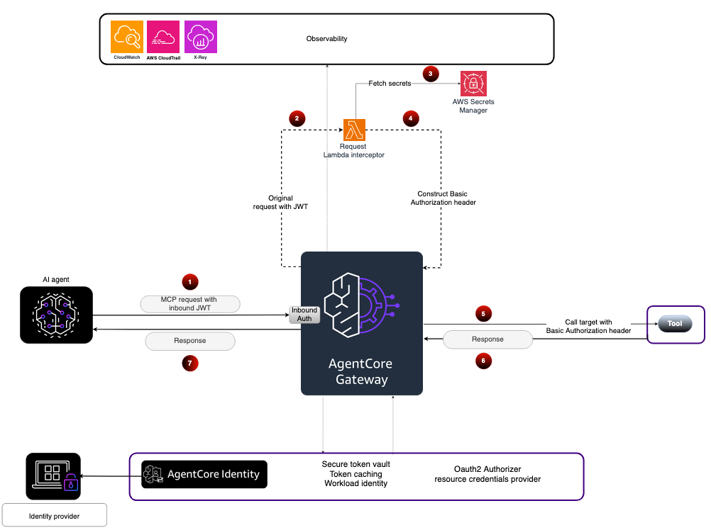
Figure 1: Solution workflow
Note: The system credential stored in Secrets Manager corresponds to a service account in Active Directory (AD). The credential lifecycle requires a one-time manual seed: a system administrator creates the service account in AD and stores the same initial credential in Secrets Manager (necessary because Secrets Manager can’t read a password back from AD). As a security best practice, trigger an immediate rotation after seeding to retire the human-known password using the built-in capabilities of Secrets Manager. From that point forward, Secrets Manager automates the rotation process, periodically generates a new password, and updates both Secrets Manager and AD simultaneously. This eliminates manual credential management in either system. At runtime, the request Lambda interceptor retrieves the current credential from Secrets Manager and presents it to the downstream tool, which validates it against AD. For implementation details on keeping both stores synchronized, see Rotate Active Directory credentials stored in AWS Secrets Manager.
The following steps walk through configuring the request Lambda interceptor and implementing the core of the authentication transformation logic. You can find the complete sample code at Implementing custom authentication for tools integration using Request Lambda Interceptor.
Configure the AgentCore gateway to invoke a request Lambda interceptor for authentication transformation before forwarding the request to the downstream tool.
Important: You must enable
passRequestHeadersconfiguration. Without it, the request Lambda interceptor can’t receive the request header containing the inbound JWT, and the authentication pattern described in this post will not work.
The following example shows the gateway configuration:
The interceptor independently validates the JWT signature as a defense-in-depth measure, protecting against scenarios where the request Lambda interceptor could be invoked through a path that bypasses gateway validation. It fetches the identity provider’s JSON Web Key Set (JWKS) (cached across warm Lambda invocations to avoid repeated network calls), verifies the token’s signature, expiration, and issuer, then returns the decoded claims.
The following code demonstrates JWT validation:
The interceptor retrieves the system service account credential from Secrets Manager. This credential authenticates the AI agent to the downstream tool. The secret is encrypted with a customer-managed AWS Key Management Service (AWS KMS) key and cached in memory for the configured time-to-live (TTL) to minimize API calls while ensuring rotated credentials are picked up promptly.
The following code retrieves the credential from Secrets Manager:
IAM permissions: The interceptor’s execution role requires secretsmanager:GetSecretValue scoped to the specific secret Amazon Resource Name (ARN), and kms:Decrypt scoped to the KMS key used to encrypt it. Follow the principle of least privilege by restricting the resource ARN rather than using wildcards.
Note: The agent doesn’t have access to Secrets Manager. Only the request Lambda interceptor—a deterministic function not influenced by model behavior—retrieves credentials. This isolation is designed to mitigate the risk of adversarial prompts instructing the model to access or exfiltrate authentication credentials, even if the agent is compromised.
The request Lambda interceptor constructs the Basic Auth header using the system credential retrieved for the downstream tool.
The following code shows the core transformation logic.
A request Lambda interceptor in Amazon Bedrock AgentCore Gateway can bridge the gap between the authentication patterns supported by the gateway and the authentication requirements of legacy tool APIs that haven’t yet migrated to modern authentication standards. As demonstrated in this post, the interceptor validates the inbound JWT, retrieves system credentials from Secrets Manager, and constructs the downstream tool’s Basic Auth header without modifying tool schemas or agent implementation.
This approach is an interim integration pattern, not a target architecture. It introduces a credential that must be synchronized between Secrets Manager and the tool’s identity store (such as Active Directory), adding operational overhead for rotation, drift detection, and lifecycle management. The recommended path is to modernize the downstream tool to accept OAuth 2.0, SAML, or OpenID Connect, eliminating stored credentials entirely. Until that modernization is complete, the interceptor isolates credential handling from the agent runtime, designed to help ensure that the agent—a non-deterministic system influenced by user prompts—does not have access to authentication secrets.
If you have feedback about this post, submit comments in the Comments section below.
Post Syndicated from Kaushik Krishnan original https://aws.amazon.com/blogs/big-data/querying-raw-log-data-using-sql-and-ppl-with-the-optimized-engine-in-amazon-opensearch-service/
In this post, you learn how to run fast analytical queries directly against raw log and trace data in Amazon OpenSearch Service using PPL and SQL.
Amazon OpenSearch Service is a fully managed service that helps you deploy, scale, and operate OpenSearch, the open source suite for search, analytics, and observability in the AWS Cloud. OpenSearch Service powers search and real-time analytics workloads, from lexical and hybrid search to log analytics and observability. This post focuses on log analytics, and on a practical question: how much analytical work can you do directly against raw log and trace data, without moving it or reshaping it first?
The new optimized engine in OpenSearch Service answers that question: you can point Piped Processing Language (PPL) and Structured Query Language (SQL) queries at raw log and trace data. The engine returns aggregations, filters, and scans over billions of events on the data exactly as you ingested it. In this post, you follow a single incident investigation, one query at a time. You see how the engine answers each new question, from multi-dimensional breakdowns and latency distributions to error rates and fleet sizing. No precomputed structure sits behind the results.
The optimized engine stores data in the columnar Apache Parquet format and runs queries through Apache DataFusion, a vectorized execution engine, with Apache Calcite planning each query. Because the engine stores data in columns, an analytical query reads only the columns it touches and processes their values in batches, instead of reading each matching document in full. Alongside the columnar format, the engine also keeps an inverted index on the same data, so the query planner routes each operation to the path that serves it best: the columnar engine for aggregations and analytical scans, and the inverted index for selective search and filtering.
You ingest your logs and traces through the same Bulk API and clients you use today, and you write PPL or SQL against them as they land.
The following walkthrough traces a common observability use case, root-cause analysis during a live incident, from the perspective of a site reliability engineer (SRE). The engineer notices elevated latency and a handful of error alerts, with nothing that points to a clear cause. No existing dashboard covers this particular shape of problem, so the engineer opens Amazon OpenSearch Service and starts asking questions of the raw trace data, letting each answer decide the next one. PPL suits this work well. Each command transforms the data and passes it to the next, so the engineer reads a query left to right the same way they think through the investigation.
The walkthrough uses generated OpenTelemetry (OTEL) data from a synthetic load generator, at billion-document scale. The focus is the query capability, that is, what the engineer can express and retrieve directly from raw spans, rather than the specific values in each result.
The first question in any investigation is how widespread the signal is. The engineer breaks errors down across service, HTTP method, and cloud Region in a single pass over roughly 1.1 billion spans.
In plain terms, this query answers the engineer’s first question: where are the failures happening? It counts the error spans and breaks them down by service, HTTP method, and AWS Region in a single pass. Rather than guessing which service to open first, the engineer gets a ranked list of the hardest-hit combinations to investigate.
| errors | total_count | avg_ns | serviceName | http_method | cloud_region |
| 730 | 112,436 | 41,246,806 | export-service | GET | us-west-2 |
| 722 | 111,215 | 41,000,227 | catalog-service | PUT | eu-central-1 |
| 704 | 112,051 | 41,295,539 | image-service | PATCH | us-west-2 |
| 612 | 93,214 | 41,451,145 | healthcheck-service | PUT | us-east-1 |
| 609 | 94,314 | 41,418,897 | auth-service | POST | us-east-1 |
| 609 | 94,414 | 41,447,444 | email-service | PATCH | ap-northeast-1 |
| 593 | 89,726 | 41,047,114 | payment-service | PUT | eu-central-1 |
| 581 | 89,854 | 41,195,643 | file-service | PUT | ap-northeast-1 |
The errors spread across services, methods, and Regions, which points to a systemic pattern rather than a single misbehaving service.
The spread could still reflect one saturated node or a fleet-wide condition. To tell the two apart, the engineer groups failures by exception type, service, and host across the entire index, with no time filter to narrow the scan.
| total_count | exception_type | serviceName | host_name |
| 6 | DeadlockDetectedException | notification-service | ip-10-0-16-34 |
| 6 | IllegalStateException | api-gateway | ip-10-0-180-234 |
| 6 | FileNotFoundException | cart-service | ip-10-0-90-162 |
| 6 | ConnectionRefusedException | feature-flag-service | ip-10-0-8-123 |
| 5 | TimeoutException | auth-service | ip-10-0-97-78 |
| 5 | ConcurrentModificationException | order-service | ip-10-0-165-15 |
| 5 | TimeoutException | coupon-service | ip-10-0-158-25 |
In this sample the counts are low and every row lands on a different host, so no single node stands out. This points to a fleet-wide pattern rather than one bad machine. On production data the same query makes the distinction directly: a code-level bug shows up across many hosts, whereas a single failing node concentrates its errors on one host_name.
Next, the engineer pulls a latency profile for each service. This includes count, average, minimum, and maximum duration, to see how each one behaves and how wide the spread runs.
| serviceName | total_count | avg (ns) | min (ns) | max (ns) |
| event-bus | 11,087,263 | 41,249,552 | 26,113 | 9,304,132,159 |
| scheduler-service | 9,175,964 | 41,251,927 | 21,919 | 13,432,040,933 |
| cdn-service | 9,173,572 | 41,225,385 | 23,468 | 13,768,293,306 |
| ml-inference | 9,036,753 | 41,289,101 | 40,410 | 14,625,084,517 |
| compliance-service | 8,274,635 | 41,294,694 | 41,915 | 7,462,983,016 |
| metrics-collector | 7,804,234 | 41,334,728 | 16,535 | 23,228,217,669 |
| notification-service | 7,688,714 | 41,204,635 | 51,562 | 8,695,311,374 |
| image-service | 7,674,406 | 41,248,069 | 47,473 | 15,350,500,299 |
This gives the engineer a latency fingerprint for each service: the averages sit near 41 milliseconds. But the multi-second maxima reveal a long tail consistent with requests queuing behind a slow dependency.
To track a service-level objective, the engineer computes the error rate (errors against total requests) per service. The query uses an inline conditional, followed by a grouped sum and count, and a final division to produce the error rate.
| errors | total_count | error_pct | serviceName |
| 699,358 | 22,415,308 | 3.12 | payment-service |
| 647,811 | 26,880,140 | 2.41 | checkout-service |
| 562,811 | 30,096,860 | 1.87 | auth-service |
| 316,192 | 24,510,990 | 1.29 | cart-service |
| 288,314 | 30,671,704 | 0.94 | order-service |
| 202,612 | 28,140,552 | 0.72 | search-service |
| 186,012 | 33,820,415 | 0.55 | catalog-service |
| 134,722 | 35,453,247 | 0.38 | image-service |
The engineer defines the error-rate metric in the query itself, and the engine computes it across the full index. The busiest paths, payment and checkout, run near 3 percent, whereas some services stay below 1 percent.
Finally, the engineer sizes how much of the fleet each service spans, a capacity and impact question, and switches from PPL to SQL to express it.
| serviceName | total_count | hosts |
| ml-inference | 35,481,688 | 2,535 |
| image-service | 35,453,247 | 2,491 |
| email-service | 35,443,569 | 2,517 |
| shipping-service | 30,700,372 | 2,438 |
| translation-service | 30,490,570 | 2,502 |
| auth-service | 30,096,860 | 2,466 |
| chat-service | 25,564,111 | 2,449 |
| recommendation-service | 25,366,844 | 2,483 |
The query runs a COUNT(DISTINCT) over a high-cardinality field at billion-row scale, and switching languages mid-investigation costs the engineer nothing more than writing SQL instead of PPL. The host counts cluster in the approximately 2,400–2,540 range, so each service runs across a broad slice of the fleet. That confirms the earlier finding: the errors reflect a fleet-wide pattern, not a single node.
The engineer asked five questions and ran five queries, and each answer shaped the next. The optimized engine served every query directly from raw trace data, across both PPL and SQL, without a rollup table or precomputed summary behind any result.
You don’t need a separate tool to run the queries in this walkthrough.
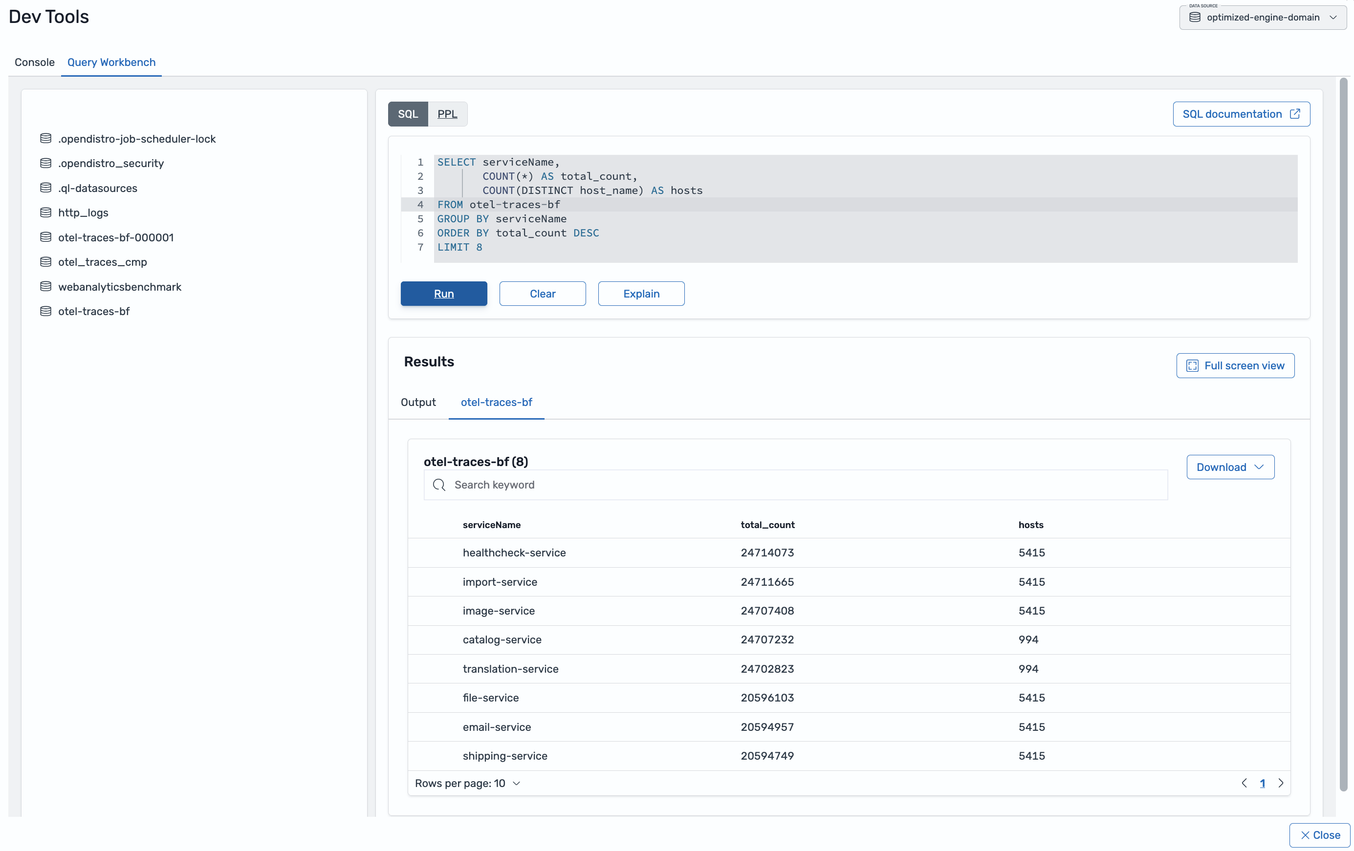
Figure 1: Investigation queries and results grid in Query Workbench
Query Workbench in OpenSearch Dashboards UI gives you a dedicated editor for PPL and SQL. You write a query, run it, and read the results in a grid, using the same queries shown throughout this post. When you want to move from a written query to interactive exploration, Discover runs the same PPL and SQL against your indexes. In Discover, you can filter, expand fields, and drill into individual documents without leaving the page. The same query language works in both places, so you can start an investigation in Discover and carry it into Query Workbench, or the reverse, without rewriting anything.
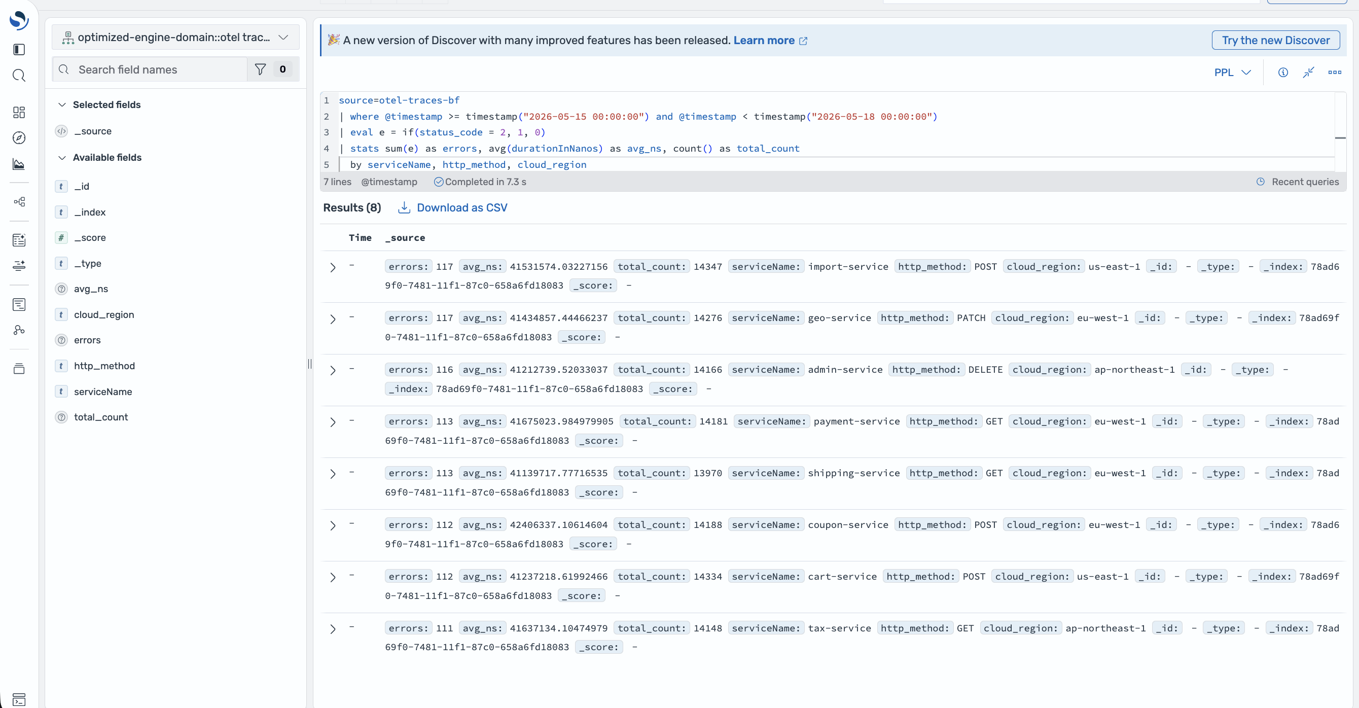
Figure 2: PPL query and field list in Discover
Querying raw data directly only helps if you can afford to keep the raw data. The optimized engine compresses observability data up to 70 percent more efficiently than the default General Purpose engine. That compression turns “keep everything and query it directly” into a practical default. You retain full-fidelity data for the questions you cannot predict in advance. You also pay less to store it than you would to store the raw JSON.
To try the optimized engine, create an Amazon OpenSearch Service domain running OpenSearch 3.5 or later. Then select the Observability use case during setup, which provisions the domain with the optimized engine.
To learn more about configuring and using the optimized engine, see Optimized for Log Analytics in the Amazon OpenSearch Service documentation. For an overview of the service, visit Amazon OpenSearch Service Log Analytics.
For more information, see the blog post Run log analytics for a fraction of the cost with the new engine for Amazon OpenSearch Service.
Give it a try and send feedback to AWS re:Post for Amazon OpenSearch Service or through your usual AWS Support contacts.
Post Syndicated from LastWeekTonight original https://www.youtube.com/shorts/3fCogmuPgeo
Post Syndicated from Michael Fuller original https://aws.amazon.com/blogs/security/security-hub-extended-adds-supply-chain-security-as-its-tenth-category/
Since February, we’ve grown AWS Security Hub Extended from 14 curated partners across 9 categories to 23 partners across 10. At Black Hat this month, 14 of those partners were at the Amazon Web Services (AWS) booth demoing live. Four of those partners delivered theater talks and ten were featured on SecurityLive streaming. We hosted a partner reception that brought our leadership together with partner executives to plan what comes next. These are companies investing real engineering and real go-to-market (GTM) alongside us, and increasingly with each other, because the model resonates with the customers they’re talking to every day. The most common question we heard at the booth was when Supply Chain Security was coming.
It’s here. And that’s the thing I want to spend the most time on today, because it’s the category customers keep asking us about.
Software supply chain risk has moved from a security-team concern to a board-level conversation. SolarWinds showed what happens when a build system is compromised. Log4j showed what a single transitive dependency vulnerability can do at global scale. The xz utils backdoor showed the patience of a maintainer-compromise attack executed over years. Each demonstrated a different dimension of the same problem, and the pace is accelerating. Attackers know that a fast way into an enterprise is through the open source packages that enterprise unknowingly trust.
Every customer I talked to at Black Hat had this on their risk register. Most still hadn’t operationalized a solution, because doing so meant a standalone deployment, a new contract, a new console, and integration work their security team couldn’t prioritize. That’s the friction we aim to remove.
Security Hub Extended now offers Supply Chain Security with Chainguard and Socket as the curated partners. Supply Chain Security uses the same model as everything else in Extended. Every offering has pay-as-you-go pricing, one bill, no required long-term commitment. For enterprises that prefer to continue using the procurement process they always have, Security Hub Extended Private Offers are also available. These are committed term agreements with deeper discounts, the ability to aggregate spend across partners on a single AWS bill, and both monthly and annual payment options throughout the term. You pick the path that fits how you buy.
Chainguard gives you open source dependencies rebuilt from source in a hardened, verified build process, so what enters your environment is malware-resistant and provenance-backed. Their research shows that rebuilding from source would have stopped 98% of known malicious packages from ever reaching production. If you can’t verify the source, it never appears in the Chainguard repository. That’s the filter between the public registry and your developers.
Socket analyzes the actual behavior of open source packages to block malicious dependencies at the time of install. Not after a Common Vulnerability and Exposures (CVE) is published days or weeks later. At the moment the package tries to land in your environment, Socket flags it based on what it does, not what a database says about it. Its reachability analysis then tells you which vulnerabilities are exploitable from your code instead of drowning your team in noise. You pay for the distinct packages you check, not for how often your builds run.
Together, Chainguard and Socket cover the two questions that matter:
Chainguard helps secure the foundation your code is built on. Socket secures the packages you pull into it. Both help protect your software supply chain regardless of where you deploy—across clouds or on-premises. Activate both through Security Hub Extended and their findings flow into Security Hub in OCSF (Open Cybersecurity Schema Framework) alongside everything else, so a supply chain risk is correlated and prioritized next to your endpoint, identity, and cloud signals. From there, it routes out to the downstream tools you’ve already integrated, so it fits the pipeline your builders run today.
Every partner in Security Hub Extended is here because customers told us they needed that capability and that specific solution was already working for them. We add categories because the threat landscape evolves, and we add partners because customers point us to who’s solving those problems well. The goal is straightforward: Simplify adopting the security solutions your peers are already succeeding with, through the AWS relationship you already have.
The full set today spans endpoint, identity, email, network, data, browser, cloud, AI, security operations, and now supply chain. The 23 curated partners are 7AI, Britive, Chainguard, CrowdStrike, Cyera, Island, LayerX, Native Security, Noma, Okta, Oligo, Opti, Palo Alto Networks, Proofpoint, SailPoint, SentinelOne, Socket, Splunk, Sublime, Upwind, Varonis, Zenity, and Zscaler.
Our focus now is deepening integrations and reducing activation friction so these solutions work together, not in isolation. That’s where the real value compounds.
Everything I’ve described so far is the commercial model working: Customers buying best-of-breed security through one AWS relationship with the flexibility they expect. But the bigger vision is the integration layer that makes these tools genuinely better together, not just easier to buy together.
The integration we’re most focused on is cross-partner correlation, turning signals from an endpoint solution, an identity solution, and a cloud solution into one exposure and one attack path instead of three disconnected alerts. Right alongside that, we’re dramatically reducing the activation, deployment, and integration friction so customers go from subscribing to seeing value in hours rather than weeks. Both efforts enable the curated solutions you already trust to deliver stronger outcomes together than they do apart.
That’s the build we’re accelerating with our partners now, and you’ll hear more leading into re:Invent.
If you’re running open source in production and don’t yet have supply chain visibility, start there. Activate Chainguard and Socket through the Security Hub console today. If you’re managing multiple security vendor relationships and want to understand what consolidation looks like with Security Hub Extended, talk to your AWS account team. Pricing for every partner is published on our pricing page, no sales call required. And if you’re already using Security Hub for posture management and threat detection, the Extended plan is available in the same console you already use.
We’re just getting started.
If you have feedback about this post, submit comments in the Comments section below.
Post Syndicated from Harish Ramesh original https://aws.amazon.com/blogs/big-data/fresher-insights-faster-decisions-talabats-near-real-time-analytics-across-aws-and-google-cloud/
talabat is the leading everyday app in the Middle East and North Africa (MENA) region, offering customers a convenient and personalized way to order food, groceries, and other everyday essentials from a wide selection of restaurants and retailers. Founded in Kuwait in 2004, talabat has expanded its operations to the United Arab Emirates, Oman, Qatar, Bahrain, Jordan, Iraq, and Egypt, serving over seven million monthly active customers as of December 2025. talabat is headquartered in Dubai, United Arab Emirates, and in December 2024 successfully completed its initial public offering on the Dubai Financial Market (DFM). As a subsidiary of Delivery Hero SE, talabat uses global expertise to continuously enhance its service, expand its landscape, and drive innovation. With a strong network of partners and riders, talabat connects customers to what they need, when they need it – powering everyday convenience across the region.
In this post, we show how talabat built a hybrid, multi-cloud lakehouse that keeps a single Apache Iceberg copy of streaming data on AWS while enabling governed, near-real-time analytics from Google Cloud Platform (GCP).
Data is the nervous system of talabat’s business. From the moment a customer hits “order” to the second their doorbell rings, talabat’s systems make split-second, data-driven decisions, instantaneously optimizing pricing, dispatch, routing, and order security. Over the years, talabat’s application grew into a landscape spanning two public clouds. Our transactional and operational backbone matured on AWS, where the engineering teams build and operate services. In parallel, a large population of analysts, data scientists, and analytics-engineering pipelines standardized on the Google Cloud Platform warehouse, Google BigQuery.
Both investments are deep, and both deliver value. So the strategic question wasn’t “which cloud do we consolidate on,” but rather “how do we make our data flow cleanly across the boundary between them.” That framing shaped everything that follows. The challenge isn’t only cross-cloud but cross-Region as well, with AWS services hosted in the EU region and the data in the GCP US region.
The following diagram shows how talabat’s data flows between the operational plane on AWS and the analytics plane on GCP.
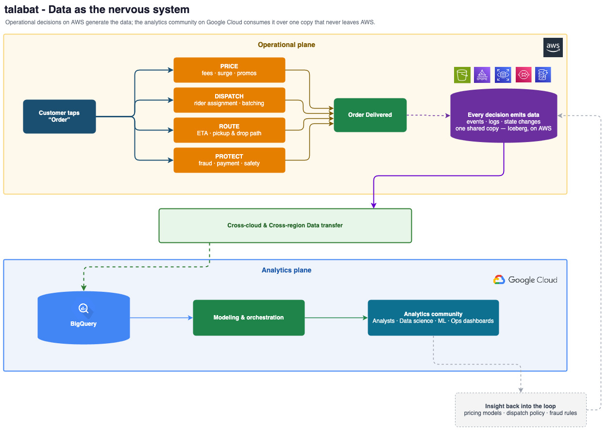
Figure 1: Data flow between the operational plane on AWS and the analytics plane on Google Cloud
Historically, the data engineering team orchestrated the data movement between the two clouds, mandating a physical movement from AWS to GCP, EU to US. Moving this using conventional extract, transform, and load (ETL) tools and frameworks delayed and duplicated the data through multiple hops: Amazon Relational Database Service (Amazon RDS) to Amazon Simple Storage Service (Amazon S3) EU AWS Region, Amazon S3 EU to Amazon S3 US Region, and finally Amazon S3 US to BigQuery US.
Each hop was a copy, and every copy compounded risk: multiple failure points, compounding latency, redundant compute and storage, type fidelity, and most importantly, cross-Region and cross-cloud egress cost.
In short, the old design paid in dollars, latency, and reliability to solve a problem it had created for itself: it moved data so that BigQuery could read it. A classic data warehouse bottleneck. Could we use an open data lake instead? Yes. But the analytics usage is heavy on BigQuery, which limits access through an open source data lake layer. So the redesign started from the opposite premise: keep one copy on AWS and let BigQuery read it in place. That is what the rest of this post describes: a lakehouse for talabat.
Operational systems emit a continuous stream of business events like order lifecycle changes, vendor, menu, logistics and rider signals, and payments information published to Apache Kafka on Amazon Managed Streaming for Apache Kafka (Amazon MSK). These events are encoded as Protocol Buffers and governed by backward-compatible schemas registered in Confluent Schema Registry, so producers and consumers can evolve safely over time.
The requirement on the analytics side is straightforward to state and hard to meet: make these events queryable, correctly typed, within minutes of being produced, and make them queryable from the tools each team already uses.
It’s tempting to view a two-cloud footprint as technical debt. For a real-time business like talabat, it’s simply the terrain, and each side plays to a genuine strength:
Consolidating either side would mean a multi-year migration and a significant regression in capability for one group of users, all to remove a seam between ingestion and analytics. Data engineers decided to engineer the seam instead. The design goal became a single sentence: keep one physical copy of the data on AWS, and read it natively from both clouds. A hybrid data lakehouse makes the “which cloud” question an access-path detail rather than an architectural fork.
Our first attempt inverted the flow we eventually shipped. Raw (also called Bronze) layer data was written from AWS directly into BigQuery-managed Iceberg tables on Google Cloud Storage. On paper, this placed the data closest to the largest consumer base. In practice, writing across clouds on an always-on streaming path introduced a class of problems we did not want to live with:
The lesson was clear: Shift left. The write path should be short, local, and straightforward. The cross-cloud concern belongs on the read path, where it can be made read-only, cached, and retried without affecting the ingestion. That reframing led directly to the architecture we run today.
With the flow inverted (raw data on AWS, read from Google Cloud), we evaluated three ways for BigQuery to read tables that physically live on AWS. We assessed each against four criteria:
| Approach | Assessment |
| Cross-cloud write to Google Cloud Storage | Continue writing bronze into BigQuery-managed Iceberg on Google Cloud Storage. We rejected this for the preceding reasons: it puts a cross-cloud dependency and cross-Region latency on the ingestion hot path. |
| BigQuery Omni | Query AWS resident data through the managed cross-cloud compute of BigQuery Omni. This introduced more managed surface and more constraints than we needed for a read-only bronze layer, and we wanted to own the catalog and trust model directly. |
| Lakehouse federated Apache Iceberg REST catalog (authenticated by IAM) | Let BigQuery read data in Amazon S3 Tables, a capability of Amazon S3 that provides managed Apache Iceberg tables, through a federated catalog that synchronizes AWS Glue Data Catalog metadata, with access authenticated by cross-cloud IAM trust. This met all four criteria, and we chose it. |
The deciding properties were that the raw data doesn’t leave AWS, the format is open Apache Iceberg (so Amazon Athena, Spark, and Iceberg-compatible engines read the same tables), and the cross-cloud relationship is expressed as identity and trust rather than as a recurring copy job.
With the architecture settled on a single Iceberg copy living on AWS, we needed a storage layer purpose-built for Iceberg at scale. Amazon S3 Tables met the requirements without adding operational surface. Table maintenance (compaction, snapshot expiration, and unreferenced file removal) runs automatically as a service-managed policy, avoiding the need for external orchestration jobs that would otherwise grow linearly with table count. Equally important, every table is an Amazon Resource Name (ARN)-addressable resource. That means IAM policies can grant or deny access for individual tables, the same least-privilege model we apply to any other AWS resource, and AWS CloudTrail records every access decision. For a cross-cloud design where the trust boundary is expressed entirely through IAM, having tables that are first-class IAM resources isn’t a convenience but a prerequisite. S3 Tables gave us managed Iceberg housekeeping and fine-grained, auditable access control in a single construct, so the engineering team could focus on the streaming logic rather than the storage plumbing beneath it.
The system has two halves that meet at an open table format:
The single source of truth is Apache Iceberg data in Amazon S3 Tables. Every consumer reads that one physical copy.
The following diagram shows the end-to-end architecture, from event ingestion through storage to consumption paths.
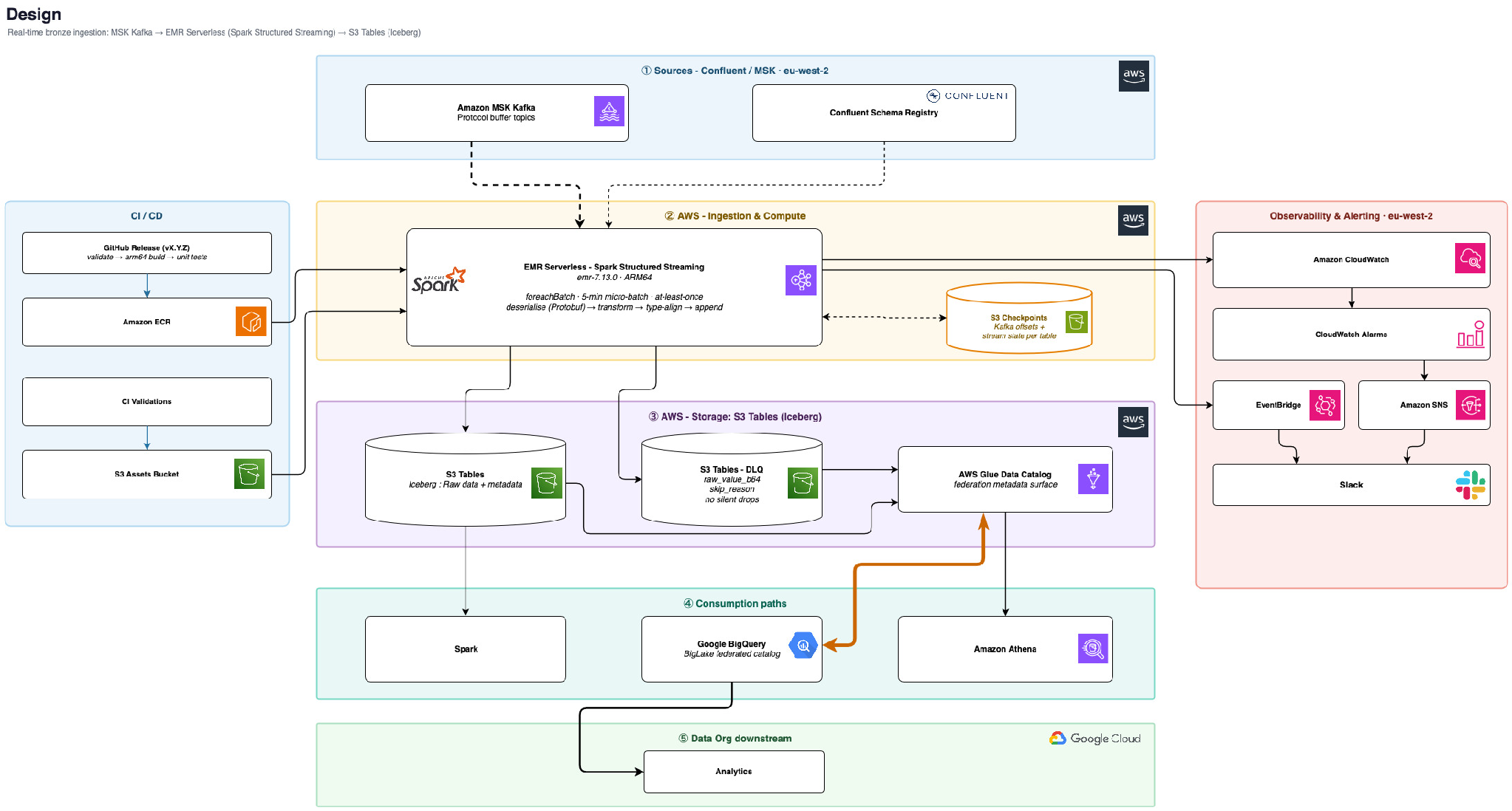
Figure 2: End-to-end architecture from event ingestion through storage to consumption paths
We run one Amazon EMR Serverless Spark Structured Streaming job per Kafka topic (with a prebaked Docker image, emr-7.13.0 on ARM64/Graviton) in the same AWS Region (eu-west-2) as Amazon MSK. Co-locating compute with the event backbone minimizes the data transferred per micro-batch, saving cost and latency. Each job runs the Spark foreachBatch operation with a trigger interval of roughly one to five minutes and at-least-once delivery. Every micro-batch performs five steps:
The cycle repeats without interruption.
This path touches only AWS. There is no cross-cloud dependency, only one deliberate cross-Region hop: compute in the Europe (London) Region (eu-west-2), storage in the US East (N. Virginia) Region (us-east-1). This incurs standard AWS inter-Region data transfer cost, a deliberate choice so that the cross-cloud read from BigQuery stays within the same Region.
Bad records don’t block the stream. They land in a dedicated dead-letter queue (DLQ) table (<table>_dlq) in a separate S3 Tables bucket, storing the raw payload (raw_value_b64) and a skip_reason. Nothing is silently dropped. The DLQ tables are registered with the AWS Glue Data Catalog through Lakehouse, so engineers can inspect failures from Amazon Athena or BigQuery.
From this point on, Amazon S3 Tables is the source of truth.
This is the heart of the design. BigQuery reads the S3 Tables Iceberg data through a Lakehouse federated Apache Iceberg REST catalog, a read-only catalog on the Google Cloud side that points at the AWS resident tables. Three mechanisms make it work.
Amazon S3 Tables exposes an Apache Iceberg REST catalog interface, and Google Lakehouse speaks that same standard. Because both sides agree on the Iceberg on-disk format and REST catalog protocol, no translation layer or data copy is required. BigQuery reads the identical Iceberg data files that Athena and Spark read.
On the Google Cloud side this is a single Lakehouse federated catalog. A table surfaces to analysts as
talabat-data.s3tables-glue.catalog.orders.
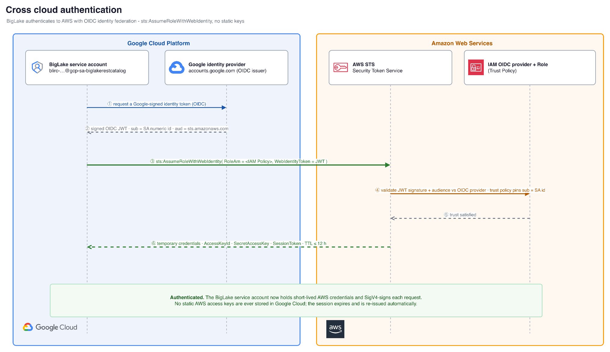
The Lakehouse catalog authenticates to AWS as a Google-managed service identity (the Lakehouse REST-catalog service account) that an AWS Identity and Access Management (IAM) role trusts through OpenID Connect (OIDC) federation with
accounts.google.com, usingsts:AssumeRoleWithWebIdentitywith the service account’s numeric ID pinned in the role’s trust policy. Requests to the S3 Tables Iceberg endpoint are SigV4-signed. It’s the same AWS request-signing scheme that any AWS SDK uses, scoped to the S3 Tables service. In other words, the handshake isn’t a proprietary connector. It’s standard AWS request signing performed by a trusted external identity.The trust is codified as infrastructure as code (IaC) on the AWS side: granted least-privilege, and revocable at any time. The following diagram shows this authentication sequence.

Figure 3: Cross-cloud authentication sequence between the Lakehouse catalog and AWS IAM
For a step-by-step walkthrough of this trust relationship, creating the IAM role, validating the token’s audience and subject, and pinning the Lakehouse service-account identity in the trust policy, see Create and manage AWS Glue federated datasets and Set up cross-cloud Lakehouse for AWS Glue.
The federated catalog periodically synchronizes table metadata from the AWS Glue Data Catalog that fronts S3 Tables. Newly created tables and new data become visible to BigQuery on a short refresh cycle (approximately 300 seconds). Reads are served against the live Iceberg data. Only the catalog pointers are synchronized.
The result is that a table written once on AWS appears in BigQuery as an ordinary catalog object and can be queried with standard SQL, while the bytes don’t leave AWS and the format stays open.
The following section explains the authentication handshake shown in the architecture diagram. The Lakehouse catalog service account presents a Google OIDC JSON Web Token (JWT), which AWS validates through the IAM OIDC provider, returning short-lived credentials scoped to read-only S3 Tables access.
Together these four steps are the whole handshake: a trusted issuer, a role that only our service account can assume, a least-privilege read grant, and a catalog bound to that role.
Operating an open, federated catalog across clouds taught us to treat table metadata as a first-class operational concern. In practice this means:
These are small, well-understood settings once we know how to set them, and they are the difference between a catalog that simply works and one that drifts.
After a source is live, the same Iceberg table is available three ways over one physical dataset.
Nobody waits for a nightly export, and nobody reconciles three divergent copies. There is only one.
The qualitative benefits are already clear:
Looking ahead, we plan to broaden source coverage by onboarding the remaining high-value event streams and batch stores onto a hybrid one-configuration pattern. We’re formalizing end-to-end freshness objectives and the observability around them: batch-level metrics, dead-letter monitoring, and catalog-synchronization health. We will continue tuning snapshot retention and compaction so the cross-cloud catalog stays fast and reliable as the number of tables grows. More broadly, we intend to make “written once, read by any engine” the default for new datasets beyond the bronze layer, leaning further into open table formats as the connective tissue between cloud service providers.
Being on two clouds is often framed as a problem to migrate away from. It’s simply the terrain for talabat. The event backbone is prominent on AWS, and the analytics community operates on BigQuery. By making Amazon S3 Tables with Apache Iceberg the single source of truth on AWS and letting BigQuery consume it read-only through a Lakehouse federated Iceberg REST catalog secured by cross-cloud IAM trust, we turned a two-cloud constraint into a single governed dataset that engines can read within minutes. The write path stays short, local, and reliable. The cross-cloud concern lives on the read path, where it belongs, expressed as open standards and identity, not as data movement.
That is the handshake: one copy of the data on AWS, an open catalog contract, and a signed, trusted, revocable identity reaching across the cloud boundary to read it.
This post focuses on reading AWS resident data from BigQuery. For the broader multi-cloud Lakehouse pattern, including federating catalogs from other systems into the AWS Glue Data Catalog, see Multi-cloud Lakehouse architecture on AWS for agentic AI.
Post Syndicated from Mazrim Mehrtens original https://aws.amazon.com/blogs/big-data/powering-agentic-ai-with-real-time-streaming-data-on-aws/
Two years ago, the conversation about streaming data and generative AI centered on a straightforward question: how do you feed real-time context into a large language model (LLM) so it can answer questions using fresh data? We explored that question in our 2024 blog post, “Exploring real-time streaming for generative AI applications,” which introduced patterns for connecting streaming pipelines to foundation models.
The landscape has shifted. Today’s generative AI systems don’t only answer questions. They observe, reason, and act. Agentic AI applications have moved from research prototype to production reality. Agentic AI-powered data pipelines now monitor streaming telemetry, detect anomalies, decide on remediation strategies, and execute actions without human intervention. They maintain memory across sessions, query live data sources on demand, and coordinate with other agents to solve complex problems.
This shift demands a fundamentally different relationship between streaming infrastructure and AI. It’s no longer enough to inject context into a prompt. You need architectures where streaming data continuously powers autonomous agent action and keeps a real-time lakehouse fresh for training and retrieval. That data also flows into multiple consumption patterns, such as generative business intelligence (BI) for humans, standardized protocols for agent queries, and proactive memory hydration for low-latency agent context.
This post introduces three architectural patterns that together form a unified streaming backbone for the agentic AI era:
The following sections explore each pattern in depth.
You’re watching a live football match. As a striker receives the ball in the box, AI-generated commentary appears on screen: “This is Smith’s third touch in the penalty area in the last 3 minutes. His conversion rate from this zone is 34% this season.” That insight was computed from streaming event data, passed through a feature pipeline, and fed to a generative AI model. All of this happened within the time it takes the striker to turn and shoot.
This pattern combines two capabilities that are often treated separately: using real-time data to continuously improve AI models, and using real-time data to invoke those models for immediate action. The streaming pipeline does both: it builds the features that train the model and the features that drive inference.
Streaming events (user interactions, sensor readings, game events, and transaction records) flow into Amazon Managed Streaming for Apache Kafka (Amazon MSK) or Amazon Kinesis Data Streams. Amazon Managed Service for Apache Flink processes these events through windowed aggregations (tumbling windows, sliding windows, or session windows) to produce features: rolling averages, counts, ratios, behavioral sequences, or other derived signals relevant to your use case.
These features serve two paths simultaneously:
The inference path: At the end of each window (or on each event, depending on your latency requirements), features are passed to a generative AI or machine learning (ML) inference endpoint: Amazon Bedrock for generative output, or Amazon SageMaker for custom models. The model produces a result (commentary, a recommendation, a personalization decision, or a risk score) and the pipeline acts: posting content to a user, updating a recommendation feed, sending a notification, or writing to a downstream system.
The training path: The same streaming features are continuously written to a real-time data warehouse or lakehouse such as Apache Iceberg tables on Amazon S3 Tables, a capability of Amazon Simple Storage Service (Amazon S3), that keeps training datasets fresh. Amazon SageMaker lakehouse architecture provides unified access for training jobs and fine-tuning pipelines. As new data streams in, your models can be retrained or fine-tuned on data that’s minutes old rather than days old. This matters for domains where patterns shift quickly, such as fraud detection, personalization, and industry dynamics.
Amazon S3 Tables handles the Iceberg table management automatically, including compaction, snapshot management, and metadata optimization. Your team focuses on feature logic rather than storage operations. The AWS Glue Data Catalog makes these tables discoverable across training jobs, inference pipelines, and analytics consumers. Glue Data Catalog supports business context and semantic search. This context helps models discover and select the right data asset for any given task.
Real-time sports commentary: Streaming game events (passes, shots, player positions) flow through Apache Flink on Managed Service for Apache Flink, which computes rolling features (possession percentage, shot frequency by zone, player heat maps). These features feed a generative AI model through Amazon Bedrock that produces natural-language commentary and statistical insights in real time. Simultaneously, the features are written to S3 Tables to improve the model’s understanding of game patterns over time.
Streaming personalization: User clickstream data flows through Managed Service for Apache Flink, which computes behavioral features (session duration, category affinity scores, recency-weighted purchase history). These features invoke a personalization model that updates the user’s experience in real time by reranking product recommendations, adjusting content feeds, or triggering targeted offers. The same features feed the lakehouse to retrain the personalization model nightly.
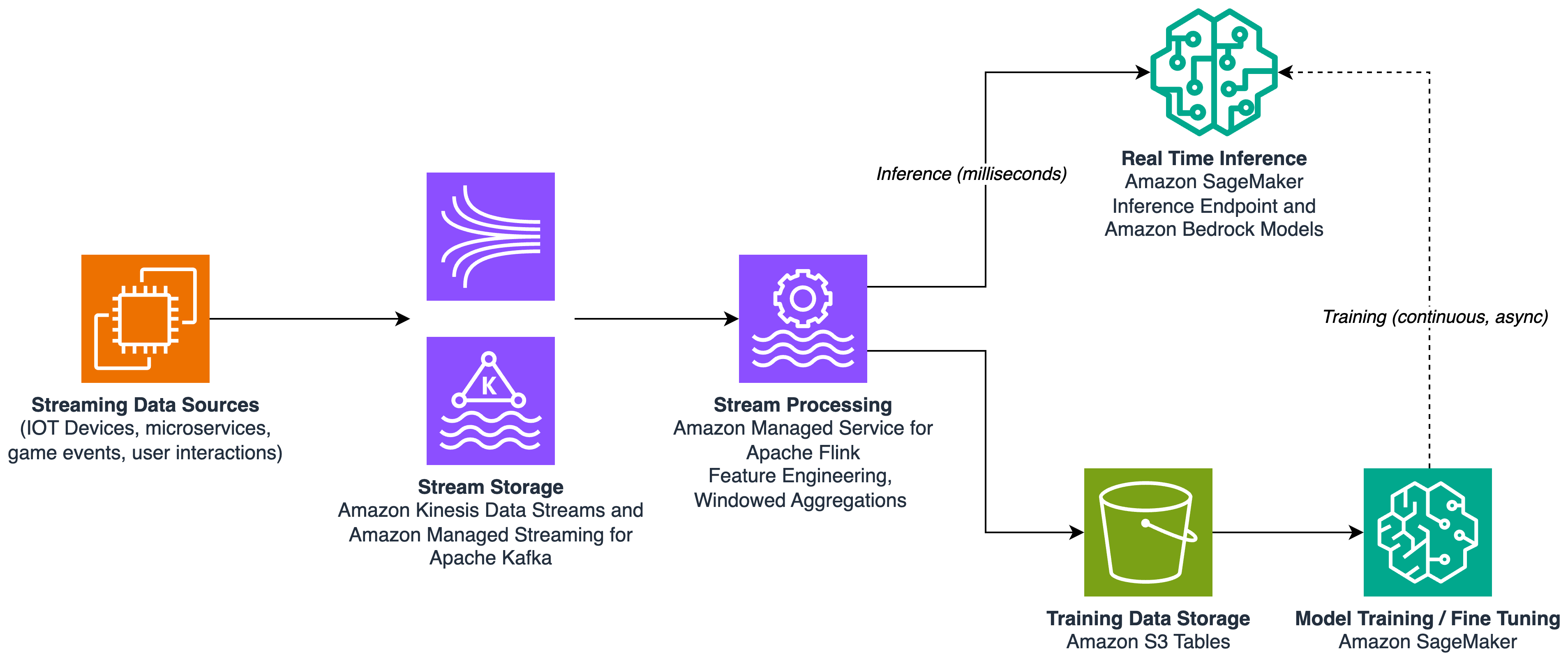
Figure 1: Streaming feature engineering feeding a real-time inference path and a continuous training path
At 2:47 AM, a pressure sensor on a manufacturing line begins drifting. Within seconds, a streaming pipeline detects the anomaly, assembles full context (device history, maintenance schedule, correlated sensor readings), and invokes an agent that opens a maintenance work order, adjusts the device’s sampling rate, and notifies the on-call engineer. All of this happens before a human sees an alert.
Pattern 1 invokes inference on every window or event. It runs continuously. Pattern 2 adds to this approach: the streaming pipeline continuously analyzes data and invokes an agentic workflow when specific conditions are met or a pattern is detected. The pipeline is the sensor. The agent is the responder. Dynamic rules are the bridge between them.
The key distinction is that the events and triggers are dynamic. They’re defined by rules programmed into the streaming pipeline or traditional ML models for prediction or detection. The pipeline determines when and how the agent is triggered, making the system fluid and adaptive. You can update detection logic without redeploying the agent. You can add new anomaly patterns without changing the response logic.
Streaming telemetry flows into Amazon MSK or Amazon Kinesis Data Streams. Managed Service for Apache Flink runs continuous anomaly-detection logic, such as statistical models, windowed aggregations, threshold-based rules, or ML-based scoring. Critically, when Flink detects an anomaly, it doesn’t only publish a raw alert. It assembles a context package: the anomaly details, relevant historical data, correlated signals from other streams, and metadata the agent needs to act immediately.
This context package is published to a downstream topic and consumed by an Amazon Bedrock AgentCore agent. Because the pipeline has already assembled full context, the agent doesn’t waste time gathering information. It can reason and act immediately. AgentCore Runtime hosts the agent, AgentCore Observability provides tracing and logging, and AgentCore Memory maintains state across invocations (so the agent knows, for example, that this is the third anomaly from this device this week).
The benefit of this pattern over a polling-based or scheduled approach is twofold:
The rules that trigger invocation are a powerful abstraction. They can be simple thresholds (“temperature exceeds 95°C”), statistical (“value deviates more than 3σ from the rolling mean”), or ML-based (“anomaly score from an embedded model exceeds 0.85”). You can update these rules dynamically by adding new detection patterns, adjusting sensitivity, or routing different anomaly types to different agents.
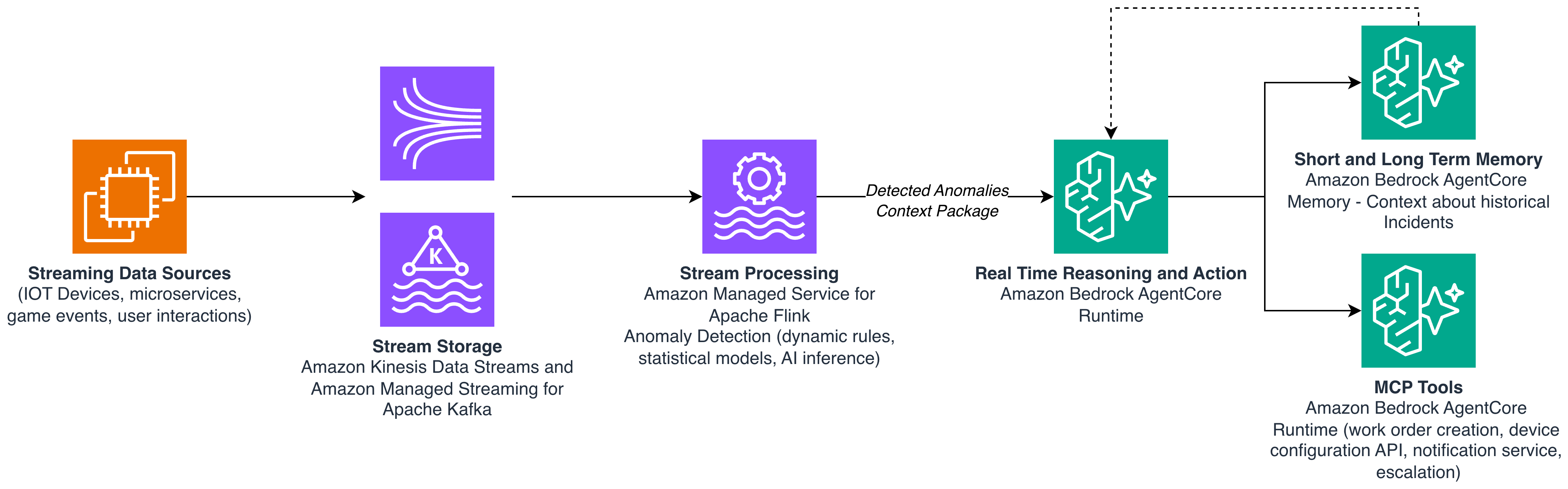
Figure 2: Event-driven agent invocation triggered by anomaly detection in the streaming pipeline
A customer messages their bank: “Was that $847 charge at the airport legitimate?” The agent responds in under two seconds with full context (the customer’s recent travel pattern, the merchant’s fraud-risk score, and the transaction details) because all of this was already loaded into the agent’s context layer through streaming CDC. A reactive agent without this synchronization would need to make five separate API calls across three systems, taking 8–12 seconds and risking timeout failures.
This pattern addresses a fundamental question: how proactive should your agent be about gathering context?
A proactive agent has the full context, continuously synchronized with the state of the world. When a user asks a question, the agent already has the relevant knowledge from context. It responds from memory rather than making expensive external calls. A reactive agent starts cold. It knows nothing until it queries for information, making multiple calls across security boundaries, handling authentication, and stitching together data from disparate sources. For latency-sensitive use cases, where a user sends a prompt and expects a fast response, this difference is critical.
Real-time context synchronization uses CDC and streaming pipelines to keep agent memory current. The agent’s knowledge graph becomes a synchronized replica of the distributed systems it needs to reason about.
No agent is purely proactive or purely reactive. The design decision is: what data should be pre-loaded, and what should be fetched on demand? This is a spectrum, and where you land depends on three factors:
Streaming pipelines (Managed Flink reading from Amazon MSK, Kinesis Data Streams, or CDC streams from operational databases) continuously process events and write aggregated results to the agent’s knowledge graph, or the context layer. These stores can take multiple forms depending on your access patterns:
For data that isn’t pre-loaded, the agent falls back to on-demand retrieval. This applies when the data is too large, changes too rarely to justify streaming, or is needed only in edge cases. The Model Context Protocol (MCP) provides a standardized interface for this. MCP servers expose heterogeneous data sources through a uniform protocol. The agent queries MCP when it needs context that isn’t in its synchronized memory.
This same real-time context synchronization pattern serves different consumers:
AI agents access fresh context through a real-time knowledge graph or a context layer, and MCP servers (pull tier), as in the preceding sections.
Human analysts and executives access the same context layer, which can directly query Apache Iceberg tables on S3 Tables through its direct query mode. Amazon Quick chat provides natural-language access to real-time lakehouse data. No intermediate warehouse is required. This is the generative BI expression of the same underlying pattern: streaming data keeps the lakehouse current, and Amazon Quick gives humans conversational access to it.
Training and fine-tuning pipelines access the synchronized lakehouse through Amazon SageMaker Lakehouse, keeping models fresh (as described in Pattern 1).
The underlying principle is the same across consumers: streaming pipelines synchronize distributed data into accessible stores, and each consumer accesses those stores through the interface that fits their needs.
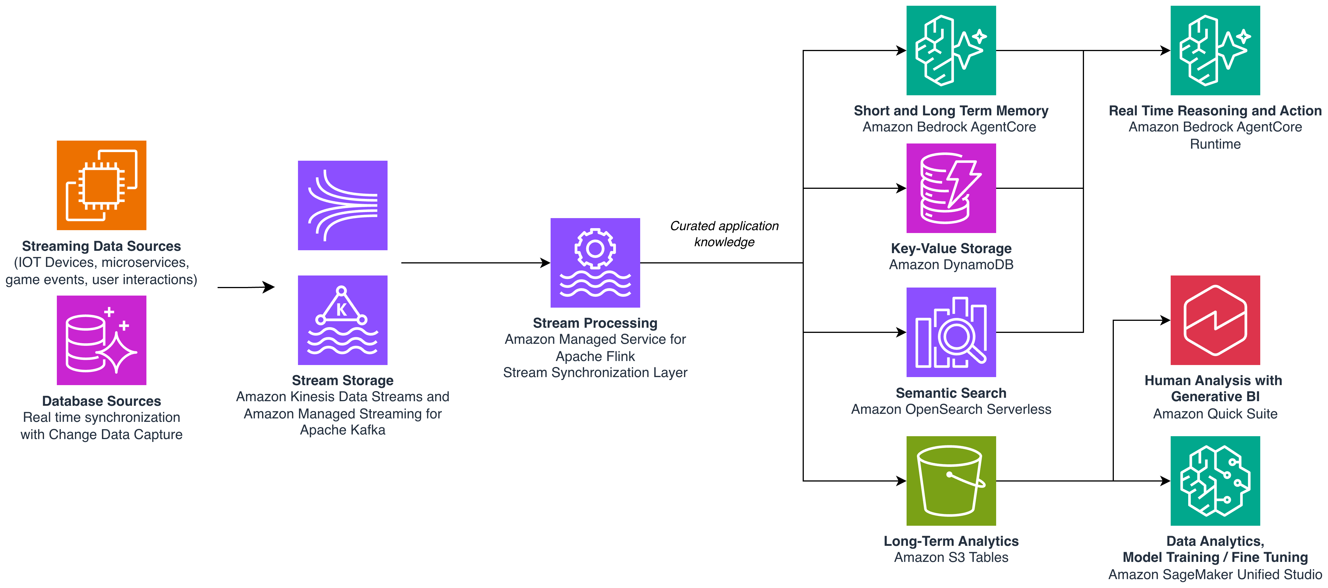
Figure 3: Real-time context synchronization serving agents, analysts, and training pipelines from shared stores
The three patterns in this post form a unified architecture built on a single streaming backbone:
Pattern 1 uses streaming pipelines to build features that simultaneously drive real-time inference and keep training data fresh. Your models improve continuously while serving predictions in real time.
Pattern 2 uses streaming pipelines as intelligent sensors that detect anomalies and invoke agents with full context already assembled. This separates detection logic from response logic for maximum flexibility.
Pattern 3 uses streaming pipelines to synchronize distributed system state into the agent’s context layer, making agents more proactive and serving multiple consumers (agents, humans, and training jobs) from the same pre-loaded data.
The streaming infrastructure you build (Amazon MSK, Amazon Kinesis Data Streams, Amazon Managed Service for Apache Flink, and Amazon S3 Tables) serves all three patterns simultaneously. A Flink application can compute features for inference (Pattern 1), detect anomalies that trigger agents (Pattern 2), and synchronize state into agent memory (Pattern 3).
To get hands on with the patterns described in this post, refer to Agentic AI-Powered anomaly detection: Spotting anomalies in real-time.
You don’t need to implement all three patterns at once. Start with the one that addresses your most pressing need. But design your streaming infrastructure knowing it will serve multiple patterns. In the agentic AI era, every stream is a potential input to an agent, a model, and a human decision-maker.
Post Syndicated from Rommel Sunga original https://aws.amazon.com/blogs/messaging-and-targeting/send-rich-rcs-messages-with-aws-end-user-messaging-rcs/
When a customer asks where their order is, a plain text reply answers the question. But a rich RCS message with a product photo, a tappable confirmation button, and a calendar chip helps the customer act on it. Rich Communication Services (RCS) messages deliver branded, interactive content, including images, rich cards, carousels, and suggestion chips, to the messaging app already built into the customer’s phone. Unlike Short Message Service (SMS), RCS messages come from a verified sender with your brand name and logo, deliver over a data connection, and support read receipts and structured replies. AWS End User Messaging RCS provides the SendRcsMessage API, a managed way to send RCS messages through a single integration point instead of separate integrations for each carrier.
This post is for developers and solutions architects who want to add RCS messaging to their customer engagement workflows on AWS. It shows how to send every RCS content type (text, files, rich cards, carousels, and suggestions). It also shows how to control delivery with message expiration and SMS fallback, using Python and the AWS End User Messaging RCS API.
The post focuses on the SendRcsMessage API, which is specific to RCS and is the only one of the two that supports rich cards, carousels, and suggestions. The SMS API’s SendTextMessage can also deliver over RCS when you pass an RCS agent as the origination identity, but it is limited to plain text. Every example that follows uses SendRcsMessage.
Before you run the examples in this post, you need the following:
VERIFIED.SendRcsMessage support. Run pip install --upgrade boto3 to get the latest version.If you’re new to RCS on AWS, see Getting started with RCS on AWS End User Messaging SMS to create your agent. You pay standard RCS rates for RCS messages, including messages sent to test devices.
The AWS Identity and Access Management (IAM) principal that runs the examples needs permissions for the following actions:
sms-voice:SendRcsMessage, to send RCS message types.sms-voice:SendTextMessage, to send the plain text comparison example and any SMS fallback messages.sms-voice:DescribeRcsAgents, to check that your agent is Active.sms-voice:DescribeVerifiedDestinationNumbers, to confirm a registered test device is VERIFIED, if you send to one.If you use the SMS fallback example, you also need a phone number or sender ID in your account that can send SMS to the destination country. RCS and SMS are separate origination identities: the RCS agent sends the RCS message, and the fallback needs its own SMS-capable identity.
If you send media from Amazon Simple Storage Service (Amazon S3), the bucket needs a resource policy granting the sms-voice.amazonaws.com service principal s3:GetObject, shown in the “File messages” section. If you use server-side encryption with AWS Key Management Service (AWS KMS) keys for your bucket, your KMS key policy must also grant the service access. For two-way messaging, your SNS topic needs a resource policy allowing the service to publish to it. For details, see Two-way messaging in the AWS End User Messaging SMS User Guide.
Create a config.json file in your project directory to store the RCS agent Amazon Resource Name (ARN) that sends the messages and the recipient phone number in E.164 format:
OriginationIdentity accepts the RCS agent ID (RcsAgentId) or ARN (RcsAgentArn), and also a pool ID or pool ARN. The examples use the agent ARN because it stays unambiguous when an account has more than one agent, but the shorter agent ID works the same way.
The config.json file is for local testing only. In production, don’t hardcode phone numbers and identifiers. Use AWS Secrets Manager, AWS Systems Manager Parameter Store, or environment variables instead.
Each example in this post builds a message_content dictionary and sends it with the following code:
For production use, wrap the send call with error handling to manage throttling and validation failures:
The following sections show only the message_content for each message type. To send any of these messages, use the shared sending code from this section. The examples follow one scenario: AnyCompany, a fictitious retailer, messaging a customer about an order.
Text messages are the most basic RCS content type. You can send plain text two ways. The SendTextMessage API, the same API used for SMS, delivers over RCS when you pass your RCS agent ARN as the origination identity:
The SendRcsMessage API sends the same text as a TextMessage content type, and additionally supports suggestion chips, message expiration, and per-message fallback. An RCS text also arrives as a single message regardless of length, while carriers split SMS over 160 characters into segments that can arrive out of order.
FallbackConfiguration, recipients who can’t receive RCS get nothing.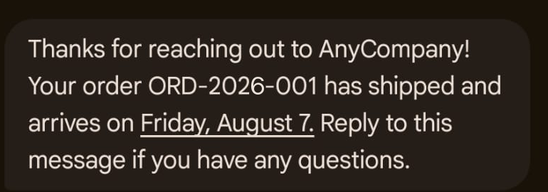
Figure 1: RCS text message confirming that order ORD-2026-001 has shipped
The following is the message_content for the preceding message:
With file messages, you send a single image, video, audio file, or PDF that renders as inline media in the recipient’s messaging app. FileUrl accepts two URL forms, and they fail in different places.
With an S3 URL (s3://amzn-s3-demo-bucket/object-key), the API checks at request time that the object exists, is within the size limit, and is readable with the permissions you granted the service. If any of those checks fail, the call returns a ValidationException describing the problem, so you find out at send time. The service then retrieves the object, rehosts it, and generates a time-limited presigned URL for delivery to the device.
With an HTTPS URL, the URL is passed through to the carrier and isn’t checked the same way at request time. The API accepts the request. Problems such as an unreachable host, a URL that requires authentication, or an unsupported media type surface at delivery instead of in the API response. The URL must be publicly accessible with no authentication. The API doesn’t support plain http:// URLs.
Use S3 URLs when you want bad media to fail loudly at send time. Use HTTPS URLs for media already published on a public CDN, and monitor delivery events for failures.
FileUrl: required, S3 or HTTPS URL, up to 2,000 characters.ThumbnailUrl: optional, JPEG or PNG, recommended for video and PDF.To deliver from Amazon S3, add the following bucket policy so the service can read your objects:
Replace amzn-s3-demo-bucket with your bucket name. To restrict access to a prefix, replace /* in the Resource ARN with a path such as arn:aws:s3:::YOUR-BUCKET/rcs-media/*.

Figure 2: RCS file message rendering an inline PDF attachment
The following is the message_content for the preceding message:
A rich card combines media, a title, a description, and suggested actions into a single structured message. Rich cards work well for product highlights, booking confirmations, appointment details, and promotional offers.
CardContent requires at least one of Media, Title, or DescriptionCardOrientation is required: VERTICAL or HORIZONTAL. Use VERTICAL because horizontal orientation truncates images on iOS.Media Height: SHORT (112 density-independent pixels), MEDIUM (168), or TALL (264). IOS ignores this value.OpenUrl suggestions for links.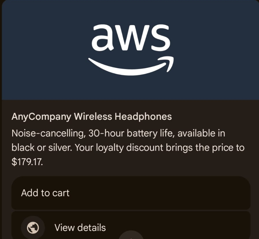
Figure 3: Vertical rich card with a product image, title, description, and action buttons
The following is the message_content for the preceding message:
A carousel displays 2–10 rich cards in a horizontally scrollable strip. Carousels fit browse-and-compare experiences such as product catalogs, service menus, plan comparisons, and location listings. Carousel cards use the same content model as standalone rich cards, with two differences: cards always render in a vertical layout, and the TALL media height is not supported.
CardWidth: SMALL (180 density-independent pixels) or MEDIUM (296). All cards share the same width.Media Height: SHORT or MEDIUM only.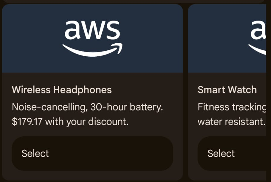
Figure 4: Carousel showing the Wireless Headphones and Smart Watch cards, each with a Select button
Scrolling right reveals the remaining cards:
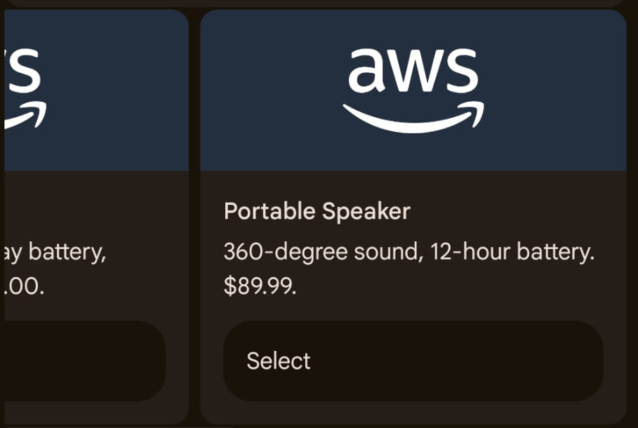
Figure 5: Carousel scrolled to the Portable Speaker card
The following is the message_content for the preceding message:
Suggestions are the interactive chips you saw in the earlier examples. They guide recipients through a conversation with predefined replies and actions, without typing. RCS supports six suggestion types: Reply, OpenUrl, DialPhone, ShowLocation, RequestLocation, and CreateCalendarEvent, and you can mix them in one message on any content type. Message-level suggestions live in a Suggestions array that is a sibling of Content, not nested inside it. Card-level suggestions live inside each card’s CardContent.
Every suggestion requires a Text label and PostbackData. The postback data is invisible to the recipient and comes back to your application when the chip is tapped. Encode routing information there (for example, appt_confirm_12345), and route logic on postback data rather than display text.
Text label: up to 25 characters; PostbackData: up to 2,048 characters, both required on every suggestion.OpenUrl Url must begin with https://. Set Application to WEBVIEW with a WebviewViewMode of FULL, HALF, or TALL to keep the recipient inside the messaging app.DialPhone PhoneNumber must be in E.164 format.CreateCalendarEvent requires Title, StartTime, and EndTime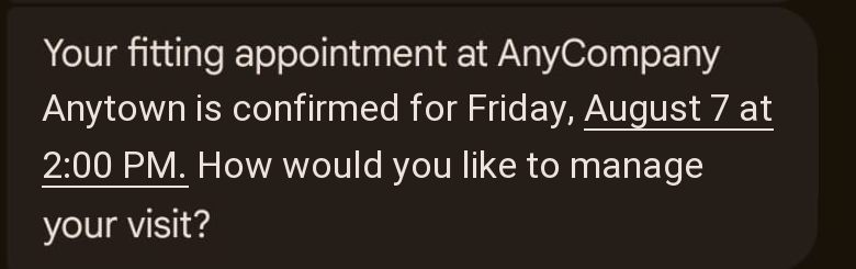
Figure 6: RCS message confirming a fitting appointment at AnyCompany Anytown
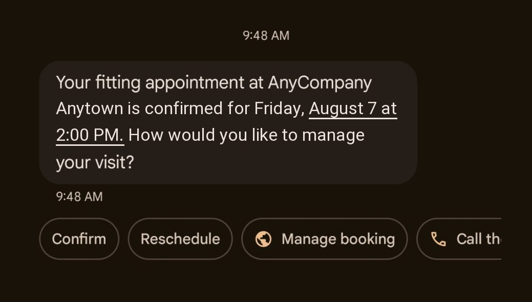
Figure 7: Suggestion chips below the appointment message: Confirm, Reschedule, Manage booking, and Call the store
Scrolling the chip row reveals the remaining suggestions:
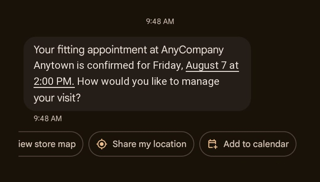
Figure 8: Remaining suggestion chips: View store map, Share my location, and Add to calendar
The following message_content combines all six suggestion types on one text message:
When the recipient taps a chip, the messaging app sends the chip text back into the conversation as a reply:
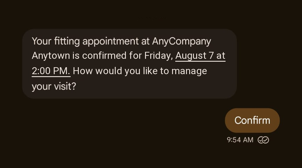
Figure 9: Tapping Confirm sends the chip text back as a reply, shown with a read receipt
The tap arrives as an inbound event on your two-way SNS topic. The messageBody field contains a JSON string with a type of SUGGESTION, the display text, and the postback data:
Note the casing difference: request fields use PascalCase (PostbackData), while inbound events use camelCase (postbackData). A RequestLocation tap delivers the recipient’s coordinates in a separate inbound location event.
The TimeToLive parameter sets an expiration window in seconds on a SendRcsMessage request. If the message is not delivered within that window, the service removes it and the recipient never sees it. This matters for time-sensitive content such as one-time passwords (OTPs): a verification code that arrives after the code has expired only confuses the customer.
TimeToLive: integer seconds, 1–172,800 (48 hours). Use at least 10 seconds so the carrier can attempt delivery.TimeToLive means no expiration window.TTL_EXPIRATION_REVOKED event (message removed, safe to send a fallback) or TTL_EXPIRATION_REVOKE_FAILED (revoke failed, the message might still deliver, so weigh the duplicate risk)
Figure 10: RCS verification code delivered within its five-minute expiration window
The following example sends an OTP that expires after five minutes. TimeToLive is a request parameter, a sibling of RcsMessageContent:
Fallback is optional, and without it a recipient who can’t receive RCS gets nothing. The FallbackConfiguration request parameter routes the message to SMS or Multimedia Messaging Service (MMS). Fallback applies when the device or carrier doesn’t support RCS, when the channel rejects the message, or when the TimeToLive window expires first.
Channel: required, SMS or MMS.MessageBody: required for SMS fallback, up to 1,600 characters (compared with 3,072 for the RCS text body); MMS fallback requires at least one of MessageBody or MediaUrlsOriginationIdentity for the fallback: a phone number or sender ID registered in your account that can send SMS or MMS to the destination country. Pools and RCS agents are not accepted here.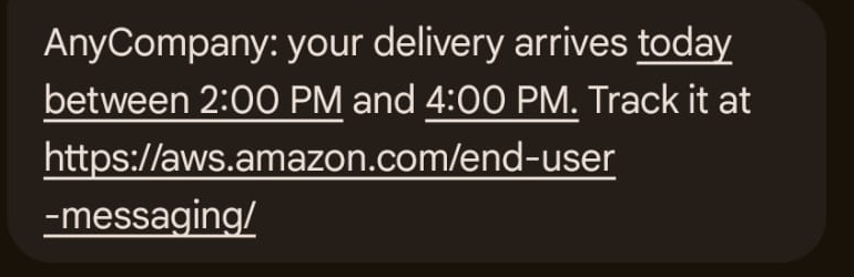
Figure 11: AnyCompany delivery notification delivered over RCS
On a device without RCS, the SMS fallback version arrives instead from the fallback phone number.
The following example sends a delivery notification with an SMS fallback from a dedicated phone number:
To track outcomes, pass ConfigurationSetName on the send call so delivery, read, expiration, and fallback events route to your configuration set’s event destinations. Set up event destinations before you send, because they don’t retroactively capture events.
To avoid incurring future charges, delete the resources that you created during this walkthrough:
In this post, you learned how to send every RCS content type with AWS End User Messaging RCS, including text messages, file messages, rich cards, carousels, and suggestions. You also learned how to control delivery with message expiration and per-message SMS fallback. You sent each type from a short Python script, with one shared sending pattern across all content types.
The SendRcsMessage API keeps one pattern across all content types: a Content object for the message body and a sibling Suggestions array for interactivity. Moving from a plain text notification to a full product carousel is a change to one dictionary.
Next steps:
TimeToLive values with per-message SMS or MMS fallback for each use case.Create your first RCS agent in the AWS End User Messaging SMS & RCS console and send a test message today. Tell us about your experience: share your use cases and questions in the comments.
Post Syndicated from Ali Alemi original https://aws.amazon.com/blogs/big-data/amazon-msk-simplifies-configuring-custom-domain-names/
Previously, you had to manually override the advertised listener on each broker and repeat it every time a broker was added. This approach was operationally heavy and could not be implemented on a cluster in KRaft mode. With Amazon Managed Streaming for Apache Kafka (Amazon MSK), you can now configure custom domain names for your Provisioned clusters using a single property. This works for clusters in both ZooKeeper and KRaft mode. Now you define the domain once and Amazon MSK applies it across every broker, so custom domain names keep working through scaling of the MSK cluster.
Amazon MSK is a fully managed service for building and running applications that use Apache Kafka to process streaming data. By default, Amazon MSK brokers advertise addresses that AWS generates (for example, b-1.cluster-name.kafka.us-east-1.amazonaws.com) to connecting clients. These addresses are unique to each cluster and change when a cluster is recreated.
Many organizations need a static, customer-controlled endpoint that stays the same regardless of the underlying cluster. They achieve this with a custom domain name, so that they can:
Until now, the only way to do this was to override the advertised.listeners on each broker using the kafka-configs.sh --alter tool. It required carefully preserving every internal listener and re-running that override every time a broker was added. This works, but it accepts any string with no validation. A single typo can cause an outage. It requires manual, per-broker steps with no cluster-wide mechanism. It cannot be managed through infrastructure as code, and it could not be implemented on Amazon MSK brokers in KRaft mode. This blocked customers who rely on custom domain names from using them on KRaft-based clusters. With this launch, a single configuration property replaces all of that.
A working custom domain name has two parts, and understanding this split up front helps the rest of this post make sense. You own the client connectivity and trust layer. Amazon MSK owns the cluster-side advertised listener configuration. The following diagram shows the client connectivity and trust layer.
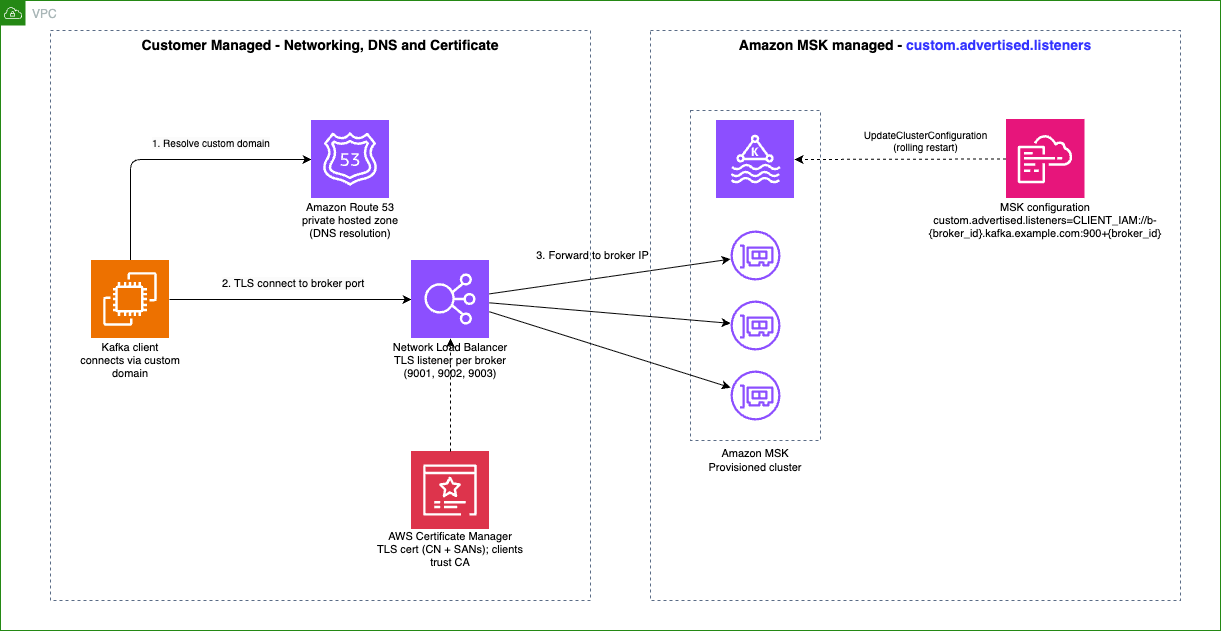
Figure 1: The client connectivity and trust layer (left) is a prerequisite you own and manage. The advertised listener configuration on the cluster (right) is what Amazon MSK manages for you
Important: When you apply
custom.advertised.listeners, your custom domain name replaces the default addresses that clients use to connect to broker nodes. If the networking and trust layer is not already in place, resolvable, reachable, and trusted from the client, the client cannot reconnect, even though it was connected moments earlier.
The Prerequisites section below shows the key requirements. You can find the detailed setup in an existing post, Configure a custom domain name for your Amazon MSK cluster, which includes a diagrammed walkthrough of the NLB, Amazon Route 53, and AWS Certificate Manager (ACM) topology.
After the connectivity layer exists, you tell the brokers which custom address to advertise to clients. This is the part that used to require a per-broker CLI override, and it is what this launch simplifies. This next section describes how it works.
Before a client can reach your brokers through a custom domain, the connectivity and trust path must exist. You create and manage this layer. It covers three things:
This layer must be in place for custom domain names to function. It is a prerequisite for this feature to work.
You add a property to your Amazon MSK configuration. The value takes the form:
where <LISTENER> is one of your cluster’s client listeners and <hostname>:<port> is the custom address pattern. For example, on an IAM cluster:
The property specifies two things:
CLIENT, CLIENT_SECURE, CLIENT_SECURE_PUBLIC, CLIENT_SASL_SCRAM, CLIENT_SASL_SCRAM_PUBLIC, CLIENT_IAM, and CLIENT_IAM_PUBLIC. Internal listeners (REPLICATION, CONTROLLER) are not supported and are rejected at validation. The listener you specify must also be bound (active) on your cluster. For example, if your cluster uses only IAM authentication, specifying CLIENT_SECURE is rejected, and the error message lists the valid client listeners for your cluster.hostname:port pattern that includes the {broker_id} template variable. Each broker resolves to a unique address. In this pattern, the {broker_id} template variable is replaced with each broker’s numeric ID. The port number 9000+{broker_id} means the broker ID is added to the base port 9000, so broker 1 resolves to 9001, broker 2 to 9002, broker 10 to 9010, and so on. The base port 9000 is only an example. You can use any base port, as long as the resulting ports match the TLS listeners you provisioned on your NLB.
{broker_id}can appear in the hostname, the port, or both, as long as each broker’s resolvedhost:portis unique. Placing it in the port alone is valid, so a shared hostname with a per-broker port also works:
Before you begin, you need an MSK configuration to hold this property. You create one with the CreateConfiguration API (or the AWS Management Console), passing your server properties as the configuration body. MSK returns a configuration ARN and a revision number, which together identify the exact configuration you apply to the cluster.
custom.advertised.listeners does not need its own standalone configuration. You can include it alongside any other broker-level properties MSK already supports, such as auto.create.topics.enable, num.partitions, or log-retention settings, within a single configuration revision. If you already manage an MSK configuration for your cluster, add custom.advertised.listeners to it and create a new revision using the UpdateConfiguration API. No separate configuration is needed.
You then apply the configuration to your cluster with the UpdateClusterConfiguration API. Amazon MSK then performs three actions:
These safeguards prevent you from accidentally removing or modifying the internal listeners that Amazon MSK manages. Validation is synchronous. The listener must be a client-facing listener, the pattern must include {broker_id}, and each broker’s resolved host:port must be unique. If any check fails, the API returns a descriptive error and makes no change.
The override affects only the advertised address of the named listener. Replication, authentication, multi-VPC (CLIENT_IAM_VPCE), and AWS PrivateLink connectivity remain unaffected. The change is also fully reversible: remove the custom.advertised.listeners property and re-apply the configuration, and Amazon MSK reverts the listener to its original address.
You can track progress with the DescribeOperation API, which shows state transitions from UPDATE_IN_PROGRESS to UPDATE_COMPLETE or UPDATE_FAILED. If a broker fails to start, the rollout halts at that broker, the remaining brokers keep their previous configuration, and you can fix the property and re-apply to recover.
When you apply custom.advertised.listeners, your custom domain name replaces the default addresses that clients use to connect to broker nodes. If the networking and trust layer is not already in place, resolvable, reachable, and trusted from the client, the client cannot reconnect, even though it was connected moments earlier.
The networking layer, the Network Load Balancer (NLB), DNS, and TLS certificate that route traffic from your custom domain to your broker IPs, is a prerequisite you own. It is not specific to this launch. The existing post Configure a custom domain name for your Amazon MSK cluster covers it in detail, with a diagrammed walkthrough of the NLB, Route 53, and ACM topology. With the networking in place, the following steps cover the cluster-side setup this launch introduces.
Create or update an Amazon MSK configuration that includes the custom.advertised.listeners property, matching the hostnames and ports you provisioned on the NLB. For a three-broker IAM cluster fronted by an NLB with ports 9001–9003, put the property in a file:
Then create the configuration, passing the file as the server properties:
Use fileb:// (not file://) so the CLI reads the file as bytes and base64-encodes it. Passing the value inline is fragile because of the {broker_id} braces. Leave {broker_id} literal in the file. Amazon MSK resolves it per broker at apply time. The response returns the configuration ARN and LatestRevision.Revision, which you use in the next step.
Apply the configuration to your cluster with UpdateClusterConfiguration, using the console, AWS Command Line Interface (AWS CLI), AWS CloudFormation, CDK, or Terraform. This is the same workflow you already use for broker configuration changes.
If the configuration fails to apply, review the errors. For details, see the troubleshooting section in the Amazon MSK Developer Guide.
After the configuration is accepted, Amazon MSK applies it through a rolling restart. Wait until the operation reports SUCCESS. If it reports FAILED, a broker could not apply the change. The rollout halts at that broker, the remaining brokers keep their previous configuration, and you can fix the configuration and re-apply to recover.
Confirm clients can connect through the custom domain:
If your topic list is returned, clients are successfully connecting through your custom domain. If the operation reported SUCCESS but clients cannot connect, the cluster-side configuration is correct, but your networking layer likely needs attention.
This step is important. Clients can be disconnected if the networking is not ready. Kafka clients do not keep using the original address they bootstrapped with. On a periodic metadata refresh, each client learns the broker’s advertised listener. The client uses that address for all subsequent connections. When you apply a custom domain name, that advertised address changes from the default name that Amazon MSK generates to your custom domain, so at the next metadata refresh every client connects over the custom domain. For this reason, the connectivity and trust layer described in What you set up, and what Amazon MSK manages is a prerequisite, not a follow-up task.
The safe sequence, which is also how customers move from Amazon DNS to a custom domain today, is two phases:
custom.advertised.listeners changes what the brokers advertise. At the next metadata refresh, clients pick up the custom domain and cut over to it automatically.Because the path already exists, this cutover is transparent: as Amazon MSK applies the change broker by broker, clients reconnect on their own, with no restart or reconfiguration.
When you scale the cluster or a broker is replaced during automated healing, Amazon MSK automatically applies the configuration to the new broker, resolving {broker_id} for its ID, with no manual steps required on the cluster side. Remember to add the corresponding NLB listener, target group, and DNS record for any new broker, because the networking layer does not auto-scale.
Custom domain name configuration turns a per-broker CLI workaround into a single, validated, cluster-wide Amazon MSK configuration property. It works identically on ZooKeeper and KRaft, persists through scaling and failover, and flows through your existing Terraform, CloudFormation, and CLI workflows. If you rely on custom domain names, we recommend adopting the static configuration now.
This capability is available on all Amazon MSK Provisioned clusters with Standard and Express brokers, in all AWS Regions where Amazon MSK Provisioned is available. To get started, see the Amazon MSK Developer Guide and the end-to-end networking walkthrough in Configure a custom domain name for your Amazon MSK cluster.
Post Syndicated from LastWeekTonight original https://www.youtube.com/watch?v=GQwFXp1uYuw
Post Syndicated from Bryton Herdes original https://blog.cloudflare.com/rfc9234-bgp-role-model/
Route leaks push traffic down paths it was never meant to take. We have written and spoken publicly in the past about route leaks in Border Gateway Protocol (BGP), depicting these events as impactful incidents that cause misdirection of traffic through unintended network paths. BGP routing is driven by the relationships between Autonomous Systems (ASes), i.e., customer-provider and peer-peer. Customers pay providers for access to the rest of the Internet, while peers exchange traffic with one another typically under a “settlement-free” arrangement where no money changes hands. These relationships help define routing rules that form plausible paths. For example, the rules form a “valley-free” hierarchy of how routes should propagate: a route learned from a provider or a peer should be announced only downward to customers, never back up to another provider or peer. Rules like this express an intent or expectation about Internet routes. A route leak is what happens when that intent is violated.
Historically, each network has had to implement this intent on its own, using complex, error-prone routing policies. RFC 9234 (Route Leak Prevention and Detection Using Roles in UPDATE and OPEN Messages) simplifies this by expressing intent within the protocol itself. It introduces a new “BGP Role” capability, which requires that two BGP neighbors agree on their relationship when the session comes up, and an “Only to Customer” (OTC) path attribute, which marks routes that must not propagate beyond customers. A router that understands OTC can reject a leaked route on its own, without an operator-written policy.
We set out to evaluate how well RFC 9234 works on the Internet and how widely it has been adopted. Relying on our global peering presence, we developed a unique method for tracking the adoption of BGP Role configurations by monitoring which peer ASes send the OTC attribute to Cloudflare. Along the way we found something we did not expect: two large Tier-1 networks strip the OTC attribute from routes they forward. We have been engaging with these Tier-1s to allow OTC attribute propagation through their networks, which aids in enabling route leak prevention capabilities for early adopters of RFC 9234. Below, we walk through our analysis, why the OTC stripping matters, and how to enable BGP Roles in your own network.
Before the measurements, let’s talk about how BGP Roles and the OTC attribute actually work.
Route leaks are the “propagation of routing announcements beyond their intended scope,” as defined in RFC 7908. The intended scope is determined by AS relationships: provider-to-customer or peer-to-peer.
The rules are asymmetric, and it comes down to direction. Routes propagate freely downward: a provider may hand a customer anything in its table. Propagating routes upward or sideways is restricted to ‘local’ information. Specifically, an AS may send in the upwards or sideways directions only the routes it originates and that are learned from its own customers.
The figure below shows what B does with a route it learns from A, depending on A’s relationship to B.
Putting it simply, a route leak happens when an AS takes a route learned from a provider or a peer and announces it to another provider or peer. The route travels down the hierarchy and then back up, creating a “valley” in the hierarchy that the underlying relationships never authorized. Routing paths are required to be valley-free.
Violations of the valley-free property come in many forms. A common shape is a customer announcing a route between two of its providers, also known as a hairpin turn.
This scenario is bad for everyone: the customer (AS64504) is not being paid to send traffic between its providers, and it also may not have the capacity to absorb the traffic flowing between the two upstream networks, resulting in increased latency or drops.
Route leaks impact everyone, and they happen often. That’s why we built the Cloudflare Radar route leak detection system to help track routing anomalies continuously. However, despite the frequency and the impact, existing defenses put the burden on network operators who must rely on prefix filters and IRR-derived policies. Such mechanisms require every AS to express its own relationships correctly, by hand, on every session. RFC 9234 moves that burden into the BGP routing protocol.
A BGP Role declares where you sit relative to a neighbor on the given eBGP (External BGP) session. The Role describes each side of the neighbor relationship: on a session with your transit provider, you configure the Role customer, and they configure the Role provider.
There are five options: Provider, Customer, Peer, RS, and RS-Client. The first three are the transit and lateral-peering relationships described above. RS and RS-Client involve Internet Exchange (IX) route servers, where a route server acts like a provider to all of its clients, re-announcing prefixes between IX members transparently.
Only five pairings of the five roles are valid:
RFC 9234 states a Role should be configured at the local AS on every eBGP session. During partial deployment, most sessions will have a Role on one side only. RFC 9234 handles that by default: if you send the Role capability and your neighbor does not, the session still comes up, and your locally configured Role still drives partial route leak prevention. An operator who wants a stronger guarantee can enable "strict mode," which rejects any session where the neighbor sends no Role capability. Strict mode is opt-in, and as the adoption numbers later in this post show, it is not yet realistic for most networks.
When both sides send a Role and the pair is not one of the five above (e.g., one end says customer and the other says peer), the session is rejected with a Role Mismatch notification (code 2, subcode 11).
The rejection is one reason Roles are so useful: a Role mismatch means the two networks disagree about what their relationship actually is, which is precisely the kind of latent misunderstanding that surfaces later as a route leak. A Role mismatch fails the handshake instead of failing later as an incident.
No single Role is able to describe multiple roles, for example, if you hold more than one relationship with the same neighbor over a single session (e.g., provider-to-customer for some prefixes, peer-to-peer for others). RFC 9234 says Roles must not be configured on such a session at all. Instead, networks need to split the Complex relationship into separate eBGP sessions with normal relationships, and configure the relevant Role on each. Without individual sessions that are assigned Roles, a network operator must implement a more complicated per-prefix policy with no in-band way to check that the policy is correct — which falls back to the failure-prone ‘by-hand’ mechanisms that motivate Roles in the first place.
Roles have a second use beyond session negotiation. In our earlier post on ASPA validation, we described how a different algorithm applies to paths received from a provider than to paths received from a peer, customer, route server, or route server client. Routes from a provider may contain a full upward, sideways, and downward motion in the path. However, routes from a non-provider must only contain a downward-facing ramp to customer ASes.
The BGP Role is what tells the router which of the two to run, so BGP Roles and ASPA should be configured together on routers that support both.
OTC is an optional transitive path attribute (type code 35) carrying one value, an AS number. That value records the AS that first sent the route sideways or downward. It marks the peak of the path, after which the route may only continue down. Once OTC has been set, RFC 9234 requires it to be preserved unchanged. And because the attribute is optional transitive, even a router with no RFC 9234 support is expected to pass it along rather than discard it. Both of those facts matter later.
Your Role on each session decides which rules apply.
Setting OTC. A route is stamped the first time it stops travelling strictly upward:
Checking OTC. Once a route carries OTC, it may only travel downward:
As a concrete example, let’s return to the hairpin leak, but add Roles and OTC. AS64502 announces the route to its peer AS64503, attaching OTC=64502 on the way out. AS64503 passes it further down to its own customer AS64504, while leaving OTC untouched because it is already present. AS64504 then unintentionally violates the intended BGP relationships, by announcing the route to its other provider.
OTC has two opportunities to stop the leak. If AS64504 is compliant, it must not announce an OTC-carrying route to a provider at all, and the leak never leaves. If AS64504 is not compliant, as shown in the above example, the receiving provider sees a route arriving from a customer with OTC attached, which RFC 9234 defines as a leak, and marks it ineligible. Either alone is enough.
In summary, configure a Role on eBGP sessions, and you automatically get route leak protection in BGP.
As mentioned above, RFC 9234 outlines the rules for setting OTC both on egress and ingress routes. In an ideal world with complete (and correct) deployment, egress OTC attachment is enough. However, in the case of partial deployment or misconfigurations, ingress stamping by the receiving RS-Client, Customer or Peer fills in the missing OTC value. Quoting the relevant rule of RFC 9234 section 5 directly:
If a route is received from a Provider, a Peer, or an RS and the OTC Attribute is not present, then it MUST be added with a value equal to the AS number of the remote AS.
While this double-sided OTC attachment serves to tag as many routes as possible, it also obfuscates who has set the OTC value. For example, by observing the path 64506 64507 with OTC=64507, we cannot infer whether AS64507 set the OTC on egress or AS64506 set its missing value on ingress.
This makes identifying adopters of RFC 9234 by tracking OTC difficult, but is important enough for us to try.
With this limitation in mind, we first attempted to detect which ASes are setting the OTC value by analyzing the Routing Information Base (RIB) dumps of all public BGP collectors from RouteViews and RIPE RIS. While naively counting the distinct OTC values gives us 361 potential setter ASes, this number is inflated by ASes filling in missing values from their peers, providers, and, less frequently, RSes. To account for this, our first step was to count the number of OTC values that were equal to the first AS of the AS_PATH. Those ASes set the OTC attribute towards the route collectors which capture the raw received BGP messages. This step gives us an initial number of nine setter ASes.
Extending this analysis to detect if OTC was set on egress or on ingress in the AS_PATH requires using multiple guards to differentiate. We started with a simple and relaxed method to estimate the ASes potentially setting the OTC. We looked at all the AS_PATHs with an OTC value, and collected all the edges (ASX ASZ) where OTC = ASZ. Then, based on these edges we created two mappings, downstream: ASN→next_hops and upstream: ASN→previous_hops. For example, in the case of (ASX ASZ), we would add ASX to downstream(ASZ) and ASZ to upstream(ASX). As a next step, we want to remove from both sides the ASes that with higher confidence are setting OTC on the other side. For that, we collect all the ASes Y that have |downstream(Y)| ≥ 10 or |upstream(Y)| ≥ 10, and then remove them from the previous_hops or next_hops respectively.
As a final step, out of those two mappings we kept the ASes with at least three next or previous hops, and found 18 ASes potentially setting OTC and 20 ASes potentially filling in missing OTC values in the ingress. Combining these results with the ones from direct peer ASes, we find only 36 ASes that are potentially RFC 9234-compliant, although the true number needs further investigation.
We understand that for the sake of certainty this method may miss ASes that have very few downstreams or upstreams. We are already looking at improvements. For example, AS_PATHs missing the OTC value may be negative evidence for an AS not setting OTC. In this approach, knowledge of the relationships between the ASes is necessary to focus only on instances where OTC should be set, i.e., not in upstream direction. However, getting accurate AS relationships has been a hard problem for over two decades, but multiple efforts exist that may be helpful such as CAIDA’s and BGPKIT’s AS Relationships datasets. Public data is invaluable, even with inherent shortcomings.
We decided to supplement the view of RFC 9234 compliance by devising experiments conducted using Cloudflare’s network, in service of and spirit of an open and public Internet.
Cloudflare, with thousands of peers and an open peering policy, can help track who has implemented RFC 9234. As we described before, the core challenge is how to confidently differentiate whether OTC was set on egress or on ingress. Since Cloudflare peers directly with many ASes, we can assess their RFC 9234 compliance directly, without the ambiguity introduced by intermediate ASes.
Our methodology is simple and concrete: we use our BMP (BGP Monitoring Protocol) feeds from our routers at Cloudflare to monitor OTC that we receive from our peers. We check if the OTC value is equal to the peer ASN. We processed our BMP data over the past three months and found 67 ASes that set the OTC attribute. In the figure below, we show a distribution of the network types of those ASes according to PeeringDB with some manual corrections.
Two features of the pie chart stand out. First, we observe how Route Servers are more likely to quickly adopt new solutions such as RFC 9234 with YYCIX being the first to deploy it, partially due to the use of open-source BGP implementations that introduce new features much faster. This is very important as Route Servers play a critical role in the public Internet; they sit in the path of propagation of numerous routes and, by adding the appropriate OTC value, help protect a significant part of the Internet. We hope to see more and more RSes following this example. Second, the proportion of compliant ASes owned by individuals features highly. One explanation may be personal inclinations to use open-source BGP implementations.
Shown below is our current view of RFC 9234 adoption by observing OTC from peers over the past three months.
Looking ahead, we will keep a close eye on the adoption of RFC 9234 by tracking OTC, and plan to release this data publicly in Cloudflare Radar’s Routing section in the near future. In the meantime, we wondered which networks may unexpectedly strip the OTC attribute.
According to RFC 9234, OTC is an optional transitive attribute. Section 5 of RFC 4271 states the following about handling optional transitive attributes:
Paths with unrecognized transitive optional attributes SHOULD be accepted. If a path with an unrecognized transitive optional attribute is accepted and passed to other BGP peers, then the unrecognized transitive optional attribute of that path MUST be passed, along with the path, to other BGP peers with the Partial bit in the Attribute Flags octet set to 1.
Before RFC 7606, the propagation of a malformed transitive attribute would remotely trigger multiple session resets, and cause outages far away from the AS that originated the announcement. This makes sense since, if a BGP speaker received a BGP UPDATE with a malformed attribute, it would reset its session with the neighbor that sent the message. This vulnerability motivated some operators to start dropping unrecognized attributes, even if transitive, in order to minimize the impact of such a misconfiguration or an attack. There was even a recent issue where a malformed OTC attribute caused session resets in some BGP implementations. RFC 7606 addressed this risk by defining finer-grained error-handling where an announcement with a malformed optional attribute would cause to "treat-as-withdraw" the prefixes in it, while the session is preserved.
Propagating OTC even if unrecognized is vital for RFC 9234-compliant ASes that are multiple hops away to detect and prevent route-leaks. In early partial deployment stages, central or top-tier ASes bear the responsibility of adopting such routing security solutions, or at least not compromising their effectiveness by stripping essential attributes.
We wanted to study who is stripping the OTC attribute on the Internet. In our experiment, we announced one IPv4 and one IPv6 prefix, with attached OTC = 13335, from all of our peering locations using BGP Anycast. After confirming global propagation, we later withdrew the prefixes to trigger the path hunting process, revealing more paths to the test prefixes, giving us more opportunities to spot OTC-absent paths. As shown in the figure below, we used the BGPKIT toolkit to parse the Update messages from the Multi-threaded Routing Toolkit (MRT) dumps of all the public BGP collectors from RIPE RIS and RouteViews, and the local BMP data that we collect from our routers. Note that we opted to analyze the Updates instead of the Routing Information Base (RIB) dumps, which are snapshots of the routing tables of the peer ASes, to retrieve as many routes as possible both during the announcement and the withdrawal phase.
First, we focused on the AS_PATHs in the format ASX AS13335. If that path does not carry an OTC value, ASX must have stripped the attribute. With this first step, we found six ASes dropping OTC, out of which two were Tier-1 ASes, AS3257 (GTT) and AS1299 (Arelion). Moving forward, we iteratively looked at longer paths to build two distinct sets of ASes preserving the OTC value and ASes dropping it:
Our methodology yielded nine more ASes that are dropping the OTC value. Additionally, we counted the number of distinct AS_PATHs that carried no OTC and found that 33.1% of routes for IPv4 and 17% for IPv6 had their OTC attribute dropped. This means that despite the possibly small number of ASes scrubbing OTC, almost one out of three AS_PATHs in IPv4 had its OTC stripped.
We first focused on the impact of two Tier-1 ASes, AS1299 and AS3257, due to their prominent position on the Internet. In the figure below, we show the proportion of OTC-absent AS_PATHs that included either or both of the two Tier-1s. Together, they appear in 96.6% of IPv4 and 92.9% of IPv6 OTC-absent paths, though Arelion accounts for the vast majority of these instances.
Additionally, when we concentrated on the AS_PATHs where the next hop of AS13335 is either of those two Tier-1s, we observed that while GTT was consistently dropping the OTC attribute, Arelion had 71.4% in IPv4 and 40.7% in IPv6 of those AS_PATHs without an OTC. This meant that Arelion inconsistently dropped the OTC across their network. These findings highlight the critical role high-tier ASes play in the deployment of RFC 9234.
We contacted both GTT (AS3257) and Arelion (AS1299) with our research findings, and they confirmed they were indeed stripping the OTC attribute as a part of defensive practices following BGP error-handling incidents of the past.
Current configurations at GTT (AS3257) still result in the OTC attribute being removed. This will continue to hinder the effectiveness of RFC 9234 against route leaks propagating through AS3257 until they preserve the OTC attribute and/or configure BGP Roles on their routers.
In the case of Arelion, it appears they rolled out configurations to begin preserving the OTC attribute soon after our conversation. We can verify that OTC is no longer missing from paths through AS1299 with our experiment prefixes using monocle. Here is an example query:
We are very excited that our research has already resulted in better effectiveness for route leak prevention using the OTC attribute.
The BGP Role configuration and OTC attribute are critical building blocks for preventing route leaks from propagating and causing major incidents. The table below lists the BGP implementations that already support these configurations or have planned to support RFC 9234 soon as of August 2026:
If your routing vendor already supports RFC 9234, we recommend that you configure Roles now to start preventing route leaks. Keep in mind the rollout will need to be completed during maintenance windows, as BGP sessions will need to be reset upon applying Roles. At Cloudflare, we have already started our gradual deployment of RFC 9234 configurations across our global fleet of routers.
Compared to complex routing policy configurations, route leak prevention provided by the Only to Customer attribute is automatic once the Roles are applied.
If your vendor does not yet support RFC 9234, we encourage you to reach out to them and ask for support, so you can prevent your network from spreading or initiating leaks as soon as possible.
Post Syndicated from LGR original https://www.youtube.com/watch?v=H9MPO0ZeDbI
Post Syndicated from Channy Yun (윤석찬) original https://aws.amazon.com/blogs/aws/in-the-works-aws-builder-lofts-in-berlin-hyderabad-and-sao-paulo/
In the early days of cloud computing, AWS supported intensive learning for builders in a physical space called the AWS Pop-up Lofts in cities worldwide. These spaces were accessible to startup entrepreneurs, developers, and others interested in learning more about AWS for events, meetings, and co-working. With the recent emergence of generative AI, AWS Gen AI Lofts provided pop-up style collaborative spaces across the world and immersive experiences for startups and developers.
We realized the need of permanent community spaces give students and developers a place to learn, connect, and contribute through hands-on experiences, community-led sharing, and technical collaboration. Since opening in San Francisco in July 2025, the first AWS Builder Loft has welcomed more than 22,500 developers through its doors, hosting hackathons, workshops, demo nights, and community-led events that bring the local tech community together under one roof.
Today, we are announcing plans to open new Builder Lofts in Berlin, Hyderabad, and São Paulo. Each location will be a permanent community space to offer free workshops, networking events, pitch nights, content creation spaces, collaboration/co-working areas, and event hosting for developers, students, or tech professionals who want to walk through the doors.
You’ll still be able to meet AWS experts there, but beyond that we further want to establish a home for local tech communities from AWS User Groups and AWS Student Builder Groups, to independent developer groups you’re already part of. As a tech community leader, you are welcome to request booking of our space to host your meetup at no cost.
Why three cities
The expansion reflects fast-growing developer cities which are important talent and innovation hubs for each region:
A typical week at the Builder Loft
The Builder Loft in San Francisco hosts four to eight community events weekly from technical deep dives on generative AI to startup pitch nights, from coding workshops for students to networking sessions that bring together developers from across the region.
The spaces are designed to be flexible. A training room fills with over 50 students on a Tuesday morning. By evening, it transforms into a demo stage where a startup showcases its latest prototype to a room of potential collaborators. On weekends, community groups host their own meetups.
What makes the model work is that it’s driven by the community itself. Local developers, meetup organizers, and tech leaders shape the programming. AWS provides the space, the infrastructure, and the support, but the energy comes from the builders who participate. Find upcoming events or request to host your own event at the Builder Loft San Francisco.
Stay tuned
We’ll announce Builder Loft openings in three cities in future blog posts, so stay tuned for updates! To learn more about Builder Lofts for details and to follow along for updates, read Rick’s blog post and visit the AWS Builder Loft page.
— Channy
Post Syndicated from jzb original https://lwn.net/Articles/1088489/
The Linux kernel’s user-space interface
(AF_ALG) to the Crypto
API has been linked to a number of recent high-profile security problems,
including Copy Fail and successor
vulnerabilities. It was deprecated
earlier this year. Eric Biggers, and other kernel developers,
have been working to remove it
from the kernel. With that in mind, the Fedora Project is planning to
restrict use of AF_ALG in the next Fedora release in the hopes of nudging
remaining users of the API to prepare for its eventual removal.
Post Syndicated from jzb original https://lwn.net/Articles/1089338/
Security updates have been issued by AlmaLinux (.NET 8.0, 389-ds:1.4, bind, haproxy, kernel, kernel-rt, libXfont2, nghttp2, and unbound), Debian (calibre, expat, ironic, and linux-6.12), Fedora (coturn, linux-firmware, php-phpseclib, and sqlite), Red Hat (fence-agents, osbuild-composer, pam, resource-agents, and sg3_utils), SUSE (ffmpeg, jetty-minimal, open-iscsi, python, python313-h2, python313-pysaml2, redis, redis7, rsync, sccache, texlive, and wasm-bindgen), and Ubuntu (engrampa, linux-aws-7.0, and linux-azure-fde-5.15).
Post Syndicated from Rapid7 Labs original https://www.rapid7.com/blog/post/tr-new-report-ai-threats-q2-2026-ends-traditional-patch-cycles
You can’t patch everything. So what do you fix first? Findings in Q2 2026 have changed traditional answers.
The latest Quarterly Threat Landscape Report from Rapid7 Labs shows vulnerability disclosures still surging while attackers use automation and AI-assisted tooling to compress the time between disclosure and exploitation. The gap that patch cycles were built to fill is closing. Speed and volume are overwhelming security teams that have relied on traditional patch cycles and reactive programs. Success going forward can’t be about patching as much as possible – it has to be about understanding what matters most and reducing the exposures attackers can actually reach.
Here are the four trends that defined Q2 2026, and what they mean for your security program as you define priorities for Q3 and beyond:
There were 8,539 new high- and critical-severity CVEs (CVSS 7.0–10.0) this quarter- double the number reported in the same quarter last year (4,268). Meanwhile, the number of newly exploited vulnerabilities held roughly steady (40). The takeaway isn’t that exploitation exploded – it’s that disclosure volume is far outstripping what any team can triage.
The report breaks down which of those disclosures are actually reachable and how to triage by exploitability instead of severity score alone.
Nearly two-thirds of exploited vulnerabilities this quarter (62%) required no user interaction – no stolen credentials, no phishing victim, no click. Attackers reach and exploit them on their own, and that share is up nine points year over year (from 53% in Q2 2025). Reinforcing the trend, disclosures of missing-authentication flaws (CWE-306) surged 247% year over year – a fast-expanding pool of internet-facing systems that require no login at all.
This is the quarter’s clearest signal – and the report details exactly which exposures to close first, and how, before the exploitation curve catches up.
Rapid7 observed continued activity from Iranian, North Korean, and Russian advanced persistent threat (APT) clusters targeting government, finance, healthcare, manufacturing, energy, and telecommunications. Russian campaigns targeted edge infrastructure; Iranian activity included sustained industrial control system (ICS) and operational technology (OT) targeting.
The report maps the specific techniques and sectors each cluster focused on this quarter.
Qilin led ransomware activity in Q2 with 263 listed victims, and the United States remained the most heavily targeted country – with business services and healthcare among the hardest-hit sectors. Rapid7’s Incident Response team also saw growing use of ClickFix and fake CAPTCHA campaigns, and social engineering through trusted collaboration platforms like Microsoft Teams – techniques that accounted for 31.8% of the incidents we worked.
The report includes the full ransomware leaderboard, the sectors most at risk, and where affiliate activity is expanding next.
The volume is daunting, but the real challenge is keeping pace with attackers. As disclosures keep growing, the organizations that stay ahead won’t be the ones patching fastest — they’ll be the ones that know what they expose, which assets matter most, where attackers can realistically get in, and how to reduce reachable exposure before it becomes an incident. That’s what preemptive security means: not a slogan, but an operating model.
The full Quarterly Threat Landscape Report shows where reachable exposure concentrates this quarter, the four actions Rapid7 Labs recommends, the sector-by-sector breakdown, and the dark-web signals shaping what’s next. Read it here before you pressure-test your Q3 prioritization.
Post Syndicated from The History Guy: History Deserves to Be Remembered original https://www.youtube.com/watch?v=qy16rKjWRCc
Post Syndicated from Suman Chatterjee original https://aws.amazon.com/blogs/architecture/consistency-is-the-new-latency-ai-at-the-data-layer/
As AI applications scale from reactive bots to autonomous agents, their reliability is bound to the speed and accuracy of the data layer beneath them.
There’s a quiet assumption baked into most AI architectures today regarding data layer consistency, and it’s costing companies more than they realize. The assumption is that the data your AI agent reads is the current state of reality.
In a world of distributed systems, cross-region replication, and autonomous agents making millisecond decisions, this assumption breaks down.
I’ve spent extensive time working with enterprise teams building agentic AI, and a recurring failure pattern emerges.
The breakdown isn’t in the model or the prompts. It’s in how we manage replication consistency when an agent performs the reading.
In a modern agentic Retrieval-Augmented Generation (RAG) architecture, the database is the active memory of your AI. When an agent performs a task, it retrieves data to build its context window, forming the foundation of the large language model’s (LLM) reasoning.
If that data is even slightly out of date, the agent’s entire reasoning chain is invalidated. We must shift from simply managing data availability to strictly verifying contextual integrity.
In traditional web applications, asynchronous replication scales global reads with minimal write impact. If a user sees a post 500ms late, nobody notices.
For an autonomous AI agent, a 500ms delay is silent poison. If an agent writes a decision to a primary node and immediately reads from a lagging replica, it treats stale data as ground truth. It then executes a logically coherent, multi-step plan based on factually incorrect inputs.
In the age of AI, a fast answer that is wrong is more expensive than a slightly slower answer that is right.
Consider an autonomous Inventory Reconciliation Agent managing a flash sale:
available_stock to 500 units on the primary database in us-east-1.ap-south-1 (Mumbai) replica.The agent didn’t make a reasoning error. It performed logical operations on poisoned context.
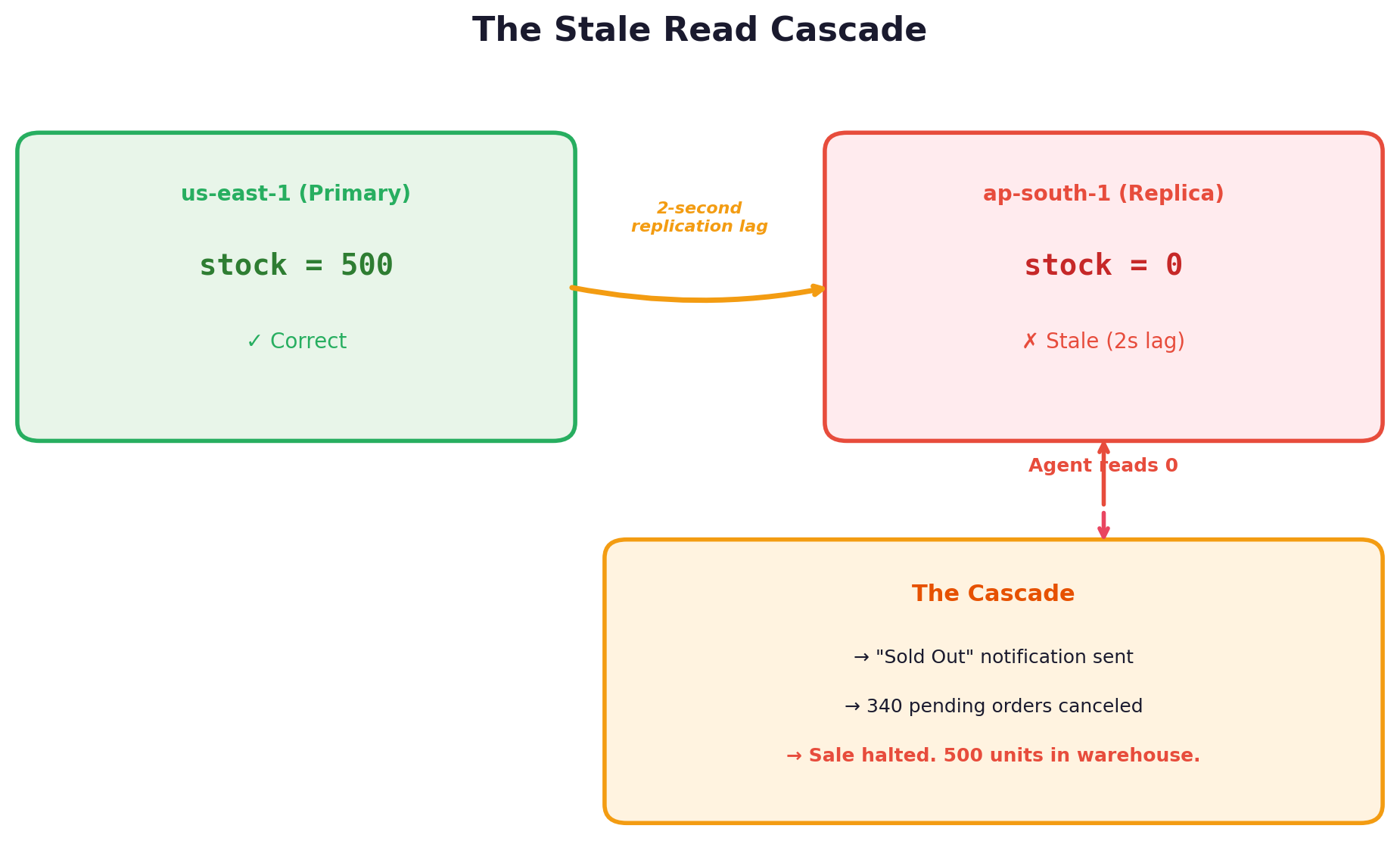
Figure 1: The stale read cascade, showing how replication lag poisons an AI agent’s context
When an agent writes an incorrect conclusion back to the database, that error becomes long-term memory. Future retrievals pull this poisoned history, creating a self-reinforcing cycle of “Hallucination Debt.”
LLMs amplify this because they lack a temporal compass. They cooperatively treat retrieved database results as current facts without hesitation. The burden of verifying contextual integrity falls entirely on the architecture.
Not all AI tasks have the same consistency requirements. You must match your replication model to the specific “truth requirement” of the task.
Here are three architectural patterns I’ve found most effective.
When an agent manages high-stakes data (user permissions, security policies, financial records, core system instructions), the cost of a stale read is unacceptable. You need strong consistency.
For many workloads, Amazon Aurora Global Database provides the necessary foundation. While its cross-region storage replication is asynchronous by default, you can close the consistency gap by turning on Global Write Forwarding with a GLOBAL consistency level.
To verify Read-Your-Own-Writes integrity, you configure the SESSION consistency level, which makes an agent wait for its own forwarded writes to replicate back before reading.
For the strongest consistency, the GLOBAL level makes a read query wait for replication to catch up to the exact point in time when the read started.
For the next generation of globally distributed AI, Amazon Aurora DSQL addresses this need. Aurora DSQL offers native synchronous strong consistency across multiple regions, so multi-agent systems can scale globally without compromising accuracy.
Every agent, regardless of location, operates on the exact same ground truth.
Best for: Identity metadata, financial ledgers, immutable system prompts.
Why it matters: Eliminates “mid-thought” state changes that cause contradictory behavior between agent instances.
For global AI agents that need ultra-low latency at massive scale, Amazon DynamoDB Global Tables offer a multi-leader architecture where data replicates across regions. For replication details, refer to the DynamoDB documentation.
The key technique here is Conditional Writes. By using a ConditionExpression that checks a version timestamp or whether an attribute exists, an agent updates a record only if the data hasn’t changed since it was last retrieved.
If the condition fails, DynamoDB returns a ConditionalCheckFailedException. This is a critical signal: it tells the agent to re-read the current state and reconsider its decision, rather than blindly overwriting another agent’s work.
This pattern prevents the “Lost Update” anomaly (where two agents running in parallel overwrite each other’s reasoning) without requiring synchronous global coordination.
Best for: Conversational history, user session state, personalized agent memory.
Why it matters: Handles concurrent updates from distributed agents while maintaining a shared memory that’s resilient to race conditions.
Some AI agents perform real-time anomaly detection or trend analysis on massive streams of telemetry data. In these cases, you need unthrottled ingestion above all else.
A leaderless architecture like Amazon Keyspaces (for Apache Cassandra) is designed for this workload.
Keyspaces provides highly available, predictable performance by automatically replicating data across three Availability Zones.
Every write is durably committed using LOCAL_QUORUM.
To make sure your AI agent doesn’t miss a critical spike in telemetry, you enforce strong consistency by setting its read operations to LOCAL_QUORUM rather than the eventually consistent LOCAL_ONE.
This quorum overlap means the agent retrieves the latest data without slowing down the high-speed ingestion pipeline.
It transforms a noisy, high-frequency data stream into a reliable foundation for real-time AI decision-making.
Best for: Internet of Things (IoT) telemetry, real-time log analysis, high-frequency sensor data.
Why it matters: Throughput is the priority, but you still need a safety valve to confirm the agent doesn’t miss critical spike data.
Our role as architects has evolved.
We can no longer treat database replication as a background infrastructure concern, something to configure once and forget. In the era of autonomous agents, the stability of the data layer is the direct prerequisite for the trustworthiness of the AI. The two are inseparable.
By matching your replication model to your agent’s reasoning requirements, you move beyond simply managing data. You become a Context Architect, someone who works to confirm that every decision your AI makes is grounded in a synchronized version of the truth.
Because in the end, an AI is only as good as the context it operates in. And context is only as good as the data it’s built on.
Get the database layer right, and everything else follows.
References: