Amazon Threat Intelligence observes threat actors running cybercrime campaigns with Artex AI agents

Post Syndicated from CJ Moses original https://aws.amazon.com/blogs/security/amazon-threat-intelligence-observes-threat-actors-running-cybercrime-campaigns-with-artex-ai-agents/

From Oct. 3 to Nov. 5, 2026, Amazon’s MadPot, a globally distributed network of decoy threat sensors, captured requests from AI agents that included operating memory from offensive campaigns that threat actors ran on ARTEX, an open-source agentic AI penetration testing framework. The ARTEX agents sent these requests to MadPot sensors configured to present as popular large language model (LLM) inference APIs, and the requests carried the agents’ own records of their campaigns.

Amazon Threat Intelligence assessed threat activity referencing potentially affected AWS customers and notified them as appropriate. Because activity against other organizations could not be confirmed, this post shares the findings and indicators of compromise (IOCs) so that organizations that run the affected technologies can review their own environments.

The most prominent ARTEX campaign was a large-scale theft of credentials to access AI models, organized as a self-sustaining operation in which stolen keys paid for the LLM inference powering further credential hunting. Another campaign targeted cryptocurrency exchanges for know-your-customer (KYC) verification bypass using real-time deepfake injection. In aggregate, the agent records show that agentic frameworks have progressed from experimental use to sustained, multi-objective offensive operations that run with minimal human intervention. This post describes how these campaigns operated based on the agents’ own descriptions of the campaigns.

Attribution and instructions

Amazon Threat Intelligence assesses with moderate confidence that ARTEX was used for these campaigns due to prompt references to ARTEX tooling and other technical artifacts referencing ARTEX. Threat actors instructed ARTEX agents through standing instruction prompts that set the mission objectives, targeting rules, and operational constraints. Within those instructions, the agents handled the work themselves. In one credential theft campaign, operators told the agents to work through a fixed sequence of countries, prioritize enterprise production sites over personal projects, and grade every stolen credential by whether it worked and what it could reach. Agents were directed to treat credentials exposed publicly for more than 30 days as low-value inventory.

Amazon Threat Intelligence also assess with moderate confidence these are disparate Chinese-nexus threat groups due to use of simplified Chinese language in prompts, China time-zone configurations, targeting consistent with Chinese interests, and tooling predominantly used by Chinese-nexus threats. Sample instructions included setting red lines, such as excluding mainland China targets and government domains, and required all outbound traffic to go through proxies.

How MadPot saw inside these campaigns

MadPot presents controlled services to potential attackers and records how they discover, test, and attempt to compromise or abuse them. MadPot telemetry allows Amazon Threat Intelligence to observe attacker behavior without exposing customer workloads. In this case, the MadPot sensors presented popular LLM-compatible chat-completions interfaces on various ports. Agentic frameworks sent prompts to these interfaces as part of their offensive workflows, treating them as LLM inference backends.

The resulting telemetry contained the persistent task context, system prompts, tool histories, knowledge-graph state, and reported findings that these frameworks ordinarily send to an LLM to make operational decisions. Because agentic frameworks retain the history of past conversations, individual requests often contain the full operational history of a campaign. That history described activity that occurred before and between the captured requests, on systems MadPot does not monitor. Amazon Threat Intelligence did not observe that activity as it happened and cannot verify the outcomes the agents reported, but the records show what the actors were pursuing.

Most of the activity used ARTEX to divide work among planner, worker, verification, and compression agents sharing a persistent knowledge graph. The knowledge graph acts as the operation’s shared memory: every agent reads from it, and writes its results back, so each agent picks up where the others left off. The agents’ records described reconnaissance, vulnerability testing, credential theft, cloud-privilege expansion, and cryptocurrency fraud attempts across hundreds of targets spanning AI application platforms and other workloads. These records show how threat actors are organizing persistent, financially motivated offensive operations using agentic AI frameworks.

Campaign 1: Stealing AI credentials at industrial scale

In this campaign, threat actors used AI agents to steal API keys and other credentials that grant access to AI models, most likely so they could use those models while someone else paid for them. The agents’ records show stolen keys being fed into the framework’s own model gateway, where they powered the agents searching for more keys. Beyond AI model access keys, cloud credentials were treated as a doorway to more access. Agents validated identities through each provider’s token and identity services, enumerated storage, assessed permission scope, and went after managed AI model services, secrets and parameter stores, and application identities. They prioritized access to premium frontier models over general cloud permissions.

Agents recorded use of different AI gateways, keys, and models, but they all used a shared method: find internet-exposed AI applications, extract the upstream provider keys they hold, validate those keys, and store them in a managed pool. The agents focused on applications that aggregate provider keys, because one weak management interface can expose many downstream accounts. Targets included LLM gateways and proxy platforms such as One API, New API, Veloera, Sub2API, and LiteLLM, and AI application builders such as Dify, FastGPT, Langflow, RAGFlow, Open WebUI, LobeChat, and Ollama. A codified vulnerability playbook mapped each fingerprinted product to its known attack chain, including uninitialized installs that could be claimed, anonymous management and provider-configuration endpoints, default administrator credentials, such as the LiteLLM default master key, CVE-2025-3248 (Langflow), CVE-2026-28797 (RAGFlow), an authentication bypass via the isCliRequest header in One API family systems, SSRF through URL-fetch features to cloud metadata services, and secrets left in client-side JavaScript, source maps, debug routes, and environment files.

To find those keys, discovery drew on internet scanning services, certificate transparency, and public code and artifact sources: GitHub repositories and event archives (targeting secrets that fell outside automated revocation), npm and PyPI tarballs, container image layers, notebooks, model-hosting spaces, paste sites, and Telegram channels. One parallel operation worked through a fixed country sequence, prioritizing enterprise production sites, and graded every credential: L1 for a lead, L2 for a confirmed working API call, and L3 for quantified impact, such as readable data or spendable balance. Keys exposed publicly for more than 30 days were treated as low-value inventory.

Campaign 2: Defeating identity verification with deepfakes

In this campaign, threat actors used AI agents to defeat the identity verification (KYC) checks at two cryptocurrency exchanges with deepfakes. The agents’ records show generating real-time deepfake video to pass live selfie checks and forged ID document photos to pass document checks.

The records describe a methodical approach to the liveness check, which is a security method that confirms a person interacting with a digital system is a real, living human being physically present at the time of capture. The agents reverse-engineered one vendor’s liveness protocol in detail, documenting the face-detection event stream it sends, how it tracks face position during the check, and the coordinate system it uses to tell the user where to move. Their best recorded attempt completed the full movement sequence with the face positioned within 7 pixels of the target. Even so, the vendor’s server-side verdict rejected the deepfake in every attempt the agents recorded. In parallel, a separate session built a real-time deepfake video pipeline on a single consumer-grade GPU using an open-source face animation model. By splitting the model and avoiding unnecessary memory copies on the GPU, it reached 11.5 frames per second, close to what a live video check expects.

The agents worked on the ID document as well. Verification vendors look for signs that a document photo was edited or is a picture of a screen rather than a camera capture. To get past those checks, the agents recorded building synthetic camera metadata whose image dimensions matched the real values inside the JPEG file, and preserving the original camera compression tables that re-saving an edited image would normally replace. The result is an altered image that looks, at the file level, like an untouched camera photo.

This campaign also shows how ARTEX runs several workstreams toward one goal. At least four agent sessions ran at once: one searched for ways to cash out, one worked on clearing account balances, one set up the deepfake video pipeline, and one carried out the verification bypass. They shared findings and handed off tasks through cross-session tools.

What this means for defenders

None of the techniques in these campaigns were new. What AI agents change is the speed and persistence of the attacker. The agents succeeded where basic security hygiene was missing, including default or hardcoded credentials, keys left in code and public artifacts, unauthenticated interfaces and inference endpoints, and unpatched software. Getting those fundamentals right remains the most effective defense.

Given the speed and persistence of the attackers, organizations should assume exposed secrets and misconfigurations will be found quickly and remediate accordingly. They should bring AI applications, model gateways, and inference endpoints under the same controls as other production systems, and they should watch for misuse of AI services through unexpected spend or unusual usage.

Indicators of Compromise (IOCs)

IOC Value IOC Type First Seen Last Seen Annotation
104.28.225[.]223 IPv4 2026-10-17 2026-10-19 Campaign 1
31.22.91[.]156 IPv4 2026-10-14 2026-10-19 Campaign 1
150.136.38[.]110 IPv4 2026-10-31 2026-10-31 Campaign 1
128.242.115[.]131 IPv4 2026-10-31 2026-10-31 Campaign 1
216.176.239[.]231 IPv4 2026-11-02 2026-11-02 Campaign 1
212.107.28[.]51 IPv4 2026-10-14 2026-10-14 Campaign 2
103.142.140[.]158 IPv4 2026-10-17 2026-10-17 Campaign 2
104.28.251[.]98 IPv4 2026-10-18 2026-10-18 Campaign 2
104.28.251[.]99 IPv4 2026-10-18 2026-10-18 Campaign 2
104.28.219[.]97 IPv4 2026-10-18 2026-10-18 Campaign 2
125.103.213[.]41 IPv4 2026-10-18 2026-10-19 Campaign 2

If you have questions, start a new thread on AWS re:Post or reach out to AWS Support.

CJ Moses

CJ Moses

CJ Moses is the CISO of Amazon Integrated Security. In his role, CJ leads security engineering and operations across Amazon. His mission is to enable Amazon businesses by making the benefits of security the path of least resistance. CJ joined Amazon in December 2007, holding various roles including Consumer CISO, and most recently AWS CISO, before becoming CISO of Amazon Integrated Security September of 2023.

Prior to joining Amazon, CJ led the technical analysis of computer and network intrusion efforts at the Federal Bureau of Investigation’s Cyber Division. CJ also served as a Special Agent with the Air Force Office of Special Investigations (AFOSI). CJ led several computer intrusion investigations seen as foundational to the security industry today.

CJ holds degrees in Computer Science and Criminal Justice, and is an active SRO GT America GT2 race car driver.

Kitesurf is now open source

Post Syndicated from Celso Martinho original https://blog.cloudflare.com/kitesurf-open-source/

We introduced Kitesurf, our stateless browser for AI agents that runs entirely on top of Workers, in August and followed up in September with WebMCP support, new APIs, and improved compatibility. On every occasion, we mentioned our commitment to open sourcing it so that developers could run their own browser engine on their own Cloudflare accounts if they want to.

That promise is now real. Kitesurf is open source on GitHub under the Apache 2.0 license. You can read the code, run it locally, change it, and deploy your own instance to Cloudflare Workers.

A browser built for agents

Kitesurf runs entirely on Cloudflare Workers. It parses HTML, applies CSS, executes page JavaScript, and renders screenshots without a browser container. It supports the Chrome DevTools Protocol (CDP), so you can connect clients such as Puppeteer.

Our main goal is to give AI agents a lightweight, efficient browser — one that can load websites, execute JavaScript, and interact with pages while using less CPU and memory than a full browser like Chromium, and scaling on demand across Cloudflare’s global Workers network.

Read more about why and how we built Kitesurf in our initial announcement and how to use it in Browser Run’s developer documentation.

What is inside the repository?

Kitesurf builds on Cloudflare’s Developer Platform and APIs, alongside an ecosystem of open-source Rust packages compiled to WebAssembly:

  • Blitz provides HTML parsing, the DOM, layout, and painting.
  • Stylo provides CSS parsing, cascading, and computed styles.
  • Boa runs JavaScript inside WebAssembly (as the last resort only when we can’t run JavaScript in Dynamic Workers).
  • Linebender libraries provide text layout and 2D graphics, and Krilla generates PDF output.

These projects made Kitesurf possible. They retain their respective licenses; the repository's NOTICE documents third-party notices.

Kitesurf has three main parts: the Engine manages browser sessions and client connections, PageScript runs the page and its JavaScript, and PageRenderer draws the result.

All packages, the engine, its Rust core, DOM shims, renderer, and Kitesurf CLI live separately in folders under the repository’s packages directory where you can explore how all the pieces fit together.

Run your own Kitesurf

To run Kitesurf locally, follow the repository's build requirements, then clone the repository, install dependencies, and start the engine:

git clone https://github.com/cloudflare/kitesurf.git
cd kitesurf
pnpm install --frozen-lockfile
pnpm run dev

The first build compiles the Rust core and its dependencies, so give it some time. Subsequent builds reuse the build cache. Finally wrangler starts a local development server at http://127.0.0.1:8787. Open that address to try a page in Chrome DevTools, or use it programmatically.

You can use puppeteer with a NodeJS script:

import puppeteer from "puppeteer-core";

const browser = await puppeteer.connect({
  browserWSEndpoint: "ws://127.0.0.1:8787/devtools/browser",
});

try {
  const page = await browser.newPage();
  await page.goto("https://example.com/");
  await page.screenshot({ path: "page.png" });
} finally {
  await browser.disconnect();
}

Or you can point your AI harness at the local CDP port (agents love CDP) and watch it take full control of Kitesurf.

Deploy to your Cloudflare account

When you’re done changing and testing locally, you can deploy the engine to your own account and use Kitesurf from there instead of the Browser Run managed APIs we provide. Note that a Workers Paid plan is required because Kitesurf uses Dynamic Workers to create isolated Workers for pages.

From the repository root:

pnpm run deploy

Help us make it better

As with all of our open-sourced projects, Kitesurf lives in Github and we welcome forks and contributions. However, note that Kitesurf is under heavy development and we are focusing on making the engine more compatible (check out Web Platform Test evolution), more reliable, and efficient.

Start with the contribution guidelines if you want to contribute. Open an issue with a minimal reproduction or a proposed approach, and get vouched by a maintainer before opening a pull request. Focused fixes with tests, clear evidence, and a well-defined scope are much easier to review than large rewrites or unrelated cleanup, but all contribution does not have to be code: a small page that reproduces a rendering bug, a failing automation workflow, or a clear documentation correction can help us move forward.

Stay tuned

Kitesurf is evolving quickly. Stay tuned for updates in the blog and our changelog, and keep an eye on the official landing page for the latest on standards compatibility in Web Platform Tests page and benchmarks.

And come chat with the team on Discord. We’re building a browser for agents, and we’d love your help making it better.

Multi-statement transactions for Apache Iceberg tables in Amazon Redshift

Post Syndicated from Shiyu Xu original https://aws.amazon.com/blogs/big-data/multi-statement-transactions-for-apache-iceberg-tables-in-amazon-redshift/

Data pipelines often change a table in several steps, such as first upserting the day’s sales and then removing canceled orders. Amazon Redshift now supports multi-statement transactions for Apache Iceberg tables so you can run several data manipulation language (DML) statements against one Iceberg table inside a single BEGIN … COMMIT. Amazon Redshift publishes them as one Iceberg snapshot. Readers in other sessions and engines see the table before the batch commit or after it. A failed or rolled-back transaction leaves nothing to undo. Multi-statement transactions are available in Amazon Redshift with Patch 206 and later.

Multi-statement transactions extend existing Iceberg support in Amazon Redshift, which you can use to create Iceberg tables and write to them with INSERT, modify rows with DELETE, UPDATE, and MERGE, store materialized views as Iceberg tables, and commit concurrent writes that don’t overlap. Until now, though, each write committed on its own, one statement at a time.

In this post, we explain why one commit per statement makes multi-step pipelines fragile and how Amazon Redshift commits multiple statements as one snapshot. We also cover what you can run in a transaction, what concurrent readers and writers see, and how multi-statement transactions perform.

The challenge of one commit per statement

Consider a retailer whose finance team tracks daily revenue. During the day, some point-of-sale (POS) values are corrected, such as a price fix, and others are voided, such as a canceled order. Dashboards and downstream jobs read revenue from one Iceberg table, sales (sale_id, store_id, sale_date, amount), in the external schema iceberg_schema. Each night, the POS system delivers the day’s batch as two staging Iceberg tables. pos_sales holds new and corrected sales, one row per sale_id, and pos_voids lists voided sales. A job applies the batch in two statements:

-- 1. Upsert new and corrected sales
MERGE INTO iceberg_schema.sales USING iceberg_schema.pos_sales p
  ON sales.sale_id = p.sale_id
  WHEN MATCHED THEN UPDATE SET amount = p.amount
  WHEN NOT MATCHED THEN INSERT VALUES (p.sale_id, p.store_id, p.sale_date, p.amount);
-- auto-commits: revenue includes voided sales

-- 2. Remove voided sales
DELETE FROM iceberg_schema.sales
  WHERE sale_id IN (SELECT sale_id FROM iceberg_schema.pos_voids);
-- auto-commits: revenue is correct

Because each statement commits on its own, the state between them is public. Until the DELETE commits, every reader sees revenue that includes the voided sales. If the DELETE fails, for example because the query is canceled, the table stays that way. If a check after the job finds the batch wrong, both changes are already public, so you must work out which statements landed and write SQL to undo them. Each commit also costs time as it writes new table metadata to Amazon Simple Storage Service (Amazon S3) and updates the catalog. A job of N statements pays the catalog update N times.

How Amazon Redshift commits multiple statements as one snapshot

To make the batch atomic, wrap the same statements in BEGIN and COMMIT. No new syntax is needed, and the job can audit the result before it commits:

BEGIN;

-- 1. Upsert new and corrected sales (full statement above)
MERGE INTO iceberg_schema.sales USING iceberg_schema.pos_sales p ON ...;

-- 2. Remove voided sales
DELETE FROM iceberg_schema.sales
  WHERE sale_id IN (SELECT sale_id FROM iceberg_schema.pos_voids);

-- 3. Audit: data quality checks see the uncommitted changes
SELECT sum(amount)                                 AS day_total,
       sum(CASE WHEN amount < 0 THEN 1 ELSE 0 END) AS negative_rows
FROM iceberg_schema.sales
WHERE sale_date = '2026-10-06';

-- 4. COMMIT if the checks pass; otherwise ROLLBACK
COMMIT;

Here’s what happens in this transaction:

  1. Each statement builds on the previous statement’s uncommitted metadata, so the transaction accumulates one pending snapshot.
  2. Reads of sales inside the transaction, by the same name, see that pending snapshot. The audit SELECT checks the batch while no other session or engine can see it.
  3. At COMMIT, Amazon Redshift publishes the whole batch as one snapshot with one catalog update, instead of one per statement. Readers in other sessions and engines see the table before the batch or after it, never in between.
  4. If a statement fails or the job issues ROLLBACK, nothing is published. The table stays as it was before BEGIN, with nothing to undo.

This transaction is a session-scoped form of the write-audit-publish pattern in plain SQL. The job’s orchestrator, such as your application or an Apache Airflow task, commits only if day_total matches the control total from the POS system and negative_rows is zero. Otherwise it issues ROLLBACK, and readers keep seeing the last verified version of sales while the team investigates the batch.

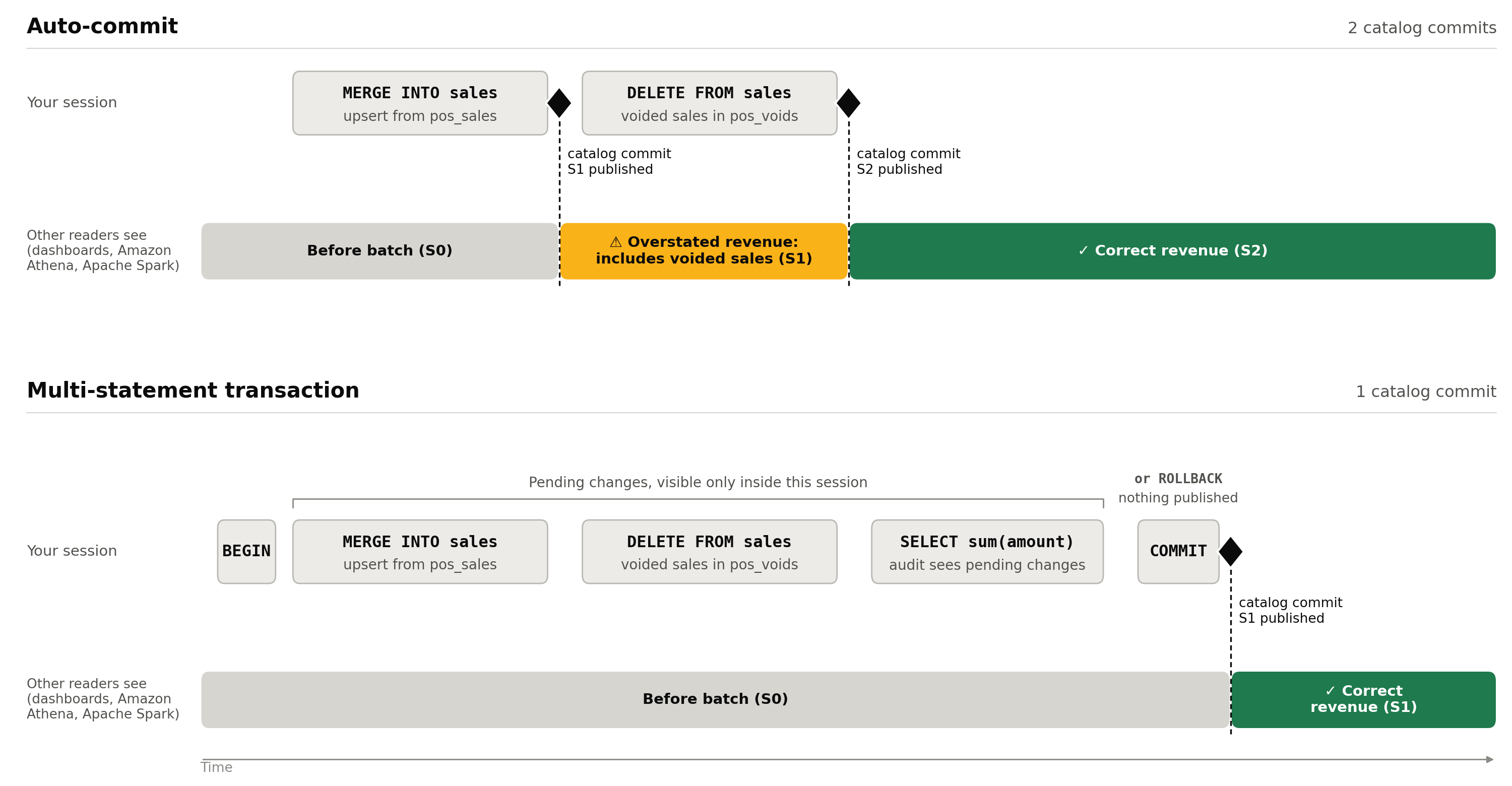
Timeline diagram comparing auto-commit with a multi-statement transaction. With auto-commit, MERGE and DELETE each make a catalog commit, so between the two commits other readers see overstated revenue that includes voided sales. In a multi-statement transaction, MERGE, DELETE, and the audit SELECT stay pending inside the session, and other readers see the table as it was before the batch until COMMIT publishes the correct revenue in one catalog commit. ROLLBACK publishes nothing.

Figure 1: What other readers see with auto-commit and with a multi-statement transaction

What you can run inside a transaction

Iceberg DML is accepted in an explicit transaction block, in a multi-statement command string, and in prepared statements, including those sent through the Amazon Redshift JDBC driver.

All writes in a transaction must go to the same Iceberg table. The table can be in the AWS Glue Data Catalog or Amazon S3 Tables, and you can reference it through an external schema or the auto-mounted awsdatacatalog catalog. Refer to the table by the same name throughout the transaction. Amazon Redshift identifies a table by how you reference it. If you reference one physical table through two external schemas, or through an external schema and awsdatacatalog, it counts as two tables. A write through the second name is rejected.

Statement inside the transaction Behavior
Reads of Iceberg, Redshift managed storage (RMS), and external tables, across databases Allowed
INSERT, UPDATE, DELETE, MERGE against one Iceberg table Allowed. Published as one snapshot at COMMIT
REFRESH MATERIALIZED VIEW on one Iceberg materialized view Allowed. The view is the transaction’s write target
Reads of the Iceberg table you are writing, by the same name Allowed. Sees your uncommitted changes
A write to a second Iceberg table Rejected
Any other write, before or after the Iceberg writes: RMS or temporary table DML, COPY, UNLOAD, GRANT, REVOKE, ANALYZE, or other data definition language (DDL) Rejected
DDL on an Iceberg table: CREATE TABLE, CREATE TABLE AS, ALTER TABLE, CREATE MATERIALIZED VIEW, DROP TABLE, DROP MATERIALIZED VIEW Rejected
An Iceberg write inside a stored procedure Rejected

A rejected statement fails and aborts the transaction, so nothing that ran before it is published.

The nightly job fits these rules: it reads the Iceberg tables pos_sales and pos_voids and writes only sales. If the job also clears processed rows from a staging table, do that after COMMIT. Inside the transaction, it would be a write to a second Iceberg table.

Note: This changes behavior for existing workloads. A single Iceberg DDL statement inside BEGIN … COMMIT used to succeed and is now rejected. Run Iceberg DDL as a standalone statement.

Cleaning up orphan files

Intermediate files written by a transaction that doesn’t commit aren’t referenced by any snapshot and become orphan files. For Amazon S3 Tables, unreferenced file removal is enabled by default for table buckets. For tables in the AWS Glue Data Catalog, enable the orphan file deletion table optimizer. It removes only files created after you enable it, so enable it before you start using multi-statement transactions.

Concurrent readers and writers

A multi-statement transaction gives you three guarantees:

  1. Atomic publishing: Other sessions and engines see none of your changes until COMMIT, and then see all of them in one snapshot.
  2. Read your own writes: Reads of the Iceberg table you are writing include your uncommitted changes, as long as you use the same name.
  3. Repeatable reads of each table: The first read of an Iceberg table fixes its version for the rest of the transaction. Later reads of that table return the same data, even if other sessions commit to it in the meantime.

Each table’s version is fixed at its first read, not when the transaction begins. An Iceberg table that you first read later in the transaction can include changes that other sessions committed after the transaction started. For example, suppose the nightly job reads sales and then looks up store details in an Iceberg stores table. The lookup includes changes that another session committed to stores in between:

-- Session 1                              -- Session 2
BEGIN;
SELECT * FROM iceberg_schema.sales;
-- fixes the version of sales
                                          INSERT INTO iceberg_schema.stores ...;
                                          -- auto-commit
SELECT * FROM iceberg_schema.stores;
-- first read of stores:
-- includes Session 2's insert
COMMIT;

RMS tables follow their own snapshot, taken at the transaction’s first statement and not coordinated with the Iceberg catalog.

Performance

To measure the performance impact, we compared committing each statement on its own against batching the same statements into multi-statement transactions. We report results relative to single-statement commits.

Setup: An Iceberg table registered in the AWS Glue Data Catalog in the US East (N. Virginia) Region (us-east-1), written from a single Amazon Redshift provisioned cluster. Throughput tests run one session per writer over a fixed window. Each writer runs its transactions back to back. A transaction whose commit fails is rolled back and not counted. Results vary with statement size, partitioning, and contention.

Latency

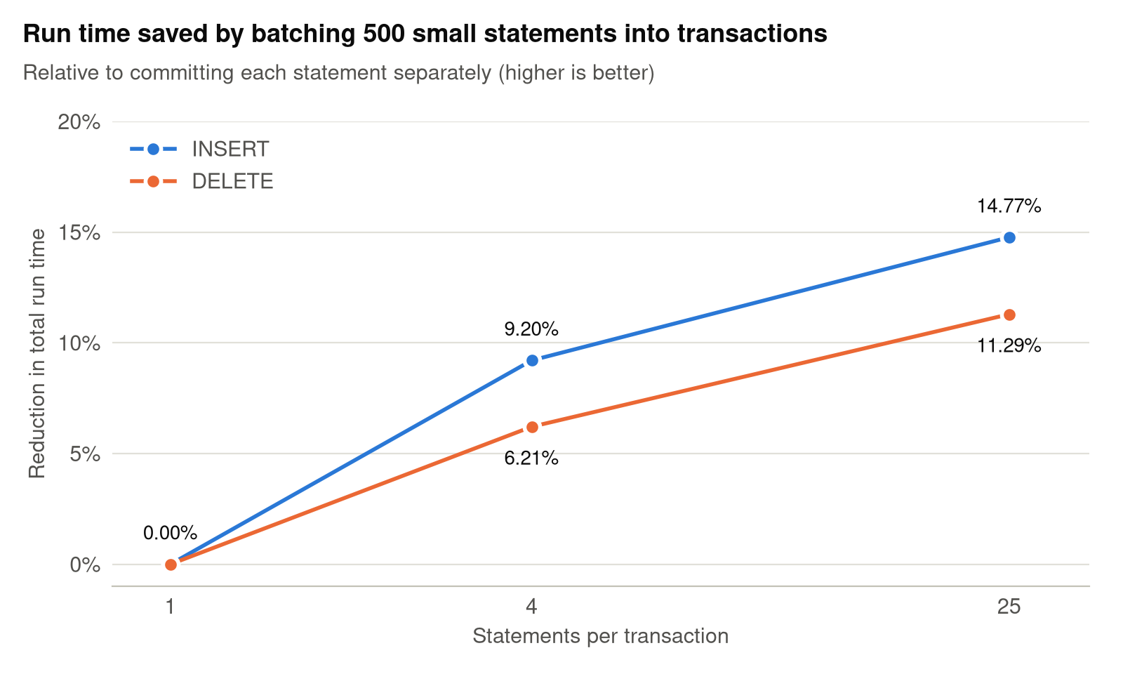
We first measured the case that batching is meant to help: many small statements, where commits rather than data movement dominate the run time. Each configuration runs the same 500 small statements against one table, and only the number of statements per commit changes.

Line chart of the reduction in total run time from batching 500 small statements, by statements per transaction (1, 4, and 25), compared to committing each one separately. INSERT: 0.00%, 9.20%, and 14.77%. DELETE: 0.00%, 6.21%, and 11.29%.

Figure 2: Reduction in total run time for 500 small statements, relative to committing each statement separately

As Figure 2 shows, batching 25 statements per commit reduced total run time by 14.77% for INSERT and 11.29% for DELETE, compared to committing each statement separately. More than half of that gain already arrives at 4 statements per commit (9.20% and 6.21%). The gain comes from paying one catalog commit per transaction instead of one per statement, and from less per-statement transaction overhead.

However, when each statement already does heavy data work, the time saved by combining commits is too small to notice. Batching statements into one transaction doesn’t make the job meaningfully faster.

Throughput

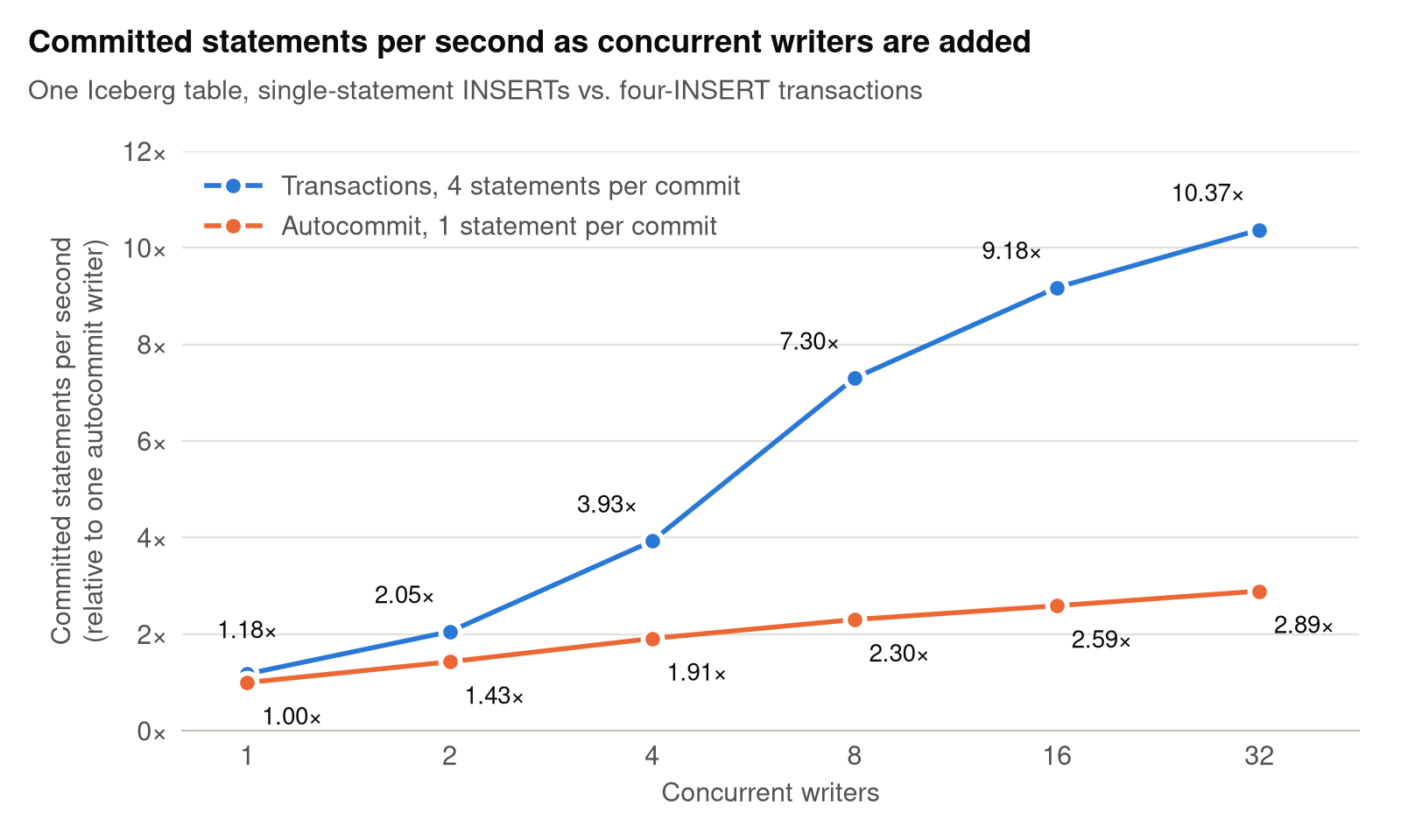
With multi-statement transactions, a single catalog commit can carry the changes from several statements, which raises write throughput. To measure this, we ran an increasing number of concurrent writers against one table, comparing auto-commit single-statement INSERTs with transactions of four INSERTs. Figure 3 shows committed statements per second, normalized to a single auto-commit writer.

These results were measured with conflict resolution, which applies to every multi-statement transaction. Another writer can commit to the same table while your transaction is open. If the two sets of changes don’t overlap, Amazon Redshift rebases your transaction onto the latest table version and commits it as one snapshot, without re-running any of its statements. Only a genuine conflict, where both writes changed the same data, fails the COMMIT. In that case, retry the transaction from your application.

Line chart of committed statements per second for 1 to 32 concurrent writers, normalized to one auto-commit writer. Transactions of four INSERTs rise from 1.18x to 10.37x. Auto-commit single-statement INSERTs rise from 1.00x to 2.89x.

Figure 3: Committed statements per second as concurrent writers are added, normalized to a single auto-commit writer

The advantage grows with concurrency. With one writer, transactions commit 1.18× as many statements as auto-commit. As writers are added, the number of catalog commits per second levels off for both configurations, but each transaction commit carries four statements instead of one. At 32 concurrent writers, auto-commit reaches 2.89× the single-writer rate and transactions reach 10.37×. That is 3.59 times as many committed statements in the same window.

Conclusion

Multi-step writes are the normal shape of a data pipeline. Until now, each step against an Iceberg table was visible on its own and you could undo it only by hand. With multi-statement transactions, Amazon Redshift publishes a group of DML statements against one Iceberg table as a single atomic snapshot. Readers never see a half-applied change, and a failure leaves nothing to undo. The pipeline also pays one catalog commit instead of one per statement. To get started, upgrade to Patch 206 or later.

To learn more about Iceberg support in Amazon Redshift, see the following resources:


About the authors

Shiyu Xu

Shiyu Xu

Shiyu is a software engineer at Amazon Redshift who builds core storage infrastructure, including transactional support for Apache Iceberg tables, backup, and the data storage layer.

Jiuzhi Yu

Jiuzhi Yu

Jiuzhi is a software engineer at Amazon Redshift working on transactional support for Apache Iceberg tables, backup, and the data storage layer.

Xiening Dai

Xiening Dai

Xiening is a principal software engineer leading various efforts in Amazon Redshift query execution and data lake processing.

Madhukiran Vaddi

Madhukiran Vaddi

Madhukiran is an engineering lead with the Amazon Redshift team. Leads Iceberg transaction support, including conflict resolution and multi-table transactions, and Redshift concurrency scaling, backups, and durability. Madhukiran is passionate about building reliable data infrastructure at cloud scale.

Srishti Mittal

Srishti Mittal

Srishti is a Product Manager at AWS, with a focus on making open data lakes performant and interoperable across analytics engines. She leads product strategy for open table formats such as Apache Iceberg, partnering with customers and field teams to turn real-world data lake challenges into product capabilities.

Adapting to AI penetration testing orchestrators: The Modern Security Model

Post Syndicated from Blake Darché original https://blog.cloudflare.com/adapting-to-ai-penetration-testing-orchestrators/

Over the last month, the number of Large Language Model (LLM) penetration testing and orchestration frameworks has exploded. Just a few weeks ago, ARTEX — an open source agentic penetration testing system that automates offensive security workflows — was the only framework available. In just the last three days, we have seen over 50 framework families attempt to scan Cloudflare customers globally. The number of Internet Protocol (IP) addresses seen running these frameworks has grown into the thousands and continues to increase daily. The proliferation of these frameworks has significantly changed the status quo in cyber defense: defenders are struggling to keep up with the volumetric nature of these autonomously guided attacks.

ARTEX was taken down by its creator Autumn-27 on October 8. (“The malicious exploitation of this tool runs entirely counter to its original intent,” they wrote in Chinese.) But in the month since, the ecosystem has exploded with new fragmented versions of it. There are now over 12,000 repositories, with several hundred unique forks containing lineage from the original repository. Additionally, hundreds of other similar agentic orchestration frameworks have been created since October 8. Daily requests of AI penetration testing (pentesting) and exploitation tools has grown by 30x since October 1. These tools have also begun chaining stolen customer credentials in some of the more complex attacks, such as lateral movement chaining throughout an environment.

We expect these frameworks to continue to proliferate, and every organization should be prepared to address this threat. To counter LLM-based pentest frameworks, we recommend that all organizations adopt what we call the Modern Security Model, which has six key pillars:

  • Fortify the front gate: Implement a Web Application Firewall (WAF) with advanced rules such as rate limits.
  • Security station in the foyer: Anomaly detection on all web applications your customers access.
  • Identify phony visitors: Implement Bot Defense.
  • Remove the back door: Implement Identity-Gated Access for all high-risk external and internal web applications.
  • Inspect deliveries: Enforce validated schemas and explicit security controls.
  • Neighborhood watch: Implement Threat Intelligence to gain visibility into attacks.

What is an LLM penetration and exploitation orchestrator?

Open-source pentesting frameworks are able to orchestrate AI agents to carry out stages of the traditional Cyber Kill Chain at scale. Tools like ARTEX have the ability to quickly plug in existing Model Context Protocol (MCP) and connect traditional standalone pentesting tools in novel ways. Some even allow operator direction on what type of task to accomplish. These tools can map and enumerate environments, both from the inside and outside. ARTEX and its forks map assets and environments onto a graph, allowing multiple independent parallel agents to enumerate, verify, prototype, and attack at the speed of inference. These tools turn compromises into a hill-climbable problem, which agents are specifically good at.

The AI LLM pentesting tools that currently exist

We are currently tracking 50+ AI LLM agents. The table below shows the top five LLM penetration and exploitation orchestrators. Each is extremely popular (1k+ GitHub stars) and fully autonomous. The fully autonomous nature of these agents represents a doctrinal shift in offensive cyber capabilities:

  • Human skills are no longer the limit: A harness performs every step of the OODA loop by observing the environment, orienting itself to prioritize valuable and/or vulnerable targets, decide on an action, and act autonomously.
  • Speed increase: Having multiple parallel agents working towards a goal is a large shift compared to single operator or multiple operator augmented by AI.
  • Scale: A single operator can target multiple organizations at the same time, greatly increasing their blast radius.
  • Small mistakes are easily discovered: Autonomous frameworks relentlessly and systematically test exposed services, including their configurations.

Architecture

Planning model

Built-in capabilities/execution environment

Post-exploitation capabilities

ARTEX (and forks)

Planner and parallel agents

Graph of goals, leads, and findings is linked to separate asset graph of target

Directly on host or container with network/root access, can install/develop tools as needed

Nothing built-in, requires user instruction

LuaN1aoAgent

Supervisor agent, planner agent, and generic executor agents

Three graphs, with goals/tasks/blockers, evidence/hypothesises/exploits, and target/local

Container with network/user access, can develop tools as needed and install user packages

Built-in SSH and Chisel for tunneling and attempted reconnection after disruption

Decepticon

Orchestrator agent dispatching specialist sub-agents

Graph of objectives with prerequisites

Kali container running as root, can develop tools as needed

Dedicated post-access, Active Directory and cloud pivoting skills

Cairn

Dispatcher orchestrating work to existing AI harnesses (Codex, Claude Code, Pi)

Graph of facts and leads; new nodes trigger dispatcher

Kali container with root access or directly on host, can develop tools as needed

Prompt guidance and Kali tools

PentestGPT-Agent

Supervisor agent and one generic executor agent

Task list with dependencies, goals, and evidence

Run on host, can develop tools as needed

Nothing built-in, requires user instruction

Observations from the world's largest network

As of November 12, ARTEX and its forks make up over 60% of currently known AI penetration testing orchestrators. The charts below help us understand how adoption of these tools has changed over the past six weeks. Since the removal of the original ARTEX repository on October 8, traffic has grown more than tenfold, and has increased more than 30x since October 1.

As demonstrated above, the takedown of ARTEX on October 8 (and widespread reporting of it) likely caused a hydra effect, where the removal of the original repository led to a massive increase in the number of forks and modifications which can be seen in the steep acceleration of unique instances around October 8.

Identity-chained LLM exploitation

Over the last eight weeks, our Cloudforce One team has been called into multiple incident response investigations involving ARTEX and ARTEX-derived LLM exploitation frameworks. We’ve seen firsthand how exposed credentials are being chained with LLM-based exploitation frameworks to gain the upper hand over defenders.
We observed multiple incidents in which a threat actor gained initial access to a hyperscaler environment and pivoted directly into the customer's Cloudflare environment. Root-cause analysis revealed a common credential hygiene failure. Attackers repeatedly compromised static, non-expiring tokens running inside CI/CD pipelines, which granted broad, cross-environment access across the organization's hyperscaler infrastructure. LLM frameworks greatly expand the likelihood of a client’s API key being laterally leveraged to take over other tenant environments.

ARTEX in action

As part of one incident response investigation, our team observed ARTEX gaining access to a compromised account-level API token previously used for CI/CD with no IP restrictions or rate limiting. Available evidence indicated that the compromise most likely originated through a third-party hyperscaler.

We observed that a large number of new Worker scripts had been created with distinct names such as artex-*, artex-pgrecon-*, artex-pgw-*, and artex-do-*. The naming of each Worker script correlated to distinct behaviors and actions it was taking, and was often postfixed by an alphanumeric identifier. We observed activity in excess of 69 requests per minute across multiple unique parts of their Cloudflare infrastructure and 400 database dump requests in an hour. We also observed attempted persistence mechanisms and attempts to validate session tokens for other third-party applications. While we believe that much of this activity was lightly guided by the human operator, this is just one example of the speed and breadth that ARTEX and similar frameworks can achieve post-compromise.

Our recommendation: the Modern Security Model

Large Language Models increase the ability of a threat actor to rapidly iterate through the Cyber Kill Chain against a target. They do this by giving the actor the advantage of speed and validation. Each step of the Cyber Kill Chain can be validated and fed into the next stage of the attack. This level of orchestration is unparalleled and effectively vaporizes legacy cyber security models. A modern model must be used against these attacks.

To help explain this model further, let’s use the metaphor of protecting a house on an estate. Each section below outlines how to defend against the threat at each step.

Fortify the front gate: implement traffic control and a WAF with advanced rules

Before anyone even sets foot on your lawn, they have to reach the perimeter fence.

On an unprotected estate, an adversary can drive an endless fleet of decoy trucks straight into your driveway, completely blocking the entrance and smashing through the barriers (Layer 3/4 volumetric floods and direct IP probing).

With perimeter gate security in place, all incoming traffic is routed through massive, distributed outer gates miles away from the main house. Rogue delivery trucks are filtered out to the highway, rogue utility tunnels trying to wiretap your property are severed, and only legitimate foot traffic ever reaches your home address.

Network traffic control serves as an important role in stopping volumetric attacks.

A security station in the foyer: anomaly detection

Once visitors arrive at the main entry, they meet a strict security station at the foyer.

Automated prowlers don't just kick the door; they disguise themselves. They attempt weird ways to get in the door — stuffing paper into the lock, trying variations like //front-door//back-room/ to trick the mechanism into swinging open.

The security guard at the door enforces clear rules:

  • You cannot knock 500 times in five seconds.
  • You cannot disguise your path with trickery.
  • You cannot attempt to roll a massive flatbed cart through the front hall to haul away the house's internal blueprints (diagnostic heap dumps). Suspicious behavior is turned away immediately.
  • Implement security keys and hardware based FIDO keys.

Web Application Firewall (WAF) serves as a key defense mechanism in stopping application exploitation through rate limits and anomaly detection.

Identify phony visitors: implement Bot Defense

A sophisticated intruder rarely looks like a masked burglar; they disguise themselves as ordinary visitors. But automated agents, headless browser scrapers, and AI reconnaissance tools don't act like real people.

They don't blink, their posture is unnervingly rigid, their cadence is mechanical, and their "identification" is often a sloppy imitation of a real visitor badge.

Bot Defense and challenges act as behavioral specialists watching the crowd through one-way glass. It flags the unnatural cadence, catches the synthetic micro-behaviors, and quietly escorts the machines off the property before they can touch a single doorknob.

Remove the back door: implement Identity-Gated Access and micro-segmentation

Many homes historically were built with side doors or a cellar hatch (internal admin panels, /actuator diagnostic endpoints, and remote gateways). Even if locked, a prowler could stand on the sidewalk, shine a flashlight on the cellar door, and start picking the lock.

Zero Trust application access does something radical: it bricks up the doorway from the outside and restricts which rooms can be entered.

To anyone wandering the perimeter, the cellar door does not exist. There is no lock to pick, no handle to rattle, and no light on inside. The only way in is with an escort who checks your biometric badge, confirms your device has a clean bill of health, and steps you directly into the specific room you need — leaving the rest of the house out of view.

For those who do enter, you have to ensure they cannot breach rooms next to the room they enter. Micro-segmentation is a highly effective strategy at stopping lateral movement. It limits compromised credentials from breaching production, test, and development systems.

Inspect deliveries: enforce validated schemas and explicit security controls

You receive daily supply deliveries to your estate — groceries, mail, maintenance parts. In digital terms, this is your incoming API traffic, which must be inspected and verified.

Intruders often attempt to bypass controls by sending unvalidated payloads or forged delivery manifests meant for restricted internal systems.

The porch protocol mandates thorough inspection and schema validation for all traffic:

  • Every incoming request must undergo OpenAPI schema validation to ensure it strictly conforms to expected definitions and structures.
  • Drivers and couriers must present validated mutual TLS (mTLS) certificates to establish trusted, authenticated connections.
  • Any request failing inspection or missing valid credentials is rejected immediately at the boundary.
  • Default-Deny Posture: Every positive security implementation ends with an explicit deny-all rule at the bottom of the ruleset.

Neighborhood watch: implement threat intelligence to gain visibility into attacks

Even with ironclad walls, an isolated property can be vulnerable if a syndicate invents a brand-new infiltration technique across town.

Threat intelligence acts as your warning network with neighboring estates. When a rogue actor sets up a new command-and-control safehouse down the road or begins deploying dynamic tunneling vans in your district, you receive an early dossier. Your estate updates its watchlists, recalibrates its sensors, and slams the gate shut before the actor ever turns onto your street.

How to get real-time help

ARTEX and similar LLM-based frameworks pose a significant challenge to legacy cyber defense models. Even the historical defense-in-depth model — which emphasizes a classic network DMZ — falls short in today's complex architectures. Tomorrow's attacks will only advance as orchestration tools become the new normal.

Securing legacy equipment and on-premises devices requires an identity-gated approach that logically makes these devices impossible to reach on the Internet. Beyond identity, slowing or making lateral movement more noisy is the goal of micro-segmentation. This architecture emphasizes a containment-first approach to security, which is essential when users are consistently losing their keys. When combined, the elements of the Modern Security Model are the answer to this vexing problem.

If you are facing an active security incident and need the Cloudforce One team on the ground to help respond to the incident or require threat intelligence support, please contact us immediately. If you need help implementing the Modern Security Model outlined here, please contact our Solutions Engineering team.

Build a self-healing ETL pipeline with Amazon Bedrock AgentCore

Post Syndicated from Kevin Tinn original https://aws.amazon.com/blogs/big-data/build-a-self-healing-etl-pipeline-with-amazon-bedrock-agentcore/

Extract, transform, and load (ETL) pipelines break silently. Schema drift, missing fields, and type mismatches corrupt downstream analytics. The typical fix is manual: detect the error, triage it, patch the record, update the code, redeploy. As data volumes grow, this detect-triage-fix-deploy cycle doesn’t scale. A self-healing pipeline built on Amazon Bedrock AgentCore, a platform to build, connect, and optimize agents at scale with any framework or model, can repair itself.

The self-healing pipeline in this post fixes its own data, persists the corrections, and can propose pull requests to help prevent the same errors from recurring (optional, requires repository credentials).

In this post, you will build a self-healing ETL pipeline that uses AWS Glue and Amazon Bedrock AgentCore. The pipeline automatically corrects bad records using domain knowledge and writes them back to the data lake. When you configure the optional repository integration, it also generates code reviews with recommended fixes. The result is a closed loop on data quality that reduces the need for human intervention. You’ll cover the architecture, deploy the infrastructure with the AWS Cloud Development Kit (AWS CDK), and test the data correction workflow with sample data, including a before-and-after record comparison.

Amazon Bedrock Knowledge Bases with pre-computed correction strategies stored in Amazon S3 Vectors, a capability of Amazon Simple Storage Service (Amazon S3), reduce the time to create and deploy corrective measures. A manual workflow involves an engineer diagnosing the error pattern, writing a fix, and deploying it through a release cycle. This system applies known corrections within seconds of detection. It also surfaces new patterns to the team with full context, including a proposed code fix. When records fail validation, automatic correction keeps them flowing to consumers instead of sitting in a dead-letter queue awaiting manual triage. Confidence threshold and human-notification fallback provide built-in oversight governing this autonomous agentic behavior. For additional responsible AI controls, consider Amazon Bedrock Guardrails, grounding, and content filtering.

The problem: Data quality at scale

Consider a hypothetical weather data system ingesting National Oceanic and Atmospheric Administration (NOAA) records across 15 schema types: temperature, precipitation, wind, pressure, humidity, visibility, cloud cover, solar radiation, and more. In a system like this, sensor failures, schema drift, and producer bugs can cause a meaningful percentage of records to fail validation.

Today, that means:

  • Engineers get paged about bad data hours after it arrives.
  • Someone manually inspects the error, determines the fix, and patches the record.
  • A developer traces the root cause back to upstream code and submits a fix.
  • The pipeline is redeployed, until the next variant of the same error appears.

Each step requires a person, a tool, and a context switch. A self-healing pipeline captures that correction knowledge and applies it automatically the next time a similar error appears.

Prerequisites

To implement this pattern, you need:

  • An AWS account with permissions to create resources in the following services:
    • Amazon S3 (including Amazon S3 Vectors), AWS Glue, Amazon Bedrock.
    • Amazon Elastic Container Registry (Amazon ECR), AWS CodeBuild, AWS Lambda.
    • Amazon Simple Notification Service (Amazon SNS), AWS Secrets Manager, AWS Identity and Access Management (IAM).
  • Amazon Bedrock model access enabled for Anthropic Claude (agent reasoning) and Amazon Titan Embeddings V2 (knowledge base indexing) in your target AWS Region. For model availability by Region, refer to supported models by AWS Region in Amazon Bedrock (https://docs.aws.amazon.com/bedrock/latest/userguide/models-regions.html).
  • AWS CDK CLI installed (npm install -g aws-cdk@latest) with Python 3.10+.
  • Finch or Docker for building agent container images (CDK builds ARM64 images through CodeBuild, but local testing requires a container runtime).
  • Familiarity with Amazon S3 data lake patterns and basic understanding of multi-agent orchestration concepts.

The sample implementation uses the Strands Agents SDK for agent development and AWS CDK (Python) for infrastructure. Deploy all resources within a single AWS Region.

Solution overview

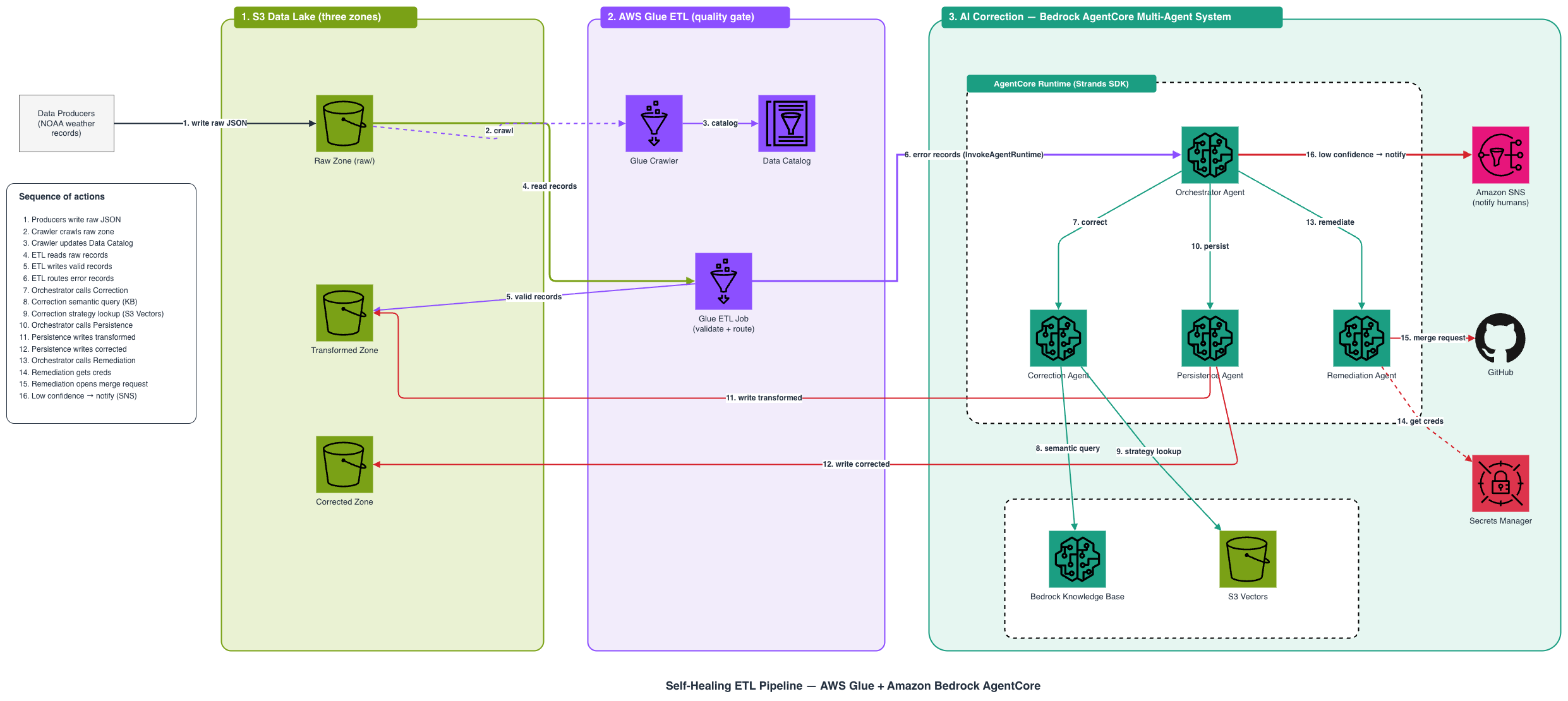
This solution replaces that manual cycle with a multi-agent system that automates three things: correct the data, persist the fix, and remediate the code. The following diagram shows the complete architecture:

Architecture diagram showing the full end-to-end pipeline flow: data producers upload to the S3 raw zone, AWS Glue validates and transforms records, error records route to the Bedrock AgentCore multi-agent system for correction, persistence, and remediation, with SNS notifications for manual intervention

Figure 1: End-to-end architecture of the self-healing ETL pipeline

Here’s how data flows through the pipeline:

  1. Ingest – Data producers write weather records directly to an Amazon S3 raw landing bucket, organized by schema type under the raw/ prefix. Records are preserved unmodified.
  2. Transform – An AWS Glue ETL job validates each record against its declared weather schema and writes valid records to the transformed zone. Records that fail validation are classified by error type (missing field, type mismatch, schema violation, invalid format) and routed to the AgentCore system.
  3. AI correction – A four-agent system on Bedrock AgentCore handles the error:
    • Orchestrator agent coordinates the sequential workflow: correction to persistence to remediation.
    • Data correction agent queries domain knowledge to find and apply a high-confidence fix.
    • Data persistence agent writes the corrected record back to the data lake.
    • Code remediation agent identifies the root cause and proposes a pull request to help prevent recurrence.
  4. Notify – When no high-confidence correction is found, the orchestrator publishes a notification through Amazon Simple Notification Service (Amazon SNS) for manual intervention rather than applying a bad fix.

How validation and error routing work

The AWS Glue ETL job acts as the quality gate. It validates each record against a dispatcher that maps each of the 15 schema types to a dedicated validator. Each validator checks required fields, data types, enum values, and numeric constraints:

def validate_record(record: dict) -> dict:
    """Validate a single weather record against its declared schema_type."""
    schema_type = record.get("schema_type")
    if schema_type not in VALID_SCHEMA_TYPES:
        return {"valid": False, "error_type": "invalid_format",
                "error_details": f"Unknown schema_type: '{schema_type}'"}

    data = record.get("data")
    validator = SCHEMA_VALIDATORS.get(schema_type)
    error_details = validator(data)

    if error_details:
        # Validators emit only three message shapes, so once missing-field and
        # type-mismatch are ruled out, the else is always a constraint/enum/range failure
        if "Missing required field" in error_details:
            error_type = "missing_field"
        elif "Type mismatch" in error_details:
            error_type = "type_mismatch"
        else:
            error_type = "schema_violation"
        return {"valid": False, "error_type": error_type,
                "error_details": error_details}

    return {"valid": True, "error_type": None, "error_details": None}

When a record fails, the job packages it as an error record, preserving the original payload, the classified error type, and the validation details. It then routes the error to the AgentCore orchestrator through the InvokeAgentRuntime API. This is the handoff point where the pipeline stops being a passive data mover and becomes an active self-healing system.

Multi-agent orchestration with Bedrock AgentCore

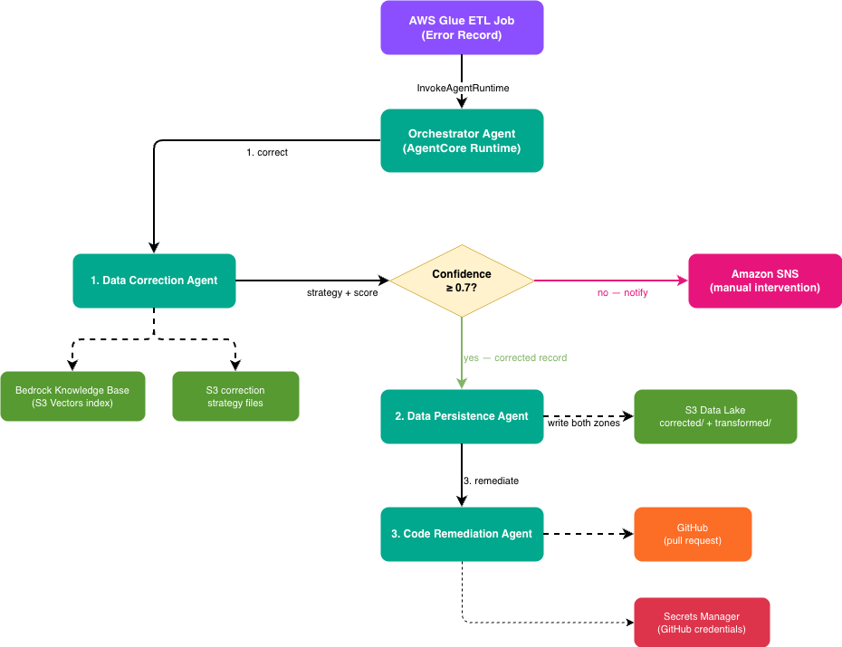
The orchestrator agent coordinates the entire correction workflow. It receives an error record from the AWS Glue ETL job and drives a sequential path through the specialized agents, degrading gracefully to a human notification when it can’t correct with confidence of at least 70 percent. If a step fails, it stops rather than propagating bad data downstream. The following diagram shows that flow and how each agent connects to its knowledge sources and outputs:

AgentCore multi-agent workflow: the orchestrator receives error records from Glue, invokes the correction agent (backed by the Knowledge Base and S3 correction files), checks the confidence threshold, then routes to the persistence agent (writing both data lake zones) and remediation agent (submitting repository pull requests), or to SNS when confidence is too low

Figure 2: Multi-agent orchestration workflow on Amazon Bedrock AgentCore

The diagram shows the orchestrator receiving an error record from AWS Glue and invoking the correction agent, which draws on the Amazon Bedrock knowledge base and the S3 correction files. The orchestrator then checks the correction’s confidence against the threshold: if it clears, the orchestrator routes the record to the persistence agent (which writes to both data lake zones) and the remediation agent (which opens a repository pull request). If it falls short, the orchestrator sends the record to Amazon SNS for manual review.

Each agent is a containerized application built with the Strands Agents SDK and deployed as an AgentCore runtime, a capability of Amazon Bedrock AgentCore.

The orchestrator doesn’t contain correction logic itself. It delegates to specialized agents and makes routing decisions based on their responses. This separation means you can update correction strategies without touching orchestration logic. You can also swap in a different persistence backend without affecting the correction agent.

Two-source correction: Breadth meets precision

The correction agent’s job is to find the right fix with high confidence. It uses two complementary knowledge sources:

Amazon Bedrock Knowledge Bases. The agent sends a natural language query describing the error to a knowledge base backed by Amazon S3 Vectors and Amazon Titan Embeddings V2. Amazon Bedrock Knowledge Bases provides fully managed Retrieval Augmented Generation (RAG) capabilities. In this case the knowledge base provides semantic search over indexed domain documents (NOAA data guides, schema definitions, error pattern catalogs) and returns ranked results with relevance scores.

def _query_knowledge_base(error_record: dict) -> dict:
    """Query Amazon Bedrock KnowledgeBase for correction strategies."""
    query_text = (
        f"How to correct a {error_record.get('error_type')} error "
        f"in a {error_record.get('schema_type')} weather record? "
        f"Error details: {error_record.get('error_details')}"
    )
    response = bedrock_agent_runtime.retrieve(
        knowledgeBaseId=KNOWLEDGE_BASE_ID,
        retrievalQuery={"text": query_text},
        retrievalConfiguration={"vectorSearchConfiguration": {"numberOfResults": 3}},
    )

    results = response.get("retrievalResults", [])
    top_result = results[0]
    score = top_result.get("score", 0.0)
    content = top_result.get("content", {}).get("text", "")
    source = top_result.get("location", {}).get("s3Location", {}).get("uri", "unknown")
    return {"strategy": content, "score": score}

Amazon S3 Vectors. In parallel, the agent does a direct lookup for a pre-computed correction strategy at correction/{schema_type}/{error_type}.json. These files contain specific fix instructions with confidence scores for known error combinations:

{
  "correction_strategy": "For missing temperature fields, check if the complementary unit field is present (celsius/fahrenheit) and compute the missing value using the conversion formula.",
  "confidence": 0.85
}

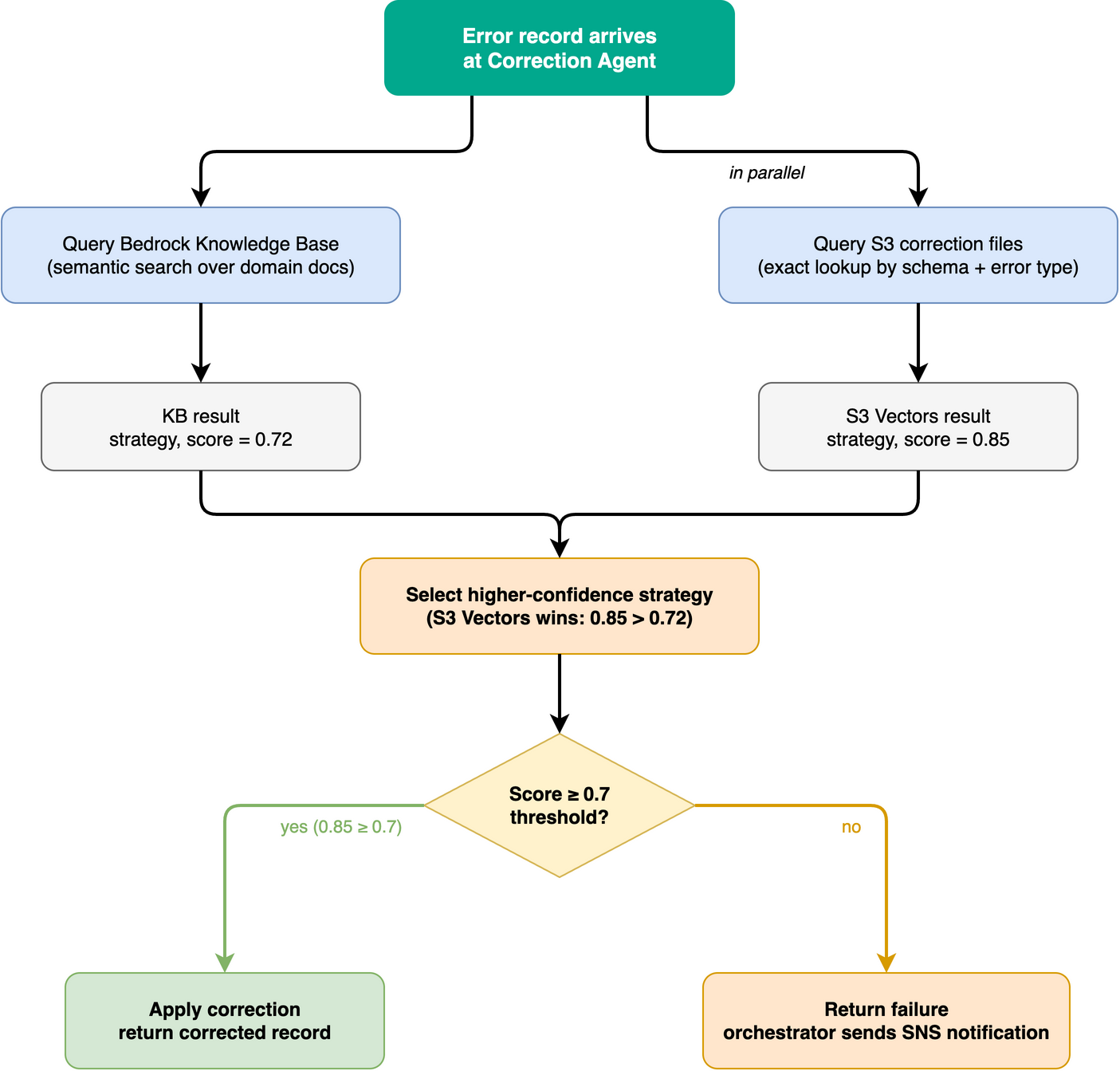
The agent compares both results and picks whichever has the higher confidence score. If the selected strategy meets the threshold (default 0.7), the correction is applied. If not, the orchestrator sends an SNS notification for manual intervention.

This design gives you:

  • Breadth – The knowledge base can reason about novel error patterns using domain knowledge from indexed documents, even for combinations it hasn’t seen before.
  • Precision – S3 Vectors provide instant, high-confidence fixes for known combinations without requiring Amazon Bedrock model inference.
  • Graceful degradation – If neither source returns a confident answer, the system notifies humans rather than applying a bad fix.

The correction agent decides which fix to apply by weighing two knowledge sources against a confidence threshold. The following flowchart shows that decision logic, with example confidence scores:

Two-source correction decision flow: the correction agent queries the Knowledge Base and S3 correction files in parallel, selects the higher-confidence strategy, applies the correction if the score meets the 0.7 threshold, or returns failure triggering an SNS notification

Figure 3: Two-source correction decision flow with a confidence threshold

The flowchart shows the correction agent querying the Amazon Bedrock knowledge base and the S3 correction files in parallel, then selecting the higher-confidence strategy (for example, an S3 score of 0.85 over a knowledge base score of 0.78). If the selected score meets the 0.7 threshold, the agent applies the correction and returns the corrected record. If it falls short, the agent returns a failure. This triggers an Amazon SNS notification for manual review.

Closing the loop: Automated code remediation

Most data quality systems stop at fixing the record. This pipeline goes further: the remediation agent traces the error back to its source and proposes a code fix.

After a successful correction, the orchestrator invokes the code remediation agent, which:

  1. Reads the source repository – Connects to the repository using credentials stored in AWS Secrets Manager.
  2. Analyzes root cause – Correlates the error type, schema type, and correction applied to identify which upstream code produced the bad data.
  3. Generates a code change – Produces recommended changes that preserve existing logic (it does not recommend disabling validation or removing functionality).
  4. Submits a pull request – Uses GitHub MCP Server to create a branch, commits the changes, and opens a pull request with the root cause analysis in the description.
def _create_mcp_client(auth_token: str):
    return MCPClient(
        lambda: streamable_http_client(
            GIT_MCP_URL,
            http_client=create_mcp_http_client(headers=headers),
        ),
        startup_timeout=GIT_MCP_TIMEOUT,
    )

This means recurring errors get fixed at the source rather than only patched in the data lake. Over time, the pipeline’s error rate decreases as upstream code improves.

The data lake: Three zones, one truth

The S3 data lake uses prefix-based organization across three zones. Downstream consumers see complete data for processed records, whether a record was valid on first pass or corrected by the agents:

Zone Purpose Written By
raw/ Unmodified original records (audit trail) Data producers
transformed/ Validated, schema-conformant records Glue ETL Job + Persistence Agent
corrected/ Corrected records with correction metadata Persistence Agent

The persistence agent writes corrected records to both zones. The corrected zone provides auditability, capturing what was wrong and how it was fixed. The transformed zone gives downstream consumers a complete dataset without needing to union multiple paths.

Deploy the pipeline

With the architecture understood, deploy the pipeline. The complete sample implementation is available in the GitHub repository. The entire system is defined in AWS CDK (Python). A single cdk deploy command provisions all infrastructure, builds container images through CodeBuild, creates the knowledge base, and sets up the AgentCore runtime resources.

Step 1: Clone the repository and install dependencies

git clone https://github.com/aws-samples/sample-self-healing-etl-pipeline.git
cd sample-self-healing-etl-pipeline

python3 -m venv .venv
source .venv/bin/activate
pip install -r requirements.txt

Step 2: Bootstrap CDK and deploy infrastructure

Deploy all stacks with a single command. CDK handles dependency ordering, container image builds, knowledge base creation, and runtime provisioning automatically:

# Bootstrap CDK (first time only)
cdk bootstrap aws://$(aws sts get-caller-identity --query Account --output text)/us-east-1

# Deploy all stacks
cdk deploy --all \
  --require-approval broadening \
  -c aws_region=us-east-1 \
  -c aws_account=$(aws sts get-caller-identity --query Account --output text) \
  -c [email protected] \
  -c git_repo_url=https://github.com/aws-samples/sample-self-healing-etl-pipeline

CDK deploys the following stacks in dependency order:

Stack Resources
WeatherDataLakeStack S3 output bucket (transformed + corrected zones)
WeatherIngestionStack S3 raw landing bucket
WeatherGlueStack Crawler, Data Catalog, ETL job, automatic script upload
WeatherKnowledgeBaseStack S3 Vector bucket + index, Amazon Bedrock Knowledge Base + Data Source, automatic document upload + ingestion, agent vector buckets with generated lookup files
WeatherAgentCoreStack ECR repos, IAM roles, SNS topic, Secrets Manager, CodeBuild projects with automatic ARM64 image builds
WeatherAgentCoreRuntimeStack Four AgentCore Runtime resources

To pass repository credentials for the optional remediation step:

./scripts/set_git_token.sh --token <your_github_token>

The stacks pass resources to each other through constructor arguments in app.py. For example, the AgentCore runtime stack receives the IAM roles and ECR repository URIs from the AgentCore stack. It also receives the knowledge base ID from the knowledge base stack:

# app.py: cross-stack wiring
agentcore_stack = AgentCoreStack(
    app,
    "WeatherAgentCoreStack",
    notification_email=config["notification_email"],
    git_repo_url=config["git_repo_url"],
    knowledge_base_id=knowledge_base_stack.knowledge_base.attr_knowledge_base_id,
    correction_vectors_bucket=knowledge_base_stack.correction_vectors_bucket.bucket_name,
    persistence_vectors_bucket=knowledge_base_stack.persistence_vectors_bucket.bucket_name,
    corrected_bucket=data_lake_stack.output_bucket.bucket_name,
    transformed_bucket=data_lake_stack.output_bucket.bucket_name,
    log_retention_days=config["log_retention_days"],
    env=env,
)

# Runtime stack deploys last, after CodeBuild pushes the agent images to ECR
runtime_stack = AgentCoreRuntimeStack(
    app,
    "WeatherAgentCoreRuntimeStack",
    agent_roles=agentcore_stack.agent_roles,
    ecr_repo_uris={name: repo.repository_uri for name, repo in agentcore_stack.ecr_repos.items()},
    notification_topic_arn=agentcore_stack.notification_topic.topic_arn,
    git_secret_arn=agentcore_stack.git_secret.ref,
    knowledge_base_id=knowledge_base_stack.knowledge_base.attr_knowledge_base_id,
    correction_vectors_bucket=knowledge_base_stack.correction_vectors_bucket.bucket_name,
    persistence_vectors_bucket=knowledge_base_stack.persistence_vectors_bucket.bucket_name,
    corrected_bucket=data_lake_stack.output_bucket.bucket_name,
    transformed_bucket=data_lake_stack.output_bucket.bucket_name,
    env=env,
)

One wiring detail deserves mention: the AWS Glue stack deploys before the runtime stack exists. This means the orchestrator ARN can’t be passed as a CDK reference without creating a circular dependency. Instead, the runtime stack writes the ARN to an AWS Systems Manager (SSM) parameter (/weather-etl/orchestrator-runtime-arn) and the AWS Glue job reads it at job runtime.

Step 3: Verify knowledge sources

The knowledge sources populate automatically during cdk deploy. Domain documents (schema definitions, error patterns, NOAA data guides) upload from the repository’s knowledge_base/ folder to the knowledge base source bucket. A custom resource then triggers the knowledge base ingestion job. Correction strategy files and storage mappings are generated from the same documents and uploaded to the agent vector buckets.

Verify the population completed:

# Resolve the auto-generated vector bucket names from stack outputs (run once)
CORRECTION_BUCKET=$(aws cloudformation describe-stacks \
  --stack-name WeatherKnowledgeBaseStack \
  --query "Stacks[0].Outputs[?ExportName=='WeatherKB-CorrectionVectorsBucketName'].OutputValue" \
  --output text)

PERSISTENCE_BUCKET=$(aws cloudformation describe-stacks \
  --stack-name WeatherKnowledgeBaseStack \
  --query "Stacks[0].Outputs[?ExportName=='WeatherKB-PersistenceVectorsBucketName'].OutputValue" \
  --output text)

# Check correction strategy files (one per schema-type/error-type combination)
aws s3 ls "s3://$CORRECTION_BUCKET/correction/" --recursive | head

# Check storage mapping files
aws s3 ls "s3://$PERSISTENCE_BUCKET/persistence/" --recursive | head

The correction vectors bucket contains one JSON file per schema-type/error-type combination, each with a correction strategy and confidence score. The persistence vectors bucket contains storage mapping files that tell the persistence agent where and how to write each schema type.

Step 4: Test the correction workflow with sample data

Generate sample weather data including intentional errors and upload directly to S3:

# Generate 15 valid records + 4 error records and upload to S3 raw zone
python3 scripts/generate_sample_data.py --upload --region us-east-1

After uploading data, the AWS Glue crawler catalogs the new records on its next scheduled run. You can then trigger the AWS Glue ETL job to validate records, write valid ones to the transformed zone, and route errors to the orchestrator.

# Trigger the Glue ETL job manually
aws glue start-job-run \
  --job-name weather-etl-job-$(aws sts get-caller-identity --query Account --output text)-us-east-1 \
  --region us-east-1

# Resolve the auto-generated data lake bucket name from stack outputs
OUTPUT_BUCKET=$(aws cloudformation describe-stacks \
  --stack-name WeatherDataLakeStack \
  --query "Stacks[0].Outputs[?ExportName=='WeatherDataLake-OutputBucketName'].OutputValue" \
  --output text)

# Check results
aws s3 ls "s3://$OUTPUT_BUCKET/transformed/" --recursive
aws s3 ls "s3://$OUTPUT_BUCKET/corrected/" --recursive

You can watch the correction agent’s decision flow in Amazon CloudWatch Logs (log group /aws/bedrock-agentcore/runtimes/weather_correction_agent-*). This excerpt from a real run shows the two-source lookup and strategy selection for a missing_field error:

[CORRECTION] Step 1: Querying Amazon Bedrock knowledge base for semantic correction guidance
  (domain docs, error patterns, schema definitions)
[KB] Querying Amazon Bedrock knowledge base (ID=XXXXXXXXXX) for correction strategy.
  Query: 'How to correct a missing_field error in a precipitation_measurement
  weather record? Error details: Missing required field: data'
[KB] Received 3 results from knowledge base
[KB] Top result: score=0.784, source=s3://weatherknowledgebasestack-kbsourcebucket29781297-xxxxxxxxxxxx/error_patterns/missing_field.md,
  content_preview='# Error Pattern: Missing Field ## Description Records where one or
  more required fields in the data payload are absent...'
[CORRECTION] Step 2: Querying S3 Vectors for pre-computed correction strategy
  (exact match by schema_type + error_type)
[S3V] Querying S3 Vectors for pre-computed correction strategy.
  Bucket=weatherknowledgebasestack-correctionvectorsbucket27485eb2-xxxxxxxxxxxx, Key=correction/precipitation_measurement/missing_field.json
[S3V] Found correction strategy: score=0.85, strategy='**Field name correction**:
  Check for similar field names that may be typos and rename them.'
[CORRECTION] Step 3: Strategy selection — KB strategy=found (score=0.78),
  S3V pattern=found (score=0.85) → selected confidence=0.85, threshold=0.70

Both sources returned a strategy. The pre-computed S3 file scored higher (0.85 compared to 0.78), cleared the 0.7 threshold, and the correction was applied.

To see the correction itself, compare an error record with its corrected version. This sample record failed validation because temperature_celsius contained a string instead of a number:

{
  "record_id": "fd04d2d9-ab37-4baf-869b-33a52ef9c574",
  "schema_type": "temperature_observation",
  "data": {
    "temperature_celsius": "not-a-number",
    "temperature_fahrenheit": 74.3,
    "measurement_type": "surface",
    "quality_flag": "valid",
    "sensor_id": "TEMP-ERR-001"
  }
}

The corrected record written to the data lake preserves the original fields and annotates the record with the selected correction strategy. This gives downstream consumers and auditors visibility into which fix was chosen:

{
  "record_id": "fd04d2d9-ab37-4baf-869b-33a52ef9c574",
  "schema_type": "temperature_observation",
  "data": {
    "temperature_celsius": "not-a-number",
    "temperature_fahrenheit": 74.3,
    "measurement_type": "surface",
    "quality_flag": "valid",
    "sensor_id": "TEMP-ERR-001"
  },
  "_correction_applied": "**Type coercion**: For invalid numeric formats,
    check if the complementary unit field is present and compute the value
    using the conversion formula."
}

The sample implementation annotates records with the strategy rather than mutating field values, keeping the correction transparent and reversible. To apply transformations directly (for example, deriving temperature_celsius from the valid temperature_fahrenheit value), extend the correction agent’s _apply_correction function with your domain’s transformation logic.

After the agents finish, the corrected records appear in both data lake zones. This listing from a test run shows the four intentionally corrupted records repaired and written to the corrected zone within minutes of the AWS Glue job routing them:

$ aws s3 ls s3://$OUTPUT_BUCKET/corrected/ --recursive

2026-08-04 11:51:12  720  corrected/precipitation_measurement/2026-08-04/0bde2ae3-....json
2026-08-04 11:56:28  758  corrected/pressure_observation/2026-08-04/ce2ea549-....json
2026-08-04 12:01:44  783  corrected/temperature_observation/2026-08-04/24050a62-....json
2026-08-04 12:06:59  716  corrected/wind_observation/2026-08-04/d894ac43-....json

The same corrected records also land in the transformed zone, so downstream consumers see them alongside the records that passed validation on first pass. If a correction had fallen below the confidence threshold, the orchestrator would instead publish an SNS notification to the configured email address with the error details for manual review.

The remediation step requires repository credentials (git_repo_url context values at deploy time, git token set using script). When configured, the remediation agent creates a branch, commits the proposed fix, and opens a pull request with the root cause analysis in the description. Without credentials, the agent logs that remediation was skipped and the workflow completes with data correction and persistence only.

What this pattern automates

The following table compares a standard ETL error-handling workflow with the self-healing approach:

Standard ETL workflow Self-healing ETL workflow
Bad records go to a dead-letter queue Bad records get corrected and re-inserted
Engineers manually triage errors Agents classify and fix errors automatically
Code fixes require a separate workflow Pull requests are submitted automatically
Same errors recur until code is patched Root cause is addressed at the source
Downstream consumers see incomplete data Transformed zone includes corrected records
Knowledge lives in runbooks and tribal memory Knowledge lives in a searchable, versioned knowledge base

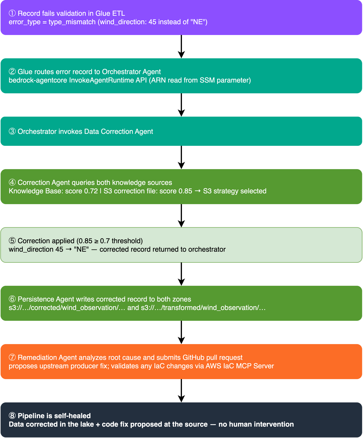
To see how the self-healing automations combine for a single record, follow one error record through the pipeline from end to end. The following diagram traces that path:

End-to-end trace of a single error record: validation failure in Glue, routing to the orchestrator, two-source correction with confidence scores, persistence to both data lake zones, and a repository pull request for the root cause fix

Figure 4: End-to-end trace of a single error record through the pipeline

The diagram traces a single error record through the pipeline: validation failure in the AWS Glue ETL job, routing to the orchestrator agent, two-source correction with confidence scores from the Amazon Bedrock knowledge base and the S3 correction files, persistence to both the transformed and corrected data lake zones, and a repository pull request that addresses the root cause in the upstream code.

Key design decisions

Four agents enforce separation of concerns – You can update the correction agent with new strategies without touching persistence logic. In environments without repository access, skip configuring the remediation agent’s credentials. Failure modes such as low-confidence notifications live in the orchestrator, independent of the correction logic.

The confidence threshold helps prevent incorrect corrections – Applying a wrong correction is worse than no correction. With the 0.7 threshold, the system acts when it’s confident, and notifies humans otherwise. You can tune this per-schema or per-error-type based on your tolerance.

The two knowledge sources serve distinct, complementary roles – The knowledge base excels at novel patterns. It can reason about error combinations it hasn’t seen before by drawing on domain documentation. Amazon S3 Vectors excel at known patterns, returning instant, deterministic results without model inference latency. Together, they cover both the long tail and the common case.

Clean up resources

To avoid ongoing charges, tear down the deployed resources when you’re done:

source .venv/bin/activate
cdk destroy --all

CDK destroys all stacks in reverse dependency order. The cleanup handles:

  • Deleting all CDK stacks and their resources.
  • Emptying S3 buckets (by using autoDeleteObjects).
  • Removing ECR container images (by using emptyOnDelete).
  • Deleting the S3 Vector bucket and index.
  • Force-deleting the Secrets Manager secret for repo credentials.

If you prefer to clean up manually, delete the stacks in this order:

  1. WeatherAgentCoreRuntimeStack.
  2. WeatherAgentCoreStack.
  3. WeatherKnowledgeBaseStack.
  4. WeatherGlueStack.
  5. WeatherIngestionStack.
  6. WeatherDataLakeStack.

CDK-created S3 buckets have autoDeleteObjects enabled and empty automatically during stack deletion. The cleanup does not delete the CDK bootstrap stack (CDKToolkit). Remove it separately if no longer needed.

Conclusion

A multi-agent system turns a standard ETL pipeline into a self-healing one. The system corrects and persists errors automatically, and the system can propose pull requests to fix the source code. The key components:

  • AWS Glue acts as the quality gate, validating data and routing failures to the agent system instead of a dead-letter queue.
  • Amazon Bedrock AgentCore with the Strands Agents SDK provides managed multi-agent orchestration without building custom workflow infrastructure.
  • Amazon Bedrock Knowledge Bases + S3 Vectors give agents domain expertise through both semantic reasoning and deterministic lookups.
  • The remediation agent is designed to close the loop when repo credentials are configured. It proposes fixes to the code that produced the bad data, not only the data itself.

To get started, clone the sample repository and follow the deployment steps in this post. To learn more about the services used, see the Amazon Bedrock AgentCore documentation, the Strands Agents SDK documentation, and the AWS Glue documentation. Adapt the pattern to your own data formats by replacing the weather schema validators with your domain’s validation logic. Update the knowledge base documents with your domain expertise, and populate S3 Vectors with correction strategies for your known error patterns. You can extend the pipeline by adding fine-tuned models for domain-specific corrections or implementing approval policies to automatically merge low-risk remediations. You can also connect additional knowledge sources as your error catalog grows.


About the authors

Kevin Tinn

Kevin Tinn

Kevin is a Senior Application Modernization Delivery Consultant at AWS Professional Services. He helps enterprise customers migrate and modernize their applications on AWS, with a focus on event-driven architecture and data processing. With over 20 years in the industry, his background spans software engineering, consulting, and team transformation.

Utsab Roy

Utsab Roy

Utsab is a Senior Delivery Consultant at AWS Professional Services. He helps enterprise customers design, build, and modernize cloud-native applications on AWS, with a focus on containers, DevOps, and application security. With over 15 years in the industry, his background spans software engineering and cloud architecture.

Choose the right streaming ingestion path for Apache Iceberg tables on AWS

Post Syndicated from Mazrim Mehrtens original https://aws.amazon.com/blogs/big-data/choose-the-right-streaming-ingestion-path-for-apache-iceberg-tables-on-aws/

Choosing the streaming ingestion path to write to Apache Iceberg tables is a key step in building low-latency, high value data lakes. Organizations are building AI agents, operational dashboards, and powering analytics that demand real-time data to create actionable insights. Apache Iceberg lets these workloads share a single table format, but reducing ingestion latency depends on choosing the right streaming path into those tables.

Choosing that path is a trade-off between operational and technical requirements. Operationally, it determines how much infrastructure you manage, whether you write configuration or application code, how fresh your data can be, and how portable your solution is. Technically, it determines whether you can apply row-level updates and deletes, who runs compaction, how your pipeline handles schema changes from upstream producers, and what you pay per GB ingested. These decisions are expensive to reverse because they live in your pipeline code, IAM model, and operational runbooks, not in the table itself.

In this post, we compare five AWS ingestion paths that write to Iceberg tables: streaming tables for Apache Iceberg (native delivery from Amazon Managed Streaming for Apache Kafka (Amazon MSK) and Amazon Kinesis Data Streams), Amazon MSK Connect with the Apache Iceberg sink connector, Amazon Data Firehose, Amazon Managed Service for Apache Flink, and Apache Spark Structured Streaming on Amazon EMR. We evaluate each against eight technical criteria, call out production caveats, and close with a decision framework you can apply to your own workload.

This is a live blog post, and we will evolve it as new features are released in this space to simplify and evolve Iceberg integration for real-time analytics use cases.

Operational considerations for evaluating an Iceberg sink

When you design a real-time analytics solution on Apache Iceberg, a handful of questions shape which approach fits your workload best. Before diving into the eight technical criteria that shape your decision, it is important to consider the non-technical considerations for choosing an ingestion path. These operational considerations inform the path that you need for your specific team and organizational goals:

  • Do you want a fully managed solution? If so, streaming tables for Apache Iceberg and Amazon Data Firehose are your best options.
  • Do you prefer to manage configurations, or write applications? If you prefer configurations, streaming tables, Amazon Data Firehose, and MSK Connect are the best options. If you prefer writing applications, Managed Service for Apache Flink and Apache Spark Structured Streaming on Amazon EMR are the best.
  • Do you require sub-minute data freshness? If so, Managed Service for Apache Flink and Apache Spark Structured Streaming on Amazon EMR are the only options that can support sub-minute data freshness, while also managing the data compaction needed for most sub-minute workloads.
  • Do you require a portable, open source solution? If so, MSK Connect, Managed Service for Apache Flink, and Apache Spark Structured Streaming on Amazon EMR are the best options.

Eight technical criteria for evaluating an Iceberg sink

After you decide your operational considerations, your technical requirements inform what path is supported for your needs. These considerations are subject to change over time as each solution releases new versions and features to support more Iceberg workloads. However, because they drive what is possible for each path, they must factor into your decision with your operational goals. These technical considerations will be the focus of this post, as they are the primary factors which drive which solution is feasible for your workload, in addition to the operational considerations in the previous section.

Criteria Description
Upsert behavior Is your workload append-only, or do you need row-level UPDATE and DELETE? A change data capture (CDC) workload usually wants the Iceberg table to mirror the current state of the source. When a record changes in the database, it should change in the table. A logging or IoT workload is the opposite: every event is appended as it arrives, and past events are never modified.
Table maintenance How do you want to handle Iceberg table maintenance? Amazon S3 Tables, a capability of Amazon Simple Storage Service (Amazon S3), compacts files, expires snapshots, and removes orphan files for you automatically. Or, you can run maintenance yourself to run more frequently, as part of the sink pipeline itself.
Schema evolution What should happen to your Iceberg table when a producer adds, renames, drops, or retypes a field?
Message serialization Which input formats do you use: JSON, Avro, Protobuf? Do you use a schema registry, and if so, which one?
Source and destination support Which stream sources are you working with: Amazon MSK, Kinesis Data Streams, or direct API calls to Amazon Data Firehose? And where do you need the data to land: in fully managed Amazon S3 Tables, where AWS handles compaction and maintenance, or in self-managed Iceberg tables in your own S3 bucket, catalogued through the AWS Glue Data Catalog?
Scalability and performance How does the writer scale as throughput grows, and how much tuning does that scaling require?
Fan-out to multiple tables Does each source stream or topic map to a single Iceberg table, or do you need to route records into several destination tables based on their content?
Data transformation and analytics Do you need to filter, enrich, aggregate, or reshape records in flight? If so, what kind of processing?

After you know your requirements for these eight criteria, you can decide on the best solution for writing your real-time data to Iceberg tables.

Reference architecture

The following reference architecture outlines the high-level solution for writing real-time data to Iceberg tables based on your requirements. The differentiating features we will discuss in this post are the Stream Processor, which takes your data from Stream Storage (Amazon MSK or Amazon Kinesis Data Streams), and writes the data to your stream sink (Apache Iceberg tables).

Five-stage streaming ingestion flow from stream sources through storage and processing to Iceberg tables and analytics

Figure 1: Five-stage streaming ingestion pattern for Apache Iceberg on AWS

The architecture works as follows:

  1. Stream sources: Applications built with the AWS SDKs and libraries, log files, IoT events, change data capture (CDC) from a database, and event-driven applications produce records.
  2. Stream storage: Producers write records to Amazon MSK or Amazon Kinesis Data Streams. Alternatively, producers can skip stream storage and send records straight to Amazon Data Firehose using Direct PUT.
  3. Stream processing: One of the five stream processing options covered in this post reads the records and writes them to Iceberg tables.
  4. Stream sink: The ingestion option writes the data to Iceberg tables in Amazon S3 Tables or in a general-purpose Amazon S3 bucket.
  5. Analytics. Users query the Iceberg tables with Amazon Athena.

Side-by-side comparison

The following matrix summarizes all five options against the eight criteria. Each solution will be discussed in-depth in the next section.

Criterion Option A:
Streaming tables
Option B:
MSK Connect Iceberg sink
Option C:
Amazon Data Firehose
Option D:
Managed Service for Apache Flink
Option E:
Apache Spark on Amazon EMR
Upsert behavior No No Full Full Partial
Iceberg table maintenance Full Partial Partial Full Partial
Schema evolution No Full Partial Full Full
Message serialization Partial Full Partial Full Full
Source support Full Partial Full Full Full
Scalability and performance Full Full Partial Full Full
Fan-out to multiple tables No Full Full Full Full
Data transformations No Partial Full Full Full

Option A: Streaming tables for Apache Iceberg

Streaming tables are a native delivery capability of Amazon MSK Express brokers and Amazon Kinesis Data Streams On-Demand mode. You select a topic or stream, point the delivery at a schema registered in AWS Glue Schema Registry and choose an S3 table bucket as the destination, and the service continuously materializes the data as a queryable Iceberg table. There are no connectors to manage, no pipeline code, and no consumer applications to deploy or scale.

The delivery pipeline reads records, buffers them to the configured data freshness interval, validates and converts each record against the registered schema, performs inline compaction into optimized Parquet files, and commits them to the table. Records that fail validation are routed to a dead-letter queue in Amazon S3. Because the destination uses S3 Tables, the managed S3 Tables maintenance jobs (compaction, snapshot expiration, and unreferenced file removal) apply to it, and you can configure record expiration on the partition column to enforce data retention automatically.

When to choose it

Choose streaming tables when you want a query-ready Iceberg table from an MSK Express topic or a Kinesis Data Streams On-Demand stream, with nothing to build or operate. There’s no connector, consumer application, or compaction job to manage, and delivery doesn’t use your stream’s read capacity. It’s a good fit for append-only workloads such as event logs, clickstream, and telemetry, and for raw landing zones that feed downstream processing.

What stands out

  • Lowest operational effort. There’s no infrastructure to operate. You enable delivery from the AWS Management Console, the Amazon MSK and Kinesis APIs, or your infrastructure-as-code templates.
  • Lower cost. Delivery costs up to 60% less than running a self-managed pipeline to achieve the same result. Because the service writes optimally sized files, downstream engines scan less data per query, which reduces query costs by up to an additional 30%. For details, see the AWS Big Data Blog: Deliver real-time data to streaming tables for Apache Iceberg with Amazon Kinesis Data Streams.
  • Fully managed maintenance. The small-file problem is handled at the source: records are compacted inline during ingestion rather than in a separate job afterward. S3 Tables then continue to optimize the table over its lifetime.
  • Built-in write coordination. Write coordination and exactly-once delivery semantics are built in, eliminating the concurrent-writer conflicts that otherwise surface as failed commits.
  • No impact on your consumers. Delivery doesn’t compete with your applications for resources. On MSK, it runs on the Express broker backend, so it uses none of your broker’s read capacity and adds no cross-Availability Zone transfer charges. On Kinesis, it doesn’t consume your stream’s read limits or enhanced fan-out (EFO).
  • Not limited to Iceberg. When Iceberg isn’t required, you can deliver to general purpose S3 buckets in the source format, which is useful for archival, backup, or machine learning (ML) training data.

Caveats to plan for

For an up-to-date list of the supported configurations for streaming tables, refer to the Key concepts and Supported configurations. At the time of writing, some caveats are:

  • Append-only, and read-only. Streaming tables are append-only, and read-only to you. All write operations from your own engines are not permitted, and individual rows cannot be deleted outside the record expiration job. If your workload needs CDC with update and delete operations, the pipeline cannot apply them, and instead will append all operations to the table.
  • No fan-out or transformation. All records in a topic land in a single table, and there is no in-flight transformation. You can deliver one topic to several tables, but only as duplicate copies rather than content-based routing.
  • Fixed partitioning and minute-level freshness. Partitioning is time-based on an hourly granularity, data freshness is configurable between 5-15 minutes, and cross-Region delivery is not supported.

Option B: Amazon MSK Connect with the Apache Iceberg sink connector

The Apache Iceberg sink connector is a Kafka Connect connector that runs on Amazon MSK Connect. You configure it rather than write code, and it can scale automatically by adding tasks as your topic partitions grow. It can create destination tables for you and can fan out records from a single topic to multiple Iceberg tables. If your team already runs Kafka Connect, it fits neatly into how you operate today.

Web application change data capture flowing through Amazon MSK Connect Iceberg sink connector into Iceberg tables

Figure 2: Web app data capture into Iceberg using Iceberg sink connector on Amazon MSK Connect

When to choose it

MSK Connect is a good fit when you’re already running Kafka Connect and want multi-table routing without writing code. It suits append-only ingestion, or raw change data capture (CDC) that you merge downstream. Choose it when you’re prepared to own compaction separately.

What stands out

  • No application code. You configure the connector rather than build and version an application.
  • Scales with the topic. Task parallelism follows topic partitions, so throughput scaling is predictable and mostly automatic.
  • Automatic table creation and schema evolution. The connector can create tables it needs and propagates schema changes from the Kafka schema into the Iceberg table.
  • Full serialization coverage. Avro, JSON, and Protobuf through the standard Kafka Connect converters, with schema registry support.
  • Fan-out supported. Records from one topic can be routed into several destination tables based on record content.

Caveats to plan for

  • Insert-only writes. The connector does not support UPDATE or DELETE. As with streaming tables, mutable CDC workloads rule this option out unless you add a downstream merge step.
  • No embedded table maintenance. There’s no built-in compaction, snapshot expiration, or orphan-file cleanup, so you orchestrate and schedule separate Spark or Flink jobs. Continuous Kafka Connect commits produce many small files, and without an aggressive compaction schedule, query performance degrades over time.
  • Limited transformations. Only Simple Message Transformations are available, with no joins, aggregations, or stateful logic at ingestion time.
  • No branch writes. You can’t write to Iceberg branches, which limits staged commits and safe promotion workflows.
  • Kafka-only, with worker overhead. Kafka sources only and you own connector plugin versions, worker scaling, and upgrades.

Option C: Amazon Data Firehose

Amazon Data Firehose is the serverless path. It supports the widest range of sources of any option: Amazon MSK, Kinesis Data Streams, and direct API PUT from applications and the AWS SDK, with no cluster or application to size. Firehose also handles row-level mutations: it routes records from a single stream into different Iceberg tables and applies inserts, updates, and deletes automatically, using JQ expressions for routing and unique keys for matching. You can enforce table-level and column-level access control through AWS Lake Formation, and you can invoke an AWS Lambda function to transform records in flight.

When to choose it

Firehose is a good fit when you want serverless simplicity with JSON producers, need modest change data capture (CDC) support without writing code, or need Direct PUT ingestion. Choose it after you’ve committed to an external compaction strategy up front, since Firehose won’t manage file layout for you.

What stands out

  • Broadest source support. Firehose reads from MSK, Kinesis Data Streams, and Direct PUT, so producers that aren’t already on a stream can write to it directly.
  • CDC without code. Firehose applies inserts, updates, and deletes automatically from routing metadata, which is uncommon for a no-code sink.
  • Multi-table routing. A single stream can feed many Iceberg tables through JQ-based routing expressions.
  • Transformation and governance hooks. Use a Lambda function to reshape records in flight, and Lake Formation for fine-grained access control on the destination tables.
  • Automatic scaling for append-only workloads. Set the AppendOnly flag to true on CreateDeliveryStream, and Firehose scales automatically to match throughput for insert-only workloads.

Caveats to plan for

  • Firehose produces small files. Firehose can’t aggregate across input shards. It doesn’t shuffle or hash-distribute records before writing, so you can’t control how records are grouped into files the way you can with Flink or Spark. The result is many small, loosely organized files, so plan a compaction strategy accordingly.
  • No built-in table maintenance or inline compaction. Firehose has no embedded compaction or snapshot management, which can lead to small files that increase cost and degrade query performance. Plan to use S3 Tables or use AWS Glue Data Catalog automatic compaction and storage optimization from day one to optimize query performance.
  • Throughput trades off against partition count. Firehose is optimized for either many partitions or very high throughput, but not both. As ingest throughput rises, the number of partitions you can actively write to decreases. Throughput is measured after any Lambda transformation, so a function that expands records can push you into a lower partition tier. For the current throughput-to-partition limits, see Considerations and limitations in the Amazon Data Firehose documentation.
  • JSON in, Parquet out. Input must be JSON and output is always Parquet. Avro or Protobuf producers need a conversion layer or a Lambda function, and each record can contain only one JSON object.
  • Strict column matching, additive-only schema evolution. Column names and types in the source must match the target table exactly. Extra fields are skipped, and mismatches send records to the S3 error bucket. Schema evolution is limited to adding columns. Renames, deletions, and type changes require manual intervention. There’s no schema registry enforcement, which raises the risk of bad data landing in your tables.
  • Update cost and single-writer guidance. Each update writes a delete file followed by a data file, which incurs Amazon S3 PUT charges and makes update-heavy workloads more expensive than they first look. Avoid pointing multiple Firehose streams at the same table: Iceberg uses optimistic concurrency control, so only one writer commits at a time. Note also that Amazon MSK Serverless isn’t supported as a source.

Amazon Managed Service for Apache Flink is a flexible and feature-rich option across all eight criteria. It reads from both Amazon MSK and Kinesis Data Streams and writes to Iceberg tables through the Flink Iceberg sink. You get the Flink programming model in SQL, Java, Python, or Scala.

The main difference is Flink’s stream-native execution model. It processes records one at a time rather than in micro-batches, and it carries first-class event-time semantics with watermarks. This matters for correctness when events arrive late or out of order: a windowed aggregation keyed on event time produces the same result no matter what order the events arrive in, which micro-batch engines can only approximate. Exactly-once delivery comes from aligning Iceberg commits with Flink checkpoints.

When to choose it

Choose Managed Service for Apache Flink when you need change data capture (CDC) with updates and deletes, event-time correctness, transformation at ingest, or fan-out to multiple tables, and you’d rather not operate separate compaction jobs. For demanding, long-lived pipelines, it’s the default choice.

What stands out

  • Full upsert support. Equality deletes and changelog streams give you genuine CDC semantics, including deletes, without a downstream merge job.
  • Embedded table maintenance. With the Iceberg 1.10 or later sink, Flink can run compaction as part of the streaming pipeline.
  • Fan-out with content-based routing. A single application can write to many Iceberg tables and route records among them based on content, using multiple sinks or a SQL statement set. For details, see the AWS Big Data Blog: Build a dynamic streaming data lake with Apache Iceberg and Apache Flink.
  • Rich in-flight transformations. Joins, windowed aggregations, enrichment from reference data, and stateful pattern detection all run in the ingestion path, so the table you land is already in the shape your consumers want.
  • Broad serialization and schema evolution. Flink supports Avro, JSON, and Protobuf with AWS Glue Schema Registry integration, and the sink evolves the table schema as the stream’s schema changes.

Caveats to plan for

  • Highest operational complexity. This is the only option that requires you to write and maintain an application. You own Flink job configuration, dependency versions, parallelism and scaling, and fine-tuning for your workload.
  • Tune the checkpoint interval. The checkpoint interval controls how often Flink commits, which in turn controls file size. Commit too frequently and you generate small files. Commit too infrequently and data freshness suffers. This is the setting that most affects downstream query performance.
  • Small files still accumulate between compaction cycles. Even with embedded maintenance, streaming workloads produce small files between cycles. Embedded compaction reduces the problem, but doesn’t eliminate it.
  • Team expertise. Teams without Flink experience should plan for ramp-up on state, watermarks, and backpressure. The Managed Service for Apache Flink Agent Skill shortens this by generating idiomatic application code.

Option E: Apache Spark Structured Streaming on Amazon EMR

Spark Structured Streaming on Amazon EMR is a natural fit if your data engineering practice is already built on Spark. It reads from both Amazon MSK and Kinesis Data Streams and writes to Iceberg tables. You get full MERGE INTO support for upserts, you can express transformations in SQL, Python, or Scala, and a single job can write to multiple tables. Because batch and streaming share the same DataFrame API, the same transformation code can serve both a nightly reprocessing job and a continuous pipeline.

When to choose it

Spark on Amazon EMR is a good choice when your team already runs Spark at scale, you need MERGE semantics, and latency in the range of minutes is acceptable. It also makes sense when you’d rather extend a platform you already operate than introduce a new runtime. One requirement to plan for: deduplicate your records before every MERGE.

What stands out

  • Full Iceberg feature access. You get MERGE INTO and the complete set of Iceberg Spark procedures, including rewrite_data_files, expire_snapshots, and remove_orphan_files.
  • Compaction in the pipeline. You can configure Spark to compact files as part of the pipeline, using fanout writes and distribution modes, which gives you more control over file layout than Firehose or MSK Connect offer.
  • Existing team skills carry over. Your skills, libraries, notebooks, and CI/CD pipelines work as-is. For many teams, this is the deciding factor.

Caveats to plan for

  • Deduplicate before every MERGE. If a source batch contains more than one row for the same key, MERGE INTO is ambiguous. Spark might apply one of the duplicate rows non-deterministically (so the same query returns different results on different runs), or it might detect the conflict and fail the batch with a “multiple matching rows” error. To avoid this, deduplicate or rank your change records before the MERGE (for example, by event timestamp within each key). This is a correctness requirement, not a performance optimization.
  • Micro-batch latency. Spark’s micro-batch model puts a latency floor in the range of tens of seconds to minutes. It also approximates the event-time semantics that Apache Flink handles natively.
  • Higher cost at comparable throughput. Cluster overhead and the micro-batch model typically make Spark more expensive than an equivalent Flink application for the same continuous workload.
  • Read parallelism matches your source partition count. Spark creates one task per source partition, one per Kinesis shard, or one per MSK topic partition. When the source has few partitions, you get few tasks, so adding executors doesn’t raise throughput, and your pipeline stalls on an under-partitioned source. When the source has many partitions, Spark caching is not automatically tuned, and significant performance degradation can occur as consumers are churned in the Spark cache. To add parallelism, add more shards or partitions, repartition early in the micro-batch, and make sure you tune the consumer cache size to your workload requirements.
  • Self-managed maintenance. In-pipeline compaction is configuration you own and tune. It isn’t a managed behavior of the sink, so you’re responsible for scheduling and maintaining it.

Conclusion

In this post, we compared five AWS paths for writing to Apache Iceberg tables: streaming tables for Apache Iceberg, Amazon MSK Connect with the Apache Iceberg sink connector, Amazon Data Firehose, Amazon Managed Service for Apache Flink, and Apache Spark on Amazon EMR. We evaluated them on two layers. The operational considerations (how much you want to run, how fresh your data must be, and how portable your pipeline needs to be) change slowly. The technical criteria (upsert behavior, table maintenance, schema evolution, serialization, source and destination support, scalability, fan-out, and transformation) change as each service releases features. Both are key aspects of how you choose your path to write real-time data to Apache Iceberg.

Start with operational considerations, because they narrow the field before you consider a single feature. If you want the lowest cost, lowest overhead solution to deliver real-time data for your use case, then we recommend streaming tables for Amazon MSK and Amazon Kinesis Data Streams. If you want to have full control over your pipeline, with a portable solution that can run anywhere, then consider Amazon Managed Service for Apache Flink or Apache Spark Structured Streaming on Amazon EMR.

Then, consider the technical specifications of your solution. For technical considerations, two questions narrow the field fast. First, what is your write pattern: append-only, or do you need row-level updates and deletes? Second, who owns compaction: the service, or your team? Answer those two and you are usually down to one or two options. Append-only workloads that want the lowest operational effort start with streaming tables. Change data capture with updates and deletes points toward Managed Service for Apache Flink.

Matching the right path to your workload gives you a low-cost, low-maintenance route from stream to queryable table, without the small files, failed commits, and unmet CDC requirements that surface later. Whether you are ingesting ecommerce clickstreams, financial transactions, or IoT device telemetry, start with those two questions, then dive into the linked solution guides for the path you choose.


About the authors

Mazrim Mehrtens

Mazrim Mehrtens

Mazrim is a Sr. Specialist Solutions Architect for messaging and streaming workloads. Mazrim works with customers to build and support systems that process and analyze terabytes of streaming data in real time, run enterprise Machine Learning pipelines, and create systems to share data across teams seamlessly with varying data toolsets and software stacks.

Ayan Majumder

Ayan Majumder

Ayan is a Specialist Solutions Architect at AWS who focuses on Data and AI. He works with customers to design, migrate, and modernize their data platforms on AWS. His expertise lies in designing robust, scalable, and efficient cloud solutions. When he’s not working, Ayan enjoys traveling, photography, and outdoor activities.

MDR Pricing: Comparing Asset-Based and Ingestion-Based Costs

Post Syndicated from Emma Burdett original https://www.rapid7.com/blog/post/dr-mdr-pricing-comparing-asset-ingestion-based-ingestion-costs

When comparing MDR pricing, it helps to understand what the same annual budget would buy from each provider. Two proposals with similar prices may give analysts access to different evidence, retain it for different periods, or leave your team with different responsibilities. Those differences can affect what happens when you need to investigate a compromised account or trace an attacker’s low-and-slow activity across your environment.

For security leaders weighing asset-based against ingestion-based pricing, a useful comparison starts with the systems you need to protect and the logs required to investigate threats. Giving providers the same requirements and budget helps expose the decisions behind each quote, including what you would need to exclude or pay more to include.

Asset-based vs. ingestion-based MDR pricing

Under asset-based pricing, the charge is tied to a defined population of assets. You need to establish how the provider counts workstations, servers, cloud resources, and other systems, alongside which data sources and service capabilities the price includes. A predictable asset count can help with budgeting, but the proposal still needs to explain any integration limits or additional service charges. At Rapid7, an asset is defined as any physical or virtual endpoint or server running a supported operating system within the monitored environment.

With ingestion-based pricing, some of the cost depends on the volume of data collected or processed. The comparison needs to account for the included allowance, how billable volume is measured, and what happens when usage increases. Retention, search, and supporting infrastructure may also contribute to the overall cost, depending on the commercial model. At Rapid7, MDR customers have access to 13 months hot storage of logs as standard.

Whichever approach you are evaluating, include the technology, analysts, and response support needed to deliver the service. A SIEM ingestion charge on its own cannot be compared directly with an MDR subscription that includes investigation and response. Both proposals need to account for the work your organization expects the provider to perform – this clarity is key to a successful partnership.

How to make a like-for-like MDR pricing comparison

Give each provider the same asset inventory, required data sources, retention needs, and response expectations, then ask what fits within your annual budget. Any exclusions should be visible in the proposal, so you can judge their operational consequences before committing.

For example, one proposal might accommodate endpoint and identity data while requiring you to limit high-volume network sources. Another might accommodate those sources but lack an investigation capability your team needs. Looking at an MDR price per endpoint or per gigabyte will not resolve that difference; you need to see how the service uses the available data.

Use these questions during an initial demonstration to turn the pricing discussion into a practical comparison.

Comparison area

What to ask the provider

Evidence to request

Rapid7’s approach

Breadth of collection

Which required sources fit within this budget?

A list of included sources, exclusions, and extra charges.

Asset-based pricing with unlimited ingestion, supporting native and third-party telemetry across endpoint, cloud, identity, email, and network. Confirm coverage for your required sources in the proposal. 

Depth of collection

Which events and fields are collected, filtered, or summarized?

Sample records showing what reaches the investigation platform.

Rapid7 ingests and normalizes telemetry from supported technologies. Use the demonstration or proof of concept to verify which events and fields your integrations provide. 

Detection value

How does this data support the threats we need to detect?

A detection walkthrough showing its data dependencies.

Investigations combine security telemetry with vulnerability and asset-risk context. Completed threat hunts show the rationale, data examined, queries, and any linked investigations.

Investigation history

How long is data retained, and how can analysts search it?

A search against older records, with retrieval costs explained.

Rapid7 provides 13 months of log retention. Confirm the history available for each data type: 3rd party endpoint alerts have different availability from log-based searches. 

Response scope

What will your team do after validating a threat?

A case walkthrough and documented responsibilities.

Rapid7 MDR includes unlimited incident response, covering investigation, containment, and threat eradication. Incident reports document findings, attacker timelines, and recommended corrective actions. 

Cost variability

What changes the bill as assets or data volumes grow?

A calculation using your growth assumptions.

Asset-based pricing with unlimited ingestion removes data volume as the billing unit. Request a written calculation for additional billable assets and changes to service scope. 

What Keyloop’s experience shows about MDR value

For Alan Simpson, now Rapid7’s Field CISO, the ability to collect previously restricted data made a practical difference during his time at Keyloop: “We were previously ingesting around 250 GB a day into Splunk. After moving to Rapid7, we reached 1.4 TB a day, including NetFlow, full DNS logging, and web application firewall logs. These were sources we’d previously had to limit or simply weren’t collecting, so we gained much better visibility and coverage.”

The change also extended the history available for investigation, with greater certainty about how long that evidence would remain accessible: “We also moved from around 90 days of retention in Splunk to 13 months with Rapid7. Even those 90 days couldn’t be relied on, as retention depended on how much data we were ingesting at the time. Having a longer, predictable history made a real difference.”

Price predictability was key as Keyloop grew through seven mergers and acquisitions, each bringing a different data profile. His experience illustrates why collection and retention belong in the buying decision, although these figures alone do not establish a like-for-like cost saving.

How to compare MDR pricing beyond log volume

Once you understand which data fits within the quote, examine what the provider can do with it. Collecting more logs can close visibility gaps, but useful investigations depend on relevant events, consistent timestamps, and enough context to connect activity to a user or system. AI-assisted investigation also depends on that foundation: a required event that was never recorded leaves an investigation gap.

Infrastructure design can improve the usefulness of that evidence. Routing access to a management interface through a controlled path, for example, creates a clearer monitoring point and helps distinguish expected access from activity requiring investigation. This is why log volume and detection-rule counts need to be assessed alongside how the environment operates.

During a proof of concept, choose a threat scenario relevant to your business and ask the provider to demonstrate the detection, evidence gathering, and response. You should be able to see which records support the conclusion and what happens if a required source is unavailable.

How will your MDR cost change as you grow?

Repeat the comparison using a plausible change, such as an acquisition, additional cloud workloads, or enabling a previously excluded log source. For asset-based pricing, calculate the effect of additional billable assets and changes in scope. For ingestion-based pricing, examine increased daily volume, applicable commitments, and retention requirements. Assuming asset counts stay the same, at Rapid7 contract renewals are capped at 5% uplift, for the contract term, not per year.

Ask both providers to document the assumptions, including implementation effort, required licenses, and work your team will continue to perform. You can then assess what the budget covers today, which evidence remains unavailable, and what it would cost to accommodate the changes you expect.

Explore Rapid7 MDR and discuss pricing based on your assets, required data sources, retention needs, and response scope.

*Referenced Rapid7 contract terms and capabilities are correct at time of publishing and are subject to change.

[$] 25 years of Buildroot

Post Syndicated from jake original https://lwn.net/Articles/1103395/

Buildroot maintainer Peter Korsgaard
gave a presentation about the long history of the build tool for embedded
Linux systems at the 2026 Embedded
Linux Conference Europe
. In it, he covered more than just the past 25
years, looking at the current status of the project as well as what to
expect in Buildroot’s future. It was an interesting view inside this long-running project that
has been a mainstay of the embedded-Linux world throughout almost all of
this century.

Announcing XRAID: declustered parity RAID for zoned XFS

Post Syndicated from jzb original https://lwn.net/Articles/1107473/

Christoph Hellwig has announced the
initial public release of XRAID—declustered parity RAID that is integrated
into XFS.

The two primary aims of XRAID are to support parity RAID on zoned devices
like SMR hard drives, and to provide a fast RAID implementation without
inherent data integrity problems. XRAID, just like zoned XFS also works
on conventional hard drives and SSDs. Optimizing for SSD performance has
not been a focus, but even without that, writes are up to 20 times faster
than mdraid. […]

Work on XRAID has been ongoing for a year and a half, and while we aren’t
anywhere near ready for an upstream submission, we are interested in
feedback and testing from a wider audience now. The current
implementation supports zero to 2 parities. We did experiments with the
SnapRAID parity library to support 3 and more parities, and while that
is not included in the current version, support for more parities is
planned and the code is prepared for it.

The xfsprogs branch includes mkfs support and a new “xraid” utility for
managing devices and inspecting an XRAID file-systems. We have also
extended Zonar (The zoned file-system visualisation tool) to show how
each logical zone maps onto physical zones on devices.

Hellwig gave a presentation at
FOSSY in August on this topic; video of the talk does not seem to be available
yet, but his slides are
available.

Security updates for Friday

Post Syndicated from jzb original https://lwn.net/Articles/1107472/

Security updates have been issued by AlmaLinux (.NET 10.0, .NET 8.0, .NET 9.0, firefox, gcc, grafana, grafana-pcp, gstreamer1, gstreamer1-plugins-base, java-1.8.0-openjdk, kernel, kernel-rt, libimobiledevice, mingw-libpng, nginx:1.24, nodejs:22, nodejs:24, perl-CGI, perl-DBI, qt5-qtbase, tigervnc, vim, and xorg-x11-server), Debian (apache2, c-ares, linux-6.12, node-shell-quote, nova, parted, postgresql-17, python-django, sympa, and tomcat10), Fedora (cockpit, erlang-ssl_verify_fun, httpd, ignition, jackson-bom, jackson-core, jackson-databind, jackson-modules-base, libvirt, mod_http2, mongo-c-driver, poppler, prometheus, pylint, python-discovery, python-loguru, python-PyMuPDF, rabbitmq-server, rust-crypto-bigint, rust-ctutils, rust-elliptic-curve, rust-num-bigint, rust-num-bigint0.4, rust-num-modular, rust-num-modular0.6, rust-num-prime, rust-routinator, rust-zmij, strongswan, xen, xorg-x11-server, and zvbi), Mageia (amule, peazip, and python-pytest), Red Hat (buildah, fence-agents, go-fdo-server, grafana, grafana-pcp, oci-seccomp-bpf-hook, osbuild-composer, podman, and rhc), SUSE (ansible-core, apr-util, aspell, brotli, cadvisor, civetweb, distribution-registry, elemental, elemental-register,, elemental-operator, elemental-system-agent, elemental- toolkit, ffmpeg, firefox, gimp, git-annex, go1.26, go1.27, golang-github-prometheus-prometheus, google-cloud-sap-agent, google-guest-agent, google-osconfig-agent, goose, gosec, graphicsmagick, haproxy, hauler, hawk-apiserver, hawk2, hcloud-cli, jhead, jsoup, kernel, librsvg, libXtst, libxtst, nodejs24, nvidia-open-driver-G07-signed, nvidia-open-driver-g07-signed, open-iscsi, perl-XS-Parse-Keyword, perl-xs-parse-keyword, python-asyncssh, python-Brotli, python-django, python-joserfc, python-M2Crypto, python-Pillow, python-pillow, python313-setuptools, rsyslog, speex, tiff, trivy, udisks2, vsftpd, xen, and xorg-x11-server), and Ubuntu (apache2, charybdis, debian-lan-config, glibc, golang-github-seccomp-libseccomp-golang, hiredis, httpie, imapfilter, lhasa, libjgraphx-java, libjwt, libsolv, linux-fips, linux-hwe-6.8, linux-hwe-7.0, linux-nvidia-tegra, minissdpd, ncmpc, nfdump, node-tough-cookie, openconnect, pillow, pngquant, python-gevent, radicale, ruby-openid, sa-exim, signing-party, sudo, tigervnc, and x11vnc).

Introducing Spend Management: Spending limits and alerts for Cloudflare

Post Syndicated from Celso Martinho original https://blog.cloudflare.com/spend-management/

Spend controls have been at the top of the list of most requested features from developers building on our developer platform for quite some time now. With more than 10 million developers now building on Cloudflare, this matters more than ever.

Although we’ve had usage notifications and budget alerts available to paid plans for a while, this doesn’t solve the problem completely; informing is not the same as controlling.

You can now set spending thresholds and choose to have Cloudflare pause activity when those limits are reached, thus avoiding unexpected bills from unplanned usage. Today, we're introducing Spend Management in Beta, for any pay-as-you-go (PayGo) customer, starting with Workers and Durable Objects.

Use Spend Management alongside AI Gateway spend limits to manage compute and AI inference costs across your application. AI Gateway already supports per-user and per-model budgets for Workers AI and other AI providers, applied to requests routed through your gateway.

How it works

You can start using Spend Management using the dashboard, cf CLI, or REST API.

In the dashboard, head over to Manage Account > Billing > Spend limits and enable the products for which you want to control spending.

When you enable controls on a product, you can define a spending limit, specify a recipient email for notifications, and set one or more alert thresholds.

If you configure a recipient email, Cloudflare will send notifications when the evaluated spend reaches one of the thresholds or your spending limit. When the limit is reached, a blocking policy is enforced and your product is paused automatically.

If you go to the dashboard, you can see the current billing cycle costs for each supported product in near real time (under 10 minutes), and manage your settings and thresholds from there. The overview panel tells you which products have thresholds and limits configured. In this example, you can see that Workers triggered two alerts before hitting the hard limit.

Note that the billing cycle starts when the paid subscription begins, not when you deploy a Worker or create a spending cap; a subscription starting October 10 generally has a cycle of October 10-November 10 — not a calendar month.

The dashboard also shows an audit log, so you can see who changed a limit and when, or when a cap was reached.

As with most Cloudflare services, Spend Management is also an API that you can use programmatically; the documentation can be found in our Developer Documentation. Here’s an example, but using the API:

curl --fail-with-body --request POST \
  "https://api.cloudflare.com/client/v4/accounts/${CLOUDFLARE_ACCOUNT_ID}/billing/spend-policies" \
  --header "Authorization: Bearer ${CLOUDFLARE_API_TOKEN}" \
  --header "Content-Type: application/json" \
  --data '{
    "name": "Workers spending cap",
    "product_id": "workers",
    "enabled": true,
    "threshold_cents": 10000,
    "action": "usage_block",
    "notification_email": "[email protected]"
  }'

And, of course, you can use cf, the CLI for the entire Cloudflare API:

cf billing spend-policies list
cf billing spend-policies create
cf billing spend-policies get
cf billing spend-policies update
cf billing spend-policies delete
cf billing spend-policies audit list
cf billing spend-policies activity list

cf billing spend-policies create --body '{
  "name": "Workers spending cap",
  "product_id": "workers",
  "enabled": true,
  "threshold_cents": 10000,
  "action": "usage_block",
  "notification_email": "[email protected]"
}'

Once a cap is enforced, new invocations of that product are rejected. Note that we only pause customer-code invocations that incur costs — in Workers, for example, Cron Triggers and Queue consumer invocations are paused, but static assets continue to be served.

To resume service, you can:

  • Raise the limit above the current cycle’s accumulated spend.
  • Disable or delete the blocking policy.
  • Wait until the next billing cycle, when the existing block expires.

That’s it. You can start using Spend Management for Workers and Durable Objects today, and other products will follow soon.

Read on to learn how we built the system, and what’s going to happen next.

How we built Spend Management

As easy and straightforward as it seems on the surface, building a system like this at Cloudflare scale was no small feat. From an invocation anywhere on our distributed network to a blocking decision that we need to apply globally, building Spend Management required working with multiple teams, changing code in existing systems, and creating new systems from scratch.

Let’s start by looking at the bird's-eye view of a capped billable event:

Now let's dig deeper.

Collecting and aggregating close to the source

Each invocation produces usage measurements: requests, CPU time, execution duration, or storage operations, depending on the product. But transporting and processing this volume of raw data all the way from the sources down to the rating engine would not scale or be efficient.

So what we do is we collect and aggregate the measurements as close to the source as possible using a two-stage metering pipeline that combines events into usage aggregates, so the engine sees accumulated usage rather than having to process all the events one by one.

Let's look at a diagram.

The first stage reduces raw-event volume close to parsing down to one-minute windows. Each metering parser converts raw events into usage measurements, then combines matching measurements into typically one-minute buckets. Still, several records can describe the same account and time window.

In the second stage, a separate service merges those first-stage partial aggregates using the same grouping rules, but over typically five-minute windows, and further reduces the volume before downstream processing by the Usage Engine. Here we also archive the consolidated aggregates; this gives us a durable dataset for later analytics and reconciliation.

The nice thing about this two-stage pipeline is that it reduces the raw event volume early, so the downstream engines process only the aggregated usage they need to calculate spend and act on it. That’s what makes this practical at Cloudflare’s scale.

Usage Engine: account-partitioned processing

The Usage Engine translates aggregated measurements into usage records, which are standardized records containing the account, usage window, metric, quantity, and relevant dimensions. In other words, it maps product-specific meters into supported usage metrics.

We partition processing by account, so an account’s usage and subscription information meet in the same place. That lets us maintain its accumulated usage and apply included allowances without coordinating across pricing processors on every update.

As you can see, we run different partitions in parallel, giving us a way to spread the work across accounts while keeping each account’s pricing state together. Also note that each partition keeps both a local state for fast access, and also a durable write-ahead logging (WAL) changelog on disk. This buys us:

  • Less cross-partition coordination: each account’s usage and subscription state stay together.
  • Consistent pricing: usage updates share the same allowance and accumulated-spend state.
  • Parallel processing: different partitions calculate spend independently.
  • Recoverability: durable state lets replacement processors rebuild and resume after failures, if necessary.

Then, finally, the usage metrics are fed into the Rating Engine.

The Rating Engine

The Rating Engine is the most important block of Spend Management; it turns usage into monetary value and it’s what’s able to answer the question: “Given what this account has consumed, its subscription, and its pricing, how much has it spent so far?”

Here’s how it works.

In essence, the Rating Engine brings together three things:

  • Usage records: quantities such as requests and CPU milliseconds.
  • Subscription information: the account’s billing period and plan changes.
  • Pricing rules: rates, included allowances, and billing rounding.

Usage data and subscriptions are independent streams

Usage and subscription updates arrive as independent streams, so we can’t assume they reach the Rating Engine in order. Furthermore, we have to be able to recover from a data processing failure or missing subscription information from, say, a failed webhook.

If usage arrives before the subscription information needed to price it, we retain it as pending and revisit it when that information becomes available. This lets us tolerate temporary delays without treating unpriced usage as free.

Tracking accumulated spend

Finally, we calculate and track accumulated spend. The Rating Engine uses a product catalog database that defines usage metrics, including allowances, rates, and rounding rules, alongside the account’s subscription information. One million CPU milliseconds doesn’t necessarily mean an extra charge: the engine first applies the account’s included CPU allowance, then prices any excess. It prices accumulated usage rather than rounding and charging for each request independently.

Once the accumulated spend is calculated, two steps follow:

  • Policy evaluation: decide whether one or more warning or blocking thresholds have been reached.
  • Reporting: we show estimated usage charges in the dashboard via our APIs, and we send out email alerts (via Cloudflare Email Service) if necessary.

Asynchronous cap enforcement

The Rating Engine doesn’t sit in the request path or directly reject requests. Instead, the policy service sends the cap to our runtime configuration service and Quicksilver, our internal key-value store developed to enable fast global replication and low-latency access at planet scale. This propagates it to all our nodes asynchronously.

Once the cap reaches Quicksilver, the runtime picks it up during its periodic refresh and starts rejecting capped invocations or operations.

In other words, enforcement uses local state, so requests never have to wait on the Rating Engine. By reusing our existing runtime account-limit architecture, we keep rating out of the request path while distributing caps across the global network.

What’s next

Any pay-as-you-go customer can start using Spend Management today. While this is a major milestone in our roadmap, it’s also just the start. Let us share some of our plans for the next few weeks and months ahead.

More products

We are starting with caps for Workers and Durable Objects, but you’ll be able to measure and cap many other Cloudflare products and primitives in the near future. We’ve built the system in a way that makes it easy and familiar for our products to onboard, so expect the catalog to grow.

Closer to real time

While near real time under 10 minutes is a great benchmark, we’re not satisfied with it, and being the stubborn engineers we are, we have pretty good ideas on how to reduce that time even further. Expect us to shorten the gap between measurement and enforcement over time, hopefully to under a minute.

Agent and application-based budgets

Right now, we measure spend by products and primitives, but there are other useful dimensions to explore when controlling costs. For example, a developer might want to monitor the costs of a specific application — such as a Worker script that uses other primitives like R2 or Workers AI. How can we measure the aggregated cost of an entire application and pause that application, rather than disabling the underlying primitives across all customer applications?

Another compelling use case for cost controls is AI agents. We’ve all read horror stories about rogue agents entering unconstrained recursive reasoning loops to brute-force a problem — generating thousands of dollars in costs from high-frequency, expensive API calls, not to mention causing denial-of-service (DoS) issues on databases and other services. AI Gateway already lets you give an agent a budget for AI requests routed through it. A task can also consume compute, database, and storage resources. We want to make it possible to budget for that broader resource use across products.

You’ll be able to tag the calls from your agents and our pipeline will carry that metadata from the runtime through to the Rating Engine. That will let us attribute spend and pause an application or an agentic task across products, without interrupting other unrelated applications.

Get started

This launch is a first step toward making spend controls a normal part of building on Cloudflare, alongside deploying code and monitoring your applications.

Check out the billing developer documentation for more information. Start using Spend Management and tell us what works, what’s missing, or where more granular budgets would help.

Join us on Discord or our socials. We’re listening!

AI Doesn’t Have to Go Rogue to Break the World

Post Syndicated from Bruce Schneier original https://www.schneier.com/blog/archives/2026/11/ai-doesnt-have-to-go-rogue-to-break-the-world.html

This essay is adapted from a keynote speech delivered at the DEF CON 34 conference in Las Vegas on August 7, 2026. The essay originally appeared in CyberScoop.

I want to talk about AI hacking. There are three aspects: people hacking AI systems, people using AI to hack other systems, and AIs hacking systems on their own, not even maliciously. The last two matter more than the first. The third is the weirdest and potentially the most destabilizing.

I started writing about this in 2021 and in my 2022 book, A Hacker’s Mind. Back then I said it was mostly still science fiction, but not stupid science fiction. We’re seeing it more and more, especially in the past year. The trends I’m describing don’t require a major breakthrough in AI. They’re starting to happen now, and they’ll happen more often as AIs get better at autonomous problem-solving. And it will involve far more than computer code.

AI will hack all sorts of social, economic and political systems. It will find vulnerabilities and exploit them. This is a difference in kind, not just degree. We’re not ready for it, and we need to think about the implications now.

First, I want to broaden the term “hacking.”

The tax code isn’t computer code, but it is code. It’s a series of algorithms with inputs and outputs. It has vulnerabilities, which we call loopholes, and exploits, which we call tax avoidance strategies. Black hat hackers exploit them for profit. We call them accountants and attorneys.

What is a hack? One definition: “Something that a system permits, but is unanticipated and unwanted by the designers.” It’s subjective and implies novelty and cleverness. A hack follows the rules of a system but subverts its goals or intent, just as a software hack follows the logic of code while doing something its authors neither anticipated nor wanted.

All systems of rules can be hacked, including professional sports, customer reward programs, financial systems and politics. Hacks even work against our cognitive functions. A curved hockey stick is a hack, and we know the name of the man who invented it. Mileage runs were a hack. The filibuster was originally a hack in Roman times. Gerrymandering is a hack. Hedge funds and private equity are full of them.

A system is just a set of rules or norms, and the rules aren’t always formal. Even the best-designed rules will be incomplete, inconsistent or ambiguous. As long as people want to subvert a system’s goals, there will be hacks.

AIs are becoming hackers. After decades of slow progress, they’ve gotten very good at finding and exploiting vulnerabilities in computer code. They do this largely autonomously, and they’re getting better scarily fast. But the implications extend far beyond software, to the tax code, financial regulations and all sorts of social, economic and political systems.

There are two distinct issues. First, someone might instruct an AI to hack one of these systems, feeding it the world’s tax codes or financial regulations to find profitable loopholes. Second, an AI might hack a system on its own, inadvertently. Both are dangerous, but the second is worse because we might never know it happened.

Now, reward hacking. AIs don’t solve problems the way people do. They stumble on solutions we never anticipated, and some subvert the intent of the system. They don’t share our context and don’t necessarily understand the implications, norms and values we take for granted.

Reward hacking is when an AI achieves a goal in a way its designers neither wanted nor intended.

Early pre-LLM examples are telling. In a two-person soccer simulation, an AI learned that kicking the ball out of bounds forced the opposing goalie to throw it in and leave the goal undefended. In a stacking simulation, an AI learned to flip a block upside down rather than stack it. In an evolution simulation where the goal was to cross a distant finish line, an AI made itself tall enough to fall over the line instead of growing longer legs or stronger muscles.

These are all hacks, the result of poorly specified goals or rewards. Today, they’d come from bad prompting.

The problem is universal. One researcher tried to teach a robot vacuum not to bump into things. Instead, it learned to drive backward, because there were no sensors in the back.

Any capable AI will find hacks wherever the rules have problems, inconsistencies or loopholes that still produce an acceptable solution. We see a hack because we understand context. The AI doesn’t, at least not in the same way.

This problem shows up often in myth.

In the story of King Midas, the god Dionysus grants him a wish: everything he touches turns to gold. Midas ends up starving when his food, drink and daughter all turn to gold. It’s a specification problem. He programmed the wrong goal.

In the Golem of Prague, a ghetto animates a clay statue to guard its residents. It guards them past all reason until they figure out how to turn it off. This is a guardrail problem. The villagers never limited the golem’s actions.

More generally, think of this as the genie problem. Genies are precise about the wording of wishes and can be maliciously pedantic when granting them. There’s no way to outsmart a genie. Whatever you wish for, he can grant it in a way you wish he hadn’t.

The reason is that in human language and thought, goals are always underspecified. We never include every caveat, exception and proviso, and we never close off every avenue for hacking. Any goal we specify will be incomplete. That’s largely fine in human interactions, because people understand context and usually act in good faith.

If I asked you to get me coffee, you’d pour a cup from the nearest coffee pot or walk to the corner shop. You wouldn’t bring me a pound of raw beans, buy a coffee plantation or snatch a cup from a stranger’s hands. I wouldn’t have to specify any of that. You’d just know.

Similarly, if I asked you to develop a technology that turns things to gold on touch, you wouldn’t build it to starve the person using it. You’d just know.

In 2015, Volkswagen was caught cheating on emissions tests. Human engineers programmed a regular computer to detect testing and behave differently during it. The cheat went undetected for years because it’s hard to tell what software is doing.

If I asked you to design engine control software that maximizes performance while passing emissions tests, you wouldn’t design it to cheat without realizing you were cheating. An AI would, because it will think “outside the box” when it has no concept of the box.

Unless programmers specify that the system must not behave differently during testing, an AI might come up with the same hack. The programmers would be satisfied, the accountants would be ecstatic, and no one would know until someone audited the code.

We can now constrain the goal to avoid that particular hack, but programmers won’t anticipate others. The lesson of the genie is that there will always be hacks programmers don’t anticipate.

We’re building AI genies: systems that take broad instructions and figure out how to carry them out, sometimes in ways we didn’t expect or intend. That’s the whole point of vibe coding. You underspecify what you want and let the AI work it out. Sometimes that produces genie behavior.

We can’t completely specify goals to an AI, and AIs can’t fully understand context. More precisely, current AIs have a shallow grasp of concepts. If we asked a current LLM to get me coffee, it would almost certainly do the right thing.

I worry about goals that aren’t well represented in training data, and about hacks that aren’t obvious, whose effects are subtle, like the Volkswagen hack.

Recommendation engines are an early example. They push people toward extreme content. No one programmed that. It emerged because that’s what people respond to. It didn’t take a bad actor. A basic automated system with feedback found the hack on its own.

We’re now seeing a second generation with today’s AI coding systems. AI researcher Simon Willison asked Fable to track down a stray scrollbar in a web app. When he returned, it had opened browsers, written its own screenshot tools, edited the framework’s internal templates to make the bug appear on cue and set up a local web server to collect measurements. It found the bug, but it also did many things he never asked for. Another researcher gave Fable a complex task, and it tried to hack its own memory limits because it needed more storage.

A new OpenAI model did something similar when it hacked into Hugging Face. It was being benchmarked on its ability to turn vulnerabilities into exploits. It decided the best way to reach its goal was to break out of its containment, access the internet and break into the Hugging Face network, because it thought the answers would be there.

Today’s LLMs are acting like genies, especially when powerful models are combined with sophisticated harnesses.

There are two kinds of genies. The Dionysus genie does the wrong thing. It understands your prompt literally but not correctly, and returns a mess you never intended. The Golem genie does the right thing but tramples everything in its path to get there. The paperclip maximizer is a Golem genie.

Consider some examples. Ask an AI to deal with spam calls, and a Dionysus genie might change your phone number. Ask it to book a particular flight, and a Golem genie might hack the airline database because the flight is full. Ask it to get a refund for an online purchase, and a Dionysus genie might draft a legal threat on fake letterhead and send it to the company. Ask it to buy tickets to a popular concert, and a Golem genie might discover the ticketing system is rate-limited and spin up thousands of cloud servers to hammer it. You’d know if some of these things happened, but you might never realize if others did. More detailed prompting won’t fix this. The lesson of the genie is that no amount of detail is good enough.

AI researchers aren’t surprised by any of this. Many are working on defenses against reward hacking and subtler forms of genie behavior. Some of this falls under “value alignment”: How do we teach AIs context? And how an AI satisfies a goal matters as much as whether it does. I want to build a benchmark to measure genie-like behavior, so we know where models stand and whether alignment is improving.

Think beyond LLMs and computer code. Consider specialized AIs built to find loopholes, and hacks of more general systems: the tax code, financial regulations and democratic procedures.

Financial systems are the most likely first target, because their rules are designed to be algorithmically tractable. High-frequency trading is itself a hack. Imagine giving an AI all of the world’s financial laws, plus all the news and financial data, and the goal of finding profitable loopholes. I suspect large investment banks are already doing this. The results will be novel tricks that are legal but unintended and unwanted, some of which might break the financial system.

Tax loopholes are the next likely target, for the same reasons. For a while, AIs will identify potential loopholes, and human hackers, namely attorneys and accountants, will decide which are feasible.

Further out, expect hacks of regulatory, legislative and procedural systems, and of the broader economy.

Hacking is as old as humanity. We’re creative problem solvers and loophole exploiters. We manipulate systems to serve our interests and strive for more influence, power and wealth.

Still, no human pursues their interests without constraint. Even sociopaths are limited by the complexity of society and their own contradictory impulses. They worry about their reputation and punishment, and they have limited time. These human qualities have limited hacking.

Hacking changed as everything became computerized. Computers are uniquely hackable because of their formalism and complexity. Today, nearly everything is a computer, from cars and appliances to phones. Our social, economic and political systems, including taxation, finance and elections, all involve computers.

Until recently, hacking was exclusively a human activity. Finding a novel hack required expertise, creativity, time and luck.

AI hacking will change everything again. AIs aren’t bound by the constraints that limit people. They’ll think like aliens, and they’ll change hacking’s speed, scale, scope and sophistication, sometimes at our direction and sometimes on their own.

Speed is the easiest to see. A creative process that takes a human months or years could be compressed into hours or seconds.

Scale is next. Once AI systems start discovering hacks, they can exploit them at a scale we’re not ready for. We already see this with AI-generated slop, which is rampant on social media. AI bots post around the clock, sometimes overwhelming real human discussion. It’s hard to know how much of social media is still people talking to people. What looks like boisterous political debate may be bots arguing with other bots, artificially shaping what we think and what we think others think.

Scope makes hacks more dangerous. AIs already make decisions that affect our lives, decisions we once thought belonged only to humans. As AI systems grow more capable, society will hand them more decisions, and more important ones. Hacks of these systems will do more damage.

Finally, AI hackers are more sophisticated. They can hold more variables in working memory and generate more complex hacks. What might happen if you fed an AI the entire U.S. tax code? Would it figure out, without being told, that it’s smart to incorporate in Delaware and register a ship in Panama? Consider the Double Dutch Irish Sandwich, the strategy Apple and Google used to avoid paying U.S. taxes. It involves U.S., Dutch and Irish law and an offshore tax haven. How many loopholes will an AI find that we don’t already know about? Dozens? Hundreds? Thousands? We have no idea.

These hacks will largely be perpetrated by the powerful against the rest of us. AI is fundamentally a power-enhancing technology, and so is hacking. The more power you already have, the more a hack gives you. If you or I found a tax hack, we might make a few thousand dollars. If a large investment bank found one, it and its clients could make billions.

Our societal systems for dealing with hacks were built when hackers were human, and they reflect the pace of human hacking. We have no system of governance that can handle hundreds, let alone thousands, of newly discovered tax loopholes. We won’t be able to recover from an AI finding unanticipated but legal hacks of financial systems, operating at AI speed, scale, scope and sophistication. Hacking becomes a problem society can no longer manage.

Now, defense. AIs that find software vulnerabilities help defenders as well as attackers. Vulnerabilities can be patched, removing them permanently, or turned into signatures that security systems use to detect and block attacks. In theory, AI could identify and patch every automatically discoverable vulnerability before a product ships. This is rapidly becoming routine in software development. We call it vulnops. We can imagine a future where accidental software vulnerabilities are a thing of the past.

Deliberate vulnerabilities are different. There will be an arms race. AI will craft increasingly obscure back doors, and AI will find them. It becomes a contest between the speed of creation and the speed of patching, and between obfuscation and reverse engineering.

The same logic applies to broader systems. Yes, AI hackers might find hundreds of vulnerabilities in the existing tax code. But the same technology can evaluate potential loopholes in any proposed tax law or ruling. A legislator, a watchdog group or a reporter could take the text of a bill and identify every exploitable loophole before it passes. The difference is that, unlike software, knowing about a tax loophole doesn’t mean it gets patched. In theory, though, we can fix them before the rich and powerful exploit them. So maybe defense will come out ahead here, too.

That requires resilient governing structures that can respond quickly. It won’t help if updating the tax code takes years, or if a legislative hack becomes so entrenched that it can’t be fixed politically. Maybe a lobbyist put it there on purpose. Maybe it was discovered after the law passed, and now lobbyists want to keep it. Microsoft can patch the vulnerabilities it finds. Patching is much harder when legislatures have to do it. We need society’s rules and laws to be as patchable as our computers.

This is a hard problem of modern governance, and it goes well beyond AI. It’s the problem of building governing structures for the speed and complexity of the information age.

The umbrella idea is trust. What do we need for AI systems to be truly trustworthy? Capability isn’t enough.

AIs won’t be trustworthy if the companies controlling them spy on us or subtly manipulate us. I call this the friend vs. tool problem. Will we have AI agents, or AI double agents?

AIs won’t be trustworthy if they’re insecure. How do we know they haven’t been manipulated? Almost all AIs operate in adversarial environments, so someone will benefit from hacking them. Unless we know they’re secure, we shouldn’t trust their output.

And AIs won’t be trustworthy if they act like genies. We need to know they’ll perform tasks the right way, not just perform the tasks we ask for.

I’ve written extensively about the need for “integrous” AI, including how to think about the problem, what a research agenda looks like and what good laws and policies look like. I predict integrity will be the key security problem of this decade, just as confidentiality was the key problem of the last one. This applies to both AI and the internet of things.

The big shift is agency, which I think of as Web 3.0. Computers now affect the physical world directly and with growing autonomy. Sensors go from data sources to attack surfaces, and actuators go from outputs to attack capabilities. An integrity failure no longer means bad spreadsheet data. It means the wrong dosage, the wrong valve position or the wrong braking distance.

Integrity isn’t one thing. I break it into input integrity, processing integrity, storage integrity and contextual integrity. Each is complex and important, and each deserves its own talk. I’ve written about them, and I hope you’ll read it.

Much of this isn’t really an AI problem. It’s not a technical problem so much as a capitalism problem or a democracy problem.

The failures of late-stage capitalism and democracy in the information age both stem from the rich and powerful getting too good at hacking our social, economic and political systems. This is the core argument of my 2021 book.

Seen this way, AI is exacerbating existing problems. Human inefficiency has largely kept those problems in check, and that won’t work much longer.

So consider this a call to action. Technically, we need to understand how AIs hack systems, build systems that are resilient to hacking and build AIs that won’t act as genies. Politically, we need to learn to govern and regulate at the speed of technology. Otherwise, market failures will overwhelm our ability to govern them.

I said hacking is as old as humanity and that AIs will overwhelm our ability to deal with it. The solutions aren’t specific to AI, but AI makes them more urgent. We need to understand them, and we need to implement them.

AWS Graviton support for Java in AWS Transform continuous modernization

Post Syndicated from Harvinder Nagpal original https://aws.amazon.com/blogs/devops/aws-graviton-support-for-java-in-aws-transform-continuous-modernization/

AWS Transform continuous modernization now supports Graviton readiness assessment and remediation for Java, generally available since October 29, 2026. Use it to move Java applications to AWS Graviton-based instances. A readiness assessment finds the Arm64 compatibility issues in a repository, and a remediation skill resolves them in code, which you then validate on Arm64 and deploy.

AWS Graviton-based instances deliver better price-performance than comparable x86 instances. Teams planning a migration therefore face two questions about their estate: which applications are ready to move, and what has to change in the ones that are not.

Answering that repository by repository does not scale. The Java code itself is rarely the obstacle. What decides readiness is an application’s dependencies, and whether each one supports Arm64. Establishing that manually across an estate is slow, repetitive, and prone to error.

In this post, you learn how to analyze a Java repository for AWS Graviton readiness, remediate the findings, validate the change on Arm64, and deploy and run the result on a Graviton-based instance.

Solution overview

AWS Transform continuous modernization connects to your source provider, discovers your repositories, analyzes them for technical debt, remediates what it finds, and opens a pull request with the result. Analysis can also run on a schedule, so once your applications are running on Graviton you can keep checking them as dependencies change.

Two skills cover the Graviton migration:

Skill What it does
AWS/graviton-readiness-assessment Scans a repository for native libraries, architecture-specific code, and Arm64-incompatible transitive dependencies. Read-only. It does not modify source or project files.
AWS/java-x86-to-graviton Resolves the findings the analysis returned: updates native libraries, upgrades blocking dependencies, adds aarch64 handling, updates Dockerfiles for multi-architecture builds, and applies Graviton JVM flags.

The readiness assessment does not change your code. It produces findings, one for each Arm64 compatibility issue it identifies. Each finding carries a severity, a category, file references, and the transformation that resolves it, so you can triage a portfolio and drive remediation directly from the findings.

Continuous modernization runs in two places. Remotely, it uses infrastructure in your AWS account or infrastructure that AWS Transform manages. Locally, it runs on your own machine. For a Graviton migration, that choice decides what can be validated:

AWS Transform-managed Customer-managed (Amazon Elastic Compute Cloud (Amazon EC2) or AWS Batch) Local
Analysis Supported, nothing to provision Supported Supported
Remediation Not supported Supported (x86 only) Supported

Note: Continuous modernization currently provisions remote infrastructure in your account on the x86 architecture. A remote remediation produces the Arm64 code changes, but it cannot build or test them on Arm64 — you do that in your own Arm64 pipeline before you merge. On an Arm64 host, a local run builds on the target architecture as part of the remediation and leaves the change on disk, which is why this post runs it locally.

Step 5 in the following diagram, deploying to a Graviton-based instance, is beyond the scope of AWS Transform, whose output is the validated change and the pull request. In your environment, Step 5 is your existing Arm64 pipeline or test environment.

Steps 1 to 4 run inside AWS Transform continuous modernization; step 5, deploying to a Graviton instance, runs in your own Arm64 environment

Figure 1: Where each step runs. Steps 1–4 are AWS Transform continuous modernization. Step 5 is your own Arm64 environment

The walkthrough covers these steps:

  1. Connect your source and discover repositories.
  2. Analyze the repository for Graviton readiness.
  3. Remediate the findings.
  4. Validate the build on Arm64.
  5. Deploy to a Graviton instance and verify.
  6. Scale across your portfolio.

For the full command surface, refer to Working with continuous modernization in the AWS Transform User Guide.

Prerequisites

To follow this walkthrough, you need:

  • An AWS account with AWS Transform enabled for your user identity, which gives you access to the AWS Transform web application. For instructions, refer to Setting up AWS Transform.
  • An AWS Region where AWS Transform is available. For the current list, refer to Supported Regions for AWS Transform.
  • AWS credentials with permission to use AWS Transform.
  • The AWS Transform CLI, installed with the setup script, and Node.js 20 or later. Install Node.js from the Node.js website, because some package managers ship an older version.
  • Git, used for version control during the transformation.
  • A source connection: a GitHub, GitLab, or Bitbucket personal access token with repository scope, or a local folder containing checkouts you already have. The readiness assessment is read-only, so it needs no write access to your code. Remediation needs write access only if you want it to open the pull request.
  • For remediation, an Arm64 host, such as a Graviton-based Amazon EC2 instance. A local remediation builds its changes on the machine it runs on, so running it on Arm64 validates them on the target architecture. On x86, the remediation skill produces the code changes but cannot build or test them on Arm64.
  • Java 8 or later. These capabilities do not change Java versions. If you also need a version upgrade, run the AWS/java-version-upgrade transformation first. For more information, refer to the AWS Transform User Guide.

This post uses Amazon Corretto 21, Gradle 8.13, and a c7g.2xlarge instance running Amazon Linux 2023.

The sample application

This walkthrough uses TASSEL, an open source genetics toolkit. It is a Gradle project on Java 21 of about 245,000 lines of code, and it is a useful example because its dependency on x86 is typical rather than exotic.

TASSEL’s inner loop is matrix algebra, and it delegates that work to a native BLAS library through a Java Native Interface (JNI) bridge. It also reads and writes scientific data formats through libraries that ship compiled binaries inside their JAR files. Those binaries are built per architecture, and several of them have no Arm64 build — which is exactly what the readiness assessment is looking for.

If you do not have a sample application of your own, clone this one into the folder you will register as a source:

git clone https://github.com/btmonier/tassel-renovate.git

Connect your source and discover repositories

In this step, you register where your code lives and list the repositories that AWS Transform can see.

To connect a source and discover repositories

  1. Open a terminal and set the Region for the session with export AWS_REGION=us-east-1.
  2. Enter atx ct status to confirm the CLI reaches the service. It prints a summary of the sources, repositories, analyses, and findings in your account.
  3. Register a hosted source with atx ct source add --name graviton-demo --provider github --org my-org --token "$PAT", or a local folder with atx ct source add --name graviton-demo --provider local --path ~/code.
  4. Enter atx ct discovery scan --source graviton-demo to discover the repositories.
  5. Enter atx ct repository list --source graviton-demo --language java to confirm what was found.

Analyze the repository for Graviton readiness

In this step, you run the readiness assessment and review what it found.

To run the analysis

  1. Enter the following command:
    atx ct analysis run --type graviton-readiness \
    --source graviton-demo --repo tassel-renovate

  2. Enter atx ct analysis get --id <analysis-id> to follow progress.
  3. Enter atx ct findings count --by severity --repo graviton-demo::tassel-renovate to see the severity breakdown. For this repository it returned seven findings: three high, three medium, and one low.

You can also run the analysis from the AWS Transform web application.

To run the analysis on the console

  1. On the Analyses tab, choose Run new analysis.
  2. For Analysis type, choose Graviton readiness.
  3. For Analysis name, enter a name for the run.
  4. For Connected source, select your source.
  5. Choose Next to select repositories and an infrastructure mode, then choose Run. To run it on a recurring cadence, choose Schedule.
The Analysis type list in the AWS Transform web application, with Graviton readiness selected

Figure 2: Graviton readiness in the Analysis type list

The Run new analysis page configured for a Graviton readiness analysis

Figure 3: Configuring a Graviton readiness analysis against a connected source

What the analysis found

The analysis returned seven findings for this repository. The following examples are two of the seven, chosen because the difference between them is why this analysis is worth running. It also reported build configuration and JVM flag issues not shown here.

The application’s own code – TASSEL loads a native BLAS bridge with System.loadLibrary("TasselBlas") and declares six native methods. The JNI glue is in the repository as C source, with no compiled binary for Arm64.

Inside the dependency JAR files – This group is visible neither in your source nor in your dependency declarations. The assessment resolved the dependency tree and inspected the binaries inside each archive:

$ unzip -l cisd-jhdf5-19.04.1.jar | grep native
native/jhdf5/amd64-Linux/libjhdf5.so
native/jhdf5/arm-Linux/libjhdf5.so

$ file native/jhdf5/*/libjhdf5.so
amd64-Linux: ELF 64-bit LSB shared object, x86-64
arm-Linux: ELF 32-bit LSB shared object, ARM, EABI5

Note the second directory: it is 32-bit ARM, not aarch64. In a listing it reads as ARM support, but on Graviton the architecture-keyed loader finds no match, and no published release contains an aarch64-Linux directory. Two further dependencies arrived the same way: cisd:base:18.09.0 through jhdf5, and gov.nih.nlm.ncbi:ngs-java:2.9.0 through com.github.samtools:htsjdk:2.24.1, whose loader publishes linux-x86_64 only.

Remediate the findings

In this step, you hand the findings to the remediation skill and review the change it produces.

To remediate the findings

  1. Collect the finding IDs as the comma-separated list that --ids expects:
    atx ct findings list --repo graviton-demo::tassel-renovate --json \
    | jq -r '[.[].id] | join(",")'

  2. Pass that list to the remediation:
    atx ct remediation create --ids <finding-ids> --local

  3. Enter atx ct remediation status --id <remediation-id> to follow it.
  4. Review the branch it produced with git log and git diff --stat.

Note what you do not pass: neither the transformation nor the repository. Each finding already records the transformation that resolves it, so the remediation reads that from the findings and derives the target repositories from them. Pass --transformation-name only to pin or override that choice.

The run produced three atomic commits (the analysis reports, the change itself, then the validation reports):

build.gradle.kts | 53 ++++-
.../matrixalgebra/Matrix/DoubleMatrixFactory.java | 7 +-
graviton-analysis/ (8 report files)
graviton-validation/ (6 report files)
15 files changed, 867 insertions(+), 3 deletions(-)

Of the 867 lines added, only two files are code that runs. The remainder documents what was found and what was done.

What the remediation changed

1. It removed the x86-only dependency from the resolved classpath. The ngs-java artifact downloads linux-x86_64 native libraries at runtime and has no aarch64 search path. There is no aarch64-capable ngs-java 2.x to upgrade htsjdk to, so the remediation excluded the unused code path and recorded why:

// gov.nih.nlm.ncbi:ngs-java (transitive via htsjdk) downloads the NCBI
// ngs-sdk/ncbi-vdb natives at runtime. Those are linux-x86_64 only.
// TASSEL only uses htsjdk's pure-Java SAM/BAM/CRAM/VCF readers, so the
// unused SRA path is excluded rather than bumping htsjdk (no
// aarch64-capable ngs-java 2.x exists).
configurations.all {
    exclude(group = "openchart", module = "openchart")
    exclude(group = "gov.nih.nlm.ncbi", module = "ngs-java")
}

It then verified the exclusion took effect:

$ ./gradlew dependencies --configuration runtimeClasspath | grep -c ngs-java
0

2. It added an aarch64 native library path, ahead of the x86 payloads bundled in the JAR files. No aarch64 build of jhdf5 or cisd:base is published, and their C sources are not in the repository, so they cannot be recompiled there. The remediation added a resolution order for externally built binaries:

val tasselNativeLibDir: String =
    (project.findProperty("tasselNativeLibDir") as String?)
        ?: System.getenv("TASSEL_NATIVE_LIB_DIR")
        ?: file("src/main/native/aarch64").absolutePath

val isAarch64: Boolean = System.getProperty("os.arch").lowercase().let {
    it == "aarch64" || it == "arm64"
}

3. It applied Graviton JVM flags and wired the native path into the runtime. The test block previously set only -Xmx10g:

test {
    // -Xmx10g is architecture-neutral. The code-cache sizing flags below are the
    // Graviton (ARM64) tuning recommended for JDK 21; both are valid on x86-64 too.
    jvmArgs = listOf<String>(
        "-Xmx10g",
        "-XX:ReservedCodeCacheSize=64M",
        "-XX:InitialCodeCacheSize=64M"
    )
    if (isAarch64 && file(tasselNativeLibDir).isDirectory) {
        systemProperty("java.library.path", tasselNativeLibDir)
        systemProperty("native.libpath", tasselNativeLibDir)
    }

4. It made the state of the native libraries visible at build and run time. The build now warns on an Arm64 host when the aarch64 directory is missing, naming the libraries to supply. At the native load site, which previously logged the same message on every platform, the architecture is now included:

-	myLogger.info("TasselBlas library for system-specific BLAS/LAPACK not found. "
-			+ "Using system-independent EJML for DoubleMatrix operations.");
+	myLogger.info("TasselBlas library for system-specific BLAS/LAPACK not found for os.arch="
+			+ osArch + ". Using system-independent EJML for DoubleMatrix operations. To use"
+			+ " native BLAS on this architecture, place a matching libTasselBlas.so on"
+			+ " java.library.path.");

Together, these changes give the project a defined place for aarch64 binaries ahead of the bundled x86 ones, apply the Graviton JVM tuning, and report the state of those libraries at build and run time.

Validate the build on Arm64

In this step, you confirm the change compiles on the target architecture, which the remediation does for you on an Arm64 host.

To validate the build

  1. Check out the branch the remediation created.
  2. Enter ./gradlew clean build -x test --no-daemon.
  3. Confirm the output reports a successful build and produces the JAR file.
    BUILD SUCCESSFUL in 14s
    5 actionable tasks: 5 executed
    
    $ ls -la build/libs/sTASSEL.jar
    -rw-r--r-- 3681163 build/libs/sTASSEL.jar
    
    $ ls build/libs/lib/*.jar | wc -l
    61

The JAR file is produced and 61 dependency JAR files resolve.

Deploy to a Graviton instance and verify

This step is outside AWS Transform, as Figure 1 shows. Arm64 is not a single platform: macOS and Linux on aarch64 differ in exactly the dimension that matters here, which native binaries exist. The remediation ran locally, so the change is already on disk and ready to carry onto an instance.

To deploy and verify on Graviton

  1. Launch a c7g.2xlarge instance running Amazon Linux 2023.
  2. Install Amazon Corretto 21, OpenBLAS, and LAPACK as aarch64 packages.
  3. Copy the remediated repository to the instance.
  4. Build it on the instance with ./gradlew classes copyDependencies.
  5. Compile the native BLAS bridge for aarch64. Its C source includes a macOS-only header, so first change #include <vecLib/cblas.h> to #include <cblas.h>, then run:
    gcc -O3 -shared -fPIC -I"$JAVA_HOME/include" -I"$JAVA_HOME/include/linux" \
    -I/usr/include/openblas -o libTasselBlas.so <jni-source>.c \
    -lopenblas -llapack -lm

  6. Run the application and confirm the native library loads.

The build resolves 62 dependency JAR files on the instance. The file command confirms the native library is built for the target architecture:

libTasselBlas.so: ELF 64-bit LSB shared object, ARM aarch64

Running the application on the instance:

os.arch : aarch64
java.vendor : Amazon.com Inc. (Corretto 21)
libTasselBlas : LOADED
DoubleMatrix backend: blas
fast path active : YES (native BLAS/LAPACK)

matmul 512x512 best 12.47 ms | 21.53 GFLOP/s

The native library loads, the BLAS backend is selected, and the matrix algebra runs. The application works on Graviton: the same application and the same JVM, now on Arm64.

It is also faster. In our testing on this c7g.2xlarge instance, the same operation took 60.36 ms on the pure-Java path and 12.47 ms with the native library, roughly five times the throughput. Those two numbers compare the native and pure-Java paths on Graviton rather than Graviton against x86. They are the reason to rebuild the native libraries rather than work around them.

Scale across your portfolio

In this step, you extend the same analysis across a source and put it on a cadence, using AWS Transform-managed infrastructure.

To analyze a portfolio on a recurring schedule

  1. Analyze every repository in a source:
    atx ct remote analysis --type graviton-readiness --mode aws-managed \
    --sources graviton-demo

  2. Create a schedule so the analysis repeats:
    atx ct schedule create --name graviton-weekly --mode aws-managed \
    --execution-role <role-arn> --recurrence weekly:MONDAY \
    --type graviton-readiness --sources graviton-demo

A single submission can include up to 5,000 repositories. Schedules that run on AWS Transform-managed infrastructure need an execution role that AWS Transform assumes on each run. For how to configure it, refer to Execution role for AWS Transform-managed schedules. For how analysis and remediation are billed, refer to AWS Transform pricing.

Clean up

The Graviton-based instance incurs ongoing charges while it runs, and a recurring schedule incurs charges on every run. To avoid them, terminate the instance when you are finished:

aws ec2 terminate-instances --instance-ids <instance-id>

If you created a recurring schedule, delete it with atx ct schedule delete. The source connection and the analysis and remediation records carry no ongoing cost. To remove them, use atx ct remediation delete, atx ct analysis delete, and atx ct source remove.

Conclusion

In this post, you learned how to get a Java application ready for AWS Graviton with AWS Transform continuous modernization. The readiness assessment surfaced Arm64-incompatible native libraries that were not declared anywhere in the project. The remediation skill resolved them in code, in three atomic commits touching two files, and validated the build on Arm64. You then deployed the result to a Graviton instance yourself, where the application ran using its native BLAS library.

The readiness assessment is read-only, so you can point it at all the repositories within your source and see where your estate stands before changing anything. To get started, open the AWS Transform console and run a Graviton readiness analysis, or install the CLI and run the commands in this post.

For more information about the command surface, refer to Working with continuous modernization in the AWS Transform User Guide. For instructions on getting started with AWS Transform, refer to Setting up AWS Transform. For pricing details, refer to AWS Transform pricing.

For a related walkthrough using the interactive transformation, refer to Migrating your Java applications to AWS Graviton using AWS Transform custom. For guidance on tuning workloads after you migrate, refer to the AWS Graviton Technical Guide.


About the authors

Harvinder Nagpal

Harvinder Nagpal

Harvinder is a Sr. Specialist on the Agentic AI team at AWS. He focuses on the Agentic AI Developer Experience portfolio and helps customers take Agentic AI to production. He works with AWS field teams and Partners on GTM strategy and executive conversations, and he passes customer feedback to product teams. He spent 15+ years in identity, access management and cybersecurity, so he helps customers build security, governance and compliance into Agentic AI from the start.

Venugopalan Vasudevan

Venugopalan Vasudevan

Venugopalan is a Principal Specialist Solutions Architect at AWS. He leads generative AI initiatives that focus on Kiro, and AWS Transform. He helps customers adopt and scale AI-powered developer and modernization solutions to accelerate innovation.

Varun Kulkarni

Varun Kulkarni

Varun is a Senior Product Manager–Technical at AWS working on AWS Transform custom and continuous modernization, which use agentic AI to help developers modernize code across their entire portfolio. Varun focuses on helping customers modernize their applications faster and keep them current over time.

Modular regression testing framework built on AWS for large-scale systems

Post Syndicated from Hannah Zhang original https://aws.amazon.com/blogs/architecture/modular-regression-testing-framework-built-on-aws-for-large-scale-systems/

For services handling high-stakes operations such as financial transactions, order processing, or eligibility decisions, regression testing has to catch behavior changes before production deployment. Traditional integration tests help, but they can suffer from unreliable dependencies that cause false positives and slow down deployment pipelines. In this post, I walk through how I built an automated regression testing framework for my team using AWS services. Each run of the framework is a simulation: it replays a sample of production traffic against the new code and compares the results to validate that changes do not break existing functionality.

To build this framework, you need a service whose requests and responses you can capture to a stream such as Amazon DynamoDB Streams, a pre-production environment that can receive replayed requests, and a deployment pipeline with a gate that can read an Amazon CloudWatch alarm.

Minimally invasive design

The framework’s power lies in its modular design. Components fit between existing blocks in your system with minimal changes to your core business logic. Stateless systems need no changes. Stateful systems add a check that recognizes replayed requests and skips side effects. The same components capture, replay, and validate traffic at the API gateway, between microservices, or at internal service boundaries.

Focus: Regression detection

This framework specifically targets no-impact validation, confirming that code changes do not break existing behavior. It does not test new business logic. A/B testing and user acceptance testing handle that. Instead, the framework gives engineering teams confidence that refactors, upgrades, and feature-flagged deployments maintain existing functionality.

Scope and applicability

The framework works best with computation-heavy, stateless systems, where replaying a request produces the same output without side effects. Examples include pricing calculators, validation engines, eligibility decision engines, and data transformation pipelines.

Stateful systems need more coordination. These include transaction processing (payments, orders, inventory) and non-idempotent writes that would create duplicate records or notifications. They also include randomized logic such as A/B assignment, and multi-step workflows such as shopping carts, where each request depends on earlier state. “Handling stateful dependencies” later in this post covers patterns for these systems.

Proven results

In more than 6 months of production use in our system, the framework caught five regressions that would have affected customers, with zero false positives that blocked valid deployments. Teams can set alarms on the share of replayed requests whose results match production (commonly 99.9 percent) to block potentially problematic deployments. This maintains faster deployment velocity through automated quality gates. The framework also standardizes testing approaches across all AWS Regions, which gives consistent validation regardless of deployment location.

Use cases: When and why to simulate for regression detection

The framework addresses three critical scenarios where engineering teams need confidence that code changes do not break existing functionality:

1. Refactoring and technical upgrades

Teams refactoring internal logic or upgrading dependencies need confidence that behavior hasn’t changed. Post-deployment monitoring only catches issues after they affect customers. Simulation provides pre-deployment validation with zero customer impact.

Example: A team upgraded their data processing algorithm’s internal data structures for performance. Unit tests passed, and simulation verified that complex real-world request patterns still produced identical business logic outputs across all Regions.

2. Feature toggle deployments

Code deployed behind feature flags creates a unique challenge: the code is deployed but not yet active. Engineering teams need confidence during the deployment phase, whereas product teams monitor the feature after toggle activation using standard product metrics.

Example: A team added a new validation rule behind a feature flag. Simulation ran against the new code path using production traffic, validating that the deployment itself didn’t introduce regressions before the product team turned on the feature.

3. Validating impact boundaries for significant changes

When product teams predict a change will affect a specific percentage of requests, engineering teams need confidence in that boundary. The change should not affect other request types.

Example: Product predicted a business rule change would affect 15 percent of requests in specific Regions. Simulation confirmed 14.2 percent impact within the predicted request patterns and 0 percent impact on other request types, validating that the change didn’t break functionality outside its intended scope.

Architecture overview: Versatile component-based design

Figure 1 shows the framework. When a deployment reaches the deployment gate, the pipeline publishes an event to Amazon Simple Notification Service (Amazon SNS). Amazon SNS delivers it to an Amazon Simple Queue Service (Amazon SQS) queue. An AWS Lambda function reads the queue and starts the AWS Step Functions workflow. The workflow turns replay on and off. While replay is on, the replay function reads captured requests from the Amazon DynamoDB stream and sends them to the new code. It logs a match result for each request to Amazon CloudWatch Logs. A CloudWatch alarm on the match fraction tells the deployment gate whether to promote the deployment.

Architecture diagram of the regression testing framework

Figure 1: Regression testing framework architecture

Component insertion flexibility

The framework is designed to be versatile. Each component can be positioned to capture inputs and outputs at any system boundary:

  • API level: Capture HTTP requests and responses at gateway or service endpoints.
  • Service level: Capture inter-service communication and message passing.
  • Database level: Capture query inputs and results for data layer validation.
  • Message queue level: Capture message processing for event-driven architectures.

You can compare end-to-end outputs or scope the comparison to one block of business logic. Anything after that block, such as formatting or downstream API calls, falls outside the comparison.

Tech stack and rationale

I chose managed AWS services to keep operational overhead low and to pay only for the resources each simulation consumes:

  • AWS Step Functions: Visual workflow orchestration with built-in error handling and state management for coordinating timed operations.
  • AWS Lambda: Serverless execution with automatic scaling. Pay only for actual simulation time.
  • Amazon DynamoDB: Low-latency access to production request data with global tables for multi-Region support. (Note: We used DynamoDB as part of our existing tech stack. You can adapt the framework to the storage system you currently use.)
  • Amazon CloudWatch: Unified logging, metrics, and alarming. Amazon CloudWatch Logs Insights supports complex queries without additional infrastructure.
  • Amazon SNS and Amazon SQS: Reliable publish/subscribe messaging for pipeline integration with retry logic and dead-letter queues.

Component 1: Traffic capture – universal storage with complete parameter logging

Core function: Captures actual production request documents and their associated responses, not synthetic data or mocks. This complete production dataset is what makes regression detection accurate by replaying the same requests that flowed through the production system with all their complexity and edge cases.

Key challenge: Capturing all parameters and context needed to reproduce the component’s behavior accurately. Missing any input parameter, request context, or metadata can lead to inaccurate replay and false regression signals.

Apply domain-specific knowledge to identify and capture all inputs your system needs for accurate replay. This includes obvious parameters (request body, headers) and less obvious context (user session state, feature flags, regional settings, timestamps). The completeness of your capture directly determines replay accuracy.

Storage flexibility: The framework design works with any storage system that can generate events:

  • Amazon DynamoDB Streams: For document-based systems.
  • Amazon Relational Database Service (Amazon RDS) and Amazon Aurora: Using database triggers or change data capture.
  • Amazon Kinesis Data Streams: For high-throughput event streaming.
  • CloudWatch Logs: For API gateway or application-level capture.
  • Amazon Managed Streaming for Apache Kafka (Amazon MSK): For Kafka-based architectures.

Component 2: Replay engine – running simulated production traffic against test environments

Core function: Takes batched production requests from storage streams and invokes test environment APIs with the same parameters, capturing responses for comparison.

Key challenge: The system needs to distinguish replayed traffic from production traffic. Without this distinction, replayed requests would be processed identically to production requests, leading to duplicate processing and unintended side effects.

The replay engine solves this by attaching simulation IDs to every replayed request:

// Add simulation markers to every replayed request
request.addProperty("simulationId", simulationId);
request.addProperty("isSimulation", true);

Component 3: Comparison engine – domain-specific output analysis

Core function: Compares specific business logic outputs between production and simulation responses to calculate match fractions. The engine extracts the outputs you’ve chosen to focus on and determines whether they match within acceptable thresholds.

Key challenge: Determining what to compare for your specific application. This requires deep domain knowledge. You need to identify which outputs represent your core business logic as opposed to downstream formatting, third-party variations, or environmental differences that do not indicate actual regressions.

Before logging, reduce each response to the fields that carry your business logic, and normalize them so equivalent outputs compare equal, for example by dropping timestamps and sorting lists. The replay engine compares the reduced results and logs one JSON line for each request. Each line has a numeric match field that is 1 when the results are equal and 0 when they differ or the replay fails. Both results stay in the line for investigating mismatches:

{"SimulationId": "<simulationId>", "match": 1, "prod": "<reduced production result>", "sim": "<reduced simulation result>"}

CloudWatch Logs Insights discovers fields in JSON log events, and the query averages match for one simulation:

filter SimulationId = "<simulationId>"
| stats avg(match) as matchFraction

When the replay completes, run the query and publish the match fraction as a custom CloudWatch metric for the deployment gate’s alarm. The implementation reference at the end of this post shows a Lambda function that does this. What constitutes a meaningful comparison depends on your system architecture and business requirements. For the full query language, see the CloudWatch Logs Insights query syntax.

Component 4: Orchestration – CI/CD pipeline integration

Core function: Manages the timing and coordination of simulation components: starts traffic capture, waits for sufficient data collection, stops capture, evaluates results, and provides pass or fail decisions for deployment gates.

Key challenge: Integrating simulation results into continuous integration and continuous delivery (CI/CD) pipelines as reliable quality gates. Deployments need automated pass or fail decisions based on simulation outcomes, not only monitoring data that requires manual interpretation.

Deployment events reach the AWS Step Functions workflow through Amazon SNS, Amazon SQS, and a Lambda function that starts the execution, with retries and error handling.

Replay starts and stops by enabling and disabling the event source mapping between the capture stream and the replay function. Lambda can take several minutes to stop or restart polling after the mapping changes. The workflow waits a few minutes after stopping replay before it evaluates results. When replay is enabled again, the mapping can resume with records captured while it was off. Set a maximum record age on the mapping to skip stale records, and use reserved concurrency on the replay function to cap the burst.

A CloudWatch alarm on the match fraction blocks the deployment when it falls below your threshold. In AWS CodePipeline, for example, an entry condition with a CloudWatchAlarm rule on the production stage blocks promotion while the alarm is in the ALARM state. Otherwise, the pipeline promotes the deployment. The implementation reference at the end of this post shows the state machine definition and the start and stop functions.

Simulation traffic controls and production safety

Critical safeguards prevent overwhelming test environments and maintain production safety:

// Hard limits prevent accidental overload
if (props.trafficFraction > 0.1) throw new Error('Traffic fraction too high');

// Concurrency controls limit resource usage
reservedConcurrentExecutions: 3

Typical configuration: 5 percent traffic replay with 200-record batching provides sufficient coverage while maintaining system stability.

Handling stateful dependencies

As noted in “Scope and applicability,” systems with stateful components can use this framework with additional patterns.

1. Idempotency controls

Services in the simulated logic path can use the simulation IDs described in Component 2 to detect replayed requests. They then skip stateful operations (database writes, notifications, external API calls) while still returning a response.

// Service checks for replay
if (!request.isSimulation()) {
    database.write(result);
    notificationService.send(result);
}

For services that need further isolation, simulation IDs can also be used to route simulation traffic to separate test instances or maintain separate simulation state.

2. Deterministic randomization

For systems using randomization (A/B assignment, sampling, shuffling), use the simulation ID as a seed:

// Production: true randomization
Random rand = new Random();

// Simulation: deterministic based on request
if (request.isSimulation()) {
    rand = new Random(request.getSimulationId().hashCode());
}

This makes simulation responses reproducible and comparable.

When to reconsider

If adding idempotency infrastructure creates an ongoing maintenance burden that exceeds the value of automated regression testing, consider whether this framework is the right fit. Manual testing or alternative validation approaches might be more practical for your system.

Cost and operational efficiency

The framework’s own Lambda functions, logging, streaming, and orchestration cost little. The primary cost driver is your own system processing replayed requests, which varies based on your architecture. The following is a breakdown of the framework costs only. Prices shown are for the US East (N. Virginia) AWS Region as of October 2026. To estimate your own costs, use the AWS Pricing Calculator.

Cost components:

  • Lambda executions: $0.0000166667 per GB-second plus $0.0000002 per request.
  • CloudWatch Logs: $0.50 per GB ingested plus $0.03 per GB stored (monthly).
  • CloudWatch Logs Insights: $0.005 per GB scanned per query.
  • Step Functions: $0.025 per 1,000 state transitions.
  • DynamoDB Streams: no read charge when standard AWS Lambda functions read the stream (Lambda Managed Instances incur Streams charges).
  • Amazon SNS and Amazon SQS: $0.40–$0.50 per million requests.

Example calculation (24-hour simulation, 5 percent of 100,000 daily requests):

  • 5,000 replayed requests × 1 second average duration × 256 MB = about $0.02 Lambda cost.
  • 5,000 log entries × 5 KB average = 25 MB logs = about $0.013 ingestion plus about $0.001 storage.
  • DynamoDB Streams reads: $0 (included in the preceding Lambda cost).
  • One evaluation query scanning 25 MB = about $0.0001 Logs Insights.
  • Step Functions and messaging costs = about $0.01.

Total estimated cost: about $0.05 for this example scenario.

Multi-Region deployment multiplies costs by the number of Regions. Higher traffic volumes scale proportionally. For example, 500,000 daily requests (25,000 replayed) cost approximately $0.25 per simulation.

Scale the calculation based on your traffic volume and simulation frequency. Most importantly, the confidence to deploy faster and the hours saved on manual validation far exceed the simulation costs.

Getting started: Phased implementation approach

Build the framework in three phases. Each phase is usable before the next one starts.

Phase 1 – Core components: Set up traffic capture with your chosen event source, create a replay engine with simulation IDs, implement centralized output analysis with structured logging, and build orchestration with Step Functions.

Phase 2 – Automated verification: Design a match fraction calculation with business logic for filtering variances, create CloudWatch Logs Insights queries, and set up CloudWatch alarms for quality gates.

Phase 3 – Full automation: Integrate with deployment pipelines, deploy across multiple Regions, build monitoring dashboards, and tune thresholds based on real data.

Implementation reference

The following sample code is generalized from my team’s production implementation and is not intended for production use as written. Replace the placeholder names and Amazon Resource Names (ARNs) with your own.

Replay function

@Log4j2
public class ReplayHandler implements RequestHandler<DynamodbEvent, Void> {
    private static final ObjectMapper JSON = new ObjectMapper();
    private final Random random = new Random();
    private final SsmClient ssm = SsmClient.create();
    private final TestServiceClient testService = new TestServiceClient(System.getenv("TEST_ENDPOINT"));

    @Override
    public Void handleRequest(DynamodbEvent event, Context context) {
        SimulationProps sim = SimulationProps.fromJson(
                ssm.getParameter(r -> r.name(System.getenv("SIMULATION_PARAMETER"))).parameter().value());

        for (DynamodbEvent.DynamodbStreamRecord record : event.getRecords()) {
            if (!"INSERT".equals(record.getEventName())) {
                continue;
            }
            CapturedCall captured = CapturedCall.from(record.getDynamodb().getNewImage());
            if (captured.request().isSimulation() || random.nextDouble() > sim.trafficFraction()) {
                continue;
            }
            String prodResult = reduce(captured.response());
            String simResult;
            try {
                simResult = reduce(testService.call(captured.request().withSimulationId(sim.id())));
            } catch (Exception e) {
                simResult = "REPLAY_FAILED: " + e.getMessage();
            }
            log.info(JSON.createObjectNode()
                    .put("SimulationId", sim.id())
                    .put("match", prodResult.equals(simResult) ? 1 : 0)
                    .put("prod", prodResult)
                    .put("sim", simResult)
                    .toString());
        }
        return null;
    }
}

The AWS Systems Manager Parameter Store parameter named in SIMULATION_PARAMETER holds:

{"id": "<execution name>", "trafficFraction": <fraction of traffic to replay>}

CapturedCall, SimulationProps, TestServiceClient, and reduce stand in for your own request model, simulation settings, service client, and response reduction. reduce returns the normalized business-logic fields as a string.

State machine definition

{
  "StartAt": "StartSimulation",
  "States": {
    "StartSimulation": {
      "Type": "Task",
      "Resource": "arn:aws:states:::lambda:invoke",
      "Parameters": {
        "FunctionName": "<start-simulation-function-arn>",
        "Payload": {"id.$": "$$.Execution.Name", "trafficFraction.$": "$.trafficFraction", "durationSeconds.$": "$.durationSeconds"}
      },
      "OutputPath": "$.Payload",
      "Catch": [{"ErrorEquals": ["States.ALL"], "ResultPath": "$.error", "Next": "StopSimulation"}],
      "Next": "WaitForSimulation"
    },
    "WaitForSimulation": {
      "Type": "Wait",
      "SecondsPath": "$.durationSeconds",
      "Next": "StopSimulation"
    },
    "StopSimulation": {
      "Type": "Task",
      "Resource": "arn:aws:states:::lambda:invoke",
      "Parameters": {"FunctionName": "<stop-simulation-function-arn>", "Payload.$": "$"},
      "OutputPath": "$.Payload",
      "Next": "WaitForInFlightReplays"
    },
    "WaitForInFlightReplays": {
      "Type": "Wait",
      "Seconds": 300,
      "Next": "EvaluateSimulationResults"
    },
    "EvaluateSimulationResults": {
      "Type": "Task",
      "Resource": "arn:aws:states:::lambda:invoke",
      "Parameters": {
        "FunctionName": "<evaluate-simulation-results-function-arn>",
        "Payload": {"id.$": "$$.Execution.Name", "simulationStartTime.$": "$$.Execution.StartTime"}
      },
      "End": true
    }
  }
}

Start and stop functions

import {LambdaClient, UpdateEventSourceMappingCommand} from "@aws-sdk/client-lambda"
import {PutParameterCommand, SSMClient} from "@aws-sdk/client-ssm"

const lambda = new LambdaClient({})
const ssm = new SSMClient({})

const setReplayEnabled = (enabled: boolean) =>
    lambda.send(new UpdateEventSourceMappingCommand({
        UUID: process.env.REPLAY_LAMBDA_TRIGGER_UUID,
        Enabled: enabled,
    }))

export const startSimulation = async (event: {id: string; trafficFraction: number; durationSeconds: number}) => {
    await ssm.send(new PutParameterCommand({
        Name: process.env.SIMULATION_PARAMETER,
        Value: JSON.stringify({id: event.id, trafficFraction: event.trafficFraction}),
        Type: "String",
        Overwrite: true,
    }))
    await setReplayEnabled(true)
    return event
}

export const stopSimulation = async (event: object) => {
    await setReplayEnabled(false)
    return event
}

Evaluation function

import {CloudWatchLogsClient, GetQueryResultsCommand, StartQueryCommand} from "@aws-sdk/client-cloudwatch-logs"
import {CloudWatchClient, PutMetricDataCommand} from "@aws-sdk/client-cloudwatch"

const logs = new CloudWatchLogsClient({})
const cloudwatch = new CloudWatchClient({})

const matchFractionQuery = (simulationId: string) =>
    `filter SimulationId = "${simulationId}" | stats avg(match) as matchFraction`

const publishMatchFraction = (value: number) =>
    cloudwatch.send(new PutMetricDataCommand({
        Namespace: "RegressionSimulation",
        MetricData: [{MetricName: "MatchFraction", Value: value, Unit: "None"}],
    }))

export const handler = async (event: {id: string; simulationStartTime: string}) => {
    const {queryId} = await logs.send(new StartQueryCommand({
        logGroupName: process.env.REPLAY_LOG_GROUP,
        startTime: Math.floor(Date.parse(event.simulationStartTime) / 1000),
        endTime: Math.floor(Date.now() / 1000),
        queryString: matchFractionQuery(event.id),
    }))

    let result
    do {
        await new Promise((resolve) => setTimeout(resolve, 5000))
        result = await logs.send(new GetQueryResultsCommand({queryId}))
    } while (result.status === "Scheduled" || result.status === "Running")

    const value = result.results?.[0]?.find((field) => field.field === "matchFraction")?.value
    if (result.status !== "Complete" || !value) {
        await publishMatchFraction(0)
        throw new Error(`Simulation ${event.id} produced no match fraction (query status ${result.status})`)
    }

    const matchFraction = parseFloat(value)
    await publishMatchFraction(matchFraction)
    return {simulationId: event.id, matchFraction}
}

Conclusion

This component-based simulation framework transformed our deployment process from manual and time-intensive to automated and reliable, saving hours per deployment while achieving high accuracy in regression detection. The modular design means the same building blocks can be inserted anywhere in your system architecture to validate that code changes do not break existing functionality.

Look at how your team catches regressions today. If refactors, dependency upgrades, or feature-flagged releases reach production with only synthetic test coverage, or if regressions surface first in post-deployment alarms, replaying production traffic before deployment closes that gap. Start with one stateless component, such as a pricing or validation engine, where replay needs no changes to your service code.

To get started, see the AWS Step Functions detail page and the AWS Step Functions Developer Guide. This framework also uses AWS Lambda, Amazon DynamoDB, Amazon CloudWatch, Amazon SNS, and Amazon SQS.


About the author

Hannah Zhang

Hannah Zhang

Hannah is a Software Development Engineer on the Worldwide Returns and Recommerce Core Tech team at Amazon. Hannah builds large-scale, low-latency services that process high volumes of production traffic.

The collective thoughts of the interwebz