Post Syndicated from M Mehrtens original https://aws.amazon.com/blogs/big-data/non-json-ingestion-using-amazon-kinesis-data-streams-amazon-msk-and-amazon-redshift-streaming-ingestion/
Organizations are grappling with the ever-expanding spectrum of data formats in today’s data-driven landscape. From Avro’s binary serialization to the efficient and compact structure of Protobuf, the landscape of data formats has expanded far beyond the traditional realms of CSV and JSON. As organizations strive to derive insights from these diverse data streams, the challenge lies in seamlessly integrating them into a scalable solution.
In this post, we dive into Amazon Redshift Streaming Ingestion to ingest, process, and analyze non-JSON data formats. Amazon Redshift Streaming Ingestion allows you to connect to Amazon Kinesis Data Streams and Amazon Managed Streaming for Apache Kafka (Amazon MSK) directly through materialized views, in real time and without the complexity associated with staging the data in Amazon Simple Storage Service (Amazon S3) and loading it into the cluster. These materialized views not only provide a landing zone for streaming data, but also offer the flexibility of incorporating SQL transforms and blending into your extract, load, and transform (ELT) pipeline for enhanced processing. For a deeper exploration on configuring and using streaming ingestion in Amazon Redshift, refer to Real-time analytics with Amazon Redshift streaming ingestion.
JSON data in Amazon Redshift
Amazon Redshift enables storage, processing, and analytics on JSON data through the SUPER data type, PartiQL language, materialized views, and data lake queries. The base construct to access streaming data in Amazon Redshift provides metadata from the source stream (attributes like stream timestamp, sequence numbers, refresh timestamp, and more) and the raw binary data from the stream itself. For streams that contain the raw binary data encoded in JSON format, Amazon Redshift provides a variety of tools for parsing and managing the data. For more information about the metadata of each stream format, refer to Getting started with streaming ingestion from Amazon Kinesis Data Streams and Getting started with streaming ingestion from Amazon Managed Streaming for Apache Kafka.
At the most basic level, Amazon Redshift allows parsing the raw data into distinct columns. The JSON_EXTRACT_PATH_TEXT and JSON_EXTRACT_ARRAY_ELEMENT_TEXT functions enable the extraction of specific details from JSON objects and arrays, transforming them into separate columns for analysis. When the structure of the JSON documents and specific reporting requirements are defined, these methods allow for pre-computing a materialized view with the exact structure needed for reporting, with improved compression and sorting for analytics.
In addition to this approach, the Amazon Redshift JSON functions allow storing and analyzing the JSON data in its original state using the adaptable SUPER data type. The function JSON_PARSE allows you to extract the binary data in the stream and convert it into the SUPER data type. With the SUPER data type and PartiQL language, Amazon Redshift extends its capabilities for semi-structured data analysis. It uses the SUPER data type for JSON data storage, offering schema flexibility within a column. For more information on using the SUPER data type, refer to Ingesting and querying semistructured data in Amazon Redshift. This dynamic capability simplifies data ingestion, storage, transformation, and analysis of semi-structured data, enriching insights from diverse sources within the Redshift environment.
Streaming data formats
Organizations using alternative serialization formats must explore different deserialization methods. In the next section, we dive into the optimal approach for deserialization. In this section, we take a closer look at the diverse formats and strategies organizations use to effectively manage their data. This understanding is key in determining the data parsing approach in Amazon Redshift.
Many organizations use a format other than JSON for their streaming use cases. JSON is a self-describing serialization format, where the schema of the data is stored alongside the actual data itself. This makes JSON flexible for applications, but this approach can lead to increased data transmission between applications due to the additional data contained in the JSON keys and syntax. Organizations seeking to optimize their serialization and deserialization performance, and their network communication between applications, may opt to use a format like Avro, Protobuf, or even a custom proprietary format to serialize application data into binary format in an optimized way. This provides the advantage of an efficient serialization where only the message values are packed into a binary message. However, this requires the consumer of the data to know what schema and protocol was used to serialize the data to deserialize the message. There are several ways that organizations can solve this problem, as illustrated in the following figure.

Embedded schema
In an embedded schema approach, the data format itself contains the schema information alongside the actual data. This means that when a message is serialized, it includes both the schema definition and the data values. This allows anyone receiving the message to directly interpret and understand its structure without needing to refer to an external source for schema information. Formats like JSON, MessagePack, and YAML are examples of embedded schema formats. When you receive a message in this format, you can immediately parse it and access the data with no additional steps.
Assumed schema
In an assumed schema approach, the message serialization contains only the data values, and there is no schema information included. To interpret the data correctly, the receiving application needs to have prior knowledge of the schema that was used to serialize the message. This is typically achieved by associating the schema with some identifier or context, like a stream name. When the receiving application reads a message, it uses this context to retrieve the corresponding schema and then decodes the binary data accordingly. This approach requires an additional step of schema retrieval and decoding based on context. This generally requires setting up a mapping in-code or in an external database so that consumers can dynamically retrieve the schemas based on stream metadata (such as the AWS Glue Schema Registry).
One drawback of this approach is in tracking schema versions. Although consumers can identify the relevant schema from the stream name, they can’t identify the particular version of the schema that was used. Producers need to ensure that they are making backward-compatible changes to schemas to ensure consumers aren’t disrupted when using a different schema version.
Embedded schema ID
In this case, the producer continues to serialize the data in binary format (like Avro or Protobuf), similar to the assumed schema approach. However, an additional step is involved: the producer adds a schema ID at the beginning of the message header. When a consumer processes the message, it starts by extracting the schema ID from the header. With this schema ID, the consumer then fetches the corresponding schema from a registry. Using the retrieved schema, the consumer can effectively parse the rest of the message. For example, the AWS Glue Schema Registry provides Java SDK SerDe libraries, which can natively serialize and deserialize messages in a stream using embedded schema IDs. Refer to How the schema registry works for more information about using the registry.
The usage of an external schema registry is common in streaming applications because it provides a number of benefits to consumers and developers. This registry contains all the message schemas for the applications and associates them with a unique identifier to facilitate schema retrieval. In addition, the registry may provide other functionalities like schema version change handling and documentation to facilitate application development.
The embedded schema ID in the message payload can contain version information, ensuring publishers and consumers are always using the same schema version to manage data. When schema version information isn’t available, schema registries can help enforce producers making backward-compatible changes to avoid causing issues in consumers. This helps decouple producers and consumers, provides schema validation at both the publisher and consumer stage, and allows for more flexibility in stream usage to allow for a variety of application requirements. Messages can be published with one schema per stream, or with multiple schemas inside a single stream, allowing consumers to dynamically interpret messages as they arrive.
For a deeper dive into the benefits of a schema registry, refer to Validate streaming data over Amazon MSK using schemas in cross-account AWS Glue Schema Registry.
Schema in file
For batch processing use cases, applications may embed the schema used to serialize the data into the data file itself to facilitate data consumption. This is an extension of the embedded schema approach but is less costly because the data file is generally larger, so the schema accounts for a proportionally smaller amount of the overall data. In this case, the consumers can process the data directly without additional logic. Amazon Redshift supports loading Avro data that has been serialized in this manner using the COPY command.
Convert non-JSON data to JSON
Organizations aiming to use non-JSON serialization formats need to develop an external method for parsing their messages outside of Amazon Redshift. We recommend using an AWS Lambda-based external user-defined function (UDF) for this process. Using an external Lambda UDF allows organizations to define arbitrary deserialization logic to support any message format, including embedded schema, assumed schema, and embedded schema ID approaches. Although Amazon Redshift supports defining Python UDFs natively, which may be a viable alternative for some use cases, we demonstrate the Lambda UDF approach in this post to cover more complex scenarios. For examples of Amazon Redshift UDFs, refer to AWS Samples on GitHub.
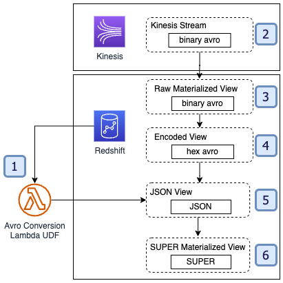
The basic architecture for this solution is as follows.

See the following code:
-- Step 1
CREATE OR REPLACE EXTERNAL FUNCTION fn_lambda_decode_avro_binary(varchar)
RETURNS varchar IMMUTABLE LAMBDA 'redshift-avro-udf';

-- Step 2
CREATE EXTERNAL SCHEMA kds FROM KINESIS

-- Step 3
CREATE MATERIALIZED VIEW {name} AUTO REFRESH YES AS
SELECT
    -- Step 4
   t.kinesis_data AS binary_avro,
   to_hex(binary_avro) AS hex_avro,
   -- Step 5
   fn_lambda_decode_avro_binary('{stream-name}', hex_avro) AS json_string,
   -- Step 6
   JSON_PARSE(json_string) AS super_data,
   t.sequence_number,
   t.refresh_time,
   t.approximate_arrival_timestamp,
   t.shard_id
FROM kds.{stream_name} AS t
Let’s explore each step in more detail.
Create the Lambda UDF
The overall goal is to develop a method that can accept the raw data as input and produce JSON-encoded data as an output. This aligns with the Amazon Redshift ability to natively process JSON into the SUPER data type. The specifics of the function depend on the serialization and streaming approach. For example, using the assumed schema approach with Avro format, your Lambda function may complete the following steps:
- Take in the stream name and hexadecimal-encoded data as inputs.
- Use the stream name to perform a lookup to identify the schema for the given stream name.
- Decode the hexadecimal data into binary format.
- Use the schema to deserialize the binary data into readable format.
- Re-serialize the data into JSON format.
The f_glue_schema_registry_avro_to_json AWS samples example illustrates the process of decoding Avro using the assumed schema approach using the AWS Glue Schema Registry in a Lambda UDF to retrieve and use Avro schemas by stream name. For other approaches (such as embedded schema ID), you should author your Lambda function to handle deserialization as defined by your serialization process and schema registry implementation. If your application depends on an external schema registry or table lookup to process the message schema, we recommend that you implement caching for schema lookups to help reduce the load on the external systems and reduce the average Lambda function invocation duration.
When creating the Lambda function, make sure you accommodate the Amazon Redshift input event format and ensure compliance with the expected Amazon Redshift event output format. For details, refer to Creating a scalar Lambda UDF.
After you create and test the Lambda function, you can define it as a UDF in Amazon Redshift. For effective integration within Amazon Redshift, designate this Lambda function UDF as IMMUTABLE. This classification supports incremental materialized view updates. This treats the Lambda function as idempotent and minimizes the Lambda function costs for the solution, because a message doesn’t need to be processed if it has been processed before.
Configure the baseline Kinesis data stream
Regardless of your messaging format or approach (embedded schema, assumed schema, and embedded schema ID), you begin with setting up the external schema for streaming ingestion from your messaging source into Amazon Redshift. For more information, refer to Streaming ingestion.
CREATE EXTERNAL SCHEMA kds FROM KINESIS

IAM_ROLE 'arn:aws:iam::0123456789:role/redshift-streaming-role';
Create the raw materialized view
Next, you define your raw materialized view. This view contains the raw message data from the streaming source in Amazon Redshift VARBYTE format.
Convert the VARBYTE data to VARCHAR format
External Lambda function UDFs don’t support VARBYTE as an input data type. Therefore, you must convert the raw VARBYTE data from the stream into VARCHAR format to pass to the Lambda function. The best way to do this in Amazon Redshift is using the TO_HEX built-in method. This converts the binary data into hexadecimal-encoded character data, which can be sent to the Lambda UDF.
Invoke the Lambda function to retrieve JSON data
After the UDF has been defined, we can invoke the UDF to convert our hexadecimal-encoded data into JSON-encoded VARCHAR data.
Use the JSON_PARSE method to convert the JSON data to SUPER data type
Finally, we can use the Amazon Redshift native JSON parsing methods like JSON_PARSE, JSON_EXTRACT_PATH_TEXT, and more to parse the JSON data into a format that we can use for analytics.
Considerations
Consider the following when using this strategy:
- Cost – Amazon Redshift invokes the Lambda function in batches to improve scalability and reduce the overall number of Lambda invocations. The cost of this solution depends on the number of messages in your stream, the frequency of the refresh, and the invocation time required to process the messages in a batch from Amazon Redshift. Using the IMMUTABLE UDF type in Amazon Redshift can also help minimize costs by utilizing the incremental refresh strategy for the materialized view.
- Permissions and network access – The AWS Identity and Access Management (IAM) role used for the Amazon Redshift UDF must have permissions to invoke the Lambda function, and you must deploy the Lambda function such that it has access to invoke its external dependencies (for example, you may need to deploy it in a VPC to access private resources like a schema registry).
- Monitoring – Use Lambda function logging and metrics to identify errors in deserialization, connection to the schema registry, and data processing. For details on monitoring the UDF Lambda function, refer to Embedding metrics within logs and Monitoring and troubleshooting Lambda functions.
Conclusion
In this post, we dove into different data formats and ingestion methods for a streaming use case. By exploring strategies for handling non-JSON data formats, we examined the use of Amazon Redshift streaming to seamlessly ingest, process, and analyze these formats in near-real time using materialized views.
Furthermore, we navigated through schema-per-stream, embedded schema, assumed schema, and embedded schema ID approaches, highlighting their merits and considerations. To bridge the gap between non-JSON formats and Amazon Redshift, we explored the creation of Lambda UDFs for data parsing and conversion. This approach offers a comprehensive means to integrate diverse data streams into Amazon Redshift for subsequent analysis.
As you navigate the ever-evolving landscape of data formats and analytics, we hope this exploration provides valuable guidance to derive meaningful insights from your data streams. We welcome any thoughts or questions in the comments section.
About the Authors
 M Mehrtens has been working in distributed systems engineering throughout their career, working as a Software Engineer, Architect, and Data Engineer. In the past, M has supported and built systems to process terrabytes of streaming data at low latency, run enterprise Machine Learning pipelines, and created systems to share data across teams seamlessly with varying data toolsets and software stacks. At AWS, they are a Sr. Solutions Architect supporting US Federal Financial customers.
Sindhu Achuthan is a Sr. Solutions Architect with Federal Financials at AWS. She works with customers to provide architectural guidance on analytics solutions using AWS Glue, Amazon EMR, Amazon Kinesis, and other services. Outside of work, she loves DIYs, to go on long trails, and yoga.

 M Mehrtens has been working in distributed systems engineering throughout their career, working as a Software Engineer, Architect, and Data Engineer. In the past, M has supported and built systems to process terrabytes of streaming data at low latency, run enterprise Machine Learning pipelines, and created systems to share data across teams seamlessly with varying data toolsets and software stacks. At AWS, they are a Sr. Solutions Architect supporting US Federal Financial customers.
 Sindhu Achuthan is a Sr. Solutions Architect with Federal Financials at AWS. She works with customers to provide architectural guidance on analytics solutions using AWS Glue, Amazon EMR, Amazon Kinesis, and other services. Outside of work, she loves DIYs, to go on long trails, and yoga.


![[after a minute] "Okay, I think I've got it, thanks. Can I--" "oOOOooOOooo!"](https://imgs.xkcd.com/comics/a_halloween_carol.png "[after a minute] \"Okay, I think I've got it, thanks. Can I--\" \"oOOOooOOooo!\"")