Post Syndicated from Explosm.net original https://explosm.net/comics/lunch-2
New Cyanide and Happiness Comic
Post Syndicated from Explosm.net original https://explosm.net/comics/lunch-2
New Cyanide and Happiness Comic
Post Syndicated from Michael Kammer original https://blog.zabbix.com/the-zabbix-advantage-for-business/26497/
CIOs and CITOs know all too well that a smoothly functioning network is the backbone of any business. Your network has to guarantee reliability, performance, and security. An unreliable network, by contrast, means damaged productivity, negative customer perceptions, and haphazard security. The solution is network monitoring, and in this post we’ll explore the reasons why Zabbix is the ideal monitoring solution for any business.
Network monitoring is a critical IT process where all networking components (as well as key performance indicators like CPU utilization and network bandwidth) are constantly monitored to improve performance and eliminate bottlenecks. It provides real-time information that network administrators need to determine whether a network is running optimally.
At Zabbix, we’re here to help you deliver for your customers, flawlessly and without interruptions. Our monitoring solution is 100% open source, available in over 20 languages, and able to collect an unlimited amount of data. Designed with enterprise requirements in mind, Zabbix provides a comprehensive, “single pane of glass” view of any size environment. Put simply, Zabbix allows you to monitor anything – from physical and virtual servers or containers to network infrastructure, applications, and cloud services.
What’s more, we offer a wide variety of additional professional services to go along with our solution, including:
Keep reading to find out more about the difference Zabbix can make for your business.
IT teams are under enormous pressure to have their networks functioning perfectly 100% of the time, and with good reason. It’s simply not possible to run a business with a malfunctioning network. Here are 5 key reasons why you need to make network monitoring a top priority, and why Zabbix is the right answer for all of them.
A network monitoring solution’s main reason for being is to show whether a device is working or not. Taking a proactive approach to maintaining a healthy network will keep tech support requests and downtime to an absolute minimum. Zabbix makes it easy to do so by automatically detecting problem states in your metric flow. Not only that, but our automated predictive functions can also help you react proactively. They do this by forecasting a value for early alerting and predicting the time left until you reach a problem threshold. Automation then allows you to remove additional inefficiencies.
Having complete visibility of all your hardware and software assets allows you to easily monitor the health of your network. Zabbix lets businesses access metrics, issues, reports, and maps with a single click, allowing you to:
By making it easy to monitor anything, Zabbix lets you know which parts of your network are being properly used, overused, or underused. This can help you uncover unnecessary costs that can be eliminated or identify a network component that needs upgrading.
Today’s IT teams need to meet strict regulatory and protection standards in increasingly complex networks. Zabbix can spot changes in normal system behavior and unusual data flow. It can then either leverage multiple messaging channels to notify your team about anomalies or simply resolve any issues automatically.
Zabbix has an extensive track record of making businesses more productive by saving network management time and lowering operating costs. Servers, for example, are machines that inevitably break down from time to time. Being able to quickly re-launch after a failure has occurred and minimizing the server downtime are vital. By making sure your team is aware of any and all current and impending issues, Zabbix can reduce downtime and increase the productivity and efficiency of your business.
Whatever field you’re in, there’s no substitute for consistent, problem-free service when it comes to gaining the trust and loyalty of customers. Zabbix has an extensive track record of helping clients in multiple industries achieve their goals.
A typical hospital relies on tens of thousands of connected devices. Manually checking each one for anomalies simply isn’t practical. Establishing a stable service level is a vital issue in most industries, but in healthcare it’s literally a matter of life and death. With Zabbix, hospital IT teams receive potentially life-saving alerts if anything is out of the ordinary.
What’s more, Zabbix can monitor progress toward expected outcomes, providing up-to-the-minute statistics on data errors or IT system failures. Issues, response times, and potential bottlenecks are displayed in easy-to-read graphs and charts. This allows hospital staff to follow up on the presence or absence of problems.
Financial institutions of all sizes rely on their networks to maintain connectivity and productivity. By processing millions of checks per minute and considering very complex dependencies between different elements of infrastructure, Zabbix allows banks to proactively detect and resolve network problems before they turn into major business disruptions.
Zabbix is also designed to seamlessly connect distributed architecture, including remote offices, branches, and even individual ATMs. Some of our financial industry clients previously used up to 20 different monitoring tools. Each alert sent hundreds of emails to different people, making it impossible to effectively monitor the environment. Naturally, they found Zabbix’s ability to monitor many thousands of devices and “single pane of glass” view to be a significant upgrade.
In an age of digital course materials and resources, schools and universities can’t operate without functioning IT infrastructures. Our clients in education typically have heterogeneous infrastructures with thousands of servers and clients. They also possess all kinds of connected devices, dozens of different operating systems, multiple locations, and hundreds of IT staff.
Zabbix has proven itself to be a simple, cost-effective method of monitoring geographically distributed campuses and educational sites. We’ve done this by:
Network monitoring is critical for government agencies, as downtime can bring a halt to vital public services. Our public-sector clients range from city-wide public transportation companies all the way up to entire prefectures. They use Zabbix to monitor the availability of utilities, transport, lighting, and many other public services.
In the process, Zabbix increases the effectiveness of budget expenditures by providing precise and accountable data on how public resources are used. This makes it easier to justify further expenditures. In most business software, agents are required for each monitored host and costs increase in proportion to the number of monitored hosts. By contrast, Zabbix is open source and the software itself is free of charge, resulting in anticipated cost reductions of up to 25% in many cases.
Retail environments increasingly depend on network-connected equipment, particularly when it comes to warehouse monitoring and tracking SKUs (stock keeping units). Zabbix delivers an all-in-one tool to monitor different applications, metrics, processes, and equipment while providing a complete picture about the availability and performance of all the components that make a retail business successful. This makes it possible for retailers to easily automate store openings and closings, monitor cash machines, and keep track of access system log entries.
Not only that, the quantity and quality of information that Zabbix collects makes it easy for retailers to conduct a more accurate analysis of what is happening (or what may happen) and take preventive measures. Our retail clients find that having this level of control over their resources and services increases the confidence of their teams as well as their customers.
Internet, telephony, and television verticals require availability and consistency. The key to success is providing your services 24/7/365.
Zabbix makes this possible by providing full visibility of all network and customer devices, allowing operators to know of any outage before customers do and take necessary actions. Some of our telecommunications clients are able to effortlessly monitor well over 100,000 devices with a single Zabbix server. This helps them improve the customer experience and driving growth in the process.
In the aerospace industry, timely data delivery and issue notification are the keys to safe operations. Aircraft depend on complex electronic systems that can diagnose the slightest deviations and make malfunctions known. Unfortunately, this is often in the form of either an indicator light on an instrument panel or a log message that is accessible only with specialized software or tools.
With Zabbix, all data transfers from the aircraft’s diagnostic system to the responsible employees can happen automatically. Error prioritization and escalation to further levels can also happen automatically if any aircraft has an ongoing issue that remains active for multiple days.
At Zabbix, our goal is a world without interruptions, powered by a world-class universal monitoring solution that’s available and affordable to any business. Our open-source software allows you to monitor your entire IT stack, no matter what size your infrastructure is or where it’s hosted.
That’s why government institutions across the globe as well as some of the world’s largest companies trust us with their network monitoring needs.
Get in touch with us to learn more and get started on the path to maximum efficiency and uptime today!
The post The Zabbix Advantage for Business appeared first on Zabbix Blog.
Post Syndicated from Matt Granger original https://www.youtube.com/watch?v=j7FASDFlfQo
Post Syndicated from xkcd.com original https://xkcd.com/2834/

Post Syndicated from Aarthi Srinivasan original https://aws.amazon.com/blogs/big-data/introducing-hybrid-access-mode-for-aws-glue-data-catalog-to-secure-access-using-aws-lake-formation-and-iam-and-amazon-s3-policies/
AWS Lake Formation helps you centrally govern, secure, and globally share data for analytics and machine learning. With Lake Formation, you can manage access control for your data lake data in Amazon Simple Storage Service (Amazon S3) and its metadata in AWS Glue Data Catalog in one place with familiar database-style features. You can use fine-grained data access control to verify that the right users have access to the right data down to the cell level of tables. Lake Formation also makes it simpler to share data internally across your organization and externally. Further, Lake Formation integrates with AWS analytics services such as Amazon Athena, Amazon Redshift Spectrum, Amazon EMR, and AWS Glue ETL for Apache Spark. These services allow querying Lake Formation managed tables, thus helping you extract business insights from the data quickly and securely.
Before the introduction of Lake Formation and its database-style permissions for data lakes, you had to manage access to your data in the data lake and its metadata separately through AWS Identity and Access Management (IAM) policies and S3 bucket policies. With an IAM and Amazon S3 access control mechanism, which is more complex and less granular compared to Lake Formation, you need more time to migrate to Lake Formation because a given database or table in the data lake could have its access controlled by either IAM and S3 policies or Lake Formation policies, but not both. Also, various use cases operate on the data lakes. Migrating all use cases from one permissions model to another in a single step without disruption was challenging for operations teams.
To ease the transition of data lake permissions from an IAM and S3 model to Lake Formation, we’re introducing a hybrid access mode for AWS Glue Data Catalog. Please refer to the What’s New and documentation. This feature lets you secure and access the cataloged data using both Lake Formation permissions and IAM and S3 permissions. Hybrid access mode allows data administrators to onboard Lake Formation permissions selectively and incrementally, focusing on one data lake use case at a time. For example, say you have an existing extract, transform and load (ETL) data pipeline that uses the IAM and S3 policies to manage data access. Now you want to allow your data analysts to explore or query the same data using Amazon Athena. You can grant access to the data analysts using Lake Formation permissions, to include fine-grained controls as needed, without changing access for your ETL data pipelines.
Hybrid access mode allows both permission models to exist for the same database and tables, providing greater flexibility in how you manage user access. While this feature opens two doors for a Data Catalog resource, an IAM user or role can access the resource using only one of the two permissions. After Lake Formation permission is enabled for an IAM principal, authorization is completely managed by Lake Formation and existing IAM and S3 policies are ignored. AWS CloudTrail logs provide the complete details of the Data Catalog resource access in Lake Formation logs and S3 access logs.
In this blog post, we walk you through the instructions to onboard Lake Formation permissions in hybrid access mode for selected users while the database is already accessible to other users through IAM and S3 permissions. We will review the instructions to set-up hybrid access mode within an AWS account and between two accounts.
In this scenario, we walk you through the steps to start adding users with Lake Formation permissions for a database in Data Catalog that’s accessed using IAM and S3 policy permissions. For our illustration, we use two personas: Data-Engineer, who has coarse grained permissions using an IAM policy and an S3 bucket policy to run an AWS Glue ETL job and Data-Analyst, whom we will onboard with fine grained Lake Formation permissions to query the database using Amazon Athena.
Scenario 1 is depicted in the diagram shown below, where the Data-Engineer role accesses the database hybridsalesdb using IAM and S3 permissions while Data-Analyst role will access the database using Lake Formation permissions.

To set up Lake Formation and IAM and S3 permissions for a Data Catalog database with Hybrid access mode, you must have the following prerequisites:
hybridsalesdb and has a set of eight tables, as shown in the following screenshot. You can use any of your datasets to follow along.
There are two personas that are IAM roles in the account: Data-Engineer and Data-Analyst. Their IAM policies and access are described as follows.
The following IAM policy on the Data-Engineer role allows access to the database and table metadata in the Data Catalog.
The following IAM policy on the Data-Engineer role grants data access to the underlying Amazon S3 location of the database and tables.
The Data-Engineer also has access to the AWS Glue console using the AWS managed policy arn:aws:iam::aws:policy/AWSGlueConsoleFullAccess and regressive iam:Passrole to run an AWS Glue ETL script as below.
The following policy is also added to the trust policy of the Data-Engineer role to allow AWS Glue to assume the role to run the ETL script on behalf of the role.
See AWS Glue studio set up for additional permissions required to run an AWS Glue ETL script.
The Data-Analyst role has the data lake basic user permissions as described in Assign permissions to Lake Formation users.
Additionally, the Data-Analyst has permissions to write Athena query results to an S3 bucket that isn’t managed by Lake Formation and Athena console full access using the AWS managed policy arn:aws:iam::aws:policy/AmazonAthenaFullAccess.
Complete the following steps to configure your data location in Amazon S3 with Lake Formation in hybrid access mode and grant access to the Data-Analyst role.


hybridsalesdb. You will select the database that has the data in the S3 location that you registered in the preceding step. From the Actions drop down menu, select Grant.
Data-Analyst for IAM users and roles. Under LF-Tags or catalog resources, select Named Data Catalog resources and select hybridsalesdb for Databases.

hybridsalesdb. Select Grant from the Actions drop down menu.Data-Analyst for IAM users and roles. Under LF-Tags or catalog resources, choose Named Data Catalog resources and select hybridsalesdb for Databases.hybridcustomer, hybridproduct, and hybridsales_order from the drop down.

Data-Analyst.
hybridsalesdb database and the three tables.
Data-Analyst.

Data-Engineer.catalog_id, database, and table_name to suit your sample.


Thus, you can add Lake Formation permissions to a new role to access a Data Catalog database without interfering with another role that is accessing the same database through IAM and S3 permissions.
This is a cross-account sharing scenario where a data producer shares a database and its tables to a consumer account. The producer provides full database access for an AWS Glue ETL workload on the consumer account. At the same time, the producer shares a few tables of the same database to the consumer account using Lake Formation. We walk you through how you can use hybrid access mode to support both access methods.

The producer account set up is similar to that of scenario 1 and we discuss the extra steps for scenario 2 in the following section.
The consumer Data-Engineer role is granted Amazon S3 data access using the producer’s S3 bucket policy and Data Catalog access using the producer’s Data Catalog resource policy.
The S3 bucket policy in the producer account follows:
The Data Catalog resource policy in the producer account is shown below. You also need the glue:ShareResource IAM permission for AWS Resource Access Manager (AWS RAM) to enable cross-account sharing.
PutDataLakeSettings() API. Choose the AWS Region where you have your sample data set in an S3 bucket and its corresponding database and tables in the Data Catalog.


The steps to share the database hybridsalesdb to the consumer account are similar to the steps to set up scenario 1.
hybridsalesdb. Select your database that has the data in the S3 location that you registered previously. From the Actions drop down menu, select Grant.


Note: Selecting the checkbox opts-in the consumer account Lake Formation administrator roles to use Lake Formation permissions without interrupting access to the consumer account’s IAM and S3 access for the same database.


You have now enabled cross-account sharing using Lake Formation permissions without revoking access to the IAMAllowedPrincipal virtual group.
In scenario 2, the Data-Analyst and Data-Engineer roles are created in the consumer account similar to scenario 1, but these roles access the database and tables shared from the producer account.
In addition to arn:aws:iam::aws:policy/AWSGlueConsoleFullAccess and arn:aws:iam::aws:policy/CloudWatchFullAccess, the Data-Engineer role also has permissions to create and run an Apache Spark job in AWS Glue Studio.
Data-Engineer has the following IAM policy that grants access to the producer account’s S3 bucket, which is registered with Lake Formation in hybrid access mode.
Data-Engineer has the following IAM policy that grants access to the consumer account’s entire Data Catalog and producer account’s database hybridsalesdb and its tables.
The Data-Analyst has the same IAM policies similar to scenario 1, granting basic data lake user permissions. For additional details, see Assign permissions to Lake Formation users.


hybridsalesdb and select Create resource link from the Actions drop down menu.
rl_hybridsalesdb as the name for the resource link and leave the rest of the selections as they are. Choose Create.
rl_hybridsalesdb. Select Grant from the Actions drop down menu.
Data-Analyst.
rl_hybridsalesdb from the Databases under Catalog in the left navigation bar. Select Grant on target from the Actions drop down menu.
Data-Analyst for IAM users and roles, keep the already selected database hybridsalesdb.

rl_hybridsalesdb from Databases under Catalog in the left navigation bar. Select Grant on target from the Actions drop down menu.Data-Analyst for IAM users and roles. Select All tables of the database hybridsalesdb. Select Select under Table permissions.

Data-Analyst.AWSDataDatalog for Data source. For Tables, select the three dots next to any of the table names. Select Preview Table to run the query.
Data-Engineer.You’ve added Lake Formation permissions to a new role Data-Analyst, without interrupting existing IAM and S3 access to Data-Engineer for a cross-account sharing use-case.
If you’ve used sample datasets from your S3 for this blog post, we recommend removing relevant Lake Formation permissions on your database for the Data-Analyst role and cross-account grants. You can also remove the hybrid access mode opt-in and remove the S3 bucket registration from Lake Formation. After removing all Lake Formation permissions from both the producer and consumer accounts, you can delete the Data-Analyst and Data-Engineer IAM roles.
Currently, only a Lake Formation administrator role can opt in other users to use Lake Formation permissions for a resource, since opting in user access using either Lake Formation or IAM and S3 permissions is an administrative task requiring full knowledge of your organizational data access setup. Further, you can grant permissions and opt in at the same time using only the named-resource method and not LF-Tags. If you’re using LF-Tags to grant permissions, we recommend you use the Hybrid access mode option on the left navigation bar to opt in (or the equivalent CreateLakeFormationOptin() API using the AWS SDK or AWS CLI) as a subsequent step after granting permissions.
In this blog post, we went through the steps to set up hybrid access mode for Data Catalog. You learned how to onboard users selectively to the Lake Formation permissions model. The users who had access through IAM and S3 permissions continued to have their access without interruptions. You can use Lake Formation to add fine-grained access to Data Catalog tables to enable your business analysts to query using Amazon Athena and Amazon Redshift Spectrum, while your data scientists can explore the same data using Amazon Sagemaker. Data engineers can continue to use their IAM and S3 permissions on the same data to run workloads using Amazon EMR and AWS Glue. Hybrid access mode for the Data Catalog enables a variety of analytical use-cases for your data without data duplication.
To get started, see the documentation for hybrid access mode. We encourage you to check out the feature and share your feedback in the comments section. We look forward to hearing from you.
 Aarthi Srinivasan is a Senior Big Data Architect with AWS Lake Formation. She likes building data lake solutions for AWS customers and partners. When not on the keyboard, she explores the latest science and technology trends and spends time with her family.
Post Syndicated from Patrick Kennedy original https://www.servethehome.com/the-end-of-another-sth-era-the-austin-texas-studio-is-in-shambles/
Today marks the end of another STH era as the Austin Texas studio went from production to shambles, to boxes en route to a better future
The post The End of Another STH Era The Austin Texas Studio is in Shambles appeared first on ServeTheHome.
Post Syndicated from Curious Droid original https://www.youtube.com/watch?v=2ySX3WzZuxk
Post Syndicated from James Beswick original https://aws.amazon.com/blogs/compute/visually-design-your-application-with-aws-application-composer/
This post is written by Paras Jain, Senior Technical Account Manager and Curtis Darst, Senior Solutions Architect.
AWS Application Composer allows you to design and build applications visually using 13 AWS CloudFormation resource types. Today, the service expands the support to all available CloudFormation resource types.
AWS Application Composer provides you with an interactive canvas for visually designing your applications. You use a drag-and-drop interface to create an application design from scratch or import an existing application definition to edit it.
Modern event-driven applications are built on many services. Visualizing an architecture helps you better understand the relationship between those services and identify gaps and areas of improvements.
You can use AWS Application Composer in local sync mode to connect to your local file system. That way your changes are updated to your file system. This way, you can integrate with existing version control systems and development and deployment workflow.
AWS Application Composer provides a drag-and-drop canvas view and a code editor template view. Changes made to one view reflect on the other view. Similarly, changes made in AWS Application Composer are reflected in your local code editor and vice versa.
AWS Application Composer already supports 13 serverless resource types. For these resource types, AWS Application Composer provides enhanced component cards.
Enhanced component cards allow you to configure and join components together. Today’s release gives you the ability to drag and drop 1,134 resource types to the canvas and configure these using resource configuration pane.
This blog post shows how you can create a fault tolerant compute architecture involving an Application Load Balancer, two Amazon Elastic Compute Cloud (EC2) instances in different Availability Zones, and an Amazon Relational Database Service (RDS) instance.
Conceptually, this is the application design:

For this blog post, you create a fault tolerant compute stack consisting of an ALB, two EC2 instances in two different Availability Zones with automatic scaling capabilities and an RDS instance.

Resources:
  DBEC2SecurityGroup:
    Type: AWS::EC2::SecurityGroup
    Properties:
      GroupDescription: Open database for access
      SecurityGroupIngress:
        - IpProtocol: tcp
          FromPort: '3306'
          ToPort: '3306'
          SourceSecurityGroupId: !Ref WebServerSecurityGroup
      VpcId:
        ParameterId: VpcId
        Format: AWS::EC2::VPC::Id
  WebServerSecurityGroup:
    Type: AWS::EC2::SecurityGroup
    Properties:
      GroupDescription: Enable HTTP access via port 80 locked down to the load balancer + SSH access.
      SecurityGroupIngress:
        - IpProtocol: tcp
          FromPort: '80'
          ToPort: '80'
          SourceSecurityGroupId: !Select
            - 0
            - !GetAtt LoadBalancer.SecurityGroups
        - IpProtocol: tcp
          FromPort: '22'
          ToPort: '22'
          CidrIp:
            ParameterId: SSHLocation
            Format: String
            Default: 0.0.0.0/0
      VpcId:
        ParameterId: VpcId
        Format: AWS::EC2::VPC::Id
  WebServerGroup:
    Type: AWS::AutoScaling::AutoScalingGroup
    Properties:
      VPCZoneIdentifier:
        ParameterId: Subnets
        Format: List<AWS::EC2::Subnet::Id>
      LaunchConfigurationName: !Ref LaunchConfiguration
      MinSize: '1'
      MaxSize: '5'
      DesiredCapacity:
        ParameterId: WebServerCapacity
        Format: Number
        Default: '1'
      TargetGroupARNs:
        - !Ref TargetGroup


DefaultActions:
     Type: forward
TargetGroupArn: !Ref TargetGroup
LoadBalancerArn: !Ref LoadBalancer
Port: '80'
Protocol: HTTPHealthCheckPath: /
HealthCheckIntervalSeconds: 10
HealthCheckTimeoutSeconds: 5
HealthyThresholdCount: 2
Port: 80
Protocol: HTTP
UnhealthyThresholdCount: 5
VpcId:
ParameterId: VpcId
Format: AWS::EC2::VPC::Id
TargetGroupAttributes:
- Key: stickiness.enabled
Value: 'true'
- Key: stickiness.type
Value: lb_cookie
- Key: stickiness.lb_cookie.duration_seconds
Value: '30'
ImageId: <image-id>
InstanceType: t2.small
SecurityGroups: !Ref WebServerSecurityGroup
DBName:
  ParameterId: DBName
  Format: String
  Default: wordpressdb
Engine: MySQL
MultiAZ:
  ParameterId: MultiAZDatabase
  Format: String
  Default: 'false'
MasterUsername:
  ParameterId: DBUser
  Format: String
MasterUserPassword:
  ParameterId: DBPassword
  Format: String
DBInstanceClass:
  ParameterId: DBClass
  Format: String
  Default: db.t2.small
AllocatedStorage:
  ParameterId: DBAllocatedStorage
  Format: Number
  Default: '5'
VPCSecurityGroups:
  - !GetAtt DBEC2SecurityGroup.GroupId

After adding the core application components, you now add observability to your application. Observability enables you to collect and analyze important events and metrics for your applications.
To be notified of any changes to the RDS database configuration, use a serverless design pattern to avoid running instances when they are not needed. Conceptually, your observability stack looks like:

There are now two distinct sets of components in the architecture. One set of components comprises the core application while another comprises the observability logic.
AWS Application Composer allows you to organize different components in groups. This allows you and your team to focus on one portion of the architecture at a time. Before adding observability components, first create a group of the existing components.

Once the group is created, follow these steps to rename the group.

Now add the observability components. Repeat the process of searching then dragging and dropping of the following components from the Resources pane to the canvas outside the Application Stack group.
Repeat the process for grouping these 4 components in a group with the name Observability.
Some of the components have a small circle on their sides. These are connector ports. A port on the right side of a card indicates an opportunity for the card to invoke another card. A port on the left side indicates an opportunity for a card to be invoked by another card. You can connect two cards by clicking the right port of a card and dragging to the left port of another card.
Create the observability stack by following the following steps:
source:
  - aws.rds
detail-type:
  - RDS DB Instance Event
    Endpoint: [email protected]
    Protocol: email
    TopicArn: !Ref Topic

Before you can provision the resources for your architecture, you must make the configuration changes as per development and deployment best practices for your organization.
For example, you must provide a strong DB password, name the resources as per the naming conventions of your organization. You must also add the Lambda code with your custom logic.
AWS Application Composer provides you the ability to configure each resource via resource configuration panel. This enables you to always stay in-context while creating a complex architecture. You can quickly find the resource you want to edit instead of scrolling through a large template file. If you prefer to edit the template file directly, you can use the Template View of AWS Application Composer.
Alternatively, if you have enabled the local sync, you can edit the file directly in your integrated development environment (IDE) where changes made in AWS Application Composer are saved in real-time. If you have not enabled the local sync, you can export the template using the Save Template File option in the menu. After concluding your changes, you can provision the AWS infrastructure either by using AWS CloudFormation Console or by command line interface.
AWS Application Composer does not provision any AWS resources. Using AWS Application Composer to design your application architecture is free. You are only charged when you provision AWS Resources using the template file created by AWS Application Composer.
This blog post shows how to use AWS Application Composer to create and update an application architecture using any of the 1,134 CloudFormation resource types. It covers how to configure local sync mode to integrate the AWS Application to your development workflow. The post demonstrates how to organize your architecture into two distinct groups. Changes made in Canvas view are reflected in the template view and vice versa.
To learn more about AWS Application Composer visit https://aws.amazon.com/application-composer/.
For more serverless learning resources, visit Serverless Land.
Post Syndicated from Harith Gaddamanugu original https://aws.amazon.com/blogs/security/deploy-aws-managed-rules-using-security-automations-for-aws-waf/
You can now deploy AWS WAF managed rules as part of the Security Automations for AWS WAF solution. In this post, we show you how to get started and set up monitoring for this automated solution with additional recommendations.
This article discusses AWS WAF, a service that assists you in protecting against typical web attacks and bots that might disrupt availability, compromise security, or consume excessive resources. As requests for your websites are received by the underlying service, they’re forwarded to AWS WAF for inspection against your rules. AWS WAF informs the underlying service to either block, allow, or take another configured action when a request fulfills the criteria stated in your rules. AWS WAF is tightly integrated with Amazon CloudFront, Application Load Balancer (ALB), Amazon API Gateway, and AWS AppSync—all of which are routinely used by AWS customers to provide content for their websites and applications.
To provide a simple, purpose-driven deployment approach, our solutions builder teams developed Security Automations for AWS WAF, a solution that can help organizations that don’t have dedicated security teams to quickly deploy an AWS WAF that filters common web-based malicious activity. Security Automations for AWS WAF deploys a set of preconfigured rules to help you protect your applications from common web exploits.
This solution can be installed in your AWS accounts by launching the provided AWS CloudFormation template.
Security Automations for AWS WAF provides the following features and benefits:

Figure 1: Design overview of the new Security Automations for AWS WAF solution
Many customers begin their proofs of concept (POC) by using the AWS Management Console for AWS WAF to set up their very first AWS WAF, but quickly realize the benefits of automation, such as increased productivity, enforcing best practices, avoiding repetition, and so on. Manually managing AWS WAF can be time-consuming, especially if you want to duplicate complicated automations across multiple environments.
You can deploy this solution for new and existing supported AWS WAF resources. The implementation guide discusses architectural considerations, configuration steps, and operational best practices for deploying this solution in the AWS Cloud. It includes links to AWS CloudFormation templates and stacks that launch, configure, and run the AWS security, compute, storage, and other services required to deploy this solution on AWS, using AWS best practices for security and availability.
Before you launch the CloudFormation template, review the architecture and configuration considerations discussed in this guide. The template takes about 15 minutes to deploy and includes three basic steps:
Associate your CloudFront web distributions or ALBs with the web ACL that this solution generates. You can associate as many distributions or load balancers as you want.
Turn on web access logging for your CloudFront web distributions or ALBs, and send the log files to the appropriate Amazon Simple Storage Service (Amazon S3) bucket. Save the logs in a folder matching the user-defined prefix. If no user-defined prefix is used, save the logs to AWSLogs (default log prefix AWSLogs/).
This solution provides an example of how to use AWS WAF and other services to build security automations on the AWS Cloud. You can download the open source code from GitHub to apply customizations or build your own security automations that fit your needs. The solution builder team is planning to release a Terraform version for this solution in the near future.
This solution includes a Service Catalog AppRegistry resource to register the CloudFormation template and underlying resources as an application in both the Service Catalog AppRegistry and Systems Manager Application Manager. You can monitor the costs and operations data in the Systems Manager console, as shown in Figure 2 that follows.

Figure 2: Example of the application view for the Security Automations for AWS WAF stack in Application Manager
CloudWatch dashboards are customizable home pages in the CloudWatch console that you can use to monitor your resources in a single view, including visualizing AWS WAF logs as shown in Figure 3 that follows. The solution creates a simple dashboard that you can customize to monitor additional metrics, alarms and logs. If suspicious activity is reported, you can use the visuals to understand the traffic in more detail and drive incident response actions as needed. From here, you can investigate further by using specific queries with CloudWatch Logs Insights.

Figure 3: Example of an enhanced AWS WAF CloudWatch dashboard that can be built for monitoring your site traffic
In this post, you learned about using the AWS Security Automation template to quickly deploy AWS WAF. If you prefer a simpler solution, we recommend using the one-click CloudFront AWS WAF setup, which offers a simple way to deploy AWS WAF for your CloudFront distribution. By choosing the approach that aligns with your requirements, you can enhance the security of your web applications and safeguard them against potential threats.
For more solutions, visit the AWS Solutions Library.
If you have feedback about this post, submit comments in the Comments section below. If you have questions about this post, contact AWS Support.
Want more AWS Security news? Follow us on Twitter.
Post Syndicated from jake original https://lwn.net/Articles/945504/
The AI boom is clearly upon us, but there are still plenty of questions
swirling around this technology. Some of those questions are legal ones
and there have been lawsuits filed to try to get clarification—and perhaps
monetary damages. Van Lindberg is a lawyer who is well-known in the
open-source world; he came to Open
Source Summit Europe 2023 in Bilbao, Spain to try to put the current
work in AI into its legal context.
Post Syndicated from Max Wagner original https://github.blog/2023-09-26-how-github-uses-github-actions-and-actions-larger-runners-to-build-and-test-github-com/
The Developer Experience (DX) team at GitHub collaborated with a number of other teams to work on moving our continuous integration (CI) system to GitHub Actions to support the development and scaling demands of our engineering team. Our goal as a team is to enable our engineers to confidently and quickly ship software. To that end, we’ve worked on providing paved paths, a suite of automated tools and applications to streamline our development, runtime platforms, and deployments. Recently, we’ve been working to make our CI experience better by leveraging the newly released GitHub feature, Actions larger runners, to run our CI.
Read on to see how we run 15,000 CI jobs within an hour across 150,000 cores of compute!
GitHub has invested in a variety of different CI systems throughout its history. With each system, our aim has been to enhance the development experience for both GitHub engineers writing and deploying code and for engineers maintaining the systems.
However, with past CI systems we faced challenges with scaling the system to meet the needs of our engineering team to provide both stable and ephemeral build environments. Neither of these challenges allowed us to provide the optimal developer experience.
Then, GitHub released GitHub Actions larger runners. This gave us an opportunity not only to transition to a fully featured CI system, but also to develop, experience, and utilize the systems we are creating for our customers and to drive feedback to help build the product. For the GitHub DX team, this transition was a great opportunity to move away from maintaining our past CI systems while delivering a superior developer experience.
Larger runners are GitHub Actions runners that are hosted by GitHub. They are managed virtual machines (VMs) with more RAM, CPU, and disk space than standard GitHub-hosted runners. There are a variety of different machine sizes offered for the runners as well as some additional features compared to the standard GitHub-hosted runners.
Larger runners are available to GitHub Team and GitHub Enterprise Cloud customers. Check out these docs to learn more about larger runners.
Coming from previous iterations of GitHub’s CI systems, we needed the ability to create CI machines on demand to meet the fast feedback cycles needed by GitHub engineers and to scale with the rate of change of the site.
With larger runners, we maintain the ability to autoscale our CI system because GitHub will automatically create multiple instances of a runner that scale up and down to match the job demands of our engineers. An added benefit is that the GitHub DX team no longer has to worry about the scaling of the runners since all of those complexities are handled by GitHub itself!
We wanted to share some raw numbers on our current peak utilization of larger runners:
GitHub Actions provides runners with a lot of tools already baked in, which is sufficient and convenient for a variety of projects across the company. However, for some complex production GitHub services, the prebuilt runners did not satisfy all our requirements.
To maintain an efficient and fast CI system, the DX team needed the ability to provide machines with all the tools needed to build those production services. We didn’t want to spend extra time installing tools or compiling projects during CI jobs.
We are currently building features into larger runners so they have the ability to be launched from a custom VM image, called custom images. While this feature is still in beta, using custom images is a huge benefit to GitHub’s CI lifecycle for a couple of reasons.
First, custom images allows GitHub to bundle all the required software and tools needed to build and test complex production bearing services. Anything that is unique to GitHub or one of our projects can be pre-installed on the image before a GitHub Actions workflow even starts.
Second, custom images enable GitHub to dramatically speed up our GitHub Actions workflows by acting as a bootstrapping cache for some projects. During custom image creation, we bundle a pre-built version of a project’s source code into the image. Subsequently, when the project starts a GitHub Actions workflow, it can utilize a cached version of its source code, and any other build artifacts, to speed up its build process.
The cached project source code on the custom VM image can quickly become out of date due to the rapid rate of development within GitHub. This, in turn, causes workflow durations to increase. The DX team worked with the GitHub Actions engineering team to create an API on GitHub to regularly update the custom image multiple times a day to keep the project source up to date.
In practice, this has reduced the bootstrapping time of our projects significantly. Without custom images, our workflows would take around 50 minutes from start to finish, versus the 12 minutes they take today. This is a game changer for our engineers.
We’re working on a way to offer this functionality at scale. If you are interested in custom images for your CI/CD workflows, please reach out to your account manager to learn more!
There are thousands of projects at GitHub — from services that run production workloads to small tools that need to run CI to perform their daily operations. To make this a reality, GitHub leverages several important features in GitHub Actions that enable us to use the platform efficiently and securely across the company at scale.
One of the DX team’s driving goals is to pave paths for all repositories to run CI without introducing unnecessary repetition across repositories. Prior to GitHub Actions, we created single job configurations that could be used across multiple projects. In GitHub Actions, this was not as easy because any repository can define its own workflows. Reusable workflows to the rescue!
The reusable workflows feature in GitHub Actions provides a way to centrally manage a workflow in a repository that can be utilized by many other repositories in an organization. This was critical in our transition from our previous CI system to GitHub Actions. We were able to create several prebuilt workflows in a single repository, and many repositories could then use those workflows. This makes the process of adding CI to an existing or new project very much plug and play.
In our central repository hosting our reusable workflows, we can have workflows defined like:
on:
  workflow_call:
    inputs:
      cibuild-script:
        description: 'Which cibuild script to run.'
        type: string
        required: false
        default: "script/cibuild"
    secrets:
      service-api-key:
        required: true

jobs:
  reusable_workflow_job:
    runs-on: gh-larger-runner-medium
    name: Simple Workflow Job
    timeout-minutes: 20
    steps:
      - name: Checkout Project
        uses: actions/checkout@v3
      - name: Run cibuild script
        run: |
          bash ${{ inputs.cibuild-script }}
        shell: bash
And in consuming repositories, they can simply utilize the reusable workflow, with just a few lines of code!
name: my-new-project
on:
  workflow_dispatch:
  push:

jobs:
  call-reusable-workflow:
    uses: github/internal-actions/.github/workflows/default.yml@main
    with:
      cibuild-script: "script/cibuild-my-tests"
    secrets:
      service-api-key: ${{ secrets.SERVICE_API_KEY }}
Another great benefit of the reusable workflows feature is that the runner can be defined in the Reusable Workflow, meaning that we can guarantee all users of the workflow will run on our designated larger runner pool. Now, projects don’t need to worry about which runner they need to use!
To optimize our developer experience, the DX team worked with our engineering team to create a feature for GitHub Actions that allows workflows to reuse the outcome of a previous workflow run where the outcomes would be the same.
In some cases, the file contents of a repository are exactly the same between workflow runs that run on different commits. That is, the Git tree IDs for the current commit is the same as the previous commit (there are no file differences). In these cases, we can bypass CI checks by reusing the previous workflow outcomes and allow engineers to not have to wait for CI to run again.
This feature saves GitHub engineers from running anywhere from 300 to 500 workflows runs a day!
During some internal GitHub Actions workflow runs, the workflows need the ability to access some GitHub private services, within a GitHub virtual private cloud (VPC), over the network. These could be resources such as artifact storage, application metadata services, and other services that enable invocation of our test harness.
When we moved to larger runners, this requirement to access private services became a top-of-mind concern. In previous iterations of our CI infrastructure, these private services were accessible through other cloud and network configurations. However, larger runners are isolated from other production environments, meaning they cannot access our private services.
Like all companies, we need to focus on both the security of our platform as well as the developer experience. To satisfy these two requirements, GitHub developed a remote access solution that allows clients residing outside of our VPCs (larger runners) to securely access select private services.
This remote access solution works on the principle of minting an OIDC token in GitHub Actions, passing the OIDC token to a remote access gateway that authorizes the request by validating the OIDC token, and then proxying the request to the private service residing in a private network.
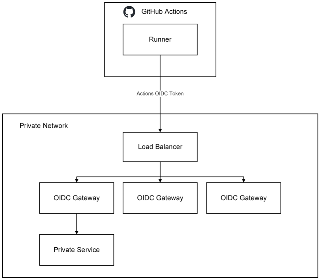
With this solution we are able to securely provide remote access from larger runners running GitHubActions to our private resources within our VPC.
GitHub has open sourced the basic scaffolding of this remote access gateway in the github/actions-oidc-gateway-example repository, so be sure to check it out!
GitHub Actions provides a robust and smooth developer experience for GitHub engineers working on GitHub.com. We have been able to accomplish this by using the power of GitHub Actions features, such as reusable workflows and reusable workflow outcomes, and by leveraging the scalability and manageability of the GitHub Actions larger runners. We have also used this effort to enhance the GitHub Actions product. To put it simply, GitHub runs on GitHub.
The post How GitHub uses GitHub Actions and Actions larger runners to build and test GitHub.com appeared first on The GitHub Blog.
Post Syndicated from Omar Gonzalez original https://aws.amazon.com/blogs/big-data/using-experian-identity-resolution-with-aws-clean-rooms-to-achieve-higher-audience-activation-match-rates/
This is a guest post co-written with Tyler Middleton, Experian Senior Partner Marketing Manager, and Jay Rakhe, Experian Group Product Manager.
As the data privacy landscape continues to evolve, companies are increasingly seeking ways to collect and manage data while protecting privacy and intellectual property. First party data is more important than ever for companies to understand their customers and improve how they interact with them, such as in digital advertising across channels. Companies are challenged with having a complete view of their customers as they engage with them across different channels and devices, in addition to other third parties that could complement their data to generate rich insights about their customers. This has driven companies to build identity graph solutions or use well-known identity resolution from providers such as Experian. It has also driven companies to grow their first-party consumer-consented data and collaborate with other companies and partners to create better-informed advertising campaigns.
AWS Clean Rooms allows companies to collaborate securely with their partners on their collective datasets without sharing or copying one another’s underlying data. Combining Experian’s identity resolution with AWS Clean Rooms can help you achieve higher match rates with your partners on your collective datasets when you run an AWS Clean Rooms collaboration. You can achieve higher match rates by using Experian’s diverse offline and digital ID database.
In this post, we walk through an example of a retail advertiser collaborating with a connected television (CTV) provider, facilitated by AWS Clean Rooms and Experian. AWS Clean Rooms facilitates a secure collaboration for an audience activation use case.
Retail advertisers recognize the growing consumer behaviors to use streaming TV services over traditional TV channels. Because of this, you may want to use your customer tiering and past purchase history datasets to target your audience in CTV.
The following example advertiser dataset includes the audience to be targeted on the CTV platform.
|
Advertiser ID |
First | Last | Address | City | State | Zip | Customer Tier | LTV | Last Purchase Date |
| 123 | Tyler | Smith | 4128 Et Street | Franklin | OK | 82736 | Gold | $823 | 8/1/21 |
| 456 | Karleigh | Jones | 2588 Nibh Street | Clinton | RI | 38947 | Gold | $741 | 2/2/22 |
| 984 | Alex | Brown | 6556 Tincidunt Avenue | Madison | WI | 10975 | Silver | $231 | 1/17/22 |
The following sample CTV provider dataset has email addresses and subscription status.
| Email Address | Status |
| [email protected] | Subscribed |
| [email protected] | Free Ad Tier |
| [email protected] | Trial |
Experian performs identity resolution on each dataset by matching against Experian’s attributes on 250 million consumers and 126 million households. Experian assigns a unique and synthetic Experian ID referred to as a Living Unit ID (LUID) to each matched record.
The Experian LUIDs for an advertiser and CTV provider are unique per consumer record. For example, LU_ADV_123 in the advertiser table corresponds to LU_CTV_135 in the CTV table. To allow the CTV provider and advertiser to match identities across the datasets, Experian generates a collaboration LUID, as shown in the following figure. This allows a double-blind join to be performed against both tables in AWS Clean Rooms.

The following figure illustrates the workflow in our example AWS Clean Rooms collaboration.
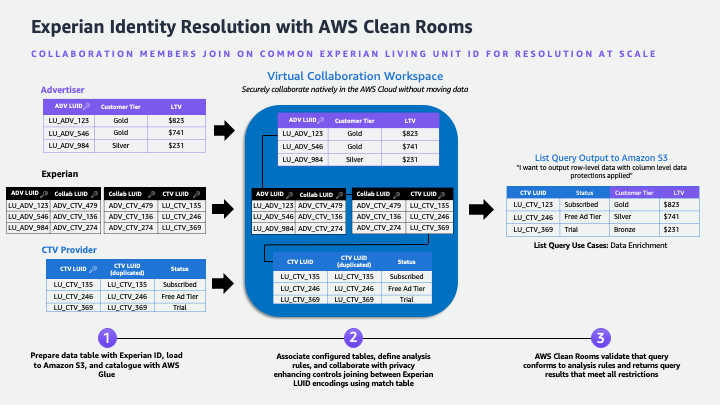
We walk you through the following high-level steps:
First, the advertiser and CTV provider engage with Experian directly to assign Experian LUIDs to their consumer records. During this process, both parties provide identity components to Experian as an input. Experian processes their input data and returns an Experian LUID when a matched identity is found. New and existing Experian customers can start this process by reaching out to Experian Marketing Services.
After the tables are prepared with Experian LUIDs, the advertiser, CTV provider, and Experian join an AWS Clean Rooms collaboration. A collaboration is a secure logical boundary in AWS Clean Rooms in which members perform SQL queries on configured tables. Any participant can create an AWS Clean Rooms collaboration. In this example, the CTV provider has created a collaboration in AWS Clean Rooms and invited the advertiser and Experian to join and contribute data, without sharing their underlying data with each other. The advertiser and Experian will log in to each of their respective AWS accounts and join the collaboration as a member.
The next step is to upload and catalog the data to be queried in AWS Clean Rooms. Each collaborator will upload their dataset to Amazon S3 object storage in their respective accounts. Next, the data is cataloged in the AWS Glue Data Catalog.
After the table is cataloged in the AWS Glue Data Catalog, it can be associated with an AWS Clean Rooms configured table. A configured table defines which columns can be used in the collaboration and contains an analysis rule that determines how the data can be queried.
In this step, Experian adds two configured tables that include the collaboration LUIDs that allow the CTV provider and advertiser to match across their datasets.
The advertiser has defined a list analysis rule that allows the CTV provider to run queries that return a row-level list of the collective data. They have also configured their unique Experian advertiser LUIDs as the join keys. In AWS Clean Rooms, join key columns can be used to join datasets, but the values can’t be returned in the result.
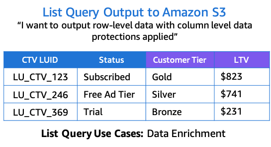
The CTV provider can now perform a SQL query against the datasets using the AWS Clean Rooms console or the AWS Clean Rooms StartProtectedQuery API.
The following sample list query returns the customer tier and LTV (lifetime value) for matched CTV identities:
The following figure illustrates the results.
In this post, we showed how a retail advertiser can enrich their data with CTV provider data using Experian in an AWS Clean Rooms collaboration, without sharing or exposing raw data with each other. The advertiser can now use the CTV customer tiering and subscription data to activate specific segments on the CTV platform. For example, if the retail advertiser wants to offer membership to their loyalty program, they can now target their high LTV customers that have a CTV paid subscription. With AWS Clean Rooms, this use case can be expanded further to include additional collaborators to further enrich your data. AWS Clean Rooms partners include identity resolution providers, such as Experian, who can help you more easily join data using Experian identifiers. To learn more about the benefits of Experian identity resolution, refer to Identity resolution solutions. New and existing customers can contact Experian Marketing Services to authorize an AWS Clean Rooms collaboration. Visit the AWS Clean Rooms User Guide to get started using AWS Clean Rooms today.
 Omar Gonzalez is a Senior Solutions Architect at Amazon Web Services in Southern California with more than 20 years of experience in IT. He is passionate about helping customers drive business value through the use of technology. Outside of work, he enjoys hiking and spending quality time with his family.
 Matt Miller is a Business Development Principal at AWS. In his role, Matt drives customer and partner adoption for the AWS Clean Rooms service specializing in advertising and marketing industry use cases. Matt believes in the primacy of privacy enhanced data collaboration and interoperability underpinning data-driven marketing imperatives from customer experience to addressable advertising. Prior to AWS, Matt led strategy and go-to market efforts for ad technologies, large agencies, and consumer data products purpose-built to inform smarter marketing and deliver better customer experiences.
Post Syndicated from Technology Connextras original https://www.youtube.com/watch?v=pmKL3pgPQhY
Post Syndicated from Talks at Google original https://www.youtube.com/watch?v=34UbISWn2m4
Post Syndicated from Olivier Gaumond original https://aws.amazon.com/blogs/security/enable-external-pipeline-deployments-to-aws-cloud-by-using-iam-roles-anywhere/
Continuous integration and continuous delivery (CI/CD) services help customers automate deployments of infrastructure as code and software within the cloud. Common native Amazon Web Services (AWS) CI/CD services include AWS CodePipeline, AWS CodeBuild, and AWS CodeDeploy. You can also use third-party CI/CD services hosted outside the AWS Cloud, such as Jenkins, GitLab, and Azure DevOps, to deploy code within the AWS Cloud through temporary security credentials use.
Security credentials allow identities (for example, IAM role or IAM user) to verify who they are and the permissions they have to interact with another resource. The AWS Identity and Access Management (IAM) service authentication and authorization process requires identities to present valid security credentials to interact with another AWS resource.
According to AWS security best practices, where possible, we recommend relying on temporary credentials instead of creating long-term credentials such as access keys. Temporary security credentials, also referred to as short-term credentials, can help limit the impact of inadvertently exposed credentials because they have a limited lifespan and don’t require periodic rotation or revocation. After temporary security credentials expire, AWS will no longer approve authentication and authorization requests made with these credentials.
In this blog post, we’ll walk you through the steps on how to obtain AWS temporary credentials for your external CI/CD pipelines by using IAM Roles Anywhere and an on-premises hosted server running Azure DevOps Services.
When you run code on AWS compute services, such as AWS Lambda, AWS provides temporary credentials to your workloads. In hybrid information technology environments, when you want to authenticate with AWS services from outside of the cloud, your external services need AWS credentials.
IAM Roles Anywhere provides a secure way for your workloads — such as servers, containers, and applications running outside of AWS — to request and obtain temporary AWS credentials by using private certificates. You can use IAM Roles Anywhere to enable your applications that run outside of AWS to obtain temporary AWS credentials, helping you eliminate the need to manage long-term credentials or complex temporary credential solutions for workloads running outside of AWS.
To use IAM Roles Anywhere, your workloads require an X.509 certificate, issued by your private certificate authority (CA), to request temporary security credentials from the AWS Cloud.
IAM Roles Anywhere can work with your existing client or server certificates that you issue to your workloads today. In this blog post, our objective is to show how you can use X.509 certificates issued by your public key infrastructure (PKI) solution to gain access to AWS resources by using IAM Roles Anywhere. Here we don’t cover PKI solutions options, and we assume that you have your own PKI solution for certificate generation. In this post, we demonstrate the IAM Roles Anywhere setup with a self-signed certificate for the purpose of the demo running in a test environment.
CI/CD services are typically composed of a control plane and user interface. They are used to automate the configuration, orchestration, and deployment of infrastructure code or software. The code build steps are handled by a build agent that can be hosted on a virtual machine or container running on-premises or in the cloud. Build agents are responsible for completing the jobs defined by a CI/CD pipeline.
For this use case, you have an on-premises CI/CD pipeline that uses AWS CloudFormation to deploy resources within a target AWS account. The CloudFormation template, the pipeline definition, and other files are hosted in a Git repository. The on-premises build agent requires permissions to deploy code through AWS CloudFormation within an AWS account. To make calls to AWS APIs, the build agent needs to obtain AWS credentials from an IAM role. The solution architecture is shown in Figure 1.
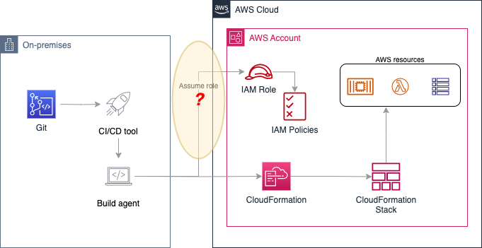
Figure 1: Using external CI/CD tool with AWS
To make this deployment securely, the main objective is to use short-term credentials and avoid the need to generate and store long-term credentials for your pipelines. This post walks through how to use IAM Roles Anywhere and certificate-based authentication with Azure DevOps build agents. The walkthrough will use Azure DevOps Services with Microsoft-hosted agents. This approach can be used with a self-hosted agent or Azure DevOps Server.
IAM Roles Anywhere uses a private certificate authority (CA) for the temporary security credential issuance process. Your private CA is registered with IAM Roles Anywhere through a service-to-service trust. Once the trust is established, you create an IAM role with an IAM policy that can be assumed by your services running outside of AWS. The external service uses a private CA issued X.509 certificate to request temporary AWS credentials from IAM Roles Anywhere and then assumes the IAM role with permission to finish the authentication process, as shown in Figure 2.
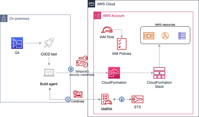
Figure 2: Certificate-based authentication for external CI/CD tool using IAM Roles Anywhere
The workflow in Figure 2 is as follows:
In this walkthrough, you accomplish the following steps:
You can find the sample code for this post in our GitHub repository. We recommend that you locally clone a copy of this repository. This repository includes the following files:
The first step is creating an IAM role in your AWS accounts with the necessary permissions to deploy your resources. For this, you create a role using the AWSCloudFormationFullAccess and AmazonDynamoDBFullAccess managed policies.
When you define the permissions for your actual applications and workloads, make sure to adjust the permissions to meet your specific needs based on the principle of least privilege.
Run the following command to create the CICDRole in the Dev and Prod AWS accounts.
As part of the role creation, you need to apply the trust policy provided in iamra-trust-policy.json. This trust policy allows the IAM Roles Anywhere service to assume the role with the condition that the Subject Common Name (CN) of the certificate is cicdagent.example.com. In a later step you will update this trust policy with the Amazon Resource Name (ARN) of your trust anchor to further restrict how the role can be assumed.
Use OpenSSL to generate and sign the certificate. Run the following commands to generate a root and leaf certificate.
Note: The following procedure has been tested with OpenSSL 1.1.1 and OpenSSL 3.0.8.
The following files are needed in further steps: ca.crt, certificate.crt, private.key.
In this step, you configure the IAM Roles Anywhere trust anchor, the profile, and the role with the associated IAM policy to define the permissions to be granted to your build agents. Make sure to set the permissions specified in the policy to the least privileged access.
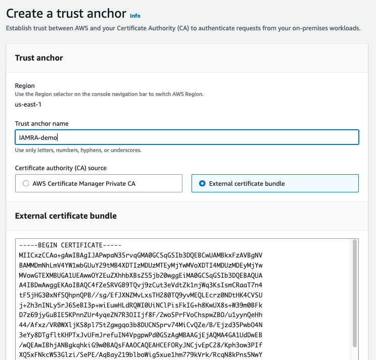
Figure 3: IAM Roles Anywhere trust anchor
To follow security best practices by applying least privilege access, add a condition statement in the IAM role’s trust policy to match the created trust anchor to make sure that only certificates that you want to assume a role through IAM Roles Anywhere can do so.
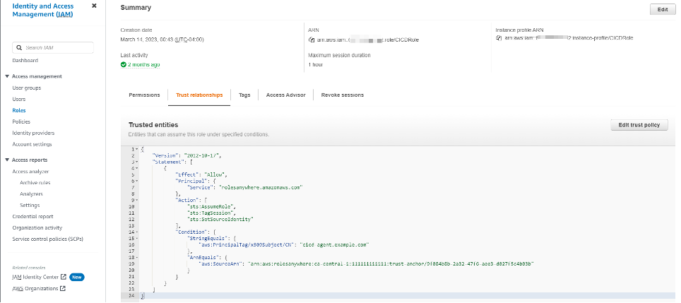
Figure 4: IAM Roles Anywhere updated trust policy
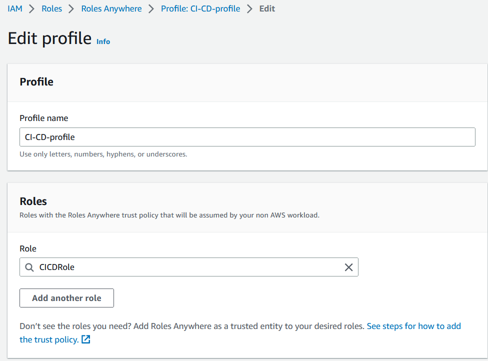
Figure 5: IAM Roles Anywhere profile
Now that you’ve completed the necessary setup in AWS, you move to the configuration of your pipeline in Azure DevOps. You need to have access to an Azure DevOps organization to complete these steps.
Have the following values ready. They’re needed for the Azure DevOps Pipeline configuration. You need this set of information for every AWS account you want to deploy to.
The following steps walk you through configuring Azure DevOps.

Figure 6: Azure DevOps configuration steps: Adding IAM Roles Anywhere variables

Figure 7: Azure DevOps configuration steps: Pipeline permissions

Figure 8: Azure DevOps configuration steps: Upload certificate and private key

Figure 9: Azure DevOps configuration steps: Pipeline permissions for each file

Figure 10: Verify CloudFormation stack deployment in your account
Here are the different steps of the pipeline:
The credential helper is configured to obtain temporary credentials by providing the certificate and private key as well as the role to assume and an IAM AWS Roles Anywhere profile to use. Every time the AWS CLI or AWS SDK needs to authenticate to AWS, they use this credential helper to obtain temporary credentials.
In this example, the pipeline deploys to a single AWS account. You can quickly extend it to support deployment to multiple accounts by following these steps:
The pipeline-iamra-multi.yml file in the sample repository contains such an example.
To clean up the AWS resources created in this article, follow these steps:
In addition to the IAM Roles Anywhere option presented in this blog, there are two other options to issue temporary security credentials for the external build agent:
In this post, we showed you how to combine IAM Roles Anywhere and an existing public key infrastructure (PKI) to authenticate external build agents to AWS by using short-lived certificates to obtain AWS temporary credentials. We presented the use of Azure Pipelines for the demonstration, but you can adapt the same steps to other CI/CD tools running on premises or in other cloud platforms. For simplicity, the certificate was manually configured in Azure DevOps to be provided to the agents. We encourage you to automate the distribution of short-lived certificates based on an integration with your PKI.
For demonstration purposes, we included the steps of generating a root certificate and manually signing the leaf certificate. For production workloads, you should have access to a private certificate authority to generate certificates for use by your external build agent. If you do not have an existing private certificate authority, consider using AWS Private Certificate Authority.
If you have feedback about this post, submit comments in the Comments section below. If you have questions about this post, start a new thread on the AWS Security, Identity, & Compliance re:Post or contact AWS Support.
Want more AWS Security news? Follow us on Twitter.
Post Syndicated from Geographics original https://www.youtube.com/watch?v=Qnm62zOB_vc
Post Syndicated from Macey Neff original https://aws.amazon.com/blogs/compute/integrating-aws-waf-with-your-amazon-lightsail-instance/
This blog post is written by Riaz Panjwani, Solutions Architect, Canada CSC and Dylan Souvage, Solutions Architect, Canada CSC.
Security is the top priority at AWS. This post shows how you can level up your application security posture on your Amazon Lightsail instances with an AWS Web Application Firewall (AWS WAF) integration. Amazon Lightsail offers easy-to-use virtual private server (VPS) instances and more at a cost-effective monthly price.
Lightsail provides security functionality built-in with every instance through the Lightsail Firewall. Lightsail Firewall is a network-level firewall that enables you to define rules for incoming traffic based on IP addresses, ports, and protocols. Developers looking to help protect against attacks such as SQL injection, cross-site scripting (XSS), and distributed denial of service (DDoS) can leverage AWS WAF on top of the Lightsail Firewall.
As of this post’s publishing, AWS WAF can only be deployed on Amazon CloudFront, Application Load Balancer (ALB), Amazon API Gateway, and AWS AppSync. However, Lightsail can’t directly act as a target for these services because Lightsail instances run within an AWS managed Amazon Virtual Private Cloud (Amazon VPC). By leveraging VPC peering, you can deploy the aforementioned services in front of your Lightsail instance, allowing you to integrate AWS WAF with your Lightsail instance.
This post shows you two solutions to integrate AWS WAF with your Lightsail instance(s). The first uses AWS WAF attached to an Internet-facing ALB. The second uses AWS WAF attached to CloudFront. By following one of these two solutions, you can utilize rule sets provided in AWS WAF to secure your application running on Lightsail.
This first solution uses VPC peering and ALB to allow you to use AWS WAF to secure your Lightsail instances. This section guides you through the steps of creating a Lightsail instance, configuring VPC peering, creating a security group, setting up a target group for your load balancer, and integrating AWS WAF with your load balancer.

For this walkthrough, you can utilize an AWS Free Tier Linux-based WordPress blueprint.
1. Navigate to the Lightsail console and create the instance.
2. Verify that your Lightsail instance is online and obtain its private IP, which you will need when configuring the Target Group later.

You must enable VPC peering as you will be utilizing an ALB in a separate VPC.
1. To enable VPC peering, navigate to your account in the top-right corner, select the Account dropdown, select Account, then select Advanced, and select Enable VPC Peering. Note the AWS Region being selected, as it is necessary later. For this example, select “us-east-2”.  2. In the AWS Management Console, navigate to the VPC service in the search bar, select VPC Peering Connections and verify the created peering connection.

3. In the left navigation pane, select Security groups, and create a Security group that allows HTTP traffic (port 80). This is used later to allow public HTTP traffic to the ALB.
4. Navigate to the Amazon Elastic Compute Cloud (Amazon EC2) service, and in the left pane under Load Balancing select Target Groups. Proceed to create a Target Group, choosing IP addresses as the target type.
5. Proceed to the Register targets section, and select Other private IP address. Add the private IP address of the Lightsail instance that you created before. Select Include as Pending below and then Create target group (note that if your Lightsail instance is re-launched the target group must be updated as the private IP address may change).
6. In the left pane, select Load Balancers, select Create load balancers and choose Application Load Balancer. Ensure that you select the “Internet-facing” scheme, otherwise, you will not be able to connect to your instance over the internet.
7. Select the VPC in which you want your ALB to reside. In this example, select the default VPC and all the Availability Zones (AZs) to make sure of the high availability of the load balancer.
8. Select the Security Group created in Step 3 to make sure that public Internet traffic can pass through the load balancer.
9. Select the target group under Listeners and routing to the target group you created earlier (in Step 5). Proceed to Create load balancer.
10. Retrieve the DNS name from your load balancer again by navigating to the Load Balancers menu under the EC2 service.
11. Verify that you can access your Lightsail instance using the Load Balancer’s DNS by copying the DNS name into your browser.

Now that you have ALB successfully routing to the Lightsail instance, you can restrict the instance to only accept traffic from the load balancer, and then create an AWS WAF web Access Control List (ACL).
1. Navigate back to the Lightsail service, select the Lightsail instance previously created, and select Networking. Delete all firewall rules that allow public access, and under IPv4 Firewall add a rule that restricts traffic to the IP CIDR range of the VPC of the previously created ALB.

2. Now you can integrate the AWS WAF to the ALB. In the Console, navigate to the AWS WAF console, or simply navigate to your load balancer’s integrations section, and select Create web ACL.

3. Choose Create a web ACL, and then select Add AWS resources to add the previously created ALB.
4. Add any rules you want to your ACL, these rules will govern the traffic allowed or denied to your resources. In this example, you can add the WordPress application managed rules.
5. Leave all other configurations as default and create the AWS WAF.
6. You can verify your firewall is attached to the ALB in the load balancer Integrations section.
Now that you have set up ALB and VPC peering to your Lightsail instance, you can optionally choose to add CloudFront to the solution. This can be done by setting up a custom HTTP header rule in the Listener of your ALB, setting up the CloudFront distribution to use the ALB as an origin, and setting up an AWS WAF web ACL for your new CloudFront distribution. This configuration makes traffic limited to only accessing your application through CloudFront, and is still protected by WAF.
1. Navigate to the CloudFront service, and click Create distribution.
2. Under Origin domain, select the load balancer that you had created previously.
3. Scroll down to the Add custom header field, and click Add header.
4. Create your header name and value. Note the header name and value as you will need it later in the walkthrough.
5. Scroll down to the Cache key and origin requests section. Under Cache policy, choose CachingDisabled.
6. Scroll to the Web Application Firewall (WAF) section, and select Enable security protections.
7. Leave all other configurations as default, and click Create distribution.
8. Wait until your CloudFront distribution has been deployed, and verify that you can access your Lightsail application using the DNS under Domain name.

9. Navigate to the EC2 service, and in the left pane under Load Balancing, select Load Balancers.
10. Select the load balancer you created previously, and under the Listeners tab, select the Listener you had created previously. Select Actions in the top right and then select Manage rules.
11. Select the edit icon at the top, and then select the edit icon beside the Default rule.

12. Select the delete icon to delete the Default Action.

13. Choose Add action and then select Return fixed response.

14. For Response code, enter 403, this will restrict access to CloudFront.
15. For Response body, enter “Access Denied”.
16. Select Update in the top right corner to update the Default rule.

17. Select the insert icon at the top, then select Insert Rule.

18. Choose Add Condition, then select Http header. For Header type, enter the Header name, and then for Value enter the Header Value chosen previously.
19. Choose Add Action, then select Forward to and select the target group you had created in the previous section.
20. Choose Save at the top right corner to create the rule.

21. Retrieve the DNS name from your load balancer again by navigating to the Load Balancers menu under the EC2 service.
22. Verify that you can no longer access your Lightsail application using the Load Balancer’s DNS.

23. Navigate back to the CloudFront service and select the Distribution you had created. Under the General tab, select the Web ACL link under the AWS WAF section. Modify the Web ACL to leverage any managed or custom rule sets.

You have successfully integrated AWS WAF to your Lightsail instance! You can access your Lightsail instance via your CloudFront distribution domain name!
To start, you will delete your Lightsail instance.
Next you will delete your provisioned static IP.
Finally you will disable VPC peering.
To start, you will delete your Load balancer.
Next, you will delete your target group.
Now you will delete your CloudFront distribution.
Finally, you will delete your WAF ACL.
Adding AWS WAF to your Lightsail instance enhances the security of your application by providing a robust layer of protection against common web exploits and vulnerabilities. In this post, you learned how to add AWS WAF to your Lightsail instance through two methods: Using AWS WAF attached to an Internet-facing ALB and using AWS WAF attached to CloudFront.
Security is top priority at AWS and security is an ongoing effort. AWS strives to help you build and operate architectures that protect information, systems, and assets while delivering business value. To learn more about Lightsail security, check out the AWS documentation for Security in Amazon Lightsail.
Post Syndicated from corbet original https://lwn.net/Articles/945608/
Version
118.0 of the Firefox browser has been released. Changes include
improved fingerprinting prevention and automated translation: “Automated
”
translation of web content is now available to Firefox users! Unlike
cloud-based alternatives, translation is done locally in Firefox, so that
the text being translated does not leave your machine.
Post Syndicated from Jen Taylor original http://blog.cloudflare.com/welcome-to-connectivity-cloud/


The best part of our job is the time we spend talking to Cloudflare customers. We always learn something new and interesting about their IT and security challenges.
In recent years, something about those conversations has changed. More and more, the biggest challenge customers tell us about isn’t something that’s easy to define. And it’s definitely not something you can address with an individual product or feature.
Rather, what we’re hearing from IT and security teams is that they are losing control of their digital environment.
This loss of control comes in a few flavors. They might express hesitance about adopting a new capability they know they need, because of compatibility concerns. Or maybe they’ll talk about how much time and effort it takes to make relatively simple changes, and how those changes take time away from more impactful work. If we had to sum the feeling up, it would be something like, “No matter how large my team or budget, it’s never enough to fully connect and protect the business.”
Does any of this feel familiar? If so, let us tell you that you are far from alone.

The rate of change in IT and security is accelerating, bringing with it dreaded complexity. IT and security teams are responsible for a wider variety of technological domains than they were in years past. Recent research from Forrester confirms these shifts: of teams responsible for securing in-office, remote, and hybrid workers, 52% only took that on in the past five years. Meanwhile, 46% gained responsibility for managing and securing public cloud applications in that time, and 53% were handed the thorny issue of regulatory compliance.
IT and security teams have been handed a monumental challenge: connect remote teams, on-premises teams and infrastructure, multiple cloud environments, SaaS apps, and more, so they function like a single, secure environment. But doing so is difficult for multiple reasons:
The circumstances are often ripe for IT and security to get bogged down with workarounds and tangled interdependencies.
Luckily, we’ve found a way forward.
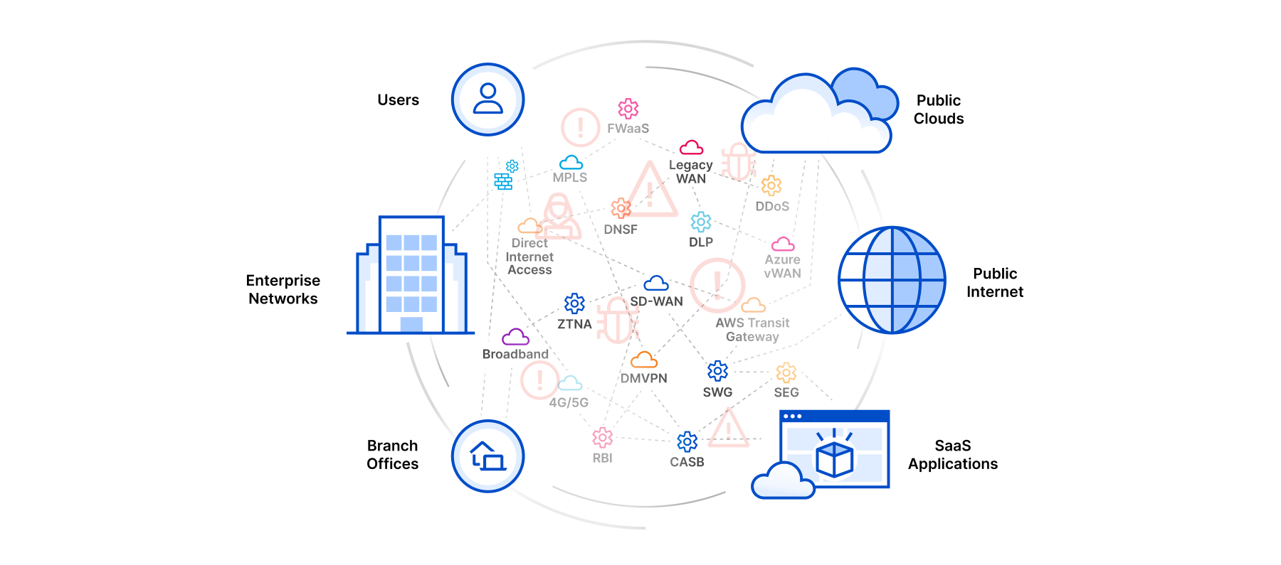
Frequently, an important part of customer conversations is being able to read between the lines. When customers speak about loss of control, they seem to be quietly wishing for something they think doesn’t exist. What they want is a connective tissue for everything IT and security are responsible for — something that reduces complexity by working with everything in the environment, being available everywhere, and performing whatever security, networking, and development functions are needed.
Further research confirmed our suspicions. Surveys of IT and security leaders indicate that 72% would highly value a secure “any-to-any” cloud platform. And they said they would invest an average of 16% of their entire IT and security budget in such a platform.
That got us to thinking — what exactly would that sort of cloud platform look like? How would it accomplish everything it had to?
We’ve got answers to share: a connectivity cloud.
A connectivity cloud is a new approach for delivering the many services companies need to secure and connect their digital environment. It’s a unified, intelligent, platform of programmable cloud-native services that enable any-to-any connectivity between all networks (enterprise and internet), cloud environments, applications and users. It includes a huge array of security, performance, and developer services — not with an eye to replace everything everywhere, but with the ability to fit in wherever needed and consolidate many critical services onto a single platform.
A connectivity cloud is built around four fundamental principles.
With these qualities, the connectivity cloud lets you add new services to your digital environment without losing even more control — and also helps restore control to what you’ve already got.
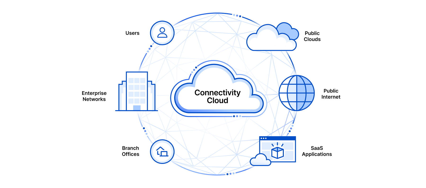
We’ll admit we’re predisposed to find those four qualities particularly important. From our earliest days, we’ve built our services based on the principles of integration, programmability, platform intelligence, and simplicity. And now, our overall portfolio is comprehensive enough to help customers achieve these benefits when tackling a huge array of security and IT needs.
Because of this approach, we’re proud to say that Cloudflare is the world’s first connectivity cloud.
But don’t take our word for it. Here are a few examples of customers that have used Cloudflare to help resolve their own crises of control:
A connectivity cloud’s programmability, deep network integration, and built-in intelligence make it ideal for delivering secure access to corporate resources.
The electronics retailer Conrad Electronic told us, “Just keeping people online created a series of administrative bottlenecks.” Nearly half of their 2,300 employees need to access corporate applications remotely. Enabling that access was burdensome: they had to deploy and configure VPN clients for each user.
Conrad Electronic now uses Cloudflare’s connectivity cloud to provide secure remote access to hundreds of corporate applications. Their management burden is significantly lower, with their team telling us they now have much more time per month to devote to improving their web operations. What’s more, their security posture is stronger: “We can restrict specific individuals or secure sensitive areas with a mouse click. Not having to maintain 1,000 VPN profiles improves our security and saves us time and money.”
A connectivity cloud’s threat intelligence, network integration, and unified interface also make it excellent at closing securing gaps and enabling secure application delivery on a global scale.
The multinational retail and wholesaling company Carrefour has a thriving and rapidly growing ecommerce presence. However, when cyber attacks ramped up, simply growing their security stack didn’t help. As their security team told us, “The interlacing of multiple tools complicated coordination and control of the architecture…additionally, the lack of integration across tools made investigating and resolving security and performance issues a complex and time-consuming effort.”
As part of their broader security transformation, they adopted Cloudflare’s connectivity cloud to prevent web exploits, zero-day threats, and malicious bot attacks. Doing so allowed them to replace five security tools from different vendors. And since then, they’ve reduced their incident resolution time by 75%.
Finally, a connectivity cloud’s programmability and network integration help it power innovative development in almost any context.
The global design juggernaut Canva is one example. Previously, they used a variety of developer platforms to run custom code at the network edge. But they found those services too time-consuming to use, and ran into limitations that held their innovation back.
Cloudflare’s connectivity cloud has become “a critical part of our software” They use the connectivity cloud’s developer services to build and run custom code, optimize page delivery for SEO, and time-limit content access. Recently, they told us “Thanks to Cloudflare, we can focus on growing our product and expanding into new markets with confidence, knowing that our platform is fast, reliable, and secure.”
What’s more, their experience has led to them also adopting Cloudflare’s for secure access and application delivery — a hugely gratifying example of a connectivity cloud operating at full power.
Customers are the inspiration for our innovation, and our connectivity cloud vision is no exception. We live to make things easier, faster, more secure and more connected – and it’s amazing to see how the connectivity cloud helps reduce complexity and increase security.
You can learn more about the connectivity cloud here — but we hope that’s just the beginning. Reach out to all of us at Cloudflare to ask questions and make suggestions — I look forward to continuing the conversation discovering ways we can continue to help customers on their secure, connected journey.

Post Syndicated from Phillip Jones original http://blog.cloudflare.com/sippy-incremental-migration-s3-r2/


Earlier in 2023, we announced Super Slurper, a data migration tool that makes it easy to copy large amounts of data to R2 from other cloud object storage providers. Since the announcement, developers have used Super Slurper to run thousands of successful migrations to R2!
While Super Slurper is perfect for cases where you want to move all of your data to R2 at once, there are scenarios where you may want to migrate your data incrementally over time. Maybe you want to avoid the one time upfront AWS data transfer bill? Or perhaps you have legacy data that may never be accessed, and you only want to migrate what’s required?
Today, we’re announcing the open beta of Sippy, an incremental migration service that copies data from S3 (other cloud providers coming soon!) to R2 as it’s requested, without paying unnecessary cloud egress fees typically associated with moving large amounts of data. On top of addressing vendor lock-in, Sippy makes stressful, time-consuming migrations a thing of the past. All you need to do is replace the S3 endpoint in your application or attach your domain to your new R2 bucket and data will start getting copied over.
Sippy is an incremental migration service built directly into your R2 bucket. Migration-specific egress fees are reduced by leveraging requests within the flow of your application where you’d already be paying egress fees to simultaneously copy objects to R2. Here is how it works:
When an object is requested from Workers, S3 API, or public bucket, it is served from your R2 bucket if it is found.
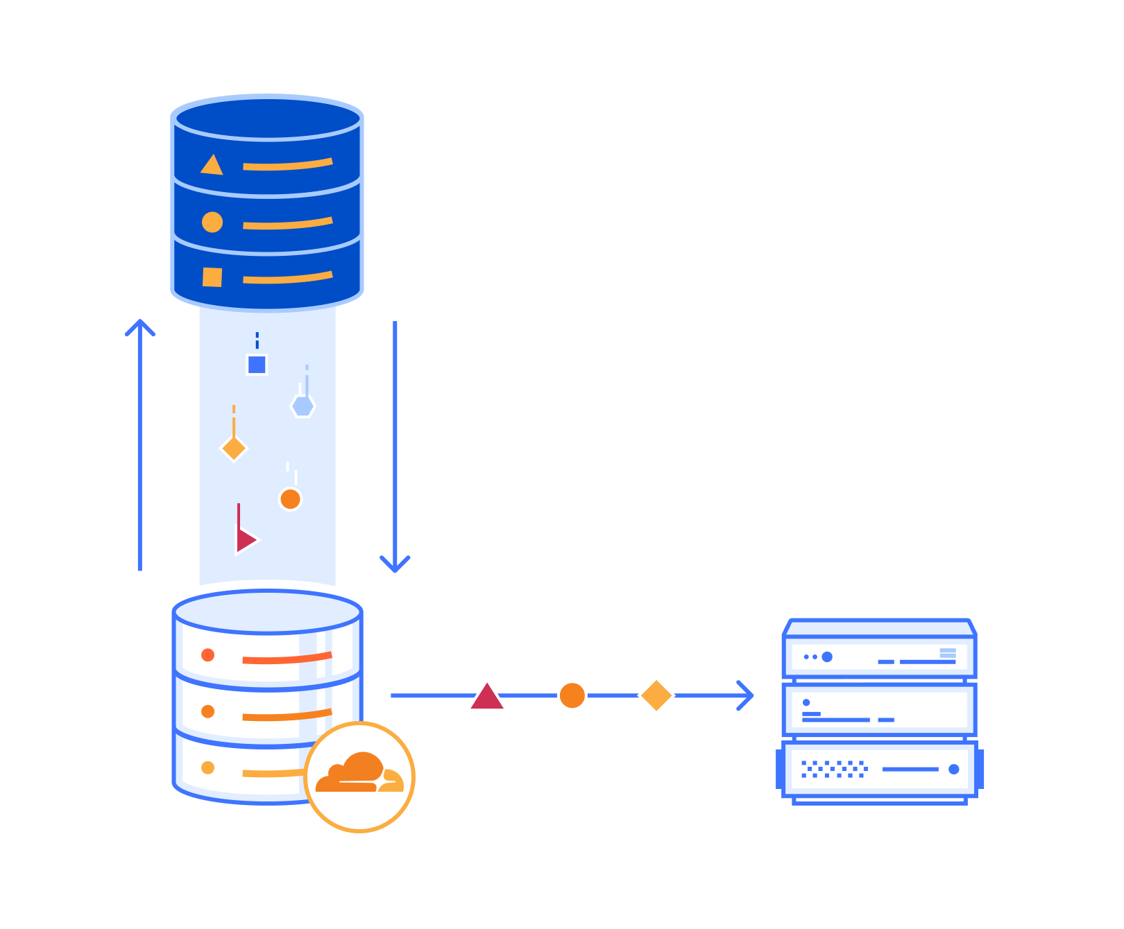
If the object is not found in R2, it will simultaneously be returned from your S3 bucket and copied to R2.
Note: Some large objects may take multiple requests to copy.
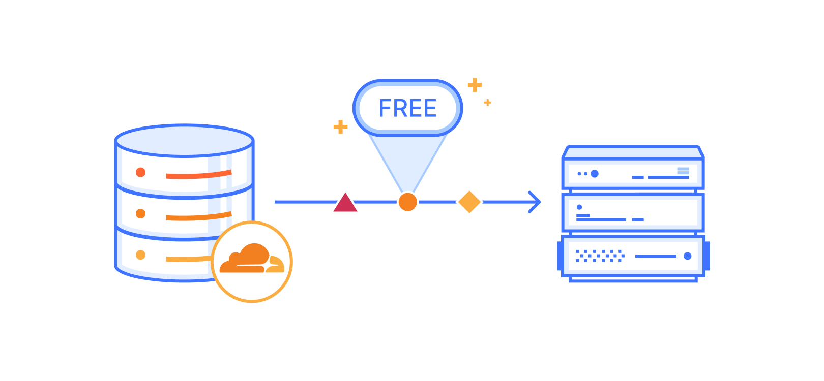
That means after objects are copied, subsequent requests will be served from R2, and you’ll begin saving on egress fees immediately.
To get started with incremental migration, you’ll first need to create an R2 bucket if you don’t already have one. To create a new R2 bucket from the Cloudflare dashboard:
To learn more about other ways to create R2 buckets refer to the documentation on creating buckets.
Next, you’ll enable Sippy for the R2 bucket you created. During the beta, you can do this by using the API. Here’s an example of how to enable Sippy for an R2 bucket with cURL:
curl -X PUT https://api.cloudflare.com/client/v4/accounts/{account_id}/r2/buckets/{bucket_name}/sippy \
--header "Authorization: Bearer <API_TOKEN>" \
--data '{"provider": "AWS", "bucket": "<AWS_BUCKET_NAME>", "zone": "<AWS_REGION>","key_id": "<AWS_ACCESS_KEY_ID>", "access_key":"<AWS_SECRET_ACCESS_KEY>", "r2_key_id": "<R2_ACCESS_KEY_ID>", "r2_access_key": "<R2_SECRET_ACCESS_KEY>"}'
For more information on getting started, please refer to the documentation. Once enabled, requests to your bucket will now start copying data over from S3 if it’s not already present in your R2 bucket.
You can run your incremental migration for as long as you want, but eventually you may want to complete the migration to R2. To do this, you can pair Sippy with Super Slurper to easily migrate your remaining data that hasn’t been accessed to R2.
We’re excited about open beta, but it’s only the starting point. Next, we plan on making incremental migration configurable from the Cloudflare dashboard, complete with analytics that show you the progress of your migration and how much you are saving by not paying egress fees for objects that have been copied over so far.
If you are looking to start incrementally migrating your data to R2 and have any questions or feedback on what we should build next, we encourage you to join our Discord community to share!