Tag Archives: Engineering

Using mobile sensor data to encourage safer driving

Post Syndicated from Grab Tech original https://engineering.grab.com/using-mobile-sensor-data-to-encourage-safer-driving

“Telematics”, a cross between the words telecommunications and informatics, was coined in the late 1970s to refer to the use of communication technologies in facilitating exchange of information. In the modern day, such technologies may include cloud platforms, mobile networks, and wireless transmissions (e.g., Bluetooth). Although the initial intention is for a more general scope, telematics is now specifically used to refer to vehicle telematics where details of vehicle movements are tracked for use cases such as driving safety, driver profiling, fleet optimisation, and productivity improvements.

We’ve previously published this article to share how Grab uses telematics to improve driver safety. In this blog post, we dive deeper into how telematics technology is used at Grab to encourage safer driving for our driver and delivery partners.

Background

At Grab, the safety of our users and their experience on our platform is our highest priority. By encouraging safer driving habits from our driver and delivery partners, road traffic accidents can be minimised, potentially reducing property damage, injuries, and even fatalities. Safe driving also helps ensure smoother rides and a more pleasant experience for consumers using our platform.

To encourage safer driving, we should:

  1. Have a data-driven approach to understand how our driver and delivery partners are driving.
  2. Help partners better understand how to improve their driving by summarising key driving history into a personalised Driving Safety Report.

Understanding driving behaviour

One of the most direct forms of driving assessment is consumer feedback or complaints. However, the frequency and coverage of this feedback is not very high as they are only applicable to transport verticals like JustGrab or GrabBike and not delivery verticals like GrabFood or GrabExpress. Plus, most driver partners tend not to receive any driving-related feedback (whether positive or negative), even for the transport verticals.

A more comprehensive method of assessing driving behaviour is to use the driving data collected during Grab bookings. To make sense of these data, we focus on selected driving manoeuvres (e.g., braking, acceleration, cornering, speeding) and detect the number of instances where our data shows unsafe driving in each of these areas.

We acknowledge that the detected instances may be subjected to errors and may not provide the complete picture of what’s happening on the ground (e.g., partners may be forced to do an emergency brake due to someone swerving into their lane).

To address this, we have incorporated several fail-safe checks into our detection logic to minimise erroneous detection. Also, any assessment of driving behaviour will be based on an aggregation of these unsafe driving instances over a large amount of driving data. For example, individual harsh braking instances may be inconclusive but if a driver partner displays multiple counts consistently across many bookings, it is likely that the partner may be used to unsafe driving practices like tailgating or is distracted while driving.

Telematics for detecting unsafe driving

For Grab to consistently ensure our consumers’ safety, we need to proactively detect unsafe driving behaviour before an accident occurs. However, it is not feasible for someone to be with our driver and delivery partners all the time to observe their driving behaviour. We should leverage sensor data to monitor these driving behaviour at scale.

Traditionally, a specialised “black box” inertial measurement unit (IMU) equipped with sensors such as accelerometers, gyroscopes, and GPS needs to be installed in alignment with the vehicle to directly measure vehicular acceleration and speed. In this manner, it would be straightforward to detect unsafe driving instances using this data. Unfortunately, the cost of purchasing and installing such devices for all our partners is prohibitively high and it would be hard to scale.

Instead, we can leverage a device that all partners already have: their mobile phone. Modern smartphones already contain similar sensors to those in IMUs and data can be collected through the telematics SDK. More details on telematics data collection can be found in a recently published Grab tech blog article1.

It’s important to note that telematics data are collected at a sufficiently high sampling frequency (much more than 1 Hz) to minimise inaccuracies in detecting unsafe driving instances characterised by sharp acceleration impulses.

Processing mobile sensor data to detect unsafe driving

Unlike specialised IMUs installed in vehicles, mobile sensor data have added challenges to detecting unsafe driving.

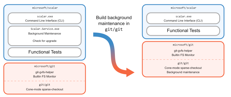
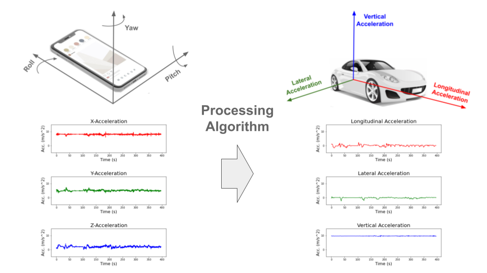
Accounting for orientation: Phone vs. vehicle

The phone is usually in a different orientation compared to the vehicle. Strictly speaking, the phone accelerometer sensor measures the accelerations of the phone and not the vehicle acceleration. To infer vehicle acceleration from phone sensor data, we developed a customised processing algorithm optimised specifically for Grab’s data.

First, the orientation offset of the phone with respect to the vehicle is defined using Euler angles: roll, pitch and yaw. In data windows with no net acceleration of the vehicle (e.g., no braking, turning motion), the only acceleration measured by the accelerometer is gravitational acceleration. Roll and pitch angles can then be determined through trigonometric manipulation. The complete triaxial accelerations of the phone are then rotated to the horizontal plane and the yaw angle is determined by principal component analysis (PCA).

An assumption here is that there will be sufficient braking and acceleration manoeuvring for PCA to determine the correct forward direction. This Euler angles determination is done periodically to account for any movement of phones during the trip. Finally, the raw phone accelerations are rotated to the vehicle orientation through a matrix multiplication with the rotation matrix derived from the Euler angles (see Figure 1).

Figure 1: Inference of vehicle acceleration from the phone sensor data. Smartphone and car images modified from designs found in Freepik.com.

Handling variations in data quality

Our processing algorithm is optimised to be highly robust and handle large variations in data quality that is expected from bookings on the Grab platform. There are many reported methods for processing mobile data to reorientate telematics data for four wheel vehicles23.

However, with the prevalent use of motorcycles on our platform, especially for delivery verticals, we observed that data collected from two wheel vehicles tend to be noisier due to differences in phone stability and vehicular vibrations. Data noise can be exacerbated if partners hold the phone in their hand or place it in their pockets while driving.

In addition, we also expect a wide variation in data quality and sensor availability from different phone models, such as older, low-end models to the newest, flagship models. A good example to illustrate the robustness of our algorithm is having different strategies to handle different degrees of data noise. For example, a simple low-pass filter is used for low noise data, while more complex variational decomposition and Kalman filter approaches are used for high noise data.

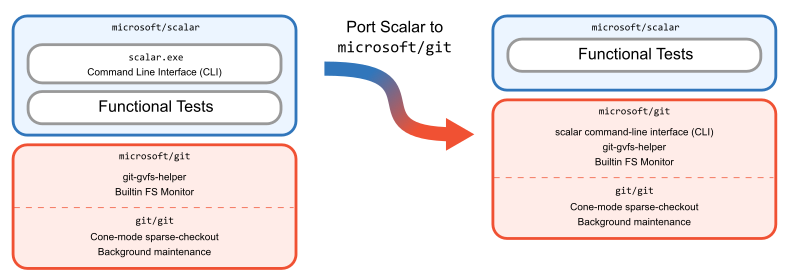
Detecting behaviour anomalies with thresholds

Once the vehicular accelerations are inferred, we can use a thresholding approach (see Figure 2) to detect unsafe driving instances.

For unsafe acceleration and braking, a peak finding algorithm is used to detect acceleration peaks beyond a threshold in the longitudinal (forward/backward) direction. For unsafe cornering, older and lower end phones are usually not equipped with gyroscope sensors, so we should look for peaks of lateral (sidewards) acceleration (which constitutes the centripetal acceleration during the turn) beyond a threshold. GPS bearing data that coarsely measures the orientation of the vehicle is then used to confirm that a cornering and not lane change instance is being detected. The thresholds selected are fine-tuned on Grab’s data using initial values based on published literature4 and other sources.

To reduce false positive detection, no unsafe driving instances will be flagged when:

  1. Large discrepancies are observed between speeds derived from integrating the longitudinal (forward/backward) acceleration and speeds directly measured by the GPS sensor.
  2. Large phone motions are detected. For example, when the phone falls to the seat from the dashboard, accelerations recorded on the phone sensor will deviate significantly from the vehicle accelerations.
  3. GPS speed is very low before and after the unsafe driving instance is detected. This is limited to data collected from motorcycles which is usually used by delivery partners. It implies that the partner is walking and not in a vehicle. For example, a GrabFood delivery partner may be collecting the food from the merchant partner on foot, so no unsafe driving instances should be detected.
Figure 2: Animation showing unsafe driving detection by thresholding. Dotted lines in acceleration charts indicate selected thresholds. Map tiles by stamen design.

Detecting speeding instances from GPS speeds and map data

To define speeding along a stretch of road, we used a rule-based method by comparing raw speeds from GPS pings with speeding thresholds for that road. Although GPS speeds are generally accurate (subjected to minimal GPS errors), we need to take more precautions to ensure the right speeding thresholds are determined.

These thresholds are set using known speed limits from available map data or hourly aggregated speed statistics where speed limits are not available. The coverage and accuracy of known speed limits is continuously being improved by our in-house mapping initiatives and validated comprehensively by the respective local ground teams in selected cities.

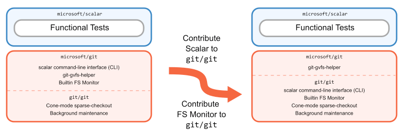
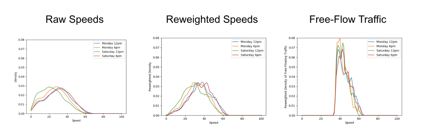
Aggregating GPS pings from Grab driver and delivery partners can be a helpful proxy to actual speed limits by defining speeding violations as outliers from socially acceptable speeds derived from partners collectively. To reliably compute aggregated speed statistics, a representative speed profile for each stretch of road must first be inferred from raw GPS pings (see Figure 3).

As ping sampling intervals are fixed, more pings tend to be recorded for slower speeds. To correct the bias in the speed profile, we reweigh ping counts by using speed values as weights. Furthermore, to minimise distortions in the speed profile from vehicles driving at lower-than-expected speeds due to high traffic volumes, only pings from free-flowing traffic are used when inferring the speed profile.

Free-flowing traffic is defined by speeds higher than the median speed on each defined road category (e.g., small residential roads, normal primary roads, large expressways). To ensure extremely high speeds are flagged regardless of the speed of other drivers, maximum threshold values for aggregated speeds are set for each road category using heuristics based on the maximum known speed limit of that road category.

Figure 3: Steps to infer a representative speed profile for computing aggregated speed statistics.

Besides a representative speed profile, hourly aggregation should also include data from a sufficient number of unique drivers depending on speed variability. To obtain enough data, hourly aggregations are performed on the same day of the week over multiple weeks. This way, we have a comprehensive time-specific speed profile that accounts for traffic quality (e.g., peak hour traffic, traffic differences between weekdays/weekends) and driving conditions (e.g., visibility difference between day/night).

When detecting speeding violations, the GPS pings used are snapped-to-road and stationary pings, pings with unrealistic speeds, while pings with low GPS accuracy (e.g., when the vehicle is in a tunnel) are excluded. A speeding violation is defined as a sequence of consecutive GPS pings that exceed the speeding threshold. The following checks were put in place to minimise erroneous flagging of speeding violations:

  1. Removal of duplicated (or stale) GPS pings.
  2. Sufficient speed buffer given to take into account GPS errors.
  3. Sustained speeding for a prolonged period of time is required to exclude transient speeding events (e.g., during lane change).

Driving safety report

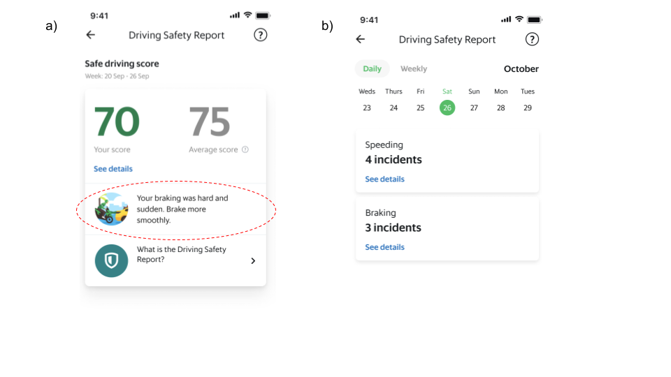
The driving safety report is a platform safety product that driver and delivery partners can access via their driver profile page on the Grab Driver Application (see Figure 4). It is updated daily and aims to create awareness regarding driving habits by summarising key information from the processed data into a personalised report that can be easily consumed.

Individual reports of each driving manoeuvre (e.g., braking, acceleration, cornering and speeding) are available for daily and weekly views. Partners can also get more detailed information of each individual instance such as when these unsafe driving instances were detected.

Figure 4: Driving safety report for driver and delivery partners using four wheel vehicles. a) Actionable insights feature circled by red dotted lines. b) Daily view of various unsafe driving instances where more details of each instance can be viewed by tapping on “See details”.

Actionable insights

Besides compiling the instances of unsafe driving in a report to create awareness, we are also using these data to provide some actionable recommendations for our partners to improve their driving.

With unsafe driving feedback from consumers and reported road traffic accident data from our platform, we also train machine learning models to identify patterns in the detected unsafe driving instances and estimate the likelihood of partners receiving unsafe driving feedback or getting into accidents. One use case is to compute a safe driving score that equates a four-wheel partner’s driving behaviour to a numerical value where a higher score indicates a safer driver.

Additionally, we use Shapley additive explanation (SHAP) approaches to determine which driving manoeuvre contributes the most to increasing the likelihood of partners receiving unsafe driving feedback or getting into accidents. This information is included as an actionable insight in the driving safety report and helps partners to identify the key area to improve their driving.

What’s next?

At the moment, Grab performs telematics processing and unsafe driving detections after the trip and updates the report the next day. One of the biggest improvements would be to share this information with partners faster. We are actively working on developing a real-time processing algorithm that addresses this and also, satisfies the robustness requirements such that partners are immediately aware after an unsafe driving instance is detected.

Besides detecting typical unsafe driving manoeuvres, we are also exploring other use cases for mobile sensor data in road safety such as detection of poor road conditions, counterflow driving against traffic, and phone usage leading to distracted driving.

Join us

Grab is the leading superapp platform in Southeast Asia, providing everyday services that matter to consumers. More than just a ride-hailing and food delivery app, Grab offers a wide range of on-demand services in the region, including mobility, food, package and grocery delivery services, mobile payments, and financial services across 428 cities in eight countries.

Powered by technology and driven by heart, our mission is to drive Southeast Asia forward by creating economic empowerment for everyone. If this mission speaks to you, join our team today!

References

  1. Burhan, W. (2022). How telematics helps Grab to improve safety. Grab Tech Blog. https://engineering.grab.com/telematics-at-grab 

  2. Mohan, P., Padmanabhan, V.N. and Ramjee, R. (2008).Nericell: rich monitoring of road and traffic conditions using mobile smartphones. SenSys ‘08: Proceedings of the 6th ACM conference on Embedded network sensor systems, 312-336. https://doi.org/10.1145/1460412.1460444 

  3. Sentiance (2016). Driving behavior modeling using smart phone sensor data. Sentiance Blog. https://sentiance.com/2016/02/11/driving-behavior-modeling-using-smart-phone-sensor-data/ 

  4. Yarlagadda, J. and Pawar, D.S. (2022). Heterogeneity in the Driver Behavior: An Exploratory Study Using Real-Time Driving Data. Journal of Advanced Transportation. vol. 2022, Article ID 4509071. https://doi.org/10.1155/2022/4509071 

The Story of Scalar

Post Syndicated from Derrick Stolee original https://github.blog/2022-10-13-the-story-of-scalar/

When you install Git v2.38, you’ll find a new executable tool available called scalar. At its core, Scalar enables the latest and greatest Git features for working with large repositories. By simply switching from git clone to scalar clone, you will have all of Git’s most impactful performance features, such as partial clone, sparse-checkout, background maintenance, and advanced config options neatly configured for your repository. Have you already cloned your repository? Run scalar register in it to get the same features.

Scalar and Git, together at last

Although Scalar is only now making its formal Git debut, this release represents the culmination of a multi-year journey. Today, we will share the story of how Scalar got to this point. We’ll start from what inspired its creation, how it evolved from a prototype carved out of the VFS for Git codebase, and finally how it landed in upstream Git. Each step of the way was guided by a set of development principles that helped us with each challenge and opportunity.

Special thanks to @chrisd8088, @dscho, @jeffhostetler, @jrbriggs, @kyle-rader, @mjcheetham, @ldennington, @prplr, @wilbaker, and all of the other contributors who helped make this happen!

Our development principles

Before we get into specifics about how Scalar was built and eventually rewritten and contributed upstream, we need to first establish some context. We entered the project with certain values that we used to guide our decisions. Here are a few that are particularly important to this story.

Rapid prototyping

Code speaks volumes. We could design an architecture all we want on paper, but when solving problems at scale, we need to have actual code running before we can make a final decision.

Before committing to a decision, we would quickly build a prototype and measure its performance. During this prototyping phase, we would take shortcuts to get to that point of measurement. Then, we’d throw everything we could at the prototype to make sure it was correct and fast.

Based on the prototype, we would commit to doing the careful engineering of building the feature again but with a test strategy, thoughtful architecture, and a plan for delivering it to users.

Incremental changes over complete rewrites

Looking at where we started to where we ended, it might seem like we are proponents of rewriting things from scratch. We intend to demonstrate exactly the opposite: Scalar moved with small incremental changes that solved an immediate need. While making those changes, we also optimized for reducing our technical debt and creating a better architecture, and that resulted in code moving from .NET to C and then from our fork to upstream Git, but each individual movement was relatively small compared to the entire system.

The biggest reason we focused on incremental changes was because of our next value.

Tests are an asset

Making any kind of software change adds risk to a project. That risk is mitigated when we have a large set of battle-hardened tests. With a robust test suite available, we were able to make significant changes to our architecture with confidence.

Work in the open

Other than the earliest prototypes, all changes were reviewed and merged completely in public, either in the microsoft/scalar repository or the microsoft/git repository. Scalar was an open source project from day one, and was never intended to be a project only for internal use. By contrast, VFS for Git was built as a tool for Microsoft’s internal use first, and open sourcing it was a bonus after it reached enough adoption. Not only did we value that transparency during Scalar’s development, but now we have a history of public code changes to talk about here.

Now that we’ve established these values, let’s begin the story of Scalar.

A catalyst forces a pivot

The Virtual FileSystem for Git project (VFS for Git for short—previously “GVFS”) was built specifically to transition the Microsoft Windows OS monorepo to Git. VFS for Git utilizes a virtual filesystem to lazily load files only when a filesystem read occurs. This greatly reduced the amount of work Git needed to do, but required installing the microsoft/git fork as well as the .NET VFS for Git software and use Azure Repos to host the repository.

Initially, the Microsoft Office monorepo was going to onboard to Git using VFS for Git, but they needed cross-platform support, specifically for macOS development. After getting pretty far in a macOS port, Apple deprecated the kernel features that provided the filesystem virtualization that was required for that flow.

We were in luck, however, because we had come to understand something a key quality of the Office monorepo: Office has a rigorous dependency system that clearly identifies which files are necessary for a local build. This means that a developer could specify the files they need to Git’s sparse-checkout feature instead of dynamically populating the worktree using a virtual filesystem. This also significantly simplifies the software needed to manage their monorepo!

However, there was a problem. The sparse-checkout feature had previously been abandoned as a direction for VFS for Git due to its performance. Git would use a list of patterns to match which paths should be in the worktree and which should be ignored. This pattern matching had an ordering strategy that required iterating through the entire pattern list for every possible path, requiring quadratic time! For one of the larger sparse-checkout definition examples we had, Git would take 40 minutes to evaluate the sparse-checkout patterns.

Sparse-checkout definitions are extremely generic. They include matching on file prefix, but also file suffix, or path substring, and any combination. For our target monorepo, we only needed directory matches. With that limited type of pattern in mind, we added a new mode to Git’s sparse-checkout feature: “cone mode” sparse-checkout. A quick prototype of cone mode sparse-checkout demonstrated that Git could reach similar performance as VFS for Git, especially when paired with the filesystem monitor hook. Our critical performance measurement was the git status command, and we were seeing performance within three or four seconds, which was close to the typical case in VFS for Git.

This was promising enough to move forward with a full prototype. We decided to make this a separate project from VFS for Git, so it needed its own name: Scalar.

Throw the first one away

Once we had a handle on Git command performance using Git’s sparse-checkout feature, we needed to adapt all of the code that allowed fast clones and fetches to work within that environment. For most Git hosting services, Git’s partial clone feature is the best way to solve for fast clones and fetches. However, Azure Repos has an earlier version that was built for VFS for Git called the GVFS protocol. We needed a way to speak the GVFS protocol to bootstrap clones and to dynamically fetch missing objects during Git commands.

This was our first point of asking, “Should we rewrite, or refactor?” The VFS for Git codebase already had all of the client-side code for speaking the GVFS protocol. Not only that, it also had a large set of end-to-end tests that constructed a complete clone from Azure Repos and then ran thousands of Git commands in that environment to make sure they operated exactly the same as a normal Git clone. Since those tests were a significant asset, we set out to construct the first version of this new project starting with the VFS for Git code.

In this initial prototype, we just wanted to get things working for the end-to-end tests to pass. This process included disabling the virtual filesystem code, but leaving all of the hooks that enabled the GVFS Protocol. We also needed to set up sparse-checkout at clone time before initializing the HEAD reference. This prototype was so rough it still didn’t have the Scalar name: it still operated as if it was the gvfs command-line interface.

Diagram showing that the pre-Scalar prototype mostly deleted code from the GVFS protocol.
The rapid prototyping phase mostly deleted code

The end result wasn’t pretty. We couldn’t hope to ship it since it would break compatibility with previous VFS for Git versions. The tests were cobbled together to make things work, but we had disabled sparse-checkout in the tests since the previous tests assumed that every path could be populated dynamically with the virtual filesystem. However, we got to a point where we could reliably create this new repository setup and measure its success. Since the clones were doing the exact same thing as in VFS for Git, the performance matched exactly. Now, we needed to rebuild it, and do it the right way.

Get to Minimum Viable Product (MVP)

From the success of our initial prototype, we moved on to creating an MVP that we could demo to internal users. Here is where we created the Scalar name, the microsoft/scalar repository, and started doing thorough reviews of all changes.

As a team, we decided it would be best to create a new repository rather than to build the project within the VFS for Git codebase. We did not want to be locked into the architecture of VFS for Git as we moved forward, and we also wanted to take advantage of the commit history for the code in the repository. The first task in creating the new project was renaming all references to the old project.

Diagram detailing that, between the pre-Scalar prototype and the version pushed to microsoft/git, many pieces were renamed.
Cleaning up the prototype and renaming things

Updating tests

The next step we had to do was to make sure that we were sufficiently testing the sparse-checkout environment. Recall that we used the full worktree to get tests passing in the prototype, but now we needed to actually be sure that our sparse-checkout environment would work properly.

For this, we found a minimal set of patterns that would include all of the concrete paths used by the test suite.

Then, we made sure that there were interesting changes happening outside of those patterns that would exercise Git features like git merge or git cherry-pick in interesting ways outside of the sparse-checkout definition.

Finally, we added specific tests that involved changing the sparse-checkout definition to make sure that Git would properly fill in the missing files. In this way, we were able to keep all of the existing tests while also adding new tests that were specific to our environment.

Evaluating the MVP

After completing the product changes and test updates, it was time to evaluate the solution. We ran performance numbers to ensure they matched what we saw in our prototype phase. We created local clones to use in daily work to try and catch any lingering bugs.

But it all came down to evaluating the solution with internal users. We demoed Scalar directly with the Office engineering system team and asked pointed questions about whether this would work for them.

In particular, we were worried about the performance of git checkout. In VFS for Git, git checkout is extremely fast because it doesn’t actually do much work. It clears the filesystem of concrete files and replaces them with virtualized files. The cost of populating the filesystem comes later when those files are read by an IDE or a build process. With Scalar, the filesystem is populated within the git checkout process, so that work is now upfront and clear to the user.

By working directly with the engineering system team, we learned that this git checkout performance was not an issue. Since git checkout changes source files, it invalidates the local build. Build times can take hours in this monorepo after taking new changes, so users typically do not use git checkout until the end of the day when they are ready to trigger a long build overnight. For this reason, git checkout was not a critical path for their developers. In fact, there was great interest in being able to know that they could disconnect from the network and still poke around the code without risk of finding a virtual file.

We were good to go with our plan for Scalar. However, the monorepo team needed to build something of their own. They needed a connection between their build system and sparse-checkout. While they built that, we had time to polish Scalar and make it easier to install and use.

Update architecture under stable conditions

With the benefit of a stable test suite and a few months of runway, we were able to take our MVP and rethink the architecture. In particular, we shed some architectural decisions that were critical to how VFS for Git works, but were no longer needed in Scalar.

VFS for Git requires a process running that can handle requests from the filesystem to populate virtualized content on-demand. The existence of this process creates the concept of a “mounted” repository, and even included the commands gvfs mount and gvfs unmount to toggle this state.

Because this process needed to exist, a lot of other things were placed in that process that could be relocated elsewhere in Scalar. We set out to remove the need for this process.

Since we had already removed the virtual filesystem code, there were two remaining pieces that were in the mount process: performing background maintenance and downloading objects via the GVFS protocol.

For background maintenance, we took the fastest approach and moved the scheduled tasks out of the mount process and into the Scalar.Service global singleton process. We had versions of this service for Windows and macOS to handle things like startup operations. Moving the maintenance tasks to this service was quick and easy.

For the object downloads, it was a bigger job. The existing architecture included a read-object hook custom to microsoft/git that was installed by the scalar clone command, and that hook communicated to the mount process which actually communicated with the server and placed the objects in the repository.

For this, we created a tool within microsoft/git to do these missing object queries via the GVFS protocol directly within the Git codebase. This tool lives underneath the code that fills in objects for Git’s partial clone feature. By connecting this tool to partial clone, we could work to improve partial clone while also helping Scalar users at the same time. One major benefit to working within the partial clone framework is that some missing object requests can be batched together into a single request, while the old read-object hook could only ask for one missing object at a time.

Finally, there was nothing important remaining in the mount process, so we deleted it. In addition, we were able to delete the old Git hook.

At this point, we had simplified the architecture to have fewer moving parts and were ready to ship internally.

Diagram showing that removing the mount process simplified Scalar's architecture.
Removing the mount process with the git-gvfs-helper

Upon success, look for low-hanging fruit

Shortly after announcing Scalar to the world, we realized that Scalar could have a larger benefit to the Git ecosystem than just very large monorepos using Azure Repos.

We extended scalar clone to use Git’s partial clone if the remote did not speak the GVFS protocol. In this way, scalar clone became something a user could run against any Git remote.

This was an inflection point in our lifecycle: we had accomplished what we set out to do, but wanted to put these tools in front of more people and find a wider audience. We started to shift our focus from making updates in the .NET project and instead contributing features to the upstream Git project.

Rethink architecture as conditions change

Up until this point, we were using the existing hook approach that speaks to a third-party filesystem monitor. This meant that we needed to install that third-party tool next to Scalar, but also scalar clone would install the hook in addition to all of its other operations. We realized that we could solve our installation complexities, reduce the complexity of scalar clone, and get faster performance if the filesystem monitor was built into Git. With that context, we began building Git’s builtin filesystem monitor. We took early versions into microsoft/git while it was reviewed carefully by the Git community.

Diagram showing early adoption of the builtinFS Monitor.
Early adoption of builtin FS Monitor

An important Scalar feature was background maintenance, which was accomplished by a service running in the background and launching Git commands at certain intervals to keep data fresh and well-organized. This service existed from the VFS for Git days, so it was easy to keep using it on Windows and macOS. However, when the Office team told us that they needed Linux clients to support some of their web developers, we focused on porting Scalar to Linux. This service was one platform-specific part that would be difficult to implement in .NET.

We decided that instead of creating a new service in Scalar, it would be better to implement background maintenance in Git. Once Git had its own cross-platform way of doing maintenance, Scalar could stop using its custom logic and instead rely on git maintenance run.

We then removed the service from Scalar.

Diagram showing that removing background maintenance from Scalar left only the CLI and tests.
Background maintenance leaves us with only the CLI and tests

After making this change, we took another look at our architecture and realized something. Suddenly, Scalar was only a command-line interface on top of Git. Why have it be in C#, separate from the Git source code?

The overhead of dealing with Scalar as a .NET tool was colliding with our maintenance costs of creating releases and shipping it to users. If Office developers require the microsoft/git fork of Git and another tool then things get tricky when we want to release a new version.

We had replaced so many features in the Scalar codebase with Git functionality that starting from a clean slate could allow us to build a more manageable architecture than that of the existing code. Also, by inserting the Scalar CLI into the Git codebase, we could take advantage of internal functions such as using Git config APIs instead of running git config processes to set recommended config values.

With these goals in mind, we ported the Scalar CLI to C in microsoft/git using less than 3,000 lines of code!

This endeavor to recreate the Scalar CLI in the microsoft/git codebase can best be appreciated by seeing that we deleted over 10 times the amount of code from microsoft/scalar than we added to microsoft/git when we removed all product code. We kept the microsoft/scalar repository around as a collection of tests, allowing us to be confident in the new code.

Diagram showing that once the CLI was ported to microsoft/git, only the tests were left behind.
Porting the CLI to microsoft/git leaves only the tests

This was our biggest step in the journey because it involved the largest rewrite of Scalar code. However, the requirements of the Scalar CLI at this point were well-defined and greatly simplified from earlier. We were able to immediately celebrate by no longer shipping the .NET Scalar application to our internal customers and instead rely on just shipping the microsoft/git fork.

There was one downside to this change, though. Before, you could install the .NET Scalar solution on top of any Git version and still get all the benefits of scalar clone. Now, users needed to replace their Git client with microsoft/git in order to get the latest Scalar version. We wanted to make Scalar useful to everyone, not just those that were willing to install our fork.

The journey into core Git

Porting Scalar to C not only enabled hosting the tool in microsoft/git, it opened up the possibility of making Scalar part of the upstream Git project. Although it wouldn’t be the first feature originating in microsoft/git that was contributed upstream, there was no clear precedent for something like Scalar: a standalone executable whose name didn’t start with git in the Git project. That might sound like nothing more than an implementation detail, but it represented a philosophical departure from the existing tools in Git. This divergence would drive us to define what Scalar meant for Git.

contrib/-uting to Git

From the outset, we knew there was a contingent of Git users that would benefit from Scalar beyond microsoft/git‘s typical user base. Features like the filesystem monitor, background maintenance, cone mode sparse-checkout, etc. had all become popular among developers in large repositories. Scalar exposed those and a multitude of other features more readily to users. Still, it wasn’t clear that Scalar as a standalone executable was the best—or Git-friendliest—way to present those features.

To gradually introduce the tool to the Git community, Scalar’s journey upstream began in Git’s contrib/ directory. From the contrib/ README:

Although these pieces are available as part of the official git
source tree, they are in somewhat different status.  The
intention is to keep interesting tools around git here, maybe
even experimental ones, to give users an easier access to them,
and to give tools wider exposure, so that they can be improved
faster.

Despite the loose requirements of contrib/, the submitted version of Scalar still required some changes from what was in microsoft/git. First was removing the GVFS protocol-supported clones. As we mentioned earlier, blobless clones were introduced into Scalar as a fallback for clones using the GVFS protocol, so the upstream version defaulted to using blobless partial clones instead. Additionally, to preserve the separation between contrib/ and the main Git repository, the GitHub Actions workflow was also stripped of references to Scalar, including execution of the microsoft/scalar test suite.

However, being in contrib/ did have some drawbacks. In order to build and install Scalar, a user needed to not only build Git from source, but know to navigate into contrib/scalar/ and build that as well. The separate build and test process also left it prone to changes in the rest of Git unintentionally breaking it. Even with these challenges, this arrangement was exactly what Scalar needed while its features were built out and long-term plan was developed. As we drew closer to finishing those features, we needed to finally answer the question: what should we do with Scalar?

Home sweet home

As soon as the possibility of upstreaming Scalar materialized, there were lots of ideas about what its final form would look like. One popular idea—which can be found in the original RFC—was to dissolve Scalar into a collection of new git commands and options to existing commands. Another was to have scalar reside in the Git tree in a dedicated subdirectory, like gitk. Another was to reimagine it as a Git built-in command: something like git scalar. Along with these implementation decisions came overarching questions of maintenance and relevance to Git.

As the tool was nearing feature completion upstream and the downsides of contrib/ isolation were weighing on the project, we took a step back and revisited the questions of Scalar’s identity. The result was a proposal to update Scalar’s documentation and outline a three-part approach to making the tool generally available in Git:

  1. Add any remaining large repo performance features to Scalar.
  2. Extract the parts of Scalar that are generally applicable to all Git users into built-in commands and/or options.
  3. Move Scalar into the root tree of Git, built and installed as a standalone executable alongside git.

The crux of this approach was a new framing of Scalar within the Git project. Scalar began, like VFS for Git before it, as a tool with its own features and opinions: how to configure a repository, what workflows to use, etc. As it evolved, those features and opinions were folded into Git or adjusted to align better with the upstream project, leaving Scalar with only the parts that fit the very specific role of configuring large repositories. In essence, Git had a user experience niche left by its myriad of large repo-focused performance features. Scalar filled that niche.

The roadmap to Scalar’s completion emerged from this philosophy. First, a few more particularly impactful features would be added to it (namely, the built-in FSMonitor). Then, because Scalar’s purpose is to configure features for large repositories that aren’t set up by default in Git, the parts that serve all Git users (such as repository diagnostics in scalar diagnose) would be extracted into new or existing Git commands. Finally, Scalar would be moved out of contrib/ and into the main build of the repository, intended to continue existing as a dedicated tool for managing large Git repositories.

The best laid plans often go awry but, fortunately, this one didn’t. Over the course of three upstream patch series, Scalar was streamlined inside of contrib/, then moved into its new home as part of core Git. And just in time for the v2.38.0 release!

Diagram showing that the Scalar project was contributed to git/git.
Scalar now lives in the core git/git project

The past, present, and future of Scalar

We’ve shared the story of Scalar not only to publicize a new and exciting feature in Git (seriously, go try it!), but also to illustrate one of the many paths an open source project can take to reach its users. Planning and re-planning, designing and redesigning, and no shortage of engineering lessons were all necessary steps to make Scalar the powerful tool it is today.

It is now a fully-integrated part of Git, but Scalar’s journey is far from over. Scalability and performance in Git is a hot topic—our own engineering blog is a testament to that—and consistent improvement in that area will undoubtedly be part of Scalar’s future. Today, though, Scalar’s eventful history is what has shaped it into the best way to unlock Git’s full potential on your largest repositories.

GitHub Availability Report: September 2022

Post Syndicated from Jakub Oleksy original https://github.blog/2022-10-05-github-availability-report-september-2022/

In September, we experienced one incident that resulted in significant impact and degraded state of availability to multiple GitHub services. We also experienced one incident resulting in significant impact to Codespaces. We are still investigating that incident and will include it in next month’s report. This report also sheds light into an incident that impacted Codespaces in August and an incident that impacted GitHub Actions in August.

September 8 19:44 UTC (lasting 5 hours and 11 minutes)

On September 8, 2022 at 19:44 UTC, our monitoring detected an increase in the number of pull request merge failures. The impact was concentrated on Enterprise Managed Users (EMUs) with a small number of bot accounts also affected.

Within 45 minutes, we traced the cause to a data transition that removed inconsistent data from profile records. Unfortunately, the transition incorrectly operated on EMU accounts, removing some data that is required to successfully merge pull requests via the UI and our API. CLI merges were unaffected.

We restored the data from backup, but this took longer than we had anticipated. We simultaneously pursued a workaround in code, but opted not to proceed with it as it could introduce data inconsistencies. Our restore operation resolved the issue with our pull request monitors having recovered by September 9, 2022 at 00:55 UTC.

Following this incident, we have made changes to our data transition procedures to allow for faster restores and transitions that can be automatically rolled back without relying on backups. We are also working on multiple improvements to our testing processes as they relate to EMUs.

September 28 03:53 UTC (lasting 1 hour and 16 minutes)

Our alerting systems detected an incident that impacted most Codespaces customers. Due to the recency of this incident, we are still investigating the contributing factors and will provide a more detailed update on cause and remediation in the October Availability Report, which we will publish the first Wednesday of November.

Follow up to August 29 12:51 UTC (lasting 5 hours and 40 minutes)

On August 29, 2022 at 12:51 UTC, our monitoring detected an increase in Codespaces create and start errors. We also started seeing DNS-related networking errors in some running Codespaces where outbound DNS resolutions were failing. At 14:19 UTC, we updated the status for Codespaces from yellow to red due to broad user impact.

This incident was caused by an Ubuntu security patch in systemd that broke DNS resolution. In recent versions of Ubuntu, unattended upgrades for security fixes are enabled by default. Codespaces host VMs were using the default recommended settings to apply security patches automatically on running VMs. When this patch was published, Codespaces host VMs started installing and applying the patch after the VM was created. Once the patch was installed on a VM, DNS resolution was broken. Depending on the timing of when the patch was installed on the host VM, this led to a few different failure modes, including failure creating/starting Codespaces or failure, making outbound network calls inside of a codespace that was already running.

Once we identified systemd’s DNS resolver configuration as the source of these errors, we were able to mitigate the issue by disabling systemd’s DNS resolver and manually configuring an upstream DNS resolver IP address. We deployed a change to the DNS configuration on the host VMs at 18:13 UTC. By 18:21 UTC, we started seeing positive signs of recovery in our metrics and changed the status to yellow. Ten minutes later, at 18:31 UTC, all metrics were fully healthy and the incident was resolved.

Following this incident, we are updating our DNS configuration to reduce dependencies on systemd’s DNS resolver. We are also investigating whether we should continue to use unattended upgrades for security patches. Disabling unattended upgrades will give us more deterministic behavior at runtime, preventing external changes from breaking Codespaces. We will remain fully capable of quickly patching VMs across our fleet even with unattended upgrades disabled.

Follow up to August 18 14:33 UTC (lasting 3 hours and 23 minutes)

This incident occurred in August but was left out of the August report because it did not result in a widespread outage. Several GitHub Actions customers experienced issues because of the degradation so we decided to include it retroactively.

At 14:13 UTC, there was a sudden spike in traffic to GitHub Actions which resulted in a higher than usual write load on our services. A majority of our services handled this graciously, but one of our internal services that is used for generating security tokens started returning 503 Service Unavailable errors to requests, triggering an alert to the engineering team. Further investigation revealed that the token database was experiencing a performance degradation which, compounded by the increased load, caused us to hit the database’s max concurrent connections limit. This was made worse due to a mismatch between our client-side throttling limits and database capacity, which resulted in our throttling thresholds allowing more traffic than this database had capacity to handle.

We mitigated the issue by scaling up the impacted database while also allowing a higher number of concurrent connections to it. The impacted service went back to a healthy state and the incident was considered resolved at 17:36 UTC. In addition to the immediate actions, we have improved our monitoring and alerting to allow faster remediation. We are also evaluating changes to our throttling mechanisms to better account for this traffic pattern.

In summary

Please follow our status page for real-time updates on status changes. To learn more about what we’re working on, check out the GitHub Engineering Blog.

Highlights from Git 2.38

Post Syndicated from Taylor Blau original https://github.blog/2022-10-03-highlights-from-git-2-38/

The open source Git project just released Git 2.38, with features and bug fixes from over 92 contributors, 24 of them new. We last caught up with you on the latest in Git back when 2.37 was released.

To celebrate this most recent release, here’s GitHub’s look at some of the most interesting features and changes introduced since last time.

A repository management tool for large repositories

We talk a lot about performance in Git, especially in the context of large repositories. Returning readers of these blog posts will no doubt be familiar with the dozens of performance optimizations that have landed in Git over the years.

But with so many features to keep track of, it can be easy to miss out some every now and then (along with their corresponding performance gains).

Git’s new built-in repository management tool, Scalar, attempts to solve that problem by curating and configuring a uniform set of features with the biggest impact on large repositories. To start using it, you can either clone a new repository with scalar clone:

$ scalar clone /path/to/repo

Or, you can use the --full-clone option if you don’t want to start out with a sparse checkout. To apply Scalar’s recommended configuration to a clone you already have, you can instead run:

$ cd /path/to/repo
$ scalar register

At the time of writing, Scalar’s default configured features include:

Scalar’s configuration is updated as new (even experimental!) features are introduced to Git. To make sure you’re always using the latest and greatest, be sure to run scalar reconfigure /path/to/repo after a new release to update your repository’s config (or scalar reconfigure -a to update all of your Scalar-registered repositories at once).

Git 2.38 is the first time Scalar has been included in the release, but it has actually existed for much longer. Check back soon for a blog post on how Scalar came to be—from its early days as a standalone .NET application to its journey into core Git!

[source]

Rebase dependent branches with –update-refs

When working on a large feature, it’s often helpful to break up the work across multiple branches that build on each other.

But these branches can become cumbersome to manage when you need to rewrite history in an earlier branch. Since each branch depends on the previous ones, rewriting commits in one branch will leave the subsequent branches disconnected from history after rewriting.

In case that didn’t quite make sense, let’s walk through an example.

Suppose that you are working on a feature (my-feature), but want to break it down into a few distinct parts (maybe for ease of review, or to ensure you’re deploying it safely, etc.). Before you share your work with your colleagues, you build the entire feature up front to make sure that the end-result is feasible, like so.

$ git log --oneline origin/main..HEAD
741a3174683 (HEAD -> my-feature/part-three) Part 3: all done!
1ff073007eb Part 3: step two
880c07e326f Part 3: step one
40529bd11dc (my-feature/part-two) Part 2: step two
0a92cc3acd8 Part 2: step one
eed018043ba (my-feature/part-one) Part 1: step three
646c870d69e Part 1: step two
9147f6d2eb4 Part 1: step one

In the example below, the my-feature/part-three branch resembles what you imagine the final state will look like. But the intermediate check-points (my-feature/part-one, and so on) represent the chunks you intend to submit for code review.

After you submit everything, what happens if you want to make a change to one of the patches in part one?

You might create a fixup! commit on top, but squashing that patch into the one you wanted to change from part one will cause parts two and three to become disconnected:

Creating a fixup commit that causes parts two and three to become disconnected

Notice that after we squashed our fix into “Part 1: step one,” the subsequent branches vanished from history. That’s because they didn’t get updated to depend on the updated tip of my-feature/part-one after rebasing.

You could go through and manually checkout each branch, resetting each to the right commit. But this can get cumbersome quickly if you have a lot of branches, are making frequent changes, or both.

Git 2.38 ships with a new option to git rebase called --update-refs that knows how to perform these updates for you. Let’s try that same example again with the new version of Git.

Rebasing with the new viersion of Git, which updates each branch for you.

Because we used --update-refs, git rebase knew to update our dependent branches, so our history remains intact without having to manually update each individual branch.

If you want to use this option every time you rebase, you can run git config --global rebase.updateRefs true to have Git act as if the --update-refs option is always given.

[source]

Tidbits

This release coincides with the Git project’s participation in the annual Google Summer of Code program. This year, the Git project mentored two students, Shaoxuan Yuan, and Abhradeep Chakraborty, working on sparse index integration and various improvements to reachability bitmaps, respectively.

  • Shaoxuan’s first contribution was integrating the git rm command with the sparse index. The sparse index is a relatively new Git feature that enables Git to shrink the size of its index data structure to only track the contents of your sparse checkout, instead of the entire repository. Long-time readers will remember that Git commands have been converted to be compatible with the sparse-index one-by-one. Commands that aren’t compatible with the sparse index need to temporarily expand the index to cover the entire repository, leading to slow-downs when working in a large repository.

    Shaoxuan’s work made the git rm command compatible with the sparse index, causing it to only expand the index when necessary, bringing Git closer to having all commands be compatible with the sparse index by default.

    [source]

  • Shaoxuan also worked on improving git mv‘s behavior when moving a path from within the sparse checkout definition (sometimes called a “cone”) to outside of the sparse checkout. There were a number of corner cases that required careful reasoning, and curious readers can learn more about exactly how this was implemented in the patches linked below.

    [source]

  • Abhradeep worked on adding a new “lookup table” extension to Git’s reachability bitmap index. For those unfamiliar, this index (stored in a .bitmap file) associates a set of commits to a set of bitmaps, where each bit position corresponds to an object. A 1 bit indicates that a commit can reach the object specified by that bit position, and a 0 indicates that it cannot.

    But .bitmap files do not list their selected commits in a single location. Instead, they prefix each bitmap with the object ID of the commit it corresponds to. That means that in order to know what set of commits are covered by a .bitmap, Git must read the entire contents of the file to discover the set of bitmapped commits.

    Abhradeep addressed this shortcoming by adding an optional “lookup table” at the end of the .bitmap format, which provides a concise list of selected commits, as well as the offset of their corresponding bitmaps within the file. This provided some speed-ups across a handful of benchmarks, making bitmaps faster to load and use, especially for large repositories.

    [source]

  • Abhradeep also worked on sprucing up the technical documentation for the .bitmap format. So if you have ever been curious about or want to hack on Git’s bitmap internals, now is the time!

    [source]

For more about these projects, you can check out each contributor’s final blog posts here and here. Thank you, Shaoxuan, and Abhradeep!

Now that we’ve covered a handful of changes contributed by Google Summer of Code students, let’s take a look at some changes in this release of Git from other Git contributors.

  • You may not be familiar with Git’s merge-tree command, which historically was used to compute trivial three-way merges using Git’s recursive merge strategy. In Git 2.38, this command now knows how to integrate with the new ort merge strategy, allowing it to compute non-trivial merges without touching the index or working copy.

    The existing mode is still available behind a (deprecated) --trivial-merge option. When the new --write-tree mode is used, merge-tree takes two branches to merge, and computes the result using the ort strategy, all without touching the working copy or index. It outputs the resulting tree’s object ID, along with some information about any conflicts it encountered.

    As an aside, we at GitHub recently started using merge-ort to compute merges on GitHub.com more than an order of magnitude faster than before. We had previously used the implementation in libgit2 in order to compute merges without requiring a worktree, since GitHub stores repositories as bare, meaning we do not have a worktree to rely on. These changes will make their way to GitHub Enterprise beginning with verion 3.7.

    [source]

  • Bare Git repositories can be stored in and distributed with other Git repositories. This is often convenient, for example, as an easy mechanism to distribute Git repositories for use as test fixtures.

    When using repositories from less-than-trustworthy sources, this can also present a security risk. Git repositories often execute user-defined programs specified via the $GIT_DIR/config file. For example, core.pager defines which pager program Git uses, and core.editor defines which editor Git opens when you want to write a commit message (among other things).

    There are other examples, but an often-discussed one is the core.fsmonitor configuration, which can be used to specify a path to a filesystem monitoring hook. Because Git often needs to query the state of the filesystem, this hook (when configured) is invoked many times, including from git status, which people commonly script around in their shell prompt.

    This means that it’s possible to convince a victim to run arbitrary code by convincing them to clone a repository with a malicious bare repository embedded inside of it. If they change their working directory into the malicious repository within (since you cannot embed a bare repository at the top-level directory of a repository) and run some Git command, then they are likely to execute the script specified by core.fsmonitor (or any other configuration that specifies a command to execute).

    For this reason, the new safe.bareRepository configuration was introduced. When set to “explicit,” Git will only work with bare repositories specified by the top-level --git-dir argument. Otherwise, when set to “all” (which is the default), Git will continue to work with all bare repositories, embedded or not.

    It is worth noting that setting safe.bareRepository to “explicit” is only required if you worry that you may be cloning malicious repositories and executing Git commands in them.

    [source]

  • git grep learned a new -m option (short for --max-count), which behaves like GNU grep‘s options of the same name. This new option limits the number of matches shown per file. This can be especially useful when combined with other options, like -C or -p (which show code context, or the name of the function which contains each match).

    You could, for example, combine all three of these options to show a summary of how some function is called by many different files in your project. Git has a handful of objects that contain the substring oid_object_info. If you want to look at how callers across different files are structured without seeing more than one example from the same file, you can now run:

    $ git grep -C3 -p -m1 oid_object_info

    [source]

  • If you’ve ever scripted around the directory contents of your Git repository, there’s no doubt that you’ve encountered the git ls-files command. Unlike ls-tree (which lists the contents of a tree object), ls-files lists the contents of the index, the working directory, or both.

    There are already lots of options which can further specify what does or doesn’t get printed in ls-files‘s output. But its output was not easily customizable without additional scripting.

    In Git 2.38, that is no longer the case, with ls-files‘s new --format option. You can now customize how each entry is printed, with fields to print an object’s name and mode, as well as more esoteric options, like its stage in the index, or end-of-line (EOL) behavior.

    [source]

  • git cat-file also learned a new option to respect the mailmap when printing the contents of objects with identifiers in them. This feature was contributed by another Google Summer of Code student, this time working on behalf of GitLab!

    For the uninitiated, the mailmap is a feature which allows mapping name and email pairs to their canonical values, which can be useful if you change your name or email and want to retain authorship over historical commits without rewriting history.

    git show, and many other tools already understand how to remap identities under the mailmap (for example, git show‘s %aN and %aE format placeholders print the mailmapped author name and email, respectively, as opposed to %an and %ae, which don’t respect the mailmap). But git cat-file, which is a low-level command which prints the contents of objects, did not know how to perform this conversion.

    That meant that if you wanted to print a stream of objects, but transform any author, committer, or tagger identities according to the mailmap, you would have to pipe their contents through git show or similar. This is no longer the case, since git cat-file now understands the --[no]-use-mailmap option, meaning this transformation can be done before printing out object contents.

    [source]

  • Finally, Git’s developer documentation got an improvement in this most recent release, by adding a codified version of the Git community’s guidelines for code review. This document is a helpful resource for new and existing contributors to learn about the cultural norms around reviewing patches on the Git mailing list.

    If you’ve ever had the itch to contribute to the Git project, I highly encourage you to read the new reviewing guidelines (as well as the coding guidelines, and the “My First Contribution” document) and get started!

    [source]

The rest of the iceberg

That’s just a sample of changes from the latest release. For more, check out the release notes for 2.38, or any previous version in the Git repository.

How we tripled max concurrent jobs to boost performance of GitHub Actions

Post Syndicated from Aiqiao Yan original https://github.blog/2022-09-16-how-we-tripled-max-concurrent-jobs-to-boost-performance-of-github-actions/

GitHub Actions became generally available on GitHub Enterprise Server (GHES) with the 3.0 release about two years ago. Since then, we’ve made many performance improvements to the product that reduced GitHub Actions CPU consumption on the server and allowed us to run more GitHub Actions jobs concurrently. By the numbers, on 96-core machines, the max concurrent jobs went from 2,200 on GHES 3.2 to 7,000 on GHES 3.6 (the current release) a 3x performance improvement.

Here are some of the more interesting improvements we made to reach that mark and the lessons we learned along the way.

Fix 1: Just making sure caches are working

One fine day, we realized our hottest code path that we use to access workflow secrets and callback URLs wasn’t using a cache, though we assumed it was. This was a surprise to our team since we have extensive monitors for every new cache we add to the product, but this specific cache is something we thought we enabled years ago. Issues like this are hard to catch. We only caught this by analyzing the profile traces collected during load testing and in production. After one simple change to enable the cache, CPU usage went down fast, which translated to faster workflow execution and an increase in throughput. As it turns out, sometimes you don’t have to dig too deep in order to discover a big performance win.

Fix 2: Improving the orchestration framework

How it used to work

“Orchestration” is what GitHub Actions uses to run workflows. On a high level, it’s a durable state machine that makes workflow runs resilient to machine shutdowns and intermittent failures. To achieve durability, every time the orchestrator wakes up, it replays execution from the beginning to rebuild local state until either the code is finished or it encounters new work.

We store orchestration state in a database table. The issue we had is that we were saving the state in a single column in the database as one big blob of events.

CREATE TABLE tbl_OrchestrationSession (
   SessionId           BIGINT              NOT NULL,
   CreatedOn           DATETIME            NOT NULL DEFAULT GETUTCDATE(),
   LastUpdatedOn       DATETIME            NOT NULL DEFAULT GETUTCDATE(),
   ...
   State               VARBINARY(MAX)      NULL, -- this is where we store execution state
)

When updating the state for a running orchestration, we would read the whole blob into memory, append the new events to the end, and write it back to the database. We had unnecessary overhead in that we would delete a growing blob and then have to commit a slightly bigger (but almost exactly the same) value over and over when saving state. We had to read and deserialize a big blob every time when replaying the state.

What we did instead

We adopted a new version of orchestration that supports both incremental reads and incremental writes to the database. The state history is now in its own table instead of an inline binary blob. Now when we update the orchestration state, only the new events will be written. It also allows us to do interesting things, like caching where we can skip getting all historic events, and just fetch pending events from the database. With this, the overhead of replay is avoided, which means long‐ running orchestrations from workflows with more steps are less of a concern.

-- new table to store execution state
CREATE TABLE tbl_OrchestrationSessionEvent (
   ...
   SessionId       BIGINT          NOT NULL,
   EventId         BINARY(20)      NOT NULL,
   EventData       VARBINARY(MAX)  NOT NULL
)

Impact

On GitHub.com, we saw CPU consumption for running orchestrations reduced by 50% on average, with longer-running orchestrations seeing a larger benefit. We hadn’t made much investment in the orchestration platform we depend on before making this change. The result from the change showed the importance of constantly reevaluating our approaches and underlying platforms as we grow and evolve.

Fix 3: Reducing postback load

What is a postback

As a workflow run progresses, you can see the updates as checks in the UI and API. The state of a run is kept by the GitHub Actions backend service (in orchestration), but the checks for a run are kept in the Rails monolith. Simply put, a “postback” is the service-to-service call that pushes the latest run state to checks. Postbacks are generated as the orchestrator executes a workflow run. The backend maintains an internal queue of postbacks to send to the frontend using a separate orchestration per workflow run so they are reliable and won’t get interrupted by service downtime.

Visualization of a postback

During load testing, we found that delivering a postback is consistently one of the slower activities, averaging around 250-300ms to execute. We also discovered that the backend sends one postback for every check step update and three postbacks with almost exactly the same payload whenever a check run completes. A large amount of slow postbacks consumes a lot of system resources and can stall execution of other activities, causing overall slowness. This was especially concerning for large matrix scenarios.

What we did instead

We evaluated the usefulness of every postback the backend sends. We found that check step statuses are only displayed on one specific UI. We decided to stop sending them during the workflow run and post step data only upon completion of the run. Not having step data available for in-progress runs meant that the initial navigation speed for an in-progress run could be slower than that of a completed run due to client side rendering overhead, but those are tradeoffs we were willing to make. Of course, we also removed the duplicated job completed events. Both of these changes shipped with GHES 3.3 that allowed GitHub Actions to run close to 2x more jobs concurrently than GHES 3.2.

As for slowness of each individual postback call, they are slow because postbacks were being sent via HTTP calls across four different services with each service manually handling retries, timeouts, etc. We are actively working on switching postback delivery to a faster and simpler system using a message queue. The goal is to roll out the change in the next few months, hopefully increasing performance further.

In conclusion

Of course, there are other improvements we made that didn’t make it to this post (it’s long enough already). In the end, GitHub Actions can now run three times more jobs concurrently while using less system resources. And while work like this is satisfying to us as engineers—3x is a big improvement!—we also know that this has real-world impact on our customers who rely on GitHub Actions to get their work done and deliver code into production. We learned that it’s always worthwhile to revisit fundamentals on longstanding projects, especially as they scale. Going forward, we’re looking to continue improving our load testing automation to catch issues like the ones mentioned above before they become problems and to continue optimizing performance across the GitHub platform.

8 things you didn’t know you could do with GitHub Copilot

Post Syndicated from Rizel Scarlett original https://github.blog/2022-09-14-8-things-you-didnt-know-you-could-do-with-github-copilot/

Similar to other AI pair programming tools, GitHub Copilot is changing the game of software development. GitHub Copilot is an AI pair programmer that helps you write code faster with less work. We use the terms “AI pair programmer” and “Copilot” to imply that this tool cannot work without you–the developer! It’s not magic. It cannot read minds, although it sometimes feels like it can. However, by sharing code completion suggestions based on my project’s context and style conventions, GitHub Copilot increased my velocity and confidence as a programmer.

The best part is you can use GitHub Copilot to increase your velocity and confidence as you code, too! In June 2022, we made GitHub Copilot available to all individual developers. You can learn how to get started with GitHub Copilot here.

If it’s not reading minds and it’s not magic, then how does it work?

Open AI Codex, a machine learning model that translates natural language into code, powers GitHub Copilot to draw context from comments and code to suggest individual lines and whole functions as you type. Codex is a version of GPT-3 (Generative Pre-trained Transformer 3) fine-tuned for programming tasks. Some of your favorite applications, like Duolingo, use GPT-3 for grammar correction.

For more information on how GitHub Copilot works and its effectiveness, check out the following resources:

Unexpected yet valuable GitHub Copilot use cases

Once installed, the extension will suggest code as you type, but what next? How can you optimally benefit from the GitHub Copilot extension?

First, I recommend writing clear, understandable comments to help your AI pair programmer generate desired solutions, but if you’re interested in exploring how to use GitHub Copilot in ways you might not be thinking of, we compiled some fun and valuable use cases we’ve seen in talking with developers. I hope that the following examples inspire you!

1. Assisting non-native English speakers

GitHub Copilot can understand other languages beyond English! This is helpful for developers of all backgrounds because programming languages are based on American English. For example, the CSS property color is based on American English, so it is unfamiliar for native British-English or Canadian-English speakers who use the spelling ‘colour’. Forgetting the correct spelling and syntax can often result in typos, unexpected errors, and lost time.

In the GIF below, I wrote a comment in Spanish that says, “importar,” which translates to “import.” GitHub Copilot quickly completed my comment in Spanish and imported the necessary libraries as the comment described.

Demonstration of GitHub Copilot interpreting a comment in Spanish.

Additionally, GitHub Copilot helps translate words from English to other languages. MilMikDev on Twitter used GitHub Copilot to translate an array of words ‘answer’, ‘question,’ and ‘date’ to various languages.

Demonstration of using GitHub Copilot to translate an array of words ‘answer’, ‘question,’ and ‘date’ to various languages.

2. Creating dictionaries with lookup data

Martin Woodward, Vice President of Developer Relations at GitHub, shared this tip with us! GitHub Copilot is great at creating dictionaries of lookup data. Try it out by writing a comment instructing GitHub Copilot to create a dictionary of two-letter ISO country codes and their contributing country name. Writing a comment and the first few lines of code should help GitHub Copilot generated the desired results. See the GIF below for visual representation!

Demonstration of using GitHub Copilot to create a dictionary of two-letter ISO country codes and their contributing country name.

3. Testing your code

Writing tests is a vital yet sometimes tedious step in the software development lifecycle. Because GitHub Copilot excels in pattern recognition and pattern completion, it can speed up the process of writing unit tests, visual regression tests, and more.

Check out these resources to learn more about using GitHub Copilot for testing:

4. Matching patterns with regular expressions

With GitHub Copilot, you can spend less time fiddling in a Regex playground or combing through StackOverflow to match character combinations in strings. Instead, you can write a comment or a function name to trigger GitHub Copilot’s suggestions.

I used Copilot to help me validate a phone number!

Demonstration of using GitHub Copilot to validate a phone number.

GitHub Copilot can help you remove white space from a string!

Demonstration of using GitHub Copilot to remove white space from a string.

5. Preparing for technical interviews

While this may sound unorthodox, developers, including myself, use GitHub Copilot to study for interviews.

Here’s the strategy:

  • First, I try to solve the problem without GitHub Copilot.
  • If I’m feeling extremely stuck and disheartened while solving the problem, I’ll activate GitHub Copilot and use it to generate ideas on how to solve the problem better.
  • Subsequently, I’ll delete the code GitHub Copilot generated, deactivate GitHub Copilot, and make another attempt at finding a solution with the new information in mind.

By adopting this method, I maintain momentum when tempted to quit. Instead of giving up, I gain new perspectives even when I don’t have a mentor or peer to guide me. GitHub Copilot becomes my digital mentor. But, note, that I highly discourage activating GitHub Copilot during an interview (that’s cheating!).

Interestingly, chess players take a similar approach when preparing for matches. It’s common for chess players to practice against AI engines to advance their skills. In the publication, Towards Data Science, Bharath K writes, “Artificial Intelligence has influenced the way in which chess games are played at the top level. Most of the Grandmasters and Super Grandmasters (rated at a FIDE above 2700) utilize these modern AI chess engines to analyze their games and the games of their competitors.” Learn more about the influence of AI chess engines here.

If AI is helping chess players advance their skills, perhaps it can positively impact developers’ problem-solving skills by challenging them to think differently about solving a problem.

You can learn more about leveraging GitHub Copilot to solve algorithmic problems here. In the example below, I wrote a comment that says, “write a binary search algorithm,” and the first line of my function. GitHub Copilot correctly completed the function.

Screenshot of a code editor demonstrating that GitHub Copilot correctly completed a function based on the input of a comment and the first line of the function.

6. Sending tweets

Of course, you can simply use the Twitter application to send a Tweet, but it’s more fun to send a Tweet via your IDE! As a Developer Advocate, part of my job is to create demos. In a recent livestream, I had to demonstrate using Twitter API v2 with GitHub Copilot in Python, a language that I rarely use. GitHub Copilot saved the day and generated the code I needed after I wrote a few comments. Read my DEV post if you want to try sending a tweet with GitHub Copilot, too!

Screenshot of a tweet from Rizel Scarlett that reads, "I wrote this tweet with Copilot and I'm in KCDC right now."

7. Exiting Vim

Developers who are new to Vim frequently wonder how to exit the editor. Struggling to exit vim is so common that it’s a meme on the internet! Since GitHub Copilot is available in Visual Studio Code, JetBrains, and Neovim, a forked version of Vim with additional features, you can exit NeoVim using GitHub Copilot. In the video below, Brian Douglas uses GitHub Copilot to exit NeoVim, by writing a comment that says, “How do I exit vim?”

8. Navigating a new codebase with Copilot Labs

GitHub Copilot Labs is a complementary extension that comes with GitHub Copilot access. The GitHub Next team developed GitHub Copilot Labs, an experimental sidebar, to help developers translate code from one programming language to another and get a step-by-step explanation of code snippets.

There’s no easy method for building a mental model of a new codebase, but these two features within GitHub Copilot Labs can help. By translating code snippets to languages they’re more familiar with and using the ‘Explain’ feature to gain an understanding of the code, developers can better comprehend complex blocks of code.

Demonstration of using Copilot's ‘Explain’ feature to gain an understanding of the code, developers can better comprehend complex blocks of code.

Closeup look at the results of Copilot's 'Explain' feature being used.

Wrap-up

As you’ve seen in the examples above, GitHub Copilot can help you be more productive in so many ways day to day (a lot of which we’re still discovering!), and I want to kindly remind you that GitHub Copilot is an AI pair programmer, so just as you would with your coworkers’ code or even your own, review the generated code before pushing it to production! While GitHub Copilot is powerful, sometimes it makes mistakes or refers to an outdated version of an API. Nevertheless, the team at GitHub continues to work hard and learn from our users to develop a better experience and generate better results with GitHub Copilot. I’m excited to witness and experience the evolution of AI pair programming tools. If you’re just as eager as me, sign up for GitHub Copilot today!

Scaling Git’s garbage collection

Post Syndicated from Taylor Blau original https://github.blog/2022-09-13-scaling-gits-garbage-collection/

At GitHub, we store a lot of Git data: more than 18.6 petabytes of it, to be precise. That’s more than six times the size of the Library of Congress’s digital collections1. Most of that data comes from the contents of your repositories: your READMEs, source files, tests, licenses, and so on.

But some of that data is just junk: some bit of your repository that is no longer important. It could be a file that you force-pushed over, or the contents of a branch you deleted without merging. In general, this slice of repository data is anything that isn’t contained in at least one of your repository’s branches or tags. Normally, we don’t remove any unreachable data from repositories. But occasionally we do, usually to remove sensitive data, like passwords or SSH keys from your repository’s history.

The process for permanently removing unreachable objects from a repository’s history has a history of causing problems within GitHub, especially in busy repositories or ones with lots of objects. In this post, we’ll talk about what those problems were, why we had them, the tools we built to address them, and some interesting ways we’ve built on top of them. All of this work was contributed upstream to the open-source Git project. Let’s dive in.

Object reachability

In this post, we’re going to talk a lot about “reachable” and “unreachable” objects. You may have heard these terms before, but perhaps only casually. Since we’re going to use them a lot, it will help to have more concrete definitions of the two. An object is reachable when there is at least one branch or tag along which you can reach the object in question. An object is “reached” by crawling through history—from commits to their parents, commits to their root trees, and trees to their sub-trees and blobs. An object is unreachable when no such branch or tag exists.

Sample object graph showing commits, with arrows connecting them to their parents. A few commits have boxes that are connected to them, which represent the tips of branches and tags.

Here, we’re looking at a sample object graph. For simplicity, I’m only showing commits (identified here as circles). Arrows point from commits to their parent(s). A few commits have boxes that are connected to them, which represent the tips of branches and tags.

The parts of the graph that are colored blue are reachable, and the red parts are considered unreachable. You’ll find that if you start at any branch or tag, and follow its arrows, that all commits along that path are considered reachable. Note that unreachable commits which have reachable ones as parents (in our diagram above, anytime an arrow points from a red commit to a blue one) are still considered unreachable, since they are not contained within any branch or tag.

Unreachable objects can also appear in clusters that are totally disconnected from the main object graph, as indicated by the two lone red commits towards the right-hand side of the image.

Pruning unreachable objects

Normally, unreachable objects stick around in your repository until they are either automatically or manually cleaned up. If you’ve ever seen the message, “Auto packing the repository for optimum performance,” in your terminal, Git is doing this for you in the background. You can also trigger garbage collection manually by running:

$ git gc --prune=<date>

That tells Git to trigger a garbage collection and remove unreachable objects. But observant readers might notice the optional <date> parameter to the --prune flag. What is that? The short answer is that Git allows you to restrict which objects get permanently deleted based on the last time they were written. But to fully explain, we first need to talk a little bit about a race condition that can occur when removing objects from a Git repository.

Object deletion raciness

Normally, deleting an unreachable object from a Git repository should not be a notable event. Since the object is unreachable, it’s not part of any branch or tag, and so deleting it doesn’t change the repository’s reachable state. In other words, removing an unreachable object from a repository should be as simple as:

  1. Repacking the repository to remove any copies of the object in question (and recomputing any deltas that are based on that object).
  2. Removing any loose copies of the object that happen to exist.
  3. Updating any additional indexes (like the multi-pack index, or commit-graph) that depend on the (now stale) packs that were removed.

The racy behavior occurs when a repository receives one or more pushes during this process. The main culprit is that the server advertises its objects at a different point in time from processing the objects that the client sent based on that advertisement.

Consider what happens if Git decides (as part of running a git gc operation) that it wants to delete some unreachable object C. If C becomes reachable by some background reference update (e.g., an incoming push that creates a new branch pointing at C), it will then be advertised to any incoming pushes. If one of these pushes happens before C is actually removed, then the repository can end up in a corrupt state. Since the pusher will assume C is reachable (since it was part of the object advertisement), it is allowed to include objects that either reference or depend on C, without sending C itself. If C is then deleted while other reachable parts of the repository depend on it, then the repository will be left in a corrupt state.

Suppose the server receives that push before proceeding to delete C. Then, any objects from the incoming push that are related to it would be immediately corrupt. Reachable parts of the repository that reference C are no longer closed2 over reachability since C is missing. And any objects that are stored as a delta against C can no longer be inflated for the same reason.

Figure demonstrating that one side (responsible for garbage collecting the repository) decides that a certain object is unreachable, while another side makes that object reachable and accepts an incoming push based on that object—before the original side ultimately deletes that (now-reachable) object—leaving the repository in a corrupt state.

In case that was confusing, the above figure should help clear things up. The general idea is that one side (responsible for garbage collecting the repository) decides that a certain object is unreachable, while another side makes that object reachable and accepts an incoming push based on that object—before the original side ultimately deletes that (now-reachable) object—leaving the repository in a corrupt state.

Mitigating object deletion raciness

Git does not completely prevent this race from happening. Instead, it works around the race by gradually expiring unreachable objects based on the last time they were written. This explains the mysterious --prune=<date> option from a few sections ago: when garbage collecting a repository, only unreachable objects which haven’t been written since <date> are removed. Anything else (that is, the set of objects that have been written at least once since <date>) are left around.

The idea is that objects which have been written recently are more likely to become reachable again in the future, and would thus be more likely to be susceptible to the kind of race we talked about above if they were to be pruned. Objects which haven’t been written recently, on the other hand, are proportionally less likely to become reachable again, and so they are safe (or, at least, safer) to remove.

This idea isn’t foolproof, and it is certainly possible to run into the race we talked about earlier. We’ll discuss one such scenario towards the end of this post (along with the way we worked around it). But in practice, this strategy is simple and effective, preventing most instances of potential repository corruption.

Storing loose unreachable objects

But one question remains: how does Git keep track of the age of unreachable objects which haven’t yet aged out of the repository?

The answer, though simple, is at the heart of the problem we’re trying to solve here. Unreachable objects which have been written too recently to be removed from the repository are stored as loose objects, the individual object files stored in .git/objects. Storing these unreachable objects individually means that we can rely on their stat() modification time (hereafter, mtime) to tell us how recently they were written.

But this leads to an unfortunate problem: if a repository has many unreachable objects, and a large number of them were written recently, they must all be stored individually as loose objects. This is undesirable for a number of reasons:

  • Pairs of unreachable objects that share a vast majority of their contents must be stored separately, and can’t benefit from the kind of deduplication offered by packfiles. This can cause your repository to take up much more space than it otherwise would.
  • Having too many files (especially too many in a single directory) can lead to performance problems, including exhausting your system’s available inodes in the extreme case, leaving you unable to create new files, even if there may be space available for them.
  • Any Git operation which has to scan through all loose objects (for example, git repack -d, which creates a new pack containing just your repository’s unpacked objects) will slow down as there are more files to process.

It’s tempting to want to store all of a repository’s unreachable objects into a single pack. But there’s a problem there, too. Since all of the objects in a single pack share the same mtime (the mtime of the *.pack file itself), rewriting any single unreachable object has the effect of updating the mtimes of all of a repository’s unreachable objects. This is because Git optimizes out object writes for packed objects by simply updating the mtime of any pack(s) which contain that object. This makes it nearly impossible to expire any objects out of the repository permanently.

Cruft packs

To solve this problem, we turned to a long-discussed idea on the Git mailing list: cruft packs. The idea is simple: store an auxiliary list of mtime data alongside a pack containing just unreachable objects. To garbage collect a repository, Git places the unreachable objects in a pack. That pack is designated as a “cruft pack” because Git also writes the mtime data corresponding to each object in a separate file alongside that pack. This makes it possible to update the mtime of a single unreachable object without changing the mtimes of any other unreachable object.

To give you a sense of what this looks like in practice, here’s a small example:

a pack of Git objects (represented by rectangles of different colors)

The above figure shows a pack of Git objects (represented by rectangles of different colors), its pack index, and the new .mtimes file. Together, these three files make up what Git calls a “cruft pack,” and it’s what allows Git to store unreachable objects together, without needing a single file for each object.

So, how do they work? Git uses the cruft pack to store a collection of object mtimes together in an array stored in the *.mtimes file. In order to discover the mtime for an individual object in a pack, Git first does a binary search on the pack’s index to discover that object’s lexicographic index. Git can then use that offset to read a 4-byte, unsigned integer in the .mtimes file. The .mtimes file contains a table of integers (one for each object in the associated *.pack file), each representing an epoch timestamp containing that object’s mtime. In other words, the *.mtimes file has a table of numbers, where each number represents an individual object’s mtime, encoded as a number of seconds since the Unix epoch.

Crucially, this makes it possible to store all of a repository’s unreachable objects together in a single pack, without having to store them as individual loose objects, bypassing all of the drawbacks we discussed in the last section. Moreover, it allows Git to update the mtime of a single unreachable object, without inadvertently triggering the same update across all unreachable objects.

Since Git doesn’t portably support updating a file in place, updating an object’s mtime (a process which Git calls “freshening”) takes place by writing a separate copy of that object out as a loose file. Of course, if we had to freshen all objects in a cruft pack, we would end up in a situation no better than before. But such updates tend to be unlikely in practice, and so writing individual copies of a small handful of unreachable objects ends up being a reasonable trade off most of the time.

Generating cruft packs

Now that we have introduced the concept of cruft packs, the question remains: how does Git generate them?

Despite being called git gc (short for “garbage collection”), running git gc does not always result in deleting unreachable objects. If you run git gc --prune=never, then Git will repack all reachable objects and move all unreachable objects to the cruft pack. If, however, you run git gc --prune=1.day.ago, then Git will repack all reachable objects, delete any unreachable objects that are older than one day, and repack the remaining unreachable objects into the cruft pack.

This is because of Git’s treatment of unreachable parts of the repository. While Git only relies on having a reachability closure over reachable objects, Git’s garbage collection routine tries to leave unreachable parts of the repository intact to the extent possible. That means if Git encounters some unreachable cluster of objects in your repository, it will either expire all or none of those objects, but never some subset of them.

We’ll discuss how cruft packs are generated with and without object expiration in the two sections below.

Cruft packs without object expiration

When generating a cruft pack with an object expiration of --date=never, our only goal is to collect all unreachable objects together into a single cruft pack. Broadly speaking, this occurs in three steps:

  1. Starting at all of the branches and tags, generate a pack containing only reachable objects.
  2. Looking at all other existing packs, enumerate the list of objects which don’t appear in the new pack of reachable objects. Create a new pack containing just these objects, which are unreachable.
  3. Delete the existing packs.

If any of that was confusing, don’t worry: we’ll break it down here step by step. The first step to collecting a repository’s unreachable objects is to figure out the parts of it that are reachable. If you’ve ever run git repack -A, this is exactly how that command works. Git starts a reachability traversal beginning at each of the branches and tags in your repository. Then it traverses back through history by walking from commits to their parents, trees to their sub-trees, and so on, marking every object that it sees along the way as reachable.

Demonstration of how Git walks through a commit graph, from commit to parent

Here, we’re showing the same commit graph from earlier in the post. Git’s goal at this point is simply to mark every reachable object that it sees, and it’s those objects that will become the contents of a new pack containing just reachable objects. Git starts by examining each reference, and walking from a commit to its parents until it either finds a commit with no parents (indicating the beginning of history), or a commit that it has already marked as reachable.

In the above, the commit being walked is highlighted in dark blue, and any commits marked as reachable are marked in green. At each step, the commit currently being visited gets marked as reachable, and its parent(s) are visited in the next step. By repeating this process among all branches and tags, Git will mark all reachable objects in the repository.

We can then use this set of objects to produce a new pack containing all reachable objects in a repository. Next, Git needs to discover the set of objects that it didn’t mark in the previous stage. A reasonable first approach might be to store the IDs of all of a repository’s objects in a set, and then remove them one by one as we mark objects reachable along our walk.

But this approach tends to be impractical, since each object will require a minimum of 20 bytes of memory in order to insert into this set. At the time of writing, the linux.git repository contains nearly nine million objects, which would require nearly 180 MB of memory just to write out all of their object IDs.

Instead, Git looks through all of the objects in all of the existing packs, checking whether or not each is contained in the new pack of reachable objects. Any object found in an existing pack which doesn’t appear in the reachable pack is automatically included in the cruft pack.

Animation demonstrating how  Git looks through all of the objects in all of the existing packs, checking whether or not each is contained in the new pack of reachable objects.

Here, we’re going one by one among all of the pre-existing packs (here, labeled as pack-abc.pack, pack-def.pack, and pack-123.pack) and inspecting their objects one at a time. We first start with object c8, looking through the reachable pack (denoted as pack-xyz.pack) to see if any of its objects match c8. Since none do, c8 is marked unreachable (which we represent by filling the object with a red background).

This process is repeated for each object in each existing pack. Once this process is complete, all objects that existed in the repository before starting a garbage collection are marked either green, or red (indicating that they are either reachable, or unreachable, respectively).

Git can then use the set of unreachable objects to generate a new pack, like below:

A set of labeled Git packs

This pack (on the far right of the above image, denoted pack-cruft.pack) contains exactly the set of unreachable objects present in the repository at the beginning of garbage collection. By keeping track of each unreachable object’s mtime while marking existing objects, Git has enough data to write out a *.mtimes file in addition to the new pack, leaving us with a cruft pack containing just the repository’s unreachable objects.

Here, we’re eliding some technical details about keeping track of each object’s mtime along the way, for brevity and simplicity. The routine is straightforward, though: each time we discover an object, we mark its mtime based on how we discovered the object.

  • If an object is found in a packfile, it inherits its mtime from the packfile itself.
  • If an object is found as a loose object, its mtime comes from the loose object file.
  • And if an object is found in an existing cruft pack, its mtime comes from reading the cruft pack’s *.mtimes file at the appropriate index.

If an object is seen more than once (e.g., an unreachable object stored in a cruft pack was freshened, resulting in another loose copy of the object), the mtime which is ultimately recorded in the new cruft pack is the most recent mtime of all of the above.

Cruft packs with object expiration

Generating cruft packs where some objects are going to expire out of the repository follows a similar, but slightly trickier approach than in the non-expiring case.

Doing a garbage collection with a fixed expiration is known as “pruning.” This essentially boils down to asking Git to pack the contents of a repository into two packfiles: one containing reachable objects, and another containing any unreachable objects. But, it also means that for some fixed expiration date, any unreachable objects which have an mtime older than the expiration date are removed from the repository entirely.

The difficulty in this case stems from a fact briefly mentioned earlier in this post, which is that Git attempts to prevent connected clusters of unreachable objects from leaving the repository if some, but not all, of their objects have aged out.

To make things clearer, here’s an example. Suppose that a repository has a handful of blob objects, all connected to some tree object, and all of these objects are unreachable. Assuming that they’re all old enough, then they will all expire together: no big deal. But what if the tree isn’t old enough to be expired? In this case, even though the blobs connected to it could be expired on their own, Git will keep them around since they’re connected to a tree with a sufficiently recent mtime. Git does this to preserve the repository’s reachability closure in case that tree were to become reachable again (in which case, having the tree and its blobs becomes important).

To ensure that Git preserves any unreachable objects which are reachable from recent objects Git handles this case of cruft pack generation slightly differently. At a high level, it:

  1. Generates a candidate list of cruft objects, using the same process as outlined in the previous section.
  2. Then, to determine the actual list of cruft objects to keep around, it performs a reachability traversal using all of the candidate cruft objects, adding any object it sees along the way to the cruft pack.

To make things a little clearer, here’s an example:

Animation of Git performing  a reachability traversal

After determining the set of unreachable objects (represented above as colored red) Git does a reachability traversal from each entry point into the graph of unreachable objects. Above, commits are represented by circles, trees by rectangles, and tree entries as rows within the larger rectangles. The mtimes are written below each commit.

For now, let’s assume our expiration date is d, so any object whose mtime is greater than d must stay (despite being unreachable), and anything older than d can be pruned. Git traverses through each entry and asks, “Is this object old enough to be pruned?” When the answer is “yes” Git leaves the object alone and moves on to the next entry point. When the answer is “no,” however, (ie., Git is looking at an unreachable object whose mtime is too recent to prune), Git marks that object as “rescued” (indicated by turning it green) and then continues its traversal, marking any reachable objects as rescued.

Objects that are rescued during this pass are written to the cruft pack, preserving their existence in the repository, leaving them to either continue to age, or have their mtimes updated before the next garbage collection.

Let’s take a closer look at the example above. Git starts by looking at object C(1,1), and notice that its mtime is d+5, meaning that (since it happens after our expiration time, d) it is too new to expire. That causes Git to start a reachability traversal beginning at C(1,1), rescuing every object it encounters along the way. Since many objects are shared between multiple commits, rescuing an object from a more recent part of the graph often ends up marking older objects as rescued, too.

After finishing the rescuing pass focused on C(1,1), Git moves on to look at C(0,2). But this commit’s mtime is d-10, which is before our expiration cutoff of d, meaning that it is safe to remove. Git can skip looking at any objects reachable from this commit, since none of them will be rescued.

Finally, Git looks at another connected cluster of the unreachable object graph, beginning at C(3,1). Since this object has an mtime of d+10, it is too new to expire, so Git performs another reachability traversal, rescuing it and any objects reachable from it.

Notice that in the final graph state that the main cluster of commits (the one beginning with C(0,2)) is only partially rescued. In fact, only the objects necessary to retain a reachability closure over the rescued objects among that cluster are saved from being pruned. So even though, for example, commit C(2,1) has only part of its tree entries rescued, that is OK since C(2,1) itself will be pruned (hence any non-rescued tree entries connected to it are unimportant and will also be pruned).

Putting it all together

Now that Git can generate a cruft pack and perform garbage collection on a repository with or without pruning objects, it was time to put all of the pieces together and submit the patches to the open-source Git project.

Other Git sub-commands, like repack, and gc needed to learn about cruft packs, and gain command-line flags and configuration knobs in order to opt-in to the new behavior. With all of the pieces in place, you can now trigger a garbage collection by running either:

$ git gc --prune=1.day.ago --cruft

or

$ git repack -d --cruft --cruft-expiration=1.day.ago

to repack your repository into a reachable pack, and a cruft pack containing unreachable objects whose mtimes are within the past day. More details on the new command-line options and configuration can be found here, here, here, and here.

GitHub submitted the entirety of the patches that comprise cruft packs to the open-source Git project, and the results were released in v2.37.0. That means that you can use the same tools as what we run at GitHub on your own laptop, to run garbage collection on your own repositories.

For those curious about the details, you can read the complete thread on the mailing list archive here.

Cruft packs at GitHub

After a lengthy process of testing to ensure that using cruft packs was safe to carry out across all repositories on GitHub, we deployed and enabled the feature across all repositories. We kept a close eye on repositories with large numbers of unreachable objects, since the process of breaking any deltas between reachable and unreachable objects (since the two are now stored in separate packs, and object deltas cannot cross pack boundaries) can cause the initial cruft pack generation to take a long time. A small handful of repositories with many unreachable objects needed more time to generate their very first cruft pack. In those instances, we generated their cruft packs outside of our normal repository maintenance jobs to avoid triggering any timeouts.

Now, every repository on GitHub and in GitHub Enterprise (in version 3.3 and newer) uses cruft packs to store their unreachable objects. This has made garbage collecting repositories (especially busy ones with many unreachable objects) tractable where it often required significant human intervention before. Before cruft packs, many repositories which required clean up were simply out of our reach because of the possibility of creating an explosion of loose objects which could derail performance for all repositories stored on a fileserver. Now, garbage collecting a repository is a simple task, no matter its size or scale.

During our testing, we ran garbage collection on a handful of repositories, and got some exciting results. For repositories that regularly force-push a single commit to their main branch (leaving a majority of their objects unreachable), their on-disk size dropped significantly. The most extreme example we found during testing caused a repository which used to take 186 gigabytes to store shrink to only take 2 gigabytes of space.

On github/github, GitHub’s main codebase, we were able to shrink the repository from around 57 gigabytes to 27 gigabytes. Even though these savings are more modest, the real payoff is in the objects we no longer have to store. Before garbage collecting, each replica of this repository had nearly 60 million objects, including years of test-merges, force-pushes, and all kinds of sources of unreachable objects. Each of these objects contributed to the I/O cost of repacking this repository. After garbage collecting, only 11.8 million objects remained. Since each object in a repository requires around 150 bytes of memory during repacking, we save around 7 gigabytes of RAM during each maintenance routine.

Limbo repositories

Even though we can easily garbage collect a repository of any size, we still have to navigate the inherent raciness that we described at the beginning of this post.

At GitHub, our approach has been to make this situation easy to recover from automatically instead of preventing it entirely (which would require significant surgery to much of Git’s code). To do this, our approach is to create a “limbo” repository whenever a pruning garbage collection is done. Any objects which get expired from the main repository are stored in a separate pack in the limbo repository. Then, the process to garbage collect a repository looks something like:

  1. Generate a cruft pack of recent unreachable objects in the main repository.
  2. Generate a second cruft pack of expired unreachable objects, stored outside of the main repository, in the “limbo” repository.
  3. After garbage collection has completed, run a git fsck in the main repository to detect any object corruption.
  4. If any objects are missing, recover them by copying them over from the limbo repository.

The process for generating a cruft pack of expired unreachable objects boils down to creating another cruft pack (using exactly the same process we described earlier in this post), with two caveats:

  • The expiration cutoff is set to “never” since we want to keep around any objects which we did expire in the previous step.
  • The original cruft pack is treated as a pack containing reachable objects since we want to ignore any unreachable objects which were too recent to expire (and, thus, are stored in the cruft pack in the main repository).

We have used this idea at GitHub with great success, and now treat garbage collection as a hands-off process from start to finish. The patches to implement this approach are available as a preliminary RFC on the Git mailing list here.

Thank you

This work would not have been possible without generous review and collaboration from engineers from within and outside of GitHub. The Git Systems team at GitHub were great to work with while we developed and deployed cruft packs. Special thanks to Torsten Walter, and Michael Haggerty, who played substantial roles in developing limbo repositories.

Outside of GitHub, this work would not have been possible without careful review from the open-source Git community, especially Derrick Stolee, Jeff King, Jonathan Tan, Jonathan Nieder, and Junio C Hamano. In particular, Jeff King contributed significantly to the original development of many of the ideas discussed above.

Notes


  1. It’s true. According to the Library of Congress themselves, their digital collection amounts to more than 3 petabytes in size [source]. The 18.6 petabytes we store at GitHub actually overcounts by a factor of five, since we store a handful of copies of each repository. In reality, it’s hard to provide an exact number, since data is de-duplicated within a fork network, and is stored compressed on disk. Either way you slice it, it’s a lot of data: you get the point. 
  2. Meaning that for any reachable object part of some repository, any objects reachable from it are also contained in that repository. 

Automatic rule backtesting with large quantities of data

Post Syndicated from Grab Tech original https://engineering.grab.com/automatic-rule-backtesting

Introduction

Analysts need to analyse and simulate a rule on historical data to check the performance and accuracy of the rule. Backtesting enables analysts to run simulations of the rules and manage the results from the rule engine UI.

Backtesting helps analysts to:

  • Define the desired impact of the rule for our business and users.
  • Evaluate the accuracy of the rule based on historical data.
  • Compare and analyse results with data points, such as known false positives, user segments, risk profile of a user or transaction, and so on.

Currently, the analytics process to test performance of a rule is not standardised, and is inaccurate and inefficient. Analysts from different teams have different approaches:

  • Offline process using Presto tables. This process is lengthy and inaccurate.
  • Offline process based on the rule engine payload. The setup takes time, and the process is not streamlined.
  • Running rules in shadow mode. This process takes days to get the desired result.
  • A team in Grab uses different rule engines to manage rules and do backtesting. This doubles the effort for analysts and engineers.

In our vision for backtesting, it should allow analysts to:

  • Efficiently run and manage their jobs.
  • Create custom metrics, reports and dimensions for backtesting.
  • Add external data points and metrics to do a deep dive.

For the purpose of establishing a minimum viable product (MVP), backtesting will support basic capabilities and enable analysts to access required metrics and data points. Thus, analysts can:

  • Run backtesting jobs from the rule engine UI.
  • Get fixed reports and dimensions for every checkpoint.
  • Get access to relevant data to analyse backtesting results.

Background

Assume a simple use case: A rule to detect the transaction risk. 

Each transaction has a transaction_id, user_id, currency, amount, timestamp. The rule engine also provides a treatment (Approve or Decline) based on the rule logic for the transaction.

In this specific use case, we would like to see what will be the aggregation number of the total transactions, total distinct users, and the sum of the amount, based on the dimensions of date, treatment, and currency in the last couple of weeks.

The result may look like the following data:

Dimension     Dimension     Dimension     metric     metric        metric    
Date Treatment Currency Total tx Distinct user     Total amount
2020-05-1 Approve SGD 100 80 10020
2020-05-1 Decline SGD 50 40 450
2020-05-1 Approve MYR 110 100 1200
2020-05-1 Decline MYR 30 15 400

* This data does not reflect actual Grab data and is for illustrative purposes only.

Solution

  • Use a cloud-agnostic Spark-based data pipeline to replay any existing or proposed rule to check performance.
  • Use a Web Portal to:
    • Create or select a rule to replay, with replay time range.
    • Display and download the result, such as total events and hit counts.
  • Replay any existing or proposed rule for checking performance.
  • Allow users to create or select a rule to replay in the rule engine UI, with provided replay time range.
  • Display the replay result in the rule engine UI, such as total events and hit counts.
  • Provide a way to download all testing results in the rule engine UI (for example, all rule responses).
  • Remove dependency on the specific cloud provider stack, so other teams in Grab can use it instead of Google Cloud Platform (GCP).

Architecture details

The rule editor UI reacts to the user input. Its engine sends a job command to the Amazon Simple Queue Service (SQS) to initialise the job. After that, the rule editor also performs the following processes in the background:

  • Lambda listens to the request SQS queue and invokes a job via the Spark jobs API.
  • The job fetches the executable artifacts, data source. After the job is completed, the job script saves the result sheet as required to S3.
  • The Spark script pushes the job final status (success, failure, timeout) through the shutdown hook to respond to the SQS queue.
  • The rule editor engine listens to response callback messages, and processes the job metadata to the database, or sends notifications.
  • The rule editor displays the job metadata on the UI.
  • The package pipeline builds and deploys the executable artifacts to S3 as a manageable structure.
  • The Spark script takes the filter logic as its input parameters.

Workflow

Historical data preparation

The historical events are published by the rule engine through Kafka, and stored into the S3 bucket based on time. The Backtesting system then fetches these data for testing based on the time range requested.

By using a Kubernetes stream pipeline, we also save the trust inference stream to Trust AWS subaccount. With the customer bucket and file format, we can improve the efficiency of the data processing, and also avoid any delay from the data lake.

Engineering specifications

  • Target location:
    s3a://stg-trust-inference-event/<engine-name>/<predict-name>/<YYYY>/MM/DD/hh/mm/ss/<000001>.snappy.parquet
    s3a://prd-trust-inference-event/<engine-name>/<predict-name>/<YYYY>/MM/DD/hh/mm/ss/<000001>.snappy.parquet

Description: Following the fields of steam definition, the engine name would be ruleengine, or catwalk. The predict-name would be preride (checkpoint name), or cnpu (model name).

  • File Format: avro
  • File Compression: Snappy
  • There is no auto retention on sub-account S3. We will implement the archive process in the future. 
  • The default pipeline and the new pipeline will run in parallel until the Data Engineering team is ready to retire the default pipeline.

Backtesting

  • Upon scheduling, the Backtesting Portal sends a message to SQS, which is then captured by the listening Lambda.
  • Lambda invokes a Spark job over the AWS elastic mapreduce engine (EMR).
  • The EMR engine fetches the executable artifacts containing the rule script and historical data from S3, and starts a Spark job to apply the rule script over historical data. Depending on the size of data, the Spark cluster will scale automatically to ensure timely completion.
  • Once completed, a report file is generated and available on Backtesting UI.

UI

Learnings and conclusions

After the release, here’s what our data analysers had to say:

  • For trust analysts, testing a rule on historical data happens outside the rule engine UI and is not user-friendly, leading to analysts wasting significant time.
  • For financial analysts, as analysts migrate to the rule engine UI, the existing solution will be deprecated with no other solution.
  • An alternative to simulate a rule;  we no longer need to run a rule in shadow mode because we can use historical data to determine the outcome. This new approach saves us weeks of effort on the rule onboarding process.

What’s next?

The underlying Spark jobs in this tool were developed by knowledgeable data engineers, which is a disadvantage because it requires a high level of expertise to modify the analytics. To mitigate this restriction, we are looking into using domain-specific language (DSL) to allow users to input desired attributes and dimensions, and provide the job release pipeline for self-serving jobs.


Thanks to Jia Long Loh for the support on the offline infrastructure engineering.

Join us

Grab is the leading superapp platform in Southeast Asia, providing everyday services that matter to consumers. More than just a ride-hailing and food delivery app, Grab offers a wide range of on-demand services in the region, including mobility, food, package and grocery delivery services, mobile payments, and financial services across 428 cities in eight countries.

Powered by technology and driven by heart, our mission is to drive Southeast Asia forward by creating economic empowerment for everyone. If this mission speaks to you, join our team today!

GitHub Availability Report: August 2022

Post Syndicated from Jakub Oleksy original https://github.blog/2022-09-07-github-availability-report-august-2022/

In August, we experienced one incident resulting in significant impact and degraded state of availability to Codespaces. This report also sheds light into an incident that impacted Codespaces in July.

August 29 12:51 UTC (lasting 5 hours and 40 minutes)

Our alerting systems detected an incident that impacted most Codespaces customers. Due to the recency of this incident, we are still investigating the contributing factors and will provide a more detailed update on cause and remediation in the September Availability Report, which will publish the first Wednesday of October.

Follow up to July 27 22:29 UTC (lasting 7 hours and 55 minutes)

As mentioned in the July Availability Report, we are now providing a more detailed update on this incident following further investigation. During this incident, a subset of codespaces in the East US and West US regions using 2-core and 4-core machine types could not be created or restarted.

On July 27, 2022 at approximately 21:30 UTC we started experiencing a high rate of failures creating new virtual machines (VMs) for Codespaces in the East US and West US regions. The rate of codespace creations and starts on the 2-core and 4-core machine types exceeded the rate of successful VM creations needed to run, which eventually led to resource exhaustion of the underlying VMs. At 22:29 UTC, the pools for 2-core and 4-core VMs were drained and unable to keep up with demand, so we statused yellow. Impacted codespaces took longer than normal to start while waiting for an available VM, and many ended up timing out and failing.

Each codespace runs on an isolated VM for security. The Codespaces platform builds a host VM image on a regular cadence, and then all host VMs are instantiated from that base image. This incident started when our cloud provider began rolling out an update in the East US and West US regions that was incompatible with the way we built our host VM image. Troubleshooting the failures was difficult because our cloud provider was reporting that the VMs were being created successfully even though some critical processes that were required to be started during VM creation were not running.

We applied temporary mitigations, including scaling up our VM pools to absorb the high failure rate, as well as adjusting timeouts to accelerate failure for VMs that were unlikely to succeed. While these mitigations helped, the failure rate continued to increase as our cloud provider’s update rolled out more broadly. Our cloud provider recommended adjusting our image generalization process in a way that would work with the new update. Once we made the recommended change to our image build pipeline, VM creation success rates recovered and enabled the backlog of queued codespace creation and start requests to be fulfilled with VMs to run the codespaces.

Following this incident, we have audited our VM image building process to ensure it aligns with our cloud provider’s guidance to prevent similar issues going forward. In addition, we have improved our service logic and monitoring to be able to verify that all critical operations are executed during VM creation rather than only looking at the result reported by our cloud provider. We have also updated our alerting to detect VM creation failures earlier before there is any user impact. Together, these changes will prevent this class of issue from happening, detect other failure modes earlier, and enable us to quickly diagnose and mitigate other VM creation errors in the future.

In summary

We will continue to keep you updated on the progress and investments we’re making to ensure the reliability of our services. To receive real-time updates on status changes, please follow our status page. You can also learn more about what we’re working on on the GitHub Engineering Blog.

Contributing to open source at GitHub

Post Syndicated from Ariel Deitcher original https://github.blog/2022-09-06-contributing-to-open-source-at-github/

Ariel Deitcher (@mntlty) is a Senior Software Engineer at GitHub, working on Pull Requests and Merge Queue (beta). In this post, he shares the challenges he encountered finding his path to contributing to open source, what it was like contributing to open source at GitHub, and some of the lessons he learned.

Getting started with open source can be overwhelming

As a computer science graduate in 2011 and searching for my first tech job, I read that contributing to an open source project could help. It was a great way to build skills, make industry connections, and gain practical experience with a real-world problem. Perfect, I thought, I’ll just pick an open source project on this new website called GitHub, and, well, actually I wasn’t sure how to do that. Finding that “Goldilocks” project (where the size, language(s), domain, and community felt just right) was a lot harder than I thought, and I didn’t feel self-confident enough to make much progress. Overwhelmed, I decided the timing wasn’t right but resolved to try again someday.

It bugged me that the contribution graph on my GitHub profile remained stubbornly empty, as all the code I had committed lived in private repositories. That changed in 2016 when contributions to private repositories could be shown on my profile, but my contributions to open source had not. Between my family, work, life, and the explosive growth in projects to choose from, making that first contribution to open source felt more daunting than ever.

The opportunity to contribute to open source at GitHub

Fast forward to 2021. I read Working in Public: The Making and Maintenance of Open Source Software by Nadia Eghbal while interviewing at GitHub. I was especially captivated by the Stadium model of open source projects, where a small number of maintainers and occasional contributors are vastly outnumbered by a project’s users. This aligned with my mental model of open source projects, where a few performers on a digital stage would conjure feats of coding wizardry. I could only imagine how vulnerable working in public could be, and hoped it would feel less intimidating working at GitHub.

I joined the GitHub team building Merge Queue (beta), a feature which helps users coordinate their merges to a protected branch, ensures that changes are up to date, and that all required checks pass before automatically merging a pull request. Early on, I shared my long-held goal of contributing code to an open source project with my manager, and discussed the GitHub CLI, an open source tool written in Go which lets users interact with GitHub from the command line, as a possible candidate.

While building Merge Queue, our team carefully integrated it with GitHub’s many APIs and tools, checking each one for compatibility and correctness. Testing different scenarios of merging a pull request with the GitHub CLI, I saw that once a Merge Queue was required, running the CLI command gh pr merge would fail in most cases. The Merge Queue was correctly preventing direct merges to its protected branch, and so I began scoping out what changes the CLI might need to support Merge Queue.

As I didn’t have write access to the CLI repository, I forked it, started a new Codespace, and spent some time getting familiar with the CLI’s contributing guidelines and code. Wanting to minimize my changes, I targeted a few places in the merge command to modify. When I was ready, I pushed a commit to my fork and opened a pull request to share with the CLI maintainers. I expected that I would provide support but defer to them for the final implementation.

In reviewing my pull request with the CLI maintainers, it quickly became clear that my changes were hard to reason about. The merge command had accumulated sufficient technical debt that adding more complexity to it was risky. The team asked if I could refactor the merge command in an initial pull request and follow up with a subsequent pull request for the Merge Queue changes after the first was merged. What I had thought would be a rough guide of changes for the CLI maintainers was, in fact, the opportunity I had been looking for to contribute to open source at GitHub. I confirmed that my manager was onboard with this increased commitment, and was ready to get started.

Refactoring the merge command and adding Merge Queue support

I set out to refactor the merge command with a focus on simplicity, readability, and returning early over deeply nested conditionals. The existing test coverage gave me a confidence boost as I began stepping through the code, copying each section into a separate file for later reference, and wrote comments which I felt captured the intent of the removed section. I then grouped related Git and API operations, consolidated common code into appropriately named functions and variables, trimmed unreachable code paths, created a MergeContext struct to encapsulate state, and leaned into Go’s explicit error returns – all of which gave the code a more linear and consistent structure.

As an example, the mergeRun function, which is the heart of the merge command, went from over 220 lines to just 30:

func mergeRun(opts *MergeOptions) error {
    ctx, err := NewMergeContext(opts)
    if err != nil {
        return err
    }

    // no further action is possible when disabling auto merge
    if opts.AutoMergeDisable {
        return ctx.disableAutoMerge()
    }

    ctx.warnIfDiverged()

    if err := ctx.canMerge(); err != nil {
        return err
    }

    if err := ctx.merge(); err != nil {
        return err
    }

    if err := ctx.deleteLocalBranch(); err != nil {
        return err
    }

    if err := ctx.deleteRemoteBranch(); err != nil {
        return err
    }

    return nil
}

When I was finished, I opened a pull request from my fork to the CLI repository, and was blown away by how supportive the code review process was. After a few rounds of feedback, my code was merged and ready to ship in the next release. I was an open source contributor at GitHub!

Returning to my fork, my original Merge Queue changes were now completely out of date. In fact, much of the code I had on my branch no longer existed on the CLI’s trunk branch. Fortunately, I was now intimately familiar with the merge command and was able to make the Merge Queue changes and tests in a subsequent pull request quickly and with confidence.

Lessons learned

Looking back, I learned that searching for the right open source project on my own, trying to create time outside of work, and context switching from my existing projects were obstacles I could not overcome. Instead, the key for me was to find an open source project that was important to what I was already working on, and that I was accountable for. If this sounds familiar, consider asking your manager if you can devote some time to work on an issue in an open source project that you or your team rely on. It’s much easier to get started with an open source project you know and can align with work you’re already committed to. I recognize how fortunate I was to be in the right place at the right time, and with the right support from my manager, but it wasn’t easy.

Many people I know struggle with impostor syndrome, and working in public made me even more aware of mine. I am learning to accept that even though my commits aren’t perfect, and that I’m afraid of being judged for creating bugs like this regression, which will be discoverable forever, I should still contribute. Despite these challenges, I enjoy picking up new issues in the CLI labeled “help wanted (contributions welcome)” whenever I can, and hope you will too!

Git’s database internals V: scalability

Post Syndicated from Derrick Stolee original https://github.blog/2022-09-02-gits-database-internals-v-scalability/

This week, we are exploring Git’s internals with the following concept in mind:

Git is the distributed database at the core of your engineering system.

When the database at the core of an application approaches scale limits of a single database node, a common strategy is to shard the database. By splitting the database into multiple components, we can scale beyond the limits of a single node.

For Git, large repositories can have a similar feeling. While there exist some extremely large monorepos operating with success, they require careful attention and advanced features. For some, that effort is better spent sharding the repository. Just like sharding an application database, there are many ways to split a Git repository, with various trade-offs.

When sharding an application database, there are a number of factors to consider.

Some application databases include automatic horizontal sharding based on a shard key, which is usually a string literal that can be sorted lexicographically so related values appear in the same shard due to a common prefix in the shard key. There is no immediate way to shard Git’s object store in this way. The object IDs are hashes of the object contents and have essentially random prefixes.

Instead, we think of sharding strategies that split the repository by other structures, including logical components, paths in the worktree, and time periods in the commit history.

Component sharding: multi-repo

One way to shard an application database is to split out entire tables that can be operated independently and managed by independent services. The Git equivalent is to split a repository in to multiple smaller repositories with no concrete links between them. This creates a multi-repo sharding strategy.

The common approach to this strategy is to extract functionality out of a monolith into a microservice, but that microservice exists in its own Git repository that is not linked at all to the monolith’s repository. This effort might remove code from the monolith across multiple path prefixes due to the monolith’s architecture.

Multi-repo sharding strategy that extracts functionality out of a monolith into a microservice that exists in its own Git repository.

Using this strategy works best if each microservice is paired with a team that manages that repository, including full responsibility for developing, testing, deploying, and monitoring that service. This is very similar to the application database sharding strategy, where there is typically one application component connected to that database shard. There is no need for other components to be aware of that database since it is hidden by the component interface.

Multi-repo environments work best when there is a similar “human abstraction” where the team is autonomous as long as their service satisfies certain contracts that other teams depend on.

The tricky part of the multi-repo setup is that it requires human overhead to track where these component repositories live and how they link together. The only way to link the connections of the larger service ecosystem is through documentation and siloed experiential knowledge. System-wide efforts, such as security audits, become difficult to track to completion.

Another main downside to the multi-repo organization is that shared dependencies become difficult to manage. Common dependencies must be imported using package managers instead of using source control updates. This can make it difficult to track the consumers of those dependencies, leading to a lack of test coverage when updating those core components.

The next sharding strategy solves some of these multi-repo issues by collecting all of the smaller repositories into one larger super-repository.

Horizontal sharding: submodules

Git submodules allow a repository to include a link to another repository within its worktree. The super repository contains one or more submodules at specific paths in the worktree. The information for each submodule is stored in the .gitmodules file, but the tree entry for that submodule’s path points to a commit in the submodule repository.

Submodules create a way to stitch several smaller repositories into a single larger repository. Each has its own distinct commit history, ref store, and object store. Each has its own set of remotes to synchronize. When cloning the super repository, Git does not recursively clone the submodule by default, allowing the user to opt-in to the submodules they want to have locally.

One main benefit of using a super repository is that it becomes the central hub for finding any of the smaller repositories that form a multi-repo setup. This is similar to a horizontally sharded application database that uses a shard coordinator database to actively balance the shards and run queries on the correct shard.

Diagram showing how a Git super repository can become the central hub for finding any of the smaller repositories that form a multi-repo setup.

Further, certain global properties can be guaranteed via continuous integration builds such as cross-submodule source dependencies. In this setup, the super project creates requirements that it cannot advance a submodule unless all builds and tests in the super project pass. This creates some safety that a core component does not break any consumer in the super project.

This global structure has a cost. The submodule repositories become less independent. Since they have their own Git hosting location, users can update them by pushing changes. This can even be done with local builds that make sure that component is self-consistent. However, any update to the submodule repository is incomplete until the super project updates its path pointer to that commit. At the same time, should the submodule repository move forward before that change has been validated within the super repository?

This contention between the independence of the submodule repository and the inter-dependence of submodules in the super repository is a major hurdle. It is up to the architects of this arrangement to create policies and procedures to ensure that all of the components interact well with the entire system.

One common issue developers have in a submodule environment is when there is a source dependency across multiple submodules. If a breaking change is introduced in one submodule repository, the consumer repositories need to be updated to take advantage of those changes. However, this means that all of the submodules need to coordinate when they are updated into the super repository.

There are a lot of tools out there in the wild to help manage submodules, all built on top of the git submodule command. One famous example is Google’s repo tool that coordinates changes across multiple submodules.

If you are interested in submodules and super repository workflows, then you would likely benefit from coming to Git Merge 2022 (or, watching the videos afterward), especially Emily Shaffer’s talk, “An Improved Workflow for Submodules.”

Using a single worktree: Monorepos

The previous two examples focused on reducing the size of Git repositories by breaking them up based on the worktree. By having fewer files in each repository, fewer developers are interacting with each and the repositories grow more slowly. Each approach had its benefits and trade-offs, and one big issue with each was build-time source dependencies between components.

Another common way to avoid source dependencies across multiple repositories is to only have one repository: a monorepo. Here, I’m defining a monorepo as a repository containing all source code required to build and ship a large system. This does not mean that every single file written by an employee of the company must be tracked in “the monorepo.” Instead, monorepos are defined by their strategy for how they choose to include components in the same repository:

If it ships together, it merges together.

One pattern that is increasing in popularity is the service-oriented architecture (SOA) monorepo. In this environment, all of the code for the application is contained in the same repository, but each component deploys as an independent service. In this pattern, each component can be tested against the current version of all of the other services before it is deployed.

The monorepo pattern solves many of the coordination issues discussed in the previous sharding strategies. The biggest downside is that the repository itself grows very quickly. As discussed in the previous parts of this series, Git has many advanced features that improve performance even for large repositories. Monorepos more frequently need to enable those advanced Git features, even for client repositories.

One of the main costs of a monorepo is actually the build system. If every change to the monorepo requires passing builds across the entire system, then the build system needs to take advantage of incremental builds so updates to a single component do not require building the entire monorepo. Most groups using large monorepos have a team dedicated to the developer experience, including improving the build system. Frequently, these build improvements can also lead to being able to use advanced Git features such as sparse-checkout and partial clone, which can greatly reduce the amount of data necessary for client repositories to interact with the monorepo.

Even with a carefully designed architecture and the best Git features available, monorepos can still grow incredibly fast. It may be valuable to take a monorepo and find creative ways to split it and reset the size to something smaller.

Time-based sharding

One solution to a fast-growing monorepo is to consider it as if it was a time-series database: the changes over time are important, so what if it shards based on time instead of based on the worktree?

When performing a time-based shard, first determine a point in time where the existing monorepo can be paused and all movement on the trunk branch can be blocked. Pausing work on a monorepo is very unusual, so should be done with extreme care and preparation.

After pausing the changes to the monorepo’s trunk, create a new repository with the same root tree as the current trunk of the old monorepo, but with a brand new root commit. Be sure to reference the old monorepo and its tip commit somewhere in the message of that new root commit. This commit can be pushed to a new repository.

Diagram representing the time-based sharding strategy.

For a quick refresher on how we represent Git objects, see the key below.

Key to how Git objects are represented. A green circle represents a commit; a blue triangle represents a tree; and a red box represents a blob.

Any ongoing work in the old monorepo must be replayed on top of the new repository. One way to do this is to rebase each topic branch onto the final commit of the trunk branch, then generate patches with git format-patch and then apply those patches in the new repository with git am.

Diagram representing how ongoing work in the old monorepo is replayed on top of the new repository using rebasing and patches.

After the new monorepo shard is created, the old monorepo can be archived as a read-only repository as all new work continues in the new monorepo. There are likely many updates required to ensure that everyone knows the new monorepo location as well as repository secrets to update. If your repository uses infrastructure as code patterns, then almost all of the information for building, testing, and deploying the monorepo will automatically be ready in the new monorepo.

Even with all of these precautions, performing a time-based shard like this is disruptive and requires a timeframe where no new work is merging into the trunk. If you are considering doing this in your engineering system, then I highly recommend doing a few test runs to make sure you minimize the time between locking the old shard and deploying out of the new shard.

The biggest benefit of this approach is that it can be done at any time regardless of the shape of your worktree. The other sharding methods require some amount of architecture changes in order to split into multiple repos or submodules. This approach cuts out the potentially large commit history and all of the old versions of files without changing the repository structure at the tip.

A time-based shard might be particularly beneficial if your commit history includes some anti-patterns for Git repositories, such as large binary files. If you have done the hard work to clean up the worktree at the tip of your repository, you may still want to clear those old files. This sharding approach is similar to rewriting history, except that the new monorepo can have an even smaller size.

However, that commit history from the old monorepo is still important! We just discussed commit history and file history queries in this blog series. It is extremely important to be able to find the reasons why the code is in its current form. In the new monorepo shard, it will look like the entire codebase was created in a single commit!

To satisfy these history queries, Git can combine the two histories in a way that allows a seamless history query, though at some performance cost. The good news is that these history queries across the shard boundary may be common at first, but become less common as time goes on.

The first step to combining the two shards together is to have a local clone of each. In the new shard, add the object store of the old repository as a Git alternate. Add the full path to the .git/objects directory of the old repository into the .git/objects/info/alternates file in the new repository. While this file exists, it allows Git processes in the new repository to see the objects in the old one.

The second step is to use git replace to create a reference that tells Git to swap the contents of the new root commit with the tip of the old repository. Since those commits share the same root tree, the only change will be the message and commit parents at that point. This allows walking “through” the link into the previous commit history.

Strategy for combining two shards together by having a local clone of each.

It is important to note that operating with replace objects enabled comes at some performance cost. In addition to having the large commit history that existed before the split, some features like the commit-graph file discussed in part II are not compatible with replace objects. For this reason, operating in this combined mode should only be done when it is critical to do history queries across the shard boundary.

One way to guarantee that the combined history is quickly available, but does not affect normal Git operations is to “hide” the replace references using the GIT_REPLACE_REF_BASE environment variable. This writes the replace reference in a non-standard location, so the replacement is only effective when that environment variable is set to your custom value.

Using replace references to view a combined form of the history can also help transition ongoing work from the old repository to the new one. While in the combined mode, users can use git rebase to move their topics from the old history to the new history. They no longer need to use the git format-patch and git am transformation.

Here is a concrete example for how I created a time-based shard of the Git repository starting at the v2.37.0 tag:

$ git init
$ echo /home/stolee/_git/git/src/.git/objects >.git/objects/info/alternates

$ git commit-tree -m "new root commit" \
                  -m "Sharded from e4a4b31577c7419497ac30cebe30d755b97752c5" \
                  -m "Signed-off-by: Derrick Stolee <[email protected]>" \
                  a4a2aa60ab45e767b52a26fc80a0a576aef2a010
b49d35c8288501462ca1a008b3bb2efb9b4c4a9d

$ GIT_REPLACE_REF_BASE=refs/shard git replace \
                  b49d35c8288501462ca1a008b3bb2efb9b4c4a9d \
                  e4a4b31577c7419497ac30cebe30d755b97752c5

$ git log --oneline
b49d35c828 (HEAD -> master) new root commit

$ GIT_REPLACE_REF_BASE=refs/shard git log --oneline -n 5
b49d35c828 (HEAD -> master, replaced) Git 2.37
49c837424a Merge branch 'jc/revert-show-parent-info'
5dba4d6540 Merge tag 'l10n-2.37.0-rnd1' of https://github.com/git-l10n/git-po
fc0f8bcd64 revert: config documentation fixes
71e3a31e40 l10n: sv.po: Update Swedish translation (5367t0f0u)

You can follow the instructions in the sharded repository to experience cloning the two repositories and using the combined history as needed.

Time-based shards can be successful in reducing several dimensions of scale that cause friction in a large monorepo. However, the hurdle of transitioning work to a new repository location may be too disruptive for your group. There is one final sharding strategy I’ll discuss today, and it keeps the logistical structure of the monorepo in a single location while still improving how client repositories interact with the remote repository.

Data offloading

When a database grows, it may be beneficial to recognize that some data elements are infrequently accessed and to move that data to less expensive, but also lower performance storage mechanisms. It is possible to do this with Git repositories as well!

It is possible to think about partial clone as a way to offload data to secondary storage. A blobless clone (created by git clone --filter=blob:none) downloads the full commit history and all reachable trees from the origin server, but only downloads blob contents when necessary. In this way, the initial clone can be much faster and the amount of local storage greatly reduced. This comes at a cost that when Git needs a blob to satisfy a git checkout or git blame query, Git needs to communicate across the network to get that information. Frequently, that network hop requires going great distances across the internet and not just a local area network.

This idea of offloading data to secondary storage can work even better if there is a full clone of the remote repository available to add as an alternate. Perhaps the repository lives on a network fileshare that is accessible on the local network. Perhaps your IT department sets up new machines with a hard-disk drive containing a static copy of the repository from certain points in time. In either case, a blobless partial clone can add that static repository as an alternate, providing a faster lookup location for the blobs that do not exist in the local object store.

One major benefit of this kind of setup is that most custom query indexes, such as the commit-graph and changed-path Bloom filters, work automatically in this environment. This can be a great way to bootstrap local clones while minimizing the effect of missing blobs in a partial clone.

However, the current organization only helps at clone time. All fetches and future operations still grow the local repository size at the same rate, without ever reducing the size of the repository.

It is possible to take this idea of data offloading and use it to move data out of your local repository and into secondary storage, freeing up your expensive-but-fast storage for cheap-but-slower storage.

The key idea is again to use Git alternates, and create an alternate that points to some area of secondary storage. The second step is to discover objects in the repository history that are infrequently used, then copy them to that alternate and delete them from the local copy.

To decide what is an “infrequently used” object, we can use the commit history. The commits themselves are cheap and used for many commit history queries, so always keep those in the local storage. Similarly, keep each root tree. Also, objects reachable from recent root trees should be kept locally. (Feel free to be flexible to what you think “recent” means.)

After we know that we care about these objects, there are many ways we can decide what else should be kept. We could have a hard cutoff where we only keep root trees and no other objects older than that cutoff. We could also taper off the object list by first moving the blobs older than the cutoff, then slowly removing trees at certain depths, keeping fewer and fewer trees as the history gets older and older. There are a lot of possibilities to explore in this space.

Diagram representing secondary storage offloading based on recency.

I don’t know of any existing tool that does this kind of secondary storage offloading based on recency, but I think it could be really useful for some of these large monorepos. If this is something you think would work for your team, then try building it yourself tailored to your specific needs. Just promise that you’ll tell me if you do, because I want to see it!

Let’s keep the conversation going!

Thank you for reading this blog series! I had a lot of fun writing it and thinking about these advanced Git features and some potential extensions.

This may be the end of my prepared writing, but I will keep thinking of Git like a database for a very long time. If you have additional ideas to share, then please ping me on Twitter so we can keep the conversation going. I’ll also be speaking at Git Merge 2022 covering all five parts of this blog series, so I look forward to seeing you there!

Git’s database internals IV: distributed synchronization

Post Syndicated from Derrick Stolee original https://github.blog/2022-09-01-gits-database-internals-iv-distributed-synchronization/

This week, we are exploring Git’s internals with the following concept in mind:

Git is the distributed database at the core of your engineering system.

Git’s distributed nature comes from its decentralized architecture. Each repository can act independently on its own without needing to connect to a central server. Repository hosting providers, such as GitHub, create a central place where contributors can collaborate on changes, but developers can work on their own and share their code with the “official” copy when they are ready. CI/CD systems like GitHub Actions help build farms get the latest changes then run builds and tests.

Instead of guaranteeing consistency across the entire repository, the git fetch and git push commands provide ways for repository owners to synchronize select portions of their repositories through reference updates and sharing Git objects. All of these operations require sharing just enough of the Git object data. Git uses several mechanisms to efficiently compute a small set of objects to share without requiring a full list of objects on each side of the exchange. Doing so requires taking advantage of the object store’s shape, including commit history, tree walking, and custom data structures.

Distributed in the most disconnected way

The first thing to consider about a distributed system is the CAP theorem, which states that the system cannot simultaneously be consistent, available, and resilient to partitions (network disconnections). For most distributed systems, network partitions are supposed to be rare and short, even if they are unavoidable.

With Git, partitions are the default state. Each user chooses when to synchronize information across these distributed copies. Even when they do connect, it can be only a partial update, such as when a user pushes one of their local branches to a remote server.

With this idea of being disconnected by default, Git needs to consider its synchronization mechanisms differently than other databases. Each copy can have an incredibly different state and each synchronization has a different goal state.

To start, let’s focus on the case of git fetch run on a client repository and trying to synchronize with a remote repository. Further, let’s assume that we are trying to get all objects reachable from the remote’s branches in refs/heads/ and we will write copies of those refs in refs/remotes/<remote>.

The first thing that happens in this process is called the ref advertisement where the client requests the list of references available on the remote. There are some subtleties about how this works, such as when using Git’s protocol v2. For our purposes, we can assume that the client sends a request and the server sends back a list of every branch in the refs/heads/ and refs/tags/ namespaces along with the current object ID at that branch. The client then filters from that list of references and continues the rest of the communication using object IDs.

You can test the ref advertisement directly using the git ls-remote command, which requests the ref advertisement but does not download any new objects.

$ git ls-remote --heads origin
4af7188bc97f70277d0f10d56d5373022b1fa385        refs/heads/main
00d12607a27e387ad78b5957afa05e89c87e83a5        refs/heads/maint
718a3a8f04800cd0805e8fba0be8862924e20718        refs/heads/next
b8d67d57febde72ace37d40301a429cd64f3593f        refs/heads/seen

Quick tip: synchronize more frequently

Since client repositories usually only synchronize with remotes when the user manually runs git fetch or git pull, it can be helpful to reduce the amount of object transfer required by synchronizing more frequently. When there are fewer “new” objects, less work is required for the synchronization.

The simplest way to do that is to use Git’s background maintenance feature. The git maintenance start command configures regularly-scheduled maintenance, including an hourly “prefetch” task that downloads the latest objects from all remotes. The remote refs are copied into the hidden refs/prefetch/ namespace instead of the usual refs/remotes/ namespace. This allows foreground git fetch commands to update the refs/remotes/ namespace only when requested manually.

This idea is very simple, since it speeds up foreground synchronizations by making sure there is less work to do. Frequently, it can mean that the only work to do is to update the refs in refs/remotes/ since all of the Git objects already exist in the client repository. Those background fetches are made more efficient by running frequently, but let’s discover exactly what happens during a fetch in order to understand how this is possible.

The ultimate question: Which objects are in one copy but not in another?

This synchronization boils down to a new type of query. In its simplest form, this query needs to find a set of objects that is in one repository but not in another. This is a set difference query. If we had the entire repository contents available, then we could list each object in one copy and check if that object exists in the other. Even if we were not working over a network connection, that algorithm takes time on the order of the number of objects in the repository, far more than the number of objects in the result set difference.

We also care about Git’s object graph. We only want objects that are reachable from some set of references and do not care about unreachable objects. Naively iterating over the object store will pick up objects that are not reachable from our chosen refs, adding wasted objects to the set.

Let’s modify our understanding of this query. Instead of being a simple set difference query where we want all objects that are in one repository but not in another, we actually want a reachable set difference query. We are looking for the set of objects that are reachable from a set of objects and not reachable from another set of objects.

Note that I am using objects as the starting point of the reachable set difference query. The Git client is asking to fetch a given set of objects based on the ref advertisement that is already complete. If the server updates a ref in between, the client will not see that change until the next time it fetches and gets a new copy of the ref advertisement.

Git uses the terms wants and haves to define the starting points of this reachable set difference query.

  • A want is an object that is in the serving repository and the client repository requests. These object IDs come from the server’s ref advertisement that do not exist on the client.
  • A have is an object that the client repository has in its object store. These object IDs come from the client’s references, both in refs/heads/ and in refs/remotes/<remote>/.

At this point, we can define the reachable set difference as the objects reachable from any of the wants but not reachable from any haves. In the most extreme case, the fetch operation done as part of git clone uses no haves and only lists a set of wants.

Given a set of wants and haves, we have an additional wrinkle: the remote might not contain the ‘have’ objects. Using tips of refs/remotes/<remote>/ is a good heuristic for finding objects that might exist on the server, but it is no guarantee.

For this reason, Git uses a fetch negotiation step where the client and server communicate back and forth about sets of wants and haves where they can communicate about whether each is known or not. This allows the server to request that the client looks deeper in its history for more ‘have’ objects that might be in common between the client and the server. After a few rounds of this, the two sides can agree that there is enough information to compute a reachable set difference.

Now that the client and server have agreed on a set of haves and wants, let’s dig into the algorithms for computing the object set.

Walking to discover reachable set differences

Let’s start by talking about the simplest way to compute a reachable set difference: use a graph walk to discover the objects reachable from the haves, then use a graph walk to discover the objects reachable from the wants that were not already discovered.

For a quick refresher on how we represent Git objects, see the key below.

Key to how Git objects are represented visually. A green circle represents a commit; a blue triangle represents a tree; and a red box represents a blob.

As discussed in part II, Git’s commit history can be stored in the commit-graph file for fast commit history queries. In this way, Git could walk all of the commits from the haves, then walk to their root trees, then recursively walk trees until finding all trees and blobs reachable from those commits. During this walk, Git can mark each object in-memory with a special flag indicating it is in this reachable set.

To find the reachable set difference, Git can walk from the want objects following each commit parent, root tree, and recursively through the trees. This second walk ignores the objects that were marked in the previous step so each visited object is part of the set difference.

In the figure below, the commit B is a have and the commit A is a want. Two sets are shown. First, everything reachable from B is grouped into a set. The second set is the reachable set difference containing everything reachable from A but not reachable from B.

Figure representing a walk through two commits: a "want" (commit A) and a "have" (commit B).

While this walking algorithm is a natural one to consider, it has a number of significant performance penalties.

First, we will spend a lot of time parsing trees in order to discover their tree entries. We noted in part III that tree parsing is expensive and that was when talking about file history where we only needed to parse trees along a single path. In addition, there are usually many tree entries that point to the same object. For example, an open source license file is usually added once and never modified in a repository. By contrast, almost every commit has a distinct root tree. Thus, each commit introduces a tree with a tree entry pointing to that license file. Git needs to test if the license file is already in the set each time it parses that tree entry. That’s a lot of work. We will revisit how to reduce the time spent parsing trees and following tree entries later, though it will require a new data structure.

The second performance penalty is that this walk requires visiting the entire commit history and likely walking a majority of the Git objects. That cost is paid even if the only objects in the reachable set difference is one commit that changes the README, resulting in a total of one commit, one tree, and one blob in the set difference. The fact that the cost does not scale with the expected output means that even frequent fetches will not reduce this cost.

Thankfully, there is a way to tweak this algorithm to reduce this second cost without needing any new data structures.

Discovering a frontier

If we think about the reachable set difference problem from the perspective of an arbitrary directed graph, then the full walk algorithm of the previous section is the best we can do. However, the Git object graph has additional structure, including different types of objects. Git uses the structure of the commit history to its advantage here, as well as some assumptions about how Git repositories are typically used.

If we think about Git repositories as storing source code, we can expect that code is mostly changed by creating new code. It is rare that we revert changes and reintroduce the exact copy of a code file that existed in the past. With that in mind, walking the full commit history to find every possible object that ever existed is unlikely to be helpful in determining the set of “new” objects.

Instead of walking every object in the full commit history, Git uses the commit history of the haves and wants to discover a frontier of commits. These commits are the commits that are reachable from the haves but are on the boundary between the reachable set difference and the common history. For a commit A to be in the frontier, there must be at least one commit B whose parent is A and B is reachable from the wants but not reachable from the haves.

This idea of a frontier can be visualized using the git log --boundary query with a commit range parameter. In the example below, we are exploring the commits reachable from d02cc45c7a but not reachable from 3d8e3dc4fc. The commits marked with o are on this boundary.

$ git log --graph --oneline --boundary 3d8e3dc4fc..d02cc45c7a
*   acdb1e1053 Merge branch 'mt/checkout-count-fix'
|\
| * 611c7785e8 checkout: fix two bugs on the final count of updated entries
| * 11d14dee43 checkout: show bug about failed entries being included in final report
| * ed602c3f44 checkout: document bug where delayed checkout counts entries twice
* |   f0f9a033ed Merge branch 'cl/rerere-train-with-no-sign'
|\ \
| * | cc391fc886 contrib/rerere-train: avoid useless gpg sign in training
| o | bbea4dcf42 Git 2.37.1
|  /
o / 3d8e3dc4fc Merge branch 'ds/rebase-update-ref'
 /
o e4a4b31577 Git 2.37

Once Git has determined the commit frontier, it can simplify the object walk somewhat. Starting at the frontier, Git walks those root trees and then recursively all of the reachable trees. These objects are marked as reachable from the wants. Then, the second walk from the haves continues as normal, stopping when it sees objects in this smaller set.

Image representing a simplified object walk starting from the the commit frontier. Git walks those root trees and then recursively all of the reachable trees.

With this new algorithm, we see that the cost of the object walk can be much smaller: we expect the algorithm to walk about as many objects as there exist from a few root trees, plus the new objects in the reachable set difference. This could still be a large set, but at least it does not visit every object in the full history. As part of this, we have many fewer repeated tree entries since they are rarely repeated within a walk from a few root trees.

There is an additional cost to this algorithm, though. We might increase the size of the resulting set! If some of the commits in the set difference really are reverts, then they could be “reintroducing” an older object into the resulting set. If this commit reverted the file at a given path, then every commit in the frontier must not have that version of the file at its root tree. This exact revert case is rare enough that these new objects do not account for a significant drawback, but it is worth mentioning.

We can still do better! In the case of a monorepo, that cost of walking all of the trees in the frontier can still be significant. Is there a way that we can compute a reachable set difference more quickly? Yes, but it requires new data structures!

Reachability bitmaps

When considering set arithmetic, such as set differences, a natural data structure to use is a bitmap. Bitmaps represent sets by associating every possible object with a position, and then using an array of bits over those positions to indicate if each object is in the set. Bitmaps are frequently used by application databases as a query index. A bitmap can store a precomputed set of rows in a table that satisfy some property, helping to speed up queries that request data in that set.

The figure below shows how the object graph from the previous figures is laid out so that every object is associated with a bit position. The bitmap at the top has a 1 in the positions corresponding to objects reachable from the commit A. The other positions have value 0 showing that A cannot reach that object.

Figure showing how the object graph from the previous figures is laid out so that every object is associated with a bit position.

Computing the set difference between two bitmaps requires iterating over the bit positions and reporting the positions that have a 1 in the first bitmap and a 0 in the second bitmap. This is identical to the logical operation of “A AND NOT B,” but applied to every bit position.

In this way, Git can represent the reachable sets using bitmaps and then perform the set difference. However, computing each bitmap is at least as expensive as walking all of the reachable objects. Further, as currently defined, bitmaps take at least one bit of memory per object in the repository, which can also become too expensive.

The critical thing that Git does to solve this cost of constructing the bitmaps is by precomputing the reachability bitmaps and storing them on disk. Recall from part I that Git uses compressed object storage files called packfiles to store the object contents. The git repack command takes all of the objects and creates a new packfile along with a pack-index.

The git repack --write-bitmap-index option computes reachability bitmaps at the same time as it repacks the Git object data into a new packfile. Each bit position is associated with an object in the packfile based on the order the objects appear in that packfile. In addition to the .pack and .idx files, a new .bitmap file stores these bitmaps. Git can also store reachability bitmaps across multiple packfiles using a multi-pack-index.

Each reachability bitmap is associated with a single Git commit. The bitmap stores the set of objects reachable from that commit. A .bitmap file can store reachability bitmaps corresponding to one or more commits.

If every commit had a reachability bitmap, then we could compute the reachable set difference from a set of haves and wants using the following process:

  1. Take the bitmap for each ‘have’ commit and merge them together into the union bitmap storing every object reachable from at least one ‘have’ commit.
  2. Take the bitmap for each ‘want’ commit and merge them together into the union bitmap storing every object reachable from at least one ‘want’ commit.
  3. Perform a set difference on the bitmaps created in the previous step.

The figure below shows this third step of performing the set difference on the two reachability bitmaps. The “A – B” bitmap is formed by including a 1 if and only if that position has a 1 in the A bitmap and a 0 in the B bitmap.

Figure showing third step of performing the set difference on the two reachability bitmaps.

Unfortunately, computing and storing a reachability bitmap for every commit in the entire repository is not realistic. First, consider that each bitmap can take up one bit per object in the repository, then multiply that by the number of commits in the repository to get quadratic growth! This isn’t exactly a lower bound on the size of these bitmaps since Git uses a compressed bitmap encoding as well as a form of delta compression between bitmaps. However, the cost of computing and storing each bitmap is still significant.

Even if we were able to store a reachability bitmap for every commit, it is possible that a new commit is pushed to the repository and then is requested by a fetch before a reachability bitmap could be computed for it. Thus, Git needs some way to compute the reachable set difference even when the requested haves and wants do not have pre-computed bitmaps.

Git solves this by using a commit history walk. Starting at the haves, Git walks the commit history until finding a commit that has a precomputed reachability bitmap. That bitmap is used as a starting point, and the commit walk halts when it finds another reachability bitmap or finds a commit that is already contained in the reachable set because its bit is 1 in the bitmap. After the commit set is explored, Git walks the trees starting at the root trees, ignoring any trees that already exist in the reachability bitmap.

In this way, Git can dynamically compute the reachability bitmap containing the full set of objects reachable from the haves. The process is repeated with the wants. Then, the set difference is computed from those two bitmaps.

If the set of precomputed bitmaps is chosen carefully enough and the object order is selected in such a way that the bitmaps compress efficiently, these operations can be done while walking an incredibly small number of objects and using significantly less memory.

With proper maintenance of the reachability bitmap index, these reachable set difference queries can be much faster than the previous frontier walking strategy while also computing the exact set difference. The extra objects that could appear using the frontier algorithm do not appear using the precomputed bitmaps.

If you want to read more about how commits are chosen for bitmaps or how the bitmaps are compressed, read the original announcement of reachability bitmaps which goes into even greater detail. In particular, that post goes very deep on the fact that the object data is sent over the wire using the same packfile format as the on-disk representation discussed in part I, except that Git allows reference deltas to refer to objects already on the client’s machine. The fact that the on-disk representation and the network transfer format use this common format is one of Git’s strengths.

Pushing to a remote

The previous algorithms were focused on computing the reachable set difference required during a git fetch command. After the client sends the list of haves and wants, the server computes the set difference and uses that to send the objects to the client. The natural opposite of this operation is the git push command where the client sends new objects to the server.

We could use the existing algorithm, but we need to flip around some meanings. The haves and wants become commits that “the server has” and “the client wants the server to have”. One caveat is that, by default, git push doesn’t do a negotiation at the start and instead thinks about the references in refs/remotes/<remote> as the set of haves. You can enable the push.negotiate config option if you find this negotiation to be valuable. This negotiation is important if you have not updated your refs/remotes/<remote> references through a git fetch in a while. The negotiation is more useful if you are using background maintenance because you are more likely to have most of the objects the remote will advertise in the negotiation.

Other than reversing the roles of the haves and wants, the goals of git push are exactly the same as git fetch. The command synchronizes objects from one repository to another. However, we can again think about the typical use of the commands to see that there are some asymmetries.

When a client runs git fetch, that command will typically download new objects from several other contributors to that repository, perhaps merged together by pull requests. These changes are likely to include changes to many files across several directories. When a client runs git push, the information that is new to the remote is typically a single topic branch created by a single contributor. The files modified by this effort are likely to be smaller in number than the git fetch case.

Git exploits this asymmetry using a custom reachable set difference algorithm tailored to these expectations.

Sparse reachable set difference

One major asymmetry with git push is that clients rarely find it worth the cost to precompute reachability bitmaps. That maintenance cost is too CPU intensive compared to the number of times git push is run by a typical user. For Git servers, reachability bitmaps are absolutely critical to efficient function, so that extra maintenance is easy to justify.

Without reachability bitmaps, Git falls back to the frontier algorithm when computing the reachable set difference. This works mostly fine for small projects, but when the client repository is very large, the cost of walking every object reachable from even a single root tree becomes too expensive.

This motivated the sparse reachable set difference algorithm. This algorithm is enabled by the pack.useSparse config option, which is now enabled by default. In addition to using the commit history to construct a frontier of commits, the sparse algorithm uses the structure of the trees themselves to compute the reachable set difference.

Just like the frontier algorithm, Git computes the commit frontier as a base of which objects are in common between the haves and wants. Then, instead of walking all the trees reachable from the root trees in the frontier and then walking the root trees from the wants, Git walks these trees in a single walk.

Instead of exploring the object graph directly by walking from tree to tree one at a time, Git changes the walk to do a breadth-first search on the paths available in these trees. Each node of this walk consists of a path and a set of trees. Each tree is marked as uninteresting or interesting, depending on whether they come from the commit frontier or not, respectively.

The walk is initialized with the empty path and the set of root trees from our commit frontier and the commits reachable from the wants. As Git explores a node, it iterates over each tree in the associated set. For each of those trees, it parses the tree entries and considers the path component from each. If the entry points to a blob, then those blobs are marked as interesting or uninteresting. If the entry points to a tree, then the path component leads to a new node and that tree is added to that node’s tree set.

During this walk, uninteresting trees mark their child trees as uninteresting. When visiting a node, Git skips the node if every contained tree is uninteresting.

These “all uninteresting” nodes represent directories where there are no new objects in the reference being pushed relative to the commit frontier. For a large repository and most changes, the vast majority of trees fit in this category. In this way, this sparse algorithm walks only the trees that are necessary to discover these new objects.

Figure representing a sparse algorithm that walks only the trees that are necessary to discover these new objects.

This sparse algorithm is discussed in more detail in the blog post announcing the option when it was available in Git 2.21.0, though the pack.useSparse option was enabled by default starting in Git 2.27.0.

Heuristics and query planning

In this blog series, we are exploring Git’s internals as if they were a database. This goes both directions: we can apply database concepts such as query indexes to frame these advanced Git features, but we can also think about database features that do not have counterparts in Git.

This area of synchronization is absolutely one area where database concepts could apply, but currently do not. The concept I’m talking about is query planning.

When an application database is satisfying a query, it looks at the query and the available query indexes, then constructs a plan for executing the query. Most query languages are declarative in that they define what output they want, but not how to do that operation. This gives the database engine flexibility in how to best use the given information to satisfy the query.

When Git is satisfying a reachable set difference query, it does the most basic level of query planning. It considers its available query indexes and makes a choice on which to use:

  1. If reachability bitmaps exist, then use the bitmap algorithm.
  2. Otherwise, if pack.useSparse is enabled, then use the sparse algorithm.
  3. If neither previous case holds, then use the frontier algorithm.

This is a simple, and possibly unsatisfying way to do query planning. It takes the available indexes into account, but does not check how well those indexes match with the input data.

What if the reachability bitmaps are stale? We might spend more time in the dynamic bitmap computation than we would in the frontier algorithm.

We can walk commits really quickly with the commit-graph. What if there are only a few commits reachable from the wants but not reachable from the frontier? The sparse algorithm might be more efficient than using reachability bitmaps.

This is an area where we could perform some experiments and create a new, dynamic query planning strategy that chooses the best algorithm based on some heuristics and the shape of the commit history.

Already there is some ability to customize this yourself. You can choose to precompute reachability bitmaps or not. You can modify pack.useSparse to opt out of the sparse algorithm.

A change was merged into the Git project that creates a push.useBitmaps config option so you can compute reachability bitmaps locally but also opt out of using them during git push. Reachability bitmaps are integrated with other parts of Git, so it can be helpful to have them around. However, due to the asymmetry of git fetch and git push, the sparse algorithm can still be faster than the bitmap algorithm. Thus, this config will allow you to have the benefits of precomputed reachability bitmaps while also having fast git push commands. Look forward to this config value being available soon in Git 2.38.0!

Come back tomorrow for the final installment!

Now that we’ve explored all of the different ways Git operates on a repository, we have a better grasp on how Git scales its algorithms with the size of the repository. When application databases grow too quickly, many groups resort to sharding their database. In the next (and final!) part of this blog series, we will consider the different ways to scale a Git repository, including by sharding it into smaller components.

I’ll also be speaking at Git Merge 2022 covering all five parts of this blog series, so I look forward to seeing you there!

Git’s database internals III: file history queries

Post Syndicated from Derrick Stolee original https://github.blog/2022-08-31-gits-database-internals-iii-file-history-queries/

This week, we are exploring Git’s internals with the following concept in mind:

Git is the distributed database at the core of your engineering system.

Before making a change to a large software system, it can be critical to understand the reasons why the code is in its current form. Looking at commit messages alone is insufficient for this discovery, and instead it is important to find the changes that modified a specific file or certain lines in that file. Git’s file history commands help users find these important points in time where changes were introduced.

Today, let’s dig into these different file history commands and consider them as a set of queries. We will learn how Git optimizes these queries based on the typical structure of file history and how merges work most of the time. Some additional history options may be required to discover what happened in certain special cases, such as using cherry-picks across multiple branches or mistakenly resolving merge conflicts incorrectly. Further, we will see some specialized data structures that accelerate these queries as repositories grow.

git log as file history

The primary way to discover which commits recently changed a file is to use git log -- <path>. This shows commits where their parent has a different Git object at <path>, but there are some subtleties as to which commits are shown, exactly.

One thing to keep in mind with file history queries is that the commit graph structure is still important. It is possible for two changes to happen in parallel and then be connected to the trunk through a merge. To help clarify what is happening with these queries, all examples in this section will assume that the --graph and --oneline options are also specified. The --graph option shows the relationships between commits and in particular will show when two commits are parallel to each other in the history. It also avoids interleaving two parallel sequences of commits that happen to have been created at the same time. I personally recommend that you use --graph whenever using these history walks.

The most important thing to remember is that commits are snapshots, not diffs. For a quick refresher on how we represent Git objects, see the key below.

A key to how different git objects are represented. A green circle represents a commit; a blue triangle represents a tree; and a red box represents a blob.

Git needs to dynamically compute the difference between two commits to see if <path> was changed. This means that Git loads the root trees for those two commits, then compares their tree entry for the first directory of <path> and compares the object ID found in each. This comparison is done recursively until equal object IDs are found (no difference) or all parts of <path> are walked and we find the two different objects at <path> for the two commits.

Image of two Git root trees, representing how Git dynamically computes the difference between two commits.

If we find equality during this process, we say that the two commits are treesame on this path.

For a commit with only one parent, we say that commit is interesting if it is not treesame. This is a natural idea, since this matches the only meaningful diff we could compute for that commit.

Similarly, a merge commit is considered interesting if it is not treesame to any of its parents. The figure below shows a number of interesting commits for a given path based on these treesame relationships.

Figure showing a number of interesting commits for a given path based on these treesame relationships.

In the case of an uninteresting merge commit where there is at least one treesame parent, Git makes different decisions based on the history query type.

Simplified history

By default, git log -- <path> shows the simplified history of <path>. This is defined in the git log documentation, but I’ll present an alternative definition here.

When the simplified history mode encounters a merge commit, it compares the merge commit to each parent in order. If Git finds a treesame parent, then it stops computing diffs at the current merge, marks the merge as uninteresting, and moves on to that parent. If all parents are not treesame, then Git marks the merge as interesting and adds all parents to the walk.

For a path that is not changed very often, almost every merge commit will be treesame to its first parent. This allows Git to skip checking all of the commits made reachable by merges that did not “introduce” a change to the trunk. When a topic branch is merged into the trunk, the new merge commit rarely has any merge conflicts, so it will be treesame to its second parent for all the files that were changed in that topic. The merge would then not be treesame to its first parent on any of these paths.

Figure representing how a merge commit is compared to each parent in order to determine whether it should be marked as interesting.

In the case that the merge commit is different from all of its parents on the path, then the merge is marked as interesting and all parents are added to the walk. This happens frequently when the path is a directory that has different sets of files change, but can also happen if the same file is modified by parallel changes and conflicts were resolved during the merge.

Here is an example query where two parallel topics both modified files inside the src/ directory:

$ git log --graph --oneline -- src/
*   80423fa Merge pull request #800 from ...
|\
| * 9313670 build(deps): bump Newtonsoft.Json in /src/shared/Core
* | 47ba58f diagnose: don't await Git exit on config list
|/
* 5637aa9 macos build: use runtime instead of osx-x64
* 7a99cc0 Fixes typo in Mac dist script

Note that the merge commits with a treesame parent are marked as uninteresting, even if they are different to their first parent. This means that the merge commit will not appear in the file history, even if it is responsible for introducing that change into the commit history. You can add the –show-pulls option to git log to make it output the merge commits that are different to their first parent. This can be particularly helpful if you are trying to also track which pull request was involved in that change.

Here is the output for the previous example, except that --show-pulls is added. Notice the additional “Merge pull request…” lines:

$ git log --graph --oneline --show-pulls -- src/
*   80423fa Merge pull request #800 from ...
|\
| * 9313670 build(deps): bump Newtonsoft.Json in /src/shared/Core
* | 77f7922 Merge pull request #804 from ...
* | 47ba58f diagnose: don't await Git exit on config list
|/
* b83bf02 Merge pull request #788 from ...
* 5637aa9 macos build: use runtime instead of osx-x64
* cf5a693 Merge pull request #778 from ...
* 7a99cc0 Fixes typo in Mac dist script

While this logic to skip huge chunks of history may seem confusing at first, it is a critical performance feature. It allows skipping commits that did not contribute to the latest version of the file. This works almost all of the time, but it is important to know some of the reasons why commits that might be interesting would be skipped by the simplified history mode.

Reverted Changes. Sometimes a pull request changes a file in its first version, but review feedback finds a different way to solve the problem without changing the file. The author might remove the changes to that file within their branch, but really has at least two commits editing the file. The end result makes no changes to the file since one commit reverts the previous changes. When that topic is merged, the merge commit is treesame to its first parent on that path and the topic branch is skipped.

Cherry-picks. Some bug fixes are critical to apply in multiple places, such as maintenance branches to solve security issues. If a commit is cherry-picked in multiple places, then it can look like “the same change” is happening in several parallel branches. If those branches eventually merge, they might merge automatically without conflict because all of the tips agree on the file contents. Thus, the simplified history walk will choose only one of these branches to walk and will discover one of the cherry-picks but not the others.

The previous two reasons are common but mostly harmless reasons why a commit could be skipped during simplified history. As someone who has worked on Git for several years, I can attest that the most common reason someone asks “what happened to my change?” is because of the more difficult third reason:

Merge conflict resolution. When resolving a merge, it is possible to make any number of mistakes. In particular, a common case is that someone gets confused and takes all of their changes and drops all changes from the other side of the merge. When this happens, simplified history works against us because Git sees a treesame parent and ignores the other side that had meaningful changes that were dropped by the merge conflict resolution.

These kinds of merge resolution issues are confusing on first glance, but we can use other history modes to discover what happened.

Full history

The --full-history mode changes from the simplified history mode by walking every commit in the history, regardless of treesame parents on merge commits. A merge commit is marked as interesting if there is at least one parent that is different at the path.

When used with --graph, Git performs parent rewriting to connect the parent links to the next interesting commit reachable from that parent. While the --full-history mode is sure to show all of the possible changes to the path, it is overly noisy. Here is the same repository used in the previous examples, but with --full-history we see many more merge commits:

$ git log --graph --oneline --full-history -- src/
*   5d869d9 Merge pull request #806 from ...
|\
* \   80423fa Merge pull request #800 from ...
|\ \
| |/
|/|
| * 9313670 build(deps): bump Newtonsoft.Json in /src/shared/Core
* |   77f7922 Merge pull request #804 from ...
|\ \
| * | 47ba58f diagnose: don't await Git exit on config list
* | | 162d657 Merge pull request #803 from ...
|/ /
* / 10935fb Merge pull request #700 from ...
|/
*   2d79a03 Merge pull request #797 from ...
|\
* | e209b3d Merge pull request #790 from ...
|/
*   b83bf02 Merge pull request #788 from ...
|\
| * 5637aa9 macos build: use runtime instead of osx-x64

Notice that these new merge commits have a second parent that wraps around and links back into the main history line. This is because that merge brought in a topic branch that did not change the src/ directory, but the first parent of the merge had some changes to the src/ directory relative to the base of the topic branch.

In this way, --full-history will show merges that bring in a topic branch whose history goes “around” meaningful changes. In a large repository, this noise can be so much that it is near impossible to find the important changes you are looking for.

The next history mode was invented to remove this extra noise.

Full history with simplified merges

In addition to --full-history, you can add the --simplify-merges option. This mode performs extra smoothing on the output of the --full-history mode, specifically dropping merge commits unless they actually are important for showing meaningful changes.

Recall from the --full-history example that some merge commits rewrote the second parent to be along the first-parent history. The --simplify-merges option starts by removing those parent connections and instead showing the merge as having a single parent. Then, Git inspects that commit as if it had a single parent from the beginning. If it is treesame to its only parent then that commit is removed. Git then rewrites any connections to that commit as going to its parent instead. This process continues until all simplifications are made, then the resulting history graph is shown.

$ git log --graph --oneline --full-history --simplify-merges -- src/
*   80423fa Merge pull request #800 from ...
|\
| * 9313670 build(deps): bump Newtonsoft.Json in /src/shared/Core
* | 47ba58f diagnose: don't await Git exit on config list
|/
* 5637aa9 macos build: use runtime instead of osx-x64
* 7a99cc0 Fixes typo in Mac dist script

Notice that this history is exactly the same as the simplified history example for this query. That is intentional: these should be the same results unless there really was an interesting change that was skipped.

If these history modes usually have the same output, then why wouldn’t we always use --full-history --simplify-merges? The reason is performance. Not only does simplified history speed up the query by skipping a large portion of commits, it also allows iterative output. The simplified history can output portions of the history without walking the entire history. By contrast, the --simplify-merges algorithm is defined recursively starting at commits with no parents. Git cannot output a single result until walking all reachable commits and computing their diffs on the input path. This can be extremely slow for large repositories.

One common complaint I have heard from Git users is “Git lost my change!” This typically takes the form where a developer knows that they merged in a commit that updated a file, but that change is no longer in the tip of that branch and running git log -- <path> does not show the commit they wrote! This kind of problem is due to file history simplification working as designed and skipping that commit, but it’s because someone created a faulty merge commit that is causing this unexpected behavior. If there is any chance that Git is skipping a commit that you know changed a file, then try to use --full-history with --simplify-merges.

To demonstrate, I took the previous example repository and created a branch that improperly resolved a merge to ignore valid changes that already existed in the trunk. Look carefully at the difference between the two history modes:

$ git log --graph --oneline -- src
* 5637aa9 macos build: use runtime instead of osx-x64
* 7a99cc0 Fixes typo in Mac dist script

$ git log --graph --oneline --full-history --simplify-merges -- src
*   7da271b Update with latest trunk
|\
| *   80423fa Merge pull request #800 from ...
| |\
| | * 9313670 build(deps): bump Newtonsoft.Json in /src/shared/Core
* | | 0b408b0 Resolve merge conflicts
|\| |
| |/
|/|
| * 47ba58f diagnose: don't await Git exit on config list
|/
* 5637aa9 macos build: use runtime instead of osx-x64
* 7a99cc0 Fixes typo in Mac dist script

When the actual history is shown, you can see that I created two “bad” merge commits: 7da271b Update with latest trunk and 0b408b0 Resolve merge conflicts. These both set the src directory equal to their first parents instead of allowing the merge to take the changes from both sides.

This history mode is a good tool to have in your arsenal.

Unfortunately, --full-history with --simplify-merges remains an expensive operation and I do not recommend using it by default. There remains no way to perform merge simplification without exploring the entire commit graph, even with the generation numbers discussed in part II. This remains an open problem, so if you have ideas about how to speed up this operation, then please bring those ideas to the Git developer community! I, for one, will be particularly interested!

Other history queries

Now that we’ve gone deep on the query modes for git log -- <path>, let’s consider a few other file history queries that shift the formula slightly in their own ways.

git log -L

The git log -L option allows specifying a portion of a file instead of an entire file. This helps you focus your history query to a specific function or set of lines. There are two main ways to use it:

  1. git log -L<from>,<to>:<path>: In the file at <path> show any changes in the lines between <from> and <to>.
  2. git log -L:<identifier>:<path>: In the file at <path>, find the code associated with <identifier> and show any changes to those lines. Usually, <identifier> is a function name, but it can also refer to a class or struct.

The -L mode modifies the definition of “treesame” to also consider two versions of the file to be the same if they have the same content at these lines. Importantly, Git will track how the line numbers change as the line content stays the same, but other changes to earlier lines might add or delete lines to the file outside of this range. After that definition of treesame is updated, the history walk is the same as in the simplified history mode.

In this way, the -L mode is more expensive because it needs to compute blob content diffs instead of only comparing object IDs. However, that performance difference can be worthwhile, as it reduces your time spent reading changes to the file that are not important to the section of the file you are reading.

git blame and git annotate

While git log will show all the commits that have changed a given file, the git blame and git annotate commands show the commits that most-recently changed each line of the file. The only difference between the commands is the output style.

To compute these most-recent changes, Git tracks each line in a similar way as it does for git log -L, but then drops the line from consideration once it has found a commit that changed that line.

Speeding up file history queries

The previous sections detailed the types of file history queries available in Git. These queries are similar to the commit history queries from part II in that it helps to walk the commits more quickly. However, file history queries spend a significant amount of time testing treesame relationships by computing diffs.

Recall from part I that we can navigate to the Git object specified by a path at a given commit by following a sequence of object links:

  • First, the commit has a root tree object ID that points to a tree object. The commit-graph file speeds this up slightly by including the root tree inside the commit-graph file instead of needing to parse the commit object directly.
  • Next, for each directory component in the path, Git parses a tree to find the matching tree entry and discovers the object ID of the next tree in the list.
  • Finally, the last tree entry points to the object ID for the object at the path. This could be a tree or a blob object.

The git log -L and git blame queries go an additional step further by computing a content diff of two blobs. We will not focus on this part right now, because this only happens if the blobs are already different.

Structuring repositories for fast history queries

Git spends most of its time parsing trees to satisfy these file history queries. There are a few different dimensions in the structure of the repository that can affect how much time is spent parsing trees:

  1. Tree depth: The number of directories required to reach the specified path means that more trees need to be parsed before finding the object ID for that path. For example, Java namespaces are tied to the directory structure of the source files, so the tree depth tends to be high in these repositories.
  2. Adjacent changes: When comparing two commits at a given path, Git can walk both sides of the comparison at the same time. If two tree entries point to the same object ID at any point along the list of trees, then Git can stop parsing trees and determine the commits are treesame at the path. This happens less frequently if the path is in a directory full of other files that are changed often. For example, a README file for a subproject might be rarely changed, but lives next to the code for that project that changes frequently.

If you are making choices to structure your repository, you might notice that these two dimensions are competing with each other. If you try to reduce the tree depth by using wider directory structures, then you will create more frequent adjacent changes. In reality, a middle ground is best between the two extremes of a very wide or very deep repository.

The other way your repository structure can change the performance of file history queries is actually in the commit history itself. Some repositories require a linear history through rebases or squash-merges. These repositories do not gain any performance benefits from the commit-skipping feature of simplified file history. On the other hand, a linear history will have the exact same history output for all of the history modes, so there is no need to use the advanced modes.

Luckily, Git has a feature that can speed up these file history queries regardless of the repository shape.

Changed-path Bloom filters

To speed up file history queries, Git has an optional query index that allows it to skip parsing trees in the vast majority of cases.

The changed path Bloom filters index stores a data structure called a Bloom filter for every commit. This index is stored in the commit-graph file, so you can compute it yourself using the git commit-graph write --reachable --changed-paths command. Once the changed-path Bloom filters are enabled in your commit-graph, all future writes will update them. This includes the commit-graph writes done by background maintenance enabled by git maintenance start.

A commit’s Bloom filter is a probabilistic set. It stores the information for each path changed between the first parent and that commit. Instead of storing those paths as a list, the Bloom filter uses hash algorithms to flip a set of bits that look random, but are predictable for each input path.

This Bloom filter allows us to ask the question: Is a given path treesame between the first parent and this commit? The answer can be one of two options:

  • Yes, probably different. In this case, we don’t know for sure that the path is different, so we need to parse trees to compute the diff.
  • No, definitely treesame. In this case, we can trust the filter and continue along the first-parent history without parsing any trees.

The parameters of the Bloom filter are configured in such a way that a random treesame path has a 98% likelihood of being reported as definitely treesame by the filter.

While running git log -- <path>, Git is in simplified history mode and checks the first parent of each commit to see if it is treesame. If the changed-path Bloom filter reports that the commit is treesame, then Git ignores the other parents and moves to the next commit without parsing any trees! If <path> is infrequently changed, then almost all commits will be treesame to their first parents for <path> and the Bloom filters can save 98% of the tree-parsing time!

It is reasonable to consider the overhead of checking the Bloom filters. Fortunately, the filters use hash algorithms in such a way that it is possible to hash the input <path> value into a short list of integers once at the start of the query. The remaining effort is to load the filter from the commit-graph file, modulo those integers based on the size of the filter, then check if certain bits are set in the filter. In this way, a single key is being tested against multiple filters, which is a bit unusual compared to the typical application of Bloom filters.

Git also takes advantage of the directory structure of <path>. For example, if the path is given as A/B/C/d.txt, then any commit that changed this path also changed A, A/B, and A/B/C. All of these strings are stored in the changed-path Bloom filter. Thus, we can reduce the number of false positives by testing all of these paths against each filter. If any of these paths is reported as treesame, then the full path must also be treesame.

To test the performance of these different modes, I found a deep path in the Linux kernel repository that was infrequently changed, but some adjacent files are frequently changed: drivers/gpu/drm/i915/TODO.txt.

Command No
commit-graph
No Bloom filters Bloom filters
git log -- <path> 1.03s 0.67s 0.18s
git log --full-history -- <path> 17.8s 11.0s 3.81s
git log --full-history --simplify-merges -- <path> 19.7s 13.3s 5.39s

For queries such as git log -L and git blame, the changed-path Bloom filters only prevent that initial treesame check. When there is a difference between two commits, the content-based diff algorithm still needs to do the same amount of work. This means the performance improvements are more modest for these queries.

For this example, I used a path that is changed slightly more frequently than the previous one, but in the same directory: drivers/gpu/drm/i915/Makefile.

Command No
commit-graph
No Bloom filters Bloom filters
git blame <path> 1.04s 0.82s 0.21s
git log -L100,110:<path> 9.67s 2.64s 1.38s

These performance gains are valuable for a normal user running Git commands in their terminal, but they are extremely important for Git hosting services such as GitHub that use these same Git history queries to power the web history interface. Computing the changed-path Bloom filters in advance can save thousands of CPU hours due to the frequency that users request this data from that centralized source.

Come back tomorrow for more!

Today, we went even deeper into Git’s internals and how its file history modes act as specialized queries into the commit history. Learning these advanced query types is similar to learning advanced language features of SQL such as different JOIN types. The commit-graph file again operated as a query index to accelerate these history queries.

In the next part of this blog series, we will explore how Git acts as a distributed database. Specifically, we will dig into how git fetch and git push help synchronize remote copies of a repository. The structure of the commit graph will be critical, but the cost of parsing trees will be even more immediate. We’ll talk about how reachability bitmaps can speed up some of these operations, but also explore some reasons why bitmaps are not always used.

I’ll also be speaking at Git Merge 2022 covering all five parts of this blog series, so I look forward to seeing you there!

Git’s database internals II: commit history queries

Post Syndicated from Derrick Stolee original https://github.blog/2022-08-30-gits-database-internals-ii-commit-history-queries/

This week, we are exploring Git’s internals with the following concept in mind:

Git is the distributed database at the core of your engineering system.

Git’s role as a version control system has multiple purposes. One is to help your team make collaborative changes to a common repository. Another purpose is to allow individuals to search and investigate the history of the repository. These history investigations form an interesting query type when thinking of Git as a database.

Not only are history queries an interesting query type, but Git commit history presents interesting data shapes that inform how Git’s algorithms satisfy those queries.

Let’s dig into some common history queries now.

Git history queries

History queries can take several forms. For this post, we are focused only on history queries based entirely on the commits themselves. In part III we will explore file history queries.

Recent commits

Users most frequently interact with commit history using git log to see the latest changes in the current branch. git log shows the commit history which relies on starting at some known commits and then visiting their parent commits and continuing to “walk” parent relationships until all interesting commits are shown to the user. This command can be modified to compare the commits in different branches or display commits in a graphical visualization.

$ git log --oneline --graph 091680472db
* 091680472db Merge branch 'tb/midx-race-in-pack-objects'
|\
| * 4090511e408 builtin/pack-objects.c: ensure pack validity from MIDX bitmap objects
| * 5045759de85 builtin/pack-objects.c: ensure included `--stdin-packs` exist
| * 58a6abb7bae builtin/pack-objects.c: avoid redundant NULL check
| * 44f9fd64967 pack-bitmap.c: check preferred pack validity when opening MIDX bitmap
* | d8c8dccbaaf Merge branch 'ds/object-file-unpack-loose-header-fix'
|\ \
| * | 8a50571a0ea object-file: convert 'switch' back to 'if'
* | | a9e7c3a6efe Merge branch 'pb/use-freebsd-12.3-in-cirrus-ci'
|\ \ \
| * | | c58bebd4c67 ci: update Cirrus-CI image to FreeBSD 12.3
| | |/
| |/|
* | | b3b2ddced29 Merge branch 'ds/bundle-uri'
|\ \ \
| * | | 89c6e450fe4 bundle.h: make "fd" version of read_bundle_header() public
| * | | 834e3520ab6 remote: allow relative_url() to return an absolute url

Containment queries

We sometimes also need to get extra information about our commit history, such as asking “which tags contain this commit?” The git tag --contains command is one way to answer that question.

$ git tag --contains 4ae3003ba5
v2.36.0
v2.36.0-rc0
v2.36.0-rc1
v2.36.0-rc2
v2.36.1
v2.37.0
v2.37.0-rc0
v2.37.0-rc1
v2.37.0-rc2

The similar git branch --contains command will report all branches that can reach a given commit. These queries can be extremely valuable. For example, they can help identify which versions of a product have a given bugfix.

Merge base queries

When creating a merge commit, Git uses a three-way merge algorithm to automatically resolve the differences between the two independent commits being merged. As the name implies, a third commit is required: a merge base.

A merge base between two commits is a commit that is in the history of both commits. Technically, any commit in their common history is sufficient, but the three-way merge algorithm works better if the difference between the merge base and each side of the merge is as small as possible.

Git tries to select a single merge base that is not reachable from any other potential merge base. While this choice is usually unique, certain commit histories can permit multiple “best” merge bases, in which case Git prints all of them.

The git merge-base command takes two commits and outputs the object ID of the merge base commit that satisfies all of the properties described earlier.

$ git merge-base 3d8e3dc4fc d02cc45c7a
3d8e3dc4fc22fe41f8ee1184f085c600f35ec76f

One thing that can help to visualize merge commits is to explore the boundary between two commit histories. When considering the commit range B..A, a commit C is on the boundary if it is reachable from both A and B and there is at least one commit that is reachable from A and not reachable from B and has C as its parent. In this way, the boundary commits are the commits in the common history that are parents of something in the symmetric difference. There are a number of commits on the boundary of these two example commits, but one of them can reach all of the others providing the unique choice in merge base.

$ git log --graph --oneline --boundary 3d8e3dc4fc..d02cc45c7a
* d02cc45c7a2c Merge branch 'mt/pkt-line-comment-tweak'
|\
| * ce5f07983d18 pkt-line.h: move comment closer to the associated code
* | acdb1e1053c5 Merge branch 'mt/checkout-count-fix'
|\ \
| * | 611c7785e8e2 checkout: fix two bugs on the final count of updated entries
| * | 11d14dee4379 checkout: show bug about failed entries being included in final report
| * | ed602c3f448c checkout: document bug where delayed checkout counts entries twice
* | | f0f9a033ed3c Merge branch 'cl/rerere-train-with-no-sign'
|\ \ \
| * | | cc391fc88663 contrib/rerere-train: avoid useless gpg sign in training
| o | | bbea4dcf42b2 Git 2.37.1
| / /
o / / 3d8e3dc4fc22 Merge branch 'ds/rebase-update-ref' <--- Merge Base
/ /
o / e4a4b31577c7 Git 2.37
/
o 359da658ae32 Git 2.35.4

These simple examples are only a start to the kind of information Git uses from a repository’s commit history. We will discuss some of the important ways the structure of commits can be used to accelerate these queries.

The commit graph

Git stores snapshots of the repository as commits and each commit stores the following information:

  • The object ID for the tree representing the root of the worktree at this point in time.
  • The object IDs for any number of parent commits representing the previous points in time leading to this commit. We use different names for commits based on their parent count:
  • Zero parents: these commits are the starting point for the history and are called root commits.
  • One parent: these are typical commits that modify the repository with respect to the single parent. These commits are frequently referred to as patches, since their differences can be communicated in patch format using git format-patch.
  • Two parents: these commits are called merges because they combine two independent commits into a common history.
  • Three or more parents: these commits are called _octopus merges_since they combine an arbitrary number of independent commits.
  • Name and email information for the author and committer, which can be different.
  • Time information for the author time and committer time, which can be different.
  • A commit message, which represents additional metadata. This information is mostly intended for human consumption, so you should write it carefully. Some carefully-formatted trailer lines in the message can be useful for automation. One such trailer is the Co-authored-by: trailer which allows having multiple authors of a single commit.

The commit graph is the directed graph whose vertices are the commits in the repository and where a commit has a directed edge to each of its parents. With this representation in mind, we can visualize the commit history as dots and arrows.

Visualization of the git commit graph using dots and arrows.

Graph databases need not apply

There are a number of graph databases that store general-purpose graph relationships. While it would be possible to store commits, trees, and blobs in such a database, those databases are instead designed for queries of limited-depth. They expect to walk only a few relationships, and maybe there are many relationships from a single node.

When considering general-purpose graph databases, think about social networks. Think about the concept of six degrees of separation and how almost every node is reachable within a short distance. In these graphs, the number of relationships at a given node can vary wildly. Further, the relationships are mainly unordered.

Git is not like that. It is rare to refer to a commit directly by its object ID. Instead Git commands focus on the current set of references. The references are much smaller in number than the total number of commits, and we might need to walk thousands of commit-parent edges before satisfying even the simplest queries.

Git also cares about the order of the parent relationships. When a merge commit is created, the parents are ordered. The first parent has a special role here. The convention is that the first parent is the previous value of the branch being updated by the merge operation. If you use pull requests to update a branch, then you can use git log --first-parent to show the list of merge commits created by that pull request.

$ git log --oneline --first-parent
2d79a03 Merge pull request #797 from ldennington/ssl-cert-updates
e209b3d Merge pull request #790 from cornejom/gitlab-support-docs
b83bf02 Merge pull request #788 from ldennington/arm-fix
cf5a693 (tag: v2.0.785) Merge pull request #778 from GyroJoe/main
dd4fe47 Merge pull request #764 from timsu92/patch-1
428b40a Merge pull request #759 from GitCredentialManager/readme-update
0d6f1c8 (tag: v2.0.779) Merge pull request #754 from mjcheetham/bb-newui
a9d78c1 Merge pull request #756 from mjcheetham/win-manifest

Git’s query pattern is so different from general-purpose graph databases that we need to use specialized storage and algorithms suited to its use case.

Git’s commit-graph file

All of Git’s functionality can be done by loading each commit’s contents out of the object store, parsing its header to discover its parents, and then repeating that process for each commit we need to examine. This is fast enough for small repositories, but as the repository increases in size the overhead of parsing these plain-text files to get the graph relationships becomes too expensive. Even the fact that we need a binary search to locate the object within the packfile begins to add up.

Git’s solution is the commit-graph file. You can create one in your own repository using git commit-graph write --reachable, but likely you already get one through git gc --auto or through background maintenance.

The file acts as a query index by storing a structured version of the commit graph data, such as the parent relationships as well as the commit date and root tree information. This information is sufficient to satisfy the most expensive parts of most history queries. This avoids the expensive lookup and parsing of the commit messages from the object store except when a commit needs to be output to the user.

We can think about the commit-graph as a pair of database tables. The first table stores each commit with its object ID, root tree, date, and first two parents as the columns. A special value, -1, is used to indicate that there is no parent in that position, which is important for root commits and patches.

The vast majority of commits have at most two parents, so these two columns are sufficient. However, Git allows an arbitrary number of parents, forming octopus merges. If a commit has three or more parents, then the second parent column has a special bit indicating that it stores a row position in a second table of overflow edges. The remaining parents form a list starting at that row of the overflow edges table, each position stores the integer position of a parent. The list terminates with a parent listed along with a special bit.

In the figure below, the commit at row 0 has a single parent that exists at row 2. The commit at row 4 is a merge whose second parent is at row 5. The commit at row 8 is an octopus merge with first parent at row 3 and the remaining parents come from the parents table: 2, 5, and 1.

Vsiualization of the commit-graph as a database table.

One important thing about the commit-graph file is that it is closed under reachability. That means that if a commit is in the file, then so is its parent. This means that a commit’s parents can be stored as row numbers instead of as full object IDs. This provides a constant-time lookup when traversing between a commit and its parent. It also compresses the commit-graph file since it only needs four bytes per parent.

The structure of the commit-graph file speeds up commit history walks significantly, without any changes to the commit walk algorithms themselves. This is mainly due to the time it takes to visit a commit. Without the commit-graph file, we follow this pattern:

  1. Start with an Object ID.
  2. Do a lookup in the object store to see where that object is stored.
  3. Load the object content from the loose object or pack, decompressing the data from disk.
  4. Parse that object file looking for the parent object IDs.

This loop is visualized below.

Visualization of the loop pattern used to visit a commit without the commit-graph.

When a commit-graph file exists, we have a way to eject out of this loop and into a much tighter loop. We add an extra step before doing a generic object lookup in the object store: use a binary search to find that object ID in the commit-graph file. This operation is logarithmic in the number of commits, not in the total number of objects in the repository. If the commit-graph does not have that commit, then continue in the old loop. Check the commit-graph each time so we can eventually find a commit and its position in the commit-graph file.

Once we have a commit in the commit-graph file, we can navigate immediately to the row that stores that commit’s information, then load the parent commits by their position. This means that we can lookup the parents in constant time without doing any binary search! This loop is visualized below.

Visualization of the loop that looks up parents in constant time without doing any binary search.

This reduced data footprint makes it clear that we can speed up certain queries on the basis of parsing speed alone. The git rev-list command is great for showing this because it prints the object IDs of the commits and not the commit messages. Thus, we can test how long it takes to walk the full commit graph with and without the commit-graph file.

The Linux kernel repository is an excellent candidate for testing these queries, since it is publicly available and has over a million commits. You can replicate these tests by writing a commit-graph file and toggling the core.commitGraph config setting.

Command Without
commit-graph
With
commit-graph
git rev-list v5.19 6.94s 0.98s
git rev-list v5.0..v5.19 2.51s 0.30s
git merge-base v5.0 v5.19 2.59s 0.24s

Avoiding the expensive commit parsing results in a nice constant factor speedup (about 6x in these examples), but we need something more to get even better performance out of certain queries.

Reachability indexes

One of the most important questions we ask about commits is “can commit A reach commit B?” If we can answer that question quickly, then commands such as git tag --contains and git branch --contains become very fast.

Providing a positive answer can be very difficult, and most times we actually want to traverse the full path from A to B, so there is not too much value in that answer. However, we can learn a lot from the opposite answer when we can be sure that A cannot reach B.

The commit-graph file provides a location for adding new information to our commits that do not exist in the commit object format by default. The new information that we store is called a generation number. There are multiple ways to compute a generation number, but the most important property we need to guarantee is the following:

If the generation number of a commit A is less than the generation number of a commit B, then A cannot reach B.

In this way, generation numbers form a negative reachability index in that they can help us determine that some commits definitely cannot reach some other set of commits.

The simplest generation number is called topological level and it is defined this way:

  1. If a commit has no parents, then its topological level is 1.
  2. Otherwise, the topological level of a commit is one more than the maximum of the topological level of its parents.

Our earlier commit graph figure was already organized by topological level, but here it is shown with those levels marked by dashed lines.

Visualization of the commit graph with topological levels marked by dashed lines.

The topological level satisfies the property of a generation number because every commit has topological level strictly larger than its parents, which implies that everything that commit can reach has strictly smaller topological level. Conversely, if something has larger topological level, then it is not reachable from that commit.

You may have noticed that I did not mention what is implied when two commits have the same generation number. While we could surmise that equal topological level implies that neither commit can reach the other, it is helpful to leave equality as an unknown state. This is because commits that are in the repository but have not yet been added to the commit-graph file do not have a precomputed generation number. Internally, Git treats these commits as having generation number infinity which is larger than all of the precomputed generation numbers in the commit-graph. However, Git can do nothing when two commits with generation number infinity are compared. Instead of special-casing these commits, Git does not assume anything about equal generation number.

Stopping walks short with generation numbers

Let’s explore how we can use generation numbers to speed up commit history queries. The first category to explore are reachability queries, such as:

  • git tag --contains <b> returns the list of tags that can reach the commit <b>.
  • git merge-base --is-ancestor <b> <a> returns an exit code of 0 if and only if <b> is an ancestor of <a> (<b> is reachable from <a>)

Both of these queries seek to find paths to a given point <b>. The natural algorithm is to start walking and report success if we ever discover the commit <b>. However, this might lead to walking every single commit before determining that we cannot in fact reach <b>. Before generation numbers, the best approach was to use a breadth-first search using commit date as a heuristic for walking the most recent commits first. This minimized the number of commits to walk in the case that we did eventually find <b>, but does not help at all if we cannot find <b>.

With generation numbers, we can gain two new enhancements to this search.

The first enhancement is that we can stop exploring a commit if its generation number is below the generation number of our target commit. Those commits of smaller generation could never contribute to a path to the target, so avoid walking them. This is particularly helpful if the target commit is very recent, since that cuts out a huge amount of commits from the search space.

In the figure below, we discover that commit A can reach commit B, but we explored every reachable commit with higher generation. We know that we do not need to explore below generation number 4.

Figure showing how generation numbers can speed up commit history queries.

The second enhancement is that we can switch from breadth-first search to a depth-first search. This heuristic exploits some structure about typical repositories. The first parent of a commit is typically special, representing the previous value of the branch before the merge. The later parents are typically small topic branches merging a few new commits into the trunk of the repository. By walking the first parent history, we can navigate quickly to the generation number cutoff where the target commit is likely to be. As we backtrack from that cutoff, we are likely to find the merge commit that introduced the target commit sooner than if we had walked all recent commits first.

In the figure below, we demonstrate the same reachability query from commit A to commit B, where Git avoids walking below generation 4, but the depth-first search also prevents visiting a number of commits that were marked as visited in the previous figure.

Figure showing a reachability query from commit A to commit B enhanced by depth-first search.

Note that this depth-first search approach is less efficient if we do not have the first generation number cutoff optimization, because the walk would spend most of its time exploring very old commits.

These two walks together can introduce dramatic improvements to our reachability queries.

Command Without commit-graph With commit-graph
git tag --contains v5.19~100 7.34s 0.04s
git merge-base --is-ancestor v5.0 v5.19 2.64s 0.02s

Note that since git tag --contains is checking reachability starting at every tag, it needs to walk the entire commit history even from old tags in order to be sure they cannot reach the target commit. With generation numbers, the cutoff saves Git from even starting a walk from those old tags. The git merge-base --is-ancestor command is faster even without generation numbers because it can terminate early once the target commit is found.

However, with the commit-graph file and generation numbers, both commands benefit from the depth-first search as the target commit is on the first-parent history from the starting points.

If you’re interested to read the code for this depth-first search in the Git codebase, then read the can_all_from_reach_with_flags() method which is a very general form of the walk. Take a look at how it is used by other callers such as repo_is_descendant_of() and notice how the presence of generation numbers determines which algorithm to use.

Topological sorting

Generation numbers can help other queries where it is less obvious that a reachability index would help. Specifically, git log --graph displays all reachable commits, but uses a special ordering to help the graphical visualization.

git log --graph uses a sorting algorithm called topological sort to present the commits in a pleasing order. This ordering has one hard requirement and one soft requirement.

The hard requirement is that every commit appears before its parents. This is not guaranteed by default in git log, since the default sort uses commit dates as a heuristic during the walk. Commit dates could be skewed and a commit could appear after one of its parents because of date skew.

The soft requirement is that commits are grouped together in an interesting way. When git log --graph shows a merge commit, it shows the commits “introduced” by the merge before showing the first parent. This means that the second parent is shown first followed by all of the commits it can reach that the first parent cannot reach. Typically, this will look like the commits from the topic branch that were merged in that pull request. We can see how this works with the following example from the git/git repository.

$ git log --oneline --graph -n 10 091680472db
* 091680472d Merge branch 'tb/midx-race-in-pack-objects'
|\
| * 4090511e40 builtin/pack-objects.c: ensure pack validity from MIDX bitmap objects
| * 5045759de8 builtin/pack-objects.c: ensure included `--stdin-packs` exist
| * 58a6abb7ba builtin/pack-objects.c: avoid redundant NULL check
| * 44f9fd6496 pack-bitmap.c: check preferred pack validity when opening MIDX bitmap
* | d8c8dccbaa Merge branch 'ds/object-file-unpack-loose-header-fix'
|\ \
| * | 8a50571a0e object-file: convert 'switch' back to 'if'
* | | a9e7c3a6ef Merge branch 'pb/use-freebsd-12.3-in-cirrus-ci'
|\ \ \
| * | | c58bebd4c6 ci: update Cirrus-CI image to FreeBSD 12.3
| | |/
| |/|
* | | b3b2ddced2 Merge branch 'ds/bundle-uri'
|\ \ \

$ git log --oneline --graph --date-order -n 10 091680472db
* 091680472d Merge branch 'tb/midx-race-in-pack-objects'
|\
* \ d8c8dccbaa Merge branch 'ds/object-file-unpack-loose-header-fix'
|\ \
* \ \ a9e7c3a6ef Merge branch 'pb/use-freebsd-12.3-in-cirrus-ci'
|\ \ \
* \ \ \ b3b2ddced2 Merge branch 'ds/bundle-uri'
|\ \ \ \
* \ \ \ \ 83937e9592 Merge branch 'ns/batch-fsync'
|\ \ \ \ \
* \ \ \ \ \ 377d347eb3 Merge branch 'en/sparse-cone-becomes-default'
|\ \ \ \ \ \
* | | | | | | 2668e3608e Sixth batch
* | | | | | | 4c9b052377 Merge branch 'jc/http-clear-finished-pointer'
|\ \ \ \ \ \ \
* \ \ \ \ \ \ \ db5b7c3e46 Merge branch 'js/ci-gcc-12-fixes'
|\ \ \ \ \ \ \ \
* | | | | | | | | 1bcf4f6271 Fifth batch

Notice that the first example with only --graph brought the commits introduced by the merge to the top of the order. Adding --date-order changes this ordering goal to instead present commits by their commit date, hiding those introduced commits below a long list of merge commits.

The basic algorithm for topological sorting is Kahn’s algorithm which follows two big steps:

  1. Walk all reachable commits, counting the number of times a commit appears as a parent of another commit. Call these numbers the in-degree of the commit, referencing the number of incoming edges.
  2. Walk the reachable commits, but only visit a commit if its in-degree value is zero. When visiting a commit, decrement the in-degree value of each parent.

This algorithm works because at least one of our starting points will have in-degree zero, and then decrementing the in-degree value is similar to deleting the commit from the graph, always having at least one commit with in-degree zero.

But there’s a huge problem with this algorithm! It requires walking all reachable commits before writing even one commit for the user to see. It would be much better if our algorithm would be fast to show the first page of information, so the computation could continue while the user has something to look at.

Typically, Git will show the results in a pager such as less, but we can emulate that experience using a commit count limit with the -n 100 argument. Trying this in the Linux kernel takes over seven seconds!

With generation numbers, we can perform an in-line form of Kahn’s algorithm to quickly show the first page of results. The trick is to perform both steps of the algorithm at the same time.

To perform two walks at the same time, Git creates structures that store the state of each walk. The structures are initialized with the starting commits. The in-degree walk uses a priority queue ordered by generation number and that walk starts by computing in-degrees until the maximum generation in that priority queue is below the minimum generation number of the starting positions. The output walk uses a stack, which gives us the nice grouping of commits, but commits are not added unless their in-degree value is zero.

To guarantee that the output walk can add a commit to the stack, it first checks with the status of the in-degree walk to see that the maximum generation in its queue is below the generation number of that commit. In this way, Git alternates between the two walks. It computes just enough of the in-degrees to know that certain commits have an in-degree of zero, then pauses that walk to output some commits to the user.

Visualization of Git structure that stores the state of each walk in order to perform two walks at the same time.

This has a significant performance improvement for our topological sorting commands.

Command Without commit-graph With commit-graph
git rev-list --topo-order -n 100 v5.19 6.88s 0.02s
git log --graph -n 100 v5.19 7.73s 0.03s
git rev-list --topo-order -n 100 v5.18..v5.19 0.39s 0.02s
git log --graph -n 100 v5.18..v5.19 0.43s 0.03s

The top two commands use an unbounded commit range, which is why the old algorithm takes so long: it needs to visit every reachable commit in the in-degree walk before writing anything to output. The new algorithm with generation numbers can explore only the recent commits.

The second two commands use a commit range (v5.18..v5.19) which focuses the search on the commits that are reachable from one commit, but not reachable from another. This actually adds a third stage to the algorithm, where first Git determines which commits are in this range. That algorithm can use a priority queue based on commit date to discover that range without walking the entire commit history, so the old algorithm speeds up for these cases. The in-degree walk still needs to walk that entire range, so it is still slower than the new algorithm as long as that range is big enough.

This idea of a commit range operating on a smaller subgraph than the full commit history actually requires that our interleaved topological sort needs a third walk to determine which commits should be excluded from the output. If you want to learn more about this three-stage algorithm, then read the commit that introduced the walk to Git’s codebase for the full details.

Generation number v2: corrected commit dates

The earlier definition of a generation number was intentionally generic. This is because there are actually multiple possible generation numbers even in the Git codebase!

The definition of topological level essentially uses the smallest possible integer that could be used to satisfy the property of a generation number. The simplicity is nice for understanding, but it has a drawback. It is possible to make the algorithms using generation number worse if you create your commit history in certain ways.

Most of the time, merge commits introduce a short list of recent commits into the commit history. However, some times those merges introduce a commit that’s based on a very old commit. This can happen when fixing a bug in a really old area of code and the developer wants to apply the fix as early as possible so it can merge into old maintenance branches. However, this means that the topological level is much smaller for that commit than for other commits created at similar times.

In this sense, the commit date is a much better heuristic for limiting the commit walk. The only problem is that we can’t trust it as an accurate generation number! Here is where a solution was found: a new generation number based on commit dates. This was implemented as part of a Google Summer of Code project in 2020.

The corrected commit date is defined as follows:

  • If a commit has no parents, then its corrected commit date is the same as its commit date.
  • Otherwise, determine the maximum corrected commit date of the commit’s parents. If that maximum is larger than the commit date, then add one to that maximum. Otherwise, use the commit date.

Using corrected commit date leads to a wider variety of values in the generation number of each commit in the commit graph. The figure below is the same graph as in the earlier examples, but the commits have been shifted as they could be using corrected commit dates on the horizontal axis.

Visualization of the commit graph with commits shifted as they could be using corrected commit dates on the horizontal axis.

This definition flips the generation number around. If possible, use the commit date. If not, use the smallest possible value that satisfies the generation number properties with respect to the corrected commit dates of the commit’s parents.

In performance testing, corrected commit dates solve these performance issues due to recent commits based on old commits. In addition, some Git commands generally have slight improvements over topological levels.

For example, the search from A to C in the figure below shows how many commits must be visited to determine that A cannot reach C when using topological level.

Visualization of a commit graph search showing how many commits must be visited to determine that A cannot reach C when using topological level.

However, switching to using corrected commit dates, the search space becomes much smaller.

Visualization of the commit graph showing the smaller search space when using corrected commit dates.

Recent versions of Git have transitioned to corrected commit dates, but you can test against topological levels by adjusting the commitGraph.generationVersion config option.

Out of the weeds again

We’ve gone very deep into the commit-graph file and reachability algorithms. The on-disk file format is customized to Git’s needs when answering these commit history queries. Thus, it is a type of query index much like one could define in an application database. The rabbit hole goes deeper, though, with yet another level of query index specialized to other queries.

Make sure that you have a commit-graph file accelerating your Git repositories! You can ensure this happens in one of several ways:

  1. Manually run git commit-graph write --reachable.
  2. Enable the fetch.writeCommitGraph config option.
  3. Run git maintenance start and let Git write it in the background.

In the next part of this blog series, we will explore how Git file history queries use the structure of tree objects and the commit graph to limit how many objects need to be parsed. We’ll also talk about a special file history index that is stored in the commit-graph and greatly accelerates file history queries in large repositories.

I’ll also be speaking at Git Merge 2022 covering all five parts of this blog series, so I look forward to seeing you there!

Git’s database internals I: packed object store

Post Syndicated from Derrick Stolee original https://github.blog/2022-08-29-gits-database-internals-i-packed-object-store/

Developers collaborate using Git. It is the medium that allows us to share code, work independently on our own machines, and then finally combine our efforts into a common understanding. For many, this is done by following some well-worn steps and sticking to that pattern. This works in the vast majority of use cases, but what happens when we need to do something new with Git? Knowing more about Git’s internals helps when exploring those new solutions.

In this five-part blog post series, we will illuminate Git’s internals to help you collaborate via Git, especially at scale.

It might also be interesting because you love data structures and algorithms. That’s what drives me to be interested in and contribute to Git.

Git’s architecture follows patterns that may be familiar to developers, except the patterns come from a different context. Almost all applications use a database to persist and query data. When building software based on an application database system, it’s easy to get started without knowing any of the internals. However, when it’s time to scale your solution, you’ll have to dive into more advanced features like indexes and query plans.

The core idea I want to convey is this:

Git is the distributed database at the core of your engineering system.

Here are some very basic concepts that Git shares with application databases:

  1. Data is persisted to disk.
  2. Queries allow users to request information based on that data.
  3. The data storage is optimized for these queries.
  4. The query algorithms are optimized to take advantage of these structures.
  5. Distributed nodes need to synchronize and agree on some common state.

While these concepts are common to all databases, Git is particularly specialized. Git was built to store plain-text source code files, where most change are small enough to read in a single sitting, even if the codebase contains millions of lines. People use Git to store many other kinds of data, such as documentation, web pages, or configuration files.

While many application databases use long-running processes with significant amounts of in-memory caching, Git uses short-lived processes and uses the filesystem to persist data between executions. Git’s data types are more restrictive than a typical application database. These aspects lead to very specialized data storage and access patterns.

Today, let’s dig into the basics of what data Git stores and how it accesses that data. Specifically, we will learn about Git’s object store and how it uses packfiles to compress data that would otherwise contain redundant information.

Git’s object store

The most fundamental concepts in Git are Git objects. These are the “atoms” of your Git repository. They combine in interesting ways to create the larger structure. Let’s start with a quick overview of the important Git objects. Feel free to skip ahead if you know this, or you can dig deep into Git’s object model if you’re interested.

In your local Git repositories, your data is stored in the .git directory. Inside, there is a .git/objects directory that contains your Git objects.

$ ls .git/objects/
01  34  9a  df  info    pack

$ ls .git/objects/01/
12010547a8990673acf08117134bdc181bd735

$ ls .git/objects/pack/
multi-pack-index
pack-7017e6ce443801478cf19006fc5499ba1c4d2960.idx
pack-7017e6ce443801478cf19006fc5499ba1c4d2960.pack
pack-9f9258a8ffe4187f08a93bcba47784e07985d999.idx
pack-9f9258a8ffe4187f08a93bcba47784e07985d999.pack

The .git/objects directory is called the object store. It is a content-addressable data store, meaning that we can retrieve the contents of an object by providing a hash of those contents.

In this way, the object store is like a database table with two columns: the object ID and the object content. The object ID is the hash of the object content and acts like a primary key.

Table with columns labeled Object ID and Object Data

Upon first encountering content-addressable data stores, it is natural to ask, “How can we access an object by hash if we don’t already know its content?” We first need to have some starting points to navigate into the object store, and from there we can follow links between objects that exist in the structure of the object data.

First, Git has references that allow you to create named pointers to keys in the object database. The reference store mainly exists in the .git/refs/ directory and has its own advanced way of storing and querying references efficiently. For now, think of the reference store as a two-column table with columns for the reference name and the object ID. In the reference store, the reference name is the primary key.

Image showing how the Object ID table relates to the Object Store

Now that we have a reference store, we can navigate into the object store from some human-readable names. In addition to specifying a reference by its full name, such as refs/tags/v2.37.0, we can sometimes use short names, such as v2.37.0 where appropriate.

In the Git codebase, we can start from the v2.37.0 reference and follow the links to each kind of Git object.

  • The refs/tags/v2.37.0 reference points to an annotated tag object. An annotated tag contains a reference to another object (by object ID) and a plain-text message.
  • That tag’s object references a commit object. A commit is a snapshot of the worktree at a point in time, along with connections to previous versions. It contains links to parent commits, a root tree, as well as metadata, such as commit time and commit message.
  • That commit’s root tree references a tree object. A tree is similar to a directory in that it contains entries that link a path name to an object ID.
  • From that tree, we can follow the entry for README.md to find a blob object. Blobs store file contents. They get their name from the tree that points to them.

Image displaying hops through the object database in response to a user request.

From this example, we navigated from a ref to the contents of the README.md file at that position in the history. This very simple request of “give me the README at this tag” required several hops through the object database, linking an object ID to that object’s contents.

These hops are critical to many interesting Git algorithms. We will explore how the graph structure of the object store is used by Git’s algorithms in parts two through four. For now, let’s focus on the critical operation of linking an object ID to the object contents.

Object store queries

To store and access information in an application database, developers interact with the database using a query language such as SQL. Git has its own type of query language: the command-line interface. Git commands are how we interact with the Git object store. Since Git has its own structure, we do not get the full flexibility of a relational database. However, there are some parallels.

To select object contents by object ID, the git cat-file command will do the object lookup and provide the necessary information. We’ve already been using git cat-file -p to present “pretty” versions of the Git object data by object ID. The raw content is not always fit for human readers, with object IDs stored as raw hashes and not hexadecimal digits, among other things like null bytes. We can also use git cat-file -t to show the type of an object, which is discoverable from the initial few bytes of the object data.

To insert an object into the object store, we can write directly to a blob using git hash-object. This command takes file content and writes it into a blob in the object store. After the input is complete, Git reports the object ID of the written blob.

$ git hash-object -w --stdin
Hello, world!
af5626b4a114abcb82d63db7c8082c3c4756e51b

$ git cat-file -t af5626b4a114abcb82d63db7c8082c3c4756e51b
blob

$ git cat-file -p af5626b4a114abcb82d63db7c8082c3c4756e51b
Hello, world!

More commonly, we not only add a file’s contents to the object store, but also prepare to create new commit and tree objects to reference that new content. The git add command hashes new changes in the worktree and stores their blobs in the object store then writes the list of objects to a staging area known as the Git index. The git commit command takes those staged changes and creates trees pointing to all of the new blobs, then creates a new commit object pointing to the new root tree. Finally, git commit also updates the current branch to point to the new commit.

The figure below shows the process of creating several Git objects and finally updating a reference that happens when running git commit -a -m "Update README.md" when the only local edit is a change to the README.md file.

Image showing the process of creating several Git objects and updating references

We can do slightly more complicated queries based on object data. Using git log --pretty=format:<format-string>, we can make custom queries into the commits by pulling out “columns” such as the object ID and message, and even the committer and author names, emails, and dates. See the git log documentation for a full column list.

There are also some prebuilt formats ready for immediate use. For example, we can get a simple summary of a commit using git log --pretty=reference -1 <ref>. This query parses the commit at <ref> and provides the following information:

  • An abbreviated object ID.
  • The first sentence of the commit message.
  • The commit date in short form.
$ git log --pretty=reference -1 378b51993aa022c432b23b7f1bafd921b7c43835
378b51993aa0 (gc: simplify --cruft description, 2022-06-19)

Now that we’ve explored some of the queries we can make in Git, let’s dig into the actual storage of this data.

Compressed object storage: packfiles

Looking into the .git/objects directory again, we might see several directories with two-digit names. These directories then contain files with long hexadecimal names. These files are called loose objects, and the filename corresponds to the object ID of an object: the first two hexadecimal characters form the directory name while the rest form the filename. While the files themselves are compressed, there is not much interesting about querying these files, since Git relies on filesystem queries to satisfy most of these needs.

However, it does not take many objects before it is infeasible to store an entire Git repository using only loose objects. Not only does it strain the filesystem to have so many files, it is also inefficient when storing many versions of the same text file. Thus, Git’s packed object store in the .git/objects/pack/ directory forms a more efficient way to store Git objects.

Packfiles and pack-indexes

Each *.pack file in .git/objects/pack/ is called a packfile. Packfiles store multiple objects in compressed forms. Not only is each object compressed individually, they can also be compressed against each other to take advantage of common data.

At its simplest, a packfile contains a concatenated list of objects. It only stores the object data, not the object ID. It is possible to read a packfile to find objects by object ID, but it requires decompressing and hashing each object to compare it to the input hash. Instead, each packfile is paired with a pack-index file ending with .idx. The pack-index file stores the list of object IDs in lexicographical order so a quick binary search is sufficient to discover if an object ID is in the packfile, then an offset value points to where the object’s data begins within the packfile. The pack-index operates like a query index that speeds up read queries that rely on the primary key (object ID).

One small optimization is that a fanout table of 256 entries provides boundaries within the full list of object IDs based on their first byte. This reduces the time spent by the binary search, specifically by focusing the search on a smaller number of memory pages. This works particularly well because object IDs are uniformly distributed so the fanout ranges are well-balanced.

If we have a number of packfiles, then we could ask each pack-index in sequence to look up the object. A further enhancement to packfiles is to put several pack-indexes together in a single multi-pack-index, which stores the same offset data plus which packfile the object is in.

Lookups and prefixes work the same as in pack-indexes, except now we can skip the linear issue with many packs. You can read more about the multi-pack-index file and how it helps scale monorepo maintenance at GitHub.

Diffable object content

Packfiles also have a hyper-specialized version of row compression called deltification. Since read queries are only indexed by the object ID, we can perform extra compression on the object data part.

Git was built to store source code, which consists of plain-text files that are used as input to a compiler or interpreter to create applications. Git was also built to store many versions of this source code as it is changed by humans. This provides additional context about the kind of data typically stored in Git: diffable files with significant portions in common. If you’ve ever wondered why you shouldn’t store large binary files in Git repositories, this is the reason.

The field of software engineering has made it clear that it is difficult to understand applications in their entirety. Humans can grasp a very high-level view of an architecture and can parse small sections of code, but we cannot store enough information in our brains to grasp huge amounts of concrete code at once. You can read more about this in the excellent book, The Programmer’s Brain by Dr. Felienne Hermans.

Because of the limited size of our working memory, it is best to change code in small, well-documented iterations. This helps the code author, any code reviewers, and future developers looking at the code history. Between iterations, a significant majority of the code remains fixed while only small portions change. This allows Git to use difference algorithms to identify small diffs between the content of blob objects.

There are many ways to compute a difference between two blobs. Git has several difference algorithms implemented which can have drastically different results. Instead of focusing on unstructured differences, I want to focus on differences between structured object data. Specifically, tree objects usually change in small ways that are easy to compress.

Tree diffs

Git’s tree objects can also be compared using a difference algorithm that is aware of the structure of tree entries. Each tree entry stores a mode (think Unix file permissions), an object type, a name, and an object ID. Object IDs are for all intents and purposes random, but most edits will change a file without changing its mode, type, or name. Further, large trees are likely to have only a few entries change at a time.

For example, the tip commit at any major Git release only changes one file: the GIT-VERSION-GEN file. This means also that the root tree only has one entry different from the previous root tree:

$ git diff v2.37.0~1 v2.37.0
diff --git a/GIT-VERSION-GEN b/GIT-VERSION-GEN
index 120af376c1..b210b306b7 100755
--- a/GIT-VERSION-GEN
+++ b/GIT-VERSION-GEN
@@ -1,7 +1,7 @@
 #!/bin/sh

 GVF=GIT-VERSION-FILE
-DEF_VER=v2.37.0-rc2
+DEF_VER=v2.37.0

 LF='
 '

$ git cat-file -p v2.37.0~1^{tree} >old
$ git cat-file -p v2.37.0^{tree} >new

$ diff old new
13c13
< 100755 blob 120af376c147799e6c0069bac1f61709a0286cd6  GIT-VERSION-GEN
---
> 100755 blob b210b306b7554f28dc687d1c503517d2a5f87082  GIT-VERSION-GEN

Once we have an algorithm that can compute diffs for Git objects, the packfile format can take advantage of that.

Delta compression

The packfile format begins with some simple header information, but then it contains Git object data concatenated together. Each object’s data starts with a type and a length. The type could be the object type, in which case the content in the packfile is the full object content (subject to DEFLATE compression). The object’s type could instead be an offset delta, in which case the data is based on the content of a previous object in the packfile.

An offset delta begins with an integer offset value pointing to the relative position of a previous object in the packfile. The remaining data specifies a list of instructions which either instruct how to copy data from the base object or to write new data chunks.

Thinking back to our example of the root tree for Git’s v2.37.0 tag, we can store that tree as an offset delta to the previous root tree by copying the tree up until the object ID 120af37..., then write the new object ID b210b30..., and finally copy the rest of the previous root tree.

Keep in mind that these instructions are also DEFLATE compressed, so the new data chunks can also be compressed similarly to the base object. For the example above, we can see that the root tree for v2.37.0 is around 19KB uncompressed, 14KB compressed, but can be represented as an offset delta in only 50 bytes.

$ git rev-parse v2.37.0^{tree}
a4a2aa60ab45e767b52a26fc80a0a576aef2a010

$ git cat-file -s v2.37.0^{tree}
19388

$ ls -al .git/objects/a4/a2aa60ab45e767b52a26fc80a0a576aef2a010
-r--r--r--   1 ... ... 13966 Aug  1 13:24 a2aa60ab45e767b52a26fc80a0a576aef2a010

$ git rev-parse v2.37.0^{tree} | git cat-file --batch-check="%(objectsize:disk)"
50

Also, an offset delta can be based on another object that is also an offset delta. This creates a delta chain that requires computing the object data for each object in the list. In fact, we need to traverse the delta links in order to even determine the object type.

For this reason, there is a cost to storing objects efficiently this way. At read time, we need to do a bit extra work to materialize the raw object content Git needs to parse to satisfy its queries. There are multiple ways that Git tries to optimize this trade-off.

One way Git minimizes the extra work when parsing delta chains is by keeping the delta-chains short. The pack.depth config value specifies an upper limit on how long delta chains can be while creating a packfile. The default limit is 50.

When writing a packfile, Git attempts to use a recent object as the base and order the delta chain in reverse-chronological order. This allows the queries that involve recent objects to have minimum overhead, while the queries that involve older objects have slightly more overhead.

However, while thinking about the overhead of computing object contents from a delta chain, it is important to think about what kind of resources are being used. For example, to compute the diff between v2.37.0 and its parent, we need to load both root trees. If these root trees are in the same delta chain, then that chain’s data on disk is smaller than if they were stored in raw form. Since the packfile also places delta chains in adjacent locations in the packfile, the cost of reading the base object and its delta from disk is almost identical to reading just the base object. The extra overhead of some CPU during the parse is very small compared to the disk read. In this way, reading multiple objects in the same delta chain is faster than reading multiple objects across different chains.

In addition, some Git commands query the object store in such a way that we are very likely to parse multiple objects in the same delta chain. We will cover this more in part III when discussing file history queries.

In addition to persisting data efficiently to disk, the packfile format is also critical to how Git synchronizes Git object data across distributed copies of the repository during git fetch and git push. We will learn more about this in part IV when discussing distributed synchronization.

Packfile maintenance

In order to take advantage of packfiles and their compressed representation of Git objects, Git needs to actually write these packfiles. It is too expensive to create a packfile for every object write, so Git batches the packfile write into certain commands.

You could roll your own packfile using git pack-objects and create a pack-index for it using git index-pack. However, you instead might want to recompute a new packfile containing your entire object store using git repack -a or git gc.

As your repository grows, it becomes more difficult to replace your entire object store with a new packfile. For starters, you need enough space to store two copies of your Git object data. In addition, the computation effort to find good delta compression is very expensive and demanding. An optimal way to do delta compression takes quadratic time over the number objects, which is quickly infeasible. Git uses several heuristics to help with this, but still the cost of repacking everything all at once can be more than we are willing to spend, especially if we are just a client repository and not responsible for serving our Git data to multiple users.

There are two primary ways to update your object store for efficient reads without rewriting the entire object store into a new packfile. One is the geometric repacking option where you can run git repack --geometric to repack only a portion of packfiles until the resulting packfiles form a geometric sequence. That is, each packfile is some fixed multiple smaller than the next largest one. This uses the multi-pack-index to keep logarithmic performance for object lookups, but will occasionally tip over to repack all of the object data. That “tip over” moment only happens when the repository doubles in size, which does not happen very often.

Another approach to reducing the amount of work spent repacking is the incremental repack task in the git maintenance command. This task collects packfiles below a fixed size threshold and groups them together, at least until their total size is above that threshold. The default threshold is two gigabytes. This task is used by default when you enable background maintenance with the git maintenance start command. This also uses the multi-pack-index to keep fast lookups, but also will not rewrite the entire object store for large repositories since once a packfile is larger than the threshold it is not considered for repacking. The storage is slightly inefficient here, since objects in newer packfiles could be stored as deltas to objects in those fixed packs, but the simplicity in avoiding expensive repository maintenance is worth that slight overhead.

If you’re interested in keeping your repositories well maintained, then think about these options. You can always perform a full repack that recomputes all delta chains using git repack -adf at any time you are willing to spend that upfront maintenance cost.

What could Git learn from other databases?

Now that we have some understanding about how Git stores and accesses packed object data, let’s think about features that exist in application database systems that might be helpful here.

One thing to note is that there are no B-trees to be found! Almost every database introduction talks about how B-trees are used to efficiently index data in a database table. Why are they not present here in Git?

The main reason Git does not use B-trees is because it doesn’t do “live updating” of packfiles and pack-indexes. Once a packfile is written, it is static until it is replaced by another packfile containing its objects. That packfile is also not accessed by Git processes until its pack-index is completely written.

In this world, objects are dynamically added to the object store by adding new loose object files (such as in git add or git commit) or by adding new packfiles (such as in git fetch). If a packfile has fixed content, then we can do the most space-and-time efficient index: a binary search tree. Specifically, performing binary search on the list of object IDs in a pack-index is very efficient. It’s not an exact binary search because there is an initial fan-out table for the first byte of the object ID. It’s kind of like a rooted binary tree, except the root node has 256 children instead of only two.

B-trees excel when data is being inserted or removed from the tree. Being able to track those modifications with minimal modifications to the overall tree structure is critical for an application database serving many concurrent requests.

Git does not currently have the capability to update a packfile in real time without shutting down concurrent reads from that file. Such a change could be possible, but it would require updating Git’s storage significantly. I think this is one area where a database expert could contribute to the Git project in really interesting ways.

Another difference between Git and most database systems is that Git runs as short-lived processes. Typically, we think of the database as a process that has data cached in memory. We send queries to the existing process and it returns results and keeps running. Instead, Git starts a new process with every “query” and relies on the filesystem for persisted state. Git also relies on the operating system to cache the disk pages during and between the processes. Expert database systems tell the kernel to stop managing disk pages and instead the database manages the page cache since it knows its usage needs better than a general purpose operating system could predict.

What if Git had a long-running daemon that could satisfy queries on-demand, but also keep that in-memory representation of data instead of needing to parse objects from disk every time? Although the current architecture of Git is not well-suited to this, I believe it is an idea worth exploring in the future.

Come back tomorrow for more!

In the next part of this blog series, we will explore how Git commit history queries use the structure of Git commits to present interesting information to the user. We’ll also explore the commit-graph file and how it acts as a specialized query index for these commands.

I’ll also be speaking at Git Merge 2022 covering all five parts of this blog series, so I look forward to seeing you there!

Introducing Trilogy: a new database adapter for Ruby on Rails

Post Syndicated from Matthew Draper original https://github.blog/2022-08-25-introducing-trilogy-a-new-database-adapter-for-ruby-on-rails/

We’ve open sourced the database adapter we use at GitHub to connect Ruby on Rails and Active Record clients to MySQL-compatible database servers.

Trilogy is a client library for MySQL-compatible database servers, designed for performance, flexibility, and ease of embedding. We released Trilogy, with its Ruby-native wrapper, in December, and have now rounded out the set with the release of activerecord-trilogy-adapter, an Active Record adapter that allows a Ruby on Rails application to use Trilogy in place of the built-in mysql2-based adapter.

Why does Trilogy exist?

The Trilogy library is specifically designed to perform efficiently when embedded in environments like the Ruby VM, which benefits from special handling of blocking syscalls, and conscious use of dynamic memory allocation. It also aims to provide strong portability and compatibility, using a custom implementation of the network protocol to minimize dependencies needed for compilation.

After starting off on the original mysql gem, GitHub switched to mysql2 in 2011, gaining performance and reliability. But over the following years, we found it was still not quite meeting our needs. Trilogy was initially developed by Hailey Somerville and Brian Lopez to further improve GitHub’s performance and reliability, and has been backing all of our Rails monolith’s query activity since 2015. (The name is a pun: it’s the third adapter GitHub has used, and it’s used to query sequel.)

Open sourcing this adapter is the culmination of a long term effort, primarily championed first by Aaron Patterson and then by Eileen M. Uchitelle, to extract valuable database-communication behavior we’d collected and upstream it into other layers of Active Record—most recently, deferred connection verification and automatic reconnection.

Should you use Trilogy?

Compared to the mysql2 gem, Trilogy avoids a dependency on the libmariadb / libmysqlclient library, which can simplify gem installation and eliminate version mismatch issues, and minimizes the number of times data must be copied in memory when building and parsing network packets. It should simplify gem installation and be more efficient under heavy query loads.

Trilogy is thoroughly production-tested to work well for our applications, but there may be protocol features it doesn’t support (yet?) that other database configurations might require. For that reason, while we do encourage other Rails applications to try using Trilogy to interface with their MySQL-compatible database servers, it would be prudent to check things out in a staging environment first. Other than that, it should be a drop-in compatible change.

The Trilogy adapter is currently only compatible with the version of Rails that we use to run GitHub: the in-development main branch of rails/rails. After Active Record 7.1.0 is released, we will maintain a release that is compatible with the current supported release series.

Trilogy is a strong option when connecting to a MySQL-compatible database server, and we would love to hear from you if you give it a try.

How we store and process millions of orders daily

Post Syndicated from Grab Tech original https://engineering.grab.com/how-we-store-millions-orders

Introduction

In the real world, after a passenger places a GrabFood order from the Grab App, the merchant-partner will prepare the order. A driver-partner will then collect the food and deliver it to the passenger. Have you ever wondered what happens in the backend system? The Grab Order Platform is a distributed system that processes millions of GrabFood or GrabMart orders every day. This post aims to share the journey of how we designed the database solution that powers the order platform.

Background

What are the design goals when building the database solution? We collected the requirements by analysing query patterns and traffic patterns.

Query patterns

Here are some important query examples that the Order Platform supports:

  1. Write queries:

    a. Create an order.

    b. Update an order.

  2. Read queries:

    a. Get order by id.

    b. Get ongoing orders by passenger id.

    c. Get historical orders by various conditions.

    d. Get order statistics (for example, get the number of orders)

We can break down queries into two categories: transactional queries and analytical queries. Transactional queries are critical to online order creation and completion, including the write queries and read queries such as 2a or 2b. Analytical queries like 2c and 2d retrieves historical orders or order statistics on demand. Analytical queries are not essential to the oncall order processing.

Traffic patterns

Grab’s Order Platform processes a significant amount of transaction data every month.

During peak hours, the write Queries per Second (QPS) is three times of primary key reads; whilst the range Queries per Second are four times of the primary key reads.

Design goals

From the query and traffic patterns, we arrived at the following three design goals:

  1. Stability – the database solution must be able to handle high read and write QPS. Online order processing queries must have high availability. Even when some part of the system is down, we must be able to provide a degraded experience to the end users allowing them to still be able to create and complete an order.
  2. Scalability and cost – the database solution must be able to support fast evolution of business requirements, given now we handle up to a million orders per month. The solution must also be cost effective at a large scale.
  3. Consistency – strong consistency for transactional queries, and eventually consistency for analytical queries.

Solution

The first design principle towards a stable and scalable database solution is to use different databases to serve transactional and analytical queries, also known as OLTP and OLAP queries. An OLTP database serves queries critical to online order processing. This table keeps data for only a short period of time. Meanwhile, an OLAP database has the same set of data, but serves our historical and statistical queries. This database keeps data for a longer time.

What are the benefits from this design principle? From a stability point of view, we can choose different databases which can better fulfil our different query patterns and QPS requirements. An OLTP database is the single source of truth for online order processing; any failure in the OLAP database will not affect online transactions. From a scalability and cost point of view, we can choose a flexible database for OLAP to support our fast evolution of business requirements. We can maintain less data in our OLTP database while keeping some older data in our OLAP database.

To ensure that the data in both databases are consistent, we introduced the second design principle – data ingestion pipeline. In Figure 1, Order Platform writes data to the OLTP database to process online orders and asynchronously pushes the data into the data ingestion pipeline. The data ingestion pipeline ensures that the OLAP database data is eventually consistent.

Figure 1: Order Platform database solution overview

Architecture details

OLTP database

There are two categories of OLTP queries, the key-value queries (for example, load by order id) and the batch queries (for example, Get ongoing orders by passenger id). We use DynamoDB as the database to support these OLTP queries.

Why DynamoDB?

  1. Scalable and highly available: the tables of DynamoDB are partitioned and each partition is three-way replicated.
  2. Support for strong consistent reads by primary key.
  3. DynamoDB has a mechanism called adaptive capacity to handle hotkey traffic. Internally, DynamoDB will distribute higher capacity to high-traffic partitions, and isolate frequently accessed items to a dedicated partition. This way, the hotkey can utilise the full capacity of an entire partition, which is up to 3000 read capacity units and 1000 write capacity units.
Figure 2: DynamoDB table structure overview. Source: Amazon Web Services (2019, 28 April)

In each DynamoDB table, it has many items with attributes. In each item, it has a partition key and sort key. The partition key is used for key-value queries, and the sort key is used for range queries. In our case, the table contains multiple order items. The partition key is order ID. We can easily support key-value queries by the partition key.

order_id (PK) state pax_id created_at pax_id_gsi
order1 Ongoing Alice 9:00am
order2 Ongoing Alice 9:30am
order3 Completed Alice 8:30am

Batch queries like ‘Get ongoing orders by passenger id’ are supported by DynamoDB Global Secondary Index (GSI). A GSI is like a normal DynamoDB table, which also has keys and attributes.

In our case, we have a GSI table where the partition key is the pax_id_gsi. The attribute pax_id_gsi is linked to the main table. It is eventually consistent with the main table that is maintained by DynamoDB. If the Order Platform queries ongoing orders for Alice, two items will be returned from the GSI table.

pax_id_gsi (PK) created_at (SK) order_id
Alice 9:00am order1
Alice 9:30am order2

We also make use of an advanced feature of GSI named sparse index to support ongoing order queries. When we update order status from ongoing to completed, at the same time, we set the pax_id_gsi to empty, so that the linked item in the GSI will be automatically deleted by DynamoDB. At any time, the GSI table only stores the ongoing orders. We use a sparse index mechanism to control our table size for better performance and to be more cost effective.

The next problem is data retention. This is achieved with the DynamoDB Time To Live (TTL) feature. DynamoDB will auto-scan expired items and delete them. But the challenge is when we add TTL to big tables, it will bring a heavy load to the background scanner and might result in an outage. Our solution is to only add a TTL attribute to the new items in the table. Then, we manually delete the items without TTL attributes, and run a script to delete items with TTL attributes that are too old. After this process, the table size will be quite small, so we can enable the TTL feature on the TTL attribute that we previously added without any concern. The retention period of our DynamoDB data is three months.

Costwise, DynamoDB is charged by storage size and the provision of the read write capability. The provision capability is actually auto scalable. The cost is on-demand. So it’s generally cheaper than RDS.

OLAP database

We use MySQL RDS as the database to support historical and statistical OLAP queries.

Why not Aurora? We choose RDS mainly because it is a mature database solution. Even if Aurora can provide better high-availability, RDS is enough to support our less critical use cases. Costwise, Aurora charges by data storage and the number of requested Input/Output Operations per Second (IOPS). RDS charges only by data storage. As we are using General Purpose (SSD) storage, IOPS is free and supports up to 16k IOPS.

We use MySQL partitioning for data retention. The order table is partitioned by creation time monthly. Since the data access pattern is mostly by month, the partition key can reduce cross-partition queries. Partitions older than six months are dropped at the beginning of each month.

Data ingestion pipeline

Figure 3: Data Ingestion Pipeline Architecture.

A Kafka stream is used to process data in the data ingestion pipeline. We choose the Kafka stream, because it has 99.95% SLA. It is not restricted by the OLTP and OLAP database types.

Even if Kafka can provide 99.95% SLA, there is still the chance of stream producer failures. When the producer fails, we will store the message in an Amazon Simple Queue Service (SQS) and retry. If the retry also fails, it will be moved to the SQS dead letter queue (DLQ), to be consumed at a later time.

On the stream consumer side, we use back-off retry at both stream and database levels to ensure consistency. In a worst-case scenario, we can rewind the stream events from Kafka.

It is important for the data ingestion pipeline to handle duplicate messages and out-of-order messages.

Duplicate messages are handled by the database level unique key (for example, order ID + creation time).

For the out-of-order messages, we implemented the following two mechanisms:

  1. Version update: we only update the most recently updated data. The precision of the update time is in microseconds, which is enough for most of the use cases.
  2. Upsert: if the update events occur before the create events, we simulate an upsert operation.

Impact

After launching our solution this year, we have saved significantly on cloud costs. In the earlier solution, Order Platform synchronously writes to DynamoDB and Aurora and the data is kept forever.

Conclusion

In terms of stability, we use DynamoDB as the critical OLTP database to ensure high availability for online order processing. Scalability wise, we use RDS as the OLAP database to support our quickly evolving business requirements by using a rich, multiple index. Cost efficiency is achieved by data retention in both databases. For consistency, we built a single source of truth OLTP database and an OLAP database that is eventually consistent with the help of the data ingestion pipeline.

What’s next?

Currently, the database solution is running on the production environment. Even though the database solution is proven to be stable, scalable and consistent, we still see some potential areas of improvement.

We use MySQL RDS for OLAP data storage. Even though MySQL is stable and cost effective, it is difficult to serve more complicated queries like free text search. Hence, we plan to explore other NoSQL databases like ElasticSearch.

We hope this post helps you understand how we store Grab orders and fulfil the queries from the Grab Order Platform.

References

Amazon Web Services. (2019, 28 April) Build with DynamoDB: S1 E1 – Intro to Amazon DynamoDB [Video]. YouTube.

Join us

Grab is the leading superapp platform in Southeast Asia, providing everyday services that matter to consumers. More than just a ride-hailing and food delivery app, Grab offers a wide range of on-demand services in the region, including mobility, food, package and grocery delivery services, mobile payments, and financial services across 428 cities in eight countries.

Powered by technology and driven by heart, our mission is to drive Southeast Asia forward by creating economic empowerment for everyone. If this mission speaks to you, join our team today!

GitHub Availability Report: July 2022

Post Syndicated from Jakub Oleksy original https://github.blog/2022-08-03-github-availability-report-july-2022/

In July, we experienced one incident that resulted in degraded performance for Codespaces. This report also sheds light into two incidents in June that impacted multiple GitHub.com services.

July 27 22:29 UTC (lasting 5 hours and 55 minutes)

Our alerting systems detected degraded availability for Codespaces in the US West and East regions during this time. Due to the recency of this incident, we are still investigating the contributing factors and will provide a more detailed update on cause and remediation in the August Availability Report, which will publish the first Wednesday of September.

Follow up to June 28 17:16 UTC (lasting 26 minutes)

During this incident, Codespaces was made unavailable due to issues introduced when migrating a DNS record to a new load balancer.

Codespaces runs a set of microservices in each region where Codespaces can be created. In order to route requests to the nearest region for each user, we have a global DNS record that uses a load balancer to resolve to the nearest regional backend. When performing an infrastructure migration, we needed to switch this record to point to a new load balancer. In order to do that, we deleted the existing global record in order to replace it with a record that pointed to the new balancer. Unfortunately, adding the new replacement record failed. Thus, any requests made to the global DNS record that pointed to Codespaces services were denied. Our alerting systems detected this almost immediately; however, our attempt to rollback the DNS update to switch to the old configuration also failed. We then disabled an endpoint in the old load balancer, upon which the rollback succeeded and all metrics recovered (after some time due to DNS caching and TTL).

As a follow-up, we are investigating safer mechanisms for testing the new load balancers and atomic DNS record updates, including setting up a mirrored testing DNS zone. We are also following up with our cloud provider to understand why the initial rollback failed and whether this is a bug.

Follow up to June 29 14:48 UTC (lasting 1 hour and 27 minutes)

During this incident, services including GitHub Actions, API Requests, Codespaces, Git Operations, GitHub Packages, and GitHub Pages were impacted. This was due to excessive load on a proxy server that routes traffic to the database.

At approximately 14:14 UTC, the internal APIs that a data migration service uses to communicate with GitHub.com began returning 502 Service Unavailable errors to requests. This migration service allows customers to migrate to GitHub.com from other external sources, including GitHub Enterprise Server. As part of its exception handling, the service contains retry logic to requeue jobs. However, this logic captured all exceptions rather than just a subset. The 502 errors it caught triggered a bug that caused jobs to continuously requeue themselves to be retried. The situation quickly escalated when hundreds of thousands of jobs made identical API requests, overwhelming the database’s proxy server.

We mitigated the situation by pausing the processing of all new customer-initiated migrations performed with the data migration service at 15:07 UTC. We also pruned the queues of all jobs associated with in-progress migrations to alleviate the pressure on the proxy server. Approximately nine minutes later, we began to see affected services recover.

We have updated exception handling to only retry jobs in cases of a specific set of errors. We have also adjusted our logic to retry a fixed number of times before logging the exception and giving up. These actions eliminate the possibility of continuous requeuing. We are also investigating whether changes are needed to the rate limits of our internal APIs.

In summary

Please follow our status page for real-time updates on status changes. To learn more about what we’re working on, check out the GitHub Engineering Blog.

Introducing even more security enhancements to npm

Post Syndicated from Myles Borins original https://github.blog/2022-07-26-introducing-even-more-security-enhancements-to-npm/

The JavaScript community downloads over 5 billion packages from npm a day, and we at GitHub recognize how important it is that developers can do so with confidence. As stewards of the npm registry, it’s important that we continue to invest in improvements that increase developer trust and the overall security of the registry itself.

Today, we are announcing the general availability of an enhanced 2FA experience on npm, as well as sharing additional investments we’ve made to the verification process of accounts and packages.

The following improvements to npm are available today, including:

  • A streamlined login and publishing experience with the npm CLI.
  • The ability to connect GitHub and Twitter accounts to npm.
  • All packages on npm have been re-signed and we’ve added a new npm CLI command to audit package integrity.

Streamlined login and publishing experience

Account security is significantly improved by adopting 2FA, but if the experience adds too much friction, we can’t expect customers to adopt it. We recently announced a variety of enhancements to the npm registry to make 2FA adoption easier for developers—in a public beta release. Early adopters of our new 2FA experience shared feedback around the process of logging in and publishing with the npm CLI, and we recognized there was room for improvement. Our initial design was created to be backwards compatible with npm 6 and other clients; in fact the Yarn project was able to backport support for our new experience to Yarn 1 in less than 10 lines of code!

We’ve been hard at work making the CLI experience better than ever based on this feedback, and the improved login and publish experience is now available in npm 8.15.0 today. With the new experience, users will benefit from:

  • Login and publish authentication are managed in the browser.
  • Login can use an existing session only prompting for your second factor or email verification OTP to create a new session.
  • Publish now supports “remember me for 5 minutes” and allows for subsequent publishes from the same IP + access token to avoid the 2FA prompt for a 5-minute period. This is especially useful when publishing from a npm workspace.

It is currently opt-in with the --auth-type=web flag and will be the default experience in npm 9.


npm login --auth-type=web npm publish --auth-type=web

npm login --auth-type=web

These improved experiences will make it easier for users to secure their accounts. A secure account is the beginning of a secure ecosystem. Check out our documentation to learn more about 2FA in npm.

Connecting GitHub and Twitter Accounts to npm


Screenshot of account recovery options on npm

Developers have been able to include their GitHub and Twitter handles on their npm profiles for almost as long as npm accounts have been available. This data has been helpful to connect the identity of an account on npm to an identity on other platforms; however this data has historically been a free-form text field that wasn’t validated or verified.

That’s why today we are launching the ability to link your npm account to your GitHub and Twitter accounts. Linking of these accounts is performed via official integrations with both GitHub and Twitter and ensures that verified account data are included on npm profiles moving forward. We will no longer be showing the previously unverified GitHub or Twitter data on public user profiles, making it possible for developers to audit identities and trust that an account is who they say they are.

Having a verified link between your identities across platforms significantly improves our ability to do account recovery. This new verified data lays the foundation for automating identity verification as part of account recovery. Over time, we will deprecate this legacy data, but we will continue to honor it for now to ensure that customers do not get locked out of their accounts.

You can verify your packages locally with npm audit signatures

Until today npm users have had to rely on a multi-step process to validate the signature of npm packages. This PGP based process was both complex and required users to have knowledge on cryptographic tools which provided a poor developer experience. Developers relying on this existing process should soon start using the new “audit signatures” command. The PGP keys are set to expire early next year with more details to follow.

Recently, we began work to re-sign all npm packages with new signatures relying on the secure ECDSA algorithm and using an HSM for key management, and you can now rely on this signature to verify the integrity of the packages you install from npm.

We have introduced a new audit signatures command in npm CLI version 8.13.0 and above.

Example of a successful audit signature verification

Example of a successful audit signature verification

The below sample GitHub Actions workflow with audit signature in action.

name: npm Package

on:
  release:
    types: [created]

jobs:
  build:
    runs-on: ubuntu-latest
    steps:
     - uses: actions/checkout@v3

     - uses: actions/setup-node@v3
       with:
        node-version: 16.x
        registry-url: 'https://registry.npmjs.org'

     - run: npm install -g npm

     - run: npm ci

     - run: npm audit signatures

     - run: npm test

     - run: npm publish
       env:
        NODE_AUTH_TOKEN: ${{secrets.npm_token}}

What’s next?

Our primary goal continues to be protecting the npm registry, and our next major milestone will be enforcing 2FA for all high-impact accounts, those that manage packages with more than 1 million weekly downloads or 500 dependents, tripling the number of accounts we will require to adopt a second factor. Prior to this enforcement we will be making even more improvements to our account recovery process, including introducing additional forms of identity verification and automating as much of the process as possible.

Learn more about these features by visiting our documentation:

For questions and comments, open a discussion in our feedback repository.

6 strategic ways to level up your CI/CD pipeline

Post Syndicated from Damian Brady original https://github.blog/2022-07-19-6-strategic-ways-to-level-up-your-ci-cd-pipeline/

In today’s world, a well-tuned CI/CD pipeline is a critical component for any development team looking to build and ship high-quality software fast. But here’s the thing: It’s rare you’ll find two CI/CD pipelines that are exactly the same. And that’s by design. Every CI/CD pipeline should be built to meet a team’s specific needs.

Despite this, there are levels of maturity when building a CI/CD pipeline that range from basic implementations to more advanced automation workflows. But wherever you are on your CI/CD journey, there are a few things you can do to level up your CI/CD pipeline.

With that, here are six strategic things I often see missing from CI/CD pipelines that can help any developer or team advance and improve their workflows.

Need a primer on how to build a CI/CD pipeline on GitHub? Check out our guide

1. Add performance, device compatibility, and accessibility testing

Performance, device compatibility, and accessibility testing are often a manual exercise—and something that some teams are only partially doing. Manually testing for these things can slow down your delivery cycle, so many teams either eat the costs or just don’t do it.

But if these things are important to you—and they should be—there are tools that can be included in your CI/CD pipeline to automate the testing for and discovery of any issues.

Performance and device compatibility testing

One tool, for example, is Playwright which can do end-to-end testing, automated testing, and everything in between. You can also use it to do UI testing so you can catch issues in your product.

Visual regression testing

There’s another class of tools that can help you automate visual regression testing to make sure you haven’t changed the UI when you weren’t intending to do so. That means you haven’t introduced any unexpected UI changes. This can be super useful for device compatibility testing too. If something looks bad on one device, you can quickly correct it.

Accessibility testing

This is another incredibly impactful class of automated tests to add to your CI/CD pipeline. Why? Because every one of your customers should be valuable to you—and if even just a fraction of your customers have trouble using your product, that matters.

There are a ton of accessibility testing tools that can tell you things like if you have appropriate content for screen readers or if the colors on your website make sense to someone with color blindness. A great example is Pa11y, an open source tool you can use to run automated accessibility tests via the command line or Node.js.

2. Incorporate more automated security testing

Security should always be part of your software delivery pipeline, and it’s incredibly vital in today’s environments. Even still, I’ve seen a number of teams and companies who aren’t incorporating automated security tests in their CI/CD pipelines and instead treat security as something that happens after the DevOps process takes place.

Here’s the good news: There are a lot of tools that can help you do this without too much effort—including GitHub-native tools like Dependabot, code scanning, secret scanning, and if you’re a GitHub Enterprise user, you can bundle all the security functionality GitHub offers and more with GitHub Advanced Security. But even with a free GitHub account, you still can use Dependabot on any public or private repository, and code scanning and secret scanning are available on all public repositories, too.

Dependabot, for example, can help you mitigate any potential issues in your dependencies by scanning them for outdated packages and automatically creating pull requests for teams to fix them. It can also be configured to automatically update any project dependencies, too.

This is super impactful. Developers and teams often don’t update their dependencies because of the time it takes—or, sometimes they even just forget to update their dependencies. Dependencies are a legitimate source of vulnerabilities that are all too often overlooked.

Additionally, code scanning and secret scanning are offered on the GitHub platform and can be built into your CI/CD pipeline to improve your security profile. Where code scanning offers SAST capabilities that show if your code itself contains any known vulnerabilities, secret scanning makes sure you’re not leaking any credentials to your repositories. It can also be used to prevent any pushes to your repository if there are any exposed credentials.

The biggest thing is that teams should treat security as something you do throughout the SDLC—and, not just before and after something goes to production. You should, of course, always be checking for security issues. But the earlier you can catch issues, the better (hello DevSecOps). So including security testing within your CI/CD pipeline is an essential practice.

A screenshot of automated security testing workflows on GitHub.

3. Build a phased testing strategy

Phased testing is a great strategy for making sure you’re able to deliver secure software fast and at scale. But it’s also something that takes time to build. And consequently, a lot of teams just aren’t doing it.

Often, developers will put all or most of their automated testing at the build phase in their CI/CD pipelines. That means the build can take a long time to execute. And while there’s nothing necessarily wrong with this, you may find that it takes longer to get feedback on your code.

With phased testing, you can catch the big things early and get faster feedback on your codebase. The goal is to have a quick build that rapidly tests the fundamentals with simpler tests such as unit tests. After this, you may then perhaps deploy your build to a test environment to execute additional tests such as some accessibility testing, user testing, and other things that may take longer to execute. This means you’re working your way through a number of possible issues starting with the most critical elements first.

As you get closer to production in a phased testing model, you’ll want to test more and more things. This will likely include key items such as regression testing to make sure previous bugs aren’t reappearing in your codebase. At this stage, things are less likely to go wrong. But you’ll want to effectively catch the big things early and then narrow your testing down to ensure you’re shipping a very high-quality application.

Oh, and of course, there’s also testing in production, which is its own thing. But you can incorporate post-deployment tests into your production environment. You may have a hypothesis you want to test about if something works in production and execute tests to find out. At GitHub, we do this a lot by releasing new features behind feature flags and then enabling that flag for a subset of our user base to collect feedback.

4. Invest in blue-green deployments for easier rollouts

When it comes to releasing a new version of an application, what’s one word you think of? For me, the big word is “stress” (although “excitement” and “relief” are a close second and third). Blue-green deployments are one way to improve how you roll out a new version of an application in your CI/CD pipeline, but it can also be a bit more complex, too.

In the simplest terms, a blue-green deployment involves having two or more versions of your application in production and slowly moving your users from an older version to a newer one. This means that when you need to update or deploy a new version of an application, it goes to an “unused” production environment, and you can slowly move your users across safely.

The benefit of this is you can quickly roll back any changes by redirecting users to another prod environment. It also leads to drastically reduced downtime while you’re deploying a new application version. You can get everything set up in the environment and then just point people to a new one.

Blue-green deployments are perfect when you have two environments that are interchangeable. In reality with larger systems, you may have a suite of web servers or a number of serverless applications running. In practice, this means you might be using a load balancer that can distribute traffic across multiple locations. The canonical example of a load balancer is nginx—but every cloud has its own offerings (like Azure Front Door or Elastic Load Balancing on AWS).

This kind of strategy is common among organizations using Kubernetes. You may have a number of pods that are running and when you do a deployment, Kubernetes will deploy updates to new instances and redirects traffic. The management of which ones are up and running operates under the same principles as blue-green deployments—but you’re also navigating a far more complex architecture.

5. Adopt infrastructure-as-code for greater flexibility

Infrastructure provisioning is the practice of building IT infrastructure as you need it—and some teams will adopt infrastructure-as-code (IaC) in their CI/CD pipelines to provision resources automatically at specific points in the pipeline.

I strongly recommend doing this. The goal of IaC is that when you’re deploying your application, you’re also deploying your infrastructure. That means you always know what your infrastructure looks like in production, and your testing environment is also replicable to what’s in production.

There are two benefits to building IaC into your CI/CD pipeline:

  1. It helps you make sure that your application and the infrastructure it runs on are routinely being tested in tandem. The old school way of doing things was to say that this is a production machine and it looks like this—and this is our testing machine and we want it to be as close to production as possible. But almost always, you’ll find that production environments change over time—and it makes it harder to know what your production environment is.

  2. It helps you mitigate any real-time issues with your infrastructure. That means if your production server goes down, it’s not a disaster—you can just re-deploy it (and even automate your redeployment at that).

Last but not least: building IaC into your CI/CD pipeline means you can more effectively do things like blue-green deployments. You can deploy a new version of an application—code and infrastructure included—and reroute your DNS to go to that version. If it doesn’t work, that’s fine—you can quickly roll back to your previous version.

A screenshot of a GitHub Actions Terraform workflow.

6. Create checkpoints for automated rollbacks

Ideally, you want to avoid ever having to roll back a software release. But let’s be honest. We all make mistakes and sometimes code that worked in your development or test environment doesn’t work perfectly in production.

When you need to roll back a release to a previous application version, automation makes it much easier to do so quickly. I think of a rollback as a general term for mitigating production problems by reverting to a previous version, whether that’s redeploying or restoring from backup. If you have a great CI/CD pipeline, you can ideally fix a problem and roll out an update immediately—so you can avoid having to go to a previous app version.

Looking for more ways to improve your CI/CD pipeline?

Try exploring the GitHub Marketplace for CI/CD and automation workflow templates. At the time I’m writing this, there are more than 14,000 pre-built, community-developed CI/CD and automation actions in the GitHub Marketplace. And, of course, you can always build your own custom workflows with GitHub Actions.

Explore the GitHub Marketplace

Additional resources