Post Syndicated from Jeff Hostetler original https://github.blog/2022-06-29-improve-git-monorepo-performance-with-a-file-system-monitor/
If you have a monorepo, you’ve probably already felt the pain of slow Git commands, such as git status and git add. These commands are slow because they need to search the entire worktree looking for changes. When the worktree is very large, Git needs to do a lot of work.
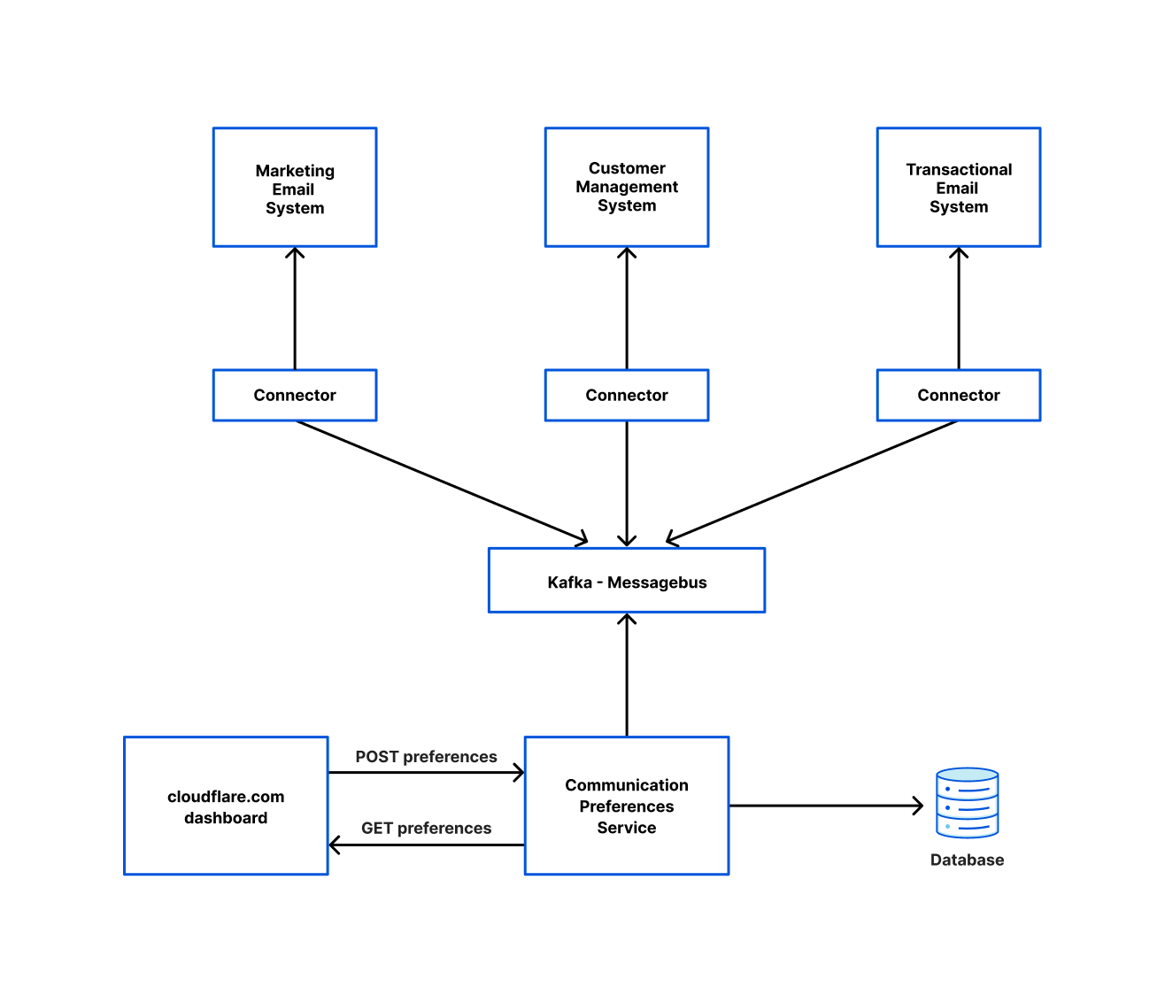
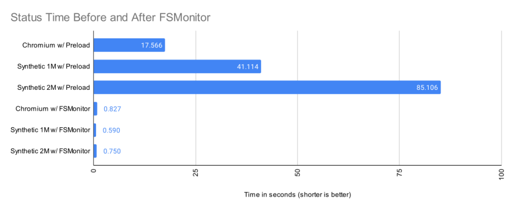
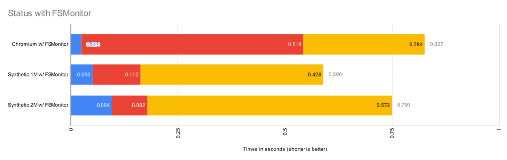
The Git file system monitor (FSMonitor) feature can speed up these commands by reducing the size of the search, and this can greatly reduce the pain of working in large worktrees. For example, this chart shows status times dropping to under a second on three different large worktrees when FSMonitor is enabled!

In this article, I want to talk about the new builtin FSMonitor git fsmonitor--daemon added in Git version 2.37.0. This is easy to set up and use since it is “in the box” and does not require any third-party tooling nor additional software. It only requires a config change to enable it. It is currently available on macOS and Windows.
To enable the new builtin FSMonitor, just set core.fsmonitor to true. A daemon will be started automatically in the background by the next Git command.
FSMonitor works well with core.untrackedcache, so we’ll also turn it on for the FSMonitor test runs. We’ll talk more about the untracked-cache later.
$ time git status
On branch main
Your branch is up to date with 'origin/main'.

It took 5.25 seconds to enumerate untracked files. 'status -uno'
may speed it up, but you have to be careful not to forget to add
new files yourself (see 'git help status').
nothing to commit, working tree clean

real    0m17.941s
user    0m0.031s
sys     0m0.046s

$ git config core.fsmonitor true
$ git config core.untrackedcache true

$ time git status
On branch main
Your branch is up to date with 'origin/main'.

It took 6.37 seconds to enumerate untracked files. 'status -uno'
may speed it up, but you have to be careful not to forget to add
new files yourself (see 'git help status').
nothing to commit, working tree clean

real    0m19.767s
user    0m0.000s
sys     0m0.078s

$ time git status
On branch main
Your branch is up to date with 'origin/main'.

nothing to commit, working tree clean

real    0m1.063s
user    0m0.000s
sys     0m0.093s

$ git fsmonitor--daemon status
fsmonitor-daemon is watching 'C:/work/chromium'
_Note that when the daemon first starts up, it needs to synchronize with the state of the index, so the next git status command may be just as slow (or slightly slower) than before, but subsequent commands should be much faster.
In this article, I’ll introduce the new builtin FSMonitor feature and explain how it improves performance on very large worktrees.
How FSMonitor improves performance
Git has a “What changed while I wasn’t looking?” problem. That is, when you run a command that operates on the worktree, such as git status, it has to discover what has changed relative to the index. It does this by searching the entire worktree. Whether you immediately run it again or run it again tomorrow, it has to rediscover all of that same information by searching again. Whether you edit zero, one, or a million files in the mean time, the next git status command has to do the same amount of work to rediscover what (if anything) has changed.
The cost of this search is relatively fixed and is based upon the number of files (and directories) present in the worktree. In a monorepo, there might be millions of files in the worktree, so this search can be very expensive.
What we really need is a way to focus on the changed files without searching the entire worktree.
How FSMonitor works
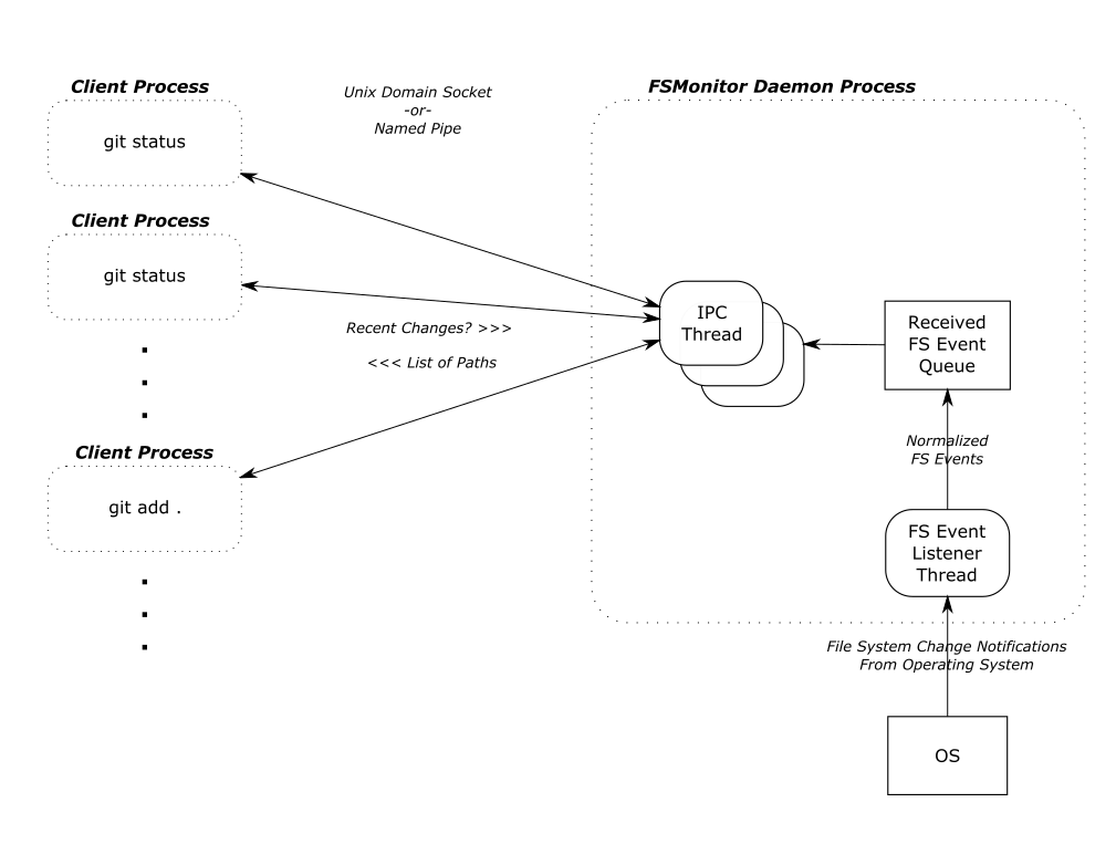
FSMonitor is a long-running daemon or service process.
- It registers with the operating system to receive change notification events on files and directories.
- It adds the pathnames of those files and directories to an in-memory, time-sorted queue.
- It listens for IPC connections from client processes, such as
git status.
- It responds to client requests for a list of files and directories that have been modified recently.

FSMonitor must continuously watch the worktree to have a complete view of all file system changes, especially ones that happen between Git commands. So it must be a long-running daemon or service process and not associated with an individual Git command instance. And thus, it cannot be a traditional Git hook (child) process. This design does allow it to service multiple (possibly concurrent) Git commands.
FSMonitor Synchronization
FSMonitor has the concept of a “token”:
- A token is an opaque string defined by FSMonitor and can be thought of as a globally unique sequence number or timestamp.
- FSMonitor creates a new token whenever file system events happen.
- FSMonitor groups file system changes into sets by these ordered tokens.
- A Git client command sends a (previously generated) token to FSMonitor to request the list of pathnames that have changed, since FSMonitor created that token.
- FSMonitor includes the current token in every response. The response contains the list of pathnames that changed between the sent and received tokens.
git status writes the received token into the index with other FSMonitor data before it exits. The next git status command reads the previous token (along with the other FSMonitor data) and asks FSMonitor what changed since the previous token.
Earlier, I said a token is like a timestamp, but it also includes other fields to prevent incomplete responses:
- The FSMonitor process id (PID): This identifies the daemon instance that created the token. If the PID in a client’s request token does not match the currently running daemon, we must assume that the client is asking for data on file system events generated before the current daemon instance was started.
- A file system synchronization id (SID): This identifies the most recent synchronization with the file system. The operating system may drop file system notification events during heavy load. The daemon itself may get overloaded, fall behind, and drop events. Either way, events were dropped, and there is a gap in our event data. When this happens, the daemon must “declare bankruptcy” and (conceptually) restart with a new SID. If the SID in a client’s request token does not match the daemon’s curent SID, we must assume that the client is asking for data spanning such a resync.
In both cases, a normal response from the daemon would be incomplete because of gaps in the data. Instead, the daemon responds with a trivial (“assume everything was changed”) response and a new token. This will cause the current Git client command to do a regular scan of the worktree (as if FSMonitor were not enabled), but let future client commands be fast again.
Types of files in your worktree
When git status examines the worktree, it looks for tracked, untracked, and ignored files.

Tracked files are files under version control. These are files that Git knows about. These are files that Git will create in your worktree when you do a git checkout. The file in the worktree may or may not match the version listed in the index. When different, we say that there is an unstaged change. (This is independent of whether the staged version matches the version referenced in the HEAD commit.)
Untracked files are just that: untracked. They are not under version control. Git does not know about them. They may be temporary files or new source files that you have not yet told Git to care about (using git add).
Ignored files are a special class of untracked files. These are usually temporary files or compiler-generated files. While Git will ignore them in commands like git add, Git will see them while searching the worktree and possibly slow it down.
Normally, git status does not print ignored files, but we’ll turn it on for this example so that we can see all four types of files.
$ git status --ignored
On branch master
Changes to be committed:
  (use "git restore --staged <file>..." to unstage)
    modified:   README

Changes not staged for commit:
  (use "git add <file>..." to update what will be committed)
  (use "git restore <file>..." to discard changes in working directory)
    modified:   README
    modified:   main.c

Untracked files:
  (use "git add <file>..." to include in what will be committed)
    new-file.c

Ignored files:
  (use "git add -f <file>..." to include in what will be committed)
    new-file.obj
The expensive worktree searches
During the worktree search, Git treats tracked and untracked files in two distinct phases. I’ll talk about each phase in detail in later sections.
- In “refresh_index,” Git looks for unstaged changes. That is, changes to tracked files that have not been staged (added) to the index. This potentially requires looking at each tracked file in the worktree and comparing its contents with the index version.
- In “untracked,” Git searches the worktree for untracked files and filters out tracked and ignored files. This potentially requires completely searching each subdirectory in the worktree.
There is a third phase where Git compares the index and the HEAD commit to look for staged changes, but this phase is very fast, because it is inspecting internal data structures that are designed for this comparision. It avoids the significant number of system calls that are required to inspect the worktree, so we won’t worry about it here.
A detailed example
The chart in the introduction showed status times before and after FSMonitor was enabled. Let’s revisit that chart and fill in some details.
I collected performance data for git status on worktrees from three large repositories. There were no modified files, and git status was clean.
- The Chromium repository contains about 400K files and 33K directories.
- A synthetic repository containing 1M files and 111K directories.
- A synthetic repository containing 2M files and 111K directories.

Here we can see that when FSMonitor is not present, the commands took from 17 to 85 seconds. However, when FSMonitor was enabled the commands took less than 1 second.
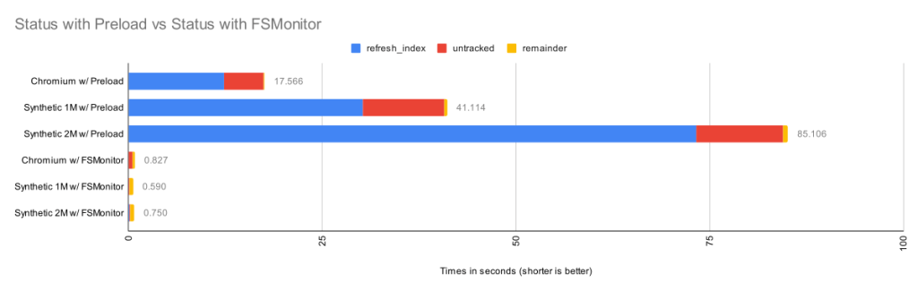
Each bar shows the total run time of the git status commands. Within each bar, the total time is divided into parts based on performance data gathered by Git’s trace2 library to highlight the important or expensive steps within the commands.
| Worktree
|
Files
|
refresh_index
with Preload
|
Untracked
without Untracked-Cache
|
Remainder
|
Total
|
| Chromium
|
393K
|
12.3s
|
5.1s
|
0.16s
|
17.6s
|
| Synthetic 1M
|
1M
|
30.2s
|
10.5s
|
0.36s
|
41.1s
|
| Synthetic 2M
|
2M
|
73.2s
|
11.2s
|
0.64s
|
85.1s
|
The top three bars are without FSMonitor. We can see that most of the time was spent in the refresh_index and untracked columns. I’ll explain what these are in a minute. In the remainder column, I’ve subtracted those two from the total run time. This portion barely shows up on these bars, so the key to speeding up git status is to attack those two phases.
The bottom three bars on the above chart have FSMonitor and the untracked-cache enabled. They show a dramatic performance improvement. On this chart these bars are barely visible, so let’s zoom in on them.
This chart rescales the FSMonitor bars by 100X. The refresh_index and untracked columns are still present but greatly reduced thanks to FSMonitor.
| Worktree
|
Files
|
refresh_index
with FSMonitor
|
Untracked
with FSMonitor
and Untracked-Cache
|
Remainder
|
Total
|
| Chromium
|
393K
|
0.024s
|
0.519s
|
0.284s
|
0.827s
|
| Synthetic 1M
|
1M
|
0.050s
|
0.112s
|
0.428s
|
0.590s
|
| Synthetic 2M
|
2M
|
0.096s
|
0.082s
|
0.572s
|
0.750s
|
This is bigger than just status
So far I’ve only talked about git status, since it is the command that we probably use the most and are always thinking about when talking about performance relative to the state and size of the worktree. But it is just one of many affected commands:
git diff does the same search, but uses the changed files it finds to print a difference in the worktree and your index.git add . does the same search, but it stages each changed file it finds.git restore and git checkout do the same search to decide the files to be replaced.
So, for simplicity, I’ll just talk about git status, but keep in mind that this approach benefits many other commands, since the cost of actually staging, overwriting, or reporting the change is relatively trivial by comparison — the real performance cost in these commands (as the above charts show) is the time it takes to simply find the changed files in the worktree.
Phase 1: refresh_index
The index contains an “index entry” with information for each tracked file. The git ls-files command can show us what that list looks like. I’ll truncate the output to only show a couple of files. In a monorepo, this list might contain millions of entries.
$ git ls-files --stage --debug
[...]
100644 7ce4f05bae8120d9fa258e854a8669f6ea9cb7b1 0   README.md
  ctime: 1646085519:36302551
  mtime: 1646085519:36302551
  dev: 16777220 ino: 180738404
  uid: 502  gid: 20
  size: 3639    flags: 0
[...]
100644 5f1623baadde79a0771e7601dcea3c8f2b989ed9 0   Makefile
  ctime: 1648154224:994917866
  mtime: 1648154224:994917866
  dev: 16777221 ino: 182328550
  uid: 502  gid: 20
  size: 110149  flags: 0
[...]
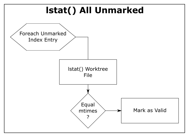
Scanning tracked files for unstaged changes
Let’s assume at the beginning of refresh_index that all index entries are “unmarked” — meaning that we don’t know yet whether or not the worktree file contains an unstaged change. And we “mark” an index entry when we know the answer (either way).

To determine if an individual tracked file has an unstaged change, it must be “scanned”. That is, Git must read, clean, hash the current contents of the file, and compare the computed hash value with the hash value stored in the index. If the hashes are the same, we mark the index entry as “valid”. If they are different, we mark it as an unstaged change.
In theory, refresh_index must repeat this for each tracked file in the index.
As you can see, each individual file that we have to scan will take time and if we have to do a “full scan”, it will be very slow, especially if we have to do it for millions of files. For example, on the Chromium worktree, when I forced a full scan it took almost an hour.
| Worktree
|
Files
|
Full Scan
|
| Chromium
|
393K
|
3072s
|
refresh_index shortcuts
Since doing a full scan of the worktree is so expensive, Git has developed various shortcuts to avoid scanning whenever possible to increase the performance of refresh_index.

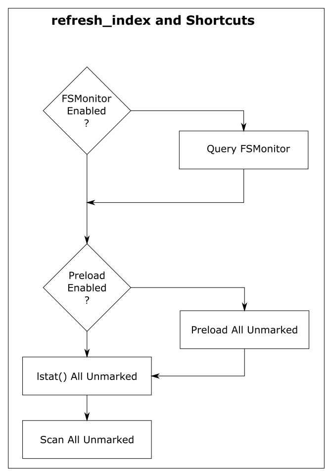
For discussion purposes, I’m going to describe them here as independent steps rather than somewhat intertwined steps. And I’m going to start from the bottom, because the goal of each shortcut is to look at unmarked index entries, mark them if they can, and make less work for the next (more expensive) step. So in a perfect world, the final “full scan” would have nothing to do, because all of the index entries have already been marked, and there are no unmarked entries remaining.

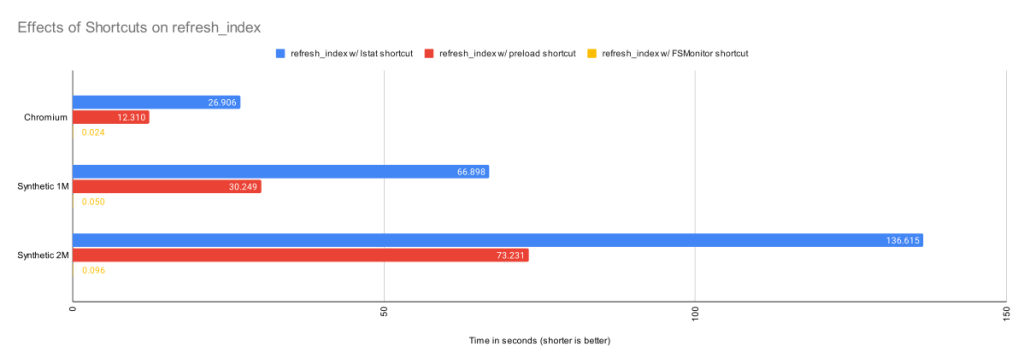
In the above chart, we can see the cummulative effects of these shortcuts.
Shortcut: refresh_index with lstat()
The “lstat() shortcut” was created very early in the Git project.
To avoid actually scanning every tracked file on every git status command, Git relies on a file’s last modification time (mtime) to tell when a file was last changed. File mtimes are updated when files are created or edited. We can read the mtime using the lstat() system call.
When Git does a git checkout or git add, it writes each worktree file’s current mtime into its index entry. These serve as the reference mtimes for future git status commands.

Then, during a later git status, Git checks the current mtime against the reference mtime (for each unmarked file). If they are identical, Git knows that the file content hasn’t changed and marks the index entry valid (so that the next step will avoid it). If the mtimes are different, this step leaves the index entry unmarked for the next step.
| Worktree
|
Files
|
refresh_index with lstat()
|
| Chromium
|
393K
|
26.9s
|
| Synthetic 1M
|
1M
|
66.9s
|
| Synthetic 2M
|
2M
|
136.6s
|
The above table shows the time in seconds taken to call lstat() on every file in the worktree. For the Chromium worktree, we’ve cut the time of refresh_index from 50 minutes to 27 seconds.
Using mtimes is much faster than always scanning each file, but Git still has to lstat() every tracked file during the search, and that can still be very slow when there are millions of files.
In this experiment, there were no modifications in the worktree, and the index was up to date, so this step marked all of the index entries as valid and the “scan all unmarked” step had nothing to do. So the time reported here is essentially just the time to call lstat() in a loop.
This is better than before, but even though we are only doing an lstat(), git status is still spending more than 26 seconds in this step. We can do better.
Shortcut: refresh_index with preload
The core.preloadindex config option is an optional feature in Git. The option was introduced in version 1.6 and was enabled by default in 2.1.0 on platforms that support threading.
This step partitions the index into equal-sized chunks and distributes it to multiple threads. Each thread does the lstat() shortcut on their partition. And like before, index entries with different mtimes are left unmarked for the next step in the process.
The preload step does not change the amount of file scanning that we need to do in the final step, it just distributes the lstat() calls across all of your cores.

| Worktree
|
Files
|
refresh_index with Preload
|
| Chromium
|
393K
|
12.3s
|
| Synthetic 1M
|
1M
|
30.2s
|
| Synthetic 2M
|
2M
|
73.2s
|
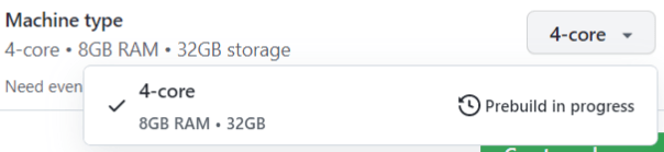
With the preload shortcut git status is about twice as fast on my 4-core Windows laptop, but it is still expensive.
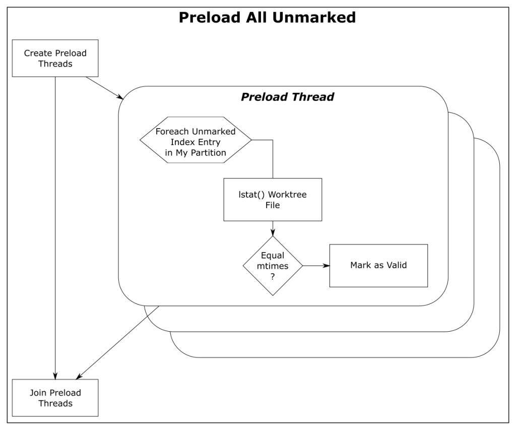
Shortcut: refresh_index with FSMonitor
When FSMonitor is enabled:
- The
git fsmonitor--daemon is started in the background and listens for file system change notification events from the operating system for files within the worktree. This includes file creations, deletions, and modifications. If the daemon gets an event for a file, that file probably has an updated mtime. Said another way, if a file mtime changes, the daemon will get an event for it.
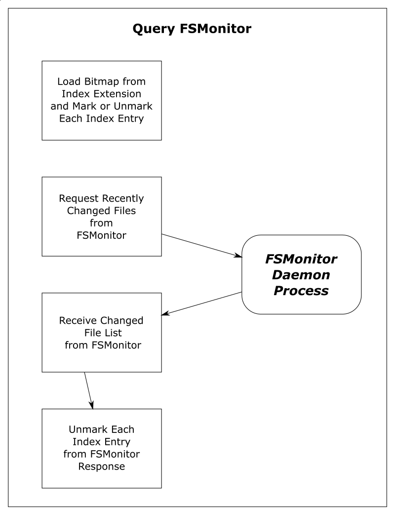
- The FSMonitor index extension is added to the index to keep track of FSMonitor and
git status data between git status commands. The extension contains an FSMonitor token and a bitmap listing the files that were marked valid by the previous git status command (and relative to that token).
- The next
git status command will use this bitmap to initialize the marked state of the index entries. That is, the previous Git command saved the marked state of the index entries in the bitmap and this command restores them — rather than initializing them all as unmarked.
- It will then ask the daemon for a list of files that have had file system events since the token and unmark each of them. FSMonitor tells us the exact set of files that have been modified in some way since the last command, so those are the only files that we should need to visit.
At this point, all of the unchanged files should be marked valid. Only files that may have changed should be unmarked. This sets up the next shortcut step to have very little to do.

| Worktree
|
Files
|
Query FSMonitor
|
refresh_index with FSMonitor
|
| Chromium
|
393K
|
0.017s
|
0.024s
|
| Synthetic 1M
|
1M
|
0.002s
|
0.050s
|
| Synthetic 2M
|
2M
|
0.002s
|
0.096s
|
This table shows that refresh_index is now very fast since we don’t need to any searching. And the time to request the list of files over IPC is well worth the complex setup.
Phase 2: untracked
The “untracked” phase is a search for anything in the worktree that Git does not know about. These are files and directories that are not under version control. This requires a full search of the worktree.
Conceptually, this looks like:
- A full recursive enumeration of every directory in the worktree.
- Build a complete list of the pathnames of every file and directory within the worktree.
- Take each found pathname and do a binary search in the index for a corresponding index entry. If one is found, the pathname can be omitted from the list, because it refers to a tracked file.
- On case insensitive systems, such as Windows and macOS, a case insensitive hash table must be constructed from the case sensitive index entries and used to lookup the pathnames instead of the binary search.
- Take each remaining pathname and apply
.gitignore pattern matching rules. If a match is found, then the pathname is an ignored file and is omitted from the list. This pattern matching can be very expensive if there are lots of rules.
- The final resulting list is the set of untracked files.
This search can be very expensive on monorepos and frequently leads to the following advice message:
$ git status
On branch main
Your branch is up to date with 'origin/main'.

It took 5.12 seconds to enumerate untracked files. 'status -uno'
may speed it up, but you have to be careful not to forget to add
new files yourself (see 'git help status').
nothing to commit, working tree clean
Normally, the complete discovery of the set of untracked files must be repeated for each command unless the [core.untrackedcache](https://git-scm.com/docs/git-config#Documentation/git-config.txt-coreuntrackedCache) feature is enabled.
The untracked-cache
The untracked-cache feature adds an extension to the index that remembers the results of the untracked search. This includes a record for each subdirectory, its mtime, and a list of the untracked files within it.
With the untracked-cache enabled, Git still needs to lstat() every directory in the worktree to confirm that the cached record is still valid.
If the mtimes match:
- Git avoids calling
opendir() and readdir() to enumerate the files within the directory,
- and just uses the existing list of untracked files from the cache record.
If the mtimes don’t match:
- Git needs to invalidate the untracked-cache entry.
- Actually open and read the directory contents.
- Call
lstat() on each file or subdirectory within the directory to determine if it is a file or directory and possibly invalidate untracked-cache entries for any subdirectories.
- Use the file pathname to do tracked file filtering.
- Use the file pathname to do ignored file filtering
- Update the list of untracked files in the untracked-cache entry.
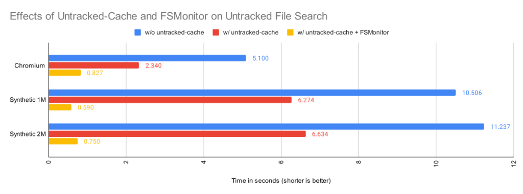
How FSMonitor helps the untracked-cache
When FSMonitor is also enabled, we can avoid the lstat() calls, because FSMonitor tells us the set of directories that may have an updated mtime, so we don’t need to search for them.

| Worktree
|
Files
|
Untracked
without Untracked-Cache
|
Untracked
with Untracked-Cache
|
Untracked
with Untracked-Cache
and FSMonitor
|
| Chromium
|
393K
|
5.1s
|
2.3s
|
0.83s
|
| Synthetic 1M
|
1M
|
10.5s
|
6.3s
|
0.59s
|
| Synthetic 2M
|
2M
|
11.2s
|
6.6s
|
0.75s
|
By itself, the untracked-cache feature gives roughly a 2X speed up in the search for untracked files. Use both the untracked-cache and FSMonitor, and we see a 10X speedup.
A note about ignored files
You can improve Git performance by not storing temporary files, such as compiler intermediate files, inside your worktree.
During the untracked search, Git first eliminates the tracked files from the candidate untracked list using the index. Git then uses the .gitignore pattern matching rules to eliminate the ignored files. Git’s performance will suffer if there are many rules and/or many temporary files.
For example, if there is a *.o for every source file and they are stored next to their source files, then every build will delete and recreate one or more object files and cause the mtime on their parent directories to change. Those mtime changes will cause git status to invalidate the corresponding untracked-cache entries and have to re-read and re-filter those directories — even if no source files actually changed. A large number of such temporary and uninteresting files can greatly affect the performance of these Git commands.
Keeping build artifacts out of your worktree is part of the philosophy of the Scalar Project. Scalar introduced Git tooling to help you keep your worktree in <repo-name>/src/ to make it easier for you to put these other files in <repo-name>/bin/ or <repo-name>/packages/, for example.
A note about sparse checkout
So far, we’ve talked about optimizations to make Git work smarter and faster on worktree-related operations by caching data in the index and in various index extensions. Future commands are faster, because they don’t have to rediscover everything and therefore can avoid repeating unnecessary or redundant work. But we can only push that so far.
The Git sparse checkout feature approaches worktree performance from another angle. With it, you can ask Git to only populate the files that you need. The parts that you don’t need are simply not present. For example, if you only need 10% of the worktree to do your work, why populate the other 90% and force Git to search through them on every command?
Sparse checkout speeds the search for unstaged changes in refresh_index because:
- Since the unneeded files are not actually present on disk, they cannot have unstaged changes. So
refresh_index can completely ignore them.
- The index entries for unneeded files are pre-marked during
git checkout with the skip-worktree bit, so they are never in an “unmarked” state. So those index entries are excluded from all of the refresh_index loops.
Sparse checkout speeds the search for untracked files because:
- Since Git doesn’t know whether a directory contains untracked files until it searches it, the search for untracked files must visit every directory present in the worktree. Sparse checkout lets us avoid creating entire sub-trees or “cones” from the worktree. So there are fewer directories to visit.
- The untracked-cache does not need to create, save, and restore untracked-cache entries for the unpopulated directories. So reading and writing the untracked-cache extension in the index is faster.
External file system monitors
So far we have only talked about Git’s builtin FSMonitor feature. Clients use the simple IPC interface to communicate directly with git fsmonitor--daemon over a Unix domain socket or named pipe.
However, Git added support for an external file system monitor in version 2.16.0 using the core.fsmonitor hook. Here, clients communicate with a proxy child helper process through the hook interface, and it communicates with an external file system monitor process.
Conceptually, both types of file system monitors are identical. They include a long-running process that listens to the file system for changes and are able to respond to client requests for a list of recently changed files and directories. The response from both are used identically to update and modify the refresh_index and untracked searches. The only difference is in how the client talks to the service or daemon.
The original hook interface was useful, because it allowed Git to work with existing off-the-shelf tools and allowed the basic concepts within Git to be proven relatively quickly, confirm correct operation, and get a quick speed up.
Hook protocol versions
The original 2.16.0 version of the hook API used protocol version 1. It was a timestamp-based query. The client would send a timestamp value, expressed as nanoseconds since January 1, 1970, and expect a list of the files that had changed since that timestamp.
Protocol version 1 has several race conditions and should not be used anymore. Protocol version 2 was added in 2.26.0 to address these problems.
Protocol version 2 is based upon opaque tokens provided by the external file system monitor process. Clients make token-based queries that are relative to a previously issued token. Instead of making absolute requests, clients ask what has changed since their last request. The format and content of the token is defined by the external file system monitor, such as Watchman, and is treated as an opaque string by Git client commands.
The hook protocol is not used by the builtin FSMonitor.
Using Watchman and the sample hook script
Watchman is a popular external file system monitor tool and a Watchman-compatible hook script is included with Git and copied into new worktrees during git init.
To enable it:
- Install Watchman on your system.
- Tell Watchman to watch your worktree:
$ watchman watch .
{
    "version": "2022.01.31.00",
    "watch": "/Users/jeffhost/work/chromium",
    "watcher": "fsevents"
}
- Install the sample hook script to teach Git how to talk to Watchman:
$ cp .git/hooks/fsmonitor-watchman.sample .git/hooks/query-watchman
- Tell Git to use the hook:
$ git config core.fsmonitor .git/hooks/query-watchman
Using Watchman with a custom hook
The hook interface is not limited to running shell or Perl scripts. The included sample hook script is just an example implementation. Engineers at Dropbox described how they were able to speed up Git with a custom hook executable.
Final Remarks
In this article, we have seen how a file system monitor can speed up commands like git status by solving the “discovery” problem and eliminating the need to search the worktree for changes in every command. This greatly reduces the pain of working with monorepos.
This feature was created in two efforts:
- First, Git was taught to work with existing off-the-shelf tools, like Watchman. This allowed the basic concepts to be proven relatively quickly. And for users who already use Watchman for other purposes, it allows Git to efficiently interoperate with them.
- Second, we brought the feature “in the box” to reduce the setup complexity and third-party dependencies, which some users may find useful. It also lets us consider adding Git-specific features that a generic monitoring tool might not want, such as understanding ignored files and omitting them from the service’s response.
Having both options available lets users choose the best solution for their needs.
Regardless of which type of file system monitor you use, it will help make your monorepos more usable.


 Structure the narrative
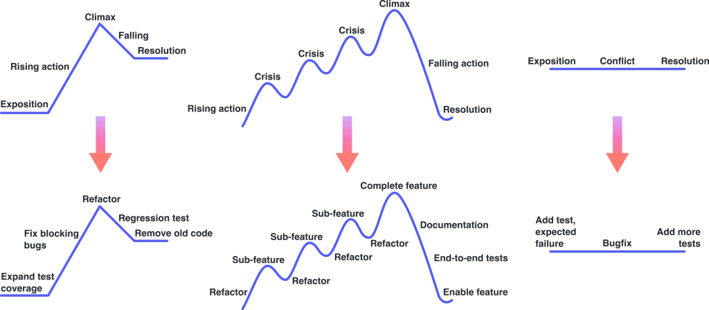
 Resize and stabilize the commits
 Explain the context


 Dependencies
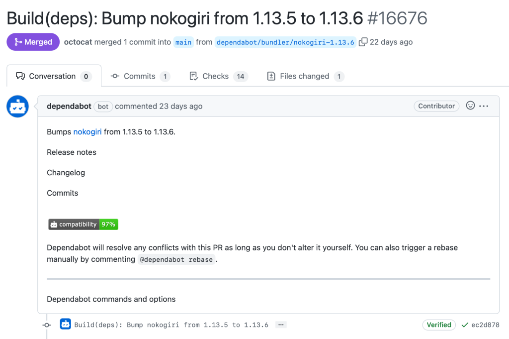


 The pitch: When it comes to what we’re going to work on (outside of the big pieces of work on
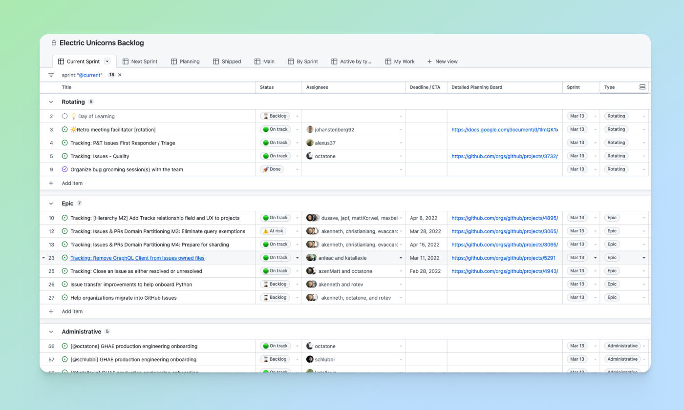
 In addition to using issues to propose and converse on pitches from the team, we use the new projects experience to track and manage all the pitches from the team so we can see them in an all-up table or board view.
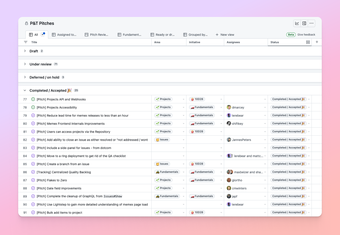
 Keep it small: We knew for ourselves, and for developers, that we didn’t want to lock them into a specific planning methodology and over-complicate a team’s planning and tracking process. For us, we wanted to plan shorter cycles for our team to increase our tempo and focus, so we opted for six-week cycles to break up and build features. Check out how we recommend getting started with this approach in a
  Ship to learn: Similar to how we ship a lot of our products, we knew developers and customers were going to be heavily intertwined with each and every ship, giving us immediate feedback in both the private and public beta. Their