Post Syndicated from The History Guy: History Deserves to Be Remembered original https://www.youtube.com/watch?v=fW5r728_Xso
Yearly Archives: 2024
Ingredients
Post Syndicated from xkcd.com original https://xkcd.com/2993/

Don’t Believe the HYPE!! FujiFilm X100VI 6 Months Later
Post Syndicated from Matt Granger original https://www.youtube.com/watch?v=FOFRkQhtl5w
THG Podcast: Hurricanes that Made History
Post Syndicated from The History Guy: History Deserves to Be Remembered original https://www.youtube.com/watch?v=ETTJoHzmixs
Accelerate Amazon Redshift Data Lake queries with AWS Glue Data Catalog Column Statistics
Post Syndicated from Kalaiselvi Kamaraj original https://aws.amazon.com/blogs/big-data/accelerate-amazon-redshift-data-lake-queries-with-column-level-statistics/
Amazon Redshift enables you to efficiently query and retrieve structured and semi-structured data from open format files in Amazon S3 data lake without having to load the data into Amazon Redshift tables. Amazon Redshift extends SQL capabilities to your data lake, enabling you to run analytical queries. Amazon Redshift supports a wide variety of tabular data formats like CSV, JSON, Parquet, ORC and open tabular formats like Apache Hudi, Linux foundation Delta Lake and Apache Iceberg.
You create Redshift external tables by defining the structure for your files, S3 location of the files and registering them as tables in an external data catalog. The external data catalog can be AWS Glue Data Catalog, the data catalog that comes with Amazon Athena, or your own Apache Hive metastore.
Over the last year, Amazon Redshift added several performance optimizations for data lake queries across multiple areas of query engine such as rewrite, planning, scan execution and consuming AWS Glue Data Catalog column statistics. To get the best performance on data lake queries with Redshift, you can use AWS Glue Data Catalog’s column statistics feature to collect statistics on Data Lake tables. For Amazon Redshift Serverless instances, you will see improved scan performance through increased parallel processing of S3 files and this happens automatically based on RPUs used.
In this post, we highlight the performance improvements we observed using industry standard TPC-DS benchmarks. Overall execution time of TPC-DS 3 TB benchmark improved by 3x. Some of the queries in our benchmark experienced up to 12x speed up.
Performance Improvements
Several performance optimizations were done over the last year to improve performance of data lake queries including the following.
- Consume AWS Glue Data Catalog column statistics and tuning of Redshift optimizer to improve quality of query plans
- Utilize bloom filters for partition columns
- Improved scan efficiency for Amazon Redshift Serverless instances through increased parallel processing of files
- Novel query rewrite rules to merge similar scans
- Faster retrieval of metadata from AWS Glue Data Catalog
To understand the performance gains, we tested the performance on the industry-standard TPC-DS benchmark using 3 TB data sets and queries which represents different customer use cases. Performance was tested on a Redshift serverless data warehouse with 128 RPU. In our testing, the dataset was stored in Amazon S3 in Parquet format and AWS Glue Data Catalog was used to manage external databases and tables. Fact tables were partitioned on the date column, and each fact table consisted of approximately 2,000 partitions. All of the tables had their row count table property, numRows, set as per the spectrum query performance guidelines.
We did a baseline run on Redshift patch version (patch 172) from last year. Later, we ran all TPC-DS queries on latest patch version (patch 180) that includes all performance optimizations added over last year. Then we used AWS Glue Data Catalog’s column statistics feature to compute statistics for all the tables and measured improvements with the presence of AWS Glue Data Catalog column statistics.
Our analysis revealed that the TPC-DS 3TB Parquet benchmark saw substantial performance gains with these optimizations. Specifically, partitioned Parquet with our latest optimizations achieved 2x faster runtimes compared to the previous implementation. Enabling AWS Glue Data Catalog column statistics further improved performance by 3x versus last year. The following graph illustrates these runtime improvements for the full benchmark (all TPC-DS queries) over the past year, including the additional boost from using AWS Glue Data Catalog column statistics.

Figure 1: Improvement in total runtime of TPC-DS 3T workload
The following graph presents the top queries from the TPC-DS benchmark with the greatest performance improvement over the last year with and without AWS Glue Data Catalog column statistics. You can see that performance improves a lot when statistics exist on AWS Glue Data Catalog (for details on how to get statistics for your Data Lake tables, please refer to optimizing query performance using AWS Glue Data Catalog column statistics). Specifically, multi-join queries will benefit the most from AWS Glue Data Catalog column statistics because the optimizer uses statistics to choose the right join order and distribution strategy.

Figure 2: Speed-up in TPC-DS queries
Let’s discuss some of the optimizations that contributed to improved query performance.
Optimizing with table-level statistics
Amazon Redshift’s design enables it to handle large-scale data challenges with superior speed and cost-efficiency. Its massively parallel processing (MPP) query engine, AI-powered query optimizer, auto-scaling capabilities, and other advanced features allow Redshift to excel at searching, aggregating, and transforming petabytes of data.
However, even the most powerful systems can experience performance degradation if they encounter anti-patterns like grossly inaccurate table statistics, such as the row count metadata.
Without this crucial metadata, Redshift’s query optimizer may be limited in the number of possible optimizations, especially those related to data distribution during query execution. This can have a significant impact on overall query performance.
To illustrate this, consider the following simple query involving an inner join between a large table with billions of rows and a small table with only a few hundred thousand rows.
If executed as-is, with the large table on the right-hand side of the join, the query will lead to sub-optimal performance. This is because the large table will need to be distributed (broadcast) to all Redshift compute nodes to perform the inner join with the small table, as shown in the following diagram.

Figure 3: Inaccurate table statistics lead to limited optimizations and large amounts of data broadcast among compute nodes for a simple inner join
Now, consider a scenario where the table statistics, such as the row count, are accurate. This allows the Amazon Redshift query optimizer to make more informed decisions, such as determining the optimal join order. In this case, the optimizer would immediately rewrite the query to have the large table on the left-hand side of the inner join, so that it is the small table that is broadcast across the Redshift compute nodes, as illustrated in the following diagram.

Figure 4: Accurate table statistics lead to high degree of optimizations and very little data broadcast among compute nodes for a simple inner join
Fortunately, Amazon Redshift automatically maintains accurate table statistics for local tables by running the ANALYZE command in the background. For external tables (data lake tables), however, AWS Glue Data Catalog column statistics are recommended for use with Amazon Redshift as we will discuss in the next section. For more general information on optimizing queries in Amazon Redshift, please refer to the documentation on factors affecting query performance, data redistribution, and Amazon Redshift best practices for designing queries.
Improvements with AWS Glue Data Catalog column statistics
AWS Glue Data Catalog has a feature to compute column level statistics for Amazon S3 backed external tables. AWS Glue Data Catalog can compute column level statistics such as NDV, Number of Nulls, Min/Max and Avg. column width for the columns without the need for additional data pipelines. Amazon Redshift cost-based optimizer utilizes these statistics to come up with better quality query plans. In addition to consuming statistics, we also made several improvements in cardinality estimations and cost tuning to get high quality query plans thereby improving query performance.
TPC-DS 3TB dataset showed 40% improvement in total query execution time when these AWS Glue Data Catalog column statistics were provided. Individual TPC-DS queries showed up to 5x improvements in query execution time. Some of the queries that had greater impact in execution time are Q85, Q64, Q75, Q78, Q94, Q16, Q04, Q24 and Q11.
We will go through an example where cost-based optimizer generated a better query plan with statistics and how it improved the execution time.
Let’s consider following simpler version of TPC-DS Q64 to showcase the query plan differences with statistics.
|
Without Statistics Following figure represents the logical query plan of Q64. You can observe that cardinality estimation of joins is not accurate. With inaccurate cardinalities, optimizer produces a sub-optimal query plan leading to higher execution time. |
With Statistics Following figure represents the logical query plan after consuming AWS Glue Data Catalog column statistics. Based on the highlighted changes, you can observe that the cardinality estimations of JOIN improved by many magnitudes helping the optimizer to choose a better join order and join strategy (broadcast |

Figure 5: Logical query plan of Q64 without statistics |

Figure 6: Logical query plan of Q64 after consuming AWS Glue Data Catalog column statistics |
This change in query plan improved the query execution time of Q64 from 383s to 81s.
Given the greater benefits with AWS Glue Data Catalog column statistics for the optimizer, you should consider collecting stats for your data lake using AWS Glue. If your workload is a JOIN heavy workload, then collecting stats will show greater improvement on your workload. Refer to generating AWS Glue Data Catalog column statistics for instructions on how to collect statistics in AWS Glue Data Catalog.
Query rewrite optimization
We introduced a new query rewrite rule which combines scalar aggregates over the same common expression using slightly different predicates. This rewrite resulted in performance improvements on TPC-DS queries Q09, Q28, and Q88. Let’s focus on Q09 as a representative of these queries, given by the following fragment:
In total, there are 15 scans of the fact table store_sales, each one returning various aggregates over different subsets of data. The engine first performs subquery removal and transforms the various expressions in the CASE statements into relational subtrees connected via cross products, and then they are fused into one subquery handling all scalar aggregates. The resulting plan for Q09, described below using SQL for clarity, is given by:
In general, this rewrite rule results in the largest improvements both in latency (from 3x to 8x improvements) and bytes read from Amazon S3 (from 6x to 8x reduction in scanned bytes and, consequently, cost).
Bloom filter for partition columns
Amazon Redshift already uses Bloom filters on data columns of external tables in Amazon S3 to enable early and effective data filtering. Last year, we extended this support for partition columns as well. A Bloom filter is a probabilistic, memory-efficient data structure that accelerates join queries at scale by filtering rows that do not match the join relation, significantly reducing the amount of data transferred over the network. Amazon Redshift automatically determines what queries are suitable for leveraging Bloom filters at query runtime.
This optimization resulted in performance improvements on TPC-DS queries Q05, Q17 and Q54. This optimization resulted in large improvements in both latency (from 2x to 3x improvement) and bytes read from S3 (from 9x to 15x reduction in scanned bytes and, consequently cost).
Following is the subquery of Q05 which showcased improvements with runtime filter.
|
Without bloom filter support on partition columns Following figure is the logical query plan for sub-query of Q05. This appends two large fact tables |
With bloom filter support on partition columns With support of bloom filter on partition columns, we now create bloom filter for |

Figure 7: Logical query plan for sub-query of Q05 without bloom filter support on partition columns |

Figure 8: Logical query plan for sub-query of Q05 with bloom filter support on partition columns |
Overall, bloom filter on partition column will reduce the number of partitions processed resulting in reduced S3 listing calls and lesser number of data files to be read (reduction in scanned bytes). You can see that we only scan 89M rows from store_sales and 4M rows from store_returns because of the bloom filter. This reduced number of rows to process at JOIN level and helped in improving the overall query performance by 2x and scanned bytes by 9x.
Conclusion
In this post, we covered new performance optimizations in Amazon Redshift data lake query processing and how AWS Glue Data Catalog statistics helps to enhance quality of query plans for data lake queries in Amazon Redshift. These optimizations together improved TPC-DS 3 TB benchmark by 3x. Some of the queries in our benchmark benefited up to 12x speed up.
In summary, Amazon Redshift now offers enhanced query performance with optimizations such as AWS Glue Data Catalog column statistics, bloom filters on partition columns, new query rewrite rules and faster retrieval of metadata. These optimizations are enabled by default and Amazon Redshift users will benefit with better query response times for their workloads. For more information, please reach out to your AWS technical account manager or AWS account solutions architect. They will be happy to provide additional guidance and support.
About the authors
 Kalaiselvi Kamaraj is a Sr. Software Development Engineer with Amazon. She has worked on several projects within Redshift Query processing team and currently focusing on performance related projects for Redshift Data Lake.
 Mark Lyons is a Principal Product Manager on the Amazon Redshift team. He works on the intersection of data lakes and data warehouses. Prior to joining AWS, Mark held product leadership roles with Dremio and Vertica. He is passionate about data analytics and empowering customers to change the world with their data.
 Asser Moustafa is a Principal Worldwide Specialist Solutions Architect at AWS, based in Dallas, Texas, USA. He partners with customers worldwide, advising them on all aspects of their data architectures, migrations, and strategic data visions to help organizations adopt cloud-based solutions, maximize the value of their data assets, modernize legacy infrastructures, and implement cutting-edge capabilities like machine learning and advanced analytics. Prior to joining AWS, Asser held various data and analytics leadership roles, completing an MBA from New York University and an MS in Computer Science from Columbia University in New York. He is passionate about empowering organizations to become truly data-driven and unlock the transformative potential of their data.
How to perform a proof of concept for automated discovery using Amazon Macie
Post Syndicated from Jason Stone original https://aws.amazon.com/blogs/security/proof-of-concept-for-automated-discovery-using-amazon-macie/
Amazon Web Services (AWS) customers of various sizes across different industries are pursuing initiatives to better classify and protect the data they store in Amazon Simple Storage Service (Amazon S3). Amazon Macie helps customers identify, discover, monitor, and protect sensitive data stored in Amazon S3. However, it’s important that customers evaluate and test the capabilities of Macie to verify that they can meet their specific data identification and protection goals. In this post, we show you how to define and run a proof of concept (POC) to validate using Macie and automated discovery to enhance your current data protection strategies. The POC steps demonstrate how you can use Macie to detect and alert you to sensitive data discovered in your AWS environment and help you determine the value of using Macie to enhance your current data protection strategies.
Note: This POC uses some features that offer a 30-day free trial and other features that will incur minimal charges during the POC phase. We highlight and summarize these throughout this post.
Data security business challenges
Data security is a broad concept that revolves around protecting digital information from unauthorized access, corruption, theft, and other forms of malicious activity throughout its lifecycle. There’s an exponential growth of digital data and organizations are grappling with not only managing it but also determining where their sensitive data exists. Additionally, many organizations have compliance requirements from government regulators and industry standards, such as PCI DSS or HIPAA. Organizations want to move fast, which means giving developers the tools to build quickly to stay ahead, while making sure that the correct data classification policies are defined and enforced.
Macie features
Amazon Macie is a data security service that discovers sensitive data using machine learning and pattern matching, provides visibility into data security risks, and enables automated protection against those risks. The following is a summary of the key features of Macie, many of which will be used in this POC. The core capabilities of Macie are focused on the security of your S3 buckets and helping to identify sensitive data including financial data, personal data, and credentials as well as sensitive data that’s unique to your organization, such as intellectual property.
S3 bucket security
Customers use Amazon S3 for a variety of use cases and store various types of data in S3 buckets, including sensitive data. Continuously monitoring these buckets for the presence of sensitive data is a vital part of a data protection strategy. Macie gives you visibility into your S3 bucket inventory and the security and access controls associated with your buckets. This visibility includes if the bucket is publicly accessible, the encryption level of the bucket, and if the bucket is shared with other accounts. Whenever the security posture of one of your buckets is reduced, Macie generates a finding about the change, enabling you to respond. These findings are consumable through the AWS Management Console for Macie, through Macie APIs, as Amazon EventBridge messages, or through AWS Security Hub.
Sensitive data discovery jobs
Sensitive data discovery jobs provide a way to target a specific S3 bucket or group of buckets to do a deep analysis of the objects in those buckets and identify if sensitive data is present in the objects and if so, the type of data. These jobs can run on a daily, weekly, or monthly basis for new or changed data or once for on-demand analysis.
Automated data discovery
Macie offers an automated data discovery feature that can continually discover sensitive data within your S3 buckets. This feature is intended to help customers who have large amounts of S3 buckets and data better understand where sensitive data might be stored without having to scan all their data. By using automated data discovery, you can focus your resources on deeper investigations of the security of buckets identified to have sensitive data. Macie selects samples of the objects within S3 buckets and inspects them for the presence of sensitive data daily, providing insight into where sensitive data might reside in your overall Amazon S3 data estate.
POC overview
This POC is intended to help you gain an understanding of what Macie is capable of and how you can use it to achieve your data discovery goals. The POC in this post includes the following tasks in Macie:
- Reviewing managed data identifiers
- Defining custom data identifiers
- Staging POC data
- Running a sensitive data discovery job
- Reviewing the output of the discovery job
- Enabling and reviewing the output of automated data discovery
Note: The amount of time required for each task depends on your preparation and analysis for each stage. Note that, in the automated data discovery phase, it will take 24–48 hours for Macie to perform the first scan after the feature is enabled.
Enable Macie
Macie must be enabled before you can proceed with the POC. If you haven’t yet enabled Macie, see Enable Macie for instructions.
Note: When you enable Macie and the 30-day free trial for S3, monitoring S3 bucket security and privacy is automatically enabled. There’s also a 30-day free trial for automated data discovery, which is covered later in this post. There is no free trial for running targeted data discovery jobs. Review the Macie pricing page for details.
Review managed data identifiers
A successful POC of Macie includes understanding what data Macie can detect. Macie comes with over 150 managed data identifiers that are designed to identify sensitive data in your S3 objects. It’s important to first understand the available managed data identifiers and which ones align with the use cases you want to address. Examples of Macie managed data identifiers include credit card numbers, AWS secret access keys, and national identification numbers. Macie offers a default collection of recommend managed data identifiers to use for detecting general categories and types of sensitive data while optimizing data discovery results and reducing noise.
Keywords are an important component for Macie to be able to detect sensitive data. Many managed data identifiers require keywords to be in proximity of the data for Macie to be able to detect findings. Understanding the keywords that are used as part of sensitive data detection is important when it comes to building test data for a POC.
Prior to beginning your POC, review the list of managed data identifiers and determine which ones you feel will be necessary to use for your data discovery requirements. Additionally, identify which managed data identifiers, which are applicable to your POC, fall outside of the default list of identifiers.
Define custom data identifiers
Macie covers a wide number of use cases with its managed data identifiers, but some use cases need custom data identifiers for data types that aren’t included in the managed data identifiers. For example, customers might need to identify sensitive data that’s specific to their company, such as an employee ID or project number. Other customers might operate in industries that have data types unique to that industry, such as a known traveler number in the airline industry. If your requirements for identifying sensitive data include detecting sensitive data that isn’t part of the current list of managed data identifiers, then you can create custom data identifiers for those data types. For a POC, you might not want to create a custom data identifier for every additional detection. Instead, you can create a few to help confirm that you can use custom data identifiers for sensitive data detection and that Macie can support your data discovery goals. Building custom data identifiers has a thorough explanation of how to define a custom data identifier. Similar to managed data identifiers, custom data identifiers have keyword requirements. Defining detection criteria for custom data identifiers provides details for the types of data that require keywords.
Stage POC data
After reviewing the managed data identifiers provided by Macie and creating the custom data identifiers needed for your POC, it’s time to stage data sets that will help demonstrate the capabilities of these identifiers and better understand how Macie identifies sensitive data. We recommend that you stage data sets that contain sensitive data as well as data sets that do not to gain a full understanding of how Macie detects and reports on each of these situations. You can stage a variety of data sets to use for your POC using just a few GB of data to help keep your initial POC scans’ cost low. Staged data must be in file formats that Macie supports.
When preparing data to stage, keep in mind the keyword requirements for many of the Macie managed data identifiers. To determine which managed data identifiers have keyword requirements, see Managed data identifiers by type. When you’re staging your data, reference the keywords that are supported for the managed data identifiers you are using to help ensure that the data can be identified in your POC tests.
We recommend staging the data in one S3 bucket that’s dedicated to the POC and to use S3 server-side encryption on the bucket. If you want to use a customer managed AWS KMS key to encrypt the S3 data at rest, follow the instructions in Allowing Macie to use a customer managed AWS KMS key to give Macie access to decrypt the data in the bucket. You should also follow best practices for the S3 bucket related to not allowing public access and implementing least privilege access.
You can use one or more of the following approaches to identify and stage data for your POC:
- Stage data files created by synthetic data generator tools with sensitive data included. There are many tools available for generating sensitive data. The following are two that you can use to generate test data.
- Stage data files from public data repositories. There are various repositories staged with information that could be used for sensitive data detection. These repositories are often comprised of publicly available data sets or were created to help with testing machine learning models or sensitive data detection.
- Stage data files of your own data with sensitive information. Because the goal is to use Macie to identify sensitive information in your S3 buckets, including examples of your own data that contains sensitive information can be helpful to test the capabilities of Macie.
- Stage data files that don’t contain sensitive information. This can help you understand how Macie handles data that you believe doesn’t contain sensitive information. With the managed data identifiers that Macie offers, you should stage data files that you believe don’t contain information that aligns to the managed data identifiers. The staged data files could be log files, documents, or data sets that meet the criteria of this step.
- Stage data that contains information that’s representative of data that you would want to detect using custom data identifiers.
Run a data classification job
Now that you’ve reviewed the managed data identifiers, defined custom data identifiers, and staged sample data, it’s time to run a sensitive data discovery job. When configuring the job scope, we recommend the following:
- A specific S3 bucket where the POC data is staged.
- The scope is set to be a one-time job.
- Leave the sampling depth at 100 percent. Most customers leave this value at 100 percent, but some will lower it if they want a smaller random sample scan of their data. Most customers use automated data discovery to get sample scans instead of adjusting the sampling depth for individual jobs.
- Select the recommended managed data identifiers. If your testing requires that Macie identify additional sensitive data types that are offered as managed data identifiers but aren’t part of the recommended list, choose the Custom option and select the managed data identifiers that you need. Make sure that the recommended managed data identifiers are part of the custom list that you construct.
- Choose the custom data identifiers that you want to be used in the job.
After you configure your job, give it a name, review the final configuration, and then submit the job to run. A job that uses a data set of a few GB should complete within 30 minutes.
Review the findings from your job
After the job completes, it’s time to review what Macie found in the data. Objects that Macie found with sensitive data will be presented as Findings in the Macie console. From the Jobs screen, choose the job you submitted. In the right-hand window, you will see the overview information for the job. From the overview window you can choose Show results menu and then select Show findings to view a list of the findings that were generated by the job.
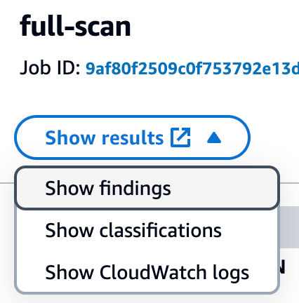
Figure 1: Viewing Macie job findings
Each object where Macie found sensitive data will be listed as a single finding. If there were multiple types of sensitive data found in the object, each type of sensitive data and a count will be included in the details. Choose each of the findings that was produced and review the details to confirm what sensitive data was identified and if the sensitive data was discovered as you expected. Additionally, confirm that you don’t have findings for objects that you staged that were not supposed to have sensitive data so that you can confirm how Macie handles these types of objects. If you created custom data identifiers, review findings for the objects that included the custom data that you detect to confirm that the data was detected.
Enable automated discovery
Now that you understand how to use Macie to discover sensitive data, the next step in the POC is to enable automated discovery and use Macie to discover sensitive data across a larger collection of your existing S3 data.
You will be enabling automated discovery in Macie as a 30-day free trial. For the free trial, the scope of total data storage to be evaluated will be 150 GB. Use the following steps to guide your setup of the automated discovery feature:
- To use automated discovery, ensure that you have a delegated administrator account defined for Macie. See Integrating and configuring an organization in Macie for steps on how to configure your delegated administrator account for Macie.
- After your delegated administrator account is configured, enable automated discovery. As part of enabling automated discovery, pay extra attention to the following items:
- Set managed data identifiers. Ideally, choose the recommended data identifiers to help reduce noise. If there are specific managed data identifiers that you really want to see, then choose Custom to choose the ones you want.
- Include custom data identifiers that you want to be used to evaluate your sensitive data.
- Exclude buckets that you don’t want included in the scope for identifying sensitive data.
- Include or exclude specific accounts that should be part of the POC. Step 5 of Enable automated discovery covers how to enable it for specific accounts.
You will see the first set of results 24 to 48 hours after you enable automated discovery. After that, you will see updates to the automated discovery results every 24 hours.
After automated discovery starts producing results, you will start seeing data in the Automated Discovery section of the Macie summary page in the console. The summary includes metrics for the total number of buckets eligible for discovery, counts for the number of buckets where sensitive data was or was not found, and how many of these buckets are public.
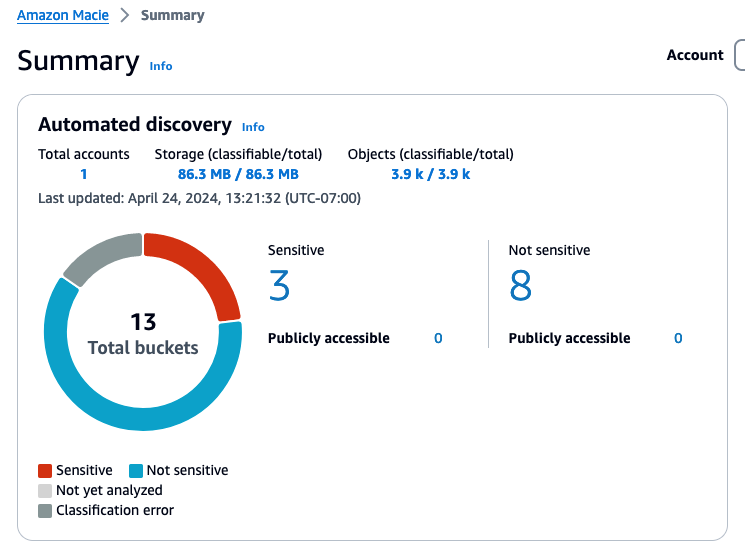
Figure 2: Example automated discovery summary metrics
Choosing a link for one of the counts will take you to the S3 buckets view with the appropriate filters applied.
After reviewing the summary screen, choose S3 buckets from the navigation pane to see a heatmap that shows each account and the buckets within each account.
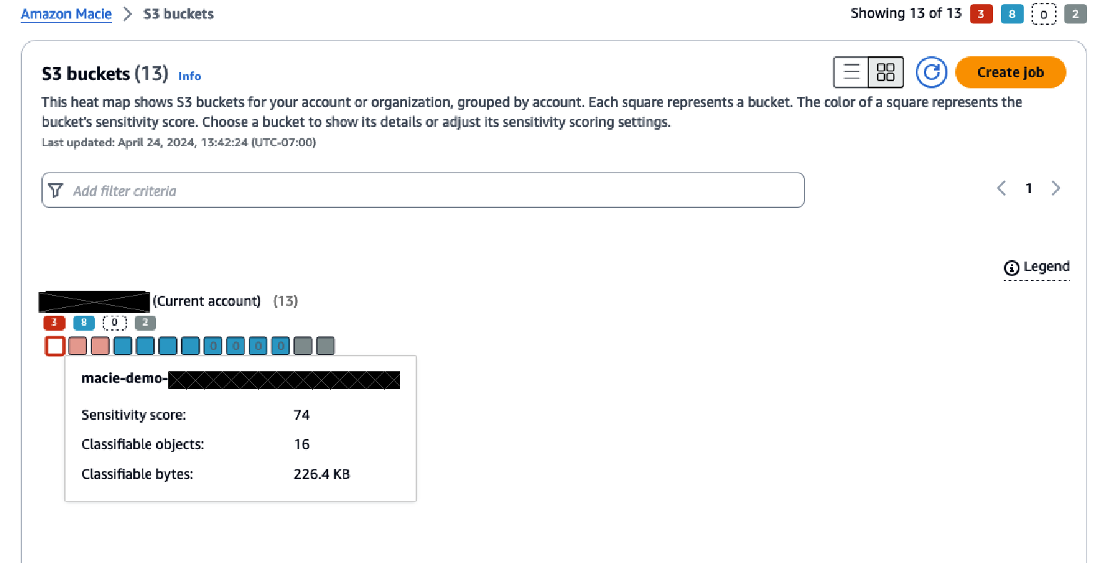
Figure 3: S3 bucket heatmap view in Macie
The heatmap provides point-in-time insights into the data that Macie has scanned, and in which buckets sensitive data has been identified or no sensitive data has been found.
Over time, this heatmap might change as automated data discovery continues sampling the data in each bucket. The heatmap view provides information on each organizational member account and insight about sensitive data within each bucket in the account.
The console displays the results as a set of colored squares for each account. Each square represents a bucket in that account and the color of the square indicates whether sensitive data was discovered in that bucket. Red indicates that some type of sensitive data has been found in the bucket, while blue indicates no sensitive data has been identified. If a bucket is blue, that means only that automated data discovery hasn’t identified sensitive data up to the point in time of the last scan, not that there is no sensitive data in the bucket.
Hover over each bucket to see a summary of the sensitivity score of the bucket along with statistics about the data in the bucket. Choosing a bucket in the heatmap will open a window that provides more information about the bucket. This information includes the sensitivity score of the bucket, a summary of the types of sensitive data found in the bucket, which objects within the bucket have been sampled, statistics related to the data that has been scanned and data that is still to be scanned, and other information about the bucket.
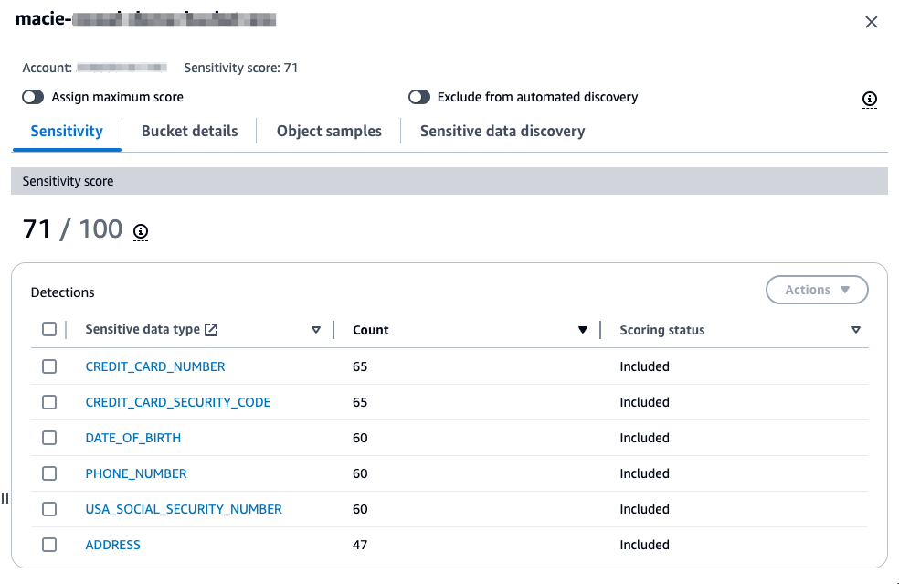
Figure 4: S3 bucket sensitivity information in Macie
As part of your POC, it’s recommended that you investigate buckets that are reported to contain sensitive data. For your investigation, validate if the data identified is sensitive based on your organization’s data classification policy. Each Macie finding contains not only the details on the types of sensitive data identified, but also the location within the file where the sensitive data is located so that you can confirm the identified data is sensitive. The following is an example of a Macie finding in an Excel file where bank account numbers were found. This example shows the row and column where the sensitive data was found.
Investigating sensitive data with findings has detailed guidance around locating sensitive data from Macie findings, retrieving the sensitive data, and the schema for sensitive data locations. If the findings are true positives, make sure that the bucket has the right level of security configurations and permissions based on the data stored in the bucket.
In addition to reviewing the bucket level statistics that are generated by automated discovery, you can view the individual findings that were generated for each S3 object that was identified as having sensitive data. You can view the findings through the Findings tab in Macie or by choosing the sensitive data type when looking at the summary detections for a bucket.
Next steps
With the preceding POC, you should now have a more complete understanding of how Macie identifies sensitive data and how you can use the information that Macie provides about that data identified. As you complete your POC, there are a few next steps that other customers have taken after completing their POC with Macie.
Operationalize Macie output
In the POC steps, we outlined how to view the findings and the insights that the automated discovery provides. Before you proceed with Macie, you should have a plan for how you will operationalize the Macie output. This will help ensure that the remediation steps for identified sensitive data are directed to the correct parties.
Depending on what operational tools you have in place, the steps that you take to operationalize the output of Macie will vary. Many customers implement operational processes that cover the following areas:
- The privacy or security team that’s responsible for Macie does an initial triage on the findings to confirm if there are true positives.
- The privacy or security team defines their operational processes related to the summary dashboard and bucket sensitivity information that’s provided by automated discovery.
- The team that owns the bucket where the sensitive data is located is provided the information needed to investigate the identified data and provide a response. Responses will vary but could include removal of the data, correcting the application that is writing the data, or applying additional security to the bucket.
A key part of operationalizing Macie output is also how you are getting and reviewing the signals related to Macie findings. As outlined in this post, you can view and investigate findings in the Macie console. At a steady state, customers find it beneficial to consume Macie findings using Amazon EventBridge, through Macie APIs, or through the integration of Macie with AWS Security Hub. These options can be used to incorporate the findings that are reported by Macie into the operational workflows and tools that work best for your organization and allow you to consume and address findings at scale. Monitoring and processing findings provides more insight into these integration approaches.
Store and retain sensitive data discovery results
As you move forward with Macie, it’s important to enable logging for each of the S3 objects that Macie has scanned. Macie creates an analysis record for each S3 object that’s in scope for a data discovery job or an automated discovery scan. These records are an audit of every object that Macie attempted to scan, including objects that didn’t contain sensitive data. Data discovery results are written to an S3 bucket that you own and where you control the data retention. These data discovery results can assist with analysis of records over time or to get a broader sense of what data Macie has scanned and which objects had sensitive data and which did not.
The data discovery scan results are stored as JSON Lines files. You can use multiple approaches to analyze and query these log files. The Amazon Macie Results Analytics GitHub repository provides instructions on how to configure Amazon Athena with tables that allow you to query the results of Macie discovery scan files.
Define the scope for Macie use
After a POC with Macie, you can set the scope of how you will use Macie in production by deciding which buckets don’t need to be evaluated and so can be excluded, such as buckets used for AWS logs and buckets deemed not in scope for sensitive data identification.
You can also refine the managed data identifiers that are required for detecting sensitive data. Based on what they learned from the POC. You can create custom data identifiers to help meet your data detection needs if necessary.
As you identify the sensitive data discovery jobs to run as part of your production use of Macie, keep in mind that these jobs are immutable. To edit an existing scheduled job, you must create a copy of the job with the updated configuration and cancel the original job for changes to take effect. Depending on the updated criteria for your job, you must do one of the following to help avoid re-scanning objects that were covered by the previous job:
- Clear include existing objects when setting the scope. This will cause the new job to schedule only objects that were created between when it was first created and when it was run for the first time.
- When setting the job scope, set the object attributes so that the object last modified date is the date of the last time the previous job ran. This helps ensure that when the new scheduled job runs, it evaluates only objects that weren’t covered by the previous job.
Clean up
To avoid incurring additional charges, disable Macie while you evaluate the value of the additional data protection provided. If S3 buckets were created for this POC, those should also be deleted.
Call to action
After the POC is complete, evaluate the results to determine how much using Macie can strengthen your organization’s data protection program. Based on that evaluation, you can identify how and where to use Macie for maximum effectiveness. Also consider how the information provided can be factored into operational workflows to get additional value from Macie.
Conclusion
This post outlined how you can use a POC to better understand how Amazon Macie can help meet your data discovery and classification needs. A well thought-out and implemented POC can provide valuable early insights and help you develop a more thorough understanding of what your data discovery and classification strategy should be. Planning your POC using the guidance in this post can help you determine more quickly if Macie is a fit for your company.
If you have feedback about this post, submit comments in the Comments section below. If you have questions about this post, contact AWS Support.
Tightrope walking, aka Funambulism
Post Syndicated from The History Guy: History Deserves to Be Remembered original https://www.youtube.com/watch?v=uqY-T8SV-rk
NICE DCV is now Amazon DCV with 2024.0 release
Post Syndicated from Sébastien Stormacq original https://aws.amazon.com/blogs/aws/nice-desktop-cloud-visualization-dcv-is-now-amazon-dcv/
Today, NICE DCV has a new name. So long NICE DCV, welcome Amazon DCV. Today, with the 2024.0 release, along with enhancements and bug fixes, NICE DCV is rebranded to Amazon DCV.
The new name is now also used to consistently refer to the DCV protocol powering AWS managed services such as Amazon AppStream 2.0 and Amazon WorkSpaces.
What is Amazon DCV
Amazon DCV is a high-performance remote display protocol. It lets you securely deliver remote desktops and application streaming from any cloud or data center to any device, over varying network conditions. By using Amazon DCV with Amazon Elastic Compute Cloud (Amazon EC2), you can run graphics-intensive applications remotely on EC2 instances. You can then stream the results to more modest client machines, which eliminates the need for expensive dedicated workstations.
Amazon DCV supports both Windows and major flavors of Linux operating systems on the server side, providing you flexibility to fit your organization’s needs. The client-side that receives the desktops and application streamings could be the native DCV client for Windows, Linux, or macOS or web browsers. The DCV remote server and client transfer only encrypted pixels, not data, so no confidential data is downloaded from the DCV server. When you choose to use Amazon DCV on Amazon Web Services (AWS) with EC2 instances, you can take advantage of the AWS 108 Availability Zones across the 33 geographic Regions and 31 local zones, allowing your remote streaming services to scale globally.
Since Amazon acquired NICE 8 years ago, we’ve witnessed a diverse range of customers adopting DCV. From general-purpose users visualizing business applications to industry-specific professionals, DCV has proven to be versatile. For instance, artists have employed DCV to access powerful cloud workstations for their digital content creation and rendering tasks. In the healthcare sector, medical imaging professionals have used DCV for remote visualization and analysis of patient data. Geoscientists have used DCV to analyze reservoir simulation results, while engineers in manufacturing have used it to visualize computational fluid dynamics experiments. The education and IT support industries have benefited from collaborative sessions in DCV, in which multiple users can share a single desktop.
Notable customers include Quantic Dream, an award-winning game development studio that has harnessed DCV to create high-resolution, low-latency streaming services for their artists and developers. Tally Solutions, an enterprise resource planning (ERP) services provider, has employed DCV to securely stream its ERP software to thousands of customers. Volkswagen has used DCV to provide remote access to computer-aided engineering (CAE) applications for over 1,000 automotive engineers. Amazon Kuiper, an initiative to bring broadband connectivity to underserved communities, has used DCV for designing complex chips.
Within AWS, DCV has been adopted by several services to provide managed solutions to customers. For example, AppStream 2.0 uses DCV to offer secure, reliable, and scalable application streaming. Additionally, since 2020, Amazon WorkSpaces Streaming Protocol (WSP), which is built on DCV and optimized for high performance, is available for Amazon WorkSpaces customers. Today, we’re also phasing out the WSP name and replacing it with DCV. Going forward, you will have DCV as a primary protocol choice in Amazon WorkSpaces.
What’s new with version 2024.0
Amazon DCV 2024.0 introduces several fixes and enhancements for improved performance, security, and ease of use. The 2024.0 release now supports the latest Ubuntu 24.04 LTS, bringing the latest security updates and extended long-term support to simplify system maintenance. The DCV client on Ubuntu 24.04 has built in support for Wayland, offering better graphical rendering efficiency and enhanced application isolation. Additionally, DCV 2024.0 now enables the QUIC UDP protocol by default, allowing clients to benefit from an optimized streaming experience. The release also introduces the capability to blank the Linux host screen when a remote user is connected, preventing local access and interaction with the remote session.
How to get started
The easiest way to test DCV is to spin up a WorkSpaces instance from the WorkSpaces console, selecting one of the DCV-powered bundles, or creating an AppStream session. For this demo however, I want to show you how to install DCV server on an EC2 instance.
I installed DCV server on two servers running on Amazon EC2, one running Windows Server 2022 and one running Ubuntu 24.04. I also installed the client on my macOS laptop. The client and server packages are available to download on our website. For both servers, make sure the security group authorizes inbound connection on UDP or TCP port 8443, the default port DCV uses.
The Windows installation is straightforward: start the msi file, select Next at each step and voilà. It was installed in less time than it took me to write this sentence.
The installation on Linux deserves a bit more care. Amazon Machine Images (AMI) for EC2 servers don’t include any desktop or graphical components. As a prerequisite, I had to install the X Window System and a window manager, and configure X to let users connect and start a graphical user interface session on the server. Fortunately, all these steps are well documented. Here is a summary of the commands I used.
# install desktop packages
$ sudo apt install ubuntu-desktop

# install a desktop manager
$ sudo apt install gdm3

# reboot
$ sudo reboot
After the reboot, I installed the DCV server package
# Install the server
$ sudo apt install ./nice-dcv-server_2024.0.17794-1_amd64.ubuntu2404.deb
$ sudo apt install ./nice-xdcv_2024.0.625-1_amd64.ubuntu2404.deb

# (optional) install the DCV web viewer to allow clients to connect from a web browser
$ sudo apt install ./nice-dcv-web-viewer_2024.0.17794-1_amd64.ubuntu2404.deb
Because my server had no GPU, I also followed these steps to install X11 Dummy driver and configure X11 to use it.
Then, I started the service:
$ sudo systemctl enable dcvserver.service
$ sudo systemctl start dcvserver.service
$ sudo systemctl status dcvserver.service
I created a user at the operating system level and assigned a password and a home directory. Then, I checked my setup on the server before trying to connect from the server.
$ sudo dcv list-sessions
There are no sessions available.

$ sudo dcv create-session console --type virtual --owner seb

$ sudo dcv list-sessions
Session: 'console' (owner:seb type:virtual)
Once my server configuration was ready, I started the DCV client on my laptop. I only had to enter the IP address of the server and the username and password of the user to initiate a session.
 |
 |
On my laptop, I opened a new DCV client window and connected to the other EC2 server. After a few seconds, I was able to remotely work with the Windows and the Ubuntu machine running in the cloud.

In this example, I focus on installing Amazon DCV on a single EC2 instance. However, when building your own service infrastructure, you may want to explore the other components that are part of the DCV offering: Amazon DCV Session Manager, Amazon DCV Access Console, and Amazon DCV Connection Gateway.
Pricing and availability
Amazon DCV is free of charges when used on AWS. You only pay for the usage of AWS resources or services, such as EC2 instances, Amazon Workspace desktops, or Amazon App Stream 2.0. If you plan to use DCV with on-premises servers, check the list of license resellers on our website.
BIG NEWS!!
Post Syndicated from Matt Granger original https://www.youtube.com/watch?v=Q0L5fmr-nFs
FFmpeg 7.1 released
Post Syndicated from jzb original https://lwn.net/Articles/992496/
Version 7.1 of
the FFmpeg audio/video toolkit has been released. Important changes in
this release include the VVC decoder reaching stable status, and
inclusion of support for MV-HEVC decoding (which is generated by
recent phones and VR headsets), as well as support for Vulkan encoding
with H264 and HEVC. See the announcement and changelog
for full details.
Firefox 131.0 released
Post Syndicated from corbet original https://lwn.net/Articles/992489/
Version
131.0 of the Firefox browser has been released. Changes include the
ability to temporarily grant permissions to sites and a preview that pops
up when hovering over tabs.
AMD EPYC Embedded 8004 Series Launches with a New 70W SKU
Post Syndicated from Cliff Robinson original https://www.servethehome.com/amd-epyc-embedded-8004-series-launches-with-a-new-70w-sku/
The new AMD EPYC Embedded 8004 series includes a new 12-core SKU with cTDP as low as 70W making for a really neat embedded part
The post AMD EPYC Embedded 8004 Series Launches with a New 70W SKU appeared first on ServeTheHome.
Social health expert on the evolution of understanding health
Post Syndicated from Talks at Google original https://www.youtube.com/watch?v=M7XarcYWBME
Keep your firewall rules up-to-date with Network Firewall features
Post Syndicated from Salman Ahmed original https://aws.amazon.com/blogs/security/keep-your-firewall-rules-up-to-date-with-network-firewall-features/
AWS Network Firewall is a managed firewall service that makes it simple to deploy essential network protections for your virtual private clouds (VPCs) on AWS. Network Firewall automatically scales with your traffic, and you can define firewall rules that provide fine-grained control over network traffic.
When you work with security products in a production environment, you need to maintain a consistent effort to keep the security rules synchronized as you make modifications to your environment. To stay aligned with your organization’s best practices, you should diligently review and update security rules, but this can increase your team’s operational overhead.
Since the launch of Network Firewall, we have added new capabilities that simplify your efforts by using managed rules and automated methods to help keep your firewall rules current. This approach can streamline operations for your team and help enhance security by reducing the risk of failures stemming from manual intervention or customer automation processes. You can apply regularly updated security rules with just a few clicks, enabling a wide range of comprehensive protection measures.
In this blog post, I discuss three features—managed rule groups, prefix lists, and tag-based resource groups—offering an in-depth look at how Network Firewall operates to assist you in keeping your rule sets current and effective.
Prerequisites
If this is your first time using Network Firewall, make sure to complete the following prerequisites. However, if you already created rule groups, a firewall policy, and a firewall, then you can skip this section.
Network Firewall and AWS managed rule groups
AWS managed rule groups are collections of predefined, ready-to-use rules that AWS maintains on your behalf. You can use them to address common security use cases and help protect your environment from various types of threats. This can help you stay current with the evolving threat landscape and security best practices.
AWS managed rule groups are available for no additional cost to customers who use Network Firewall. When you work with a stateful rule group—a rule group that uses Suricata-compatible intrusion prevention system (IPS) specifications—you can integrate managed rules that help provide protection from botnet, malware, and phishing attempts.
AWS offers two types of managed rule groups: domain and IP rule groups and threat signature rule groups. AWS regularly maintains and updates these rule groups, so you can use them to help protect against constantly evolving security threats.
When you use Network Firewall, one of the use cases is to protect your outbound traffic from compromised hosts, malware, and botnets. To help meet this requirement, you can use the domain and IP rule group. You can select domain and IP rules based on several factors, such as the following:
- Domains that are generally legitimate but now are compromised and hosting malware
- Domains that are known for hosting malware
- Domains that are generally legitimate but now are compromised and hosting botnets
- Domains that are known for hosting botnets
The threat signature rule group offers additional protection by supporting several categories of threat signatures to help protect against various types of malware and exploits, denial of service attempts, botnets, web attacks, credential phishing, scanning tools, and mail or messaging attacks.
To use Network Firewall managed rules
- Update the existing firewall policy that you created as part of the Prerequisites for this post or create a new firewall policy.
- Add a managed rule group to your policy and select from Domain and IP rule groups or Threat signature rule groups.
Figure 1 illustrates the use of AWS managed rules. It shows both the domain and IP rule group and the threat signature rule group, and it includes one specific rule or category from each as a demonstration.

Figure 1: Network Firewall deployed with AWS managed rules
As shown in Figure 1, the process for using AWS managed rules has the following steps:
- The Network Firewall policy contains managed rules from the domain and IP rule groups and threat signature rule groups.
- If the traffic from a protected subnet passes the checks of the firewall policy as it goes to the Network Firewall endpoint, then it proceeds to the NAT gateway and the internet gateway (depicted with the dashed line in the figure).
- If traffic from a protected subnet fails the checks of the firewall policy, the traffic is dropped at the Network Firewall endpoint (depicted with the dotted line).
Inner workings of AWS managed rules
Let’s go deeper into the underlying mechanisms and processes that AWS uses for managed rules. After you configure your firewall with these managed rules, you gain the benefits of the up-to-date rules that AWS manages. AWS pulls updated rule content from the managed rules provider on a fixed cadence for domain-based rules and other managed rule groups.
The Network Firewall team operates a serverless processing pipeline powered by AWS Lambda. This processes the rules from the vendor source, first fetching them so that they can be manipulated and transformed into the managed rule groups. Then the rules are mapped to the appropriate category based on their metadata. The final rules are uploaded to Amazon Simple Storage Service (Amazon S3) to prepare for propagation in each AWS Region.
Finally, Network Firewall processes the rule group content Region by Region, updating the managed rule group object associated with your firewall with the new content from the vendor. For threat signature rule groups, subscribers receive an SNS notification, letting them know that the rules have been updated.
AWS handles the tasks associated with this process so you can deploy and secure your workloads while addressing evolving security threats.
Network Firewall and prefix lists
Network Firewall supports Amazon Virtual Private Cloud (Amazon VPC) prefix lists to simplify management of your firewall rules and policies across your VPCs. With this capability, you can define a prefix list one time and reference it in your rules later. For example, with prefix lists, you can group multiple CIDR blocks into a single object instead of managing them at an individual IP level by creating a prefix list for their specific use case.
AWS offers two types of prefix lists: AWS-managed prefix lists and customer-managed prefix lists. In this post, we focus on customer-managed prefix lists. With customer-managed prefix lists, you can define and maintain your own sets of IP address ranges to meet your specific needs. Although you operate these prefix lists and can add and remove IP addresses, AWS controls and maintains the integration of these prefix lists with Network Firewall.
To use a Network Firewall prefix list
- Create a prefix list.
- Update your existing rule group that you created as part of the Prerequisites for this post or create a new rule group.
- Use IP set references in Suricata compatible rule groups. In the IP set references section, select Edit, and in the Resource ID section, select the prefix list that you created.
Figure 2 illustrates Network Firewall deployed with a prefix list.

Figure 2: Network Firewall deployed with prefix list
As shown in Figure 2, we use the same design as in our previous example:
- We use a prefix list that is referenced in our rule group.
- The traffic from the protected subnet goes through the Network Firewall endpoint and NAT gateway and then to the internet gateway. As it passes through the Network Firewall endpoint, the firewall policy that contains the rule group determines if the traffic is allowed or not according to the policy.
Inner workings of prefix lists
After you configure a rule group that references a prefix list, Network Firewall automatically keeps the associated rules up to date. Network Firewall creates an IP set object that corresponds to this prefix list. This IP set object is how Network Firewall internally tracks the state of the prefix list reference, and it contains both resolved IP addresses from the source and additional metadata that’s associated with the IP set, such as which rule groups reference it. AWS manages these references and uses them to track which firewalls need to be updated when the content of these IP sets change.
The Network Firewall orchestration engine is integrated with prefix lists, and it works in conjunction with Amazon VPC to keep the resolved IPs up to date. The orchestration engine automatically refreshes IPs associated with a prefix list, whether that prefix list is AWS-managed or customer-managed.
When you use a prefix list with Network Firewall, AWS handles a significant portion of the work on your behalf. This managed approach simplifies the process while providing the flexibility that you need to customize the allow or deny list of IP addresses according to your specific security requirements.
Network Firewall and tag-based resource groups
With Network Firewall, you can now use tag-based resource groups to simplify managing your firewall rules. A resource group is a collection of AWS resources that are in the same Region, and that match the criteria specified in the group’s query. A tag-based resource group bases its membership on a query that specifies a list of resource types and tags. Tags are key value pairs that help identify and sort your resources within your organization.
In your stateful firewall rules, you can reference a resource group that you have created for a specific set of Amazon Elastic Compute Cloud (Amazon EC2) instances or elastic network interfaces (ENIs). When these resources change, you don’t have to update your rule group every time. Instead, you can use a tagging policy for the resources that are in your tag-based resource group.
As your AWS environment changes, it’s important to make sure that new resources are using the same egress rules as the current resources. However, managing the changing EC2 instances due to workload changes creates an operational overhead. By using tag-based resource groups in your rules, you can eliminate the need to manually manage the changing resources in your AWS environment.
To use Network Firewall resource groups with a stateful rule group
- Create Network Firewall resource groups – Create a resource group for each of two applications. For the example in this blog post, enter the name
rg-app-1for application 1, andrg-app-2for application 2. - Update your existing rule group that you created as a part of the Prerequisites for this post or create a new rule group. In the IP set references section, select Edit; and in the Resource ID section, choose the resource groups that you created in the previous step (rg-app-1 and rg-app-2).
Now as your EC2 instance or ENIs scale, those resources stay in sync automatically.
Figure 3 illustrates resource groups with a stateful rule group.

Figure 3: Network Firewall deployed with resource groups
As shown in Figure 3, we tagged the EC2 instances as app-1 or app-2. In your stateful rule group, restrict access to a website for app-2, but allow it for app-1:
- We use the resource group that is referenced in our rule group.
- The traffic from the protected subnet goes through the Network Firewall endpoint and the NAT gateway and then to the internet gateway. As it passes through the Network Firewall endpoint, the firewall policy that contains the rule group referencing the specific resource group determines how to handle the traffic. In the figure, the dashed line shows that the traffic is allowed while the dotted line shows it’s denied based on this rule.
Inner workings of resource groups
For tag-based resource groups, Network Firewall works with resource groups to automatically refresh the contents of the Network Firewall resource groups. Network Firewall first resolves the resources that are associated with the resource group, which are EC2 instances or ENIs that match the tag-based query specified. Then it resolves the IP addresses associated with these resources by calling the relevant Amazon EC2 API.
After the IP addresses are resolved, through either a prefix list or Network Firewall resource group, the IP set is ready for propagation. Network Firewall uploads the refreshed content of the IP set object to Amazon S3, and the data plane capacity (the hardware responsible for packet processing) fetches this new configuration. The stateful firewall engine accepts and applies these updates, which allows your rules to apply to the new IP set content.
By using tag-based resource groups within your workloads, you can delegate a substantial amount of your firewall management tasks to AWS, enhancing efficiency and reducing manual efforts on your part.
Considerations
- When you use a managed rule group in your firewall policy, you can edit the following setting: Set rule actions to alert. This will override all rule actions in the rule group to
alertwhich is useful for testing a rule group before using it control your traffic. - Managed rule groups count against the limit of stateful rules for each policy. For more information, see AWS Network Firewall quotas and setting rule group capacity in AWS Network Firewall.
- When working with prefix lists and resource groups, make sure that you understand the Limits for IP set references.
Conclusion
In this blog post, you learned how to use Network Firewall managed rule groups, prefix lists, and tag-based resource groups to harness the automation and user-friendly capabilities of Network Firewall. You also learned more detail about how AWS operates these features on your behalf, to help you deploy a simple-to-use and secure solution. Enhance your current or new Network Firewall deployments by integrating these features today.
If you have feedback about this post, submit comments in the Comments section below. If you have questions about this post, contact AWS Support.
5 changes in Home Assistant 2024.10
Post Syndicated from BeardedTinker original https://www.youtube.com/watch?v=apUg2h_B7ZM
Home Assistant ETHERNET Bluetooth Proxy How To – Lilygo POE ESP32
Post Syndicated from digiblur DIY original https://www.youtube.com/watch?v=5fPR70Il1NE
What’s New in Rapid7 Products & Services: Q3 2024 in Review
Post Syndicated from Margaret Wei original https://blog.rapid7.com/2024/10/01/whats-new-in-rapid7-products-services-q3-2024-in-review/

This was one of the most exciting quarters at Rapid7 as we announced the next chapter in our mission to give customers command of their attack surface: the Rapid7 Command Platform, our unified threat exposure and detection and response platform. With this, we introduced two exciting new products:
- Surface Command: Unifies asset inventory and attack surface management
- Exposure Command: Brings together the comprehensive visibility of Surface Command with hybrid vulnerability management for true end-to-end risk management
While building on our legacy as a pioneer in vulnerability management, we’ve also made expansions on the detection and response side of the house – expanding our Managed Detection and Response capabilities with the release of MDR for the Extended Ecosystem. Read on for more details on these exciting launches across Rapid7 products and services.
Achieve complete attack surface visibility and proactively eliminate exposures from endpoint to cloud
As digital infrastructure continues to evolve from traditional on-prem models to hybrid, distributed teams and systems, one thing remains the same – the attack surface continues to grow, creating more risk and a wider visibility gap.
With the August launches of both Surface Command and Exposure Command, Rapid7 is closing the visibility gap and providing your team with the tools to visualize, prioritize, and remediate risk from endpoint to cloud.
Surface Command: Comprehensive visibility you can trust
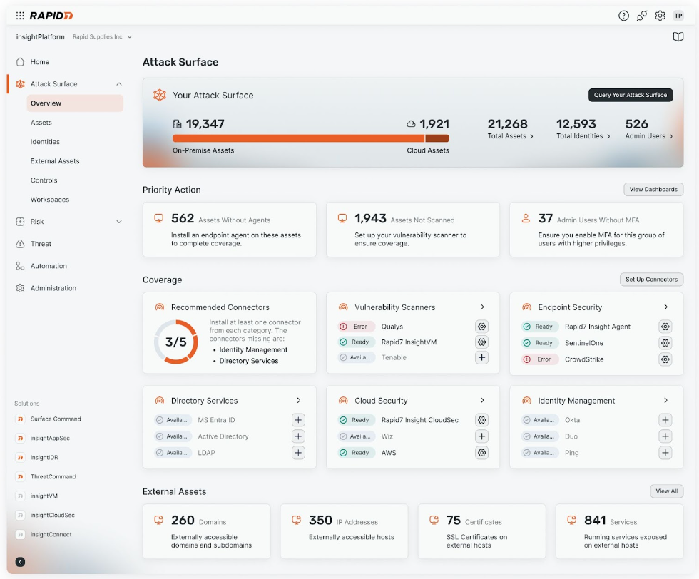
Surface Command provides the foundational attack surface visibility that underpins the Command Platform by breaking down security data silos and combining comprehensive external attack surface monitoring with internal asset visibility across hybrid environments. The result? A dynamic 360-degree view of your entire attack surface in one place. With this view, you can:
- Visualize your entire digital estate from endpoint to cloud
- Prioritize and mitigate exposures and potential threats with a risk-aware and adversary-driven view of your entire attack surface
- Identify and address misconfigurations, shadow IT, and compliance issues
Learn more about Surface Command.
Exposure Command: Pinpoint and extinguish critical risks from endpoint to cloud
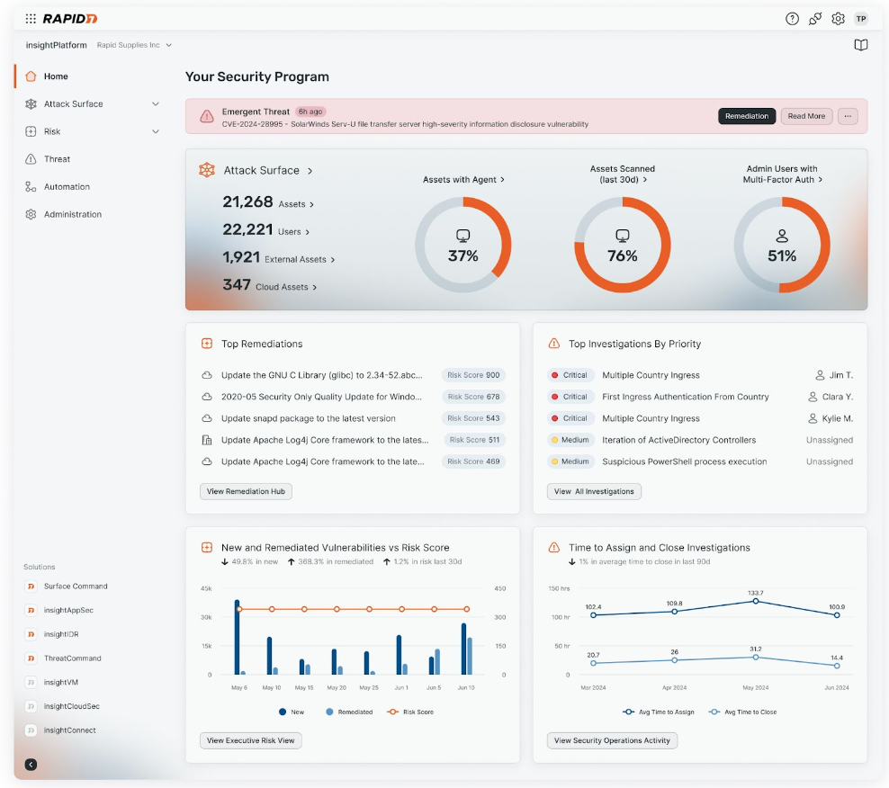
Exposure Command extends the power of Surface Command by combining complete attack surface visibility with high-fidelity risk context and insight into your organization’s security posture. Exposure Command aggregates findings from both Rapid7’s native exposure detection capabilities as well as third-party exposure and enrichment sources you’ve already got in place, so you are able to:
- Extend risk coverage to cloud environments with real-time agentless assessment
- Zero-in on exposures and vulnerabilities with the threat-aware risk context
- Continuously assess your attack surface, validate exposures, and receive actionable remediation guidance
- Efficiently operationalize your exposure management program and automate enforcement of security and compliance policies with native, no-code automation
Learn more about Exposure Command.
Continuous red teaming at your (managed) service with Vector Command
Attackers are relentlessly looking for weak spots and new access points into your organization – you should be too. Leverage Vector Command – our latest continuous red teaming service – to proactively test your external attack surface with ongoing red team exercises and expert guidance from Rapid7’s team of managed services experts.
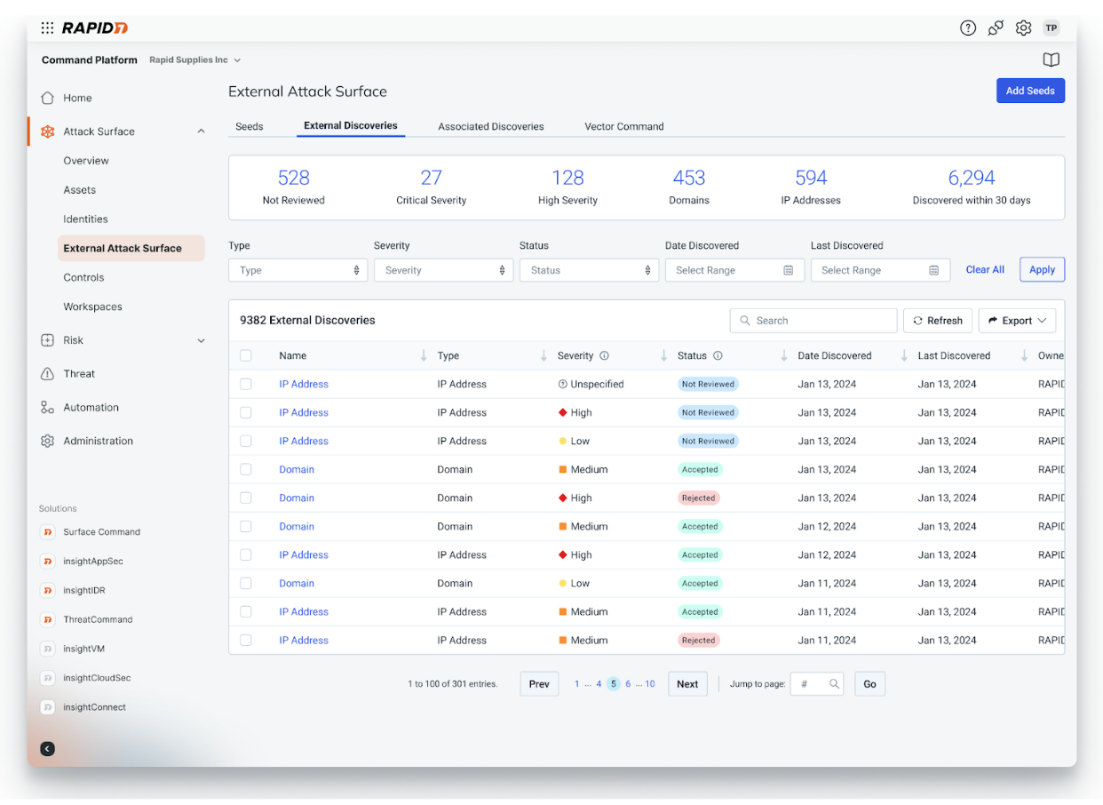
With Vector Command, your team will experience:
- Increased visibility of the external attack surface with persistent, proactive reconnaissance of both known and unknown internet-facing assets
- Improved prioritization with ongoing, expert-led red team operations to continuously validate your most critical external exposures
- Same-day reporting of successful exploits with expert-vetted attack paths for multi-vector attack chains and a curated list of “attractive assets” that are likely to be exploited
- Monthly expert consultation to confidently drive remediation efforts and resiliency planning
Learn more about Vector Command.
Improved scale, reliability and contextualized reporting for cloud and on-prem vulnerability management
The increased scale, rate of change, and complexity associated with cloud and on-prem environments makes managing vulnerabilities a challenge. This quarter we continued to advance our agentless vulnerability assessment capabilities to drive improved scalability and extended reporting to allow teams to quickly identify, prioritize, and remediate vulnerabilities at scale. This includes:
- In-cloud assessment for Azure hosts drive improved cost efficiency for running vulnerability assessments at scale across all cloud hosts running on Microsoft Azure.
- Unified cloud vulnerability reporting combines context and insights across discovered CVEs, software and resources with proof data included by default to enable more effective and accelerated vulnerability remediation.
- Increased granularity for cloud vulnerability first found dates enables teams to quickly understand where an organization is exposed to a given CVE both at an organizational level across their environment globally or on a per-resource basis.Accurately report on MTTR with first found date enhancement for on-prem vulnerabilities with the addition of “First Found” and “Reintroduced” columns, providing deeper visibility into when a vulnerability was first discovered and if it was later reintroduced after patching.
Comprehensive content coverage for policies and critical systems
We strive to provide you with fast and broad coverage for critical policies and systems so you can accurately assess the environment for vulnerability and compliance risks. This past quarter we added a number of new policy coverages and enhancements to InsightVM and Nexpose, including:
- Arista EOS coverage: Arista is a popular alternative to Cisco, and this expansion provides you with broader coverage of your boundary devices and better insights into critical assets.
- Released policy coverage for DISA STIG Windows Server 2016 and Windows Server 2019; DISA STIG for Red Hat Enterprise Linux 8 and Red Hat Enterprise Linux 9; and CIS Benchmark for Fortinet Fortigate to ensure continued compliance.
- Enhanced existing coverages for critical systems like Alpine Linux, Oracle Linux, Windows Server 2022, and Debian Linux.
Pinpoint critical signals and act confidently against threats with cloud-ready detection and response
Introducing MDR for the Extended Ecosystem
In an ever-expanding cybersecurity landscape, organizations are under more pressure than ever to keep pace with the widening attack surface. That’s why we’re so excited to bring extended support and coverage capabilities to our MDR customers with the launch of Rapid7 MDR for the Extended Ecosystem. With this addition, we’re extending our service to include triage, investigation, and response to alerts from third-party tools already in use within customer organizations.
This initial release will bring support for major EPPs such as Microsoft Defender for Endpoint, CrowdStrike Falcon, and SentinelOne, with plans to extend coverage to more third-party tools across cloud, identity, and network in the coming months.
Read this recent blog entry to learn how this extension of MDR sets Rapid7 apart and brings your team coverage, protection, and peace of mind.
Rapid7 named a Leader in IDC MarketScape: Worldwide SIEM for SMB and Enterprise
We’re excited to share we’ve been recognized as a Leader in the IDC MarketScape: Worldwide SIEM for SMB 2024 Vendor Assessment (doc #US52038824, September 2024) and the IDC MarketScape: Worldwide SIEM for Enterprise 2024 Vendor Assessment (doc #US51541324, September 2024). We’re proud that IDC highlights InsightIDR’s superior threat detection content, ease of implementation, and tangible ROI – all areas where we continually invest to provide users with a streamlined, complex-free experience.
To our customers: Thank you. Your partnership, feedback, and trust fuels our dedication to delivering the detection and response functionalities you need to take command of your attack surface and keep your organization safe. Read more about the reports here.
Intuitive log search enhancements to empower practitioners of all levels
Collecting, analyzing, and correlating logs from various sources is table stakes in identifying potential threats, detecting malicious behaviors, and responding to incidents effectively. Within InsightIDR we continue to enhance our Log Search functionality to empower you to go beyond simply correlating logs so you can feel confident securing your organization and enhancing your security posture.
Reformatted Log Search not only optimizes view and streamlines accessibility, but it reduces friction with notable enhancements:
- Pre-computed queries auto-run in less than half a second and can be leveraged from our OOTB library of queries or built custom using “groupby” or “calculate” commands.
- Automatic key suggestions are provided to analysts during query building based on the log selection to ensure faster time to investigate (as opposed to recalling and populating individually).
- Using the select clause, you can leverage new key suggestions to choose those to include in your search results. You can also customize their names and order.
The latest research and intelligence from Rapid7 Labs
Ransomware Radar Report: Findings and insights into the booming ransomware space
According to Rapid7 Labs Ransomware Radar Report, ransomware continues to evolve at a rapid pace. With the first half of 2024 seeing a +67% increase in the average number of ransomware groups actively posting to leak sites each month, it doesn’t appear that things are slowing down.
The report offers analysis and insights to help security practitioners understand and anticipate the latest developments around ransomware attacks. This research is based on data from Rapid7’s Incident Response and Rapid7 Labs teams as well as thousands of publicly reported ransomware incidents observed from January of 2023 through June of 2024.
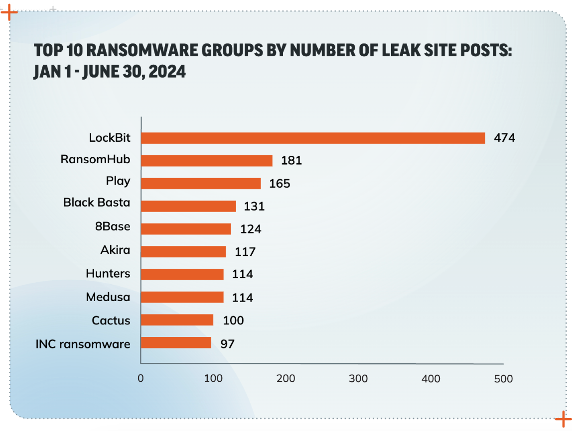
Read the Ransomware Radar Report now to learn the key takeaways for keeping your organization safe from ransomware.
Emergent Threat Response: Real-time guidance for critical threats
Rapid7’s Emergent Threat Response (ETR) program from Rapid7 Labs delivers fast, expert analysis and first-rate security content for the highest-priority security threats to help both Rapid7 customers and the greater security community understand their exposure and act quickly to defend their networks against rising threats.
In Q3, Rapid7’s Emergent Threat Response team provided expert analysis, InsightIDR and InsightVM content, and mitigation guidance for multiple critical, actively exploited vulnerabilities and widespread attacks:
- July 29: VMware ESXi CVE-2024-37085 Targeted in Ransomware Campaigns
- September 5: Rapid7 discovered and worked with the vendor to disclose CVE-2024-45195, a remote code execution vulnerability in Apache OFBiz
- September 9:
- Multiple Vulnerabilities in Veeam Backup & Replication
- CVE-2024-40766: Critical Improper Access Control Vulnerability Affecting SonicWall Devices
- September 19: High-risk vulnerabilities in common enterprise technologies, including Adobe ColdFusion CVE-2024-41874, Broadcom VMware vCenter Server CVEs (CVE-2024-38812, CVE-2024-38813), and Ivanti Endpoint Manager CVE-2024-29847
- September 26: Multiple Vulnerabilities in Common Unix Printing System (CUPS)
Follow along here to receive the latest emergent threat guidance from our team.
Stay tuned for more!
As always, we’re continuing to work on exciting product enhancements and releases throughout the year. Keep an eye on our blog and release notes as we continue to highlight the latest in product and service investments at Rapid7.
[$] An update on gccrs development
Post Syndicated from corbet original https://lwn.net/Articles/991199/
One concern that has often been expressed about the Rust language is that
there is only one compiler for it. That makes it hard to say what the
standard version of the language is and restricts the architectures that
can be targeted by Rust code to those that the available compiler supports.
Adding a Rust frontend to GCC would do much to address those concerns; at
the 2024 GNU Tools
Cauldron, Pierre-Emmanuel Patry gave an update on the state of that
work and what its objectives are.
Security updates for Tuesday
Post Syndicated from corbet original https://lwn.net/Articles/992444/
Security updates have been issued by Debian (debian-security-support, nghttp2, and sqlite3), Oracle (cups-filters, kernel, and osbuild-composer), SUSE (openssl-3), and Ubuntu (bubblewrap, flatpak and python2.7, python3.5).
Blending Zabbix and AI with Tomáš Heřmánek
Post Syndicated from Michael Kammer original https://blog.zabbix.com/blending-zabbix-and-ai-with-tomas-hermanek/28832/
Zabbix Summit 2024 is only a few days away, which means that it’s time for the last of our interviews with Summit speakers. Our final chat this year is with Tomáš Heřmánek, the CEO and Founder of initMAX s.r.o. We asked him about his beginnings in the tech industry, how he got started with Zabbix, and how AI will change the game for monitoring in general and Zabbix in particular.
Please tell us a bit about yourself and the journey that led you to initMAX.
My journey in the IT field started with small ISPs and later took a significant leap into the world of Linux and application management, where the need for effective monitoring became evident. I worked for a company that prioritized high-quality open-source solutions, and it was during this time that we adopted Zabbix version 1.8 as a replacement for Nagios, which we found to be inflexible. Shortly after our deployment, Zabbix 2.0 was released. It introduced JMX monitoring, which was crucial for us. Since then, Zabbix has been our go-to solution for monitoring.
I set a personal goal to master this outstanding monitoring system and participated in the first official Zabbix training in the Czech Republic, where I earned my initial certifications as a Zabbix Specialist and Professional on version 3.0. The training experience drew me deeper into the world of Zabbix, especially after meeting a burgeoning group of enthusiasts in the country. I felt compelled to give back to the community that had supported me.
How long have you been using Zabbix? What kind of Zabbix-related tasks does your team tackle on a daily basis?
When I started my own company, becoming a Zabbix partner was a natural choice. To further contribute to the community, I pursued the Expert and Trainer certifications. It was the most challenging 14 days of my life, but it was worth it. For anyone serious about Zabbix, I highly recommend participating in official training sessions and actively engaging with the community through forums, local groups, Telegram, WhatsApp, blogs, and forums. This commitment to support and strengthen the community further.is also why we created our own wiki, which is accessible to everyone without restrictions.
Can you give us a few clues about what we can expect to hear during your Zabbix Summit presentation?
This year, I have prepared a demonstration for the Zabbix Summit showcasing how we integrate AI into our operations, including various modifications to the web interface that allow us to automate and streamline routine tasks. Besides showcasing these innovations, we will also be making some parts of our work available to the public. The main focus of my presentation will be on problem identification, automating the creation of preprocessing steps, and using a chatbot for creating hosts, reading configurations, and making modifications. Essentially, it’s a smart assistant and guide all in one.
The final section, which we find the most challenging, deals with automated event correlation and the creation of a topology, from which correlations partially derive and evaluate. We are using the new Zabbix 7.0 feature – root cause and symptoms – for visualization in Zabbix. Our goal is to showcase not only the capabilities of Zabbix in combination with AI, but also to contribute back to the community by sharing some of these developments freely.
In your experience, does Zabbix lend itself easily to enhancement via AI?
AI is something that truly fascinates us and is currently shaping the world. From our experience, we believe that the possibilities are limited only by our imagination. In the future, I can envision AI autonomously discovering elements that need to be monitored, integrating them into Zabbix, and configuring everything necessary for effective monitoring.
What changes do you think AI will bring to the world of monitoring in general over the next decade or so?
I foresee a shift in our roles, moving away from traditional IT tasks towards a focus on idea generation, control, and the customization of artificial intelligence. As AI continues to evolve, it will not only enhance automation but also empower us to explore and implement innovative solutions more effectively.
The post Blending Zabbix and AI with Tomáš Heřmánek appeared first on Zabbix Blog.