All posts by Netflix Technology Blog

Key Challenges with Quasi Experiments at Netflix

Post Syndicated from Netflix Technology Blog original https://netflixtechblog.com/key-challenges-with-quasi-experiments-at-netflix-89b4f234b852

Kamer Toker-Yildiz, Colin McFarland, Julia Glick

At Netflix, when we can’t run A/B experiments we run quasi experiments! We run quasi experiments with various objectives such as non-member experiments focusing on acquisition, member experiments focusing on member engagement, or video streaming experiments focusing on content delivery. Consolidating on one methodology could be a challenge, as we may face different design or data constraints or optimization goals. We discuss some key challenges and approaches Netflix has been using to handle small sample size and limited pre-intervention data in quasi experiments.
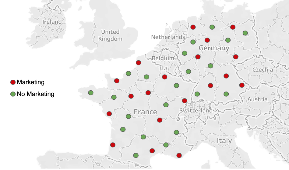
Within-country quasi design to measure the impact of TV ads in France and Germany. Geographic units are defined based on the lowest level of media buying capability.

Design and Randomization

We face various business problems where we cannot run individual level A/B tests but can benefit from quasi experiments. For instance, consider the case where we want to measure the impact of TV or billboard advertising on member engagement. It is impossible for us to have identical treatment and control groups at the member level as we cannot hold back individuals from such forms of advertising. Our solution is to randomize our member base at the smallest possible level. For instance, TV advertising can be bought at TV media market level only in most countries. This usually involves groups of cities in closer geographic proximity.

One of the major problems we face in quasi experiments is having small sample size where asymptotic properties may not practically hold. We typically have a small number of geographic units due to test limitations and also use broader or distant groups of units to minimize geographic spillovers. We are also more likely to face high variation and uneven distributions in treatment and control groups due to heterogeneity across units. For example, let’s say we are interested in measuring the impact of marketing Lost in Space series on sci-fi viewing in the UK. London with its high population is randomly assigned to the treatment cell, and people in London love sci-fi much more than other cities. If we ignore the latter fact, we will overestimate the true impact of marketing — which is now confounded. In summary, simple randomization and mean comparison we typically utilize in A/B testing with millions of members may not work well for quasi experiments.

Completely tackling these problems during the design phase may not be possible. We use some statistical approaches during design and analysis to minimize bias and maximize precision of our estimates. During design, one approach we utilize is running repeated randomizations, i.e. ‘re-randomization’. In particular, we keep randomizing until we find a randomization that gives us the maximum desired level of balance on key variables across test cells. This approach generally enables us to define more similar test groups (i.e. getting closer to apples to apples comparison). However, we may still face two issues: 1) we can only simultaneously balance on a limited number of observed variables, and it is very difficult to find identical geographic units on all dimensions, and 2) we can still face noisy results with large confidence intervals due to small sample size. We next discuss some of our analysis approaches to further tackle these problems.

Analysis

Going Beyond Simple Comparisons

Difference in differences (diff-in-diff or DID) comparison is a very common approach used in quasi experiments. In diff-in-diff, we usually consider two time periods; pre and post intervention. We utilize the pre-intervention period to generate baselines for our metrics, and normalize post intervention values by the baseline. This normalization is a simple but very powerful way of controlling for inherent differences between treatment and control groups. For example, let’s say our success metric is signups and we are running a quasi experiment in France. We have Paris and Lyon in two test cells. We cannot directly compare signups in two cities as populations are very different. Normalizing with respect to pre-intervention signups would reduce variation and help us make comparisons at the same scale. Although the diff-in-diff approach generally works reasonably well, we have observed some cases where it may not be as applicable as we discuss next.

Success Metrics With Historical Observations But Small Sample Size

In our non-member focused tests, we can observe historical acquisition metrics, e.g. signup counts, however, we don’t typically observe any other information about non-members. High variation in outcome metrics combined with small sample size can be a problem to design a well powered experiment using traditional diff-in-diff like approaches. To tackle this problem, we try to implement designs involving multiple interventions in each unit over an extended period of time whenever possible (i.e. instead of a typical experiment with single intervention period). This can help us gather enough evidence to run a well-powered experiment even with a very small sample size (i.e. few geographic units).

In particular, we turn the intervention (e.g. advertising) “on” and “off” repeatedly over time in different patterns and geographic units to capture short term effects. Every time we “toggle” the intervention, it gives us another chance to read the effect of the test. So even if we only have few geographic units, we can eventually read a reasonably precise estimate of the effect size (although, of course, results may not be generalizable to others if we have very few units). As our analysis approach, we can use observations from steady-state units to estimate what would otherwise have happened in units that are changing. To estimate the treatment effect, we fit a dynamic linear model (aka DLM), a type of state space model where the observations are conditionally Gaussian. DLMs are a very flexible category of models, but we only use a narrow subset of possible DLM structures to keep things simple. We currently have a robust internal package embedded in our internal tool, Quasimodo, to cover experiments that have similar structure. Our model is comparable to Google’s CausalImpact package, but uses a multivariate structure to let us analyze more than a single point-in-time intervention in a single region.

Success Metrics Without Historical Observations

In our member focused tests, we sometimes face cases where we don’t have success metrics with historical observations. For example, Netflix promotes its new shows that are yet to be launched on service to increase member engagement once the show is available. For a new show, we start observing metrics only when the show launches. As a result, our success metrics inherently don’t have any historical observations making it impossible to utilize the benefits of similar time series based approaches.

In these cases, we utilize the benefits of richer member data to measure and control for members’ inherent engagement or interest with the show. We do this by using relevant pre-treatment proxies, e.g. viewing of similar shows, interest in Netflix originals or similar genres. We have observed that controlling for geographic as well as individual level differences work best in minimizing confounding effects and improving precision. For example, if members in Toronto watch more Netflix originals than members in other cities in Canada, we should then control for pre-treatment Netflix originals viewing at both individual and city level to capture within and between unit variation separately.

This is in nature very similar to covariate adjustment. However, we do more than just running a simple regression with a large set of control variables. At Netflix, we have worked on developing approaches at the intersection of regression covariate adjustment and machine learning based propensity score matching by using a wide set of relevant member features. Such combined approaches help us explicitly control for members’ inherent interest in the new show using hundreds of features while minimizing linearity assumptions and degrees of freedom challenges we may face. We thus gain significant wins in both reducing potential confounding effects as well as maximizing precision to more accurately capture the treatment effect we are interested in.

Next Steps

We have excelled in the quasi experimentation space with many measurement strategies now in play across Netflix for various use cases. However we are not done yet! We can expand methodologies to more use cases and continue to improve the measurement. As an example, another exciting area we have yet to explore is combining these approaches for those metrics where we can use both time series approaches and a rich set of internal features (e.g. general member engagement metrics). If you’re interested in working on these and other causal inference problems, join our dream team!


Key Challenges with Quasi Experiments at Netflix was originally published in Netflix TechBlog on Medium, where people are continuing the conversation by highlighting and responding to this story.
Optimized shot-based encodes for 4K: Now streaming!

Post Syndicated from Netflix Technology Blog original https://netflixtechblog.com/optimized-shot-based-encodes-for-4k-now-streaming-47b516b10bbb

by Aditya Mavlankar, Liwei Guo, Anush Moorthy and Anne Aaron

Netflix has an ever-expanding collection of titles which customers can enjoy in 4K resolution with a suitable device and subscription plan. Netflix creates premium bitstreams for those titles in addition to the catalog-wide 8-bit stream profiles¹. Premium features comprise a title-dependent combination of 10-bit bit-depth, 4K resolution, high frame rate (HFR) and high dynamic range (HDR) and pave the way for an extraordinary viewing experience.

The premium bitstreams, launched several years ago, were rolled out with a fixed-bitrate ladder, with fixed 4K resolution bitrates — 8, 10, 12 and 16 Mbps — regardless of content characteristics. Since then, we’ve developed algorithms such as per-title encode optimizations and per-shot dynamic optimization, but these innovations were not back-ported on these premium bitstreams. Moreover, the encoding group of pictures (GoP) duration (or keyframe period) was constant throughout the stream causing additional inefficiency due to shot boundaries not aligning with GoP boundaries.

As the number of 4K titles in our catalog continues to grow and more devices support the premium features, we expect these video streams to have an increasing impact on our members and the network. We’ve worked hard over the last year to leapfrog to our most advanced encoding innovations — shot-optimized encoding and 4K VMAF model — and applied those to the premium bitstreams. More specifically, we’ve improved the traditional 4K and 10-bit ladder by employing

In this blog post, we present benefits of applying the above-mentioned optimizations to standard dynamic range (SDR) 10-bit and 4K streams (some titles are also HFR). As for HDR, our team is currently developing an HDR extension to VMAF, Netflix’s video quality metric, which will then be used to optimize the HDR streams.

¹ The 8-bit stream profiles go up to 1080p resolution.

Bitrate versus quality comparison

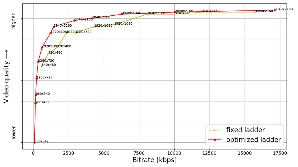
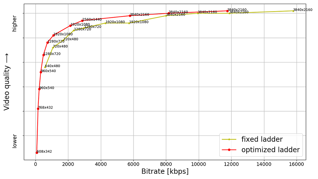
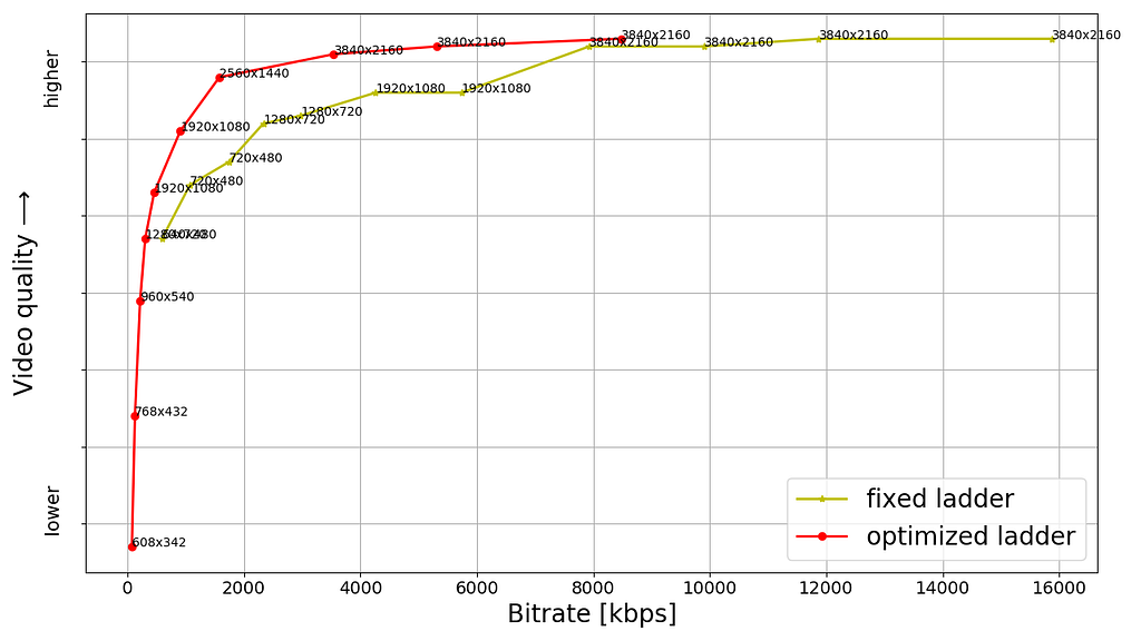
For a sample of titles from the 4K collection, the following plots show the rate-quality comparison of the fixed-bitrate ladder and the optimized ladder. The plots have been arranged in decreasing order of the new highest bitrate — which is now content adaptive and commensurate with the overall complexity of the respective title.

Fig. 1: Example of a thriller-drama episode showing new highest bitrate of 11.8 Mbps
Fig. 2: Example of a sitcom episode with some action showing new highest bitrate of 8.5 Mbps
Fig. 3: Example of a sitcom episode with less action showing new highest bitrate of 6.6 Mbps
Fig. 4: Example of a 4K animation episode showing new highest bitrate of 1.8 Mbps

The bitrate as well as quality shown for any point is the average for the corresponding stream, computed over the duration of the title. The annotation next to the point is the corresponding encoding resolution; it should be noted that video received by the client device is decoded and scaled to the device’s display resolution. As for VMAF score computation, for encoding resolutions less than 4K, we follow the VMAF best practice to upscale to 4K assuming bicubic upsampling. Aside from the encoding resolution, each point is also associated with an appropriate pixel aspect ratio (PAR) to achieve a target 16:9 display aspect ratio (DAR). For example, the 640×480 encoding resolution is paired with a 4:3 PAR to achieve 16:9 DAR, consistent with the DAR for other points on the ladder.

The last example, showing the new highest bitrate to be 1.8 Mbps, is for a 4K animation title episode which can be very efficiently encoded. It serves as an extreme example of content adaptive ladder optimization — it however should not to be interpreted as all animation titles landing on similar low bitrates.

The resolutions and bitrates for the fixed-bitrate ladder are pre-determined; minor deviation in the achieved bitrate is due to rate control in the encoder implementation not hitting the target bitrate precisely. On the other hand, each point on the optimized ladder is associated with optimal bit allocation across all shots with the goal of maximizing a video quality objective function while resulting in the corresponding average bitrate. Consequently, for the optimized encodes, the bitrate varies shot to shot depending on relative complexity and overall bit budget and in theory can reach the respective codec level maximum. Various points are constrained to different codec levels, so receivers with different decoder level capabilities can stream the corresponding subset of points up to the corresponding level.

The fixed-bitrate ladder often appears like steps — since it is not title adaptive it switches “late” to most encoding resolutions and as a result the quality stays flat within that resolution even with increasing bitrate. For example, two 1080p points with identical VMAF score or four 4K points with identical VMAF score, resulting in wasted bits and increased storage footprint.

On the other hand, the optimized ladder appears closer to a monotonically increasing curve — increasing bitrate results in an increasing VMAF score. As a side note, we do have some additional points, not shown in the plots, that are used in resolution limited scenarios — such as a streaming session limited to 720p or 1080p highest encoding resolution. Such points lie under (or to the right of) the convex hull main ladder curve but allow quality to ramp up in resolution limited scenarios.

Challenging-to-encode content

For the optimized ladders we have logic to detect quality saturation at the high end, meaning an increase in bitrate not resulting in material improvement in quality. Once such a bitrate is reached it is a good candidate for the topmost rung of the ladder. An additional limit can be imposed as a safeguard to avoid excessively high bitrates.

Sometimes we ingest a title that would need more bits at the highest end of the quality spectrum — even higher than the 16 Mbps limit of the fixed-bitrate ladder. For example,

  • a rock concert with fast-changing lighting effects and other details or
  • a wildlife documentary with fast action and/or challenging spatial details.

This scenario is generally rare. Nevertheless, below plot highlights such a case where the optimized ladder exceeds the fixed-bitrate ladder in terms of the highest bitrate, thereby achieving an improvement in the highest quality.

As expected, the quality is higher for the same bitrate, even when compared in the low or medium bitrate regions.

Fig. 5: Example of a movie with action and great amount of rich spatial details showing new highest bitrate of 17.2 Mbps

Visual examples

As an example, we compare the 1.75 Mbps encode from the fixed-bitrate ladder with the 1.45 Mbps encode from the optimized ladder for one of the titles from our 4K collection. Since 4K resolution entails a rather large number of pixels, we show 1024×512 pixel cutouts from the two encodes. The encodes are decoded and scaled to a 4K canvas prior to extracting the cutouts. We toggle between the cutouts so it is convenient to spot differences. We also show the corresponding full frame which helps to get a sense of how the cutout fits in the corresponding video frame.

Fig. 6: Pristine full frame — the purpose is to give a sense of how below cutouts fit in the frame
Fig. 7: Toggling between 1024×512 pixel cutouts from two encodes as annotated. Corresponding to pristine frame shown in Figure 6.
Fig. 8: Pristine full frame — the purpose is to give a sense of how below cutouts fit in the frame
Fig. 9: Toggling between 1024×512 pixel cutouts from two encodes as annotated. Corresponding to pristine frame shown in Figure 8.
Fig. 10: Pristine full frame — the purpose is to give a sense of how below cutouts fit in the frame
Fig. 11: Toggling between 1024×512 pixel cutouts from two encodes as annotated. Corresponding to pristine frame shown in Figure 10.
Fig. 12: Pristine full frame — the purpose is to give a sense of how below cutouts fit in the frame
Fig. 13: Toggling between 1024×512 pixel cutouts from two encodes as annotated. Corresponding to pristine frame shown in Figure 12.
Fig. 14: Pristine full frame — the purpose is to give a sense of how below cutouts fit in the frame
Fig. 15: Toggling between 1024×512 pixel cutouts from two encodes as annotated. Corresponding to pristine frame shown in Figure 14.

As can be seen, the encode from the optimized ladder delivers crisper textures and higher detail for less bits. At 1.45 Mbps it is by no means a perfect 4K rendition, but still very commendable for that bitrate. There exist higher bitrate points on the optimized ladder that deliver impeccable 4K quality, also for less bits compared to the fixed-bitrate ladder.

Compression and bitrate ladder improvements

Even before testing the new streams in the field, we observe the following advantages of the optimized ladders vs the fixed ladders, evaluated over 100 sample titles:

  • Computing the Bjøntegaard Delta (BD) rate shows 50% gains on average over the fixed-bitrate ladder. Meaning, on average we need 50% less bitrate to achieve the same quality with the optimized ladder.
  • The highest 4K bitrate on average is 8 Mbps which is also a 50% reduction compared to 16 Mbps of the fixed-bitrate ladder.
  • As mobile devices continue to improve, they adopt premium features (other than 4K resolution) like 10-bit and HFR. These video encodes can be delivered to mobile devices as well. The fixed-bitrate ladder starts at 560 kbps which may be too high for some cellular networks. The optimized ladder, on the other hand, has lower bitrate points that are viable in most cellular scenarios.
  • The optimized ladder entails a smaller storage footprint compared to the fixed-bitrate ladder.
  • The new ladder considers adding 1440p resolution (aka QHD) points if they lie on the convex hull of rate-quality tradeoff and most titles seem to get the 1440p treatment. As a result, when averaged over 100 titles, the bitrate required to jump to a resolution higher than 1080p (meaning either QHD or 4K) is 1.7 Mbps compared to 8 Mbps of the fixed-bitrate ladder. When averaged over 100 titles, the bitrate required to jump to 4K resolution is 3.2 Mbps compared to 8 Mbps of the fixed-bitrate ladder.

Benefits to members

At Netflix we perform A/B testing of encoding optimizations to detect any playback issues on client devices as well as gauge the benefits experienced by our members. One set of streaming sessions receives the default encodes and the other set of streaming sessions receives the new encodes. This in turn allows us to compare error rates as well as various metrics related to quality of experience (QoE). Although our streams are standard compliant, the A/B testing can and does sometimes find device-side implementations with minor gaps; in such cases we work with our device partners to find the best remedy.

Overall, while A/B testing these new encodes, we have seen the following benefits, which are in line with the offline evaluation covered in the previous section:

  • For members with high-bandwidth connections we deliver the same great quality at half the bitrate on average.
  • For members with constrained bandwidth we deliver higher quality at the same (or even lower) bitrate — higher VMAF at the same encoding resolution and bitrate or even higher resolutions than they could stream before. For example, members who were limited by their network to 720p can now be served 1080p or higher resolution instead.
  • Most streaming sessions start with a higher initial quality.
  • The number of rebuffers per hour go down by over 65%; members also experience fewer quality drops while streaming.
  • The reduced bitrate together with some Digital Rights Management (DRM) system improvements (not covered in this blog) result in reducing the initial play delay by about 10%.

Next steps

We have started re-encoding the 4K titles in our catalog to generate the optimized streams and we expect to complete in a couple of months. We continue to work on applying similar optimizations to our HDR streams.

Acknowledgements

We thank Lishan Zhu for help rendered during A/B testing.

This is a collective effort on the part of our larger team, known as Encoding Technologies, and various other teams that we have crucial partnerships with, such as:

If you are passionate about video compression research and would like to contribute to this field, we have an open position.


Optimized shot-based encodes for 4K: Now streaming! was originally published in Netflix TechBlog on Medium, where people are continuing the conversation by highlighting and responding to this story.