Sponsorship for the Openwall lists

Post Syndicated from corbet original https://lwn.net/Articles/950538/

Alexander “Solar Designer” Peslyak, the longtime maintainer of the
oss-security and linux-distros mailing lists, has announced
that this work has gained a sponsor:

After 15+ years of being a 100% volunteer effort, Openwall’s
maintenance of oss-security and (linux-)distros is finally
sponsored by the OpenSSF, a project of the Linux Foundation. This
sponsorship does not provide the Linux Foundation with the ability
to set policies for community resources managed by Openwall. I am
grateful for the support, which will help ensure continued
operation of these resources on a new level while retaining
independence.

As part of this arrangement, Peslyak is now producing statistics on
vulnerability handling; the first
set for 2023
has been posted.

Fedora 39 released

Post Syndicated from corbet original https://lwn.net/Articles/950524/

Fedora
39
has been released, one day after the Fedora project’s 20th
anniversary. See the list of
approved changes
and this Fedora
Magazine article
for more information.

As always, we’ve updated many, many other packages as we work to
bring you the best of everything the free and open source software
world has to offer. Fedora Linux 39 includes gcc 13.2, binutils
2.40, glibc 2.38, gdb 13.2, and rpm 4.19. It also has updates to
popular programming language stacks, including Python 3.12 and Rust
1.73.

Security updates for Tuesday

Post Syndicated from corbet original https://lwn.net/Articles/950523/

Security updates have been issued by Debian (trapperkeeper-webserver-jetty9-clojure), Mageia (libsndfile, packages, thunderbird, and x11-server), Oracle (.NET 6.0), SUSE (kernel, kubevirt, virt-api-container, virt-controller-container, virt-handler-container, virt-launcher-container, virt-libguestfs-tools- container, virt-operator-container, redis, and squid), and Ubuntu (gsl).

New micro:bit coding projects for kids

Post Syndicated from Author original https://www.raspberrypi.org/blog/microbit-coding-projects/

Young people can now learn to code and create with our brand-new path of micro:bit coding projects. The ‘Intro to micro:bit’ path is free and kids can follow it to code projects that focus on wellbeing, including topics like mental health, relaxation, and exercise.

As you might know, a micro:bit (pronounced “microbit”) is a small, programmable device designed for education. You can program it using any computer. It’s easy to use and learn with, and suitable for beginners, especially young people in and out of school.

The theme of the new project path: Wellbeing

Our aim for this new micro:bit project path is to help young people explore how they can create their own tech tools that help them look after themselves and others. By designing the micro:bit coding projects around wellbeing, we want to not only help kids develop programming and digital literacy skills, but also promote open conversations about the important topic of mental health.

Kids coding a microbit project.
Credit: David Bird

The six micro:bit coding projects in our new path all cover different aspects of wellbeing in a fun, creative way:

  1. Good sleep patterns
  2. Relaxation
  3. Self-confidence
  4. Happiness
  5. Health 
  6. Entertainment

We hope that following the path and making projects helps encourage learners to ask questions, share their experiences, and feel like they can ask parents, teachers, or mentors for support, and help support their friends and peers.

What is in the ‘Intro to micro:bit’ project path?

The ‘Intro to micro:bit’ path is designed according to our Digital Making Framework. Its aim is to encourage young people to become independent coders and tech creators as they progress along the projects in a path by gently removing scaffolding.

  • Our project paths begin with three Explore projects, in which learners are guided through tasks that introduce them to new coding skills.
  • Next, learners complete two Design projects. Here, they are encouraged to practise their skills and bring in their own interests to personalise their coding creations.
  • Finally, learners complete one Invent project. This is where they put everything that they have learned together and create something unique that matters to them.

The structure of the path means that learners are led through the development process of a coding project and learn how to turn their ideas into reality. The path structure also supports them with fixing programming errors (debugging), showing them that errors are a normal part of computer programming and just temporary setbacks that they can overcome.

Credit: David Bird

Because community is important for learning, the path also offers young people the chance to share the projects they make with peers around the world.

What coding skills and knowledge will young people learn?

The Explore projects at the start of the path are where the initial learning takes place. Learners then develop their new skills and knowledge by putting them into practice in the Design and Invent projects, where they add in their own ideas and creativity.

The key programming concepts covered in this path are:

  • Variables
  • Using selection (if, else if, and else)
  • Using repetition (for loops)
  • Using randomisation
  • Using functions
Kids coding a microbit project.
Credit: David Bird

There are two versions of the micro:bit (V1 and V2) and learners can use either version to create the micro:bit coding projects in the path, using the micro:bit’s input and output features:

Input features:

  • Buttons
  • Accelerometer
  • Sound sensor/microphone (micro:bit V2 only)
  • Capacitive touch sensor
  • Light sensor

Output features:

  • LED display
  • Speaker
  • Headphones connected via GPIO (micro:bit V1 only)

Explore project 1: Music player

In this Explore project, kids create a music player on the micro:bit to explore how listening to music can improve their mood. While creating their music player, young people get to choose melodies that they enjoy or that make them feel more relaxed. They also add a range of functions such as pausing, skipping, and shuffling tracks.

Explore project 2: Sound level meter

Noise levels can affect people’s well-being, so in this project, kids create a program to use the micro:bit to display how noisy their environment is. They will also learn how to save the noise data the micro:bit measures so they can identify the noisiest times in their day.

Explore project 3: Sleep tracker

Sleep is an important factor that contributes towards well-being. With this third Explore project, kids create a program to track their sleep movements using the micro:bit. This teaches them about variables and about using the micro:bit’s accelerometer, and its LEDs to display data.

Design project 1: How’s your day?

The first Design project of the path gets young people to build a mood checker program using the question ‘How’s your day?’. Kids get creative design control over the mood checker’s outputs according to the user’s replies, including displaying an animation or positive messages, or playing music. Kids can also make use of sensors to measure the various factors in the environment that could be affecting the user’s mood.

In this project, young people apply all of the coding skills and knowledge covered in the Explore projects, including selection, repetition, variables, functions, and randomisation.

Design project 2: Active assistant

In the second Design project, young people create an assistant that helps them get active.The project provides examples, a structure, and brief summaries of what kids have learned to do on the path so far to inspire and motivate them. This mean young people can work independently to produce their own outcomes and the functionality of their assistant is up to each young tech creator.

Invent project: Party game

The final project, Party game, encourages learners to independently replicate their favourite party game for entertainment and relaxation. Learners will combine all of the knowledge and skills they’ve gained throughout the path to make something of their own around the theme of well-being. This is a chance for them to unleash their creativity and reflect on real-life games they enjoy. The outcome will be unique, and fun for them to share with their friends and family.

Key questions answered

Who is this path for?

We have written these micro:bit coding projects with young people around the age of 6 to 13 in mind. Building the projects on the path does not require any previous coding experience, although complete beginners may want to try our free ‘Intro to Scratch’ path first.

What software do learners need to code these projects?

A web browser on a computer. In every project, starter code is provided in the MakeCode online code editor. Learners can either download their project code to a physical micro:bit (recommended) or use the micro:bit simulator in MakeCode.

Kids coding a microbit project.
Credit: David Bird

Young people who live where there isn’t constant internet connectivity can also download the offline version of the MakeCode editor. There are also free micro:bit coding apps for smartphones and tablets.

How long will the path take to complete?

We’ve designed the ‘Intro to micro:bit’ path to be completed in six one-hour sessions, with one hour per project. However, the project instructions invite learners to take additional time to upgrade their projects if they wish.

What can learners do next?

Take part in Coolest Projects

At the end of the micro:bit path, learners are encouraged to register a project they’re making with their new coding skills for Coolest Projects, our annual online technology showcase for young people around the world.

Taking part is free, and beginners as well as more experienced young tech creators are invited. This is their opportunity to share their ingenuity in an online gallery for the world and the Coolest Projects community to celebrate.

The post New micro:bit coding projects for kids appeared first on Raspberry Pi Foundation.

Introducing Amazon MWAA support for Apache Airflow version 2.7.2 and deferrable operators

Post Syndicated from Manasi Bhutada original https://aws.amazon.com/blogs/big-data/introducing-amazon-mwaa-support-for-apache-airflow-version-2-7-2-and-deferrable-operators/

Amazon Managed Workflow for Apache Airflow (Amazon MWAA) is a managed service that allows you to use a familiar Apache Airflow environment with improved scalability, availability, and security to enhance and scale your business workflows without the operational burden of managing the underlying infrastructure.

Today, we are announcing the availability of Apache Airflow version 2.7.2 environments and support for deferrable operators on Amazon MWAA. In this post, we provide an overview of deferrable operators and triggers, including a walkthrough of an example showcasing how to use them. We also delve into some of the new features and capabilities of Apache Airflow, and how you can set up or upgrade your Amazon MWAA environment to version 2.7.2.

Deferrable operators and triggers

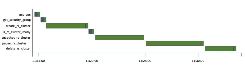
Standard operators and sensors continuously occupy an Airflow worker slot, regardless of whether they are active or idle. For example, even while waiting for an external system to complete a job, a worker slot is consumed. The Gantt chart below, representing a Directed Acyclic Graph (DAG), showcases this scenario through multiple Amazon Redshift operations.

Gantt chart representing DAG idle time

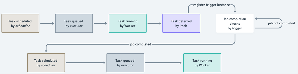
You can see the time each task spends idling while waiting for the Redshift cluster to be created, snapshotted, and paused. With the introduction of deferrable operators in Apache Airflow 2.2, the polling process can be offloaded to ensure efficient utilization of the worker slot. A deferrable operator can suspend itself and resume once the external job is complete, instead of continuously occupying a worker slot. This minimizes queued tasks and leads to a more efficient utilization of resources within your Amazon MWAA environment. The following figure shows a simplified diagram describing the process flow.

After a task has deferred its run, it frees up the worker slot and assigns the check of completion to a small piece of asynchronous code called a trigger. The trigger runs in a parent process called a triggerer, a service that runs an asyncio event loop. The triggerer has the capability to run triggers in parallel at scale, and to signal tasks to resume when a condition is met.

The Amazon provider package for Apache Airflow has added triggers for popular AWS services like AWS Glue and Amazon EMR. In Amazon MWAA environments running Apache Airflow v2.7.2, the management and operation of the triggerer service is taken care of for you. If you prefer not to use the triggerer service, you can change the configuration mwaa.triggerer_enabled. Additionally, you can define how many triggers each triggerer can run in parallel using the configuration parameter triggerer.default_capacity. This parameter defaults to values based on your Amazon MWAA environment class. Refer to the Configuration reference in the User Guide for detailed configuration values.

When to use deferrable operators

Deferrable operators are particularly useful for tasks that submit jobs to systems external to an Amazon MWAA environment, such as Amazon EMR, AWS Glue, and Amazon SageMaker, or other sensors waiting for a specific event to occur. These tasks can take minutes to hours to complete and are primarily idle operators, making them good candidates to be replaced by their deferrable versions. Some additional use cases include:

  • File system-based operations.
  • Database operations with long running queries.

Using deferrable operators in Amazon MWAA

To use deferrable operators in Amazon MWAA, ensure you’re running Apache Airflow version 2.7 or greater in your Amazon MWAA environment, and the operators or sensors in your DAGs support deferring. Operators in the Amazon provider package expose a deferrable parameter which you can set to True to run the operator in asynchronous mode. For example, you can use S3KeySensor in asynchronous mode as follows:

wait_for_source_data = S3KeySensor (
task_id="WaitForSourceData",
bucket_name="source_bucket_name",
bucket_key = "object_key",
aws_conn_id="aws_default",
deferrable=True
)

You can also utilize various pre-built deferrable operators available in other provider packages, such as Snowflake and Databricks.

Follow the complete sample code in the GitHub repository to understand how deferrable operators work together. You will be building and orchestrating the data pipeline illustrated in the following figure.

The pipeline consists of three stages:

  • A S3KeySensor that waits for a dataset to be uploaded in Amazon Simple Storage Service (Amazon S3)
  • An AWS Glue crawler to classify objects in the dataset and save schemas into the AWS Glue Data Catalog
  • An AWS Glue job that uses the metadata in the Data Catalog to denormalize the source dataset, create Data Catalog tables based on filtered data, and write the resulting data back to Amazon S3 in separate Apache Parquet files.

Setup and Teardown tasks

It’s common to build workflows that require ephemeral resources, for example an S3 bucket to temporarily store data, databases and corresponding datasets to run quality checks, or a compute cluster to train a model in a machine learning (ML) orchestration pipeline. You need to have these resources properly configured before running work tasks, and after their run, ensure they are torn down. Doing this manually is complex. It may lead to poor readability and maintainability of your DAGs, and leave resources running constantly, thereby increasing costs. With Amazon MWAA support for Apache Airflow version 2.7.2, you can use two new types of tasks to support this scenario: setup and teardown tasks.

Setup and teardown tasks ensure that the resources needed for a work task are set up before the task starts its run and then are taken down after it has finished, even if the work task fails. Any task can be configured as a setup or teardown task. Once configured, they have special visibility in the Airflow UI and also special behavior. The following graph describes a simple data quality check pipeline using setup and teardown tasks.

One option to mark setup_db_instance and teardown_db_instance as setup and teardown tasks is to use the as_teardown() method in the teardown task in the dependencies chain declaration. Note that the method receives the setup task as a parameter:

setup_db_instance >> column_quality_check >> row_count_quality_check >> teardown_db_instance.as_teardown(setups=setup_db_instance)

Another option is to use @setup and @teardown decorators:

from airflow.decorators import setup

@setup
def setup_db_instance():
...
return "Resources fully setup"

setup_db_instance()

After you configure the tasks, the graph view shows your setup tasks with an upward arrow and your teardown tasks with a downward arrow. They’re connected by a dotted line depicting the setup/teardown workflow. Any task between the setup and teardown tasks (such as column_quality_check and row_count_quality_check) are in the scope of the workflow. This arrangement involves the following behavior:

  • If you clear column_quality_check or row_count_quality_check, both setup_db_instance and teardown_db_instance will be cleared
  • If setup_db_instance runs successfully, and column_quality_check and row_count_quality_check have completed, regardless of whether they were successful or not, teardown_db_instance will run
  • If setup_db_instance fails or is skipped, then teardown_db_instance will fail or skip
  • If teardown_db_instance fails, by default Airflow ignores its status to evaluate whether the pipeline run was successful

Note that when creating setup and teardown workflows, there can be more than one set of setup and teardown tasks, and they can be parallel and nested. Neither setup nor teardown tasks are limited in number, nor are the worker tasks you can include in the scope of the workflow.

Follow the complete sample code in the GitHub repository to understand how setup and teardown tasks work.

When to use setup and teardown tasks

Setup and teardown tasks are useful to improve the reliability and cost-effectiveness of DAGs, ensuring that required resources are created and deleted in the right time. They can also help simplify complex DAGs by breaking them down into smaller, more manageable tasks, improving maintainability. Some use cases include:

  • Data processing based on ephemeral compute, like Amazon Elastic Compute Cloud (Amazon EC2) instances fleets or EMR clusters
  • ML model training or tuning pipelines
  • Extract, transform, and load (ETL) jobs using external ephemeral data stores to share data among Airflow tasks

With Amazon MWAA support for Apache Airflow version 2.7.2, you can start using setup and teardown tasks to improve your pipelines as of today. To learn more about Setup and Teardown tasks, refer to the Apache Airflow documentation.

Secrets cache

To reflect changes to your DAGs and tasks, the Apache Airflow scheduler parses your DAG files continuously, every 30 seconds by default. If you have variables or connections as top-level code (code outside the operator’s execute methods), a request is generated every time the DAG file is parsed, impacting parsing speed and leading to sub-optimal performance in the DAG file processing. If you are running at scale, it has the potential to affect Airflow performance and scalability as the amount of network communication and load on the metastore database increase. If you’re using an alternative secrets backend, such as AWS Secrets Manager, every DAG parse is a new request to that service, increasing costs.

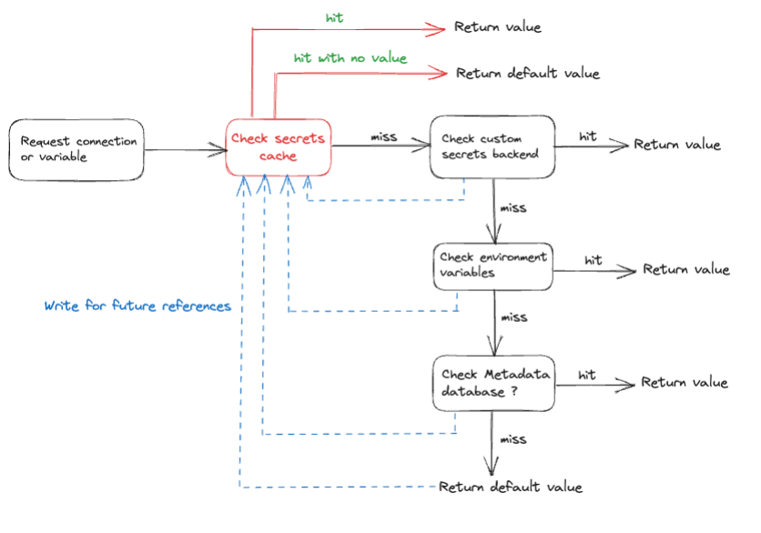
With Amazon MWAA support for Apache Airflow version 2.7.2, you can use secrets cache for variables and connections. Airflow will cache variables and connections locally so that they can be accessed faster during DAG parsing, without having to fetch them from the secrets backend, environments variables, or metadata database. The following diagram describes the process.

Enabling caching will help lower the DAG parsing time, especially if variables and connections are used in top-level code (which is not a best practice). With the introduction of a secrets cache, the frequency of API calls to the backend is reduced, which in turn lowers the overall cost associated with backend access. However, similar to other caching implementations, a secrets cache may serve outdated values until the time to live (TTL) expires.

When to use the secrets cache feature

You should consider using the secrets cache feature to improve performance and reliability, and to reduce the operating costs of your Airflow tasks. This is particularly useful if your DAG frequently retrieves variables or connections in the top-level Python code.

How to use the secrets cache feature on Amazon MWAA

To enable the secrets cache, you can set the secrets.use_cache environment configuration parameter to True. Once enabled, Airflow will automatically cache secrets when they are accessed. The cache will only be used during DAG files parsing, and not during DAG runtime.

You can also control the TTL of stored values for which the cache is considered valid using the environment configuration parameter secrets.cache_ttl_seconds, which is defaulted to 15 minutes.

Running or failed filters and Cluster Activity page

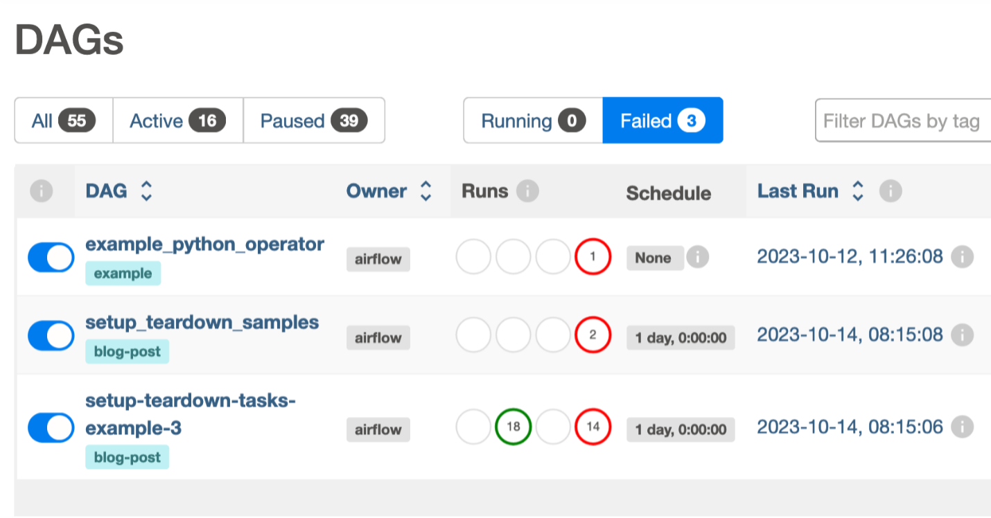
Identifying DAGs in failed state can be challenging for large Airflow instances. You typically find yourself scrolling through pages searching for failures to address. With Apache Airflow version 2.7.2 environments in Amazon MWAA, you can now filter DAGs currently running and DAGs with failed DAG runs. As you can see in the following screenshot, two status tabs, Running and Failed, were added to the UI.

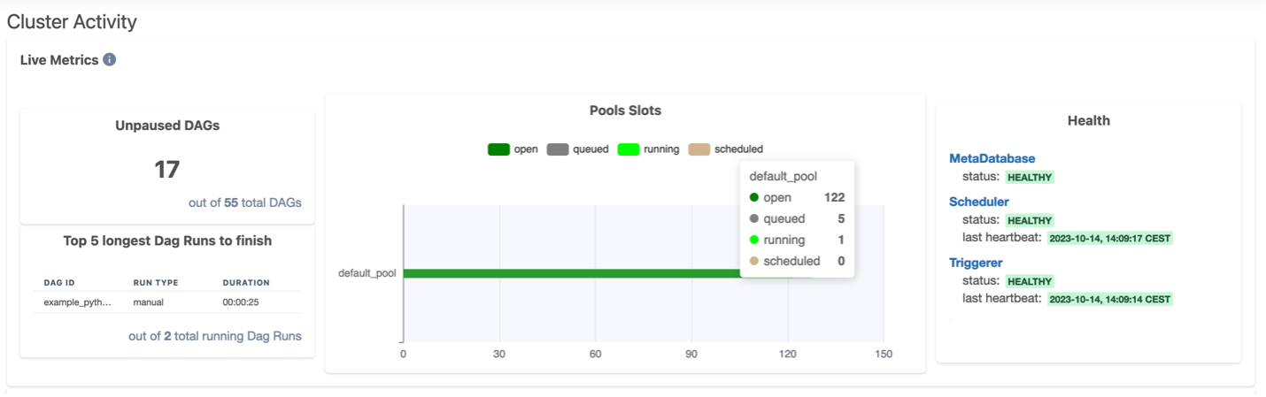
Another advantage of Amazon MWAA environments using Apache Airflow version 2.7.2 is the new Cluster Activity page for environment-level monitoring.

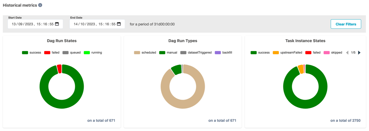
The Cluster Activity page gathers useful data to monitor your cluster’s live and historical metrics. In the top section of the page, you get live metrics on the number of DAGs ready to be scheduled, the top 5 longest running DAGs, slots used in different pools, and components health (meta database, scheduler, and triggerer). The following screenshot shows an example of this page.

The bottom section of the Cluster Activity page includes historical metrics of DAG runs and task instances states.

Set up a new Apache Airflow v2.7.2 environment in Amazon MWAA

Setting up a new Apache Airflow version 2.7.2 environment in Amazon MWAA not only provides new features, but also leverages Python 3.11 and the Amazon Linux 2023 (AL2023) base image, offering enhanced security, modern tooling, and support for the latest Python libraries and features. You can initiate the set up in your account and preferred Region using the AWS Management Console, API, or AWS Command Line Interface (AWS CLI). If you’re adopting infrastructure as code (IaC), you can automate the setup using AWS CloudFormation, the AWS Cloud Development Kit (AWS CDK), or Terraform scripts.

Upon successful creation of an Apache Airflow version 2.7.2 environment in Amazon MWAA, certain packages are automatically installed on the scheduler and worker nodes. For a complete list of installed packages and their versions, refer to this MWAA documentation. You can install additional packages using a requirements file. Beginning with Apache Airflow version 2.7.2, your requirements file must include a --constraints statement. If you do not provide a constraint, Amazon MWAA will specify one for you to ensure the packages listed in your requirements are compatible with the version of Apache Airflow you are using.

Upgrade from older versions of Apache Airflow to Apache Airflow v2.7.2

Take advantage of these latest capabilities by upgrading your older Apache Airflow v2.x-based environments to version 2.7.2 using in-place version upgrades. To learn more about in-place version upgrades, refer to Upgrading the Apache Airflow version or Introducing in-place version upgrades with Amazon MWAA.

Conclusion

In this post, we discussed deferrable operators along with some significant changes introduced in Apache Airflow version 2.7.2, such as the Cluster Activity page in the UI, the cache for variables and connections, and how you can get started using them in Amazon MWAA.

For additional details and code examples on Amazon MWAA, visit the Amazon MWAA User Guide and the Amazon MWAA examples GitHub repo.

Apache, Apache Airflow, and Airflow are either registered trademarks or trademarks of the Apache Software Foundation in the United States and/or other countries.


About the Authors

Manasi Bhutada is an ISV Solutions Architect based in the Netherlands. She helps customers design and implement well architected solutions in AWS that address their business problems. She is passionate about data analytics and networking. Beyond work she enjoys experimenting with food, playing pickleball, and diving into fun board games.

Hernan Garcia is a Senior Solutions Architect at AWS based in the Netherlands. He works in the Financial Services Industry supporting enterprises in their cloud adoption. He is passionate about serverless technologies, security, and compliance. He enjoys spending time with family and friends, and trying out new dishes from different cuisines.

Introducing faster polling scale-up for AWS Lambda functions configured with Amazon SQS

Post Syndicated from James Beswick original https://aws.amazon.com/blogs/compute/introducing-faster-polling-scale-up-for-aws-lambda-functions-configured-with-amazon-sqs/

This post was written by Anton Aleksandrov, Principal Solutions Architect, and Tarun Rai Madan, Senior Product Manager.

Today, AWS is announcing that AWS Lambda supports up to five times faster polling scale-up rate for spiky Lambda workloads configured with Amazon Simple Queue Service (Amazon SQS) as an event source.

This feature enables customers building event-driven applications using Lambda and SQS to achieve more responsive scaling during a sudden burst of messages in their SQS queues, and reduces the need to duplicate Lambda functions or SQS queues to achieve faster message processing.

Overview

Customers building modern event-driven and messaging applications with AWS Lambda use the Amazon SQS as a fundamental building block for creating decoupled architectures. Amazon SQS is a fully managed message queueing service for microservices, distributed systems, and serverless applications. When a Lambda function subscribes to an SQS queue as an event source, Lambda polls the queue, retrieves the messages, and sends retrieved messages in batches to the function handler for processing. To consume messages efficiently, Lambda detects the increase in queue depth, and increases the number of poller processes to process the queued messages.

Up until today, the Lambda was adding up to 60 concurrent executions per minute for Lambda functions subscribed to SQS queues, scaling up to a maximum of 1,250 concurrent executions in approximately 20 minutes. However, customers tell us that some of the modern event-driven applications they build using Lambda and SQS are sensitive to sudden spikes in messages, which may cause noticeable delay in processing of messages for end users. In order to harness the power of Lambda for applications that experience a burst of messages in SQS queues, these customers needed Lambda message polling to scale up faster.

With today’s announcement, Lambda functions that subscribe to an SQS queue can scale up to five times faster for queues that see a spike in message backlog, adding up to 300 concurrent executions per minute, and scaling up to a maximum of 1,250 concurrent executions. This scaling improvement helps to use the simplicity of Lambda and SQS integration to build event-driven applications that scale faster during a surge of incoming messages, particularly for real-time systems. It also offers customers the benefit of faster processing during spikes of messages in SQS queues, while continuing to offer the flexibility to limit the maximum concurrent Lambda invocations per SQS event source.

Controlling the maximum concurrent Lambda invocations by SQS

The new improved scaling rates are automatically applied to all AWS accounts using Lambda and SQS as an event source. There is no explicit action that you must take, and there’s no additional cost. This scaling improvement helps customers to build more performant Lambda applications where they need faster SQS polling scale-up. To prevent potentially overloading the downstream dependencies, Lambda provides customers the control to set the maximum number of concurrent executions at a function level with reserved concurrency, and event source level with maximum concurrency.

The following diagram illustrates settings that you can use to control the flow rate of an SQS event-source. You use reserved concurrency to control function-level scaling, and maximum concurrency to control event source scaling.

Control the flow rate of an SQS event-source

Reserved concurrency is the maximum concurrency that you want to allocate to a function. When a function has reserved concurrency allocated, no other functions can use that concurrency.

AWS recommends using reserved concurrency when you want to ensure a function has enough concurrency to scale up. When an SQS event source is attempting to scale up concurrent Lambda invocations, but the function has already reached the threshold defined by the reserved concurrency, the Lambda service throttles further function invocations.

This may result in SQS event source attempting to scale down, reducing the number of concurrently processed messages. Depending on the queue configuration, the throttled messages are returned to the queue for retrying, expire based on the retention policy, or sent to a dead-letter queue (DLQ) or on-failure destination.

The maximum concurrency setting allows you to control concurrency at the event source level. It allows you to define the maximum number of concurrent invocations the event source attempts to send to the Lambda function. For scenarios where a single function has multiple SQS event sources configured, you can define maximum concurrency for each event source separately, providing more granular control. When trying to add rate control to SQS event sources, AWS recommends you start evaluating maximum concurrency control first, as it provides greater flexibility.

Reserved concurrency and maximum concurrency are complementary capabilities, and can be used together. Maximum concurrency can help to prevent overwhelming downstream systems and throttled invocations. Reserved concurrency helps to ensure available concurrency for the function.

Example scenario

Consider your business must process large volumes of documents from storage. Once every few hours, your business partners upload large volumes of documents to S3 buckets in your account.

For resiliency, you’ve designed your application to send a message to an SQS queue for each of the uploaded documents, so you can efficiently process them without accidentally skipping any. The documents are processed using a Lambda function, which takes around two seconds to process a single document.

Processing these documents is a CPU-intensive operation, so you decide to process a single document per invocation. You want to use the power of Lambda to fan out the parallel processing to as many concurrent execution environments as possible. You want the Lambda function to scale up rapidly to process those documents in parallel as fast as possible, and scale-down to zero once all documents are processed to save costs.

When a business partner uploads 200,000 documents, 200,000 messages are sent to the SQS queue. The Lambda function is configured with an SQS event source, and it starts consuming the messages from the queue.

This diagram shows the results of running the test scenario before the SQS event source scaling improvements. As expected, you can see that concurrent executions grow by 60 per minute. It takes approximately 16 minutes to scale up to 900 concurrent executions gradually and process all the messages in the queue.

Results of running the test scenario before the SQS event source scaling improvements

The following diagram shows the results of running the same test scenario after the SQS event source scaling improvements. The timeframe used for both charts is the same, but the performance on the second chart is better. Concurrent executions grow by 300 per minute. It only takes 4 minutes to scale up to 1,250 concurrent executions, and all the messages in the queue are processed in approximately 8 minutes.

The results of running the same test scenario after the SQS event source scaling improvements

Deploying this example

Use the example project to replicate this performance test in your own AWS account. Follow the instructions in README.md for provisioning the sample project in your AWS accounts using the AWS Cloud Development Kit (CDK).

This example project is configured to demonstrate a large-scale workload processing 200,000 messages. Running this sample project in your account may incur charges. See AWS Lambda pricing and Amazon SQS pricing.

Once deployed, use the application under the “sqs-cannon” directory to send 200,000 messages to the SQS queue (or reconfigure to any other number). It takes several minutes to populate the SQS queue with messages. After all messages are sent, enable the SQS event source, as described in the README.md, and monitor the charts in the provisioned CloudWatch dashboard.

The default concurrency quota for new AWS accounts is 1000. If you haven’t requested an increase in this quota, the number of concurrent executions is capped at this number. Use Service Quotas or contact your account team to request a concurrency increase.

Security best practices

Always use the least privileged permissions when granting your Lambda functions access to SQS queues. This reduces potential attack surface by ensuring that only specific functions have permissions to perform specific actions on specific queues. For example, in case your function only polls from the queue, grant it permission to read messages, but not to send new messages. A function execution role defines which actions your function is allowed to perform on other resources. A queue access policy defines the principals that can access this queue, and the actions that are allowed.

Use server-side encryption (SSE) to store sensitive data in encrypted SQS queues. With SSE, your messages are always stored in encrypted form, and SQS only decrypts them for sending to an authorized consumer. SSE protects the contents of messages in queues using SQS-managed encryption keys (SSE-SQS) or keys managed in the AWS Key Management Service (SSE-KMS).

Conclusion

The improved Lambda SQS event source polling scale-up capability enables up to five times faster scale-up performance for spiky event-driven workloads using SQS queues, at no additional cost. This improvement offers customers the benefit of faster processing during spikes of messages in SQS queues, while continuing to offer the flexibility to limit the maximum concurrent invokes by SQS as an event source.

For more serverless learning resources, visit Serverless Land.

How to improve your security incident response processes with Jupyter notebooks

Post Syndicated from Tim Manik original https://aws.amazon.com/blogs/security/how-to-improve-your-security-incident-response-processes-with-jupyter-notebooks/

Customers face a number of challenges to quickly and effectively respond to a security event. To start, it can be difficult to standardize how to respond to a partic­ular security event, such as an Amazon GuardDuty finding. Additionally, silos can form with reliance on one security analyst who is designated to perform certain tasks, such as investigate all GuardDuty findings. Jupyter notebooks can help you address these challenges by simplifying both standardization and collaboration.

Jupyter Notebook is an open-source, web-based application to run and document code. Although Jupyter notebooks are most frequently used for data science and machine learning, you can also use them to more efficiently and effectively investigate and respond to security events.

In this blog post, we will show you how to use Jupyter Notebook to investigate a security event. With this solution, you can automate the tasks of gathering data, presenting the data, and providing procedures and next steps for the findings.

Benefits of using Jupyter notebooks for security incident response

The following are some ways that you can use Jupyter notebooks for security incident response:

  • Develop readable code for analysts – Within a notebook, you can combine markdown text and code cells to improve readability. Analysts can read context around the code cell, run the code cell, and analyze the results within the notebook.
  • Standardize analysis and response – You can reuse notebooks after the initial creation. This makes it simpler for you to standardize your incident response processes for how to respond to a certain type of security event. Additionally, you can use notebooks to achieve repeatable responses. You can rerun an entire notebook or a specific cell.
  • Collaborate and share incident response knowledge – After you create a Jupyter notebook, you can share it with peers to more seamlessly collaborate and share knowledge, which helps reduce silos and reliance on certain analysts.
  • Iterate on your incident response playbooks – Developing a security incident response program involves continuous iteration. With Jupyter notebooks, you can start small and iterate on what you have developed. You can keep Jupyter notebooks under source code control by using services such as AWS CodeCommit. This allows you to approve and track changes to your notebooks.

Architecture overview

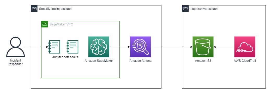
Figure 1: Architecture for incident response analysis

Figure 1: Architecture for incident response analysis

The architecture shown in Figure 1 consists of the foundational services required to analyze and contain security incidents on AWS. You create and access the playbooks through the Jupyter console that is hosted on Amazon SageMaker. Within the playbooks, you run several Amazon Athena queries against AWS CloudTrail logs hosted in Amazon Simple Storage Service (Amazon S3).

Solution implementation

To deploy the solution, you will complete the following steps:

  1. Deploy a SageMaker notebook instance
  2. Create an Athena table for your CloudTrail trail
  3. Grant AWS Lake Formation access
  4. Access the Credential Compromise playbooks by using JupyterLab

Step 1: Deploy a SageMaker notebook instance

You will host your Jupyter notebooks on a SageMaker notebook instance. We chose to use SageMaker instead of running the notebooks locally because SageMaker provides flexible compute, seamless integration with CodeCommit and GitHub, temporary credentials through AWS Identity and Access Management (IAM) roles, and lower latency for Athena queries.

You can deploy the SageMaker notebook instance by using the AWS CloudFormation template from our jupyter-notebook-for-incident-response GitHub repository. We recommend that you deploy SageMaker in your security tooling account or an equivalent.

The CloudFormation template deploys the following resources:

  • A SageMaker notebook instance to run the analysis notebooks. Because this is a proof of concept (POC), the deployed SageMaker instance is the smallest instance type available. However, within an enterprise environment, you will likely need a larger instance type.
  • An AWS Key Management Service (AWS KMS) key to encrypt the SageMaker notebook instance and protect sensitive data.
  • An IAM role that grants the SageMaker notebook permissions to query CloudTrail, VPC Flow Logs, and other log sources.
  • An IAM role that allows access to the pre-signed URL of the SageMaker notebook from only an allowlisted IP range.
  • A VPC configured for SageMaker with an internet gateway, NAT gateway, and VPC endpoints to access required AWS services securely. The internet gateway and NAT gateway provide internet access to install external packages.
  • An S3 bucket to store results for your Athena log queries—you will reference the S3 bucket in the next step.

Step 2: Create an Athena table for your CloudTrail trail

The solution uses Athena to query CloudTrail logs, so you need to create an Athena table for CloudTrail.

There are two main ways to create an Athena table for CloudTrail:

For either of these methods to create an Athena table, you need to provide the URI of an S3 bucket. For this blog post, use the URI of the S3 bucket that the CloudFormation template created in Step 1. To find the URI of the S3 bucket, see the Output section of the CloudFormation stack.

Step 3: Grant AWS Lake Formation access

If you don’t use AWS Lake Formation in your AWS environment, skip to Step 4. Otherwise, continue with the following instructions. Lake Formation is how data access control for your Athena tables is managed.

To grant permission to the Security Log database

  1. Open the Lake Formation console.
  2. Select the database that you created in Step 2 for your security logs. If you used the Security Analytics Bootstrap, then the table name is either security_analysis or a custom name that you provided—you can find the name in the CloudFormation stack. If you created the Athena table by using the CloudTrail console, then the database is named default.
  3. From the Actions dropdown, select Grant.
  4. In Grant data permissions, select IAM users and roles.
  5. Find the IAM role used by the SageMaker Notebook instance.
  6. In Database permissions, select Describe and then Grant.

To grant permission to the Security Log CloudTrail table

  1. Open the Lake Formation console.
  2. Select the database that you created in Step 2.
  3. Choose View Tables.
  4. Select CloudTrail. If you created VPC flow log and DNS log tables, select those, too.
  5. From the Actions dropdown, select Grant.
  6. In Grant data permissions, select IAM users and roles.
  7. Find the IAM role used by the SageMaker notebook instance.
  8. In Table permissions, select Describe and then Grant.

Step 4: Access the Credential Compromise playbooks by using JupyterLab

The CloudFormation template clones the jupyter-notebook-for-incident-response GitHub repo into your Jupyter workspace.

You can access JupyterLab hosted on your SageMaker notebook instance by following the steps in the Access Notebook Instances documentation.

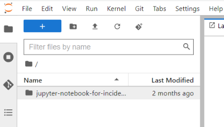
Your folder structure should match that shown in Figure 2. The parent folder should be jupyter-notebook-for-incident-response, and the child folders should be playbooks and cfn-templates.

Figure 2: Folder structure after GitHub repo is cloned to the environment

Figure 2: Folder structure after GitHub repo is cloned to the environment

Sample investigation of a spike in failed login attempts

In the following sections, you will use the Jupyter notebook that we created to investigate a scenario where failed login attempts have spiked. We designed this notebook to guide you through the process of gathering more information about the spike.

We discuss the important components of these notebooks so that you can use the framework to create your own playbooks. We encourage you to build on top of the playbook, and add additional queries and steps in the playbook to customize it for your organization’s specific business and security goals.

For this blog post, we will focus primarily on the analysis phase of incident response and walk you through how you can use Jupyter notebooks to help with this phase.

Before you get started with the following steps, open the credential-compromise-analysis.ipynb notebook in your JupyterLab environment.

How to import Python libraries and set environment variables

The notebooks require that you have the following Python libraries:

  • Boto3 – to interact with AWS services through API calls
  • Pandas – to visualize the data
  • PyAthena – to simplify the code to connect to Athena

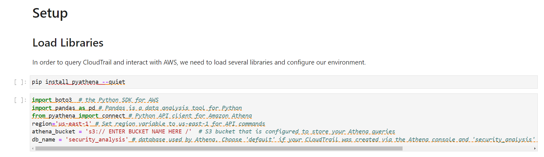
To install the required Python libraries, in the Setup section of the notebook, under Load libraries, edit the variables in the two code cells as follows:

  • region – specify the AWS Region that you want your AWS API commands to run in (for example, us-east-1).
  • athena_bucket – specify the S3 bucket URI that is configured to store your Athena queries. You can find this information at Athena > Query Editor > Settings > Query result location.
  • db_name – specify the database used by Athena that contains your Athena table for CloudTrail.
Figure 3: Load the Python libraries in the notebook

Figure 3: Load the Python libraries in the notebook

This helps ensure that subsequent code cells that run are configured to run in your environment.

Run each code cell by choosing the cell and pressing SHIFT+ENTER or by choosing the play button (▶) in the toolbar at the top of the console.

How to set up the helper function for Athena

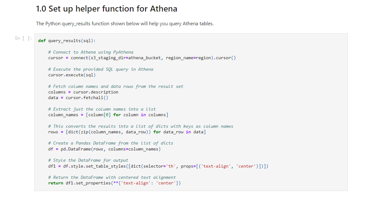
The Python query_results function, shown in the following figure, helps you query Athena tables. Run this code cell. You will use the query_results function later in the 2.0 IAM Investigation section of the notebook.

Figure 4: Code cell for the helper function to query with Athena

Figure 4: Code cell for the helper function to query with Athena

Credential Compromise Analysis Notebook

The credential-compromise-analysis.ipynb notebook includes several prebuilt queries to help you start your investigation of a potentially compromised credential. In this post, we discuss three of these queries:

  • The first query provides a broad view by retrieving the CloudTrail events related to authorization failures. By reviewing these results, you get baseline information about where users and roles are attempting to access resources or take actions without having the proper permissions.
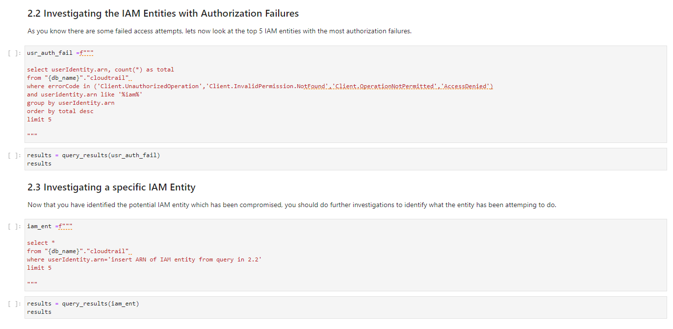
  • The second query narrows the focus by identifying the top five IAM entities (such as users, roles, and identities) that are causing most of the authorization failures. Frequent failures from specific entities often indicate that their credentials are compromised.
  • The third query zooms in on one of the suspicious entities from the previous query. It retrieves API activity and events initiated by that entity across AWS services or resource. Analyzing actions performed by a suspicious entity can reveal if valid permissions are being misused or if the entity is systematically trying to access resources it doesn’t have access to.

Investigate authorization failures

The notebook has markdown cells that provide a description of the expected result of the query. The next cell contains the query statement. The final cell calls the query_result function to run your query by using Athena and display your results in tabular format.

In query 2.1, you query for specific error codes such as AccessDenied, and filter for anything that is an IAM entity by looking for useridentity.arn like ‘%iam%’. The notebook orders the entries by eventTime. If you want to look for specific IAM Identity Center entities, update the query to filter by useridentity.sessioncontext.sessionissuer.arn like ‘%sso.amazonaws.com%’.

This query retrieves a list of failed API calls to AWS services. From this list, you can gain additional insight into the context surrounding the spike in failed login attempts.

When you investigate denied API access requests, carefully examine details such as the user identity, timestamp, source IP address, and other metadata. This information helps you determine if the event is a legitimate threat or a false positive. Here are some specific questions to ask:

  • Does the IP address originate from within your network, or is it external? Internal addresses might be less concerning.
  • Is the access attempt occurring during normal working hours for that user? Requests outside of normal times might warrant more scrutiny.
  • What resources or changes is the user trying to access or make? Attempts to modify sensitive data or systems might indicate malicious intent.

By thoroughly evaluating the context around denied API calls, you can more accurately assess the risk they pose and whether you need to take further action. You can use the specifics in the logs to go beyond just the fact that access was denied, and learn the story of who, when, and why.

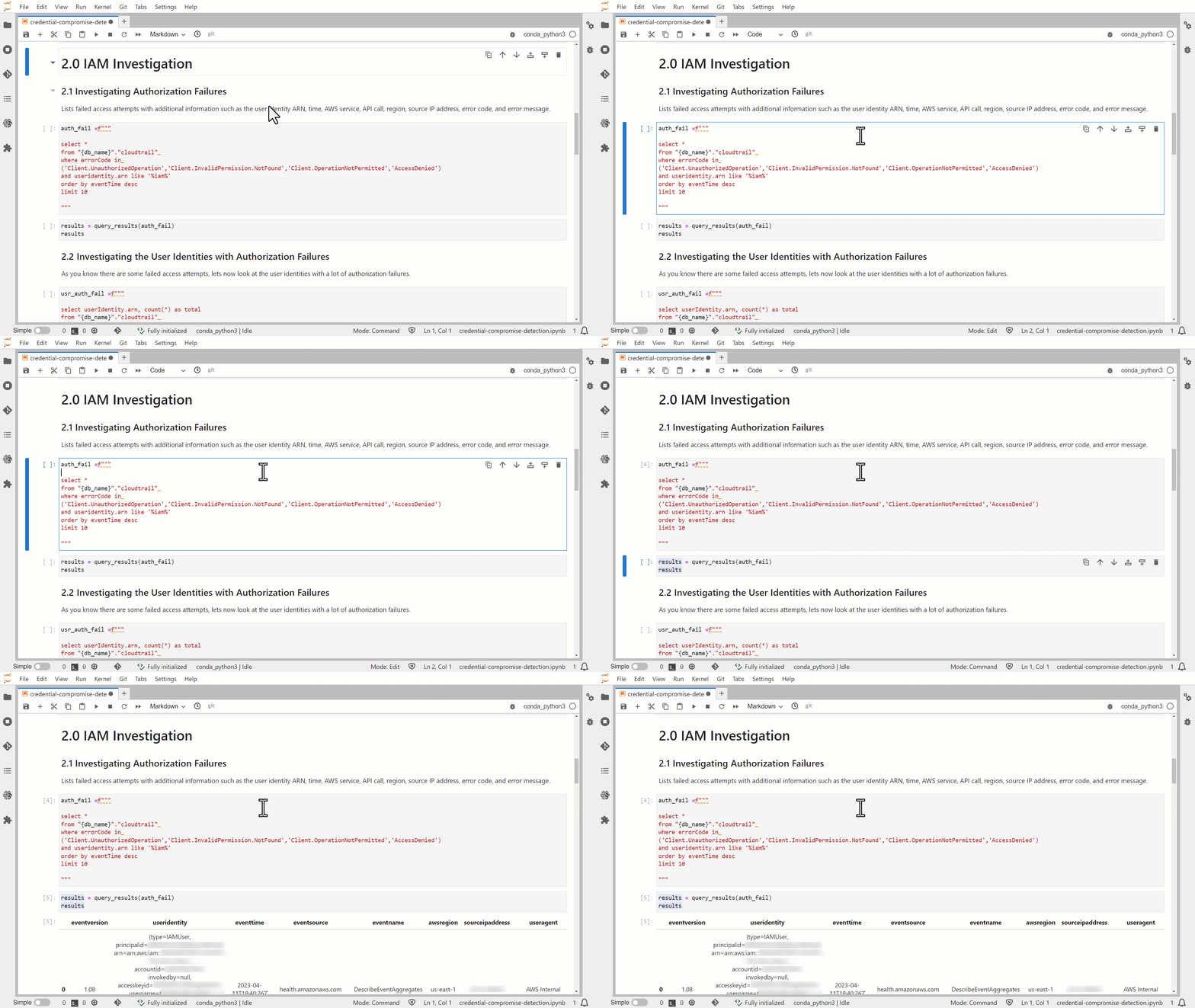
As shown in the following figure, the queries in the notebook use the following structure.

  1. Markdown cell to explain the purpose of the query (the query statement).
  2. Code cell to run the query and display the query results.

In the figure, the first code cell that runs stores the input for the query statement. After that finishes, the next code block displays the query results.

Figure 5: Run predefined Athena queries in JupyterLab

Figure 5: Run predefined Athena queries in JupyterLab

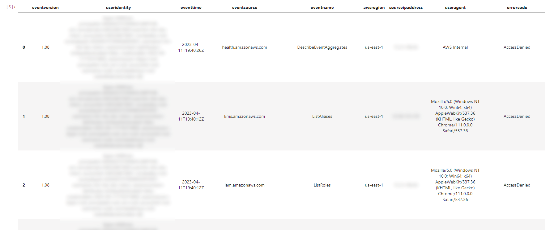
Figure 6 shows the output of the query that you ran in the 2.1 Investigation Authorization Failures section. It contains critical details for understanding the context around a denied API call:

  • The eventtime field shows the date and time that the request was completed.
  • The useridentity field reveals which IAM identity made a request.
  • The sourceipddress provides the IP address that the request was made from.
  • The useragent shows which client or app was used to make the call.
Figure 6: Results from the first investigative query

Figure 6: Results from the first investigative query

Figure 6 only shows a subset of the many details captured in CloudTrail logs. By scrolling to the right in the query output, you can view additional attributes that provide further context around the event. The CloudTrail record contents guide contains a comprehensive list of the fields included in the logs, along with descriptions of each attribute.

Often, you will need to search for more information to determine if remediation is necessary. For this reason, we have included additional queries to help you further examine the sequence of events leading up to the failed login attempt spike and after the spike occurred.

Triaging suspicious entities (Queries 2.2 and 2.3)

By running the second and third queries you can dig deeper into anomalous authorization failures. As shown in Figure 7, Query 2.2 provides the top five IAM entities with the most frequent access denials. This highlights the specific users, roles, and identities causing the most failures, which indicates potentially compromised credentials.

Query 2.3 takes the investigation further by isolating the activity from one suspicious entity. Retrieving the actions attempted by a single problematic user or role reveals useful context to determine if you need to revoke credentials. For example, is the entity probing resources that it shouldn’t have access to? Are there unusual API calls outside of normal hours? By scrutinizing an entity’s full history, you can make an informed decision on remediation.

Figure 7: Overview of queries 2.2 and 2.3

Figure 7: Overview of queries 2.2 and 2.3

You can use these two queries together to triage authorization failures: query 2 identifies high-risk entities, and query 3 gathers intelligence to drive your response. This progression from a macro view to a micro view is crucial for transforming signals into action.

Although log analysis relies on automation and queries to facilitate insights, human judgment is essential to interpret these signals and determine the appropriate response. You should discuss flagged events with stakeholders and resource owners to benefit from their domain expertise. You can export the results of your analysis by exporting your Jupyter notebook.

By collaborating with other people, you can gather contextual clues that might not be captured in the raw data. For example, an owner might confirm that a suspicious login time is expected for users in a certain time zone. By pairing automated detection with human perspectives, you can accurately assess risk and decide if credential revocation or other remediation is truly warranted. Uptime or downtime technical issues alone can’t dictate if remediation is necessary—the human element provides pivotal context.

Build your own queries

In addition to the existing queries, you can run your own queries and include them in your copy of the Credential-compromise-analysis.ipynb notebook. The AWS Security Analytics Bootstrap contains a library of common Athena queries for CloudTrail. We recommend that you review these queries before you start to build your own queries. The key takeaway is that these notebooks are highly customizable. You can use the Jupyter Notebook application to help meet the specific incident response requirements of your organization.

Contain compromised IAM entities

If the investigation reveals that a compromised IAM entity requires containment, follow these steps to revoke access:

  • For federated users, revoke their active AWS sessions according to the guidance in How to revoke federated users’ active AWS sessions. This uses IAM policies and AWS Organizations service control policies (SCPs) to revoke access to assumed roles.
  • Avoid using long-lived IAM credentials such as access keys. Instead, use temporary credentials through IAM roles. However, if you detect a compromised access key, immediately rotate or deactivate it by following the guidance in What to Do If You Inadvertently Expose an AWS Access Key. Review the permissions granted to the compromised IAM entity and consider if these permissions should be reduced after access is restored. Overly permissive policies might have enabled broader access for the threat actor.

Going forward, implement least privilege access and monitor authorization activity to detect suspicious behavior. By quickly containing compromised entities and proactively improving IAM hygiene, you can minimize the adversaries’ access duration and prevent further unauthorized access.

Additional considerations

In addition to querying CloudTrail, you can use Athena to query other logs, such as VPC Flow Logs and Amazon Route 53 DNS logs. You can also use Amazon Security Lake, which is generally available, to automatically centralize security data from AWS environments, SaaS providers, on-premises environments, and cloud sources into a purpose-built data lake stored in your account. To better understand which logs to collect and analyze as part of your incident response process, see Logging strategies for security incident response.

We recommended that you understand the playbook implementation described in this blog post before you expand the scope of your incident response solution. The running of queries and automation of containment are two elements to consider as you think about the next steps to evolve your incident response processes.

Conclusion

In this blog post, we showed how you can use Jupyter notebooks to simplify and standardize your incident response processes. You reviewed how to respond to a potential credential compromise incident using a Jupyter notebook style playbook. You also saw how this helps reduce the time to resolution and standardize the analysis and response. Finally, we presented several artifacts and recommendations showing how you can tailor this solution to meet your organization’s specific security needs. You can use this framework to evolve your incident response process.

Further resources

If you have feedback about this post, submit comments in the Comments section below. If you have questions about this post, start a new thread on AWS re:Post or contact AWS Support.

Want more AWS Security how-to content, news, and feature announcements? Follow us on Twitter.

Tim Manik

Tim Manik

Tim is a Solutions Architect at AWS working with enterprise customers in North America. He specializes in cybersecurity and AI/ML. When he’s not working, you can find Tim exploring new hiking trails, swimming, or playing the guitar.

Daria Pshonkina

Daria Pshonkina

Daria is a Solutions Architect at AWS supporting enterprise customers that started their business journey in the cloud. Her specialization is in security. Outside of work, she enjoys outdoor activities, travelling, and spending quality time with friends and family.

Bryant Pickford

Bryant Pickford

Bryant is a Security Specialist Solutions Architect within the Prototyping Security team under the Worldwide Specialist Organization. He has experience in incident response, threat detection, and perimeter security. In his free time, he likes to DJ, make music, and skydive.

AWS Weekly Roundup—Reserve GPU capacity for short ML workloads, Finch is GA, and more—November 6, 2023

Post Syndicated from Marcia Villalba original https://aws.amazon.com/blogs/aws/aws-weekly-roundup-reserve-gpu-capacity-for-short-ml-workloads-finch-is-ga-and-more-november-6-2023/

The year is coming to an end, and there are only 50 days until Christmas and 21 days to AWS re:Invent! If you are in Las Vegas, come and say hi to me. I will be around the Serverlesspresso booth most of the time.

Last week’s launches
Here are some launches that got my attention during the previous week.

Amazon EC2 – Amazon EC2 announced Capacity Blocks for ML. This means that you can now reserve GPU compute capacity for your short-duration ML workloads. Learn more about this launch on the feature page and announcement blog post.

Finch – Finch is now generally available. Finch is an open source tool for local container development on macOS (using Intel or Apple Silicon). It provides a command line developer tool for building, running, and publishing Linux containers on macOS. Learn more about Finch in this blog post written by Phil Estes or on the Finch website.

AWS X-Ray – AWS X-Ray now supports W3C format trace IDs for distributed tracing. AWS X-Ray supports trace IDs generated through OpenTelemetry or any other framework that conforms to the W3C Trace Context specification.

Amazon Translate – Amazon Translate introduces a brevity customization to reduce translation output length. This is a new feature that you can enable in your real-time translations where you need a shorter translation to meet caption size limits. This translation is not literal, but it will preserve the underlying message.

AWS IAM – IAM increased the actions last accessed to 60 more services. This functionality is very useful when fine-tuning the permissions of the roles, identifying unused permissions, and granting the least amount of permissions that your roles need.

AWS IAM Access Analyzer – IAM Access Analyzer policy generator expanded support to identify over 200 AWS services to help you create fine-grained policies based on your AWS CloudTrail access activity.

For a full list of AWS announcements, be sure to keep an eye on the What’s New at AWS page.

Other AWS news
Some other news and blog posts that you may have missed:

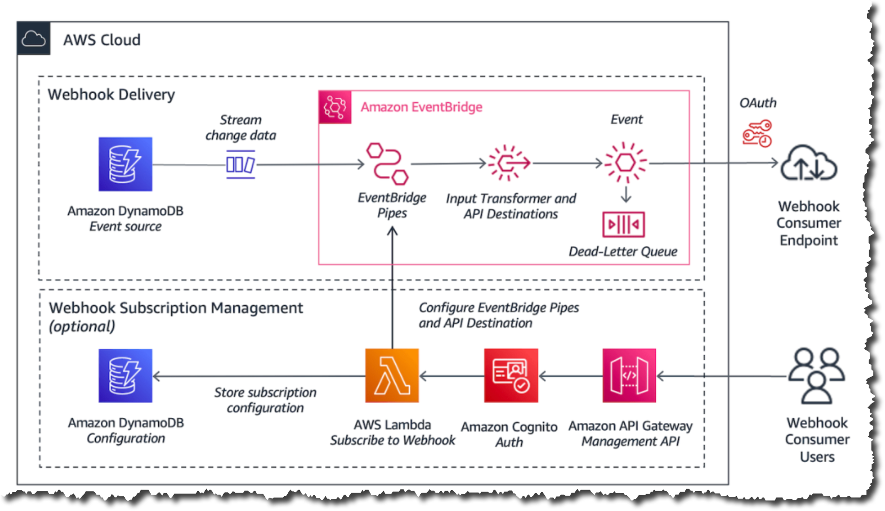
AWS Compute Blog – Daniel Wirjo and Justin Plock wrote a very interesting article about how you can send and receive webhooks on AWS using different AWS serverless services. This is a good read if you are working with webhooks on your application, as it not only shows you how to build these solutions but also what considerations you should have when building them.

AWS Storage Blog – Bimal Gajjar and Andrew Peace wrote a very useful blog post about how to handle event ordering and duplicate events with Amazon S3 Event Notifications. This is a common challenge for many customers.

Amazon Science Blog – David Fan wrote an article about how to build better foundation models for video representation. This article is based on a paper that Prime Video presented at a conference about this topic.

The Official AWS Podcast – Listen each week for updates on the latest AWS news and deep dives into exciting use cases. There are also official AWS podcasts in several languages. Check out the ones in French, German, Italian, and Spanish.

AWS open-source news and updates – This is a newsletter curated by my colleague Ricardo to bring you the latest open source projects, posts, events, and more.

Upcoming AWS events
Check your calendars and sign up for these AWS events:

AWS Community Days – Join a community-led conference run by AWS user group leaders in your region: Ecuador (November 7), Mexico (November 11), Montevideo (November 14), Central Asia (Kazakhstan, Uzbekistan, Kyrgyzstan, and Mongolia on November 17–18), and Guatemala (November 18).

AWS re:Invent (November 27–December 1) – Join us to hear the latest from AWS, learn from experts, and connect with the global cloud community. Browse the session catalog and attendee guides and check out the highlights for generative artificial intelligence (AI).

That’s all for this week. Check back next Monday for another Weekly Roundup!

— Marcia

This post is part of our Weekly Roundup series. Check back each week for a quick roundup of interesting news and announcements from AWS!

Building In-Video Search

Post Syndicated from Netflix Technology Blog original https://netflixtechblog.com/building-in-video-search-936766f0017c

Boris Chen, Ben Klein, Jason Ge, Avneesh Saluja, Guru Tahasildar, Abhishek Soni, Juan Vimberg, Elliot Chow, Amir Ziai, Varun Sekhri, Santiago Castro, Keila Fong, Kelli Griggs, Mallia Sherzai, Robert Mayer, Andy Yao, Vi Iyengar, Jonathan Solorzano-Hamilton, Hossein Taghavi, Ritwik Kumar

Introduction

Today we’re going to take a look at the behind the scenes technology behind how Netflix creates great trailers, Instagram reels, video shorts and other promotional videos.

Suppose you’re trying to create the trailer for the action thriller The Gray Man, and you know you want to use a shot of a car exploding. You don’t know if that shot exists or where it is in the film, and you have to look for it it by scrubbing through the whole film.

Exploding cars — The Gray Man (2022)

Or suppose it’s Christmas, and you want to create a great instagram piece out all the best scenes across Netflix films of people shouting “Merry Christmas”! Or suppose it’s Anya Taylor Joy’s birthday, and you want to create a highlight reel of all her most iconic and dramatic shots.

Making these comes down to finding the right video clips amongst hundreds of thousands movies and TV shows to find the right line of dialogue or the right visual elements (objects, scenes, emotions, actions, etc.). We have built an internal system that allows someone to perform in-video search across the entire Netflix video catalog, and we’d like to share our experience in building this system.

Building in-video search

To build such a visual search engine, we needed a machine learning system that can understand visual elements. Our early attempts included object detection, but found that general labels were both too limiting and too specific, yet not specific enough. Every show has special objects that are important (e.g. Demogorgon in Stranger Things) that don’t translate to other shows. The same was true for action recognition, and other common image and video tasks.

The Approach

We found that contrastive learning between images and text pairs work well for our goals because these models are able to learn joint embedding spaces between the two modalities. This approach is also able to learn about objects, scenes, emotions, actions, and more in a single model. We also found that extending contrastive learning to videos and text provided a substantial improvement over frame-level models.

In order to train the model on internal training data (video clips with aligned text descriptions), we implemented a scalable version on Ray Train and switched to a more performant video decoding library. Lastly, the embeddings from the video encoder exhibit strong zero or few-shot performance on multiple video and content understanding tasks at Netflix and are used as a starting point in those applications.

The recent success of large-scale models that jointly train image and text embeddings has enabled new use cases around multimodal retrieval. These models are trained on large amounts of image-caption pairs via in-batch contrastive learning. For a (large) batch of N examples, we wish to maximize the embedding (cosine) similarity of the N correct image-text pairs, while minimizing the similarity of the other N²-N paired embeddings. This is done by treating the similarities as logits and minimizing the symmetric cross-entropy loss, which gives equal weighting to the two settings (treating the captions as labels to the images and vice versa).

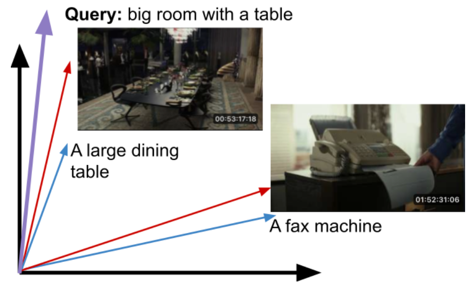
Consider the following two images and captions:

Images are from Glass Onion: A Knives Out Mystery (2022)

Once properly trained, the embeddings for the corresponding images and text (i.e. captions) will be close to each other and farther away from unrelated pairs.

Typically embedding spaces are hundred/thousand dimensional.

At query time, the input text query can be mapped into this embedding space, and we can return the closest matching images.

The query may have not existed in the training set. Cosine similarity can be used as a similarity measure.

While these models are trained on image-text pairs, we have found that they are an excellent starting point to learning representations of video units like shots and scenes. As videos are a sequence of images (frames), additional parameters may need to be introduced to compute embeddings for these video units, although we have found that for shorter units like shots, an unparameterized aggregation like averaging (mean-pooling) can be more effective. To train these parameters as well as fine-tune the pretrained image-text model weights, we leverage in-house datasets that pair shots of varying durations with rich textual descriptions of their content. This additional adaptation step improves performance by 15–25% on video retrieval tasks (given a text prompt), depending on the starting model used and metric evaluated.

On top of video retrieval, there are a wide variety of video clip classifiers within Netflix that are trained specifically to find a particular attribute (e.g. closeup shots, caution elements). Instead of training from scratch, we have found that using the shot-level embeddings can give us a significant head start, even beyond the baseline image-text models that they were built on top of.

Lastly, shot embeddings can also be used for video-to-video search, a particularly useful application in the context of trailer and promotional asset creation.

Engineering and Infrastructure

Our trained model gives us a text encoder and a video encoder. Video embeddings are precomputed on the shot level, stored in our media feature store, and replicated to an elastic search cluster for real-time nearest neighbor queries. Our media feature management system automatically triggers the video embedding computation whenever new video assets are added, ensuring that we can search through the latest video assets.

The embedding computation is based on a large neural network model and has to be run on GPUs for optimal throughput. However, shot segmentation from a full-length movie is CPU-intensive. To fully utilize the GPUs in the cloud environment, we first run shot segmentation in parallel on multi-core CPU machines, store the result shots in S3 object storage encoded in video formats such as mp4. During GPU computation, we stream mp4 video shots from S3 directly to the GPUs using a data loader that performs prefetching and preprocessing. This approach ensures that the GPUs are efficiently utilized during inference, thereby increasing the overall throughput and cost-efficiency of our system.

At query time, a user submits a text string representing what they want to search for. For visual search queries, we use the text encoder from the trained model to extract an text embedding, which is then used to perform appropriate nearest neighbor search. Users can also select a subset of shows to search over, or perform a catalog wide search, which we also support.

If you’re interested in more details, see our other post covering the Media Understanding Platform.

Conclusion

Finding a needle in a haystack is hard. We learned from talking to video creatives who make trailers and social media videos that being able to find needles was key, and a big pain point. The solution we described has been fruitful, works well in practice, and is relatively simple to maintain. Our search system allows our creatives to iterate faster, try more ideas, and make more engaging videos for our viewers to enjoy.

We hope this post has been interesting to you. If you are interested in working on problems like this, Netflix is always hiring great researchers, engineers and creators.


Building In-Video Search was originally published in Netflix TechBlog on Medium, where people are continuing the conversation by highlighting and responding to this story.

The collective thoughts of the interwebz