Post Syndicated from Derrick Stolee original https://github.blog/2022-08-29-gits-database-internals-i-packed-object-store/

Developers collaborate using Git. It is the medium that allows us to share code, work independently on our own machines, and then finally combine our efforts into a common understanding. For many, this is done by following some well-worn steps and sticking to that pattern. This works in the vast majority of use cases, but what happens when we need to do something new with Git? Knowing more about Git’s internals helps when exploring those new solutions.

In this five-part blog post series, we will illuminate Git’s internals to help you collaborate via Git, especially at scale.

It might also be interesting because you love data structures and algorithms. That’s what drives me to be interested in and contribute to Git.

Git’s architecture follows patterns that may be familiar to developers, except the patterns come from a different context. Almost all applications use a database to persist and query data. When building software based on an application database system, it’s easy to get started without knowing any of the internals. However, when it’s time to scale your solution, you’ll have to dive into more advanced features like indexes and query plans.

The core idea I want to convey is this:

Git is the distributed database at the core of your engineering system.

Here are some very basic concepts that Git shares with application databases:

1. Data is persisted to disk.
2. Queries allow users to request information based on that data.
3. The data storage is optimized for these queries.
4. The query algorithms are optimized to take advantage of these structures.
5. Distributed nodes need to synchronize and agree on some common state.

While these concepts are common to all databases, Git is particularly specialized. Git was built to store plain-text source code files, where most change are small enough to read in a single sitting, even if the codebase contains millions of lines. People use Git to store many other kinds of data, such as documentation, web pages, or configuration files.

While many application databases use long-running processes with significant amounts of in-memory caching, Git uses short-lived processes and uses the filesystem to persist data between executions. Git’s data types are more restrictive than a typical application database. These aspects lead to very specialized data storage and access patterns.

Today, let’s dig into the basics of what data Git stores and how it accesses that data. Specifically, we will learn about Git’s object store and how it uses packfiles to compress data that would otherwise contain redundant information.

Git’s object store

The most fundamental concepts in Git are Git objects. These are the “atoms” of your Git repository. They combine in interesting ways to create the larger structure. Let’s start with a quick overview of the important Git objects. Feel free to skip ahead if you know this, or you can dig deep into Git’s object model if you’re interested.

In your local Git repositories, your data is stored in the .git directory. Inside, there is a .git/objects directory that contains your Git objects.

$ ls .git/objects/
01  34  9a  df  info    pack

$ ls .git/objects/01/
12010547a8990673acf08117134bdc181bd735

$ ls .git/objects/pack/
multi-pack-index
pack-7017e6ce443801478cf19006fc5499ba1c4d2960.idx
pack-7017e6ce443801478cf19006fc5499ba1c4d2960.pack
pack-9f9258a8ffe4187f08a93bcba47784e07985d999.idx
pack-9f9258a8ffe4187f08a93bcba47784e07985d999.pack

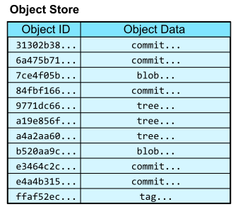
The .git/objects directory is called the object store. It is a content-addressable data store, meaning that we can retrieve the contents of an object by providing a hash of those contents.

In this way, the object store is like a database table with two columns: the object ID and the object content. The object ID is the hash of the object content and acts like a primary key.

Upon first encountering content-addressable data stores, it is natural to ask, “How can we access an object by hash if we don’t already know its content?” We first need to have some starting points to navigate into the object store, and from there we can follow links between objects that exist in the structure of the object data.

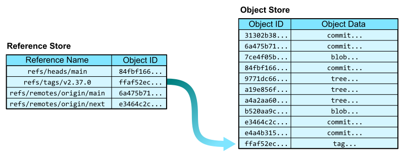
First, Git has references that allow you to create named pointers to keys in the object database. The reference store mainly exists in the .git/refs/ directory and has its own advanced way of storing and querying references efficiently. For now, think of the reference store as a two-column table with columns for the reference name and the object ID. In the reference store, the reference name is the primary key.

Now that we have a reference store, we can navigate into the object store from some human-readable names. In addition to specifying a reference by its full name, such as refs/tags/v2.37.0, we can sometimes use short names, such as v2.37.0 where appropriate.

In the Git codebase, we can start from the v2.37.0 reference and follow the links to each kind of Git object.

• The refs/tags/v2.37.0 reference points to an annotated tag object. An annotated tag contains a reference to another object (by object ID) and a plain-text message.
• That tag’s object references a commit object. A commit is a snapshot of the worktree at a point in time, along with connections to previous versions. It contains links to parent commits, a root tree, as well as metadata, such as commit time and commit message.
• That commit’s root tree references a tree object. A tree is similar to a directory in that it contains entries that link a path name to an object ID.
• From that tree, we can follow the entry for README.md to find a blob object. Blobs store file contents. They get their name from the tree that points to them.

From this example, we navigated from a ref to the contents of the README.md file at that position in the history. This very simple request of “give me the README at this tag” required several hops through the object database, linking an object ID to that object’s contents.

These hops are critical to many interesting Git algorithms. We will explore how the graph structure of the object store is used by Git’s algorithms in parts two through four. For now, let’s focus on the critical operation of linking an object ID to the object contents.

Object store queries

To store and access information in an application database, developers interact with the database using a query language such as SQL. Git has its own type of query language: the command-line interface. Git commands are how we interact with the Git object store. Since Git has its own structure, we do not get the full flexibility of a relational database. However, there are some parallels.

To select object contents by object ID, the git cat-file command will do the object lookup and provide the necessary information. We’ve already been using git cat-file -p to present “pretty” versions of the Git object data by object ID. The raw content is not always fit for human readers, with object IDs stored as raw hashes and not hexadecimal digits, among other things like null bytes. We can also use git cat-file -t to show the type of an object, which is discoverable from the initial few bytes of the object data.

To insert an object into the object store, we can write directly to a blob using git hash-object. This command takes file content and writes it into a blob in the object store. After the input is complete, Git reports the object ID of the written blob.

$ git hash-object -w --stdin
Hello, world!
af5626b4a114abcb82d63db7c8082c3c4756e51b

$ git cat-file -t af5626b4a114abcb82d63db7c8082c3c4756e51b
blob

$ git cat-file -p af5626b4a114abcb82d63db7c8082c3c4756e51b
Hello, world!

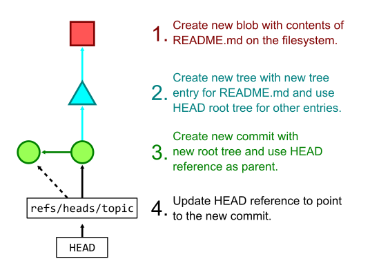
More commonly, we not only add a file’s contents to the object store, but also prepare to create new commit and tree objects to reference that new content. The git add command hashes new changes in the worktree and stores their blobs in the object store then writes the list of objects to a staging area known as the Git index. The git commit command takes those staged changes and creates trees pointing to all of the new blobs, then creates a new commit object pointing to the new root tree. Finally, git commit also updates the current branch to point to the new commit.

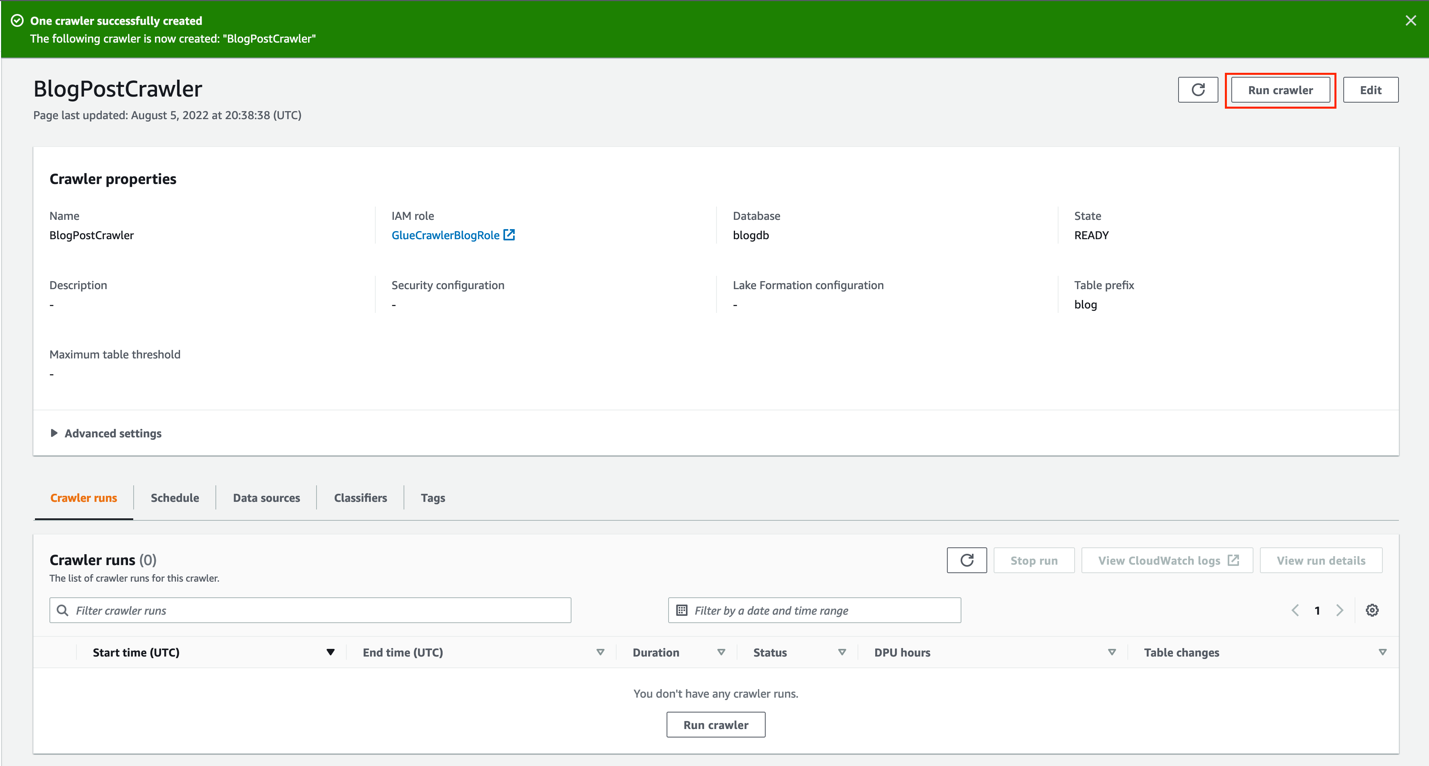
The figure below shows the process of creating several Git objects and finally updating a reference that happens when running git commit -a -m "Update README.md" when the only local edit is a change to the README.md file.

We can do slightly more complicated queries based on object data. Using git log --pretty=format:<format-string>, we can make custom queries into the commits by pulling out “columns” such as the object ID and message, and even the committer and author names, emails, and dates. See the git log documentation for a full column list.

There are also some prebuilt formats ready for immediate use. For example, we can get a simple summary of a commit using git log --pretty=reference -1 <ref>. This query parses the commit at <ref> and provides the following information:

• An abbreviated object ID.
• The first sentence of the commit message.
• The commit date in short form.

$ git log --pretty=reference -1 378b51993aa022c432b23b7f1bafd921b7c43835
378b51993aa0 (gc: simplify --cruft description, 2022-06-19)

Now that we’ve explored some of the queries we can make in Git, let’s dig into the actual storage of this data.

Compressed object storage: packfiles

Looking into the .git/objects directory again, we might see several directories with two-digit names. These directories then contain files with long hexadecimal names. These files are called loose objects, and the filename corresponds to the object ID of an object: the first two hexadecimal characters form the directory name while the rest form the filename. While the files themselves are compressed, there is not much interesting about querying these files, since Git relies on filesystem queries to satisfy most of these needs.

However, it does not take many objects before it is infeasible to store an entire Git repository using only loose objects. Not only does it strain the filesystem to have so many files, it is also inefficient when storing many versions of the same text file. Thus, Git’s packed object store in the .git/objects/pack/ directory forms a more efficient way to store Git objects.

Packfiles and pack-indexes

Each *.pack file in .git/objects/pack/ is called a packfile. Packfiles store multiple objects in compressed forms. Not only is each object compressed individually, they can also be compressed against each other to take advantage of common data.

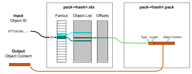
At its simplest, a packfile contains a concatenated list of objects. It only stores the object data, not the object ID. It is possible to read a packfile to find objects by object ID, but it requires decompressing and hashing each object to compare it to the input hash. Instead, each packfile is paired with a pack-index file ending with .idx. The pack-index file stores the list of object IDs in lexicographical order so a quick binary search is sufficient to discover if an object ID is in the packfile, then an offset value points to where the object’s data begins within the packfile. The pack-index operates like a query index that speeds up read queries that rely on the primary key (object ID).

One small optimization is that a fanout table of 256 entries provides boundaries within the full list of object IDs based on their first byte. This reduces the time spent by the binary search, specifically by focusing the search on a smaller number of memory pages. This works particularly well because object IDs are uniformly distributed so the fanout ranges are well-balanced.

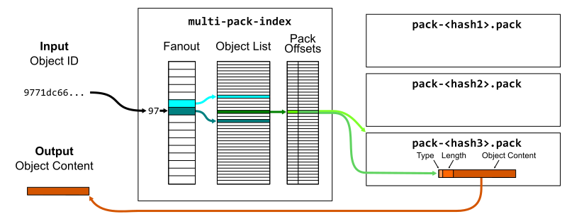
If we have a number of packfiles, then we could ask each pack-index in sequence to look up the object. A further enhancement to packfiles is to put several pack-indexes together in a single multi-pack-index, which stores the same offset data plus which packfile the object is in.

Lookups and prefixes work the same as in pack-indexes, except now we can skip the linear issue with many packs. You can read more about the multi-pack-index file and how it helps scale monorepo maintenance at GitHub.

Diffable object content

Packfiles also have a hyper-specialized version of row compression called deltification. Since read queries are only indexed by the object ID, we can perform extra compression on the object data part.

Git was built to store source code, which consists of plain-text files that are used as input to a compiler or interpreter to create applications. Git was also built to store many versions of this source code as it is changed by humans. This provides additional context about the kind of data typically stored in Git: diffable files with significant portions in common. If you’ve ever wondered why you shouldn’t store large binary files in Git repositories, this is the reason.

The field of software engineering has made it clear that it is difficult to understand applications in their entirety. Humans can grasp a very high-level view of an architecture and can parse small sections of code, but we cannot store enough information in our brains to grasp huge amounts of concrete code at once. You can read more about this in the excellent book, The Programmer’s Brain by Dr. Felienne Hermans.

Because of the limited size of our working memory, it is best to change code in small, well-documented iterations. This helps the code author, any code reviewers, and future developers looking at the code history. Between iterations, a significant majority of the code remains fixed while only small portions change. This allows Git to use difference algorithms to identify small diffs between the content of blob objects.

There are many ways to compute a difference between two blobs. Git has several difference algorithms implemented which can have drastically different results. Instead of focusing on unstructured differences, I want to focus on differences between structured object data. Specifically, tree objects usually change in small ways that are easy to compress.

Tree diffs

Git’s tree objects can also be compared using a difference algorithm that is aware of the structure of tree entries. Each tree entry stores a mode (think Unix file permissions), an object type, a name, and an object ID. Object IDs are for all intents and purposes random, but most edits will change a file without changing its mode, type, or name. Further, large trees are likely to have only a few entries change at a time.

For example, the tip commit at any major Git release only changes one file: the GIT-VERSION-GEN file. This means also that the root tree only has one entry different from the previous root tree:

$ git diff v2.37.0~1 v2.37.0
diff --git a/GIT-VERSION-GEN b/GIT-VERSION-GEN
index 120af376c1..b210b306b7 100755
--- a/GIT-VERSION-GEN
+++ b/GIT-VERSION-GEN
@@ -1,7 +1,7 @@
 #!/bin/sh

 GVF=GIT-VERSION-FILE
-DEF_VER=v2.37.0-rc2
+DEF_VER=v2.37.0

 LF='
 '

$ git cat-file -p v2.37.0~1^{tree} >old
$ git cat-file -p v2.37.0^{tree} >new

$ diff old new
13c13
< 100755 blob 120af376c147799e6c0069bac1f61709a0286cd6  GIT-VERSION-GEN
---
> 100755 blob b210b306b7554f28dc687d1c503517d2a5f87082  GIT-VERSION-GEN

Once we have an algorithm that can compute diffs for Git objects, the packfile format can take advantage of that.

Delta compression

The packfile format begins with some simple header information, but then it contains Git object data concatenated together. Each object’s data starts with a type and a length. The type could be the object type, in which case the content in the packfile is the full object content (subject to DEFLATE compression). The object’s type could instead be an offset delta, in which case the data is based on the content of a previous object in the packfile.

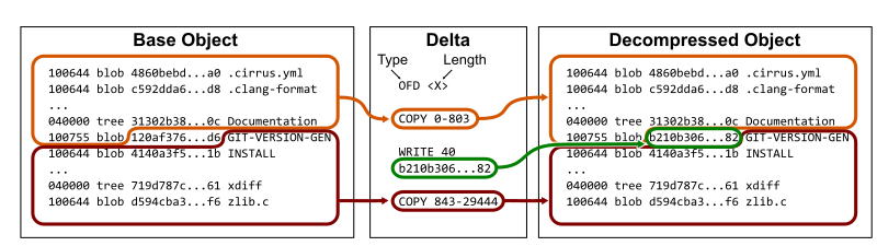
An offset delta begins with an integer offset value pointing to the relative position of a previous object in the packfile. The remaining data specifies a list of instructions which either instruct how to copy data from the base object or to write new data chunks.

Thinking back to our example of the root tree for Git’s v2.37.0 tag, we can store that tree as an offset delta to the previous root tree by copying the tree up until the object ID 120af37..., then write the new object ID b210b30..., and finally copy the rest of the previous root tree.

Keep in mind that these instructions are also DEFLATE compressed, so the new data chunks can also be compressed similarly to the base object. For the example above, we can see that the root tree for v2.37.0 is around 19KB uncompressed, 14KB compressed, but can be represented as an offset delta in only 50 bytes.

$ git rev-parse v2.37.0^{tree}
a4a2aa60ab45e767b52a26fc80a0a576aef2a010

$ git cat-file -s v2.37.0^{tree}
19388

$ ls -al .git/objects/a4/a2aa60ab45e767b52a26fc80a0a576aef2a010
-r--r--r--   1 ... ... 13966 Aug  1 13:24 a2aa60ab45e767b52a26fc80a0a576aef2a010

$ git rev-parse v2.37.0^{tree} | git cat-file --batch-check="%(objectsize:disk)"
50

Also, an offset delta can be based on another object that is also an offset delta. This creates a delta chain that requires computing the object data for each object in the list. In fact, we need to traverse the delta links in order to even determine the object type.

For this reason, there is a cost to storing objects efficiently this way. At read time, we need to do a bit extra work to materialize the raw object content Git needs to parse to satisfy its queries. There are multiple ways that Git tries to optimize this trade-off.

One way Git minimizes the extra work when parsing delta chains is by keeping the delta-chains short. The pack.depth config value specifies an upper limit on how long delta chains can be while creating a packfile. The default limit is 50.

When writing a packfile, Git attempts to use a recent object as the base and order the delta chain in reverse-chronological order. This allows the queries that involve recent objects to have minimum overhead, while the queries that involve older objects have slightly more overhead.

However, while thinking about the overhead of computing object contents from a delta chain, it is important to think about what kind of resources are being used. For example, to compute the diff between v2.37.0 and its parent, we need to load both root trees. If these root trees are in the same delta chain, then that chain’s data on disk is smaller than if they were stored in raw form. Since the packfile also places delta chains in adjacent locations in the packfile, the cost of reading the base object and its delta from disk is almost identical to reading just the base object. The extra overhead of some CPU during the parse is very small compared to the disk read. In this way, reading multiple objects in the same delta chain is faster than reading multiple objects across different chains.

In addition, some Git commands query the object store in such a way that we are very likely to parse multiple objects in the same delta chain. We will cover this more in part III when discussing file history queries.

In addition to persisting data efficiently to disk, the packfile format is also critical to how Git synchronizes Git object data across distributed copies of the repository during git fetch and git push. We will learn more about this in part IV when discussing distributed synchronization.

Packfile maintenance

In order to take advantage of packfiles and their compressed representation of Git objects, Git needs to actually write these packfiles. It is too expensive to create a packfile for every object write, so Git batches the packfile write into certain commands.

You could roll your own packfile using git pack-objects and create a pack-index for it using git index-pack. However, you instead might want to recompute a new packfile containing your entire object store using git repack -a or git gc.

As your repository grows, it becomes more difficult to replace your entire object store with a new packfile. For starters, you need enough space to store two copies of your Git object data. In addition, the computation effort to find good delta compression is very expensive and demanding. An optimal way to do delta compression takes quadratic time over the number objects, which is quickly infeasible. Git uses several heuristics to help with this, but still the cost of repacking everything all at once can be more than we are willing to spend, especially if we are just a client repository and not responsible for serving our Git data to multiple users.

There are two primary ways to update your object store for efficient reads without rewriting the entire object store into a new packfile. One is the geometric repacking option where you can run git repack --geometric to repack only a portion of packfiles until the resulting packfiles form a geometric sequence. That is, each packfile is some fixed multiple smaller than the next largest one. This uses the multi-pack-index to keep logarithmic performance for object lookups, but will occasionally tip over to repack all of the object data. That “tip over” moment only happens when the repository doubles in size, which does not happen very often.

Another approach to reducing the amount of work spent repacking is the incremental repack task in the git maintenance command. This task collects packfiles below a fixed size threshold and groups them together, at least until their total size is above that threshold. The default threshold is two gigabytes. This task is used by default when you enable background maintenance with the git maintenance start command. This also uses the multi-pack-index to keep fast lookups, but also will not rewrite the entire object store for large repositories since once a packfile is larger than the threshold it is not considered for repacking. The storage is slightly inefficient here, since objects in newer packfiles could be stored as deltas to objects in those fixed packs, but the simplicity in avoiding expensive repository maintenance is worth that slight overhead.

If you’re interested in keeping your repositories well maintained, then think about these options. You can always perform a full repack that recomputes all delta chains using git repack -adf at any time you are willing to spend that upfront maintenance cost.

What could Git learn from other databases?

Now that we have some understanding about how Git stores and accesses packed object data, let’s think about features that exist in application database systems that might be helpful here.

One thing to note is that there are no B-trees to be found! Almost every database introduction talks about how B-trees are used to efficiently index data in a database table. Why are they not present here in Git?

The main reason Git does not use B-trees is because it doesn’t do “live updating” of packfiles and pack-indexes. Once a packfile is written, it is static until it is replaced by another packfile containing its objects. That packfile is also not accessed by Git processes until its pack-index is completely written.

In this world, objects are dynamically added to the object store by adding new loose object files (such as in git add or git commit) or by adding new packfiles (such as in git fetch). If a packfile has fixed content, then we can do the most space-and-time efficient index: a binary search tree. Specifically, performing binary search on the list of object IDs in a pack-index is very efficient. It’s not an exact binary search because there is an initial fan-out table for the first byte of the object ID. It’s kind of like a rooted binary tree, except the root node has 256 children instead of only two.

B-trees excel when data is being inserted or removed from the tree. Being able to track those modifications with minimal modifications to the overall tree structure is critical for an application database serving many concurrent requests.

Git does not currently have the capability to update a packfile in real time without shutting down concurrent reads from that file. Such a change could be possible, but it would require updating Git’s storage significantly. I think this is one area where a database expert could contribute to the Git project in really interesting ways.

Another difference between Git and most database systems is that Git runs as short-lived processes. Typically, we think of the database as a process that has data cached in memory. We send queries to the existing process and it returns results and keeps running. Instead, Git starts a new process with every “query” and relies on the filesystem for persisted state. Git also relies on the operating system to cache the disk pages during and between the processes. Expert database systems tell the kernel to stop managing disk pages and instead the database manages the page cache since it knows its usage needs better than a general purpose operating system could predict.

What if Git had a long-running daemon that could satisfy queries on-demand, but also keep that in-memory representation of data instead of needing to parse objects from disk every time? Although the current architecture of Git is not well-suited to this, I believe it is an idea worth exploring in the future.

Come back tomorrow for more!

In the next part of this blog series, we will explore how Git commit history queries use the structure of Git commits to present interesting information to the user. We’ll also explore the commit-graph file and how it acts as a specialized query index for these commands.

I’ll also be speaking at Git Merge 2022 covering all five parts of this blog series, so I look forward to seeing you there!