Post Syndicated from original https://xkcd.com/2645/

Post Syndicated from original https://xkcd.com/2645/
Post Syndicated from original https://lwn.net/Articles/900739/
Back in April, there was an interesting discussion on the python-ideas
mailing list that started as a query about adding support for custom
literals, a la C++, but branched off from there. Custom literals are
frequently used for handling units and unit conversion in C++, so the
Python discussion fairly quickly focused on that use case. While ideas about a
possible feature were batted about, it does not seem like anything that is
being pursued in earnest, at least at this point. But some of the facets
of the problem are, perhaps surprisingly, more complex than might be guessed.
Post Syndicated from Romit Girdhar original https://aws.amazon.com/blogs/big-data/introducing-embedded-analytics-data-lab-to-accelerate-integration-of-amazon-quicksight-analytics-into-applications/
We are excited to announce Embedded Analytics Data Lab (EADL), a no-cost collaborative engagement that helps engineering and development teams cut down time required to launch applications with embedded analytics from Amazon QuickSight in production by providing hands-on guidance and architectural best practices.
Embedding rich analytics such as interactive visuals and dashboards directly into applications allows developers to create differentiated, analytics-driven experiences that enables end-users to make more informed decisions. QuickSight is a cloud-native, serverless business intelligence (BI) service that allows developers from enterprises and independent software vendors (ISVs) to incorporate powerful BI capabilities such as interactive visualizations, dashboards, and machine learning (ML)-powered natural language query (NLQ) using Amazon QuickSight Q into their applications and web portals, delivering insights to end-users where they are.
AWS Data Lab is an AWS offering that offers accelerated, joint engineering engagements between customers and AWS technical resources to create tangible deliverables that accelerate data, analytics, AI/ML, serverless, and containers modernization initiatives.
Today, with the new EADL offering, we’re bringing together the breadth of QuickSight’s embedding capabilities with proven expertise from AWS Data Lab. With EADL, AWS customers can request a hands-on session to prototype embedded analytics solutions, build custom architectures, and implement best practices with QuickSight-specialist Data Lab Solutions Architects. The output from this engagement is a customized solution that is specific to customer requirements, built using their data, in their AWS account, while providing hands-on learning to the engineering teams attending the lab. EADL engagements accelerate time from ideation to proof of concept to production by months, through tailored guidance while using resources across AWS teams to accelerate the rollout of embedded analytics features powered by QuickSight.
“We’re excited to announce the launch of the Embedded Analytics Data Lab that enables customers and ISVs to accelerate their embedded analytics offering using Amazon QuickSight. With Amazon QuickSight’s embedded analytics capabilities, AWS customers can integrate rich visuals and dashboards into their applications to scale to 100,000s of end-users, differentiating their user experiences—without any servers or infrastructure management. Embedded Analytics Data Lab helps demonstrate this business value in a matter of days by accelerating the QuickSight embedded journey for development teams.”
– Tracy Daugherty, General Manager, Amazon QuickSight.
Customers in EADL work closely with assigned AWS Data Lab Solutions Architect, solidifying the architecture design for their embedded analytics solution, including designing any data model and data pipeline components. The engagement then proceeds to the lab phase, where builders spend 2–4 days with their Solutions Architect, working backward from end goals and building a solution based on the previously defined architecture and real-time guidance from the Solutions Architect and other AWS service experts. Data Lab Solutions Architects also provide implementation guidance on data modeling, setting up multi-tenancy, enabling single sign-on with customers’ identity providers, enabling row- and column-level security, and tracking the health of the QuickSight environment. At lab completion, customers leave with a working prototype of their embedded analytics solution, built by their own builders in their AWS accounts that meet their requirements and specs.
Over the last year, we have worked closely with customers to help design and build their embedded analytics solutions. Some of these customers include BriteCore, Carbyne, and KRS.io.
 |
BriteCore is an enterprise-level insurance processing suite that relies on dashboards to provide operational tracking and trend insights to insurance carriers on data points such as insurance claims and losses by agency, policy type, and line of business. To provide a seamless experience for their over 125,000 customers, BriteCore sought to integrate their BI offerings with their core platform and deliver dashboards to customers as embedded visuals. BriteCore’s engineering and reporting and analytics teams engaged the AWS Data Lab to design and validate the best integration approach between QuickSight and their application and to jumpstart building their interactive, embedded QuickSight dashboards. |
“AWS Data Lab was pivotal in helping us build out our embedded analytics solution with the AWS suite of analytics services. Within 4 days, we built a working prototype of our multi-tenant solution with the right identity and security policies in place. Engaging with AWS Data Lab to build our solution definitely helped us reduce our time to production. Our customers now have even better insights into their business, and we will be able to deliver a much richer experience.”
– Supreet Oberoi, Senior Vice President of Engineering, BriteCore.
 |
Carbyne is the global leader in contact center solutions, enabling emergency contact centers and selected enterprises to connect with callers on any connected devices via highly secure communication channels without downloading a consumer app. Carbyne worked with AWS Data Lab to explore options for building a low-latency, multi-tenant analytical system that would enable them to generate meaningful insights using QuickSight’s interactive dashboards for call center owners who manage 911 calls. Example insights include 911 call duration ranges, peak time of day for callers, and percentage of abandoned vs. answered calls—all data points that help Carbyne customers measure the effectiveness of their emergency response systems and then provision staff and resources accordingly. These insights were then embedded into their application, enabling a seamless experience for the 911 call center managers. |
“This experience with the AWS Data Lab is what it means to be in true partnership. Data Lab’s support and efforts are much appreciated as we push innovative solutions to the public safety industry. I can say confidently that Data Lab’s support will reduce our time to production by weeks, if not months.”
– Alex Dizengof, Founder & CTO, Carbyne, Inc.
 |
KRS.io is a leader in coalition loyalty marketing connecting thousands of retailers with their customers on an intimate level with rewards programs and loyalty solutions. To truly democratize data, they set out to build a solution that harnesses the power of NQL. In a 1-day workshop with the AWS Data Lab team, KRS.io embedded QuickSight Q into Epiphany and successfully modeled 20 questions for their Profit Central back office accounting system, perpetual inventory, and loyalty datasets. |
“In business, speed matters. Working with AWS Data Lab accelerated our timeframe from proof of concept to deployment. I had zero-tolerance for risk and the Data Lab allowed my team to meet my high bar for security and reliability”
– Brian McManus, CTO, KRS.io.
Prerequisites required to qualify for this offering are:
|
To get started, register now. Once registered, a member of the AWS team will contact you with next steps. |
 Romit Girdhar manages Technical Product Management & Software Development teams for AWS Data Lab. He focuses on working backwards from customer outcomes to help accelerate their cloud journey. Romit has over a decade of experience working on engineering solutions for and with customers across two major public cloud companies – Amazon and Microsoft.
 Kareem Syed-Mohammed is a Product Manager at Amazon QuickSight. He focuses on embedded analytics, APIs, and developer experience. Prior to QuickSight he has been with AWS Marketplace and Amazon retail as a PM. Kareem started his career as a developer and then PM for call center technologies, Local Expert and Ads for Expedia. He worked as a consultant with McKinsey and Company for a short while.
Post Syndicated from Greg Wiseman original https://blog.rapid7.com/2022/07/12/patch-tuesday-july-2022/

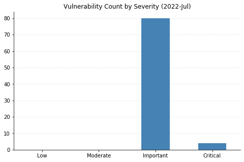
Microsoft’s updates for July’s Patch Tuesday fix 86 CVEs, including two vulnerabilities in their Chromium-based Edge browser that were patched earlier in the month.
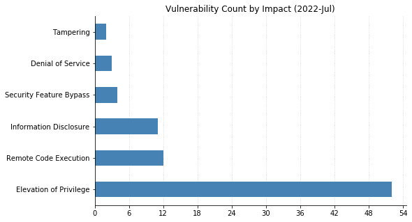
One 0-day vulnerability has been patched: CVE-2022-22047 affects all currently supported versions of Microsoft’s pervasive operating system. This is an elevation-of-privilege vulnerability in the Windows Client Server Runtime Subsystem (CSRSS), a critical service that is often impersonated by malware. An attacker with an already-existing foothold can exploit this vulnerability to gain SYSTEM-level privileges. Two similar vulnerabilities in CSRSS (CVE-2022-22049 and CVE-2022-22026) were also fixed, likely as a result of Microsoft’s investigation into the in-the-wild exploitation of CVE-2022-22047.
Four critical remote code execution (RCE) vulnerabilities were fixed today. CVE-2022-22029 and CVE-2022-22039 affect network file system (NFS) servers, and CVE-2022-22038 affects the remote procedure call (RPC) runtime. Although all three of these will be relatively tricky for attackers to exploit due to the amount of sustained data that needs to be transmitted, administrators should patch sooner rather than later. CVE-2022-30221 supposedly affects the Windows Graphics Component, though Microsoft’s FAQ indicates that exploitation requires users to access a malicious RDP server.
Over a third of today’s vulnerabilities (a whopping 32 CVEs) affect their Azure Site Recovery offering. Anyone making use of this VMWare-to-Azure backup solution should be sure to upgrade to version 9.49 of the Microsoft Azure Site Recovery Unified Setup, available in Update rollup 62.

| CVE | Title | Exploited? | Publicly disclosed? | CVSSv3 base score | Has FAQ? |
|---|---|---|---|---|---|
| CVE-2022-33676 | Azure Site Recovery Remote Code Execution Vulnerability | No | No | 7.2 | Yes |
| CVE-2022-33678 | Azure Site Recovery Remote Code Execution Vulnerability | No | No | 7.2 | Yes |
| CVE-2022-33674 | Azure Site Recovery Elevation of Privilege Vulnerability | No | No | 8.3 | Yes |
| CVE-2022-33675 | Azure Site Recovery Elevation of Privilege Vulnerability | No | No | 7.8 | Yes |
| CVE-2022-33677 | Azure Site Recovery Elevation of Privilege Vulnerability | No | No | 7.2 | Yes |
| CVE-2022-30181 | Azure Site Recovery Elevation of Privilege Vulnerability | No | No | 6.5 | Yes |
| CVE-2022-33641 | Azure Site Recovery Elevation of Privilege Vulnerability | No | No | 6.5 | Yes |
| CVE-2022-33643 | Azure Site Recovery Elevation of Privilege Vulnerability | No | No | 6.5 | Yes |
| CVE-2022-33655 | Azure Site Recovery Elevation of Privilege Vulnerability | No | No | 6.5 | Yes |
| CVE-2022-33656 | Azure Site Recovery Elevation of Privilege Vulnerability | No | No | 6.5 | Yes |
| CVE-2022-33657 | Azure Site Recovery Elevation of Privilege Vulnerability | No | No | 6.5 | Yes |
| CVE-2022-33661 | Azure Site Recovery Elevation of Privilege Vulnerability | No | No | 6.5 | Yes |
| CVE-2022-33662 | Azure Site Recovery Elevation of Privilege Vulnerability | No | No | 6.5 | Yes |
| CVE-2022-33663 | Azure Site Recovery Elevation of Privilege Vulnerability | No | No | 6.5 | Yes |
| CVE-2022-33665 | Azure Site Recovery Elevation of Privilege Vulnerability | No | No | 6.5 | Yes |
| CVE-2022-33666 | Azure Site Recovery Elevation of Privilege Vulnerability | No | No | 6.5 | Yes |
| CVE-2022-33667 | Azure Site Recovery Elevation of Privilege Vulnerability | No | No | 6.5 | Yes |
| CVE-2022-33672 | Azure Site Recovery Elevation of Privilege Vulnerability | No | No | 6.5 | Yes |
| CVE-2022-33673 | Azure Site Recovery Elevation of Privilege Vulnerability | No | No | 6.5 | Yes |
| CVE-2022-33642 | Azure Site Recovery Elevation of Privilege Vulnerability | No | No | 4.9 | Yes |
| CVE-2022-33650 | Azure Site Recovery Elevation of Privilege Vulnerability | No | No | 4.9 | Yes |
| CVE-2022-33651 | Azure Site Recovery Elevation of Privilege Vulnerability | No | No | 4.9 | Yes |
| CVE-2022-33653 | Azure Site Recovery Elevation of Privilege Vulnerability | No | No | 4.9 | Yes |
| CVE-2022-33654 | Azure Site Recovery Elevation of Privilege Vulnerability | No | No | 4.9 | Yes |
| CVE-2022-33659 | Azure Site Recovery Elevation of Privilege Vulnerability | No | No | 4.9 | Yes |
| CVE-2022-33660 | Azure Site Recovery Elevation of Privilege Vulnerability | No | No | 4.9 | Yes |
| CVE-2022-33664 | Azure Site Recovery Elevation of Privilege Vulnerability | No | No | 4.9 | Yes |
| CVE-2022-33668 | Azure Site Recovery Elevation of Privilege Vulnerability | No | No | 4.9 | Yes |
| CVE-2022-33669 | Azure Site Recovery Elevation of Privilege Vulnerability | No | No | 4.9 | Yes |
| CVE-2022-33671 | Azure Site Recovery Elevation of Privilege Vulnerability | No | No | 4.9 | Yes |
| CVE-2022-33652 | Azure Site Recovery Elevation of Privilege Vulnerability | No | No | 4.4 | Yes |
| CVE-2022-33658 | Azure Site Recovery Elevation of Privilege Vulnerability | No | No | 4.4 | Yes |
| CVE | Title | Exploited? | Publicly disclosed? | CVSSv3 base score | Has FAQ? |
|---|---|---|---|---|---|
| CVE-2022-30187 | Azure Storage Library Information Disclosure Vulnerability | No | No | 4.7 | Yes |
| CVE | Title | Exploited? | Publicly disclosed? | CVSSv3 base score | Has FAQ? |
|---|---|---|---|---|---|
| CVE-2022-2295 | Chromium: CVE-2022-2295 Type Confusion in V8 | No | No | N/A | Yes |
| CVE-2022-2294 | Chromium: CVE-2022-2294 Heap buffer overflow in WebRTC | No | No | N/A | Yes |
| CVE | Title | Exploited? | Publicly disclosed? | CVSSv3 base score | Has FAQ? |
|---|---|---|---|---|---|
| CVE-2022-33633 | Skype for Business and Lync Remote Code Execution Vulnerability | No | No | 7.2 | Yes |
| CVE-2022-33632 | Microsoft Office Security Feature Bypass Vulnerability | No | No | 4.7 | Yes |
| CVE | Title | Exploited? | Publicly disclosed? | CVSSv3 base score | Has FAQ? |
|---|---|---|---|---|---|
| CVE-2022-33637 | Microsoft Defender for Endpoint Tampering Vulnerability | No | No | 6.5 | Yes |
| CVE | Title | Exploited? | Publicly disclosed? | CVSSv3 base score | Has FAQ? |
|---|---|---|---|---|---|
| CVE-2022-33644 | Xbox Live Save Service Elevation of Privilege Vulnerability | No | No | 7 | Yes |
| CVE-2022-22045 | Windows.Devices.Picker.dll Elevation of Privilege Vulnerability | No | No | 7.8 | Yes |
| CVE-2022-30222 | Windows Shell Remote Code Execution Vulnerability | No | No | 8.4 | Yes |
| CVE-2022-30216 | Windows Server Service Tampering Vulnerability | No | No | 8.8 | Yes |
| CVE-2022-22041 | Windows Print Spooler Elevation of Privilege Vulnerability | No | No | 6.8 | Yes |
| CVE-2022-30214 | Windows DNS Server Remote Code Execution Vulnerability | No | No | 6.6 | Yes |
| CVE-2022-22031 | Windows Credential Guard Domain-joined Public Key Elevation of Privilege Vulnerability | No | No | 7.8 | Yes |
| CVE-2022-30212 | Windows Connected Devices Platform Service Information Disclosure Vulnerability | No | No | 4.7 | Yes |
| CVE-2022-22711 | Windows BitLocker Information Disclosure Vulnerability | No | No | 6.7 | Yes |
| CVE-2022-22038 | Remote Procedure Call Runtime Remote Code Execution Vulnerability | No | No | 8.1 | Yes |
| CVE-2022-27776 | HackerOne: CVE-2022-27776 Insufficiently protected credentials vulnerability might leak authentication or cookie header data | No | No | N/A | Yes |
| CVE-2022-30215 | Active Directory Federation Services Elevation of Privilege Vulnerability | No | No | 7.5 | Yes |
| CVE | Title | Exploited? | Publicly disclosed? | CVSSv3 base score | Has FAQ? |
|---|---|---|---|---|---|
| CVE-2022-30208 | Windows Security Account Manager (SAM) Denial of Service Vulnerability | No | No | 6.5 | No |
| CVE-2022-30206 | Windows Print Spooler Elevation of Privilege Vulnerability | No | No | 7.8 | Yes |
| CVE-2022-30226 | Windows Print Spooler Elevation of Privilege Vulnerability | No | No | 7.1 | Yes |
| CVE-2022-22022 | Windows Print Spooler Elevation of Privilege Vulnerability | No | No | 7.1 | Yes |
| CVE-2022-22023 | Windows Portable Device Enumerator Service Security Feature Bypass Vulnerability | No | No | 6.6 | Yes |
| CVE-2022-22029 | Windows Network File System Remote Code Execution Vulnerability | No | No | 8.1 | Yes |
| CVE-2022-22039 | Windows Network File System Remote Code Execution Vulnerability | No | No | 7.5 | Yes |
| CVE-2022-22028 | Windows Network File System Information Disclosure Vulnerability | No | No | 5.9 | Yes |
| CVE-2022-30225 | Windows Media Player Network Sharing Service Elevation of Privilege Vulnerability | No | No | 7.1 | Yes |
| CVE-2022-30211 | Windows Layer 2 Tunneling Protocol (L2TP) Remote Code Execution Vulnerability | No | No | 7.5 | Yes |
| CVE-2022-21845 | Windows Kernel Information Disclosure Vulnerability | No | No | 4.7 | Yes |
| CVE-2022-22025 | Windows Internet Information Services Cachuri Module Denial of Service Vulnerability | No | No | 7.5 | No |
| CVE-2022-30209 | Windows IIS Server Elevation of Privilege Vulnerability | No | No | 7.4 | Yes |
| CVE-2022-22042 | Windows Hyper-V Information Disclosure Vulnerability | No | No | 6.5 | Yes |
| CVE-2022-30223 | Windows Hyper-V Information Disclosure Vulnerability | No | No | 5.7 | Yes |
| CVE-2022-30205 | Windows Group Policy Elevation of Privilege Vulnerability | No | No | 6.6 | Yes |
| CVE-2022-30221 | Windows Graphics Component Remote Code Execution Vulnerability | No | No | 8.8 | Yes |
| CVE-2022-22034 | Windows Graphics Component Elevation of Privilege Vulnerability | No | No | 7.8 | Yes |
| CVE-2022-30213 | Windows GDI+ Information Disclosure Vulnerability | No | No | 5.5 | Yes |
| CVE-2022-22024 | Windows Fax Service Remote Code Execution Vulnerability | No | No | 7.8 | Yes |
| CVE-2022-22027 | Windows Fax Service Remote Code Execution Vulnerability | No | No | 7.8 | Yes |
| CVE-2022-22050 | Windows Fax Service Elevation of Privilege Vulnerability | No | No | 7.8 | Yes |
| CVE-2022-22043 | Windows Fast FAT File System Driver Elevation of Privilege Vulnerability | No | No | 7.8 | Yes |
| CVE-2022-30220 | Windows Common Log File System Driver Elevation of Privilege Vulnerability | No | No | 7.8 | Yes |
| CVE-2022-22026 | Windows CSRSS Elevation of Privilege Vulnerability | No | No | 8.8 | Yes |
| CVE-2022-22047 | Windows CSRSS Elevation of Privilege Vulnerability | Yes | No | 7.8 | Yes |
| CVE-2022-22049 | Windows CSRSS Elevation of Privilege Vulnerability | No | No | 7.8 | Yes |
| CVE-2022-30203 | Windows Boot Manager Security Feature Bypass Vulnerability | No | No | 7.4 | Yes |
| CVE-2022-22037 | Windows Advanced Local Procedure Call Elevation of Privilege Vulnerability | No | No | 7.5 | Yes |
| CVE-2022-30202 | Windows Advanced Local Procedure Call Elevation of Privilege Vulnerability | No | No | 7 | Yes |
| CVE-2022-30224 | Windows Advanced Local Procedure Call Elevation of Privilege Vulnerability | No | No | 7 | Yes |
| CVE-2022-22036 | Performance Counters for Windows Elevation of Privilege Vulnerability | No | No | 7 | Yes |
| CVE-2022-22040 | Internet Information Services Dynamic Compression Module Denial of Service Vulnerability | No | No | 7.3 | Yes |
| CVE-2022-22048 | BitLocker Security Feature Bypass Vulnerability | No | No | 6.1 | Yes |
| CVE-2022-23825 | AMD: CVE-2022-23825 AMD CPU Branch Type Confusion | No | No | N/A | Yes |
| CVE-2022-23816 | AMD: CVE-2022-23816 AMD CPU Branch Type Confusion | No | No | N/A | Yes |
Post Syndicated from Courtney Campbell original https://blog.rapid7.com/2022/07/12/the-forecast-is-flipped-flipping-l-d-to-ensure-continuous-growth/

At Rapid7, we staunchly believe that our people are central to upholding our mission and embodying our core values to ultimately drive our customers into a more secure future. For this reason, Rapid7 works tediously to ensure that our Moose have ample opportunities to learn and grow in their careers.
In order to support such development, the People Development team strives to ensure that our programs are not only impactful but also support our Moose to be “Never Done” in their pursuit to have the career experience of their lifetime. Our approach to learning is to “Challenge Convention” through the proactive and consistent iteration of our programs to reflect this ever-changing world. Such evolution is crucial after a forced 2-year remote work experience and Rapid7’s shift to a hybrid workplace.
Let’s travel back to 2018. From a Learning and Development perspective, this year feels like visiting a vastly different universe – one in which exclusively in-person training across a select set of offices, offered a few times a year, was the norm.
At this point in time, Rapid7 offered five soft-skills training courses, designed to introduce participants to best practices of a specific soft skill that supported professional success. The instructor would facilitate the majority of trainings in our Boston office location and then travel to one or two other office locations in order to offer training to participants outside of the hub location. The challenge? This in-person approach did not account for a growing global workforce; we needed to figure out how to keep our programs inclusive and accessible for those outside of Boston. Furthermore, because it intrinsically took time for the instructor to travel to physical office locations to offer these training sessions, there was a lag between the time when the employee needed the training and the time it was delivered to them. Ultimately, this interlude resulted in a delayed, or even missed, opportunity for learning.
Our team also realized that we were standardizing career development by operating under the assumption that each employee should focus narrowly on those five soft skills rather than championing the uniqueness of each Moose’s individual career experiences and the shifting needs of the business. These challenges served as the fuel that propelled us into the future of our “All Moose” learning programs. It was time to align learner needs with those of the business, put our Moose in the driver’s seat of their development, nurture our ever-growing global employee base, and acknowledge the new world of hybrid work. This focus ultimately helped us move away from a one-size-fits-all approach to learning and propel our mission forward.
With in-person trainings on hold, Rapid7 had the space to thoughtfully investigate what the future of learning could look and feel like for “All Moose.” Thus, the Moose GPS was born. The Moose GPS serves as a strategically adapted version of a traditional Individual Development Plan, transformed into a dynamic and collaborative tool. The “GPS” portion of the tool stands for “Growing, Partnering, and Succeeding” because these are all things the Moose will do while completing one! Composed of three steps, the GPS is unique in that it encourages employee ownership, accountability, and managerial partnership around development. No longer is the conversation and action plan initiated and driven solely by a Moose’s manager.
Originally conceived as enablement for the Moose GPS, People Development curated a collection of courses strategically designed to enable Moose to fiercely take ownership of their unique development path, namely, the Continuous Growth Courses. The ethos behind the three-course Continuous Growth Program is to provide employees with the tools, opportunities, and connections necessary to become champions of their development. While the courses mirror the progression of the Moose GPS, the curriculum intentionally focuses on skill-building rather than on the use of the tool itself.
In reflection of our core value “Challenge Convention,” continuously challenging what is for what could be, the Continuous Growth Program would be the focus for the next iteration of Rapid7’s Learning and Development programs.
The collision between our revolutionized learning philosophy and a global pandemic catalyzed a shift into a new realm of learning, one that prioritizes inclusivity, utilizes technology, and rethinks traditional, classroom-based teaching methods. We understood that changes needed to be made in order to ensure business alignment and overall program effectiveness.
Now, in 2022, Rapid7 has catapulted the Continuous Growth Courses even further ahead. This year, we have “flipped” approximately 50% of our content. This shift has enabled us to “scale with soul” and maximize learner accessibility and inclusivity. Flipped learning is an instructional strategy where learners engage in both self-paced and in-classroom learning activities. The program is strategically designed to ensure cross-sectional engagement and enable measurable behavioral shifts. Courses are taught in a cohort model and include both synchronous and asynchronous activities to support scale while striking a balance between individual learners’ schedules and providing opportunities for collaborative learning.
Each of the courses is two weeks long; during these two weeks, learners are first provided with an interactive e-learning where they engage with material on their own time. The e-learning intentionally introduces the learner to the content by mingling text, video, gamification, and knowledge checks in order to seamlessly immerse the learner into the material and maximize engagement. The on-demand nature of this activity permits the Moose to learn flexibly, encouraging them to self-pace around their own schedules.
The material introduced digitally will later be applied in the live session, where participants across the globe are united in one virtual classroom. By the time the participants attend the live session, the familiarity they have gained with the content in the digital learning experience will be practiced and applied in the live session in order to maximize knowledge absorption. The sessions consist of various activities in which learners are put into breakout rooms where they are able to create new, and otherwise unlikely, connections while bonding over the learning experience. We leverage tenured Moose to present on their own experiences with career development in these sessions, enabling us to scale our programs and foster high impact learning. Simultaneously, through our management development programs, our managers are equipped with the same skills and tools to facilitate meaningful development, feedback, and coaching conversations, providing their Moose with space and time for action.
By equipping employees with the necessary skills to be active participants in their development, we not only empower them to raise the bar and become lifelong learners, but we also cyclically feed our culture of continuous learning. These employees cultivate growth mindsets and understand that their individual growth and success is intertwined with, not separate from, our shared organizational growth and success. By providing experiences for our employees to lean into their growth and development through onboarding, Continuous Growth Courses, and a variety of learning resources, we are investing in their future and our shared future.
“I think this program helped me take a step back and really think about my work and how I want to evolve. It’s easy to get caught up in your day to day without really thinking so this course will help me be more intentional in my goals and growth going forward.”
“I found all three modules to be very helpful – it’s not often you’re prompted to sit and reflect on your career, and the prompts were helpful for doing so.”
“This experience has helped me feel more engaged!”
Since the launch of these courses in April, Moose who have enrolled in the course say:
Managers of Moose who have enrolled in the course say:
This is the final blog post in our series, “The Forecast Is Flipped.” Thank you so much for following along with Rapid7’s innovative learning practices!
Additional reading:
Post Syndicated from original https://lwn.net/Articles/900917/
Some researchers at ETH Zurich have disclosed a
new set of speculative-execution vulnerabilities known as “Retbleed”. In
short, the retpoline defenses added when Spectre was initially disclosed
turn out to be insufficient on x86 machines because return instructions,
too, can be speculatively executed.
Kernel and hypervisor developers have developed mitigations in
coordination with Intel and AMD. Mitigating Retbleed in the Linux
kernel required a substantial effort, involving changes to 68
files, 1783 new lines and 387 removed lines. Our performance
evaluation shows that mitigating Retbleed has unfortunately turned
out to be expensive: we have measured between 14% and 39% overhead
with the AMD and Intel patches respectively.
Those mitigations were pulled into the mainline
kernel today. They are
not in the July 12 stable kernel
updates but will almost certainly show up in those channels soon.
Post Syndicated from Adam Gatt original https://aws.amazon.com/blogs/big-data/optimize-your-amazon-redshift-query-performance-with-automated-materialized-views/
Amazon Redshift is a fast, fully managed cloud data warehouse database that makes it cost-effective to analyze your data using standard SQL and business intelligence tools. Amazon Redshift allows you to analyze structured and semi-structured data and seamlessly query data lakes and operational databases, using AWS designed hardware and automated machine learning (ML)-based tuning to deliver top-tier price-performance at scale.
Although Amazon Redshift provides excellent price performance out of the box, it offers additional optimizations that can improve this performance and allow you to achieve even faster query response times from your data warehouse.
For example, you can physically tune tables in a data model to minimize the amount of data scanned and distributed within a cluster, which speeds up operations such as table joins and range-bound scans. Amazon Redshift now automates this tuning with the automatic table optimization (ATO) feature.
Another optimization for reducing query runtime is to precompute query results in the form of a materialized view. Materialized views store precomputed query results that future similar queries can use. This improves query performance because many computation steps can be skipped and the precomputed results returned directly. Unlike a simple cache, many materialized views can be incrementally refreshed when DML changes are applied on the underlying (base) tables and can be used by other similar queries, not just the query used to create the materialized view.
Amazon Redshift introduced materialized views in March 2020. In June 2020, support for external tables was added. With these releases, you could use materialized views on both local and external tables to deliver low-latency performance by using precomputed views in your queries. However, this approach required you to be aware of what materialized views were available on the cluster, and if they were up to date.
In November 2020, materialized view automatic refresh and query rewrite features were added. With materialized view-aware automatic rewriting, data analysts get the benefit of materialized views for their queries and dashboards without having to query the materialized view directly. The analyst may not even be aware the materialized views exist. The auto rewrite feature enables this by rewriting queries to use materialized views without the query needing to explicitly reference them. In addition, auto refresh keeps materialized views up to date when base table data is changed, and there are available cluster resources for the materialized view maintenance.
However, materialized views still have to be manually created, monitored, and maintained by data engineers or DBAs. To reduce this overhead, Amazon Redshift has introduced the Automated Materialized View (AutoMV) feature, which goes one step further and automatically creates materialized views for queries with common recurring joins and aggregations.
This post explains what materialized views are, how manual materialized views work and the benefits they provide, and what’s required to build and maintain manual materialized views to achieve performance improvements and optimization. Then we explain how this is greatly simplified with the new automated materialized view feature.
A materialized view is a database object that stores precomputed query results in a materialized (persisted) dataset. Similar queries can use the precomputed results from the materialized view and skip the expensive tasks of reading the underlying tables and performing joins and aggregates, thereby improving the query performance.
For example, you can improve the performance of a dashboard by materializing the results of its queries into a materialized view or multiple materialized views. When the dashboard is opened or refreshed, it can use the precomputed results from the materialized view instead of rereading the base tables and reprocessing the queries. By creating a materialized view once and querying it multiple times, redundant processing can be avoided, improving query performance and freeing up resources for other processing on the database.
To demonstrate this, we use the following query, which returns daily order and sales numbers. It joins two tables and aggregates at the day level.
At the top of the query, we set enable_result_cache_for_session to OFF. This setting disables the results cache, so we can see the full processing runtime each time we run the query. Unlike a materialized view, the results cache is a simple cache that stores the results of a single query in memory, it can’t be used by other similar queries, is not updated when the base tables are modified, and because it isn’t persisted, can be aged-out of memory by more frequently used queries.
When we run this query on a 10-node ra3.4xl cluster with the TPC-H 3 TB dataset, it returns in approximately 20 seconds. If we need to run this query or similar queries more than once, we can create a materialized view with the CREATE MATERIALIZED VIEW command and query the materialized view object directly, which has the same structure as a table:
Because the join and aggregations have been precomputed, it runs in approximately 900 milliseconds, a performance improvement of 96%.
As we have just shown, you can query the materialized view directly; however, Amazon Redshift can automatically rewrite a query to use one or more materialized views. The query rewrite feature transparently rewrites the query as it’s being run to retrieve precomputed results from a materialized view. This process is automatically triggered on eligible and up-to-date materialized views, if the query contains the same base tables and joins, and has similar aggregations as the materialized view.
For example, if we rerun the sales query, because it’s eligible for rewriting, it’s automatically rewritten to use the mv_daily_sales materialized view. We start with the original query:
Internally, the query is rewritten to the following SQL and run. This process is completely transparent to the user.
The rewriting can be confirmed by looking at the query’s explain plan:
The plan shows the query has been rewritten and has retrieved the results from the mv_daily_sales materialized view, not the query’s base tables: orders and lineitem.
Other queries that use the same base tables and level of aggregation, or a level of aggregation derived from the materialized view’s level, are also rewritten. For example:
If data in the orders or lineitem table changes, mv_daily_sales becomes stale; this means the materialized view isn’t reflecting the state of its base tables. If we update a row in lineitem and check the stv_mv_info system table, we can see the is_stale flag is set to t (true):
We can now manually refresh the materialized view using the REFRESH MATERIALIZED VIEW statement:
There are two types of materialized view refresh: full and incremental. A full refresh reruns the underlying SQL statement and rebuilds the whole materialized view. An incremental refresh only updates specific rows affected by the source data change. To see if a materialized view is eligible for incremental refreshes, view the state column in the stv_mv_info system table. A state of 0 indicates the materialized view will be fully refreshed, and a state of 1 indicates the materialized view will be incrementally refreshed.
You can schedule manual refreshes on the Amazon Redshift console if you need to refresh a materialized view at fixed periods, such as once per hour. For more information, refer to Scheduling a query on the Amazon Redshift console.
As well as the ability to do a manual refresh, Amazon Redshift can also automatically refresh materialized views. The auto refresh feature intelligently determines when to refresh the materialized view, and if you have multiple materialized views, which order to refresh them in. Amazon Redshift considers the benefit of refreshing a materialized view (how often the materialized view is used, what performance gain the materialized view provides) and the cost (resources required for the refresh, current system load, available system resources).
This intelligent refreshing has a number of benefits. Because not all materialized views are equally important, deciding when and in which order to refresh materialized views on a large system is a complex task for a DBA to solve. Also, the DBA needs to consider other workloads running on the system, and try to ensure the latency of critical workloads is not increased by the effect of refreshing materialized views. The auto refresh feature helps remove the need for a DBA to do these difficult and time-consuming tasks.
You can set a materialized view to be automatically refreshed in the CREATE MATERIALIZED VIEW statement with the AUTO REFRESH YES parameter:
Now when the source data of the materialized view changes, the materialized view is automatically refreshed. We can view the status of the refresh in the svl_mv_refresh_status system table. For example:
To remove a materialized view, we use the DROP MATERIALIZED VIEW command:
Now that you’ve seen what materialized views are, their benefits, and how they are created, used, and removed, let’s discuss the drawbacks. Designing and implementing a set of materialized views to help improve overall query performance on a database requires a skilled resource to perform several involved and time-consuming tasks:
Significant skill, effort, and time is required to design and create materialized views that provide an overall benefit. Also, ongoing monitoring is needed to identify poorly designed or underutilized materialized views that are occupying resources without providing gains.
Amazon Redshift now has a feature to automate this process, Automated Materialized Views (AutoMVs). We explain how AutoMVs work and how to use them on your cluster in the following sections.
When the AutoMV feature is enabled on an Amazon Redshift cluster (it’s enabled by default), Amazon Redshift monitors recently run queries and identifies any that could have their performance improved by a materialized view. Expensive parts of the query, such as aggregates and joins that can be persisted into materialized views and reused by future queries, are then extracted from the main query and any subqueries. The extracted query parts are then rewritten into create materialized view statements (candidate materialized views) and stored for further processing.
The candidate materialized views are not just one-to-one copies of queries; extra processing is applied to create generalized materialized views that can be used by queries similar to the original query. In the following example, the result set is limited by the filters o_orderpriority = '1-URGENT' and l_shipmode ='AIR'. Therefore, a materialized view built from this result set could only serve queries selecting that limited range of data.
Amazon Redshift uses many techniques to create generalized materialized views; one of these techniques is called predicate elevation. To apply predicate elevation to this query, the filtered columns o_orderpriority and l_shipmode are moved into the GROUP BY clause, thereby storing the full range of data in the materialized view, which allows similar queries to use the same materialized view. This approach is driven by dashboard-like workloads that often issue identical queries with different filter predicates.
In the next processing step, ML algorithms are applied to calculate which of the candidate materialized views provides the best performance benefit and system-wide performance optimization. The algorithms follow similar logic to the auto refresh feature mentioned previously. For each candidate materialized view, Amazon Redshift calculates a benefit, which corresponds to the expected performance improvement should the materialized view be materialized and used in the workload. In addition, it calculates a cost corresponding to the system resources required to create and maintain the candidate. Existing manual materialized views are also considered; an AutoMV will not be created if a manual materialized view already exists that covers the same scope, and manual materialized views have auto refresh priority over AutoMVs.
The list of materialized views is then sorted in order of overall cost-benefit, taking into consideration workload management (WLM) query priorities, with materialized views related to queries on a higher priority queue ordered before materialized views related to queries on a lower priority queue. After the list of materialized views has been fully sorted, they’re automatically created and populated in the background in the prioritized order.
The created AutoMVs are then monitored by a background process that checks their activity, such as how often they have been queried and refreshed. If the process determines that an AutoMV is not being used or refreshed, for example due to the base table’s structure changing, it is dropped.
To demonstrate this process in action, we use the following query taken from the 3 TB Cloud DW Benchmark, a performance testing benchmark derived from TPC-H. You can load the benchmark data into your cluster and follow along with the example.
We run the query three times and then wait for 30 minutes. On a 10-node ra3.4xl cluster, the query runs in approximately 8 seconds.
During the 30 minutes, Amazon Redshift assesses the benefit of materializing candidate AutoMVs. It computes a sorted list of candidate materialized views and creates the most beneficial ones with incremental refresh, auto refresh, and query rewrite enabled. When the query or similar queries run, they’re automatically and transparently rewritten to use one or more of the created AutoMVs.
Ongoing, if data in the base tables is modified (i.e. the AutoMV becomes stale), an incremental refresh automatically runs, inserting, updating, and deleting rows in the AutoMV to bring its data to the latest state.
Rerunning the query shows that it runs in approximately 800 milliseconds, a performance improvement of 90%. We can confirm the query is using the AutoMV by checking the explain plan:
To demonstrate how AutoMVs can also improve the performance of similar queries, we change some of the filters on the original query. In the following example, we change the filter on l_shipmode from IN ('MAIL', 'SHIP') to IN ('TRUCK', 'RAIL', 'AIR'), and change the filter on l_receiptdate to the first 6 months of the previous year. The query runs in approximately 900 milliseconds and, looking at the explain plan, we confirm it’s using the AutoMV:
The AutoMV feature is transparent to users and is fully system managed. Therefore, unlike manual materialized views, AutoMVs are not visible to users and can’t be queried directly. They also don’t appear in any system tables like stv_mv_info or svl_mv_refresh_status.
Finally, if the AutoMV hasn’t been used for some time by the workload, it’s automatically dropped and the storage released. When we rerun the query after this, the runtime returns to the original 8 seconds because the query is now using the base tables. This can be confirmed by examining the explain plan.
This example illustrates that the AutoMV feature reduces the effort and time required to create and maintain materialized views.
To see how well AutoMVs work in practice, we ran tests using the 1 TB and 3 TB versions of the Cloud DW benchmark derived from TPC-H. This test consists of a power run script with 22 queries that is run three times with the results cache off. The tests were run with two different clusters: 4-node ra3.4xlarge and 2-node ra3.16xlarge with a concurrency of 1 and 5.
The Cloud DW benchmark is derived from the TPC-H benchmark. It isn’t comparable to published TPC-H results, because the results of our tests don’t fully comply with the specification.
The following table shows our results.
| Suite | Scale | Cluster | Concurrency | Number Queries | Elapsed Secs – AutoMV Off | Elapsed Secs – AutoMV On | % Improvement |
| TPC-H | 1 TB | 4 node ra3.4xlarge | 1 | 66 | 1046 | 913 | 13% |
| TPC-H | 1 TB | 4 node ra3.4xlarge | 5 | 330 | 3592 | 3191 | 11% |
| TPC-H | 3 TB | 2 node ra3.16xlarge |
1 | 66 | 1707 | 1510 | 12% |
| TPC-H | 3 TB | 2 node ra3.16xlarge |
5 | 330 | 6971 | 5650 | 19% |
The AutoMV feature improved query performance by up to 19% without any manual intervention.
In this post, we first presented manual materialized views, their various features, and how to take advantage of them. We then looked into the effort and time required to design, create, and maintain materialized views to provide performance improvements in a data warehouse.
Next, we discussed how AutoMVs help overcome these challenges and seamlessly provide performance improvements for SQL queries and dashboards. We went deeper into the details of how AutoMVs work and discussed how ML algorithms determine which materialized views to create based on the predicted performance improvement and overall benefit they will provide compared to the cost required to create and maintain them. Then we covered some of the internal processing logic such as how predicate elevation creates generalized materialized views that can be used by a range of queries, not just the original query that triggered the materialized view creation.
Finally, we showed the results of a performance test on an industry benchmark where the AutoMV feature improved performance by up to 19%.
As we have demonstrated, automated materialized views provide performance improvements to a data warehouse without requiring any manual effort or specialized expertise. They transparently work in the background, optimizing your workload performance and automatically adapting when your workloads change.
Automated materialized views are enabled by default. We encourage you to monitor any performance improvements they have on your current clusters. If you’re new to Amazon Redshift, try the Getting Started tutorial and use the free trial to create and provision your first cluster and experiment with the feature.
 Adam Gatt is a Senior Specialist Solution Architect for Analytics at AWS. He has over 20 years of experience in data and data warehousing and helps customers build robust, scalable and high-performance analytics solutions in the cloud.
 Rahul Chaturvedi is an Analytics Specialist Solutions Architect at AWS. Prior to this role, he was a Data Engineer at Amazon Advertising and Prime Video, where he helped build petabyte-scale data lakes for self-serve analytics.
Post Syndicated from Matt Granger original https://www.youtube.com/watch?v=nbG2sWzGnxQ
Post Syndicated from Crosstalk Solutions original https://www.youtube.com/watch?v=h77md00m_Tg
Post Syndicated from Donnie Prakoso original https://aws.amazon.com/blogs/aws/new-detect-and-resolve-issues-quickly-with-log-anomaly-detection-and-recommendations-from-amazon-devops-guru/
Today, we are announcing a new feature, Log Anomaly Detection and Recommendations for Amazon DevOps Guru. With this feature, you can find anomalies throughout relevant logs within your app, and get targeted recommendations to resolve issues. Here’s a quick look at this feature:
AWS launched DevOps Guru, a fully managed AIOps platform service, in December 2020 to make it easier for developers and operators to improve applications’ reliability and availability. DevOps Guru minimizes the time needed for issue remediation by using machine learning models based on more than 20 years of operational expertise in building, scaling, and maintaining applications for Amazon.com.
You can use DevOps Guru to identify anomalies such as increased latency, error rates, and resource constraints and then send alerts with a description and actionable recommendations for remediation. You don’t need any prior knowledge in machine learning to use DevOps Guru, and only need to activate it in the DevOps Guru dashboard.
New Feature – Log Anomaly Detection and Recommendations
Observability and monitoring are integral parts of DevOps and modern applications. Applications can generate several types of telemetry, one of which is metrics, to reveal the performance of applications and to help identify issues.
While the metrics analyzed by DevOps Guru today are critical to surfacing issues occurring in applications, it is still challenging to find the root cause of these issues. As applications become more distributed and complex, developers and IT operators need more automation to reduce the time and effort spend detecting, debugging, and resolving operational issues. By sourcing relevant logs in conjunction with metrics, developers can now more effectively monitor and troubleshoot their applications.
With this new Log Anomaly Detection and Recommendations feature, you can get insights along with precise recommendations from application logs without manual effort. This feature delivers contextualized log data of anomaly occurrences and provides actionable insights from recommendations integrated inside the DevOps Guru dashboard.
The Log Anomaly Detection and Recommendations feature is able to detect exception keywords, numerical anomalies, HTTP status codes, data format anomalies, and more. When DevOps Guru identifies anomalies from logs, you will find relevant log samples and deep links to CloudWatch Logs on the DevOps Guru dashboard. These contextualized logs are an important component for DevOps Guru to provide further features, namely targeted recommendations to help faster troubleshooting and issue remediation.
Let’s Get Started!
This new feature consists of two things, “Log Anomaly Detection” and “Recommendations.” Let’s explore further into how we can use this feature to find the root cause of an issue and get recommendations. As an example, we’ll look at my serverless API built using Amazon API Gateway, with AWS Lambda integrated with Amazon DynamoDB. The architecture is shown in the following image:

If it’s your first time using DevOps Guru, you’ll need to enable it by visiting the DevOps Guru dashboard. You can learn more by visiting the Getting Started page.
Since I’ve already enabled DevOps Guru I can go to the Insights page, navigate to the Log groups section, and select the Enable log anomaly detection.
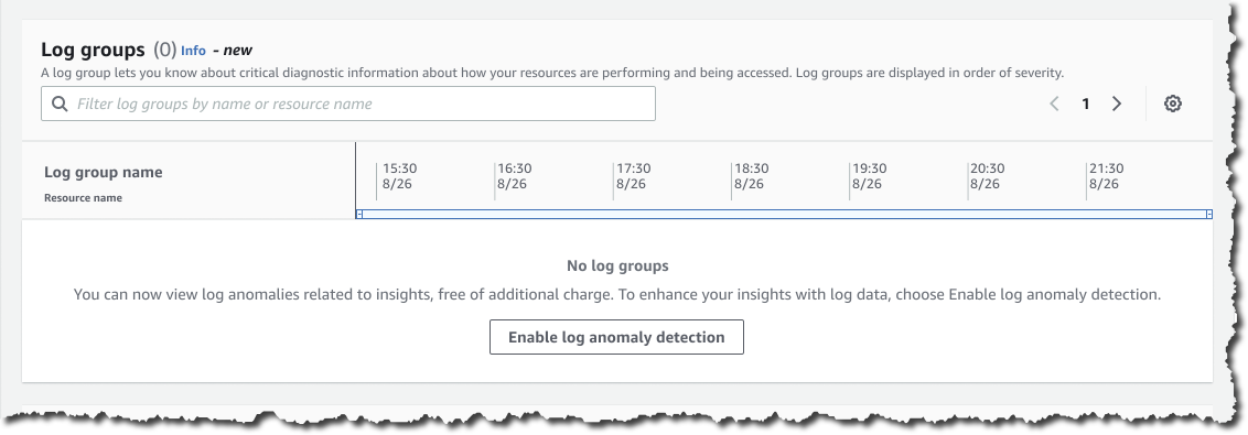
Log Anomaly Detection
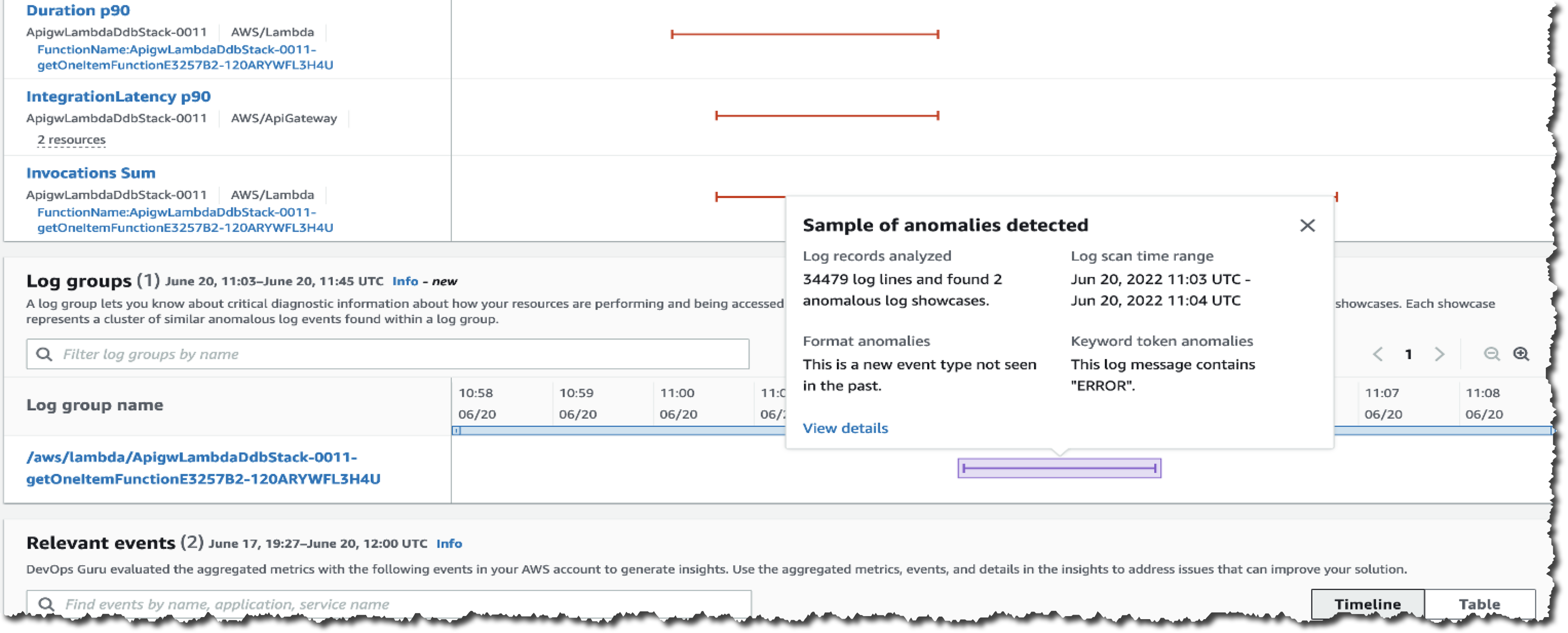
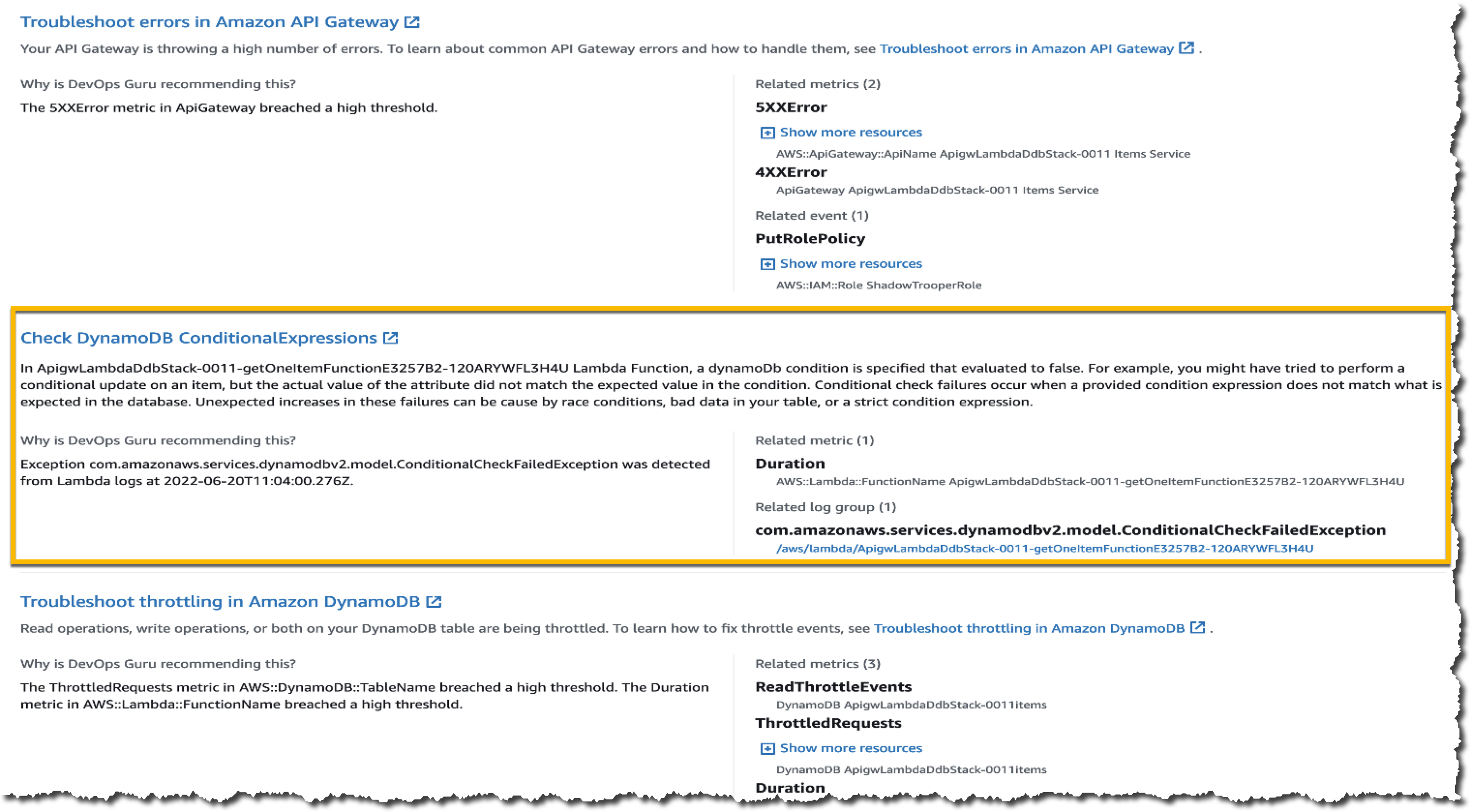
After a few hours, I can visit the DevOps Guru dashboard to check for insights. Here, I get some findings from DevOps Guru, as seen in the following screenshots:
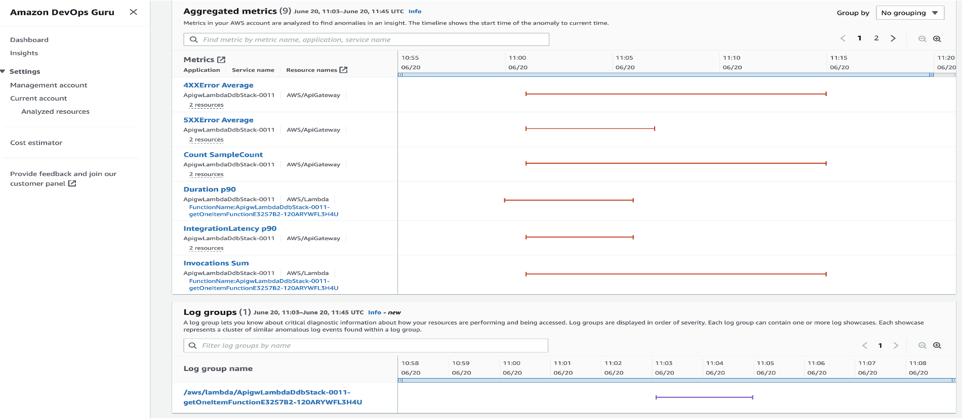
With Log Anomaly Detection, DevOps Guru will show the findings of my serverless API in the Log groups section, as seen in the following screenshot:
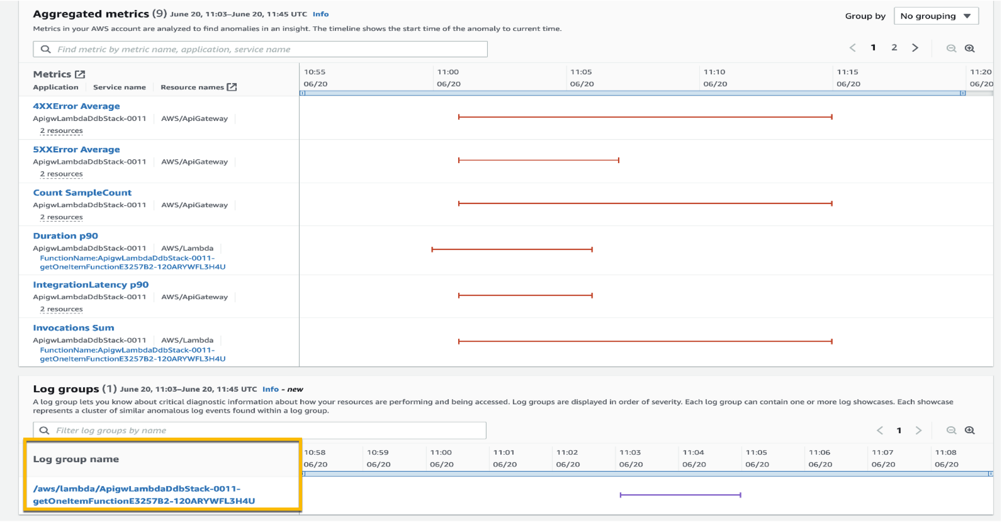
I can hover over the anomaly and get a high-level summary of the contextualized enrichment data found in this log group. It also provides me with additional information, including the number of log records analyzed and the log scan time range. From this information, I know these anomalies are new event types that have not been detected in the past with the keyword ERROR.
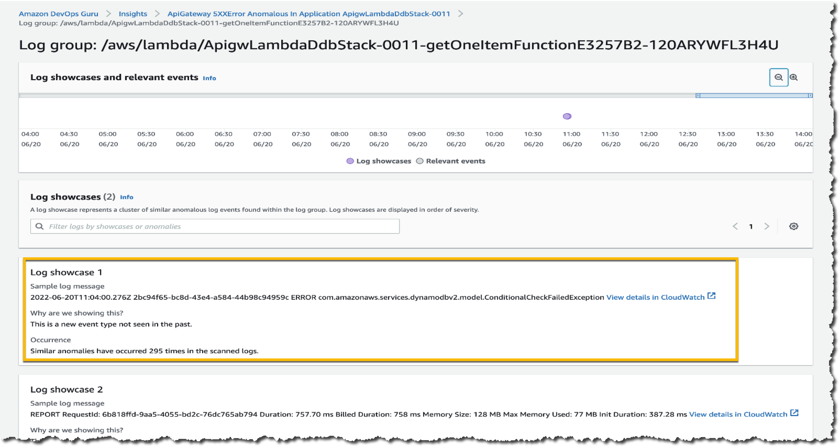
To investigate further, I can select the log group link and go to the Detail page. The graph shows relevant events that might have occurred around these log showcases, which is a helpful context for troubleshooting the root cause. This Detail page includes different showcases, each representing a cluster of similar log events, like exception keywords and numerical anomalies, found in the logs at the time of the anomaly.
Looking at the first log showcase, I noticed a ConditionalCheckFailedException error within the AWS Lambda function. This can occur when AWS Lambda fails to call DynamoDB. From here, I learned that there was an error in the conditional check section, and I reviewed the logic on AWS Lambda. I can also investigate related CloudWatch Logs groups by selecting View details in CloudWatch links.
One thing I want to emphasize here is that DevOps Guru identifies significant events related to application performance and helps me to see the important things I need to focus on by separating the signal from the noise.
Targeted Recommendations
In addition to anomaly detection of logs, this new feature also provides precise recommendations based on the findings in the logs. You can find these recommendations on the Insights page, by scrolling down to find the Recommendations section.
Here, I get some recommendations from DevOps Guru, which make it easier for me to take immediate steps to remediate the issue. One recommendation shown in the following image is Check DynamoDB ConditionalExpression, which relates to an anomaly found in the logs derived from AWS Lambda.
Availability
You can use DevOps Guru Log Anomaly Detection and Recommendations today at no additional charge in all Regions where DevOps Guru is available, US East (Ohio), US East (N. Virginia), US West (Oregon), Asia Pacific (Singapore), Asia Pacific (Sydney), Asia Pacific (Tokyo), Europe (Frankfurt), Europe (Ireland), and Europe (Stockholm).
To learn more, please visit Amazon DevOps Guru web site and technical documentation, and get started today.
Happy building
— Donnie
Post Syndicated from Harshida Patel original https://aws.amazon.com/blogs/big-data/achieve-fine-grained-data-security-with-row-level-access-control-in-amazon-redshift/
Amazon Redshift is a fully managed, petabyte-scale data warehouse service in the cloud. With Amazon Redshift, you can analyze all your data to derive holistic insights about your business and your customers. One of the challenges with security is that enterprises want to provide fine-grained access control at the row level for sensitive data. You can do this by creating views or using different databases and schemas for different users. However, this approach isn’t scalable and becomes complex to maintain over time. Customers have asked us to simplify the process of securing their data by providing the ability to control granular access.
Row-level security (RLS) in Amazon Redshift is built on the foundation of role-based access control (RBAC). RLS allows you to control which users or roles can access specific records of data within tables, based on security policies that are defined at the database object level. This new RLS capability in Amazon Redshift enables you to dynamically filter existing rows of data in a table. This is in addition to column-level access control, where you can grant users permissions to a subset of columns. Now you can combine column-level access control with RLS policies to further restrict access to particular rows of visible columns.
In this post, we explore the row-level security features of Amazon Redshift and how you can use roles to simplify managing privileges required to your end-users.
TrustLogix is a Norwest Venture Partners backed cloud security startup in the Data Security Governance space. TrustLogix delivers powerful monitoring, observability, audit, and fine-grained data entitlement capabilities that empower Amazon Redshift clients to implement data-centric security for their digital transformation initiatives.
“We’re excited about this new and deeper level of integration with Amazon Redshift. Our joint customers in security-forward and highly regulated sectors including financial services, healthcare, and pharmaceutical need to have incredibly fine-grained control over which users are allowed to access what data, and under which specific contexts. The new role-level security capabilities will allow our customers to precisely dictate data access controls based on their business entitlements while abstracting them away from the technical complexities. The new Amazon Redshift RLS capability will enable our joint customers to model policies at the business level, deploy and enforce them via a security-as-code model, ensuring secure and consistent access to their sensitive data.”
-Ganesh Kirti, founder and CEO of TrustLogix.
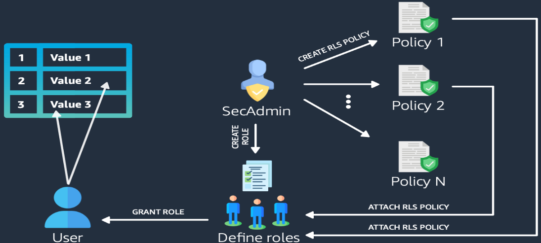
Row-level security allows you to restrict some records to certain users or roles, depending on the content of those records. With RLS, you can define policies to enforce fine-grained row-level access control. When creating RLS policies, you can specify expressions that control whether Amazon Redshift returns any existing rows in a table in a query. With RLS policies limiting access, you don’t have to add or externalize additional conditions in your queries. You can attach multiple policies to a table, and a single policy can be attached to multiple tables, making this implementation relationship many-to-many. Once attached, the RLS policy is applied on a relation and a set of users or roles, to run SELECT, UPDATE, and DELETE operations. All attached RLS policies have to evaluate together to true for a record to be returned by query. The RBAC built-in role, security admin, is responsible for managing the policies.
The following diagram illustrates the workflow.
With RLS, you can do the following:
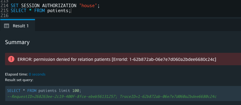
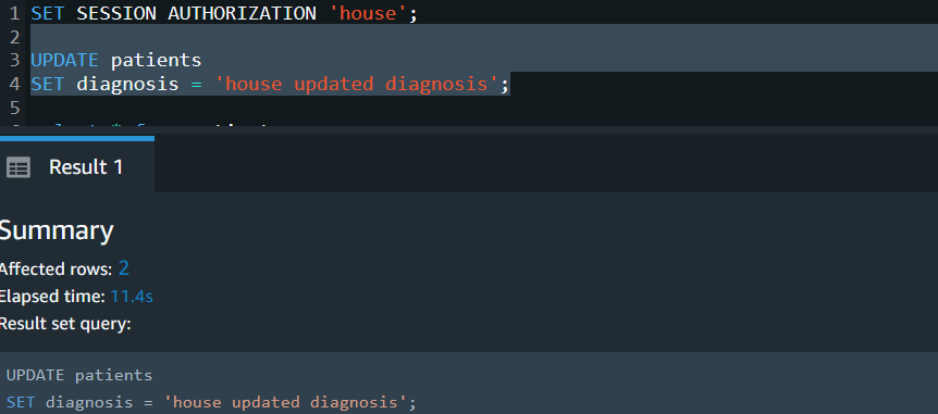
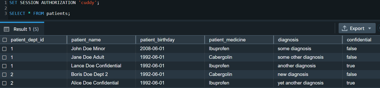
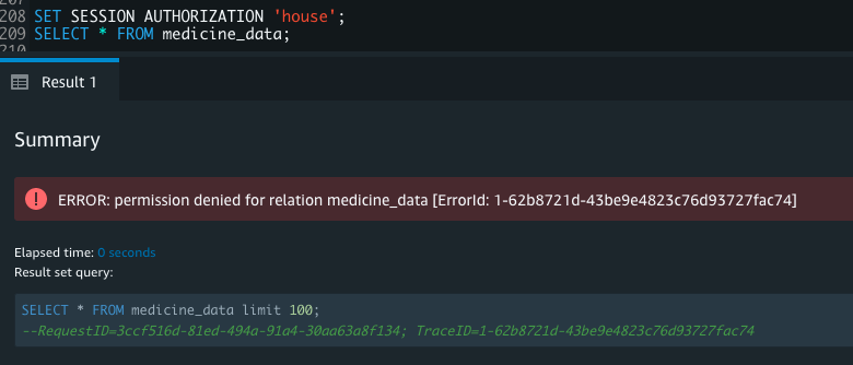
house is part of the role staff. When house queries the table, only one record pertaining to house is returned; the rest of the records are filtered as per the RLS policy. The sensitive column is also restricted, so users from the role staff can’t see this column. User cuddy is part of the role manager. When cuddy queries the employees table, all records and columns are returned.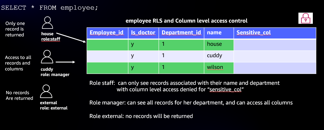
With row-level security, many use cases for fine-grained access controls become possible. The following are just some of the many application use cases:
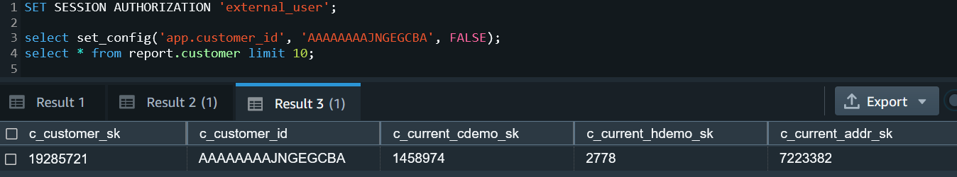
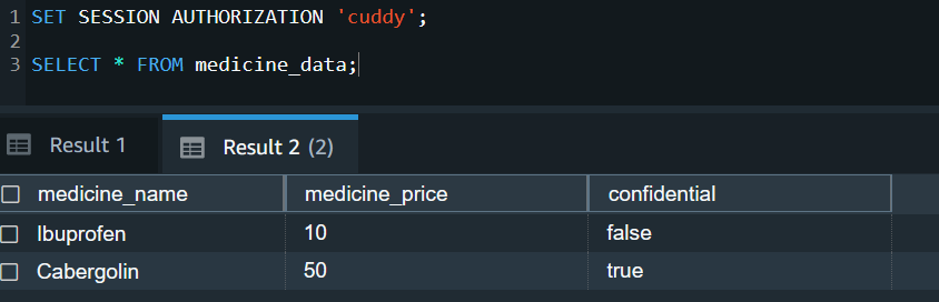
In the following example use cases, we illustrate enforcing an RLS policy on a fictitious healthcare setup. We demonstrate RLS on the medicine_data table and patients table, based on a policy established for managers, doctors, and departments. We also cover using a custom session variable context to set an RLS policy for the multi-tenant table customer.
To download the script and set up the tables, choose rls_createtable.sql.
To grant read and write access, complete the following steps:
secadmin role:
STAFF, MANAGER, and EXTERNAL:
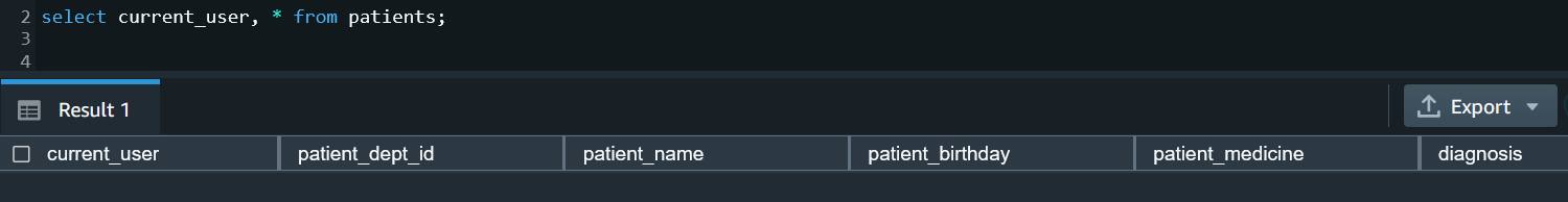
MANAGER can access all columns in the Patients and Medicine_data tables, including the confidential column that defines RLS policies:
STAFF role can access all columns except the confidential column:
We can see RLS in action with a SELECT query:
As a super user and secadmin, you can query the svv_rls_applied_policy to audit and monitor the policies applied. We discuss system views for auditing and monitoring more later in this post.
Post Syndicated from Danilo Poccia original https://aws.amazon.com/blogs/aws/amazon-redshift-serverless-now-generally-available-with-new-capabilities/
Last year at re:Invent, we introduced the preview of Amazon Redshift Serverless, a serverless option of Amazon Redshift that lets you analyze data at any scale without having to manage data warehouse infrastructure. You just need to load and query your data, and you pay only for what you use. This allows more companies to build a modern data strategy, especially for use cases where analytics workloads are not running 24-7 and the data warehouse is not active all the time. It is also applicable to companies where the use of data expands within the organization and users in new departments want to run analytics without having to take ownership of data warehouse infrastructure.
Today, I am happy to share that Amazon Redshift Serverless is generally available and that we added many new capabilities. We are also reducing Amazon Redshift Serverless compute costs compared to the preview.
You can now create multiple serverless endpoints per AWS account and Region using namespaces and workgroups:
Each namespace can have only one workgroup associated with it. Conversely, each workgroup can be associated with only one namespace. You can have a namespace without any workgroup associated with it, for example, to use it only for sharing data with other namespaces in the same or another AWS account or Region.
In your workgroup configuration, you can now use query monitoring rules to help keep your costs under control. Also, the way Amazon Redshift Serverless automatically scales data warehouse capacity is more intelligent to deliver fast performance for demanding and unpredictable workloads.
Let’s see how this works with a quick demo. Then, I’ll show you what you can do with namespaces and workgroups.
Using Amazon Redshift Serverless
In the Amazon Redshift console, I select Redshift serverless in the navigation pane. To get started, I choose Use default settings to configure a namespace and a workgroup with the most common options. For example, I’ll be able to connect using my default VPC and default security group.

With the default settings, the only option left to configure is Permissions. Here, I can specify how Amazon Redshift can interact with other services such as S3, Amazon CloudWatch Logs, Amazon SageMaker, and AWS Glue. To load data later, I give Amazon Redshift access to an S3 bucket. I choose Manage IAM roles and then Create IAM role.
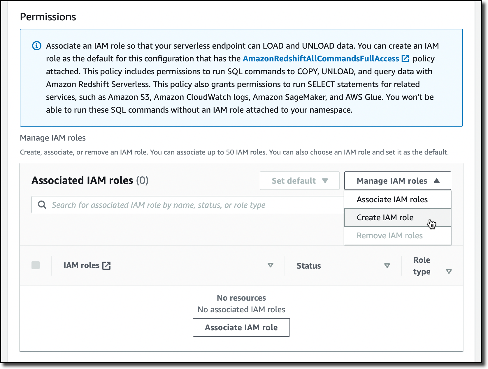
When creating the IAM role, I select the option to give access to specific S3 buckets and pick an S3 bucket in the same AWS Region. Then, I choose Create IAM role as default to complete the creation of the role and to automatically use it as the default role for the namespace.

I choose Save configuration and after a few minutes the database is ready for use. In the Serverless dashboard, I choose Query data to open the Redshift query editor v2. There, I follow the instructions in the Amazon Redshift Database Developer guide to load a sample database. If you want to do a quick test, a few sample databases (including the one I am using here) are already available in the sample_data_dev database. Note also that loading data into Amazon Redshift is not required for running queries. I can use data from an S3 data lake in my queries by creating an external schema and an external table.
The sample database consists of seven tables and tracks sales activity for a fictional “TICKIT” website, where users buy and sell tickets for sporting events, shows, and concerts.
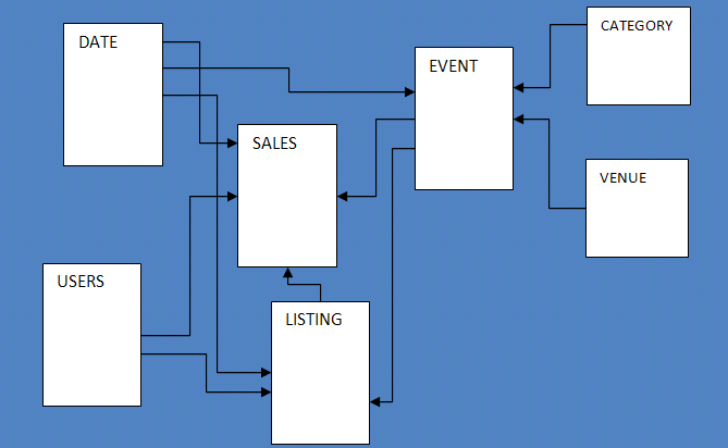
To configure the database schema, I run a few SQL commands to create the users, venue, category, date, event, listing, and sales tables.

Then, I download the tickitdb.zip file that contains the sample data for the database tables. I unzip and load the files to a tickit folder in the same S3 bucket I used when configuring the IAM role.
Now, I can use the COPY command to load the data from the S3 bucket into my database. For example, to load data into the users table:
copy users from 's3://MYBUCKET/tickit/allusers_pipe.txt' iam_role default;
The file containing the data for the sales table uses tab-separated values:
copy sales from 's3://MYBUCKET/tickit/sales_tab.txt' iam_role default delimiter '\t' timeformat 'MM/DD/YYYY HH:MI:SS';After I load data in all tables, I start running some queries. For example, the following query joins five tables to find the top five sellers for events based in California (note that the sample data is for the year 2008):
select sellerid, username, (firstname ||' '|| lastname) as sellername, venuestate, sum(qtysold)
from sales, date, users, event, venue
where sales.sellerid = users.userid
and sales.dateid = date.dateid
and sales.eventid = event.eventid
and event.venueid = venue.venueid
and year = 2008
and venuestate = 'CA'
group by sellerid, username, sellername, venuestate
order by 5 desc
limit 5;
Now that my database is ready, let’s see what I can do by configuring Amazon Redshift Serverless namespaces and workgroups.
Using and Configuring Namespaces
Namespaces are collections of database data and their security configurations. In the navigation pane of the Amazon Redshift console, I choose Namespace configuration. In the list, I choose the default namespace that I just created.
In the Data backup tab, I can create or restore a snapshot or restore data from one of the recovery points that are automatically created every 30 minutes and kept for 24 hours. That can be useful to recover data in case of accidental writes or deletes.

In the Security and encryption tab, I can update permissions and encryption settings, including the AWS Key Management Service (AWS KMS) key used to encrypt and decrypt my resources. In this tab, I can also enable audit logging and export the user, connection, and user activity logs.

In the Datashares tab, I can create a datashare to share data with other namespaces and AWS accounts in the same or different Regions. In this tab, I can also create a database from a share I receive from other namespaces or AWS accounts, and I can see the subscriptions for datashares managed by AWS Data Exchange.

When I create a datashare, I can select which objects to include. For example, here I want to share only the date and event tables because they don’t contain sensitive data.

Using and Configuring Workgroups
Workgroups are collections of compute resources and their network and security settings. They provide the serverless endpoint for the namespace they are configured for. In the navigation pane of the Amazon Redshift console, I choose Workgroup configuration. In the list, I choose the default namespace that I just created.
In the Data access tab, I can update the network and security settings (for example, change the VPC, the subnets, or the security group) or make the endpoint publicly accessible. In this tab, I can also enable Enhanced VPC routing to route network traffic between my serverless database and the data repositories I use (for example, the S3 buckets used to load or unload data) through a VPC instead of the internet. To access serverless endpoints that are in another VPC or subnet, I can create a VPC endpoint managed by Amazon Redshift.

In the Limits tab, I can configure the base capacity (expressed in Redshift processing units, or RPUs) used to process my queries. Amazon Redshift Serverless scales the capacity to deal with a higher number of users. Here I also have the option to increase the base capacity to speed up my queries or decrease it to reduce costs.
In this tab, I can also set Usage limits to configure daily, weekly, and monthly thresholds to keep my costs predictable. For example, I configured a daily limit of 200 RPU-hours, and a monthly limit of 2,000 RPU-hours for my compute resources. To control the data-transfer costs for cross-Region datashares, I configured a daily limit of 3 TB and a weekly limit of 10 TB. Finally, to limit the resources used by each query, I use Query limits to time out queries running for more than 60 seconds.

Availability and Pricing
Amazon Redshift Serverless is generally available today in the US East (Ohio), US East (N. Virginia), US East (Oregon), Europe (Frankfurt), Europe (Ireland), Europe (London), Europe (Stockholm), and Asia Pacific (Seoul), Asia Pacific (Singapore), Asia Pacific (Sydney), and Asia Pacific (Tokyo) AWS Regions.
You can connect to a workgroup endpoint using your favorite client tools via JDBC/ODBC or with the Amazon Redshift query editor v2, a web-based SQL client application available on the Amazon Redshift console. When using web services-based applications (such as AWS Lambda functions or Amazon SageMaker notebooks), you can access your database and perform queries using the built-in Amazon Redshift Data API.
With Amazon Redshift Serverless, you pay only for the compute capacity your database consumes when active. The compute capacity scales up or down automatically based on your workload and shuts down during periods of inactivity to save time and costs. Your data is stored in managed storage, and you pay a GB-month rate.
To give you improved price performance and the flexibility to use Amazon Redshift Serverless for an even broader set of use cases, we are lowering the price from $0.5 to $0.375 per RPU-hour for the US East (N. Virginia) Region. Similarly, we are lowering the price in other Regions by an average of 25 percent from the preview price. For more information, see the Amazon Redshift pricing page.
To help you get practice with your own use cases, we are also providing $300 in AWS credits for 90 days to try Amazon Redshift Serverless. These credits are used to cover your costs for compute, storage, and snapshot usage of Amazon Redshift Serverless only.
Get insights from your data in seconds with Amazon Redshift Serverless.
— Danilo
Post Syndicated from original https://lwn.net/Articles/900886/
Matthew Garrett grumbles about an
apparent Microsoft policy change making it harder to boot Linux on some
systems.
So, to have Microsoft, the self-appointed steward of the UEFI
Secure Boot ecosystem, turn round and say that a bunch of binaries
that have been reviewed through processes developed in negotiation
with Microsoft, implementing technologies designed to make
management of revocation easier for Microsoft, and incorporating
fixes for vulnerabilities discovered by the developers of those
binaries who notified Microsoft of these issues despite having no
obligation to do so, and which have then been signed by Microsoft
are now considered by Microsoft to be insecure is, uh, kind of
impolite?
Post Syndicated from Sébastien Stormacq original https://aws.amazon.com/blogs/aws/new-cloud-wan-a-managed-wan-service/
I am pleased to announce the availability of AWS Cloud WAN, a new network service that makes it easy to build and operate wide area networks (WAN) that connect your data centers and branch offices, as well as multiple VPCs in multiple AWS Regions.
Typically, large enterprises have resources running in different on-premises data centers, branch offices, and in the cloud. To connect these resources, network teams build and manage their own global networks using multiple networking, security, and internet services from multiple providers. They most probably use several technologies and providers to manage cloud-based networks, to connect their data centers to the AWS cloud, and for the connectivity between on-premises data centers and branch offices. All of these networks take different approaches to connectivity, security, and monitoring, resulting in an intricate patchwork of individual networks that are complicated to configure, secure, and manage.
For example, to prevent unauthorized access to resources running across locations that are connected with different network technologies, network operation teams must piece together different firewall solutions from different vendors and then manually configure and manage the policies between them. Every new location, network appliance, and security requirement exponentially increases complexity.
With Cloud WAN, networking teams connect to AWS through their choice of local network providers, then use a central dashboard and network policies to create a unified network that connects their locations and network types. This eliminates the need to configure and manage different networks individually, even when they are based on different technologies. Cloud WAN generates a complete view of your on-premises and AWS networks to help you visualize the health, security, and performance of your entire network.
Cloud WAN provides advanced security and network isolation, and I am excited by the possibilities offered by this network segmentation. You can use policies in Cloud WAN to easily segment your network traffic regardless of how many AWS Regions or on-premises locations you add to your network. For example, you can easily isolate network traffic from retail payment processing from other traffic on your corporate network while still giving both segments access to shared corporate resources. Another example would be the isolation of your development and production environment by creating logical network segments for each environment. This makes it easier to ensure consistent security policies when connecting large numbers of locations with your VPCs especially when your policies need to apply to large groups with unique security and routing requirements. Cloud WAN maintains a consistent configuration across Regions on your behalf. In a traditional network, a segment is like a globally consistent virtual routing and forwarding (VRF) table or a layer 3 IP VPN over an MPLS network. Segments are optional; smaller organizations may use Cloud WAN with one single network segment, encompassing all your traffic.
In addition to network segmentation and the simplicity it brings to your network management tasks, I see four principal benefits of using Cloud WAN:
Centralized management and network monitoring dashboard – Network Manager provides a central dashboard for connecting and managing your branch offices, data centers, VPN connections, and Software-Defined WAN (SD-WAN), as well as your Amazon VPC and AWS Transit Gateway. This dashboard helps you monitor and view the health of your network in one place, simplifying day-to-day operations.
Centralized policy management – You define access controls and traffic routing rules in a central network policy document, expressed in JSON. When you update a policy, Cloud WAN uses a two-step process to ensure accidental errors do not affect your global network. First, you review and validate that your changes will work as expected in production. Once you approve the changes, Cloud WAN handles the configuration details for the entire network. You can change your policy document using the AWS Management Console or Cloud WAN APIs.
Multi-Region VPC connectivity – Cloud WAN connects your VPCs across AWS Regions. Using a simple network policy document, you can create global networks that connect all of your EC2 resources, or you can choose to segment them across Regions.
Built-in automation. Cloud WAN can automatically attach new VPCs and network connections to your network, so you do not need to approve each change manually. It reduces the operational overhead involved in managing a growing network. You do this by tagging attachments and defining network policies that automatically map attachments with a certain tag to a specific network segment. With this tagging structure in place, you can choose which attachments can join a segment automatically, which segments require manual approval, and if attachments on the same segment can talk to each other, all based on the tags you choose.
Let’s get started
To get started with Cloud WAN, I open the AWS Management Console. In the VPC section, there is a new entry for AWS Cloud WAN on the menu on the left. Creating and configuring a global network is a four-step process.
First, I start by creating a global network and a core network.
 After entering the Name and an optional Description, I select Next.
 After giving the core network a Name and a Description, I enter my ASN range and the list of Edge locations, and I enter a Segment name and Segment description for my default segment. The default segment is automatically enabled in all selected edge locations.
Second, I define and attach my core networking policy. The core policy defines the rule to control network access across segments and AWS Regions. Third, I configure segments and segment actions. I can see all routes and filter by network Segment and Edge location.
 And finally, I register the existing Transit Gateway to the new global network.
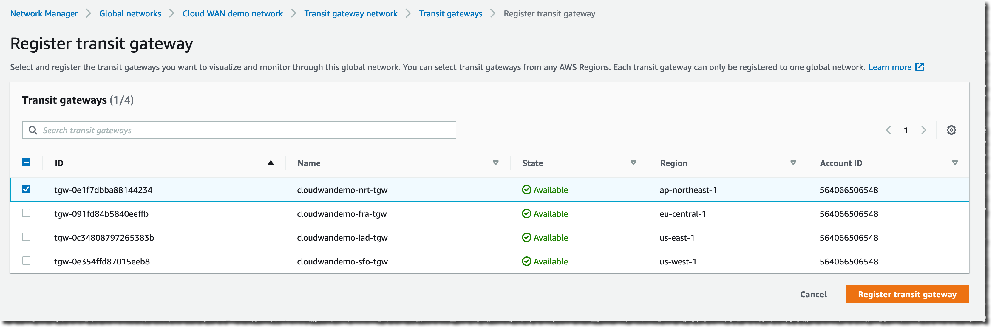
Once configured, you have a single monitoring dashboard for your global network. You have access to the network inventory.
 Or you can have more granular and detailed views with Topology graph and Topology tree.

Other considerations
During the preview period we ran for Cloud WAN, we often received the question: “When should I build networks with Cloud WAN versus Transit Gateway?” This is a valid question because both Transit Gateway and Cloud WAN allow centralized connectivity between Amazon VPC and on-premises locations. Transit Gateway is a Regional network connectivity hub and is optimal when you operate in a few AWS Regions or when you want to manage your own peering and routing configuration or prefer to use your own automation.
On the other side, Cloud WAN is a managed wide area network (WAN) that unifies your data center, branches, and AWS networks. While you can create your own global network by interconnecting multiple Transit Gateways across Regions, Cloud WAN provides built-in automation, segmentation, and configuration management features designed specifically for building and operating global networks. Cloud WAN has added features such as automated VPC attachments, integrated performance monitoring, and centralized configuration.
But the world is better together, you can peer your Transit Gateways with Cloud WAN’s Core Network Edges (CNEs) and benefit from the central management and monitoring capabilities I described earlier. The peering between Cloud WAN and Transit Gateway keeps your options open – you can migrate from one to another, or use Cloud WAN to centrally connect all your existing Transit Gateways.
But then, AWS released SiteLink in December last year. When should you use SiteLink, and when should you use AWS Cloud WAN? Depending on your use case, you might choose one, the other, or both. Cloud WAN can create and manage networks of VPCs across multiple Regions. SiteLink, on the other hand, connects Direct Connect locations together, bypassing AWS Regions to improve performance. Direct Connect is one of the several connectivity options that you will be able to natively use with Cloud WAN in the future. As of today, you interconnect Direct Connect with Cloud WAN via Transit Gateway peering connections.
Availability and Pricing
Cloud WAN is available today in US East (N. Virginia), US East (Ohio), US West (N. California), US West (Oregon), Africa (Cape Town), Asia Pacific (Mumbai), Asia Pacific (Singapore), Asia Pacific (Sydney), Asia Pacific (Tokyo), Canada (Central), Europe (Frankfurt), Europe (Ireland), Europe (London), Europe (Milan), Europe (Paris), Europe (Stockholm), and Middle East (Bahrain) AWS Regions.
As usual, there are no setup or upfront fees, and billing is on-demand based on your actual usage. There are four factors that determine what you pay for using AWS Cloud WAN. First, the number of Core Network Edges (CNEs) deployed. Second, the number of attachments to each CNE. An attachment might be an Amazon VPC, a VPN, or an SD-WAN. Third, the number of Transit Gateways peered with your CNEs. And fourth, there is a data processing charge for traffic sent through each CNE.
On top of these factors that are specific to Cloud WAN, sending data between Regions triggers an EC2 inter-Region data transfer out charge. While EC2 inter-Region data transfer out is billed separately from Cloud WAN, it’s a factor in the total cost of the Cloud WAN service. The pricing page has the details.
Post Syndicated from Jesse Mack original https://blog.rapid7.com/2022/07/12/3-key-challenges-for-cloud-identity-and-access-management/

Identity and access management (IAM) is one of the most critical tools for today’s cloud-centric environment. Businesses’ IT architectures have become more highly distributed than ever, and users need to access a growing suite of cloud services on demand. Determining the identities of users and resources, and what services each user needs access to, is critical to cloud-native security. It provides the basis for enforcing the principle of least privilege, which aims to minimize risk by giving each user the lowest level of access they need without limiting their job effectiveness or reducing productivity.
But getting an IAM solution up and running comes with its own headaches and stresses — especially in the context of complex cloud environments. Here are three of the main challenges that security teams face when implementing a cloud IAM solution, as well as some strategies to help tackle them.
The first step is always the hardest, right? Getting your entire team onboarded with the correct level of access is the earliest snag many organizations hit with IAM.
Obviously, large enterprises with huge numbers of employees will likely feel this pinch more than others. But with cloud complexity now fully entrenched at even small and mid-sized organizations, making sure each team member has the correct level of access to the right applications on day one can seem like an overwhelming task, no matter how large your team. The stakes of a misstep here are high: Improperly configuring user access not only introduces risk, it can also slow down employees in their critical tasks — hindering the business’s ability to provide value for customers.
One of the keys to success here is having a tool that makes it easy to adhere to the principle of least-privileged access. Role-based access controls, for example, help assign user rights in an automated way based on the team member’s job function and department. This can help take some pressure off the security team to stay up-to-the-minute on every employee’s access and allows necessary changes to be made faster.
Cloud adoption is big and sprawling. The average company now uses 110 software-as-a-service (SaaS) applications, and for large enterprises, some estimates put the number of cloud services in play at over 1,900.
That’s a whole lot of solutions to integrate with your IAM platform — and if every user currently has a separate, distinct identity when they sign on to each application, the numbers grow exponentially. When implementing IAM, network administrators need to take full stock of all cloud services in play, as well as ensure any new services that teams subsequently bring on board are integrated with IAM. At large, growing companies where things move quickly, that can mean provisioning several new services per week or per month.
To help alleviate these issues and reduce complexity, it’s critical to integrate your IAM platform with a single sign-on (SSO) tool that allows users to access SaaS applications with a single identity, linked to a central directory. While there are still quite a number of integrations necessary to make this happen, the one-two punch of IAM and SSO provides much-needed structure to that complex picture. It also helps out the end user, providing them the convenience of only needing one sign-on identity to access all their critical applications.
In cloud computing as in life, change is the only constant. Not only are organizations onboarding new cloud services all the time, but they also see employees leave, change roles, switch offices, and transition to fully remote work. Any of these actions may bring about some needed adjustment in a team member’s access permissions.
IAM can’t be a set-it-and-forget-it solution. Improperly provisioning and deprovisioning users — i.e., granting access where it may not be needed, or failing to remove access when an employee leaves or switches teams — can lead to major gaps in an organization’s risk profile. It can allow the proliferation of so-called “zombie accounts,” identities that still exist for users who are inactive. It can also result in an excess of admin accounts, giving users the highest level of access even if they may not need it.
Automation is one of the best tools to help security teams circumvent issues associated with out-of-date identities and improper access provisioning. If you have rules set up for reducing or removing access privileges when an employee leaves, for example, you can get ahead of the problem before it grows. Behavioral analytics can also be immensely helpful in spotting dormant accounts or removing access to applications and services that haven’t been used for a prolonged period of time. It can also help identify unusual user actions, which could indicate an account has been provisioned incorrectly.
Complexity is the tradeoff of the flexibility and scale that cloud architectures offer — which makes it all the more important to streamline wherever possible. Having a unified solution that provides IAM alongside the other key elements of cloud security can save security teams a lot of time and stress, helping them identify and remediate risks more quickly.
What kinds of IAM challenges is your team facing? Come chat with us at AWS re:Inforce on July 26-27, 2022 — we want to hear how you’re tackling IAM as you work toward fully cloud-native security.
Additional reading:
Post Syndicated from original https://lwn.net/Articles/900855/
Security updates have been issued by Debian (chromium), Mageia (openssl and webkit2), Slackware (seamonkey), SUSE (crash, curl, freerdp, ignition, libnbd, and python3), and Ubuntu (dovecot and python-ldap).
Post Syndicated from Laura Schilder original https://blog.zabbix.com/keep-things-cool-with-zabbix/21534/
Do your friends, colleagues or maybe even your significant other have a nasty habit of leaving the fridge half-open causing you a frustrating evening and potentially even ruining your cherished batch of pistachio-flavored ice cream?
With the right thermometer and a little Zabbix knowledge, you can configure Zabbix to keep a watchful eye on the temperature of your fridge and alert you whenever things in your fridge are about to stop being cool.
The Internet of things represents objects that are capable of autonomously transferring data over a network. The objects can be something like a temperature sensor, a smart fridge, or an electric scooter Even a garbage can and a vending equipped with proper sensors can be IoT objects.
Well, let’s go back to the thermometer that I was talking about. That thermometer is also an IoT device and it uses a specific protocol; for this specific one, we will use an aggregator: The Things Network (TTN).
But why do we need an aggregator? If you plan on monitoring a large number of sensors you will have to establish connections to each of these sensors individually. An aggregator can be used as the central point of communication, instead of directly connecting to each of the sensors.
In this blog post we will be using the following components:
Now, not just any thermometer can connect to the internet. But the thermometer I used is one from The Things Network. The Things Network is open source, just like Zabbix, and works with LoRaWAN. If you do not know what LoRaWAN is just keep reading and I will explain what it is.
LoRaWAN stands for Long Range Wide Area Network and it’s a protocol that is made for long-distance communication and low power consumption. Certain nodes use this protocol and send information via radio. For Europe the frequency used for transferring data is 868MHz. This is how the thermometer sends the temperature to The Things Network.
Before we are able to see the sent values, we do have to configure a gateway and add it to The Things Network. After adding a gateway to TTN, the only thing remaining is having to add the thermometers. All of this information is also available in The Things Network console. We’re going to set up an MQTT connection via The Things Network console, and configure it so Zabbix can collect, process, and visualize your IoT data, as well as receive alerts whenever the temperature in our fridge gets too hot or too cold.
What is MQTT? In short – MQTT is a lightweight network protocol. MQTT is designed for remote locations that have devices with resources that have limited bandwidth. It has to run over a transport protocol and is characterized by: Ordered, lossless and bi-directional connections. Typically, TCP/IP connections are used for this. It also is an OASIS standard and an ISO recommendation.
Let’s start by adding a gateway to The Things Network. To do that, you will have to create an account on the things stack and own a gateway. But, before we get started, check what kind of gateway you have. We will be using the gateway that is meant to be inside a building. If that is done let’s start with adding it to TTN.
Let’s start at the beginning. Open the TTN webpage and log in. Easy as that. Now when you see this screen: click on the Go to gateways button.
After that, you click on the white Claim gateway button. Do not confuse it with the Add gateway button – we need to press Claim gateway.
All the fields you see on the next page will have to be filled in:
As I mentioned before the frequency should be around 868MHz. For this example, I will just use the recommended frequency. After that, click on the Claim gateway button. The gateway should work after this. If you do not know what to fill in the form fields, you can find all the information you need on the backside of your gateway.
This is what it will look like when you have successfully claimed the gateway:
Since we now have a gateway we can add the thermometer to The Things Network. To do this, we have to go to the Application tab in the console. Once we clicked on the Application tab, it will be empty. We will have to make our own application before we can add the thermometer and we will do that by pressing the Add application button. Once clicked, you should see the following:
After you have created your application, click on it and you will see a screen like this:

There you will have to go to End devices and click on Add devices. It will bring you to a screen like this:

Now, you will see just one drop-down menu, but once you start filling them in, additional menus will show up. In our case, we’re using a thermometer from Dragino. After filling in the model and region, the screen should look something like this:
For step two, we had to grab the box in which the sensor was shipped. Inside the box is a sticker with all the information that you need. When you have filled in all the fields, click on the Add device button. After adding the device it will look something like this:
Now, that’s all for adding the thermometers. If everything works, we will just have to set up an MQTT connection between The Things Network and Zabbix. On the TTN side, we have to go to integrations, and then MQTT. Everything you have on that page we can just copy. Generate an API key and copy it. Save it as we will need it later.
After all these steps on The Things Network side, we will finally move to Zabbix. What we will do first in Zabbix is make sure that we can get the information from The Things Network. This will be done via MQTT. For that, we will need Zabbix agent 2. Now there are of course more steps than just that. So, let me explain.
Let’s start by downloading Zabbix agent 2 (if you already have it you can skip this step) for that we will use this command:
dnf install zabbix-agent2
Once the agent is installed, we will have to modify the config file:
vim /etc/zabbix/zabbix_agent2.conf
I am using vim, but if you want to use something else, feel free to use another text editor. Once the configuration file has been opened, we will go ahead and change the Hostname parameter. We will be changing it to this:
Hostname=TTN
Don’t forget to start (or restart, if the agent 2 has already been installed) your agent 2 service.
systemctl start zabbix-agent2
Now that we have that out of the way we can start by making a new host. It will be a regular Zabbix host. This is what mine looks like:

Note that the Host name here matches the Hostname parameter which we edited in the previous step. Do you recall when I said that you have to copy all the MQTT information from The Things Network? Well, we will use it here. We will have to make an item that will use the Zabbix agent (active) item type to get the information. Now, for the key, we can select the mqtt key from Zabbix but we will be missing some of the required parameters. The key will have to look something like this:
mqtt.get[broker,topic,username,password]
In the end, the item itself will look something like this:
In our case, the key looks like this:
mqtt.get[tls://eu1.cloud.thethings.network:8883, #, thermometers@ttn, NNSXS.EMK3T5FLBB2YPLYWXLP7BYOG7JHFSBKEUG23BMY.IJSZ4AC475CU5JJOLRJRYLDU6MXEODWCUYIOLZSAWSXP4L32473Q].
To check if it works just navigate to Monitoring – Latest data, find our host and you should see the collected data. It should look something like this:
{"v3/thermometers@ttn/devices/eui-a84041a4e10000/up":"{\"end_device_ids\":{\"device_id\":\"eui-a84041a4e1000000\",\"application_ids\":{\"application_id\":\"thermometers\"},\"dev_eui\":\"A84041A4E10000\",\"join_eui\":\"A000000000000100\",\"dev_addr\":\"260B4F08\"},\"correlation_ids\":[\"as:up:01G7CJFS1180WT7M2GHQRWVFKA\",\"gs:conn:01G7A3RFY7CT62SGBH2BGJ7T31\",\"gs:up:host:01G7A3RG2EWWCHEW9HVBQ6KA5A\",\"gs:uplink:01G7CJFRTGY0NV6R4Y8AV9XKGG\",\"ns:uplink:01G7CJFRTHSDCK3DVR7EDGJY5V\",\"rpc:/ttn.lorawan.v3.GsNs/HandleUplink:01G7CJFRTHP5JMRVSNP8ZZR1X1\",\"rpc:/ttn.lorawan.v3.NsAs/HandleUplink:01G7CJFS10A5RAD5SE864Q99R8\"],\"received_at\":\"2022-07-07T14:54:39.137181192Z\",\"uplink_message\":{\"session_key_id\":\"AYGu5fFGW+vxth9cFIw2+g==\",\"f_port\":2,\"f_cnt\":601,\"frm_payload\":\"y/kH5QIoAX//f/8=\",\"decoded_payload\":{\"BatV\":3.065,\"Bat_status\":3,\"Ext_sensor\":\"Temperature Sensor\",\"Hum_SHT\":55.2,\"TempC_DS\":327.67,\"TempC_SHT\":20.21},\"rx_metadata\":[{\"gateway_ids\":{\"gateway_id\":\"gateway7\",\"eui\":\"58A0CBFFFE803D17\"},\"time\":\"2022-07-07T14:54:38.903268098Z\",\"timestamp\":945990219,\"rssi\":-61,\"channel_rssi\":-61,\"snr\":7.5,\"uplink_token\":\"ChYKFAoIZ2F0ZXdheTcSCFigy//+gD0XEMvUisMDGgwIrueblgYQ/fHaugMg+Omki8TiEioMCK7nm5YGEIKO264D\"}],\"settings\":{\"data_rate\":{\"lora\":{\"bandwidth\":125000,\"spreading_factor\":7}},\"coding_rate\":\"4/5\",\"frequency\":\"868500000\",\"timestamp\":945990219,\"time\":\"2022-07-07T14:54:38.903268098Z\"},\"received_at\":\"2022-07-07T14:54:38.929160377Z\",\"consumed_airtime\":\"0.061696s\",\"version_ids\":{\"brand_id\":\"dragino\",\"model_id\":\"lht65\",\"hardware_version\":\"_unknown_hw_version_\",\"firmware_version\":\"1.8\",\"band_id\":\"EU_863_870\"},\"network_ids\":{\"net_id\":\"000013\",\"tenant_id\":\"ttn\",\"cluster_id\":\"eu1\",\"cluster_address\":\"eu1.cloud.thethings.network\"}}}"}
Now, after seeing all the data you want to be able to read it normally. Well, for that we will use Low-Level Discovery. It will also help add the thermometer to Zabbix.
To achieve our goal we will start by navigating to the Configuration – Hosts page. Select the host that you created earlier. Once there, select Discovery rules at the top. Now we are going to create a new Low-level discovery rule. It will be a dependent item. The master item is the item we made in the previous step. Once you have done that, it should look like so:

But we have not finished yet. We will also need to add a pre-processing step. For the pre-processing step, we need to provide a javascript script. The data that has been sent is not ‘native’ Zabbix LLD data, so we need to make it suitable for Zabbix.
We will use a script like this to format our data:
var lld = [];
var regexp = /@ttn\/devices\/([\w-]+)/g;
var lines = value.split("\n");
var lines_num = lines.length;
for (i = 0; i < lines_num; i++)
{
var match = regexp.exec(lines);
var row = {};
row["{#SENSOR}"] = match[1];
lld.push(row);
}
return JSON.stringify(lld);
In the script above we are transforming the data into a format that Zabbix can use it. Let’s drill it down line by line:
Line 1: Declare a new array with name lld
Line 2: Declare a regex with a specific value
Line 3: Let’s split the received value into an array of substrings. Splitting happens on the value “\n” which represents a newline
Line 4: Count the number of lines
Line 5: A For loop to populate the array that is declared in line 1.
Line 7: Match the regex in the lines.
Line 8: Declare an object with the name ‘row’
Line 9: Add the text {#SENSOR} with the 1st value of the variable ‘match’
Line 10: Push the row object into the lld array
Line 12: Convert the lld array into a JSON string
After Line 12, you will get something like this returned:
[{"{#SENSOR}":"eui-a84041a4exxxxxxx"},{"{#SENSOR}":"eui-a84041a4eyyyyyyy"}]
Now the data is formatted into the Zabbix LLD format, ready to be parsed.
Once the preprocessing step is added, the rule should be complete. This means that Zabbix will start discovering the thermometers, but no items are created by just adding the LLD rule like we have done so far. We also need to add the item prototypes.
I will use temperature for the internal sensor as an example here. So, let’s start at the beginning and go to Item prototypes. We will add a new item prototype. In the name and key fields, we will use the Low-level discovery macro: {#SENSOR}. The key is arbitrary – we ill put our LLD macro as a parameter, to make each item created from the prototypes unique. For units, we will use C because it stands for temperature in Celsius. When finished, it should look like this:

Now, if you look closely at the screenshot I also have a tag and preprocessing step. You can see the tag configuration in the image below. The tag will be used for filtering and providing additional information – the sensor ID.

As for the item prototype preprocessing step – it is a little bit harder. Do you remember the data that you got from the first item we made? Well, if you take that and throw in a regex, you can make the preprocessing step. What I did was go to https://regex101.com and paste the complete string we received from the master item and start matching the temperatures.
Once the regex is done, go to the Preprocessing tab in Zabbix. Add one step, and choose Regular Expression as the Name. Now the parameters will be (in case of this thermometer):
TempC_SHT\\":(\d+.\d+)}
and in the output field we will use the first capture group – \1. It should look like this:

If we take a careful look at the data provided by the Master item, there is a “decoded payload”:
decoded_payload\":{\"BatV\":3.056,\"Bat_status\":3,\"Ext_sensor\":\"Temperature Sensor\",\"Hum_SHT\":50.8,\"TempC_DS\":21.75,\"TempC_SHT\":21.95}
From that payload, we are cherry-picking the TempC_SHT value. There are more values to collect here, like battery status, voltage, humidity, etc. This highly depends on the sensors used, of course.
In the Low-Level Discovery rule, we can keep on adding more item prototypes to parse all of these metrics and let the LLD automatically create the items from the prototypes.
After adding the low-level discovery rule and the preprocessing step you will see something like this:

Now, as you can see, Multiple items have been created from our prototypes. If you look closely, you will also notice that I get two of everything. This is because the Low-Level Discovery discovered two thermometers.
Now that everything has been configured, we can finally track the temperature of our IoT thermometers. The next time somebody leaves your fridge open, you can find out in time. Cool, right? Well, that’s just one of many IoT examples that we can start to monitor – the potential for discovering and monitoring IoT devices is unlimited. If you wish to check out the template used for this example, feel free to visit our github page.
The post Keep Things Cool with Zabbix appeared first on Zabbix Blog.
Post Syndicated from Arielle Olache original https://blog.cloudflare.com/waiting-room-event-scheduling/


You’ve got big plans for your ecommerce strategy in the form of online events — seasonal sales, open registration periods, product drops, ticket sales, and more. With all the hype you’ve generated, you’ll get a lot of site traffic, and that’s a good thing! With Waiting Room Event Scheduling, you can protect your servers from being overloaded during your event while delivering a user experience that is unique to the occasion and consistent with your brand. Available now to enterprise customers with an advanced Waiting Room subscription, Event Scheduling allows you to plan changes to your waiting room’s settings and custom queueing page ahead of time, ensuring flawless execution of your online event.
We launched Waiting Room to protect our customers’ servers during traffic spikes. Waiting Room sends excess visitors to a virtual queue during traffic surges, letting visitors in dynamically as spots become available on your site. By automatically queuing traffic that exceeds your site’s capacity, Waiting Room protects your origin servers and your customer experience. Additionally, the Waiting Room’s queuing page can be customized to match the look and feel of your site so that your users never feel as though they have left your application, ensuring a seamless customer experience.
While many of our customers use Waiting Room as an always-on failsafe against potential traffic spikes, some customers use Waiting Room to manage traffic during time-boxed online events. While these events can undoubtedly result in traffic spikes that Waiting Room safeguards against, they present unique challenges for our customers.
In the lifecycle of an online event, various stages of the event generally require the settings of a waiting room to be updated. While each customer’s event requirements are unique, consider the following customer use cases. To prevent a mad rush to a landing page that could overwhelm their site ahead of an event, some customers want to queue early arrivers in the days or hours leading up to the event. During an event, some customers want to impose stricter limits on how long visitors have to browse and complete transactions to ensure that as many visitors as possible get a fair chance to partake. After an event has concluded, many customers want to offload event traffic, blocking access to the event pages while informing users that the event has ended.
For each of these scenarios, our customers want to communicate expectations to their users and customize the look and feel of their queuing page to ensure a seamless, on-brand user experience. Combine all the use cases in the example above into one timeline, and you’ve got at least three event stages that would require waiting room settings and queuing pages to be updated, all with perfect timing.
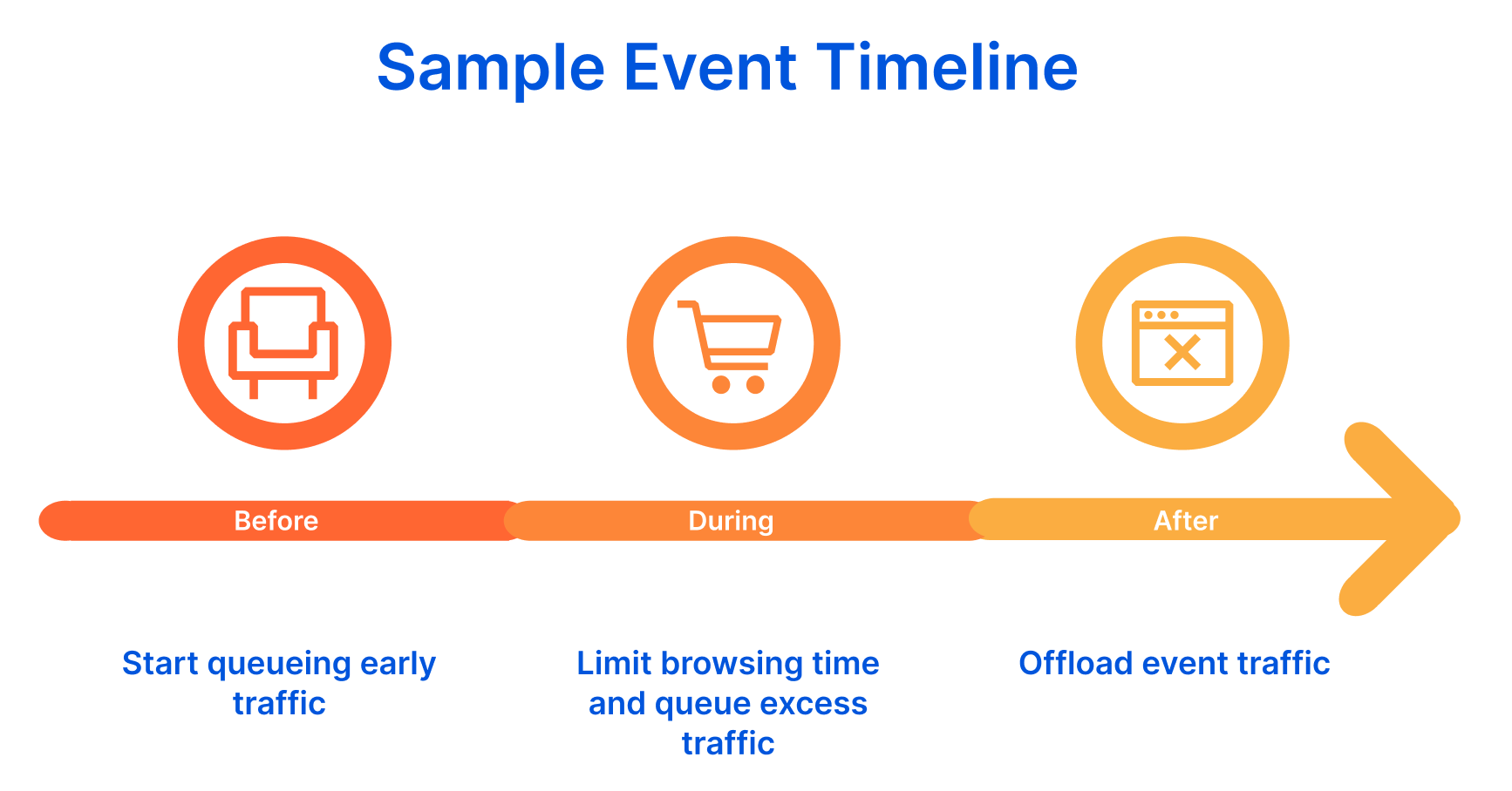
While these use cases were technically feasible with Waiting Room, they required on-the-spot updates to its configuration settings. This strategy was not ideal or practical when customers needed to be absolutely sure their waiting room would update in lockstep with the timeline of their event. In short, many customers needed to schedule changes to the behavior of their waiting room ahead of time. We built Event Scheduling to give our customers flexibility and control over when and how their waiting room settings change, ensuring that these changes will happen automatically as planned.
With Event Scheduling, you can schedule cascading changes to your waiting room ahead of time as discrete events. For each waiting room event, you can customize traffic thresholds, session duration, queuing method, and the content and styling of your queuing page. Refer to the Create Event API documentation, for a complete list of customizable event settings.
Giving our customers the ability to schedule changes to a waiting room’s settings is a game-changer for customers with event-based Waiting Room requirements, but we didn’t stop there. We’ve also added two new queueing methods — Reject and Passthrough — to give our customers more options for controlling user flow before, during and after their online events.
In the example where customers wanted to offload site traffic after an event, the Reject queuing method would do just that! A waiting room with the Reject queuing method configured will offload traffic from your site, presenting users with a static, fully customizable HTML page. Conversely, the Passthrough queuing method allows all visitors unrestricted access to your site. Unlike simply disabling your waiting room to achieve this, Passthrough has the advantage of being scheduled to turn on or off ahead of time and providing user traffic stats through the Waiting Room status endpoint.

If you prefer to have the waiting room in a completely passive state, having the waiting room on and configured with the Passthrough queueing method allows you to turn on Queue All quickly. Queue All places all new site visitors in a queue, which is a life-saver in the case of unexpected site downtime or any other crisis. Before deactivating Queue All, you can see how many users are waiting to enter your site. Queue All also overrides any active waiting room event, giving you authoritative, fast control in an emergency.
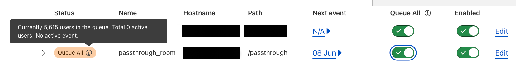
As part of an event’s configuration, you can also enable a pre-queue, a virtual holding area for visitors that arrive at your event before its start time. Pre-queues add extra protection against traffic spikes that can cause your site to crash.
To illustrate how, imagine your customer is a devoted fan trying to get tickets to their favorite band’s upcoming concert. Ticket sales open in one hour, so they visit your sales page about ten minutes before sales open. There is a static landing page on your site where the ticket sales page will be. The fan starts refreshing the page in the minutes leading up to the start time, hoping to get access as soon as sales open. Now multiply that one hopeful concert-goer by many thousands of fans, and before your sale has even begun, your site is already overwhelmed and at risk of crashing. Having a pre-queue in place protects your site from this type of user activity that has the potential to overwhelm your site at a time when stakes are very high for your brand. And with the ability to fully customize the pre-queuing page, you can still generate the same excitement you would have with your event’s landing page.
Taking it a step further, you can elect to shuffle the pre-queue, randomly assigning users who reach your application during the pre-queue period a place in line when the event starts. If your event uses the First in First Out queuing method, randomizing your pre-queue can help promote fairness, especially if your pre-queuing period spans many time zones. Like the Random queuing method, implementing a randomized pre-queue neutralizes the advantage customers in earlier time zones have to grab a place in line ahead of the event’s start time. Ultimately, fairness for your event is unique to you and your customers’ perspectives and needs. With the order of entry options available for both the pre-queue and overflow queuing during your event, you have control over managing fairness of entry to align with your unique requirements.
Similarly to configuring a waiting room, scheduling events with Waiting Room is incredibly easy and requires no coding or application changes. You will first need to have a baseline waiting room configured. Then, you can schedule events for this waiting room from the Waiting Room dashboard. In the event creation workflow, you’ll indicate when you would like the event to start and end and configure an optional pre-queue.

Unless specified otherwise, your event will always inherit the configuration settings of its associated waiting room. That way, you only need to update the waiting room settings that you would like to change for the duration of the event. You can optionally create a queuing page for your users that is unique to the event and preview what your event queuing page will look like in different queuing states and browsers, ensuring that your end-user’s experience doesn’t result in garbled CSS or broken looking pages!
Before saving your event, you will be able to review your waiting room and event settings side by side, making it easy to verify how the behavior of your waiting room will change for the duration of the event.
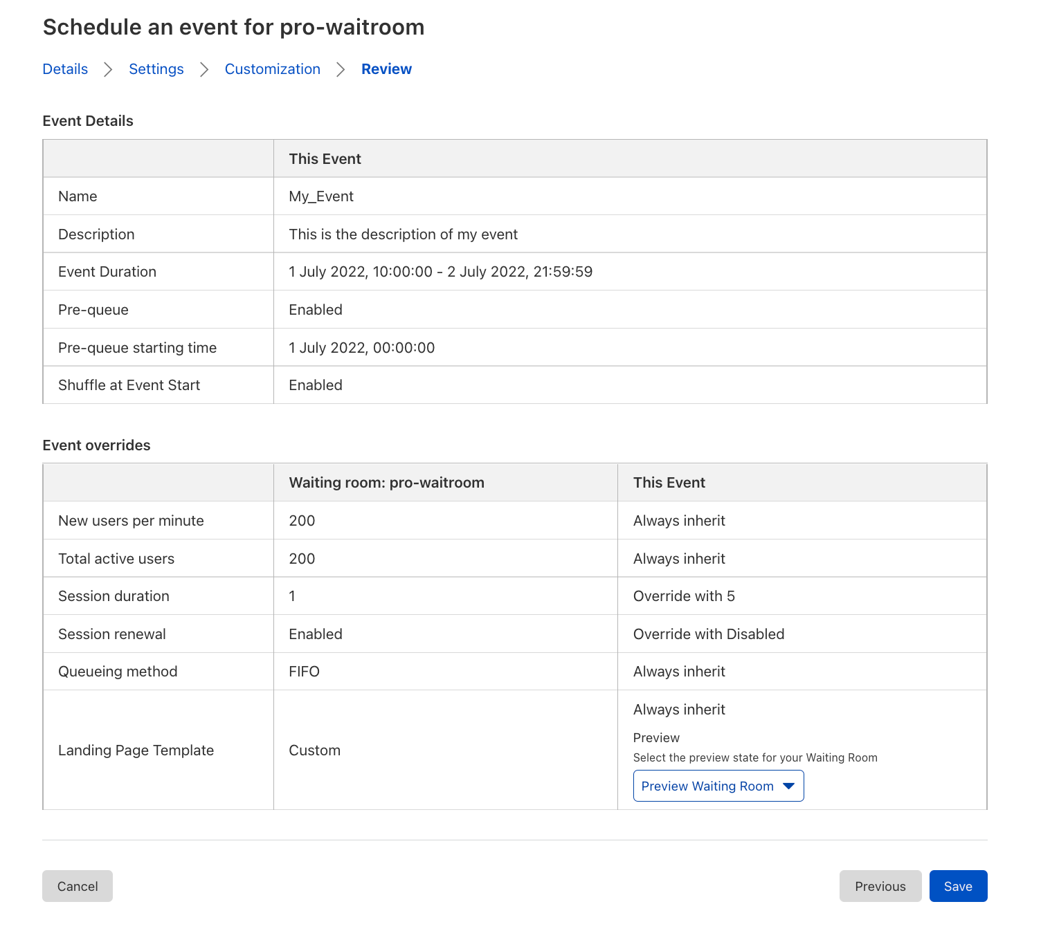
Once created, your event will appear in the Waiting Room dashboard nested under its associated waiting room. The date of each waiting room’s next event is indicated in the dashboard’s default view so that you can tell at a glance if any waiting room’s settings may change due to an upcoming event. You can expand each waiting room’s row to list upcoming events and associated durations. Additionally, if an event is live, a green dot will appear next to this date, adding extra assurance that it has kicked in.
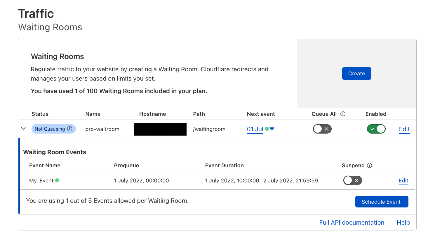
Tying it all together, let’s walk through a real-world scenario to demonstrate the versatility and practicality of Event Scheduling. In this example, we have a major women’s fashion retailer, let’s call them Shopflare, with an upcoming flash sale. A flash sale is an online sales event that is different from a regular sale in that it lasts for a brief time and offers substantial discounts or limited stock. Often, retailers target a specific audience using marketing campaigns in the days leading up to a flash sale.
In our example, Shopflare’s marketing team plans to send an email campaign to a set of target customers, promoting their Spring Flash Sale, where they will be offering free shipping and 40% off on their freshest spring arrivals for one day only! How could Shopflare use Waiting Room and Event Scheduling to help this sales event go off without a hitch?
One week before the sale, Shopflare’s web team creates a landing page with a countdown for their spring flash sale at example.com/sales/spring_flash_sale. They place a waiting room at this URL with a First In First Out queuing method and their desired traffic thresholds to allow traffic while ensuring their site remains performant. They then send an email campaign to their target audience directly linking to the sale’s landing page. With their baseline waiting room in place, early traffic to the URL will not overwhelm their site. Shopflare’s team also prepares for the upcoming sale by scheduling two cascading waiting room events ahead of time. Let’s review Shopflare’s flash sale requirements related to Waiting Room and review the steps they would take with Event Scheduling to satisfy them.
A few hours before the sale starts, Shopflare wants to allow shoppers to start “lining up” to secure a spot ahead of those who arrive after the event start time. They want to create a lottery for these early arrivers, randomly assigning them a place in line when the sale starts to mitigate the advantage that customers from earlier time zones have to secure a spot in line. To do this, they would create an event for the waiting room they have already configured.
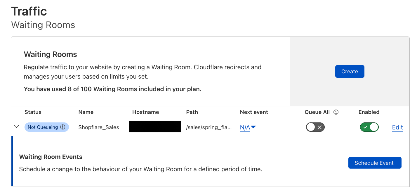
The event creation workflow consists of four main steps: Details, Settings, Customization, and Review. On the Details page of the event creation workflow, they would enter their sale start and end times, set the start time of the pre-queue and enable “Shuffle at Event Start” to create a randomized pre-queue.

While the sale is in progress, Shopflare wants an overflow queue to protect their site from being overwhelmed by traffic in excess of their waiting room limits, letting these users in First in First Out when spots open up on their site. Since their underlying waiting room is already configured with the traffic thresholds they want to enforce for the duration of the event, they would simply leave the Settings page of the event creation workflow unchanged and proceed to Customization.
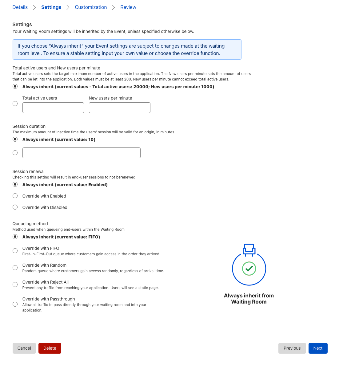
On the Customization step, Shopflare will create a custom queuing experience for their sale by uploading a custom HTML template that contains the HTML for both their pre-queueing page and their overflow queue.
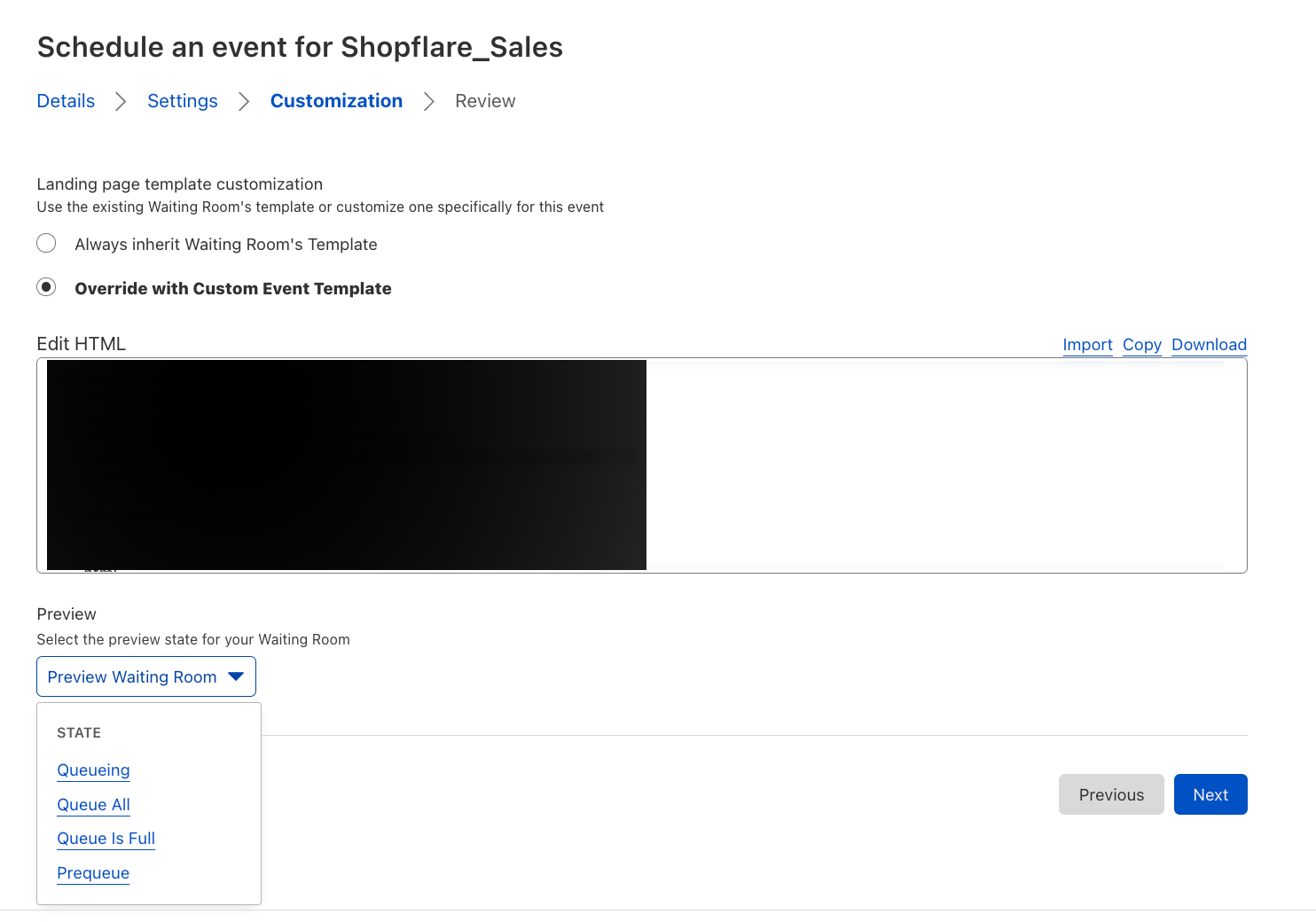
Shopflare wants their pre-queuing page to get shoppers excited about the beginning of the sale. They ensure it is branded and unique to the flash sale while setting clear expectations for shoppers. For their overflow queue, they want the same look and feel of their pre-queueing page, with updated messaging that gives shoppers an estimated wait time and explains the reason for queuing. Check out the two sample queuing pages below to see how they create a unique and informative experience for their queued customers in both the pre-queue and overflow queue.


Once the sale has ended, Shopflare wants to allow active shoppers a five-minute grace period to complete their purchases without admitting any more new visitors. For 48 hours post-sale, they would like to present all visitors with a static page letting them know the sale has concluded while providing a redirect link back to their homepage. To achieve this, Shopflare would create another event for the baseline waiting room that starts when the previous event ends without a pre-queue enabled.

To offload all new site traffic after the sale has ended while giving active shoppers a five-minute grace period, from the Settings page of the event creation workflow, they would set session duration to five minutes, disable session renewal and select the Reject All queuing method.
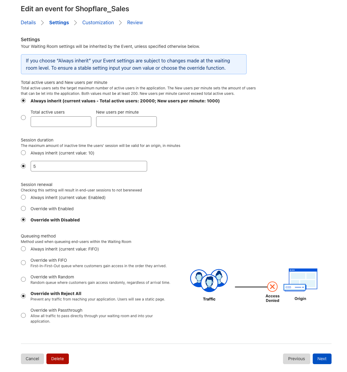
Once again, on the Customization tab, they would elect to override the underlying waiting room template with a custom event template and upload their custom Reject page HTML. They would then Review and save their event and it will appear along with their previously created event in the Waiting Room dashboard.
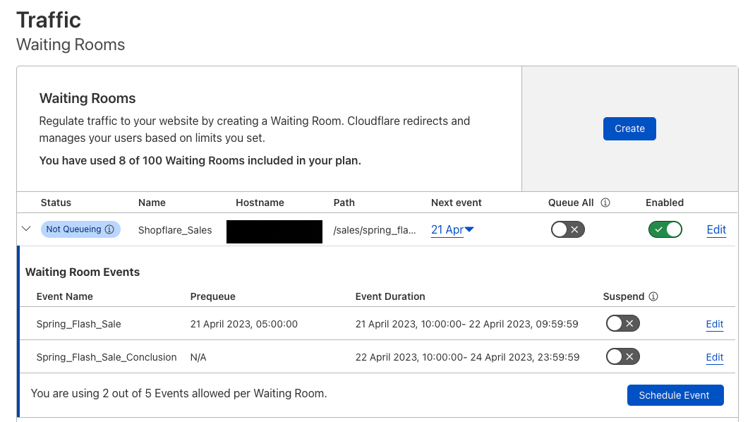
And that’s it! With their waiting room events in place, Shopflare can rest assured that their site will be protected and that their customers have an on-brand and transparent shopping experience on the big day. Each customer and online event is unique. However, you choose to manage your user traffic for your online event, Event Scheduling for Cloudflare Waiting Rooms offers the options necessary to deliver a stellar and fair user experience while protecting your application during your online event. We can’t wait to support you in your next online event!
For more on Event Scheduling and Waiting Room, check out our developer documentation.
…
We protect entire corporate networks, help customers build Internet-scale applications efficiently, accelerate any website or Internet application, ward off DDoS attacks, keep hackers at bay, and can help you on your journey to Zero Trust.
Visit 1.1.1.1 from any device to get started with our free app that makes your Internet faster and safer.To learn more about our mission to help build a better Internet, start here. If you’re looking for a new career direction, check out our open positions.
Post Syndicated from digiblurDIY original https://www.youtube.com/watch?v=NR12_B79vxU