Post Syndicated from Jeremy Ber original https://aws.amazon.com/blogs/big-data/query-your-data-streams-interactively-using-kinesis-data-analytics-studio-and-python/

Amazon Kinesis Data Analytics Studio makes it easy for customers to analyze streaming data in real time, as well as build stream processing applications powered by Apache Flink using standard SQL, Python, and Scala. Just a few clicks in the AWS Management console lets customers launch a serverless notebook to query data streams and get results in seconds. Kinesis Data Analytics reduces the complexity of building and managing Apache Flink applications. Apache Flink is an open-source framework and engine for processing data streams. It’s highly available and scalable, and it delivers high throughput and low latency for stream processing applications.

Customers running Apache Flink workloads face the non-trivial challenge of developing their distributed stream processing applications without having true visibility into the steps conducted by their application for data processing. Kinesis Data Analytics Studio combines the ease-of-use of Apache Zeppelin notebooks, with the power of the Apache Flink processing engine, to provide advanced streaming analytics capabilities in a fully-managed offering. Furthermore, it accelerates developing and running stream processing applications that continuously generate real-time insights.

In this post, we will introduce you to Kinesis Data Analytics Studio and get started querying data interactively from an Amazon Kinesis Data Stream using the Python API for Apache Flink (Pyflink). We will use a Kinesis Data Stream for this example, as it is the quickest way to begin. Kinesis Data Analytics Studio is also compatible with Amazon Managed Streaming for Apache Kafka (Amazon MSK), Amazon Simple Storage Service (Amazon S3), and various other data sources supported by Apache Flink.

Prerequisites

• Kinesis Data Stream
• Data Generator

To follow this guide and interact with your streaming data, you will need a data stream with data flowing through.

Create a Kinesis Data Stream

You can create these streams using either the Amazon Kinesis console or the following AWS Command Line Interface (AWS CLI) command. For console instructions, see Creating and Updating Data Streams in the Kinesis Data Streams Developer Guide.

To create the data stream, use the following Kinesis create-stream AWS CLI command. Your data stream will be named input-stream.

$ aws kinesis create-stream \
--stream-name input-stream \
--shard-count 1 \
--region us-east-1

Creating a Kinesis Data Analytics Studio notebook

You can start interacting with your data stream by following these steps:

1. Open the AWS Management Console and navigate to Amazon Kinesis Data Analytics for Apache Flink
2. Select the Studio tab on the main page, and select Create Studio Notebook.
3. Enter the name of your Studio notebook, and let Kinesis Data Analytics Studio create an AWS Identity and Access Management (IAM) role for this. You can create a custom role for specific use cases using the IAM Console.
4. Choose an AWS Glue Database to store the metadata around your sources and destinations used by Kinesis Data Analytics Studio.
5. Select Create Studio Notebook.

We will keep the default settings for the application, and we can scale up as needed.

Once the application has been created, select Start to start the Apache Flink application. This will take a few minutes to complete, at which point you can Open in Apache Zeppelin.

Write Sample Records to the Data Stream

In this section, you can create a Python script within the Apache Zeppelin notebook to write sample records to the stream for the application to process.

Select Create a new note in Apache Zeppelin, and name the new notebook stock-producer with the following contents:

%ipyflink
import datetime
import json
import random
import boto3

STREAM_NAME = "input-stream"
REGION = "us-east-1"


def get_data():
    return {
        'event_time': datetime.datetime.now().isoformat(),
        'ticker': random.choice(["BTC","ETH","BNB", "XRP", "DOGE"]),
        'price': round(random.random() * 100, 2)}


def generate(stream_name, kinesis_client):
    while True:
        data = get_data()
        print(data)
        kinesis_client.put_record(
            StreamName=stream_name,
            Data=json.dumps(data),
            PartitionKey="partitionkey")


if __name__ == '__main__':
    generate(STREAM_NAME, boto3.client('kinesis', region_name=REGION))

You can run the stock-producer paragraph to begin publishing messages to your Kinesis Data Stream either by pressing SHIFT + ENTER on the paragraph, or by selecting the Play button in the top-right of the paragraph.

Feel free to close or navigate away from this notebook for now, as it will continue publishing events indefinitely.

Note that this will continue publishing events until the notebook is paused or the Apache Flink cluster is shut down.

Example Applications

Apache Zeppelin supports the Apache Flink interpreter and allows for the direct use of Apache Flink within a notebook for interactive data analysis. Within the Flink Interpreter, three languages are supported at this time—Scala, Python (PyFlink), and SQL. The notebook requires a specification to one of these languages at the top of each paragraph to interpret the language properly.

%flink          - Scala environment 
%flink.pyflink  - Python Environment
%flink.ipyflink - ipython Environment
%flink.ssql     - Streaming SQL Environment
%flink.bsql     - Batch SQL Environment 

There are several other predefined variables per interpreter, such as the senv variable in Scala for a StreamExecutionEnvironment, and st_env in python for the same. A full list of these entry point variables can be found here. Now we will showcase the capabilities of Apache Flink in Python (Pyflink) by providing code samples for the most common use cases.

How to follow along

If you would like to follow along with this walkthrough, we have provided the Kinesis Data Analytics Studio notebook here with comments and context. Once you have created your Kinesis Data Analytics application, you can download the file and upload it to Kinesis Data Analytics studio.

Once you have imported the notebook, you should be able to follow along with the remainder of the post as you try it out!

Create a source table for Kinesis

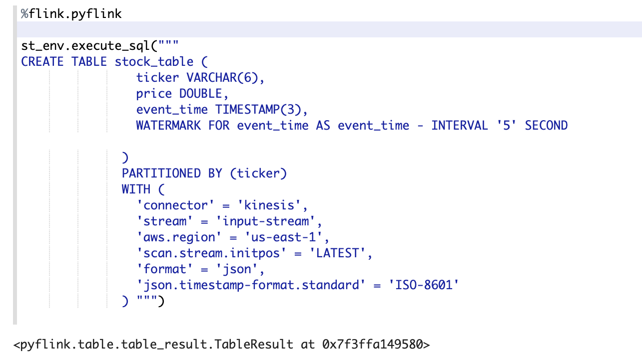
Using the %flink.pyflink header to signify that this code block will be interpreted via the Python Flink interpreter, we’re creating a table called stock_table with a ticker, price, and event_time column that signifies the time at which the price was recorded for the ticker. The WATERMARK clause defines the watermark strategy for generating watermarks according to the event_time (row_time) column. The event_time column must be defined as Timestamp(3) and be a top-level column to be used in conjunction with watermarks. The syntax following the WATERMARK definition—FOR event_time AS event_time - INTERVAL '5' SECOND declares that watermarks will be emitted according to a bounded out of orderness watermark strategy that allows for a five second delay in event_time data.

To learn more about event time and watermarks, read about the techniques implemented by Apache Flink here.

The table defined below uses the Kinesis connector to read from a kinesis data stream called input-stream in the us-east-1 region from the latest stream position.

In this example, we are utilizing the Python interpreter’s built-in streaming table environment variable, st_env, to execute a SQL DDL statement. The streaming table environment provides access to the Table API within pyflink and uses the blink planner to optimize the job graph. This planner translates queries into a DataStream program regardless of whether the input is batch or streaming.

If the table already exists in the AWS Glue Data Catalog, then this statement will issue an error stating that the table already exists.

%flink.pyflink
st_env.execute_sql("""
CREATE TABLE stock_table (
                ticker VARCHAR(6),
                price DOUBLE,
                event_time TIMESTAMP(3),
                WATERMARK FOR event_time AS event_time - INTERVAL '5' SECOND

              )
              PARTITIONED BY (ticker)
              WITH (
                'connector' = 'kinesis',
                'stream' = 'input-stream',
                'aws.region' = 'us-east-1',
                'scan.stream.initpos' = 'LATEST',
                'format' = 'json',
                'json.timestamp-format.standard' = 'ISO-8601'
              ) """)

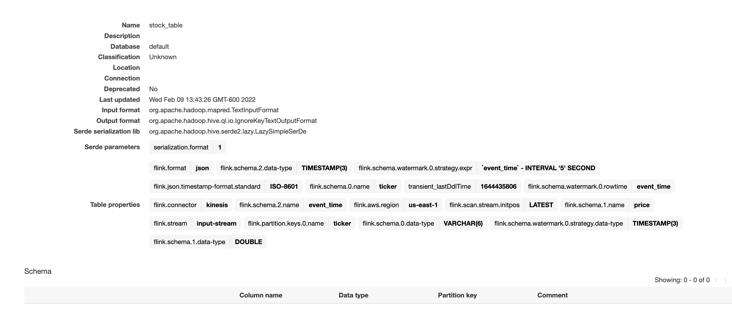
The screenshot above showcases the successful execution of this paragraph. We can verify the results by checking in the AWS Glue Data Catalog for the accompanying table.

To find this, navigate back to the AWS Management Console, and then search for Glue. Once here, locate the Glue database that you chose for our Kinesis Data Analytics application, and select it. You should see a link toward the bottom of the Databases view that lets you view the Tables in your database. Furthermore, you can directly select Tables in the left-hand side. Locate the table that we created in the previous step, called stock_table.

Here we can see that the table was not only created in Kinesis Data Analytics studio, but also durably persisted in a Glue Data Catalog table for reference from other applications or between runs of your application.

Tumbling windows

Performing a tumbling window in the Python Table API first requires the definition of an in-memory reference to the table created in Step 1. We use the st_env variable to define this table using the from_path function and referencing the table name. Once this is created, then we can create a windowed aggregation over one minute of data, according to the event_time column.

Note that you could also perform this transformation entirely in Flink SQL, as described in this blog post. We’re simply showcasing the features of the Pyflink API. The blog post linked above also showcases many different window operators that you might perform, such as sliding windows, group windows, over windows, session windows, etc. The windowing choice is entirely use-case dependent.

%flink.pyflink
from pyflink.table.expressions import col, lit

stock_table = st_env.from_path("stock_table")

 # tumble over 1 minute, then group by that window and sum the number of trades over that time
count_table = stock_table.window(
                     Tumble.over(lit(1).minute).on(stock_table.event_time).alias("one_minute_window")) \
                           .group_by(col("one_minute_window"), col("ticker")) \
                           .select(col("ticker"), col("price").sum.alias("sum_price"), col("one_minute_window").end.alias("minute_window"))

Use the ZeppelinContext to visualize the Python Table aggregation within the notebook.

%flink.pyflink

z.show(count_table, stream_type="update")

This image shows the count_table we defined previously displayed as a pie chart within the Apache Zeppelin notebook.

User-defined functions

To use and reuse common business logic into an operator, it can be useful to reference a User-defined function to transform your Data stream. This can be done either within the Kinesis Data Analytics notebook, or as an externally referenced application jar file. Utilizing User-defined functions can simplify the transformations or data enrichments that you might perform over streaming data.

In our notebook, we will be referencing a simple Java application jar that computes an integer hash of our ticker symbol. You can also write Python or Scala UDFs for use within the notebook. We chose a Java application jar to highlight the functionality of importing an application jar into a Pyflink notebook.

package com.aws.kda.udf;

import org.apache.flink.table.functions.ScalarFunction;

// The Java class must have a public no-argument constructor and can be founded in current Java classloader.
public class HashFunction extends ScalarFunction {
    private int factor = 12;

    public int eval(String s) {
        return s.hashCode() * factor;
    }
    
}

You can find the application jar here.

1. Create and package this jar, or download the link above.
2. Next, upload this application jar to an Amazon S3 bucket to be referenced by our Kinesis Data Analytics Studio notebook.
3. Head back to the Kinesis Data Analytics studio notebook, and under Configuration locate the User-defined functions box. From here, select Add user-defined function, and use the add wizard to locate your uploaded Java jar to reference it.

Once you save changes, the application will take a few minutes to update before you can open it again.

Open the notebook once it has been restarted so that we can reference our UDF.

%flink.pyflink
st_env.create_java_temporary_function("hash", "com.aws.kda.udf.HashFunction")

hash_ticker = stock_table.select("ticker, hash(ticker) as secret_ticker_key, event_time")

Now we can view this newly transformed data from the hash_ticker table context.

%flink.pyflink
st_env.create_java_temporary_function("hash", "com.aws.kda.udf.HashFunction")

hash_ticker = stock_table.select("ticker, hash(ticker) as secret_ticker_key, event_time")

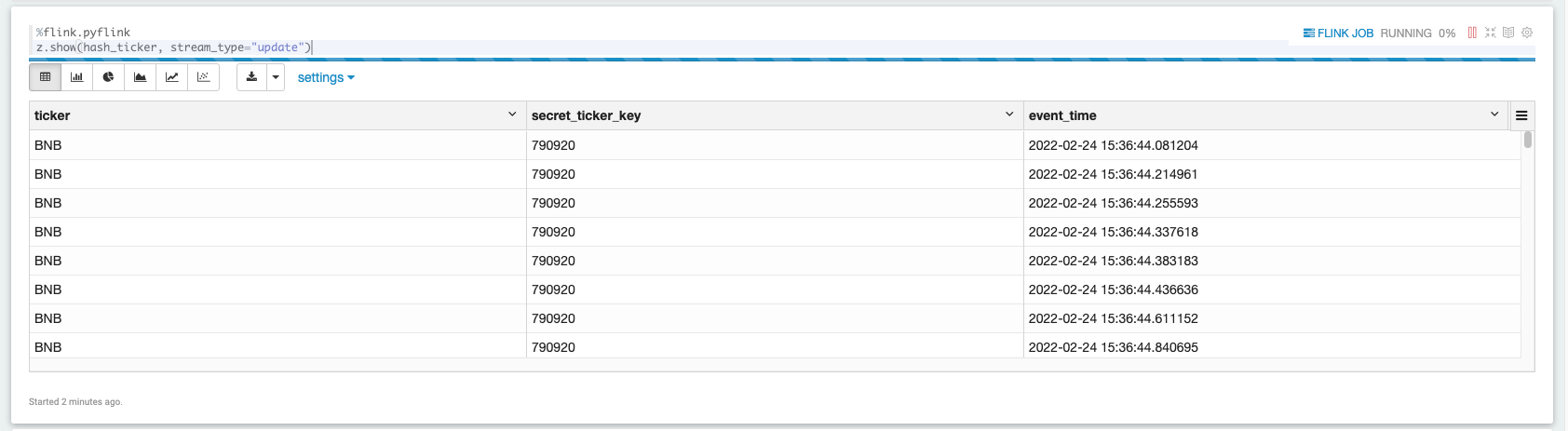
The screenshot above showcases data being displayed in a tabular format from our hashed results set.

Enable checkpointing

To utilize the fault-tolerant features of the Streaming File Sink (writing data to Amazon S3), we must enable checkpointing within our Apache Flink application. This setting isn’t enabled by default on any Kinesis Data Analytics Studio notebook. However, it can be enabled by simply accessing the streaming environment variable’s configuration and setting the proper string accordingly:

%flink.pyflink
z.show(hash_ticker, stream_type="update")

Writing results out to Amazon S3

In the same way that we ingested data into Kinesis Data Analytics Studio, we will create another table, called a sink, that will be responsible for taking data within Kinesis Data Analytics Studio and writing it out to Amazon S3 using the Apache Flink Filesystem connector. This connector does require checkpoints to commit data to a Filesystem, hence the previous step.

First, let’s create the table.

%flink.pyflink

table_name = "output_table"
bucket_name = "kda-python-sink-bucket"

st_env.execute_sql("""CREATE TABLE {0} (
                ticker VARCHAR(6),
                price DOUBLE,
                event_time TIMESTAMP(3)
              )
              PARTITIONED BY (ticker)
              WITH (
                  'connector'='filesystem',
                  'path'='s3a://{1}/',
                  'format'='csv',
                  'sink.partition-commit.policy.kind'='success-file',
                  'sink.partition-commit.delay' = '1 min'
              )""".format(
        table_name, bucket_name))

Next, we can perform the insert by calling the streaming table environment’s execute_sql function.

%flink.pyflink
table_result = st_env.execute_sql("INSERT INTO {0} SELECT * FROM {1}".format("output_table", "hash_ticker"))

The return value table_result is a pyflink table TableResult object. This lets you query and interact with the Flink job that is operating in the background.

Since we’ve set our checkpointing interval to one minute, wait at least one minute with data flowing to see data in your Amazon S3 bucket.

To stop the Amazon S3 sink process, run the following cell:

%flink.pyflink
print(table_result.get_job_client().cancel())

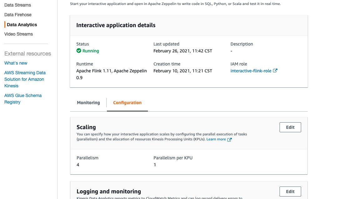
Scaling

A Studio notebook application consists of one or more tasks. You can split an application task into several parallel instances for execution, where each parallel instance processes a subset of the task’s data. The number of parallel instances of a task is called its parallelism, and adjusting that helps execute your tasks more efficiently.

Upon creation, Studio notebooks are given four parallel Kinesis Processing Units (KPU) which make up the application parallelism. To increase that parallelism, navigate to the Kinesis Data Analytics Studio Management Console, select your application name, and select the Configuration tab.

The screenshot above shows the Kinesis Data Analytics Studio console configuration page, where we can note the runtime environment, IAM Role, and modify things like the number of KPU’s the application is allocated.

1. From this page, under the Scaling section, select Edit and modify the Parallelism entry. We don’t recommend increasing the Parallelism Per KPU setting higher than 1 unless your application is I/O bound.
2. Select Save Changes to increase/decrease your application’s parallelism.

Promotion

When you have thoroughly tested and iterated on your application code within a Kinesis Data Analytics Studio notebook, you may choose to promote your notebook to a Kinesis Data Analytics for Apache Flink application with durable state. The benefits of doing this include having full fault tolerance with stateful operations, such as checkpointing, snapshotting, and autoscaling based on CPU usage.

To promote your Kinesis Data Analytics Studio notebook to a Kinesis Data Analytics for Apache Flink application:

1. Navigate to the top-right of your notebook and select Actions for <<notebook name>>.
2. First, select Build <<notebook name>> and export to Amazon S3.
3. Once this process finishes, select Deploy <<notebook name>> as Kinesis Analytics Application. This will open a modal.
4. Then, select Deploy using AWS Console.
5. On the next screen, you can enter the following
   1. An optional description
   2. The same IAM role that you used for your Kinesis Data Analytics Studio notebooks.
6. Then, select Create streaming application. Once the process finishes, you will see a Streaming Application preconfigured with the code supplied by your Kinesis Data Analytics studio notebook.
7. Select Run to start your application.

Make sure that you have stopped all paragraphs in your Kinesis Data Analytics studio notebook so as not to contend for resources with your Kinesis Data Stream.

When the application has started, you should begin to see new data flowing into your Amazon S3 bucket in an entirely fault-tolerant and stateful manner.

Congratulations! You’ve just promoted a Kinesis Data Analytics studio notebook to Kinesis Data Analytics for Apache Flink!

Summary

Kinesis Data Analytics Studio makes developing stream processing applications using Apache Flink much faster. Moreover, all of this is done with rich visualizations, a scalable and user-friendly interface to develop and collaborate on pipelines, and the flexibility of language choice to make any streaming workload performant and powerful. Users can run paragraphs from within the notebook as described in this post, or choose to promote their Studio notebook to a Kinesis Data Analytics for Apache Flink application with durable state.

For more information, please see the following documentation:

• Developer Documentation for Kinesis Data Analytics Studio
• Apache Flink
• Flink Interpreter for Apache Zeppelin

About the Author

Jeremy Ber has been working in the telemetry data space for the past five years as a Software Engineer, Machine Learning Engineer, and most recently a Data Engineer. In the past, Jeremy has supported and built systems that stream in terabytes of data-per-day, and process complex Machine Learning Algorithms in real-time. At AWS, he is a Solutions Architect Streaming Specialist supporting both Managed Streaming for Kafka (Amazon MSK) and Amazon Kinesis services.