Post Syndicated from Crosstalk Solutions original https://www.youtube.com/watch?v=53vN-VmFdi0
Reolink Duo First Look – Dual Lens Camera – Wide viewing angle!
Post Syndicated from digiblurDIY original https://www.youtube.com/watch?v=DUsxNd9Ex6k
Detect Adversary Behavior in Milliseconds with CrowdStrike and Amazon EventBridge
Post Syndicated from Joby Bett original https://aws.amazon.com/blogs/architecture/detect-adversary-behavior-in-seconds-with-crowdstrike-and-amazon-eventbridge/
By integrating Amazon EventBridge with Falcon Horizon, CrowdStrike has developed a real-time, cloud-based solution that allows you to detect threats in less than a second. This solution uses AWS CloudTrail and EventBridge. CloudTrail allows governance, compliance, operational auditing, and risk auditing of your AWS account. EventBridge is a serverless event bus that makes it easier to build event-driven applications at scale.
In this blog post, we’ll cover the challenges presented by using traditional log file-based security monitoring. We will also discuss how CrowdStrike used EventBridge to create an innovative, real-time cloud security solution that enables high-speed, event-driven alerts that detect malicious actors in milliseconds.
Challenges of log file-based security monitoring
Being able to detect malicious actors in your environment is necessary to stay secure in the cloud. With the growing volume, velocity, and variety of cloud logs, log file-based monitoring makes it difficult to reveal adverse behaviors in time to stop breaches.
When an attack is in progress, a security operations center (SOC) analyst has an average of one minute to detect the threat, ten minutes to understand it, and one hour to contain it. If you cannot meet this 1/10/60 minute rule, you may have a costly breach that may move laterally and explode exponentially across the cloud estate.
Let’s look at a real-life scenario. When a malicious actor attempts a ransom attack that targets high-value data in an Amazon Simple Storage Service (Amazon S3) bucket, it can involve activities in various parts of the cloud services in a brief time window.
These example activities can involve:
- AWS Identity and Access Management (IAM): account enumeration, disabling multi-factor authentication (MFA), account hijacking, privilege escalation, etc.
- Amazon Elastic Compute Cloud (Amazon EC2): instance profile privilege escalation, file exchange tool installs, etc.
- Amazon S3: bucket and object enumeration; impair bucket encryption and versioning; bucket policy manipulation; getObject, putObject, and deleteObject APIs, etc.
With siloed log file-based monitoring, detecting, understanding, and containing a ransom attack while still meeting the 1/10/60 rule is difficult. This is because log files are written in batches, and files are typically only created every 5 minutes. Once the log file is written, it still needs to be fetched and processed. This means that you lose the ability to dynamically correlate disparate activities.
To summarize, top-level challenges of log file-based monitoring are:
- Lag time between the breach and the detection
- Inability to correlate disparate activities to reveal sophisticated attack patterns
- Frequent false positive alarms that obscure true positives
- High operational cost of log file synchronizations and reprocessing
- Log analysis tool maintenance for fast growing log volume
Security and compliance is a shared responsibility between AWS and the customer. We protect the infrastructure that runs all of the services offered in the AWS Cloud. For abstracted services, such as Amazon S3, we operate the infrastructure layer, the operating system, and platforms, and customers access the endpoints to store and retrieve data.
You are responsible for managing your data (including encryption options), classifying assets, and using IAM tools to apply the appropriate permissions.
Indicators of attack by CrowdStrike with Amazon EventBridge
In real-world cloud breach scenarios, timeliness of observation, detection, and remediation is critical. CrowdStrike Falcon Horizon IOA is built on an event-driven architecture based on EventBridge and operates at a velocity that can outpace attackers.
CrowdStrike Falcon Horizon IOA performs the following core actions:
- Observe: EventBridge streams CloudTrail log files across accounts to the CrowdStrike platform as activity occurs. Parallelism is enabled via event bus rules, which enables CrowdStrike to avoid the five-minute lag in fetching the log files and dynamically correlate disparate activities. The CrowdStrike platform observes end-to-end activities from AWS services and infrastructure hosted in the accounts protected by CrowdStrike.
- Detect: Falcon Horizon invokes indicators of attack (IOA) detection algorithms that reveal adversarial or anomalous activities from the log file streams. It correlates new and historical events in real time while enriching the events with CrowdStrike threat intelligence data. Each IOA is prioritized with the likelihood of activity being malicious via scoring and mapped to the MITRE ATT&CK framework.
- Remediate: The detected IOA is presented with remediation steps. Depending on the score, applying the remediations quickly can be critical before the attack spreads.
- Prevent: Unremediated insecure configurations are revealed via indicators of misconfiguration (IOM) in Falcon Horizon. Applying the remediation steps from IOM can prevent future breaches.
Key differentiators of IOA from Falcon Horizon are:
- Observability of wider attack surfaces with heterogeneous event sources
- Detection of sophisticated tactics, techniques, and procedures (TTPs) with dynamic event correlation
- Event enrichment with threat intelligence that aids prioritization and reduces alert fatigue
- Low latency between malicious activity occurrence and corresponding detection
- Insight into attacks for each adversarial event from MITRE ATT&CK framework
High-level architecture
Event-driven architectures provide advantages for integrating varied systems over legacy log file-based approaches. For securing cloud attack surfaces against the ever-evolving TTPs, a robust event-driven architecture at scale is a key differentiator.
CrowdStrike maximizes the advantages of event-driven architecture by integrating with EventBridge, as shown in Figure 1. EventBridge allows observing CloudTrail logs in event streams. It also simplifies log centralization from a number of accounts with its direct source-to-target integration across accounts, as follows:
- CrowdStrike hosts an EventBridge with central event buses that consume the stream of CloudTrail log events from a multitude of customer AWS accounts.
- Within customer accounts, EventBridge rules listen to the local CloudTrail and stream each activity as an event to the centralized EventBridge hosted by CrowdStrike.
- CrowdStrike’s event-driven platform detects adversarial behaviors from the event streams in real time. The detection is performed against incoming events in conjunction with historical events. The context that comes from connecting new and historical events minimizes false positives and improves alert efficacy.
- Events are enriched with CrowdStrike threat intelligence data that provides additional insight of the attack to SOC analysts and incident responders.

Figure 1. CrowdStrike Falcon Horizon IOA architecture
As data is received by the centralized EventBridge, CrowdStrike relies on unique customer ID and AWS Region in each event to provide integrity and isolation.
EventBridge allows relatively hassle-free customer onboarding by using cross account rules to transfer customer CloudTrail data into one common event bus that can then be used to filter and selectively forward the data into the Falcon Horizon platform for analysis and mitigation.
Conclusion
As your organization’s cloud footprint grows, visibility into end-to-end activities in a timely manner is critical for maintaining a safe environment for your business to operate. EventBridge allows event-driven monitoring of CloudTrail logs at scale.
CrowdStrike Falcon Horizon IOA, powered by EventBridge, observes end-to-end cloud activities at high speeds at scale. Paired with targeted detection algorithms from in-house threat detection experts and threat intelligence data, Falcon Horizon IOA combats emerging threats against the cloud control plane with its cutting-edge event-driven architecture.
Related information
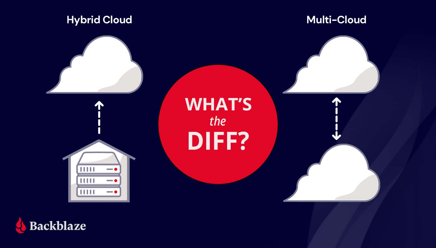
What’s the Diff: Hybrid Cloud vs. Multi-cloud
Post Syndicated from Molly Clancy original https://www.backblaze.com/blog/whats-the-diff-hybrid-cloud-vs-multi-cloud/
For as often as the terms multi-cloud and hybrid cloud get misused, it’s no wonder the concepts put a lot of very smart heads in a spin. The differences between a hybrid cloud and a multi-cloud strategy are simple, but choosing between the two models can have big implications for your business.
In this post, we’ll explain the difference between hybrid cloud and multi-cloud, describe some common use cases, and walk through some ways to get the most out of your cloud deployment.
What’s the Diff: Hybrid Cloud vs. Multi-cloud
Both hybrid cloud and multi-cloud strategies spread data over, you guessed it, multiple clouds. The difference lies in the type of cloud environments—public or private—used to do so. To understand the difference between hybrid cloud and multi-cloud, you first need to understand the differences between the two types of cloud environments.
A public cloud is operated by a third party vendor that sells data center resources to multiple customers over the internet. Much like renting an apartment in a high rise, tenants rent computing space and benefit from not having to worry about upkeep and maintenance of computing infrastructure. In a public cloud, your data may be on the same server as another customer, but it’s virtually separated from other customers’ data by the public cloud’s software layer. Companies like Amazon, Microsoft, Google, and us here at Backblaze are considered public cloud providers.
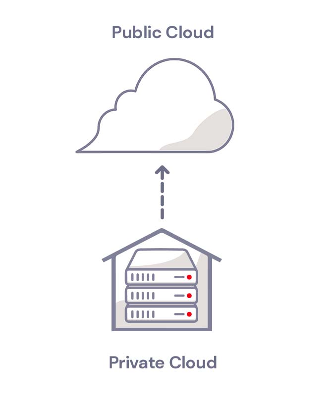
A private cloud, on the other hand, is akin to buying a house. In a private cloud environment, a business or organization typically owns and maintains all the infrastructure, hardware, and software to run a cloud on a private network.
Private clouds are usually built on-premises, but can be maintained off-site at a shared data center. You may be thinking, “Wait a second, that sounds a lot like a public cloud.” You’re not wrong. The key difference is that, even if your private cloud infrastructure is physically located off-site in a data center, the infrastructure is dedicated solely to you and typically protected behind your company’s firewall.
What Is Hybrid Cloud Storage?
A hybrid cloud strategy uses a private cloud and public cloud in combination. Most organizations that want to move to the cloud get started with a hybrid cloud deployment. They can move some data to the cloud without abandoning on-premises infrastructure right away.
A hybrid cloud deployment also works well for companies in industries where data security is governed by industry regulations. For example, the banking and financial industry has specific requirements for network controls, audits, retention, and oversight. A bank may keep sensitive, regulated data on a private cloud and low-risk data on a public cloud environment in a hybrid cloud strategy. Like financial services, health care providers also handle significant amounts of sensitive data and are subject to regulations like the Health Insurance Portability and Accountability Act (HIPAA), which requires various security safeguards where a hybrid cloud is ideal.
A hybrid cloud model also suits companies or departments with data-heavy workloads like media and entertainment. They can take advantage of high-speed, on-premises infrastructure to get fast access to large media files and store data that doesn’t need to be accessed as frequently—archives and backups, for example—with a scalable, low-cost public cloud provider.
Hybrid Cloud
What Is Multi-cloud Storage?
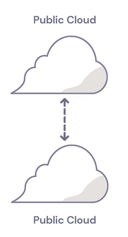
A multi-cloud strategy uses two or more public clouds in combination. A multi-cloud strategy works well for companies that want to avoid vendor lock-in or achieve data redundancy in a failover scenario. If one cloud provider experiences an outage, they can fall back on a second cloud provider.
Companies with operations in countries that have data residency laws also use multi-cloud strategies to meet regulatory requirements. They can run applications and store data in clouds that are located in specific geographic regions.
Multi-cloud
For more information on multi-cloud strategies, check out our Multi-cloud Architecture Guide.
Ways to Make Your Cloud Storage More Efficient
Whether you use hybrid cloud storage or multi-cloud storage, it’s vital to manage your cloud deployment efficiently and manage costs. To get the most out of your cloud strategy, we recommend the following:
- Know your cost drivers. Cost management is one of the biggest challenges to a successful cloud strategy. Start by understanding the critical elements of your cloud bill. Track cloud usage from the beginning to validate costs against cloud invoices. And look for exceptions to historical trends (e.g., identify departments with a sudden spike in cloud storage usage and find out why they are creating and storing more data).
- Identify low-latency requirements. Cloud data storage requires transmitting data between your location and the cloud provider. While cloud storage has come a long way in terms of speed, the physical distance can still lead to latency. The average professional who relies on email, spreadsheets, and presentations may never notice high latency. However, a few groups in your company may require low latency data storage (e.g., HD video editing). For those groups, it may be helpful to use a hybrid cloud approach.
- Optimize your storage. If you use cloud storage for backup and records retention, your data consumption may rise significantly over time. Create a plan to regularly clean your data to make sure data is being correctly deleted when it is no longer needed.
- Prioritize security. Investing up-front time and effort in a cloud security configuration pays off. At a minimum, review cloud provider-specific training resources. In addition, make sure you apply traditional access management principles (e.g., deleting inactive user accounts after a defined period) to manage your risks.
How to Choose a Cloud Strategy
To decide between hybrid cloud storage and multi-cloud storage, consider the following questions:
- Low latency needs. Does your business need low latency capabilities? If so, a hybrid cloud solution may be best.
- Geographical considerations. Does your company have offices in multiple locations and countries with data residency regulations? In that case, a multi-cloud storage strategy with data centers in several countries may be helpful.
- Regulatory concerns. If there are industry-specific requirements for data retention and storage, these requirements may not be fulfilled equally by all cloud providers. Ask the provider how exactly they help you meet these requirements.
- Cost management. Pay close attention to pricing tiers at the outset, and ask the provider what tools, reports, and other resources they provide to keep costs well managed.
Still wondering what type of cloud strategy is right for you? Ask away in the comments.
The post What’s the Diff: Hybrid Cloud vs. Multi-cloud appeared first on Backblaze Blog | Cloud Storage & Cloud Backup.
Security updates for Tuesday
Post Syndicated from original https://lwn.net/Articles/869923/rss
Security updates have been issued by Debian (webkit2gtk, wpewebkit, and xen), Oracle (kernel), Red Hat (curl, go-toolset:rhel8, krb5, mysql:8.0, nodejs:12, and nss and nspr), and Ubuntu (curl and tiff).
Clarity vs Dehaze vs Texture
Post Syndicated from Matt Granger original https://www.youtube.com/watch?v=R6lzorF_b50
Rapid7 Statement on the New Standard Contractual Clauses for International Transfers of Personal Data
Post Syndicated from Chelsea Portney original https://blog.rapid7.com/2021/09/21/rapid7-statement-on-the-new-standard-contractual-clauses-for-international-transfers-of-personal-data/

Context: On June 4, 2021, the European Commission published new standard contractual clauses (“New SCCs”). Under the General Data Protection Regulation (“GDPR”), transfers of personal data to countries outside of the European Economic Area (EEA) must meet certain conditions. The New SCCs are an approved mechanism to enable companies transferring personal data outside of the EEA to meet those conditions, and they replace the previous set of standard contractual clauses (“Old SCCs”), which were deemed inadequate by the Court of Justice of the European Union (“CJEU”). The New SCCs made a number of improvements to the previous version, including but not limited to (i) a modular design which allows parties to choose the module applicable to the personal data being transferred, (ii) use by non-EEA data exporters, and (iii) strengthened data subjects rights and protections.
Rapid7 Action: In light of the European Commission’s adoption of the New SCCs, Rapid7 performed a thorough assessment of its personal data transfers which involved reviewing the technical, contractual, and organizational measures we have in place, evaluating local laws where the personal data will be transferred, and analyzing the necessity for the transfers in accordance with the type and scope of the personal data being transferred. Rapid7 will be updating our Data Processing Addendum on September 27, 2021, to incorporate the New SCCs, where required, for the transfer of personal data outside of the EEA. Rapid7’s adoption of the New SCCs helps ensure we are able to continue to serve all our clients in compliance with GDPR data transfer rules.
Ongoing Commitments: Rapid7 is committed to upholding high standards of privacy and security for our customers, and we are pleased to be able to offer the New SCCs which provide enhanced protections that better take account of the rapidly evolving data environment. We will continue to monitor ongoing changes in order to comply with applicable law and will regularly assess our technical, contractual, and organizational measures in an effort to improve our data protection safeguards. For information on how Rapid7 collects, uses, and discloses personal data, as well as the choices available regarding personal data collected by Rapid7, please see the Rapid7 Privacy Policy. Additionally, Rapid7 remains dedicated to maintaining and enhancing our robust security and privacy program which is outlined in detail on our Trust page.
For more information about our security and privacy program, please email [email protected].
Agentless Oracle database monitoring with ODBC
Post Syndicated from Aigars Kadiķis original https://blog.zabbix.com/agentless-oracle-database-monitoring-with-odbc/15589/
Did you know that Zabbix has an out-of-the-box template for collecting Oracle database metrics? With this template, we can collect data like database, tablespace, ASM, and many other metrics agentlessly, by using ODBC. This blog post will guide you on how to set up ODBC monitoring for Oracle 11.2, 12.1, 18.5, or 19.2 database servers. This post can serve as the perfect set of guidelines for deploying Oracle database monitoring in your environment.
Download Instant client and SQLPlus
The provided commands apply for the following operating systems: CentOS 8, Oracle Linux 8, or Rocky Linux.
First we have to download the following packages:
oracle-instantclient19.12-basic-19.12.0.0.0-1.x86_64.rpm
oracle-instantclient19.12-sqlplus-19.12.0.0.0-1.x86_64.rpm
oracle-instantclient19.12-odbc-19.12.0.0.0-1.x86_64.rpm
Here we are downloading
Oracle instant client – required, to establish connectivity to an Oracle database
SQLPlus – A tool that we can use to test the connectivity to an Oracle database
Oracle ODBC package – contains the required ODBC drivers and configuration scripts to enable ODBC connectivity to an Oracle database
Upload the packages to the Zabbix server (or proxy, if you wish to monitor your Oracle DB on a proxy) and place it in:
/tmp/oracle-instantclient19.12-basic-19.12.0.0.0-1.x86_64.rpm
/tmp/oracle-instantclient19.12-sqlplus-19.12.0.0.0-1.x86_64.rpm
/tmp/oracle-instantclient19.12-odbc-19.12.0.0.0-1.x86_64.rpm
Solve OS dependencies
Install ‘libaio’ and ‘libnsl’ library:
dnf -y install libaio-devel libnsl
Otherwise, we will receive errors:
# rpm -ivh /tmp/oracle-instantclient19.12-basic-19.12.0.0.0-1.x86_64.rpm
error: Failed dependencies:
        libaio is needed by oracle-instantclient19.12-basic-19.12.0.0.0-1.x86_64
        libnsl.so.1()(64bit) is needed by oracle-instantclient19.12-basic-19.12.0.0.0-1.x86_64
# rpm -ivh /tmp/oracle-instantclient19.12-basic-19.12.0.0.0-1.x86_64.rpm
error: Failed dependencies:
        libnsl.so.1()(64bit) is needed by oracle-instantclient19.12-basic-19.12.0.0.0-1.x86_64
Check if Oracle components have been previously deployed on the system. The commands below should provide an empty output:
rpm -qa | grep oracle
ldconfig -p | grep oracle
Install Oracle Instant Client
rpm -ivh /tmp/oracle-instantclient19.12-basic-19.12.0.0.0-1.x86_64.rpm
Make sure that the package ‘oracle-instantclient19.12-basic-19.12.0.0.0-1.x86_64’ is installed:
rpm -qa | grep oracle
LD config
The official Oracle template page at git.zabbix.com talks about the method to configure Oracle ENV Usage for the service. For this version 19.12 of instant client, it is NOT REQUIRED to create a ‘/etc/sysconfig/zabbix-server’ file with content:
export ORACLE_HOME=/usr/lib/oracle/19.12/client64
export PATH=$PATH:$ORACLE_HOME/bin
export LD_LIBRARY_PATH=$ORACLE_HOME/lib:/usr/lib64:/usr/lib:$ORACLE_HOME/bin
export TNS_ADMIN=$ORACLE_HOME/network/admin
While we did install the rpm package, the Oracle 19.12 client package did auto-configure LD path at the global level – it means every user on the system can use the Oracle instant client. We can see the LD path have been configured under:
cat /etc/ld.so.conf.d/oracle-instantclient.conf
This will print:
/usr/lib/oracle/19.12/client64/lib
To ensure that the required Oracle libraries are recognized by the OS, we can run:
ldconfig -p | grep oracle
It should print:
liboramysql19.so (libc6,x86-64) => /usr/lib/oracle/19.12/client64/lib/liboramysql19.so
libocijdbc19.so (libc6,x86-64) => /usr/lib/oracle/19.12/client64/lib/libocijdbc19.so
libociei.so (libc6,x86-64) => /usr/lib/oracle/19.12/client64/lib/libociei.so
libocci.so.19.1 (libc6,x86-64) => /usr/lib/oracle/19.12/client64/lib/libocci.so.19.1
libnnz19.so (libc6,x86-64) => /usr/lib/oracle/19.12/client64/lib/libnnz19.so
libmql1.so (libc6,x86-64) => /usr/lib/oracle/19.12/client64/lib/libmql1.so
libipc1.so (libc6,x86-64) => /usr/lib/oracle/19.12/client64/lib/libipc1.so
libclntshcore.so.19.1 (libc6,x86-64) => /usr/lib/oracle/19.12/client64/lib/libclntshcore.so.19.1
libclntshcore.so (libc6,x86-64) => /usr/lib/oracle/19.12/client64/lib/libclntshcore.so
libclntsh.so.19.1 (libc6,x86-64) => /usr/lib/oracle/19.12/client64/lib/libclntsh.so.19.1
libclntsh.so (libc6,x86-64) => /usr/lib/oracle/19.12/client64/lib/libclntsh.so
Note: If for some reason the ldconfig command shows links to other dynamic libraries – that’s when we might have to create a separate ENV file for Zabbix server/Proxy, which would link the Zabbix application to the correct dynamic libraries, as per the example at the start of this section.
Check if the Oracle service port is reachable
To save us some headache down the line, let’s first check the network connectivity to our Oracle database host. Let’s check if we can reach the default Oracle port at the network level. In this example, we will try to connect to the default Oracle database port, 1521. Depending on which port your Oracle database is listening for connections, adjust accordingly,. Make sure the output says ‘Connected to 10.1.10.15:1521’:
nc -zv 10.1.10.15 1521
Test connection with SQLPlus
We can simulate the connection to the Oracle database before moving on with the ODBC configuration. Make sure that the Oracle username and password used in the command are correct. For this task, we will first need to install the SQLPlus package.:
rpm -ivh /tmp/oracle-instantclient19.12-sqlplus-19.12.0.0.0-1.x86_64.rpm
To simulate the connection, we can use a one-liner command. In the example command I’m using the username ‘system’ together with the password ‘oracle’ to reach out to the Oracle database server ‘10.1.10.15’ via port ‘1521’ and connect to the service name ‘xe’:
sqlplus64 'system/oracle@(DESCRIPTION=(ADDRESS_LIST=(ADDRESS=(PROTOCOL=TCP)(HOST=10.1.10.15)(PORT=1521)))(CONNECT_DATA=(SERVER=DEDICATED)(SERVICE_NAME=xe)))'
In the output we can see: we are using the 19.12 client to connect to 11.2 server:
SQL*Plus: Release 19.0.0.0.0 - Production on Mon Sep 6 13:47:36 2021
Version 19.12.0.0.0
Copyright (c) 1982, 2021, Oracle.  All rights reserved.
Connected to:
Oracle Database 11g Express Edition Release 11.2.0.2.0 - 64bit Production
Note: This gives us an extra hint regarding the Oracle instant client – newer versions of the client are backwards compatible with the older versions of the Oracle database server. Though this doesn’t apply to every version of Oracle client/server, please check the Oracle instant client documentation first.
ODBC connector
When it comes to configuring ODBC, let’s first install the ODBC driver manager
dnf -y install unixODBC
Now we can see that we have two new files – ‘/etc/odbc.ini’ (possibly empty) and ‘/etc/odbcinst.ini’.
The file ‘/etc/odbcinst.ini’ describes driver relation. Currently, when we ‘grep’ the keyword ‘oracle’ there is no oracle relation installed, the output is empty when we run:
grep -i oracle /etc/odbcinst.ini
Our next step is to Install Oracle ODBC driver package:
rpm -ivh /tmp/oracle-instantclient19.12-odbc-19.12.0.0.0-1.x86_64.rpm
The ‘oracle-instantclient*-odbc’ package contains a script that will update the ‘/etc/odbcinst.ini’ configuration automatically:
cd /usr/lib/oracle/19.12/client64/bin
./odbc_update_ini.sh / /usr/lib/oracle/19.12/client64/lib
It will print:
*** ODBCINI environment variable not set,defaulting it to HOME directory!
Now when we print the file on the screen:
cat /etc/odbcinst.ini
We will see that there is the Oracle 19 ODBC driver section added at the end of the file::
[Oracle 19 ODBC driver]
Description     = Oracle ODBC driver for Oracle 19
Driver          = /usr/lib/oracle/19.12/client64/lib/libsqora.so.19.1
Setup           =
FileUsage       =
CPTimeout       =
CPReuse         =
It’s important to check if there are no errors produced in the output when executing the ‘ldd’ command. This ensures that the dependencies are satisfied and accessible and there are no conflicts with the library versioning:
ldd /usr/lib/oracle/19.12/client64/lib/libsqora.so.19.1
It will print something similar like:
linux-vdso.so.1 (0x00007fff121b5000)
libdl.so.2 => /lib64/libdl.so.2 (0x00007fb18601c000)
libm.so.6 => /lib64/libm.so.6 (0x00007fb185c9a000)
libpthread.so.0 => /lib64/libpthread.so.0 (0x00007fb185a7a000)
libnsl.so.1 => /lib64/libnsl.so.1 (0x00007fb185861000)
librt.so.1 => /lib64/librt.so.1 (0x00007fb185659000)
libaio.so.1 => /lib64/libaio.so.1 (0x00007fb185456000)
libresolv.so.2 => /lib64/libresolv.so.2 (0x00007fb18523f000)
libclntsh.so.19.1 => /usr/lib/oracle/19.12/client64/lib/libclntsh.so.19.1 (0x00007fb1810e6000)
libclntshcore.so.19.1 => /usr/lib/oracle/19.12/client64/lib/libclntshcore.so.19.1 (0x00007fb180b42000)
libodbcinst.so.2 => /lib64/libodbcinst.so.2 (0x00007fb18092c000)
libc.so.6 => /lib64/libc.so.6 (0x00007fb180567000)
/lib64/ld-linux-x86-64.so.2 (0x00007fb1864da000)
libnnz19.so => /usr/lib/oracle/19.12/client64/lib/libnnz19.so (0x00007fb17fdba000)
libltdl.so.7 => /lib64/libltdl.so.7 (0x00007fb17fbb0000)
When we executed the ‘odbc_update_ini.sh’ script, a new DSN (data source name) file was made in ‘/root/.odbc.ini’. This is a sample configuration ODBC configuration file which describes what settings this version of ODBC driver supports.
Let’s move this configuration file from the user directories to a location accessible system-wide:
cat /root/.odbc.ini | sudo tee -a /etc/odbc.ini
And remove the file from the user directory completely:
rm /root/.odbc.ini
This way, every user in the system will use only this one ODBC configuration file.
We can now alter the existing configuration – /etc/odbc.ini. I’m highlighting things that have been changed from the defaults:
[Oracle11g]
AggregateSQLType = FLOAT
Application Attributes = T
Attributes = W
BatchAutocommitMode = IfAllSuccessful
BindAsFLOAT = F
CacheBufferSize = 20
CloseCursor = F
DisableDPM = F
DisableMTS = T
DisableRULEHint = T
Driver = Oracle 19 ODBC driver
DSN = Oracle11g
EXECSchemaOpt =
EXECSyntax = T
Failover = T
FailoverDelay = 10
FailoverRetryCount = 10
FetchBufferSize = 64000
ForceWCHAR = F
LobPrefetchSize = 8192
Lobs = T
Longs = T
MaxLargeData = 0
MaxTokenSize = 8192
MetadataIdDefault = F
QueryTimeout = T
ResultSets = T
ServerName = //10.1.10.15:1521/xe
SQLGetData extensions = F
SQLTranslateErrors = F
StatementCache = F
Translation DLL =
Translation Option = 0
UseOCIDescribeAny = F
UserID = system
Password = oracle
DNS – Data source name. Should match the section name in brackets, e.g.:[Oracle11g]
ServerName – Oracle server address
UserID – Oracle user name
Password – Oracle user password
To test the connection from the command line, let’s use the isql command-line tool which should simulate the ODBC connection akin to what the Zabbix is doing when gathering metrics:
isql -v Oracle11g
The isql command in this example picks up the ODBC settings (Username, Password, Server address) from the odbc.ini file. All we have to do is reference the particular DSN – Oracle11g
On the other hand, if we do not prefer to keep the password on the filesystem (/etc/odbc.ini), we can erase the lines ‘UserID’ and ‘Password’. Then we can test the ODBC connection with:
isql -v Oracle11g 'system' 'oracle'
In case of a successful connection it should print:
+---------------------------------------+
| Connected!                            |
|                                       |
| sql-statement                         |
| help [tablename]                      |
| quit                                  |
|                                       |
+---------------------------------------+
SQL>
And that’s it for the ODBC configuration! Now we should be able to apply the Oracle by ODBC template in Zabbix

Don’t forget that we also need to provide the necessary Oracle credentials to start collecting Oracle database metrics:

The lessons learned in this blog post can be easily applied to ODBC monitoring and troubleshooting in general, not just Oracle. If you’re having any issues or wish to share your experience with ODBC or Oracle database monitoring – feel free to leave us a comment!
Alaska’s Department of Health and Social Services Hack
Post Syndicated from Bruce Schneier original https://www.schneier.com/blog/archives/2021/09/alaskas-department-of-health-and-social-services-hack.html
Apparently, a nation-state hacked Alaska’s Department of Health and Social Services.
Not sure why Alaska’s Department of Health and Social Services is of any interest to a nation-state, but that’s probably just my failure of imagination.
Automatically tune your guitar with Raspberry Pi Pico
Post Syndicated from Ashley Whittaker original https://www.raspberrypi.org/blog/automatically-tune-your-guitar-with-raspberry-pi-pico/
You sit down with your six-string, ready to bash out that new song you recently mastered, but find you’re out of tune. Redditor u/thataintthis (Guyrandy Jean-Gilles) has taken the pain out of tuning your guitar, so those of us lacking this necessary skill can skip the boring bit and get back to playing.
Before you dismiss this project as just a Raspberry Pi Pico-powered guitar tuning box, read on, because when the maker said this is a fully automatic tuner, they meant it.
How does it work?
Guyrandy’s device listens to the sound of a string being plucked and decides which note it needs to be tuned to. Then it automatically turns the tuning keys on the guitar’s headstock just the right amount until it achieves the correct note.
Genius.
If this were a regular tuning box, it would be up to the musician to fiddle with the tuning keys while twanging the string until they hit a note that matches the one being made by the tuning box.
It’s currently hardcoded to do standard tuning, but it could be tweaked to do things like Drop D tuning.

Upgrade suggestions
Commenters were quick to share great ideas to make this build even better. Issues of harmonics were raised, and possible new algorithms to get around it were shared. Another commenter noticed the maker wrote their own code in C and suggested making use of the existing ulab FFT in MicroPython. And a final great idea was training the Raspberry Pi Pico to accept the guitar’s audio output as input and analyse the note that way, rather than using a microphone, which has a less clear sound quality.
These upgrades seemed to pique the maker’s interest. So maybe watch this space for a v2.0 of this project…
(Watch out for some spicy language in the comments section of the original reddit post. People got pretty lively when articulating their love for this build.)
Inspiration
This project was inspired by the Roadie automatic tuning device. Roadie is sleek but it costs big cash money. And it strips you of the hours of tinkering fun you get from making your own version.
All the code for the project can be found here.
The post Automatically tune your guitar with Raspberry Pi Pico appeared first on Raspberry Pi.
Comic for 2021.09.21
Post Syndicated from Explosm.net original http://explosm.net/comics/5982/
New Cyanide and Happiness Comic
Live Stream with Tediore™ – Wyze LED Strip with ESP32 / MJ Fan Controller
Post Syndicated from digiblurDIY original https://www.youtube.com/watch?v=CDwpxecW700
Live Fan Controller ESP8266 & Water Valve ESP32-C3 Transplants
Post Syndicated from digiblurDIY original https://www.youtube.com/watch?v=ie6SBHvBR0g
Hoyt: Structural pattern matching in Python 3.10
Post Syndicated from original https://lwn.net/Articles/869883/rss
Ben Hoyt has published a critical
overview of the Python 3.10 pattern-matching feature.
As shown above, there are cases where match really
shines. But they are few and far between, mostly when handling
syntax trees and writing parsers. A lot of code does have
if ... elif chains, but these are often either
plain switch-on-value, where elif works almost as well, or
the conditions they’re testing are a more complex combination of
tests that don’t fit into case patterns (unless you use awkward
case _ if cond clauses, but that’s strictly worse than
elif).
(Pattern matching has been covered here as
well).
Accelerate your data warehouse migration to Amazon Redshift – Part 4
Post Syndicated from Michael Soo original https://aws.amazon.com/blogs/big-data/part-4-accelerate-your-data-warehouse-migration-to-amazon-redshift/
This is the fourth in a series of posts. We’re excited to share dozens of new features to automate your schema conversion; preserve your investment in existing scripts, reports, and applications; accelerate query performance; and potentially reduce your overall cost to migrate to Amazon Redshift.
Check out the previous posts in the series:
|
Amazon Redshift is the leading cloud data warehouse. No other data warehouse makes it as easy to gain new insights from your data. With Amazon Redshift, you can query exabytes of data across your data warehouse, operational data stores, and data lake using standard SQL. You can also integrate other AWS services like Amazon EMR, Amazon Athena, Amazon SageMaker, AWS Glue, AWS Lake Formation, and Amazon Kinesis to use all the analytic capabilities in the AWS Cloud.
Many customers have asked for help migrating from self-managed data warehouse engines, like Teradata, to Amazon Redshift. In these cases, you typically have terabytes or petabytes of data, a heavy reliance on proprietary features, and thousands of extract, transform, and load (ETL) processes and reports built over a few years (or decades) of use.
Until now, migrating a data warehouse to AWS was complex and involved a significant amount of manual effort. You needed to manually remediate syntax differences, inject code to replace proprietary features, and manually tune the performance of queries and reports on the new platform.
For example, you may have a significant investment in BTEQ (Basic Teradata Query) scripting for database automation, ETL, or other tasks. Previously, you needed to manually recode these scripts as part of the conversion process to Amazon Redshift. Together with supporting infrastructure (job scheduling, job logging, error handling), this was a significant impediment to migration.
Today, we’re happy to share with you a new, purpose-built command line tool called Amazon Redshift RSQL. Some of the key features added in Amazon Redshift RSQL are enhanced flow control syntax and single sign-on support. You can also describe properties or attributes of external tables in an AWS Glue catalog or Apache Hive Metastore, external databases in Amazon RDS for PostgreSQL or Amazon Aurora PostgreSQL-Compatible Edition, and tables shared using Amazon Redshift data sharing.
We have also enhanced the AWS Schema Conversion Tool (AWS SCT) to automatically convert BTEQ scripts to Amazon Redshift RSQL scripts. The converted scripts run on Amazon Redshift with little to no changes.
In this post, we describe some of the features of Amazon Redshift RSQL, show example scripts, and demonstrate how to convert BTEQ scripts into Amazon Redshift RSQL scripts.
Amazon Redshift RSQL features
If you currently use Amazon Redshift, you may already be running scripts on Amazon Redshift using the PSQL command line client. These scripts operate on Amazon Redshift RSQL with no modification. You can think of Amazon Redshift RSQL as an Amazon Redshift-native version of PSQL.
In addition, we have designed Amazon Redshift RSQL to make it easy to transition BTEQ scripts to the tool. The following are some examples of Amazon Redshift RSQL commands that make this possible. (For full details, see Amazon Redshift RSQL.)
- \EXIT – This command is an extension of the PSQL \quit command. Like \quit, \EXIT terminates the execution of Amazon Redshift RSQL. In addition, you can specify an optional exit code with \EXIT.
- \LOGON – This command creates a new connection to a database. \LOGON is an alias for the PSQL \connect command. You can specify connection parameters using positional syntax or as a connection string.
- \REMARK – This command prints the specified string to the output. \REMARK extends the PSQL \echo command by adding the ability to break the output over multiple lines, using // as a line break.
- \RUN – This command runs the Amazon Redshift RSQL script contained in the specified file. \RUN extends the PSQL \i command by adding an option to skip any number of lines in the specified file.
- \OS – This is an alias for the PSQL \! command. \OS runs the operating system command that is passed as a parameter. Control returns to Amazon Redshift RSQL after running the OS command.
- \LABEL – This is a new command for Amazon Redshift RSQL. \LABEL establishes an entry point for execution, as the target for a \GOTO command.
- \GOTO – This command is a new command for Amazon Redshift RSQL. It’s used in conjunction with the \LABEL command. \GOTO skips all intervening commands and resumes processing at the specified \LABEL. The \LABEL must be a forward reference. You can’t jump to a \LABEL that lexically precedes the \GOTO.
- \IF (\ELSEIF, \ELSE, \ENDIF) – This command is an extension of the PSQL \if (\elif, \else, \endif) command. \IF and \ELSEIF support arbitrary Boolean expressions including AND, OR, and NOT conditions. You can use the \GOTO command within a \IF block to control conditional execution.
- \EXPORT – This command specifies the name of an export file that Amazon Redshift RSQL uses to store database information returned by a subsequent SQL SELECT statement.
We’ve also added some variables to Amazon Redshift RSQL to support converting your BTEQ scripts.
- :ACTIVITYCOUNT – This variable returns the number of rows affected by the last submitted request. For a data-returning request, this is the number of rows returned to Amazon Redshift RSQL from the database. ACTIVITYCOUNT is similar to the PSQL variable ROW_COUNT, however, ROW_COUNT does not report affected-row count for SELECT, COPY or UNLOAD.
- :ERRORCODE – This variable contains the return code for the last submitted request to the database. A zero signifies the request completed without error. The ERRORCODE variable is an alias for the variable SQLSTATE.
- :ERRORLEVEL – This variable assigns severity levels to errors. Use the severity levels to determine a course of action based on the severity of the errors that Amazon Redshift RSQL encounters.
- :MAXERROR – This variable designates a maximum error severity level beyond which Amazon Redshift RSQL terminates job processing.
An example Amazon Redshift RSQL script
Let’s look at an example. First, we log in to an Amazon Redshift database using Amazon Redshift RSQL. You specify the connection information on the command line as shown in the following code. The port and database are optional and default to 5439 and dev respectively if not provided.
If you choose to change the connection from within the client, you can use the \LOGON command:
Now, let’s run a simple script that runs a SELECT statement, checks for output, then branches depending on whether data was returned or not.
First, we inspect the script by using the \OS command to print the file to the screen:
The script prints one of two messages depending on whether data is returned by the SELECT statement or not.
Now, let’s run the script using the \RUN command. The SELECT statement returns 11 rows of data. The script prints a “data found” message, and jumps to the LETSDOSOMETHING label.
That’s Amazon Redshift RSQL in a nutshell. If you’re developing new scripts for Amazon Redshift, we encourage you to use Amazon Redshift RSQL and take advantage of its additional capabilities. If you have existing PSQL scripts, you can run those scripts using Amazon Redshift RSQL with no changes.
Use AWS SCT to automate your BTEQ conversions
If you’re a Teradata developer or DBA, you’ve probably built a library of BTEQ scripts that you use to perform administrative work, load or transform data, or to generate datasets and reports. If you’re contemplating a migration to Amazon Redshift, you’ll want to preserve the investment you made in creating those scripts.
AWS SCT has long had the ability to convert BTEQ to AWS Glue. Now, you can also use AWS SCT to automatically convert BTEQ scripts to Amazon Redshift RSQL. AWS SCT supports all the new Amazon Redshift RSQL features like conditional execution, escape to the shell, and branching.
Let’s see how it works. We create two Teradata tables, product_stg and product. Then we create a simple ETL script that uses a MERGE statement to update the product table using data from the product_stg table:
We embed the MERGE statement inside a BTEQ script. The script tests error conditions and branches accordingly:
Now, let’s use AWS SCT to convert the script to Amazon Redshift RSQL. AWS SCT converts the BTEQ commands to their Amazon Redshift RSQL and Amazon Redshift equivalents. The converted script is as follows:
The following are the main points of interest in the conversion:
- The BTEQ .SET WIDTH command is converted to the Amazon Redshift RSQL \RSET WIDTH command.
- The BTEQ ACTIVITYCOUNT variable is converted to the Amazon Redshift RSQL ACTIVITYCOUNT variable.
- The BTEQ MERGE statement is converted into an UPDATE followed by an INSERT statement. Currently, Amazon Redshift doesn’t support a native MERGE statement.
- The BTEQ .LABEL and .GOTO statements are translated to their Amazon Redshift RSQL equivalents \LABEL and \GOTO.
Let’s look at the actual process of using AWS SCT to convert a BTEQ script.
After starting AWS SCT, you create a Teradata migration project and navigate to the BTEQ scripts node in the source tree window pane. Right-click and choose Load scripts.
Then select the folder that contains your BTEQ scripts. The folder appears in the source tree. Open it and navigate to the script you want to convert. In our case, the script is contained in the file merge.sql. Right-click on the file, choose Convert script, then choose Convert to RSQL. You can inspect the converted script in the bottom middle pane. When you’re ready to save the script to a file, do that from the target tree on the right side.
If you have many BTEQ scripts, you can convert an entire folder at once by selecting the folder instead of an individual file.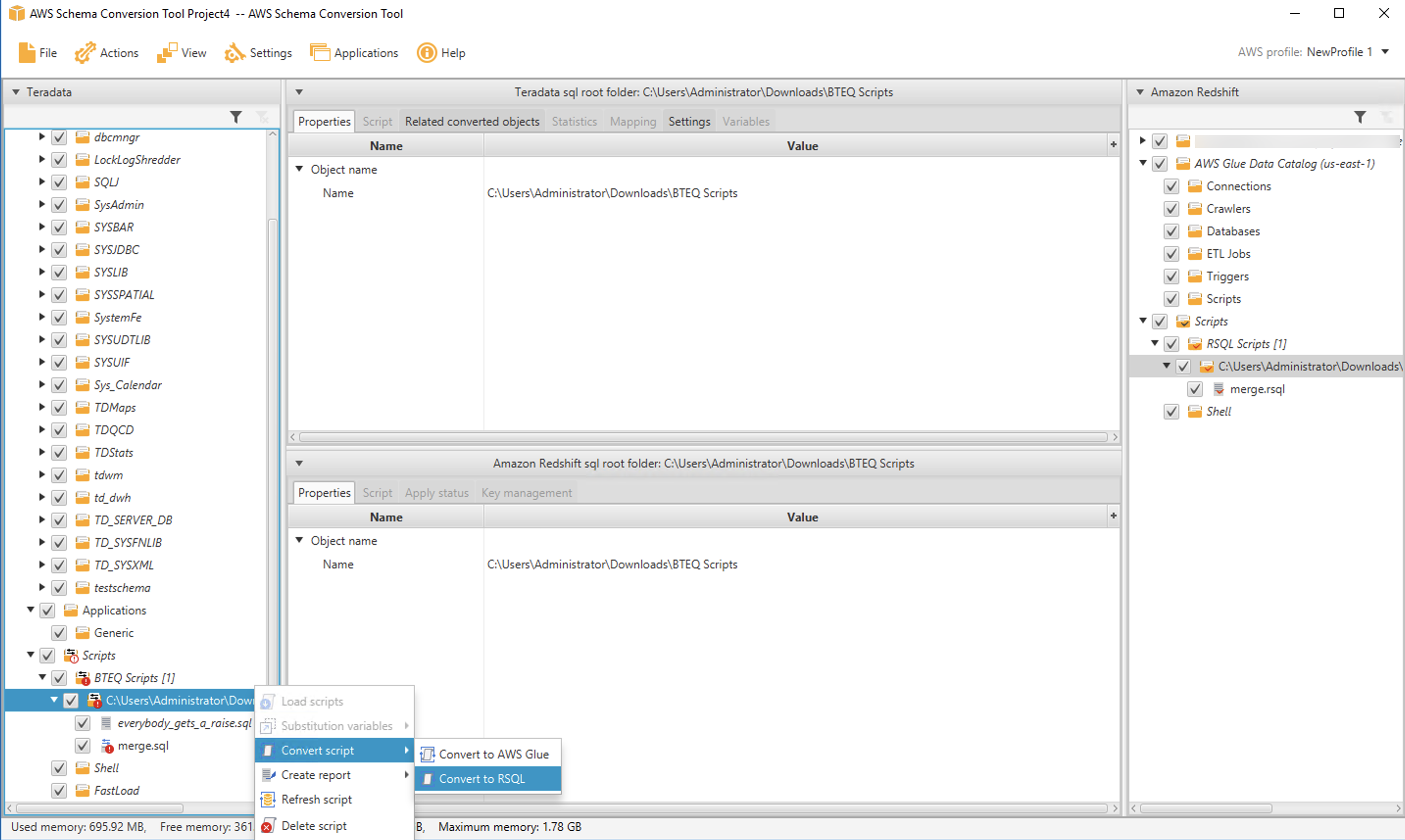
Convert shell scripts
Many applications run BTEQ commands from within shell scripts. For example, you may have a shell script that redirects log output and controls login credentials, as in the following:
If you use shell scripts to run BTEQ, we’re happy to share that AWS SCT can help you convert those scripts. AWS SCT supports bash scripts now, and we’ll add additional shell dialects in the future.
The process to convert shell scripts is very similar to BTEQ conversion. You select a folder that contains your scripts by navigating to the Shell node in the source tree and then choosing Load scripts.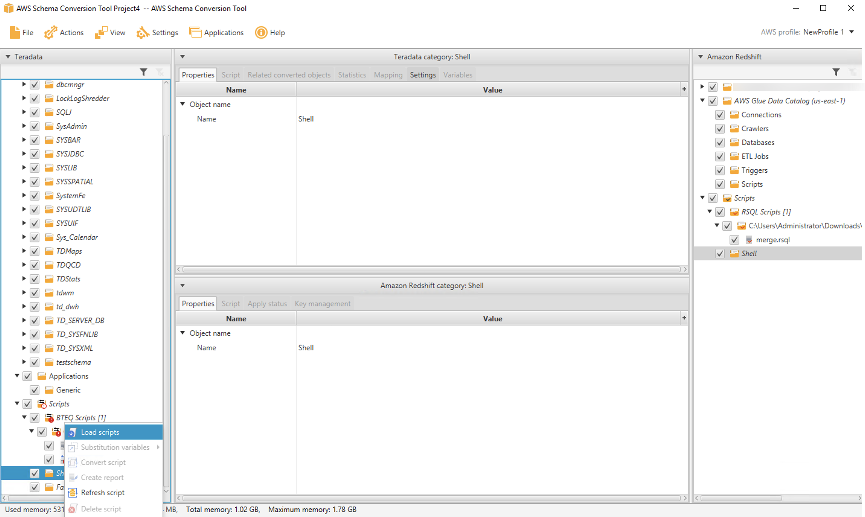
After the folder is loaded, you can convert one (or more) scripts by selecting them and choosing Convert script.
As before, the converted script appears in the UI, and you can save it from the target tree on the right side of the page.
Conclusion
We’re happy to share Amazon Redshift RSQL and expect it to be a big hit with customers. If you’re contemplating a migration from Teradata to Amazon Redshift, Amazon Redshift RSQL and AWS SCT can simplify the conversion of your existing Teradata scripts and help preserve your investment in existing reports, applications, and ETL.
All of the features described in this post are available for you to use today. You can download Amazon Redshift RSQL and AWS SCT and give it a try.
We’ll be back soon with the next installment in this series. Check back for more information on automating your migrations from Teradata to Amazon Redshift. In the meantime, you can learn more about Amazon Redshift, Amazon Redshift RSQL, and AWS SCT. Happy migrating!
About the Authors
 Michael Soo is a Senior Database Engineer with the AWS Database Migration Service team. He builds products and services that help customers migrate their database workloads to the AWS cloud.
 Po Hong, PhD, is a Principal Data Architect of Lake House Global Specialty Practice,
AWS Professional Services. He is passionate about supporting customers to adopt innovative solutions to reduce time to insight. Po is specialized in migrating large scale MPP on-premises data warehouses to the AWS Lake House architecture.
 Entong Shen is a Software Development Manager of Amazon Redshift. He has been working on MPP databases for over 9 years and has focused on query optimization, statistics and migration related SQL language features such as stored procedures and data types.
 Adekunle Adedotun is a Sr. Database Engineer with Amazon Redshift service. He has been working on MPP databases for 6 years with a focus on performance tuning. He also provides guidance to the development team for new and existing service features.
 Asia Khytun is a Software Development Manager for the AWS Schema Conversion Tool. She has 10+ years of software development experience in C, C++, and Java.
 Illia Kratsov is a Database Developer with the AWS Project Delta Migration team. He has 10+ years experience in data warehouse development with Teradata and other MPP databases.
Accelerate your data warehouse migration to Amazon Redshift – Part 3
Post Syndicated from Michael Soo original https://aws.amazon.com/blogs/big-data/part-3-accelerate-your-data-warehouse-migration-to-amazon-redshift/
This is the third post in a multi-part series. We’re excited to share dozens of new features to automate your schema conversion; preserve your investment in existing scripts, reports, and applications; accelerate query performance; and reduce your overall cost to migrate to Amazon Redshift.
Check out the previous posts in the series:
|
Amazon Redshift is the leading cloud data warehouse. No other data warehouse makes it as easy to gain new insights from your data. With Amazon Redshift, you can query exabytes of data across your data warehouse, operational data stores, and data lake using standard SQL. You can also integrate other services such as Amazon EMR, Amazon Athena, and Amazon SageMaker to use all the analytic capabilities in the AWS Cloud.
Many customers have asked for help migrating from self-managed data warehouse engines, like Teradata, to Amazon Redshift. In these cases, you may have terabytes (or petabytes) of historical data, a heavy reliance on proprietary features, and thousands of extract, transform, and load (ETL) processes and reports built over years (or decades) of use.
Until now, migrating a Teradata data warehouse to AWS was complex and involved a significant amount of manual effort.
Today, we’re happy to share recent enhancements to Amazon Redshift and the AWS Schema Conversion Tool (AWS SCT) that make it easier to automate your Teradata to Amazon Redshift migrations.
In this post, we introduce new automation for merge statements, a native function to support ASCII character conversion, enhanced error checking for string to date conversion, enhanced support for Teradata cursors and identity columns, automation for ANY and SOME predicates, automation for RESET WHEN clauses, automation for two proprietary Teradata functions (TD_NORMALIZE_OVERLAP and TD_UNPIVOT), and automation to support analytic functions (QUANTILE and QUALIFY).
Merge statement
Like its name implies, the merge statement takes an input set and merges it into a target table. If an input row already exists in the target table (a row in the target table has the same primary key value), then the target row is updated. If there is no matching target row, the input row is inserted into the table.
Until now, if you used merge statements in your workload, you were forced to manually rewrite the merge statement to run on Amazon Redshift. Now, we’re happy to share that AWS SCT automates this conversion for you. AWS SCT decomposes a merge statement into an update on existing records followed by an insert for new records.
Let’s look at an example. We create two tables in Teradata: a target table, employee, and a delta table, employee_delta, where we stage the input rows:
Now we create a Teradata merge statement that updates a row if it exists in the target, otherwise it inserts the new row. We embed this merge statement into a macro so we can show you the conversion process later.
Now we use AWS SCT to convert the macro. (See Accelerate your data warehouse migration to Amazon Redshift – Part 1 for details on macro conversion.) AWS SCT creates a stored procedure that contains an update (to implement the WHEN MATCHED condition) and an insert (to implement the WHEN NOT MATCHED condition).
This example showed how to use merge automation for macros, but you can convert merge statements in any application context: stored procedures, BTEQ scripts, Java code, and more. Download the latest version of AWS SCT and try it out.
ASCII() function
The ASCII function takes as input a string and returns the ASCII code, or more precisely, the UNICODE code point, of the first character in the string. Previously, Amazon Redshift supported ASCII as a leader-node only function, which prevented its use with user-defined tables.
We’re happy to share that the ASCII function is now available on Amazon Redshift compute nodes and can be used with user-defined tables. In the following code, we create a table with some string data:
Now you can use the ASCII function on the string columns:
Lastly, if your application code uses the ASCII function, AWS SCT automatically converts any such function calls to Amazon Redshift.
The ASCII feature is available now—try it out in your own cluster.
TO_DATE() function
The TO_DATE function converts a character string into a DATE value. A quirk of this function is that it can accept a string value that isn’t a valid date and translate it into a valid date.
For example, consider the string 2021-06-31. This isn’t a valid date because the month of June has only 30 days. However, the TO_DATE function accepts this string and returns the “31st” day of June (July 1):
Customers have asked for strict input checking for TO_DATE, and we’re happy to share this new capability. Now, you can include a Boolean value in the function call that turns on strict checking:
You can turn off strict checking explicitly as well:
Also, the Boolean value is optional. If you don’t include it, strict checking is turned off, and you see the same behavior as before the feature was launched.
You can learn more about the TO_DATE function and try out strict date checking in Amazon Redshift now.
CURSOR result sets
A cursor is a programming language construct that applications use to manipulate a result set one row at a time. Cursors are more relevant for OLTP applications, but some legacy applications built on data warehouses also use them.
Teradata provides a diverse set of cursor configurations. Amazon Redshift supports a more streamlined set of cursor features.
Based on customer feedback, we’ve added automation to support Teradata WITH RETURN cursors. These types of cursors are opened within stored procedures and returned to the caller for processing of the result set. AWS SCT will convert a WITH RETURN cursor to an Amazon Redshift REFCURSOR.
For example, consider the following procedure, which contains a WITH RETURN cursor. The procedure opens the cursor and returns the result to the caller as a DYNAMIC RESULT SET:
AWS SCT converts the procedure as follows. An additional parameter is added to the procedure signature to pass the REFCURSOR:
IDENTITY columns
Teradata supports several non-ANSI compliant features for IDENTITY columns. We have enhanced AWS SCT to automatically convert these features to Amazon Redshift, whenever possible.
Specifically, AWS SCT now converts the Teradata START WITH and INCREMENT BY clauses to the Amazon Redshift SEED and STEP clauses, respectively. For example, consider the following Teradata table:
The GENERATED ALWAYS clause indicates that the column is always populated automatically—a value can’t be explicitly inserted or updated into the column. The START WITH clause defines the first value to be inserted into the column, and the INCREMENT BY clause defines the next value to insert into the column.
When you convert this table using AWS SCT, the following Amazon Redshift DDL is produced. Notice that the START WITH and INCREMENT BY values are preserved in the target syntax:
Also, by default, an IDENTITY column in Amazon Redshift only contains auto-generated values, so that the GENERATED ALWAYS property in Teradata is preserved:
IDENTITY columns in Teradata can also be specified as GENERATED BY DEFAULT. In this case, a value can be explicitly defined in an INSERT statement. If no value is specified, the column is filled with an auto-generated value like normal. Before, AWS SCT didn’t support conversion for GENERATED BY DEFAULT columns. Now, we’re happy to share that AWS SCT automatically converts such columns for you.
For example, the following table contains an IDENTITY column that is GENERATED BY DEFAULT:
The IDENTITY column is converted by AWS SCT as follows. The converted column uses the Amazon Redshift GENERATED BY DEFAULT clause:
There is one additional syntax issue that requires attention. In Teradata, an auto-generated value is inserted when NULL is specified for the column value:
Amazon Redshift uses a different syntax for the same purpose. Here, you include the keyword DEFAULT in the values list to indicate that the column should be auto-generated:
We’re happy to share that AWS SCT automatically converts the Teradata syntax for INSERT statements like the preceding example. For example, consider the following Teradata macro:
AWS SCT removes the NULL and replaces it with DEFAULT:
IDENTITY column automation is available now in AWS SCT. You can download the latest version and try it out.
ANY and SOME filters with inequality predicates
The ANY and SOME filters determine if a predicate applies to one or more values in a list. For example, in Teradata, you can use <> ANY to find all employees who don’t work for a certain manager:
Of course, you can rewrite this query using a simple not equal filter, but you often see queries from third-party SQL generators that follow this pattern.
Amazon Redshift doesn’t support this syntax natively. Before, any queries using this syntax had to be manually converted. Now, we’re happy to share that AWS SCT automatically converts ANY and SOME clauses with inequality predicates. The macro above is converted to a stored procedure as follows.
If the values list following the ANY contains two more values, AWS SCT will convert this to a series of OR conditions, one for each element in the list.
ANY/SOME filter conversion is available now in AWS SCT. You can try it out in the latest version of the application.
Analytic functions with RESET WHEN
RESET WHEN is a Teradata feature used in SQL analytical window functions. It’s an extension to the ANSI SQL standard. RESET WHEN determines the partition over which a SQL window function operates based on a specified condition. If the condition evaluates to true, a new dynamic sub-partition is created inside the existing window partition.
For example, the following view uses RESET WHEN to compute a running total by store. The running total accumulates as long as sales increase month over month. If sales drop from one month to the next, the running total resets.
To demonstrate, we insert some test data into the table:
The sales amounts drop after months 3 and 7. The running total is reset accordingly at months 4 and 8.
AWS SCT converts the view as follows. The converted code uses a subquery to emulate the RESET WHEN. Essentially, a marker attribute is added to the result that flags a month over month sales drop. The flag is then used to determine the longest preceding run of increasing sales to aggregate.
We expect that RESET WHEN conversion will be a big hit with customers. You can try it now in AWS SCT.
TD_NORMALIZE_OVERLAP() function
The TD_NORMALIZE_OVERLAP function combines rows that have overlapping PERIOD values. The resulting normalized row contains the earliest starting bound and the latest ending bound from the PERIOD values of all the rows involved.
For example, we create a Teradata table that records employee salaries with the following code. Each row in the table is timestamped with the period that the employee was paid the given salary.
Now we add data for two employees. For emp_id = 1 and salary = 2000, there are two overlapping rows. Similarly, the two rows with emp_id = 2 and salary = 3000 are overlapping.
Now we create a view that uses the TD_NORMALIZE_OVERLAP function to normalize the overlapping data:


Getting started with testing serverless applications
Post Syndicated from Talia Nassi original https://aws.amazon.com/blogs/compute/getting-started-with-testing-serverless-applications/
Testing is an essential step in the software development lifecycle. Through the different types of tests, you validate user experience, performance, and detect bugs in your code. Features should not be considered done until all of the corresponding tests are written.
The distributed nature of serverless architectures separates your application logic from other concerns like state management, request routing, workflow orchestration, and queue polling.
In this post, I cover the three main types of testing developers do when building applications. I also go through what changes and what stays the same when building serverless applications with AWS Lambda, in addition to the challenges of testing serverless applications.
The challenges of testing serverless applications
To test your code fully using managed services, you need to emulate the cloud environment on your local machine. However, this is usually not practical.
Secondly, using many managed services for event-driven architecture means you must also account for external resources like queues, database tables, and event buses. This means you write more integration tests than unit tests, altering the standard testing pyramid. Building more integration tests can impact the maintenance of your tests or slow your testing speed.
Lastly, with synchronous workloads, such as a traditional web service, you make a request and assert on the response. The test doesn’t need to do anything special because the thread is blocked until the response returns.
However, in the case of event-driven architectures, state changes are driven by events flowing from one resource to another. Your tests must detect side effects in downstream components and these might not be immediate. This means that the tests must tolerate asynchronous behaviors, which can make for more complicated and slower-running tests.
Unit testing
Unit tests validate individual units of your code, independent from any other components. Unit tests check the smallest unit of functionality and should only have one reason to fail – the unit is not correctly implemented.
Unit tests generally cover the smallest units of functionality although the size of each unit can vary. For example, a number of functions may provide a coherent piece of behavior and you may want to test them as a single unit. In this case, your unit test might call an entry-point function that invokes several others to do its job. You test these functions together as a single unit.
Integration Testing
One good practice to test how services interact with each other is to write integration tests that mock the behavior of your services in the cloud.
The point of integration tests is to make sure that two components of your application work together properly. Integration tests are important in serverless applications because they rely heavily on integrations of different services. Unless you are testing in production, the most efficient way to run automated integration tests is to emulate your services in the cloud.
This can be done with tools like moto. Moto mocks calls to AWS automatically without requiring any other dependencies. Another useful tool is localstack. Localstack allows you to mock certain AWS service APIs on your local machine that you can use for testing the integration of two or more services.
You can also configure test events and manually test directly from the Lambda console. Remember that when you test a Lambda function, you are not only testing the business logic. You must also mock its payload and call a function invoke. There are over 200 event sources that can trigger Lambda functions. Each service has its own unique event format, and contains data about the resource or request that invoked the function. Find the full list of test events in the AWS documentation.
To configure a test event for AWS Lambda:
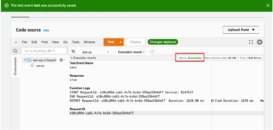
- Navigate to the Lambda console and choose the function. From the Test dropdown, choose Configure Test Event.

- Choose Create a new Test Event and select the template for the service you want to act as the trigger for your Lambda function. In this example, you choose Amazon DynamoDB Update.

- Save the test event and choose Test in the Code source section. Each user can create up to 10 test events per function. Those test events are private to you. Lambda runs the function on your behalf. The function handler receives and then processes the sample event.

- The Execution result shows the execution status as succeeded.


End-to-end testing
When testing your serverless applications end-to-end, it’s important to understand your user and data flows. The most important business-critical flows of your software are what should be tested end-to-end in your UI.
From a business perspective, these should be the most valuable user and data flows that occur in your product. Another resource to utilize is data from your customers. From your analytics platform, find the actions that users are doing the most in production.
End-to-end tests should be running in your build pipeline and act as blockers if one of them fails. They should also be updated as new features are added to your product.
The testing pyramid

The standard testing pyramid above on the left indicates that systems should have more unit tests than any other type of test, then a medium number of integration tests, and the least number of end-to-end tests.
However, when testing serverless applications, this standard shifts to a hexagonal structure on the right because it’s mostly made up of two or more AWS services talking to each other. You can mock out those integrations with tools such as moto or localstack.
Add automated tests to your CI/CD pipeline
As serverless applications scale, having automated tests is essential in getting fast feedback on the current state of your product. It is not scalable to test everything manually, so investing in an automation tool to run your tests is essential.
All of the tests in your build pipeline, including unit, integration, and end-to-end tests should be blocking in your CI/CD pipeline. This means if one of them fails, it should block the promotion of that code into production. And remember – there’s no such thing as a flakey test. Either the test does what it’s supposed to do, or it doesn’t.
Narrowly scope your tests
Testing asynchronous processes can be tricky. Not only must you monitor different parts of your system, you also need to know when to stop waiting and end the test. When there are multiple asynchronous steps, the delays add up to a longer-running test. It’s also more difficult to estimate how long we should wait before ending. There are two approaches to mitigate these issues.
Firstly, write separate, more narrowly-scoped tests over each asynchronous step. This limits the possible causes of asynchronous test failure you need to investigate. Also, with fewer asynchronous steps, these tests will run quicker and it will be easier to estimate how long to wait before timing out.
Secondly, verify as much of your system as possible using synchronous tests. Then, you only need asynchronous tests to verify residual concerns that aren’t already covered. Synchronous tests are also easier to diagnose when they fail, so you want to catch as many issues with them as possible before running your asynchronous tests.
Conclusion
In this blog post, you learn the three types of testing – unit testing, integration testing, and end-to-end testing. Then you learn how to configure test events with Lambda. I then cover the shift from the standard testing pyramid to the hexagonal testing pyramid for serverless, and why more integration tests are necessary. Then you learn a few best practices to keep in mind for getting started with testing your serverless applications.
For more information on serverless, head to Serverless Land.
What to Consider when Selecting a Region for your Workloads
Post Syndicated from Saud Albazei original https://aws.amazon.com/blogs/architecture/what-to-consider-when-selecting-a-region-for-your-workloads/
The AWS Cloud is an ever-growing network of Regions and points of presence (PoP), with a global network infrastructure that connects them together. With such a vast selection of Regions, costs, and services available, it can be challenging for startups to select the optimal Region for a workload. This decision must be made carefully, as it has a major impact on compliance, cost, performance, and services available for your workloads.
Evaluating Regions for deployment
There are four main factors that play into evaluating each AWS Region for a workload deployment:
- Compliance. If your workload contains data that is bound by local regulations, then selecting the Region that complies with the regulation overrides other evaluation factors. This applies to workloads that are bound by data residency laws where choosing an AWS Region located in that country is mandatory.
- Latency. A major factor to consider for user experience is latency. Reduced network latency can make substantial impact on enhancing the user experience. Choosing an AWS Region with close proximity to your user base location can achieve lower network latency. It can also increase communication quality, given that network packets have fewer exchange points to travel through.
- Cost. AWS services are priced differently from one Region to another. Some Regions have lower cost than others, which can result in a cost reduction for the same deployment.
- Services and features. Newer services and features are deployed to Regions gradually. Although all AWS Regions have the same service level agreement (SLA), some larger Regions are usually first to offer newer services, features, and software releases. Smaller Regions may not get these services or features in time for you to use them to support your workload.
Evaluating all these factors can make coming to a decision complicated. This is where your priorities as a business should influence the decision.
Assess potential Regions for the right option
Evaluate by shortlisting potential Regions.
- Check if these Regions are compliant and have the services and features you need to run your workload using the AWS Regional Services website.
- Check feature availability of each service and versions available, if your workload has specific requirements.
- Calculate the cost of the workload on each Region using the AWS Pricing Calculator.
- Test the network latency between your user base location and each AWS Region.
At this point, you should have a list of AWS Regions with varying cost and network latency that looks something Table 1:
| Region | Compliance | Latency | Cost | Services / Features |
|---|---|---|---|---|
| Region A |
✓ |
15 ms | $$ | ✓ |
| Region B |
✓ |
20 ms |
$$$ |
X |
| Region C |
✓ |
80 ms | $ |
✓ |
Table 1. Region evaluation matrix
Many workloads such as high performance computing (HPC), analytics, and machine learning (ML), are not directly linked to a customer-facing application. These would not be sensitive to network latency, so you may want to select the Region with the lowest cost.
Alternatively, you may have a backend service for a game or mobile application in which network latency has a direct impact on user experience. Measure the difference in network latency between each Region, and determine if it is worth the increased cost. You can leverage the Amazon CloudFront edge network, which helps reduce latency and increases communication quality. This is because it uses a fully managed AWS network infrastructure, which connects your application to the edge location nearest to your users.
Multi-Region deployment
You can also split the workload across multiple Regions. The same workload may have some components that are sensitive to network latency and some that are not. You may determine you can benefit from both lower network latency and reduced cost at the same time. Here’s an example:

Figure 1. Multi-Region deployment optimized for feature availability
Figure 1 shows a serverless application deployed at the Bahrain Region (me-south-1) which has a close proximity to the customer base in Riyadh, Saudi Arabia. Application users enjoy a lower latency network connecting to the AWS Cloud. Analytics workloads are deployed in the Ireland Region (eu-west-1), which has a lower cost for Amazon Redshift and other features.
Note that data transfer between Regions is not free and, in this example, costs $0.115 per GB. However, even with this additional cost factored in, running the analytical workload in Ireland (eu-west-1) is still more cost-effective. You can also benefit from additional capabilities and features that may have not yet been released in the Bahrain (me-south-1) Region.
This multi-Region setup could also be beneficial for applications with a global user base. The application can be deployed in multiple secondary AWS Regions closer to the user base locations. It uses a primary AWS Region with a lower cost for consolidated services and latency-insensitive workloads.

Figure 2. Multi-Region deployment optimized for network latency
Figure 2 allows for an application to span multiple Regions to serve read requests with the lowest network latency possible. Each client will be routed to the nearest AWS Region. For read requests, an Amazon Route 53 latency routing policy will be used. For write requests, an endpoint routed to the primary Region will be used. This primary endpoint can also have periodic health checks to failover to a secondary Region for disaster recovery (DR).
Other factors may also apply for certain applications such as ones that require Amazon EC2 Spot Instances. Regions differ in size, with some having three, and others up to six Availability Zones (AZ). This results in varying Spot Instance capacity available for Amazon EC2. Choosing larger Regions offers larger Spot capacity. A multi-Region deployment offers the most Spot capacity.
Conclusion
Selecting the optimal AWS Region is an important first step when deploying new workloads. There are many other scenarios in which splitting the workload across multiple AWS Regions can result in a better user experience and cost reduction. The four factors mentioned in this blog post can be evaluated together to find the most appropriate Region to deploy your workloads.
If the workload is bound by any regulations, shortlist the Regions that are compliant. Measure the network latency between each Region and the location of the user base. Estimate the workload cost for each Region. Check that the shortlisted Regions have the services and features your workload requires. And finally, determine if your workload can benefit from running in multiple Regions.
Dive deeper into the AWS Global Infrastructure Website for more information.
[$] More Rust concepts for the kernel
Post Syndicated from original https://lwn.net/Articles/869428/rss
The first day of the Kangrejos (Rust for Linux) conference
introduced the project and what it was trying to accomplish; day 2 covered a number of core Rust
concepts and their relevance to the kernel. On the third and final day of
the conference, Wedson Almeida Filho delved deeper into how Rust can be
made to work in the Linux kernel, covered some of the lessons that have been
learned so far, and discussed next steps with a number of kernel
developers.
Kim Scott | Just Work | Talks at Google
Post Syndicated from Talks at Google original https://www.youtube.com/watch?v=HenYIyjR740