In a recent evaluation of AI models’ cyber capabilities, current Claude models can now succeed at multistage attacks on networks with dozens of hosts using only standard, open-source tools, instead of the custom tools needed by previous generations. This illustrates how barriers to the use of AI in relatively autonomous cyber workflows are rapidly coming down, and highlights the importance of security fundamentals like promptly patching known vulnerabilities.
[…]
A notable development during the testing of Claude Sonnet 4.5 is that the model can now succeed on a minority of the networks without the custom cyber toolkit needed by previous generations. In particular, Sonnet 4.5 can now exfiltrate all of the (simulated) personal information in a high-fidelity simulation of the Equifax data breach—one of the costliest cyber attacks in history—using only a Bash shell on a widely-available Kali Linux host (standard, open-source tools for penetration testing; not a custom toolkit). Sonnet 4.5 accomplishes this by instantly recognizing a publicized CVE and writing code to exploit it without needing to look it up or iterate on it. Recalling that the original Equifax breach happened by exploiting a publicized CVE that had not yet been patched, the prospect of highly competent and fast AI agents leveraging this approach underscores the pressing need for security best practices like prompt updates and patches.
Read the whole thing. Automatic exploitation will be a major change in cybersecurity. And things are happening fast. There have been significant developments since I wrote this in October.
As organizations scale their observability and analytics capabilities across multiple AWS Regions and environments, maintaining consistent dashboards becomes increasingly complex. Teams often spend hours manually recreating dashboards, creating workspaces, linking data sources, and validating configurations across deployments—a repetitive and error-prone process that slows down operational visibility.
The next generation OpenSearch UI in Amazon OpenSearch Service introduces a unified, managed analytics experience that decouples from individual OpenSearch domains and OpenSearch collections. It provides workspaces, dedicated team spaces with collaborator management and a tailored environment for observability, search, and security analytics use cases. Each workspace can connect to multiple data sources, including OpenSearch Service domains, Amazon OpenSearch Serverless collections, and external sources such as Amazon Simple Storage Service (Amazon S3). OpenSearch UI also supports access with AWS IAM Identity Center, AWS Identity and Access Management (IAM), Identity provider (IdP)-initiated single sign-on (SAML using IAM federation), and AI-powered insights.)-initiated single sign-on (SAML using IAM federation),and AI-powered insights.
In this post, you’ll learn how to use the AWS Cloud Development Kit (AWS CDK) to deploy an OpenSearch UI application and integrate it with an AWS Lambda function that automatically creates workspaces and dashboards using the OpenSearch Dashboards Saved Objects APIs. Using this automation means that environments launch with ready-to-use analytics that are standardized, version-controlled, and consistent across deployments. that are standardized, version-controlled, and consistent across deployments.
Specifically, you’ll learn how to:
Deploy an OpenSearch UI application using AWS CDK that in turn uses AWS CloudFormation
Automatically create workspaces and dashboards using a Lambda based custom resource
Generate and ingest sample data for immediate visualization
Build visualizations programmatically using the OpenSearch Dashboards Saved Objects API
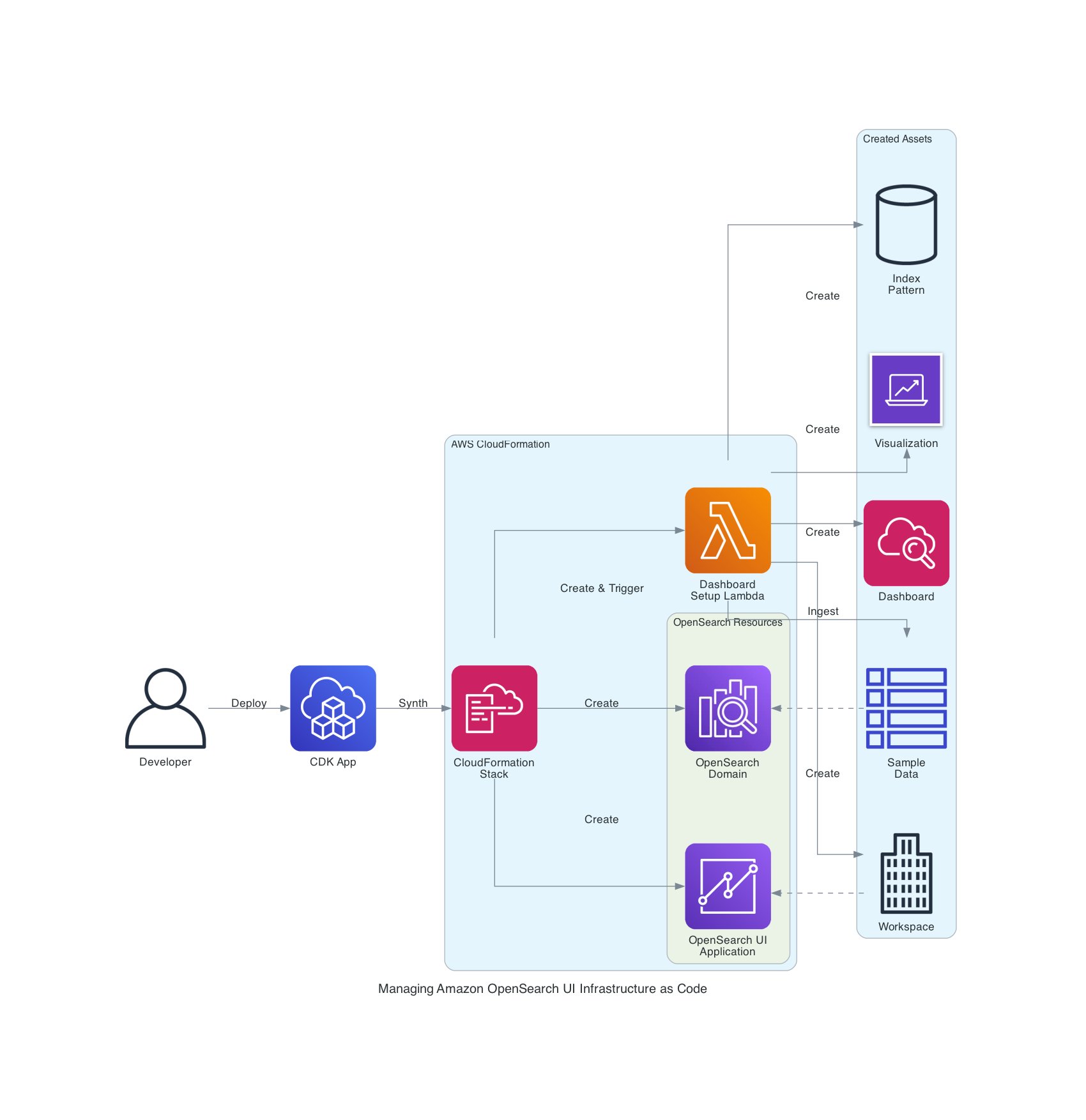
The following architecture demonstrates how to automate OpenSearch UI workspace and dashboard creation using AWS CDK, AWS Lambda, and the OpenSearch UI APIs.
The workflow flows from left to right:
Deploy stack – Developer runs cdk deploy to launch the infrastructure and create the CloudFormation stack.
Create domain – CloudFormation creates the OpenSearch domain (which serves as the data source)
Trigger Lambda – CloudFormation invokes the Lambda function as a custom resource
Generate and ingest data – Lambda generates sample metrics and ingests them into the domain
Create workspaces and assets using saved object API – Lambda creates the workspace, index pattern, visualization (pie chart), and dashboard using OpenSearch UI API calls
The result is a fully configured OpenSearch UI with sample data and a ready-to-use dashboard automated through infrastructure as code (IaC). The same workflow can also be integrated into existing infrastructure for OpenSearch UI applications to automatically create or update dashboards during future deployments, maintaining consistency across environments. consistency across environments.
Prerequisites
To perform the solution, you need the following prerequisites:
An AWS user or role with sufficient permissions – You’ll need permissions to create and manage AWS resources such as OpenSearch Service domains, OpenSearch UI applications, Lambda functions, IAM roles and policies, virtual private cloud (VPC) networking components (subnets and security groups), and CloudFormation stacks. For testing or proof-of-concept deployments, we recommend using an administrative role. For production, follow the principle of least privilege.
This sample demonstrates how to deploy an OpenSearch UI application, create a workspace, ingest sample data, and automatically generate visualizations and dashboards using IaC.
After cloning the repository, you can deploy the stack to automatically create your first OpenSearch workspace and dashboard with sample data.
Understanding the solution
Before deploying, let’s examine how the solution works. The following steps explain the architecture and automation logic that will execute automatically when you deploy the AWS CDK stack. The next section contains the actual deployment commands you’ll run.
Provision OpenSearch UI resources
The AWS CDK integrates seamlessly with AWS CloudFormation. This means you can define your OpenSearch resources and automation workflows as IaC. In this solution, AWS CDK provisions the OpenSearch domain, OpenSearch UI application, and a Lambda based custom resource that performs the automation logic.
When deploying OpenSearch UI automation, the order of resource creation is important to correctly resolve dependencies. The recommended order is as follows:
Create the Lambda execution role – Required for access to AppConfigs and APIs
Create the OpenSearch domain – Serves as the primary data source
Create the OpenSearch UI application – References the Lambda role in its AppConfigs
Create the Lambda function – Defines the automation logic
Create the custom resource – Triggers the Lambda automation during stack deployment
The following code snippet (from cdk/lib/dashboard-stack.ts) shows the key infrastructure definitions:
The Lambda role must be created before the OpenSearch UI application so its Amazon Resource Name (ARN) can be referenced in dashboardAdmin.groups
The Lambda role includes both opensearch:ApplicationAccessAll (for OpenSearch UI API access) and es:ESHttp* permissions (for ingesting data into the OpenSearch domain)
The custom resource enables the automation function to run during deployment, passing both OpenSearch UI and OpenSearch domain endpoints as parameters
Authenticate with OpenSearch UI APIs
When programmatically interacting with the OpenSearch UI (Dashboards) APIs, proper authentication is required so your Lambda function or automation script can securely access the APIs. The OpenSearch UI uses AWS Signature Version 4 (SigV4) authentication—similar to the OpenSearch domain APIs—but with a few important distinctions.
When signing OpenSearch UI API requests, the service name must be opensearch, not es. This is a common source of confusion: the OpenSearch domain endpoint still uses the legacy service name es, but the OpenSearch UI endpoints require opensearch. Using the wrong service name will cause your requests to fail authentication, even if the credentials are valid.
For POST, PUT, or DELETE requests, include the following headers to satisfy the OpenSearch UI API security requirements:
Header
Description
1
Content-Type
Set to application/json for JSON payloads
2
osd-xsrf
Required for state-changing operations (set to true)
3
x-amz-content-sha256
SHA-256 hash of the request body to ensure data integrity
The SigV4 signing process automatically computes this body hash when using the botocore AWSRequest object, maintaining request integrity and preventing tampering during transmission.
The following code snippet (from lambda/sigv4_signer.py) demonstrates how to sign and send a request to the OpenSearch UI API:
def get_common_headers(body: bytes = b"{}") -> Dict[str, str]:
    """
    Get common headers for OpenSearch UI API requests.

    Args:
        body: Request body bytes to hash

    Returns:
        Dictionary of required headers
    """
    body_hash = hashlib.sha256(body).hexdigest()
    return {
        "Content-Type": "application/json",
        "x-amz-content-sha256": body_hash,
        "osd-xsrf": "osd-fetch",
        "osd-version": "3.1.0",
    }


def make_signed_request(
    method: str,
    url: str,
    headers: Dict[str, str],
    body: bytes = b"",
    region: str = None,
) -> Any:
    session = boto3.Session()
    if not region:
        region = session.region_name

    # Create AWS request
    request = AWSRequest(method=method, url=url, data=body, headers=headers)

    # Sign with SigV4 using 'opensearch' service name (not 'es')
    credentials = session.get_credentials()
    SigV4Auth(credentials, "opensearch", region).add_auth(request)

    # Send request using URLLib3Session
    http_session = URLLib3Session()
    return http_session.send(request.prepare())
This utility function signs the request using the correct service name (opensearch), attaches the required headers, and sends it securely to the OpenSearch UI endpoint.
Create workspace and dashboard with sample data
The Lambda function (lambda/dashboard_automation.py) automates the entire process of provisioning a workspace, generating sample data, and creating visualizations and dashboards through the OpenSearch UI APIs. Visit the following lists of APIs:
Locate or create a workspace. Each dashboard in the OpenSearch UI must exist within a workspace. The function first checks whether a workspace already exists and creates one if necessary. The workspace associates one or more data sources (for example, an OpenSearch domain or OpenSearch Serverless collection):
This logic enables repeated deployments to remain idempotent; the Lambda function reuses existing workspaces rather than creating duplicates.
Generate and ingest sample data. To make the dashboards meaningful upon first launch, the Lambda function generates a small dataset simulating HTTP request metrics and ingests it into the OpenSearch domain using the Bulk API:
def generate_sample_metrics(num_docs: int = 50) -> list:
    """Generate realistic HTTP API request metrics."""
    endpoints = ["/api/users", "/api/products", "/api/orders"]
    status_codes = [200, 201, 400, 404, 500]
    status_weights = [0.70, 0.15, 0.08, 0.05, 0.02]  # Realistic distribution

    documents = []
    for i in range(num_docs):
        documents.append({
            "@timestamp": generate_timestamp(),
            "endpoint": random.choice(endpoints),
            "status_code": random.choices(status_codes, weights=status_weights)[0],
            "response_time_ms": random.randint(20, 500)
        })
    return documents
The function then ingests this data into the domain:
This enables each deployment to include sample analytics data that immediately populates the dashboard upon first login.
Create a visualization. After the index pattern is available, the Lambda function creates a pie chart visualization that shows HTTP status code distribution:
This completes the dashboard creation process, providing users with an interactive visualization of application metrics as soon as they access the workspace.
The full implementation, including logging, error handling, and helper utilities, is available in the AWS Samples GitHub repository.
Deploy the infrastructure with AWS CDK
With the AWS CDK stack and Lambda automation in place, you’re ready to deploy the full solution and verify that your OpenSearch UI dashboard is created automatically.
Deploy the stack
From the root directory of the cloned repository, navigate to the AWS CDK folder and deploy the stack using your IAM user ARN from the Prerequisites section:
cd cdk
npm install
npx cdk bootstrap  # First time only
npx cdk deploy -c masterUserArn=arn:aws:iam::123456789012:user/your-username
The deployment process typically takes 20–25 minutes because AWS CDK provisions the OpenSearch domain, OpenSearch UI application, Lambda function, and custom resource that runs the automation.
Verify the deployment
After the deployment completes:
Open the OpenSearch UI endpoint displayed in the AWS CDK output.
Sign in using your IAM credentials.
Switch to the newly created workspace-demo workspace.
Open the Application Metrics dashboard.
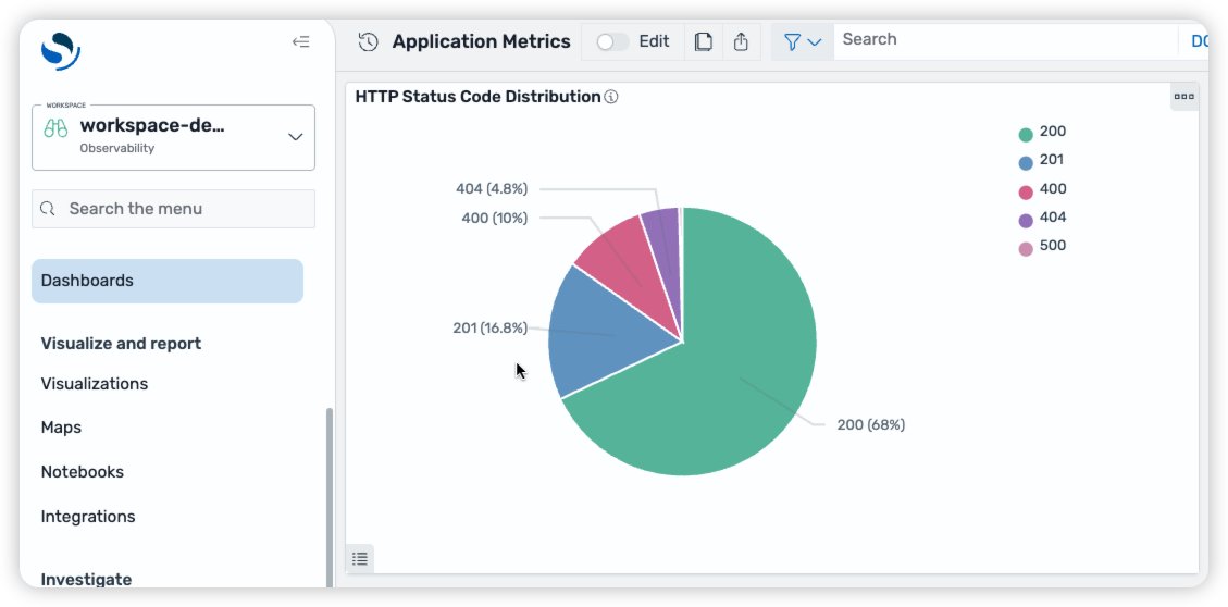
View the pie chart visualization that displays the distribution of HTTP status codes from the sample data.
The dashboard automatically displays a pie chart visualization populated with synthetic application metrics, demonstrating how the Saved Objects API can be used to bootstrap meaningful analytics dashboards immediately after deployment.
Enhancement 1: Simplify dashboard creation with Saved Object Import API
As your OpenSearch Dashboards evolve, managing complex dependencies between index patterns, visualizations, and dashboards can become increasingly difficult. Each dashboard often references multiple saved objects, and manually recreating or syncing them across environments can be time-consuming and error prone.
To simplify this process, we recommend using the Saved Objects Import/Export API. You can use this API to bundle entire dashboards, including their dependent objects, into a single transferable artifact. By using this approach, you can version, migrate, and deploy dashboards across environments as part of your CI/CD workflow, maintaining consistency and reducing operational overhead.
Select the dashboard and related objects (for example, visualizations and index patterns)
Choose Export
Save the exported file as dashboard.ndjson
This file contains saved objects serialized in newline-delimited JSON (NDJSON) format, ready for versioning or deployment automation.
Import dashboards programmatically
You can programmatically import the NDJSON file into a target workspace using the Saved Objects import API:
# Pseudo code for import function
def import_dashboard(workspace_id, ndjson_file):
    # Read the exported dashboard file
    dashboard_config = read_file(ndjson_file)


    # POST to import to opensearch ui endpoint
    url = f"{opensearch_ui_endpoint}/w/{workspace_id}/api/saved_objects/_import"
    response = make_signed_request("POST", url, dashboard_config)

    return response.success
By using this approach, you can treat dashboards as deployable assets, exactly like application code. You can store your exported dashboards in source control, integrate them into your AWS CDK or CloudFormation pipelines, and automatically deploy them to multiple environments with confidence.
Enhancement 2: Improved security configurations
In some cases, you might want to improve the security configuration of your OpenSearch UI application, or you might be dealing with OpenSearch domains that have been deployed with additional security configurations. In this section, we discuss how you can improve the security configuration of your OpenSearch UI application and still achieve IaC with AWS CDK. More specifically, we explain how you can set up your OpenSearch UI application when your OpenSearch domain is in a VPC and when fine-grained access control is enabled.
When the OpenSearch Domain resides within a VPC, additional configurations will be needed to properly connect with your dashboard.
Enable communication between Lambda functions used to ingest data and the OpenSearch domain in the VPC
When the OpenSearch Service domain resides in a VPC, the Lambda functions that ingest data into the domain must be able to communicate with it. The most straightforward way of doing this is to allow the Lambda function to be executed within the same VPC as your OpenSearch Service domain and give it the same security group. An example is provided in the GitHub repository.
Allow HTTPS communications from clients trying to communicate with your OpenSearch Service domain. In this example, the client will be using the same security group used in the OpenSearch Service domain:
openSearchSecurityGroup.addIngressRule(
  openSearchSecurityGroup,
  ec2.Port.tcp(443),
  'Allow inbound HTTPS traffic from itself',
);
Add this managed policy to the role assumed by the Lambda function to allow it access to the VPC:
Specify the VPC and the security group your Lambda function will be using. In this case, the VPC is the same one used by your OpenSearch Service domain:
Authorize OpenSearch UI service for VPC endpoint access
For the OpenSearch Service domain to be accessible to your dashboard, VPC endpoint access must be enabled. This can be achieved by using a custom resource, as shown in the following configuration:
When you use fine-grained access control in combination with an OpenSearch UI, you have more control over which operations are allowed for each user. This can be especially useful when you want to limit your users’ actions beyond the admin, read, or write permissions that come with OpenSearch UI. Unique roles can be created and mapped to one or more users to achieve precise control over who can access what functionality.
In the previous sections, the same Lambda was used to make requests to both the OpenSearch Service domain and the OpenSearch UI. However, in situations where the main role isn’t the same between the OpenSearch Service domain and the OpenSearch UI, we recommend creating a Lambda function for each role. Again, when deploying OpenSearch UI automation, the order of resource creation is important to correctly resolve dependencies. As illustrated previously, the recommended order is as follows:
Create the dashboard Lambda execution role – Required for access to AppConfigs and APIs
Create the OpenSearch domain main role – Required for domain creation and APIs
Create the OpenSearch domain – Serves as the primary data source
Create the OpenSearch domain Lambda function – Defines the automation logic for the OpenSearch domain
Create the OpenSearch domain custom resources – Triggers the Lambda automation during stack deployment
Create the OpenSearch UI application – References the Lambda role in its AppConfigs
Create the OpenSearch UI Lambda function – Defines the automation logic for the OpenSearch UI
Create the OpenSearch UI custom resource – Triggers the Lambda automation during stack deployment
When creating the OpenSearch Service domain, specify the fine-grained access control parameter, as follows:
// Step 3: Create OpenSearch Domain
const opensearchDomain = new opensearch.Domain(this, 'OpenSearchDomain', {
  // ... additional configuration
  // Enable Fine-Grained Access Control in your OpenSearch Domain
  fineGrainedAccessControl: {
    masterUserArn: openSearchMasterRole.roleArn,
  }
});
The Lambda function responsible for communicating with the OpenSearch Service domain should have the necessary permissions to write to it. The following is a configuration example where the Lambda function assumes the domain’s main role:
// Step 4: Create Lambda Function for OpenSearch Domain
const domainFn = new lambda.Function(this, 'DomainSetup', {
  // ... additional configuration
  role: openSearchMasterRole
});
Then, add the custom resources to create the roles and role mappings, as needed:
// Step 5: Create Custom Resources for OpenSearch Domain
const domainProvider = new cr.Provider(this, 'DomainProvider', {
  onEventHandler: domainFn
});

// A custom resource to create roles (Optional)
new cdk.CustomResource(this, 'DomainRoleSetupResource', {
  serviceToken: domainProvider.serviceToken,
  // ... additional configuration
});

// A custom resource to create role mappings (Optional)
new cdk.CustomResource(this, 'DomainRolesMappingSetupResource', {
  serviceToken: domainProvider.serviceToken,
  // ... additional configuration
});
Create additional roles in the OpenSearch Service domain (Optional)
If you want to grant specific permissions to some users, we recommend creating roles for them. This can be achieved by making the following requests to the OpenSearch Service domain endpoint.
For more information about the roles endpoint, review the Create role in the OpenSearch documentation.
Create role mappings in the OpenSearch domain for your dashboard users (Optional)
Users can be mapped to one or more roles to control their access to the OpenSearch Service domain, which will be reflected in the OpenSearch UI dashboard connected to the domain.
For more information about the rolesmapping endpoint, review the Create role mapping in the OpenSearch documentation.
# Pseudo code to create a role mapping
def create_role_mapping(domain_endpoint: str, region: str,
                        new_role_name: str) -> bool:
    """Create a new role mapping"""
    url = f"https://{domain_endpoint}/_plugins/_security/api/rolesmapping/{new_role_name}"

    payload = {
        "backend_roles": [
            "<ROLE_ARN_1>",
            "<ROLE_ARN_2>",
        ],
    }

    response = make_domain_request("PUT", url, headers, json.dumps(payload).encode(), region)
    return response.success
These are some important implementation notes:
By default, the OpenSearch Domain will create a role mapping for its main user, under all_access and security_manager. If you modify those mappings, we recommend keeping the main user in the list to prevent accidental loss of access.
When fine-grained access control is used, if a user opens the OpenSearch UI without being mapped to a role in the OpenSearch Domain, they will be unable to visualize or modify the data located in the OpenSearch Domain, even if they’re part of the OpenSearch UI’s admin group. For this reason, we recommend creating custom resources to add the appropriate role mappings. OpenSearch UI admins will still be able to make changes to the OpenSearch UI dashboards.
When programmatically interacting with the OpenSearch Domain APIs, proper authentication is required so your Lambda function or automation script can securely access the APIs. The OpenSearch Domain uses SigV4 authentication. When signing the OpenSearch Domain API requests, the service name must be es.
Cost considerations
This solution uses several AWS services, each with its own cost component:
Amazon OpenSearch Service – This is the main cost driver. Charges are based on instance type, number of nodes, and Amazon Elastic Block Store (Amazon EBS) storage. For testing, you can use a smaller instance (for example, t3.small.search) or delete the domain after use to minimize cost.) or delete the domain after use to minimize cost.
AWS Lambda – The automation function runs only during deployment and incurs minimal charges for a few short invocations.
AWS CDK and CloudFormation – Create temporary IAM roles and Amazon S3 deployment assets with negligible cost.
To avoid incurring ongoing costs, clean up the resources created by this solution when you’ve completed your testing.Open your project directory and destroy the AWS CDK stack:
cd cdk
npx cdk destroy
This command removes the resources provisioned by the AWS CDK stack, including:
The Amazon OpenSearch Service domain
The OpenSearch UI application
The AWS Lambda function and custom resource
IAM roles and policies associated with the deployment
By cleaning up, you stop the related charges and maintain a tidy, cost-efficient AWS environment.
By integrating the Saved Objects API with the next-generation Amazon OpenSearch UI, you can programmatically create entire analytics experiences—including workspaces, sample data, visualizations, and dashboards—directly from your IaC.
This approach brings the power of IaC to your analytics layer. Using AWS CDK and AWS Lambda, you can version, deploy, and update dashboards consistently across environments, reducing manual setup while improving reliability and governance. With this automation in place, your teams can focus on insights rather than setup—delivering observability-as-code that scales with your organization.
The
Linux Kernel Runtime Guard (LKRG) is a out-of-tree loadable kernel module that
attempts to detect and report violations of the kernel’s internal invariants,
such as might be caused by an in-progress security exploit or a rootkit.
LKRG has been experimental since its
initial release in 2018. In September
2025, the project announced
the 1.0 version. With the promises of stability that version brings, users might want more
information to decide whether to include it in their kernel.
As generative AI has shifted from selective experimentation to broad operational use, large language models (LLMs) now sit inside developer environments, support workflows, internal knowledge systems, and security tooling itself. Adoption has widened for both enterprises and consumers alike, and, unsurprisingly, have a whole new set of security patterns.
Though oftentimes single catastrophic failures are the types of stories that make the news (like an AI agent pushing code to production against its explicit instructions), the truth is that there’s a bigger narrative here. Generative AI has introduced a whole new way to work, and we’re seeing a set of recurring behaviors—ways that AI systems interact with data, instructions, and people—that either introduce new risks or enhance some tried-and-true bad actor tactics (like more convincing phishing attacks, for example).
This article focuses on seven patterns that have emerged in real deployments and documented incidents. Let’s get into it.
1. Prompt injection and instruction hijacking
Prompt injection has matured from a research concept into a practical exploit vector. The issue is structural: LLMs interpret text holistically using tokenization, which makes it difficult to maintain a strict separation between instructions and data. When untrusted content is introduced into an AI system with elevated permissions, that ambiguity becomes exploitable.
Recent incidents show how this plays out in production tools. Researchers analyzing Microsoft Copilot demonstrated that carefully crafted inputs could override intended behavior, expose system prompts, or trigger unintended actions within the model’s sandbox.
The common thread is authority. When models are allowed to act on retrieved content or invoke downstream tools, text becomes a control surface.
2. Prompt poaching and peripheral exfiltration
Not all AI-related data loss requires access to the model itself. A recent malware campaign demonstrated how attackers can siphon AI conversations by compromising the surrounding ecosystem.
These attacks target trust boundaries adjacent to AI systems rather than the models directly. Browser extensions, plugins, and integrations become collection points for high-value contextual data that did not previously exist in a single place. And, they’re often less controlled by enterprise IT teams compared with other types of software.
3. AI-powered malware and ransomware
AI-assisted malware is no longer hypothetical. Security researchers have now documented ransomware that uses generative models as part of its operational logic.
One example: PromptLock, a ransomware strain that leverages LLMs to dynamically generate portions of its code and behavior during execution.
At the ecosystem level, threat intelligence reports show ransomware groups using AI to accelerate development, customize payloads, and craft tailored extortion communications. Akamai’s 2025 ransomware trends report documents LLM usage by active groups for both technical and social components of attacks.
It’s less about how it’s done and more about how fast it’s done: Iteration cycles are shorter, and adaptation happens more quickly.
4. Acceleration and competitive pressure in the ransomware economy
Even when AI is not embedded directly into malware, it influences the broader threat environment. Ransomware activity increased throughout 2025 despite arrests and takedowns; new groups emerged quickly to replace disrupted ones.
As we said above, speed matters here. Defensive models that assume time for analysis, tuning, and response are increasingly stressed by attackers who can prototype and redeploy faster than those cycles allow.
And it’s not just speed—the volume of (credible, real) attacks matters too. The truth of the game has always been that bad actors only have to succeed once whereas defenders have to succeed every time. If better ransomware is being produced more quickly, defenders are having to adapt just as (or more) quickly to a higher volume of attacks (which makes the demand for employees in the security industry that much more understandable).
5. Semantic noise and operational fatigue
Generative AI produces a large volume of plausible output: summaries, recommendations, alerts, explanations. In isolation, that capability is helpful; in aggregate, it introduces a new operational burden.
Security teams report growing difficulty distinguishing signal from well-formed noise. In reality, this means that over-taxed employees are getting pinged while on-call far more.
AI-generated conclusions often require human validation, but their tone and confidence can reduce scrutiny over time. That creates opportunities for malicious activity to hide inside outputs that appear reasonable and routine; or, on the flip side, for things like process and architecture misconfigurations to masquerade as security events by creating too many requests.
This pattern does not map cleanly to a single exploit; it shows up as delayed detection, slower response, and missed anomalies.
6. Code supply chain risk from generated code
AI-generated code compounds familiar supply-chain issues. Generated snippets often compile cleanly, pass tests, and follow common patterns; they also tend to replicate insecure defaults or omit contextual safeguards.
As these patterns are reused across services, small mistakes scale quickly. Not only that, but basic parameters like privileging recency (e.g., new security patches) vs. commonality (e.g., the most often used code) can have major implications and be weighted differently in different tools. While there is demonstrated risk of malicious insertion, it’s also the normalization of fragile or incomplete logic through automation.
7. Potential human skill erosion as a force multiplier
One of the quietest risks is also the hardest to measure. As AI tools handle more analysis, summarization, and decision support, human operators spend less time interrogating raw data. That’s both a good and a bad thing—really, it begs the question of how we go about creating and applying expertise in a new and developing epistemological framework. (Wait, you thought engineering wasn’t philosophical?)
Over time, that shifts how teams validate outcomes and how comfortable they are challenging AI-generated conclusions. This erosion does not cause incidents by itself, but it can amplify the impact of every other failure mode.
Where this leaves us
Across these examples, a consistent theme emerges. Generative AI changes how authority, context, and action flow through systems. Many of the resulting failures are subtle and blend into normal usage patterns.
The next phase of response is already taking shape. Government agencies and standards bodies are beginning to formalize guidance on securing AI systems, managing AI-related risk, and adapting existing security practices to these new patterns.
That guidance belongs in its own discussion. For now, the takeaway is simpler: AI adoption has altered the shape of risk.
In this post, we show how to migrate an Oracle data warehouse to Amazon Redshift using Oracle GoldenGate and DMS Schema Conversion, a feature of AWS Database Migration Service (AWS DMS). This approach facilitates minimal business disruption through continuous replication. Amazon Redshift is a fast, fully managed, petabyte-scale data warehouse service that makes it simple and cost-effective to efficiently analyze your data using your existing business intelligence tools.
Solution overview
Our migration approach combines DMS Schema Conversion for schema migration and Oracle GoldenGate for data replication. The migration process consists of four main steps:
Schema conversion using DMS Schema Conversion.
Initial data load using Oracle GoldenGate.
Change data capture (CDC) for ongoing replication.
Final cutover to Amazon Redshift.
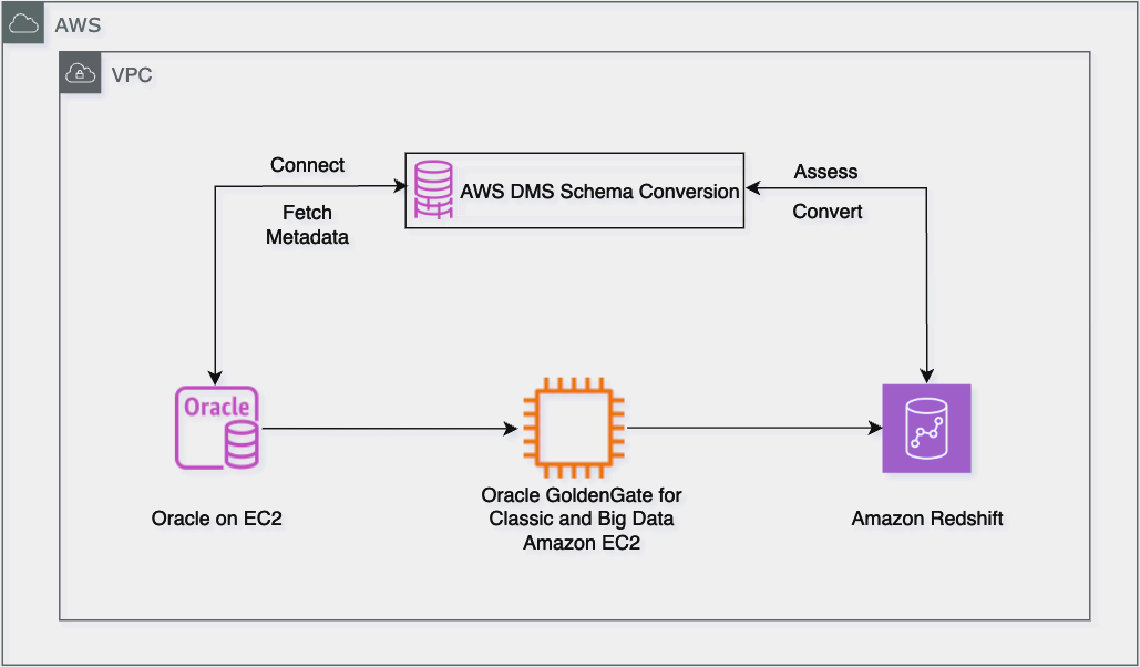
The following diagram shows the migration workflow architecture from Oracle to Amazon Redshift, where DMS Schema Conversion handles schema migration and Oracle GoldenGate manages both initial data load and continuous replication through Extract and Replicat processes running on Amazon Elastic Compute Cloud (Amazon EC2) instances. The solution facilitates minimal downtime by maintaining real-time data synchronization until the final cutover.
The solution comprises the following key migration components:
In the following sections, we walk through how to migrate an Oracle data warehouse to Amazon Redshift. For demonstration purposes, we use an Oracle data warehouse consisting of four tables:
DMS Schema Conversion automatically converts your Oracle database schemas and code objects to Amazon Redshift-compatible formats. This includes tables, views, stored procedures, functions, and data types.
Set up network for DMS Schema Conversion
DMS Schema Conversion requires network connectivity to both your source and target databases. To set up this connectivity, complete the following steps:
Specify a virtual private cloud (VPC) and subnet where DMS Schema Conversion will run.
Configure security group rules to allow traffic between the following:
DMS Schema Conversion and your source Oracle database
DMS Schema Conversion and your target Redshift cluster
DMS Schema Conversion saves items such as assessment reports, converted SQL code, and information about database schema objects in an S3 bucket. For instructions to create an S3 bucket, refer to Create an S3 bucket.
Create IAM policies and roles
To set up DMS Schema Conversion, you must create appropriate IAM policies and roles. This process makes sure AWS DMS has the necessary permissions to access your source and target databases, as well as other AWS services required for the migration.
Prepare DMS Schema Conversion
In this section, we go through the steps to configure DMS Schema Conversion.
Set up instance profile
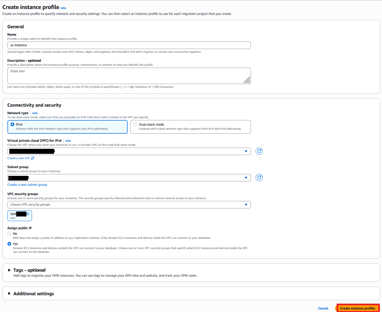
An instance profile specifies the network, security, and Amazon S3 settings for DMS Schema Conversion to use. Create an instance profile with the following steps:
On the AWS DMS console, choose Instance profiles in the navigation pane.
Choose Create instanceprofile.
For Name, enter a name (for example, sc-instance).
For Network type, we use IPv4. DMS Schema Conversion also offers Dual-stack mode for both IPv4 and IPv6.
For Virtual private cloud (VPC) for IPv4, choose Default VPC.
For Subnet group, choose your subnet group (for this post, default).
For VPC security groups, choose your security groups. As previously stated, the instance profile’s VPC security group must have access to both the source and target databases.
For S3 bucket, specify a bucket to store schema conversion metadata.
Choose Create instance profile.
Add data providers
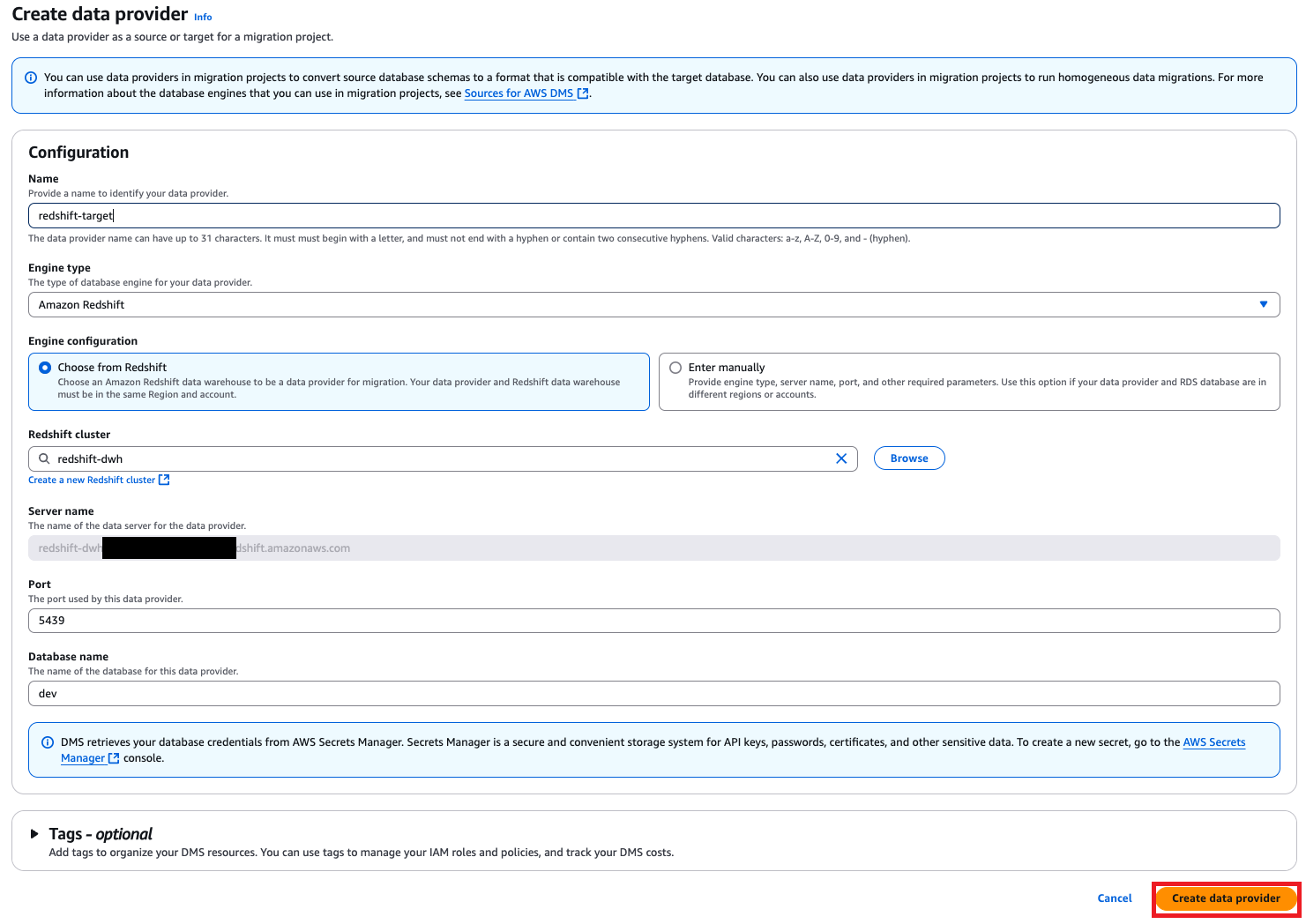
Data providers store database types and information about source and target databases for DMS Schema Conversion to connect to. Configure data providers for the source and target databases with the following steps:
On the AWS DMS console, choose Data providers in the navigation pane.
Choose Create data provider.
To create your target, for Name, enter a name (for example, redshift-target).
For Engine type, choose Amazon Redshift.
For Engine configuration, select Choose from Redshift.
For Redshift cluster, choose the target Redshift cluster.
For Port, enter the port number.
For Database name, enter the name of your database.
Choose Create data provider.
Repeat similar steps to create your source data provider.
Create migration project
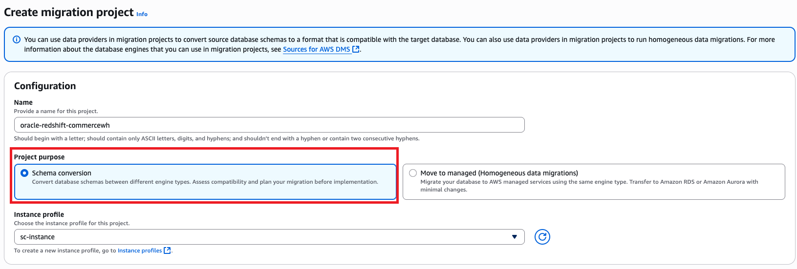
The DMS Schema Conversion migration project defines migration entities, including instance profiles, source and target data providers, and migration rules. Create a migration project with the following steps:
On the AWS DMS console, choose Migration projects in the navigation pane.
Choose Create migration project.
For Name, enter a name to identify your migration project (for example, oracle-redshift-commercewh).
For Instance profile, choose the instance profile you created.
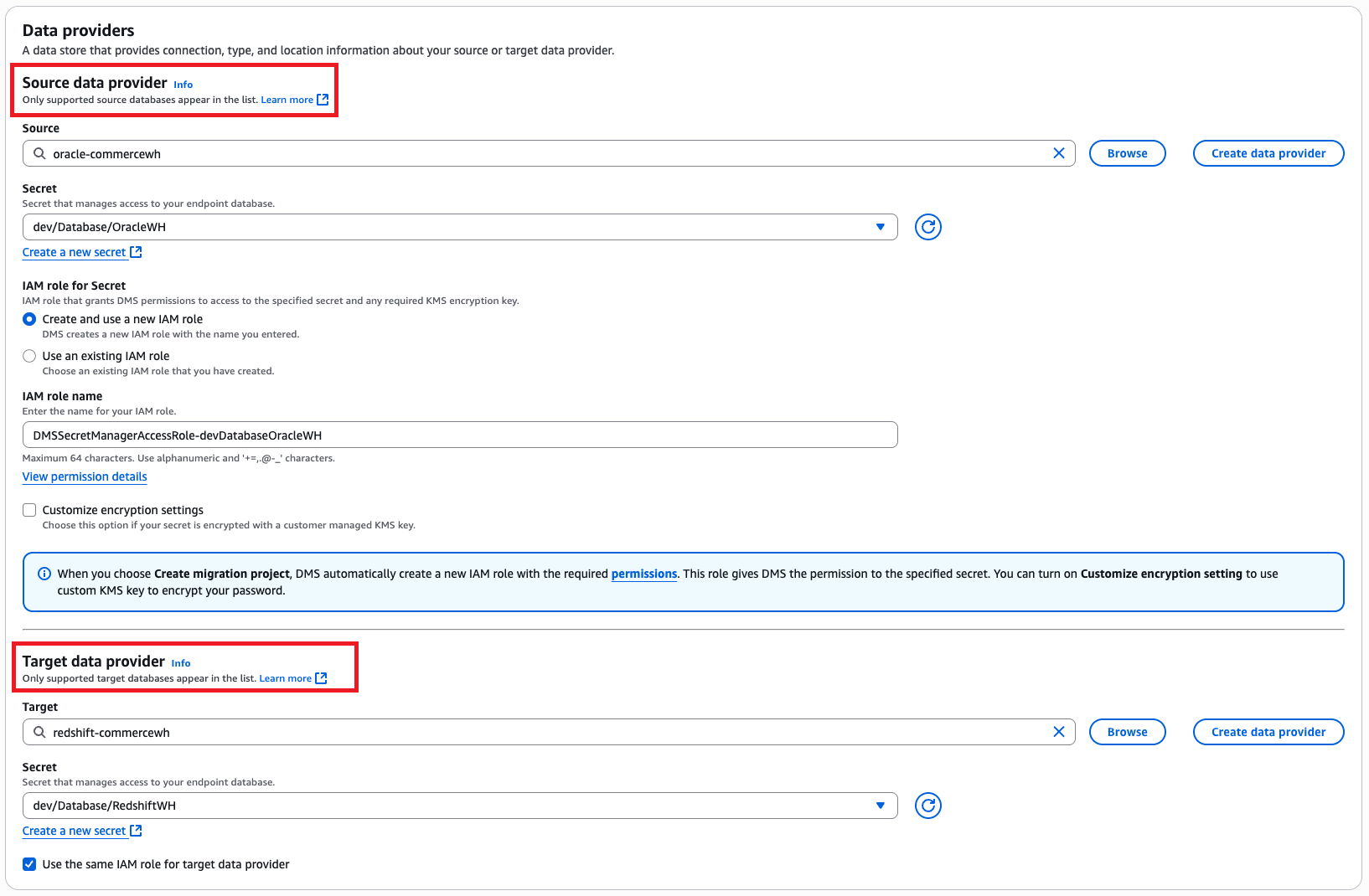
In the Data providers section, enter the source and target data providers, Secrets Manager secret, and IAM roles.
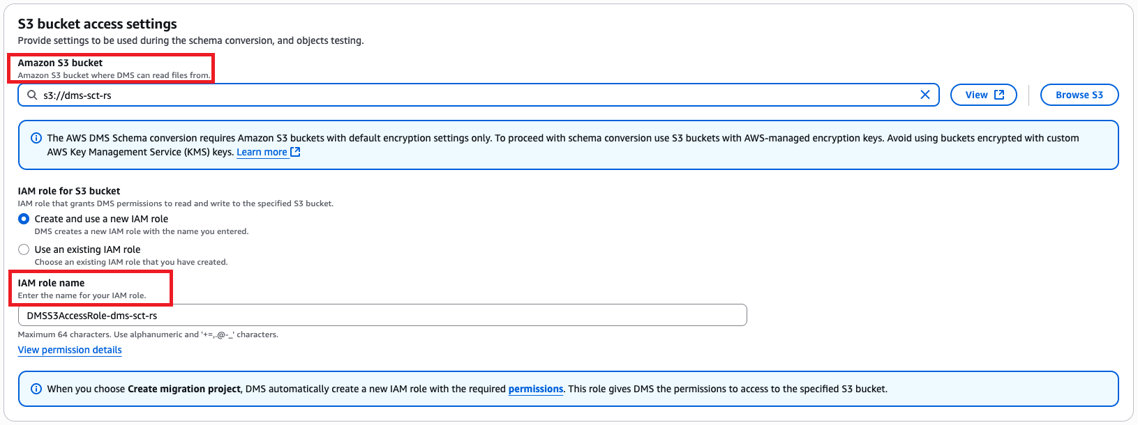
In the Schema conversion settings section, enter the S3 URL and choose the applicable IAM role.
Choose Create migration project.
Use DMS Schema Conversion to transform Oracle database objects
On the AWS DMS console, choose Migration projects in the navigation pane.
Choose the migration project you created.
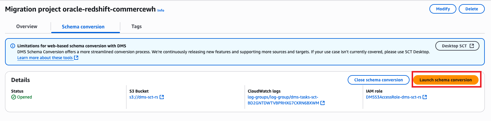
On the Schema conversion tab, choose Launch schema conversion.
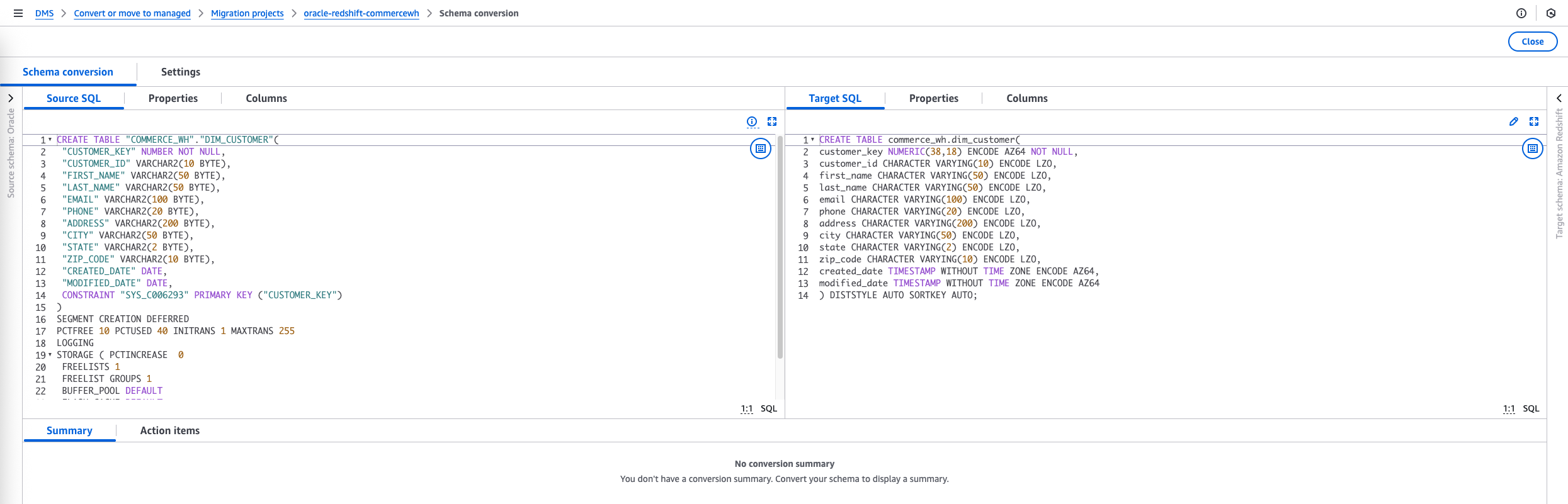
The schema conversion project will be ready when the launch is complete. The left navigation tree represents the source database, and the right navigation tree represents the target database.
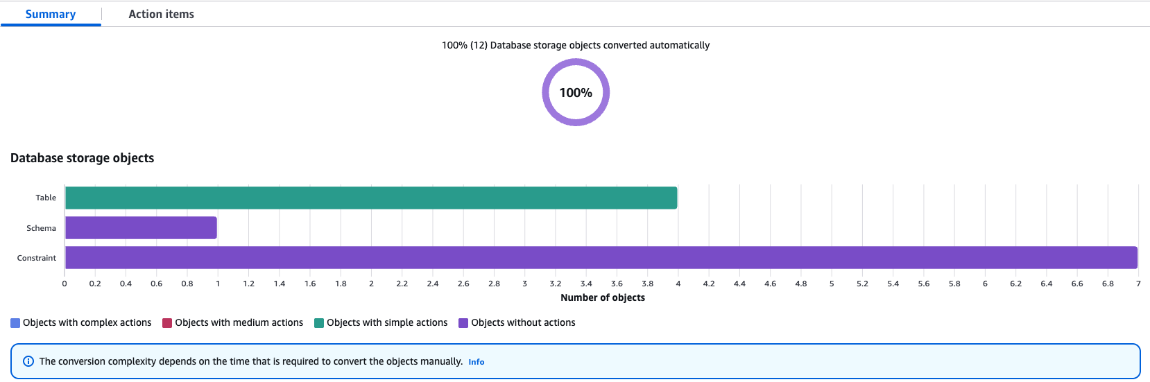
Select the objects you want to convert and then choose Convert on the Actions menu to convert the source objects to the target database.
The conversion process might take some time depending on the number and complexity of the selected objects.
You can save the converted code to the S3 bucket that you created earlier in the prerequisite steps.
To save the SQL scripts, select the object in the target database tree and choose Save as SQL on the Actions menu.
After you finalize the scripts, run them manually in the target database.
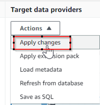
Alternatively, you can apply the scripts directly to the database using DMS Schema Conversion. Select the specific schema in the target database, and on the Actions menu, choose Apply changes.
This will apply the automatically converted code to the target database.
If some objects require action items, DMS Schema conversion flags them and provides details of action items. For the items that require resolution, perform manual changes and apply the converted changes directly to the target database.
Perform data migration
The migration from Oracle Database to Amazon Redshift using Oracle GoldenGate begins with an initial load process, where Oracle GoldenGate’s Extract process captures the existing data from the Oracle source tables and sends this data to the Replicat process, which loads it into Redshift target tables through the appropriate database connectivity. Simultaneously, Oracle GoldenGate’s CDC mechanism tracks the ongoing changes (inserts, updates, and deletes) in the source Oracle database by reading the redo logs. These captured changes are then synchronized to Amazon Redshift in near real time through the Extract-Pump-Replicat process, facilitating data consistency between the source and target systems throughout the migration process.
Prepare source Oracle database for GoldenGate
Prepare your database for Oracle GoldenGate, including configuring connections and logging, enabling Oracle GoldenGate in your database, setting up the flashback query, and managing server resources.
To handle this situation, configure Extract to generate trail records with the column values (enable trandata for the columns). Alternatively, you can disable this check by setting gg.abend.on.missing.columns=false, which may result in unintended NULLs on the target database.When gg.abend.on.missing.columns=true, Replicat process on Oracle GoldenGate for BigData fails and returns the following error for compressed update records:
ERROR OGG-15051 Java or JNI exception: java.lang.IllegalStateException: The UPDATE operation record in the trail at pos[0/XXXXXXX] for table [SCHEMA.TABLENAME] has missing columns.
Install Oracle GoldenGate software on Amazon EC2
You must run Oracle GoldenGate on EC2 instances. The instances must have adequate CPU, memory, and storage to handle the anticipated replication volume. For more details, refer to Operating System Requirements. After you determine the CPU and memory requirements, select a current generation EC2 instance type for Oracle GoldenGate.
When the EC2 instance is up and running, download the following Oracle GoldenGate software from the Oracle GoldenGate Downloads page:
The initial load configuration transfers existing data from Oracle Database to Amazon Redshift. Complete the following configuration steps:
Create an initial load extract parameter file for the source Oracle database using GoldenGate for Oracle. The following code is the sample file content:
Add the EXTRACT on the GoldenGate for Oracle prompt by running the following command:
ADD EXTRACT INITLE11, SOURCEISTABLE

GGSCI (ip-**-**-**-**.us-west-2.compute.internal) 1> info INITLE11

Extract    INITLE11  Initialized  2025-07-08 03:44   Status STOPPED
Checkpoint Lag       Not Available
Log Read Checkpoint  Not Available
                     First Record         Record 0
Task                 SOURCEISTABLE
Create a Replicat parameter file for the target Redshift database for the initial load using GoldenGate for Big Data. The following code is the sample file content:
# Add Extract and Register (EXTPRD)

ADD EXTRACT EXTPRD, INTEGRATED TRANLOG, BEGIN NOW

REGISTER EXTRACT EXTPRD DATABASE

ADD EXTTRAIL /u01/app/oracle/product/21.3.0/oggcore_1/dirdat/ep, EXTRACT
EXTPRD

GGSCI (ip-**-**-**-**.us-west-2.compute.internal) 3>  info EXTPRD

Extract    EXTPRD    Initialized  2025-07-08 03:50   Status STOPPED
Checkpoint Lag       00:00:00 (updated 00:00:36 ago)
Log Read Checkpoint  Oracle Integrated Redo Logs
                     2025-07-08 03:50:33
Create an Extract Pump parameter file for the source Oracle database to send the trail files to the target Redshift database. The following code is the sample file content:
# Pump process addition

ADD EXTRACT PMPPRD, EXTTRAILSOURCE /u01/app/oracle/product/21.3.0/oggcore_1/dirdat/ep

ADD RMTTRAIL /home/ec2-user/ogg_bd/dirdat/pt, EXTRACT PMPPRD

GGSCI (ip-**-**-**-**.us-west-2.compute.internal) 4> info PMPPRD

Extract    PMPPRD    Initialized  2025-07-08 03:51   Status STOPPED
Checkpoint Lag       00:00:00 (updated 00:00:09 ago)
Log Read Checkpoint  File /u01/app/oracle/product/21.3.0/oggcore_1/dirdat/ep000000000
                     First Record  RBA 0
Configure Oracle GoldenGate Redshift handler to apply changes to target
To configure an Oracle GoldenGate Replicat to send data to a Redshift cluster, you must set up a Redshift properties file and a Replicat parameter file that defines how data is migrated to Amazon Redshift. Complete the following steps:
Configure the Replicat properties file (rs.props), which consists of an S3 event handler and Redshift event handler. The following is an example Replicat properties file configured to connect to Amazon Redshift:
To authenticate Oracle GoldenGate’s access to the Redshift cluster for data load operations, you have two options. The recommended and more secure method is to use IAM role authentication by configuring the gg.eventhandler.redshift.AwsIamRole property in the properties file. This approach provides more secure, role-based access. Alternatively, you can use access key authentication by setting the environment variables AWS_ACCESS_KEY_ID and AWS_SECRET_ACCESS_KEY. For more information, refer to the Oracle GoldenGate for BigData documentation.
Create a Replicat parameter file for the target Redshift database using Oracle GoldenGate for BigData. The following code is the sample file content:
# Add Replicat
ADD REPLICAT RSPRD, EXTTRAIL /home/ec2-user/ogg_bd/dirdat/pt, BEGIN NOW

GGSCI (ip-**-**-**-**.us-west-2.compute.internal) 3> info RSPRD

Replicat   RSPRD     Initialized  2025-07-08 03:52   Status STOPPED
Checkpoint Lag       00:00:00 (updated 00:00:07 ago)
Log Read Checkpoint  File /home/ec2-user/ogg_bd/dirdat/pt000000000
                     2025-07-08 03:52:48.471461
Start initial load and change sync
First start the change sync extract and data pump on the source Oracle database. This will start capturing changes while you perform the initial load.
In the GoldenGate for Oracle GGSCI utility, start EXTPRD and PMPPRD:
GGSCI (ip-**-**-**-**.us-west-2.compute.internal as ggsuser@ORCL) 13> start EXTPRD

Sending START request to Manager ...
Extract group EXTPRD starting.


GGSCI (ip-**-**-**-**.us-west-2.compute.internal as ggsuser@ORCL) 15> start PMPPRD

Sending START request to Manager ...
Extract group PMPPRD starting.
Do not start Replicat at this point.
Record the Source System Change Number (SCN) from the Oracle database, which serves as the starting point for replication on the target system:
select current_scn from v$database;

CURRENT_SCN
13940177
Start the initial load Extract process, which will automatically trigger the corresponding initial load Replicat on the target system:
GGSCI (ip-**-**-**-**.us-west-2.compute.internal as ggsuser@ORCL) 21> start INITLE11

Sending START request to Manager ...
Extract group INITLE11 starting.
Monitor the initial load completion status by executing the following command on the GoldenGate for BigData GGSCI utility. Make sure the initial load process has completed successfully before proceeding to the next step. The report will indicate the load status and potential errors that need attention.
VIEW REPORT INITLR11
Start the change synchronization Replicat RSPRD using the previously captured SCN to facilitate continuous data replication:
GGSCI (ip-**-**-**-**.us-west-2.compute.internal) 17> start RSPRD , aftercsn 13940177

Sending START request to Manager ...
Replicat group RSPRD starting.
Refer to the Oracle GoldenGate documentation for Amazon Redshift handlers to learn more about its detailed functionality, unsupported operations, and system limitations.
When transitioning from initial load to continuous replication in an Oracle database to Amazon Redshift migration using Oracle GoldenGate, it’s crucial to properly manage data collisions to maintain data integrity. The key is to capture and use an appropriate SCN that marks the exact point where initial load ends and CDC begins. Without proper collision handling, you might encounter duplicate records or missing data during the transition period. Implementing appropriate collision handling mechanisms makes sure duplicate records are properly managed without causing data inconsistencies in the target system. For more information on HANDLECOLLISIONS, refer to the Oracle GoldenGate documentation.
Clean up
When the migration is complete, complete the following steps:
Stop and remove Oracle GoldenGate processes (EXTRACT, PUMP, REPLICAT).
Delete EC2 instances used for Oracle GoldenGate.
Remove IAM roles created for migration.
Delete S3 buckets used for DMS Schema Conversion (if no longer needed).
Update application connection strings to point to the new Redshift cluster.
Conclusion
In this post, we showed how to modernize your data warehouse by migrating to Amazon Redshift using Oracle GoldenGate. This approach facilitates minimal downtime and provides a flexible, reliable method for transitioning your critical data workloads to the cloud. With the complexity involved in database migrations, we highly recommend testing the migration steps in non-production environments prior to making changes in production. By following the best practices outlined in this post, you can achieve a smooth migration process and set the foundation for a scalable, cost-effective data warehousing solution on AWS. Remember to continuously monitor your new Amazon Redshift environment, optimize query performance, and take advantage of the AWS suite of analytics tools to derive maximum value from your modernized data warehouse.
Modern streaming workloads are highly dynamic—traffic volumes fluctuate based on time of day, business cycles, or event-driven bursts. Customers need to dynamically scale Apache Kafka clusters up and down to maintain consistent throughput and performance without incurring unnecessary cost. For example, ecommerce platforms see sharp traffic increases during seasonal sales, and financial systems experience load spikes during market hours. Scaling clusters helps teams align cluster capacity with increased ingress throughput in response to these variations, leading to more efficient utilization and a better cost-to-performance ratio.
Amazon Managed Streaming for Apache Kafka (Amazon MSK) Express brokers are a key component to dynamically scaling clusters to meet demand. Express based clusters deliver 3 times higher throughput, 20 times faster scaling capabilities, and 90% faster broker recovery compared to Amazon MSK Provisioned clusters. In addition, Express brokers support intelligent rebalancing for 180 times faster operation performance, so partitions are automatically and consistently well distributed across brokers. This feature is enabled by default for all new Express based clusters and comes at no additional cost to customers. This capability alleviates the need for manual partition management when modifying cluster capacity. Intelligent rebalancing automatically tracks cluster health and triggers partition redistribution when resource imbalances are detected, maintaining performance across brokers.
This post demonstrates how to use the intelligent rebalancing feature and build a custom solution that scales Express based clusters horizontally (adding and removing brokers) dynamically based on Amazon CloudWatch metrics and predefined schedules. The solution provides capacity management while maintaining cluster performance and minimizing overhead.
Overview of Kafka scaling
Scaling Kafka clusters involves adding or removing brokers to the cluster while providing balanced data distribution and uninterrupted service. When new brokers are added, partition reassignment is required to evenly distribute load across the cluster. This process is typically performed manually—either through the Kafka command line tools (kafka-reassign-partitions.sh) or by using automation frameworks such as Cruise Control, which intelligently calculates and executes reassignment plans. During scale-in operations, partitions hosted on the brokers marked for removal must first be migrated to other brokers, leaving the target brokers empty before decommissioning.
Challenges of scaling Kafka dynamically
The complexity of scaling depends heavily on the underlying storage model. In deployments where broker data resides entirely on local storage, scaling involves physical data movement between brokers, which can take considerable time depending on partition size and replication factor. In contrast, environments that use tiered storage shift most of the data to remote object storage such as Amazon Simple Storage Service (Amazon S3), making scaling a largely metadata-driven operation. This significantly reduces data transfer overhead and accelerates both broker addition and removal, enabling more elastic and operationally efficient Kafka clusters.
However, scaling Kafka remains a non-trivial operation due to the interplay between storage, data movement, and broker resource utilization. When partitions are reassigned across brokers, large volumes of data must be copied over the network, often leading to network bandwidth saturation, storage bandwidth exhaustion, and elevated CPU utilization. Depending on data volume and replication factor, partition rebalancing can take several hours, during which time cluster performance and throughput might temporarily degrade and often require additional configuration to throttle the data movement. Although tools like Cruise Control automate this process, they introduce another layer of complexity: selecting the right combination of rebalancing goals (such as disk capacity, network load, or replica distribution) requires a deep understanding of Kafka internals and trade-offs between speed, balance, and stability. As a result, efficient scaling is an optimization problem, demanding careful orchestration of storage, compute, and network resources.
How Express brokers simplify scaling
Express brokers manage Kafka scaling through their decoupled compute and storage architecture. This innovative design enables unlimited storage without pre-provisioning, significantly simplifying cluster sizing and management. The separation of compute and storage resources allows Express brokers to scale faster than standard MSK brokers, enabling rapid cluster expansion within minutes. With Express brokers, administrators can adjust capacity both vertically and horizontally as needed, alleviating the need for over-provisioning. The architecture provides sustained broker throughput during scaling operations, with Express brokers capable of handling 500 MBps ingress and 1000 MBps egress on m7g.16xl instances. For more information about how the scaling process works in Express based clusters, see Express brokers for Amazon MSK: Turbo-charged Kafka scaling with up to 20 times faster performance.
Added to this faster scaling capability, when you add or remove brokers from your Express based clusters, intelligent rebalancing automatically redistributes partitions to balance resource utilization across the brokers. This makes sure the cluster continues to operate at peak performance, making scaling in and out possible with a single update operation. Intelligent rebalancing is enabled by default on new Express broker clusters and continuously monitors cluster health for resource imbalances or hotspots. For example, if certain brokers become overloaded due to uneven distribution of partitions or skewed traffic patterns, intelligent rebalancing will automatically move partitions to less utilized brokers to restore balance.
Finally, Express based clusters automate client configuration of broker bootstrap connection strings to allow clients to connect to clusters seamlessly as brokers are added and removed. Express based clusters provide three connection strings, one per Availability Zone, which are independent of the brokers in the cluster. This means clients only need to configure these connection strings to maintain consistent connections as brokers are added or removed. These key capabilities of Express based clusters—rapid scaling, intelligent rebalancing, and dynamic broker bootstrapping—are critical to enabling dynamic scaling in Kafka clusters. In the following section, we explore how we use these capabilities to automate the scaling process of Express based clusters.
On-demand and scheduled scaling
Leveraging fast scaling capabilities of Express brokers together with intelligent rebalancing, you can build a flexible and dynamic scaling solution to optimize your Kafka cluster resources. There are two primary approaches for automatic scaling that balance performance needs with cost efficiency: on-demand and scheduled scaling.
On-demand scaling
On-demand scaling tracks cluster performance and responds to capacity demands. This approach addresses scenarios where workload patterns experience traffic spikes. On-demand scaling tracks Amazon MSK performance indicators as CPU utilization and network ingress and egress throughput per broker. Beyond these infrastructure metrics, the solution also supports using CloudWatch metrics to enable business-logic-driven scaling decisions.
The solution evaluates the performance metrics continuously against configurable thresholds to determine when scaling actions are necessary. When brokers operate above capacity thresholds consistently over a period of time, it invokes an Amazon MSK API to increase the broker count of the cluster. The solution in this post currently supports horizontal scaling (adding and removing brokers) only. Intelligent rebalancing will then automatically redistribute the partitions to spread the load across the new brokers that are added. Similarly, when utilization drops below thresholds, the solution invokes an Amazon MSK API to remove brokers. The rebalancing process automatically moves partitions from the broker marked for removal to other brokers in the cluster. This solution requires topics to have sufficient partitions to support rebalancing to new brokers as brokers are added.
The following diagram illustrates the on-demand scaling workflow.
Scheduled scaling
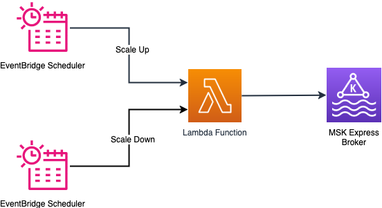
Scheduled scaling adjusts cluster capacity using time-based triggers. This approach is useful for applications with traffic patterns that correlate with business hours or schedules. For example, ecommerce platforms benefit from scheduled scaling during peak sale periods when customer activity peaks. Scheduled scaling is also useful for customers who want to avoid cluster modification operations during business hours. This solution uses a configurable schedule to scale out the cluster capacity before business hours to handle the anticipated traffic and scale in after business hours to reduce costs. This particular solution currently supports horizontal scaling (adding/removing brokers) only. With scheduled scaling, you can handle specific scenarios such as weekday business hours, weekend maintenance windows, or specific dates. You can also specify the desired number of brokers at scale-out and scale-in.
The following diagram illustrates the scheduled scaling workflow.
Solution overview
This solution provides scaling automation for Express brokers through two approaches:
On-demand scaling – Tracks built-in cluster performance metrics or custom CloudWatch metrics and adjusts broker capacity when thresholds are crossed
Scheduled scaling – Scales clusters based on specific schedules
In the following sections, we provide the implementation details for both scaling methods.
Prerequisites
Complete the following steps as prerequisites:
Create an Express cluster with intelligent rebalancing enabled. The intelligent rebalancing feature is required for this solution to work. Note the Amazon Resource Name (ARN) of the cluster.
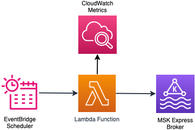
The solution uses an AWS Lambda function that is triggered by an Amazon EventBridge scheduler periodically. The Lambda function checks the cluster state and time since the last broker addition or removal was done. This is done to determine if the cluster is ready to scale. If the cluster is ready for scaling, the function collects the CloudWatch metrics that need to be evaluated to make the scaling decision. Based on the scaling configuration and using the metrics in CloudWatch, the function evaluates the scaling logic and executes the scaling decision. The scaling decision can lead to addition or removal of brokers to the cluster. In both cases, intelligent rebalancing handles partition distribution across brokers without manual intervention. You can find more details of the scaling logic in the GitHub repo.
The following diagram illustrates the architecture of the on-demand scaling solution.
Deploy on-demand scaling solution
Follow these steps to deploy the on-demand scaling infrastructure. For this post, we demonstrate the on-demand scale-out functionality.
Modify the thresholds to match your MSK broker instance size and business requirements by editing src/config/on_demand_scaling_config.json. Refer to the configuration documentation for more details of the configuration options available. By default, on_demand_scaling_config.json considers the express.m7g.large broker instance size. Therefore the scale-in/scale-out ingress/egress thresholds are configured at 70% of the recommended sustained throughput for the instance size.
Bootstrap your environment for use with the AWS CDK.
The monitoring_frequency_minutes parameter controls how often the EventBridge scheduler invokes the scaling logic Lambda function to evaluate cluster metrics.
The deployment creates the AWS resources required to run the on-demand scaling solution. The details of the resources created are shown in the output of the command.
Create a Kafka topic in the cluster. Update the following command for the specific authentication method in Amazon MSK. Refer to the Amazon MSK Labs workshop for more details.
Topics should have a sufficient number of partitions that can be distributed across a larger set of brokers.
Generate load on the MSK cluster to trigger and verify the scaling operations. You can use an existing application that drives load to your cluster. You can also use the kafka-producer-perf-test.sh utility that is bundled as part of the Kafka distribution to generate load:
Monitor the scaling operations by tailing the Lambda function logs:
aws logs tail /aws/lambda/MSKOnDemandScalingStack-MSKScalingFunction  \
--follow --format short
In the logs, look for the following messages to identify the exact times when scaling operations occurred. The log statements above these messages show the rationale behind the scaling decision:
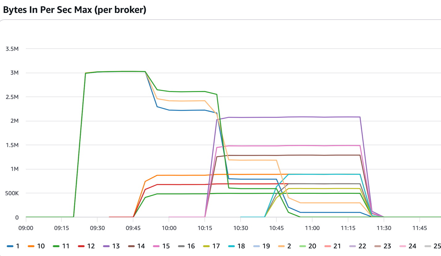
The solution also creates a CloudWatch dashboard that provides visibility into scaling operations and many other broker metrics. The link to the dashboard is shown in the output of the cdk deploy command.
The following figure shows a cluster that started with three brokers. After the 09:15 mark, it received consistent inbound traffic, which exceeded the thresholds set in the solution. The solution added three more brokers that came into service at around the 09:45 mark. Intelligent rebalancing reassigned some of the partitions to the newly added brokers and the incoming traffic was split across six brokers. The solution continued adding more brokers until the cluster had 12 brokers and the intelligent rebalancing feature continued distributing the partitions across the newly added brokers.
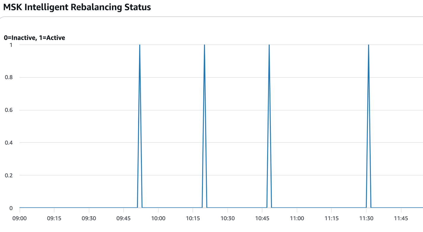
The following figure shows the times when partition rebalancing was active (value=1). In the context of this solution, that typically occurs after new brokers are added or removed and the scaling operations are complete.
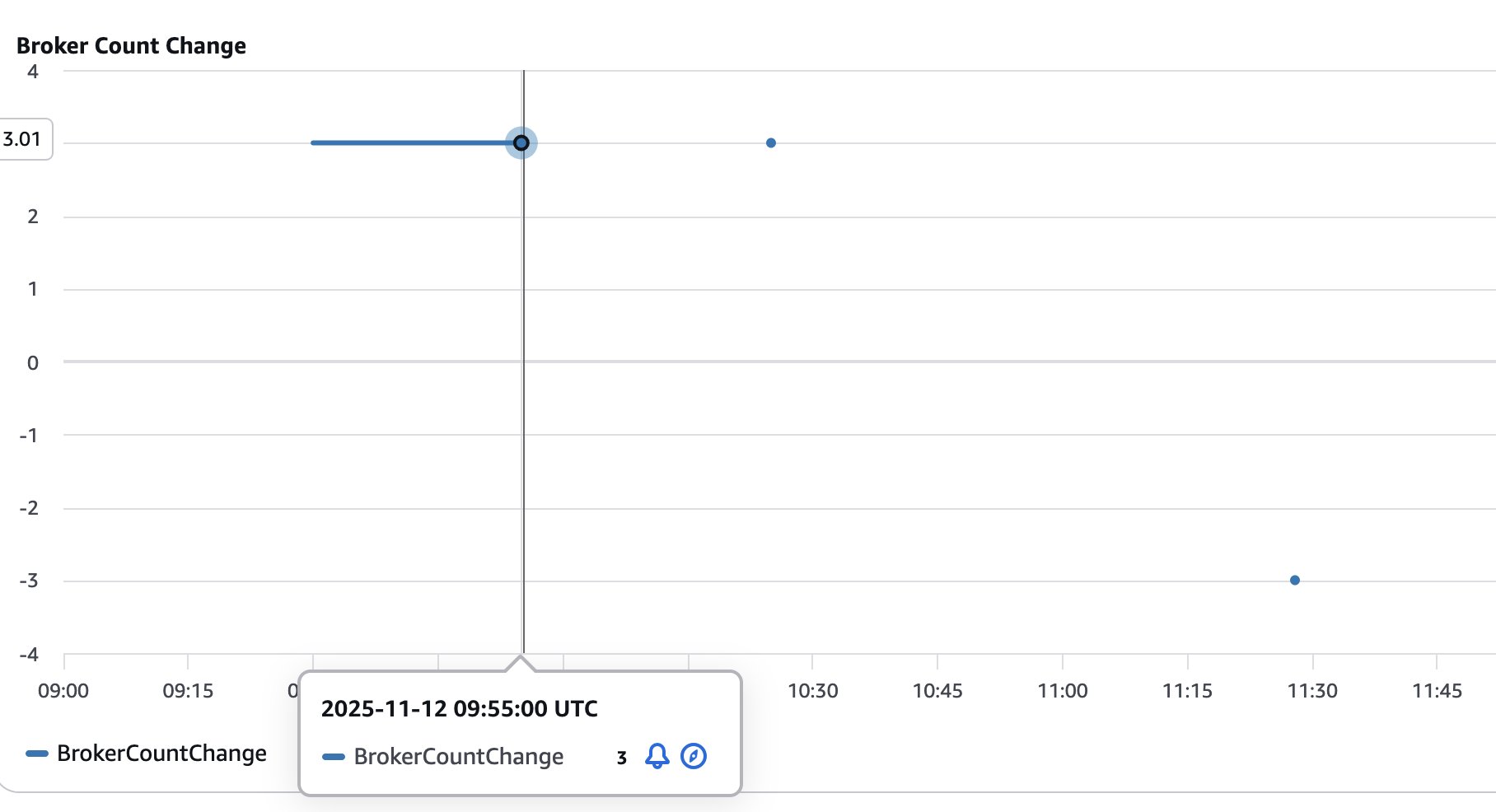
The following figure shows the number of brokers added (positive values) or removed (negative values) from the cluster. This helps visualize and track the size of the cluster as it goes through scaling operations.
Scheduled scaling solution
The scheduled scaling implementation supports timing patterns through an EventBridge schedule. You can configure timing to trigger an action using cron expressions. Based on the cron expression, the EventBridge Scheduler triggers a Lambda function at the specified time to scale out or scale in. The Lambda function performs checks if the cluster is ready for a scaling operation and performs the requested scaling operation by invoking the Amazon MSK control plane API. The service allows removing only three brokers at a time from a cluster. The solution handles this scenario by repeatedly removing the brokers in counts of three until the desired number of brokers are reached.
The following diagram illustrates the architecture of the scheduled scaling solution.
Configuration parameters
EventBridge schedules support cron expressions for precise timing control, so you can fine-tune scaling operations for specific times of day and days of the week. For example, you can configure scaling to occur at 8:00 AM on weekdays using the cron expression cron(0 8 ? * MON-FRI *). To scale in at 6:00 PM on the same days, use cron(0 18 ? * MON-FRI *). For more patterns, refer to Setting a schedule pattern for scheduled rules (legacy) in Amazon EventBridge. You can also configure the desired broker count to be reached during scale-out and scale-in operations.
Deploy scheduled scaling solution
Follow these steps to deploy the scheduled scaling solution:
Modify the scaling schedule by editing scaling/cdk/src/config/scheduled_scaling_config.json. Refer to the configuration documentation for more details of the configuration options available.
Deploy the scheduled scaling AWS CDK application:
cdk deploy MSKScheduledScalingStack \
    --app "python3 msk_scheduled_scaling_stack.py" \
    --context cluster_arn="<< ARN of the MSK Cluster >>" \
    --context stack_name="MSKScheduledScalingStack"
Test and monitor the scheduled scaling solution
The scheduled scaling is triggered as specified in the EventBridge Scheduler cron. However, if you want to test the scale-out operations, run the following command to manually invoke the Lambda function:
Monitor the scaling operations by tailing the Lambda function logs:
aws logs tail /aws/lambda/MSKScheduledScalingStack-MSKScheduledScalingFunction  \
--follow --format short
You can monitor scheduled scaling using the CloudWatch dashboard as described in the on-demand scaling section.
Review scaling configuration parameters
The configuration parameters for both on-demand and scheduled scaling are documented in Configuration Options. These configurations give you flexibility to change how and when the scaling happens. It is important to go through the configuration parameters and make sure they meet your business requirement. For on-demand scaling, you can scale the cluster based on built-in performance metrics or custom metrics (for example MessagesInPerSec).
Considerations
Keep in mind the following considerations when deploying either solution:
EventBridge notifications for scaling failures – Both on-demand and scheduled scaling solutions publish EventBridge notifications when scaling operations fail. Create EventBridge rules to route these failure events to your monitoring and alerting system to detect failures in scaling and respond to them. For details on event sources, types, and payloads, refer to the EventBridge notifications section in the GitHub repo.
Cool-down period management – Properly configure cool-down periods to prevent scaling oscillations where the cluster repeatedly scales out and scales in rapidly. Oscillations typically occur when traffic patterns have short-term spikes that don’t represent sustained demand. Oscillations can also happen when thresholds are set too close to normal operating levels. Set cool-down periods based on your workload characteristics and the scaling completion times. Also consider different cool-down periods for scale-out vs. scale-in operations by setting longer cool-down periods for scale-in operations (scale_in_cooldown_minutes) compared to scaling out (scale_out_cooldown_minutes). Test cool-down settings under realistic load patterns before production deployment to achieve optimal performance.
Cost control through monitoring frequency – The solution incurs costs for services like Lambda functions, EventBridge schedules, CloudWatch metrics, and logs that are used in the solution. Both on-demand and scheduled scaling solutions work by running periodically to check the cluster health status and if a scaling operation needs to be performed. The default 1-minute monitoring frequency provides responsive scaling but increases other costs associated with the solution. Consider increasing the monitoring interval based on your workload characteristics to balance scaling responsiveness and the cost incurred by the solution. You can change the monitoring frequency by changing the monitoring_frequency_minutes when you deploy the solution.
Solution isolation – The on-demand and scheduled scaling solutions were designed and tested in isolation to support predictable behavior and optimal performance. You can deploy either solution, but avoid running both solutions simultaneously on the same cluster. Using both approaches together can cause unpredictable scaling behavior where the solutions might conflict with each other’s scaling decisions, leading to resource contention and potential scaling oscillations. Choose the approach that best matches your workload patterns and deploy only one scaling solution per cluster.
Clean up
Follow these steps to delete the resources created by the solution. Make sure all the scaling operations that are in flight are completed before you run the cleanup.Delete the on-demand scaling solution with the following code:
In this post, we showed how to use intelligent rebalancing to scale your Express based cluster based on your business requirements without requiring manual partition rebalancing. You can extend the solution to use the specific CloudWatch metrics that your business depends on to dynamically scale your Kafka cluster. Similarly, you can adjust the scheduled scaling solution to scale out and scale in your cluster when you anticipate significant change in traffic to your cluster at specific times.To learn more about the services used in this solution, refer to the following resources:
Organizations face challenges in accessing and analyzing governed data across multiple sources through their preferred business intelligence (BI) and analytics tools while maintaining security and governance. They need a seamless way to connect their familiar tools (like Tableau, Power BI, Excel) to Amazon SageMaker‘s data assets without compromising data governance and security protocols.
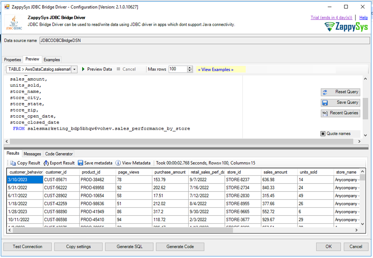
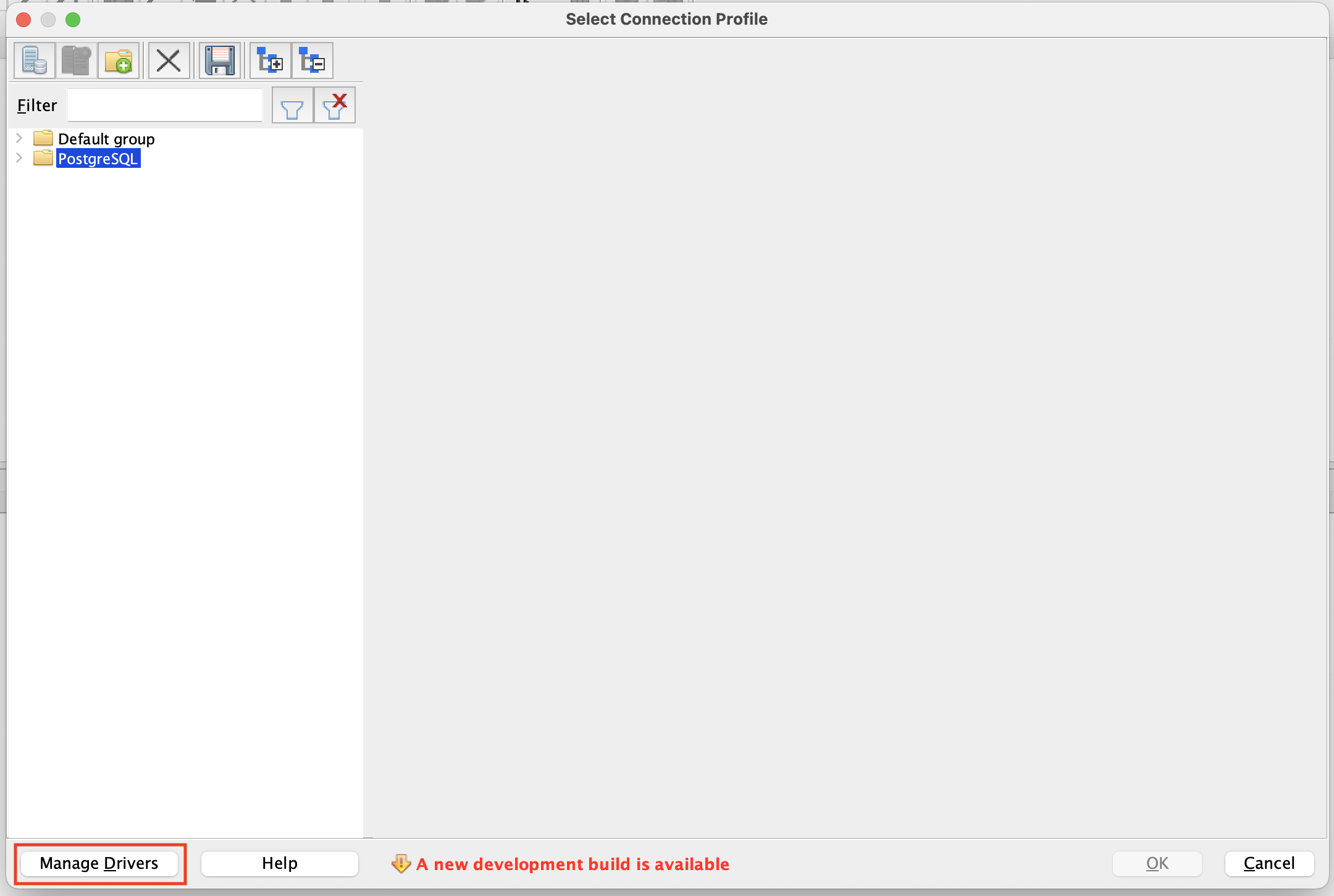
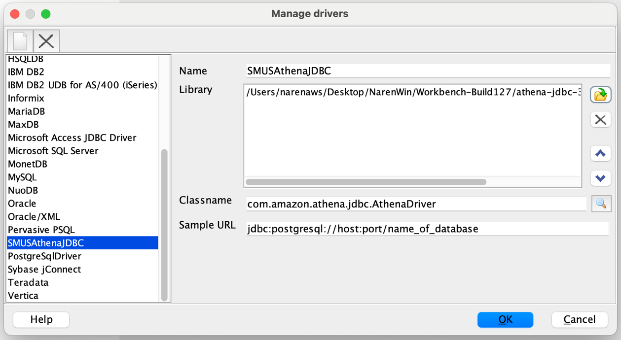
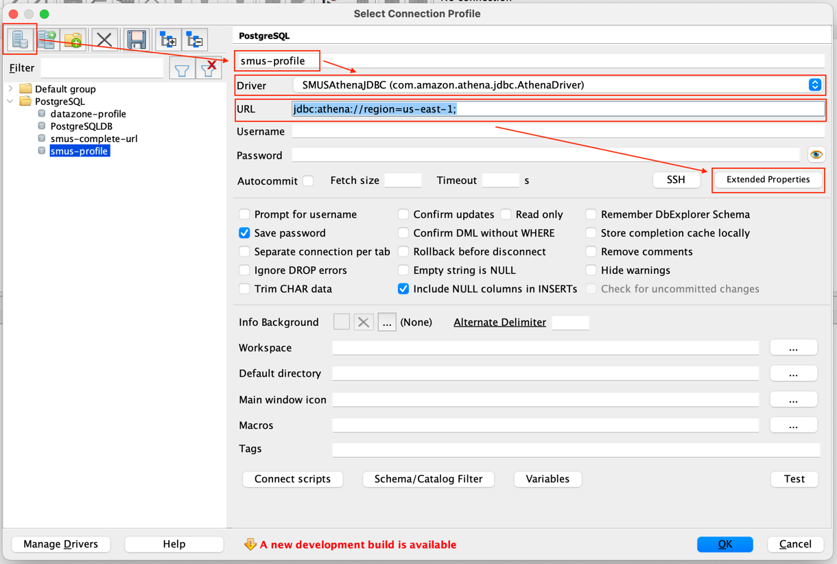
Amazon SageMaker supports authentication through the Amazon Athena JDBC driver, allowing data users to query their subscribed data lake assets via popular BI and analytics tools like Tableau, Power BI, Excel, SQL Workbench, DBeaver, and more. This integration empowers data users to access and analyze governed data within Amazon SageMaker using familiar tools, boosting both productivity and flexibility.
Customers use Amazon SageMaker Unified Studio to streamline data access and governance by enabling data users to locate and subscribe to data from multiple sources within a single project. Amazon SageMaker Unified Studio natively integrates with Amazon-specific options like Amazon Athena, Amazon Redshift, and Amazon SageMaker AI, allowing users to analyze their project governed data. With this launch of JDBC connectivity, Amazon SageMaker Unified Studio expands its support for data users, including analysts and scientists, allowing them to work in their preferred tools, whether it’s SQL Workbench, Domino, or Amazon-native solutions like Amazon Athena, while ensuring secure, governed access within Amazon SageMaker Unified Studio.
Getting Started
To get started, download and install the latest Athena JDBC driver for your tool of choice. After installation, copy the JDBC connection string from the Amazon SageMaker Unified Studio portal into the JDBC connection configuration to establish a connection from your tool. This directs you to authenticate using single sign-on (SSO) with your corporate credentials. After connecting, you can query, visualize, and share data—governed by Amazon SageMaker Unified Studio–within the tools you already know and trust.
In this post, we guide you through connecting various analytics tools to Amazon SageMaker Unified Studio using the Athena JDBC driver, enabling seamless access to your subscribed data within your Amazon SageMaker Unified Studio projects.
Solution overview
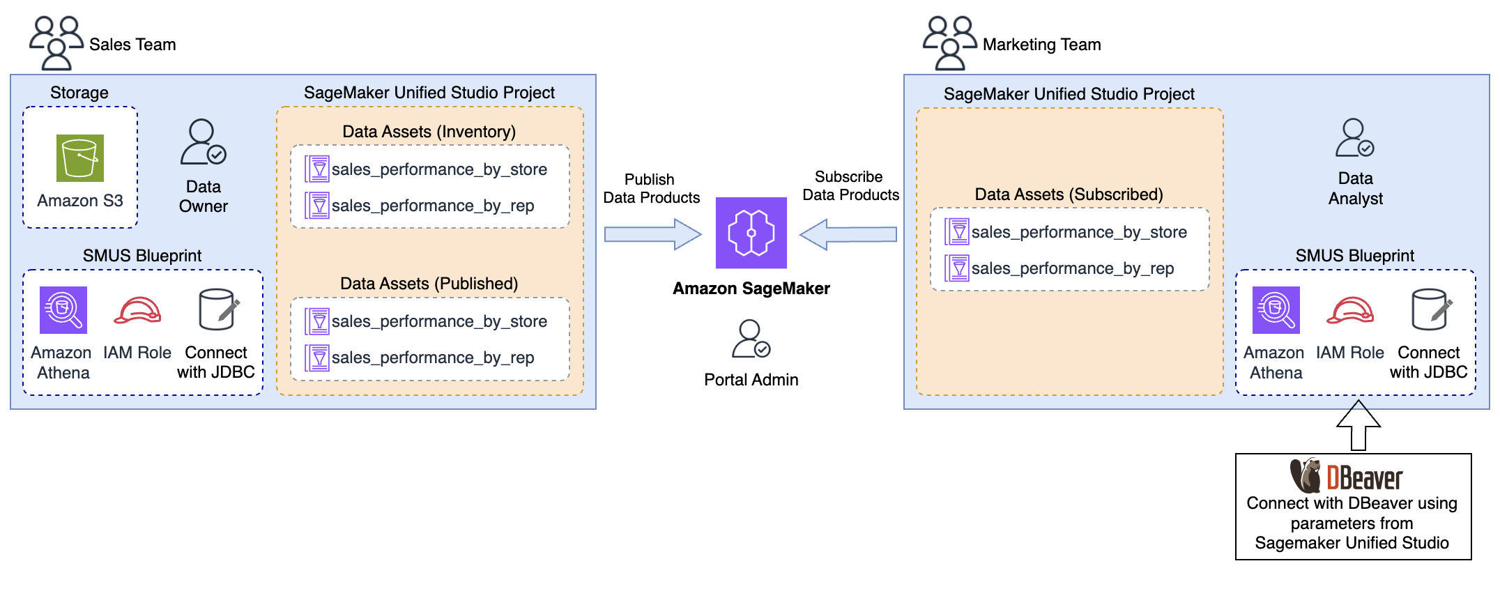
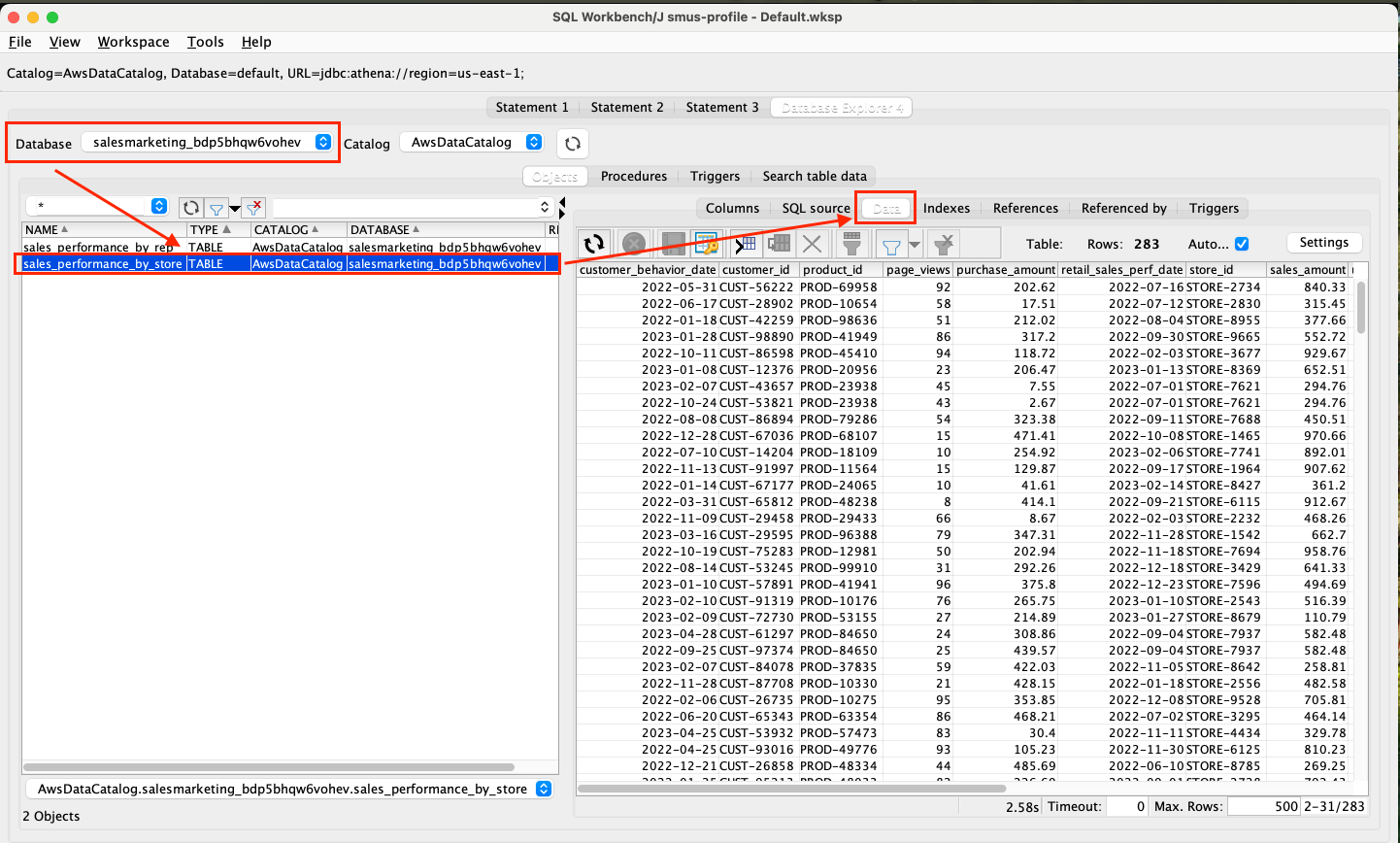
To demonstrate these capabilities, consider a use case where your marketing team wants to analyze sales data to understand patterns in sales by stores and sales representatives. To achieve this, your marketing team needs access to sales_performance_by_store, and sales_performance_by_rep data owned by the sales team. The sales team, acting as the data producer, publishes the necessary data assets to Amazon SageMaker Unified Studio, allowing the marketing team, as a consumer, to discover and subscribe to these assets.
After the subscription is approved, the data assets become available within the marketing team’s project environment in Amazon SageMaker Unified Studio. The marketing team can then use their preferred tool to perform data exploration. An example architecture of how this is done using DBeaver is shown in the following image:
Prerequisites
To follow along with this post, you need the following prerequisites in place:
Publish data assets – As the data producer from the sales team, you can now ingest individual data assets into Amazon SageMaker Unified Studio. For this use case, create a data source and import the technical metadata of two data assets – sales_performance_by_store, and sales_performance_by_rep – from AWS Glue Data Catalog. Ensure the data assets are enriched with business descriptions and published to the catalog. Note: Here we are using tables which are in the Glue catalog but with Sagemaker Lakehouse you have the option to bring assets from other sources.
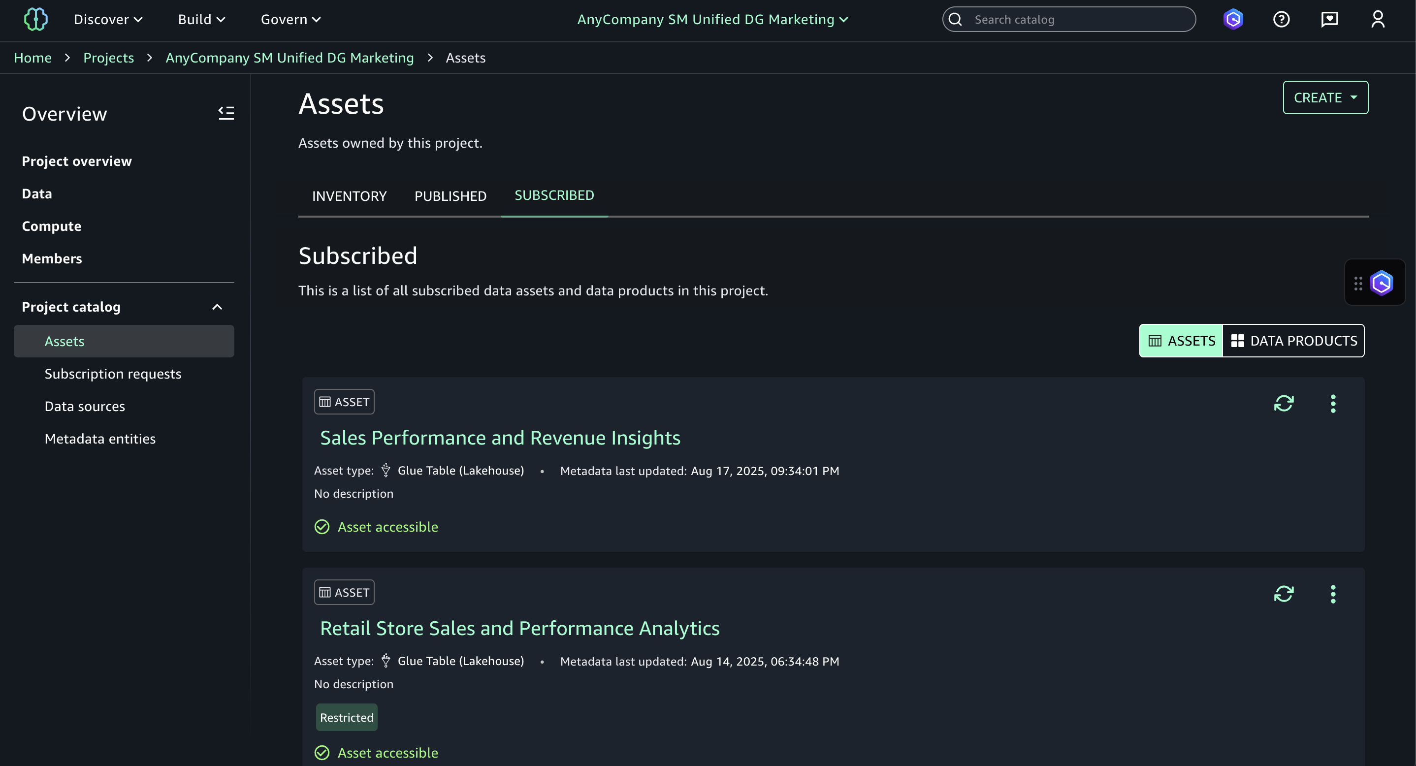
Subscribe data assets – As a data analyst from the marketing team, you can now discover and subscribe to the data assets. The data producer from the retail team reviews and approves your subscription. Upon successful fulfillment, the data assets are added to your SageMaker Unified project.
The following figure shows the subscribed assets added to the subscribed assets section in your marketing project catalog.
In the following sections, we walk you through the steps to configure DBeaver to consume the subscribed assets from Amazon SageMaker Unified Studio.
Configuring DBeaver to access subscribed data assets
In this section, you configure DBeaver to access the subscribed assets from the Marketing project
To configure DBeaver:
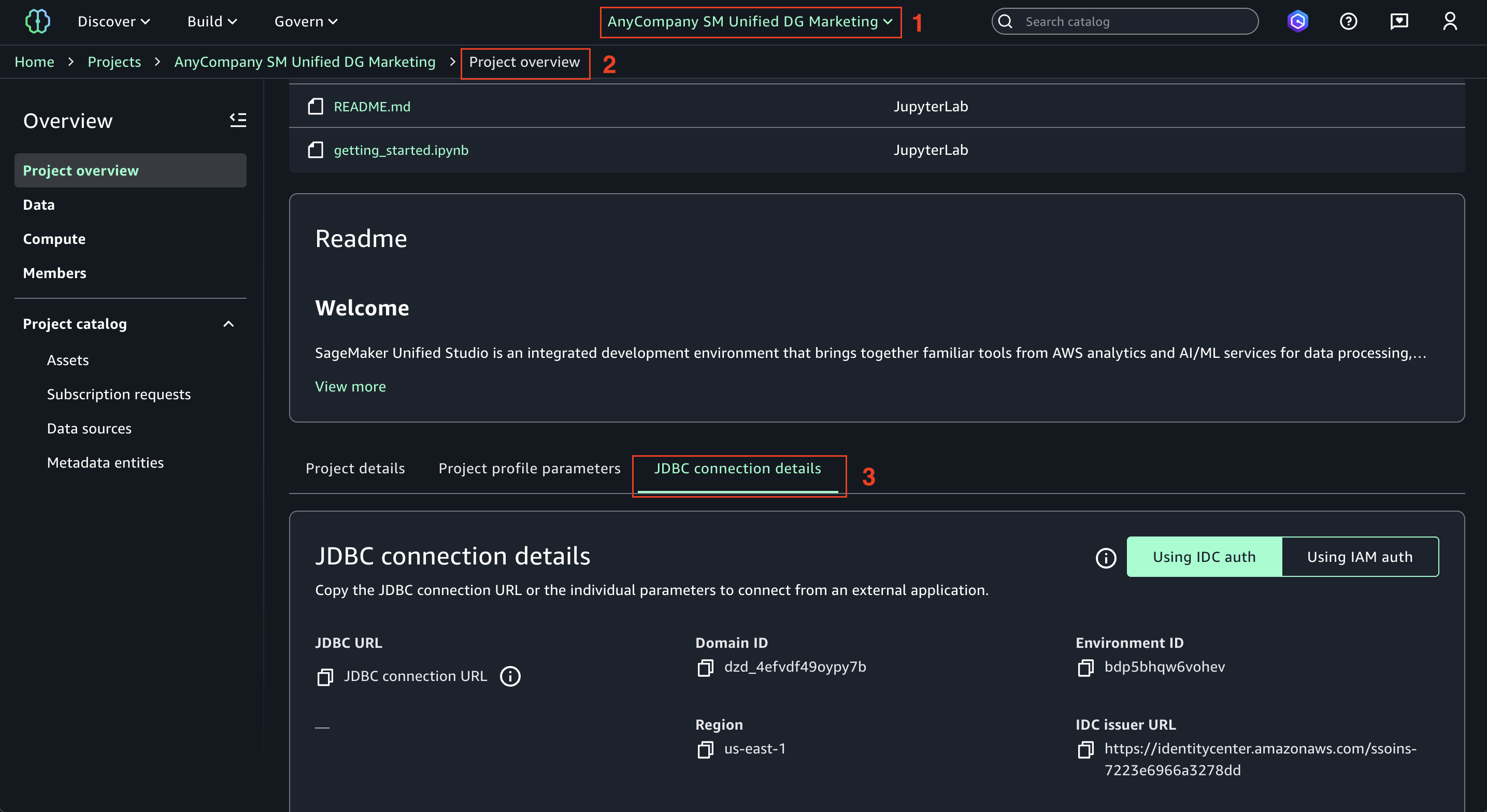
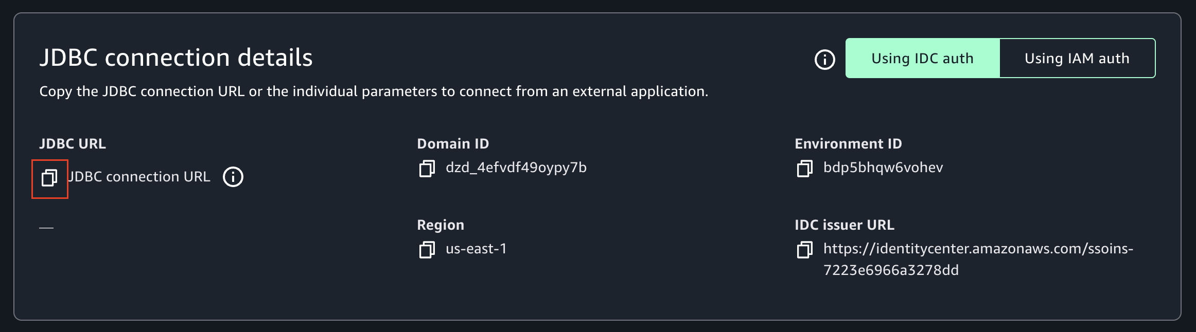
Connect with JDBC: In the Amazon SageMaker Unified Studio, (1) open the Marketing project, (2) on the Project overview screen, (3) choose JDBC connection details tab.
Copy the JDBC connection URL into a text editor. The URL should have the following parameters needed for configuring the database connection in DBeaver – Domain ID, Environment ID, Region, and IDC Issuer URL.
Download and install the latest Athena driver:
If DBeaver has the Athena driver pre-installed, it might be the older (v2) version. To ensure compatibility with Amazon SageMaker Unified Studio, you need the latest driver (v3), which includes the necessary authentication features.
Go to Database and then to Driver Manager in DBeaver.
Select the Athena driver and choose Edit.
Visit the Libraries tab.
Choose Download/Update to fetch the latest driver version.
If prompted, select the appropriate version and confirm the download.
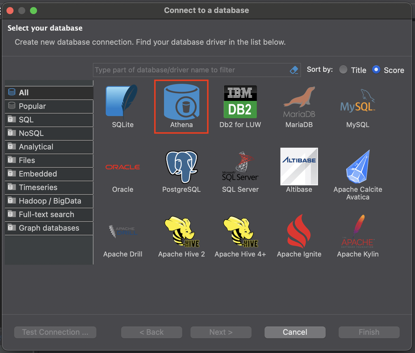
In the DBeaver SQL client, create a new database connection and select the Athena driver.
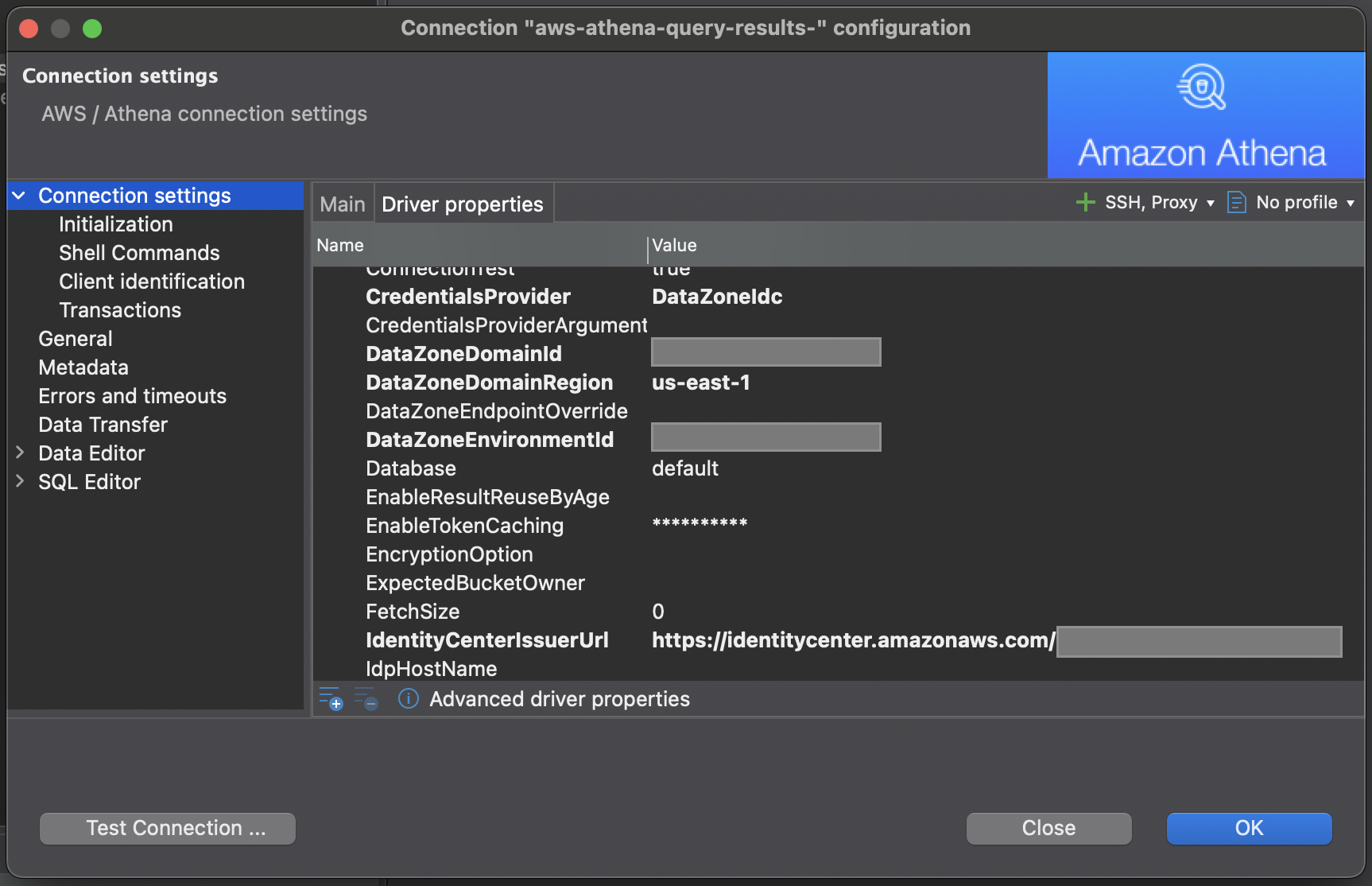
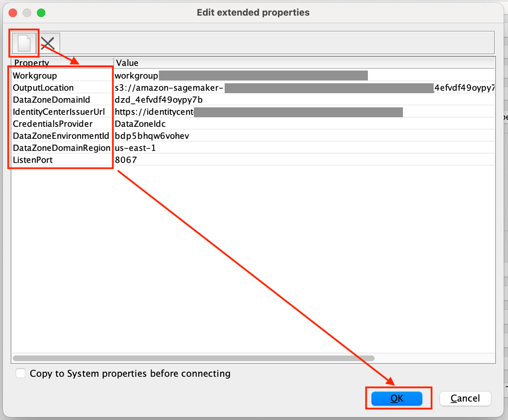
Switch to the Driver Properties tab, enter the values of the following properties that are available in the JDBC connection URL you copied from Amazon SageMaker Unified Studio. If any of these properties are not already available, you can add them and provide their respective values.
CredentialsProvider: The credentials provider to authenticate requests to AWS
DataZoneDomainId: The ID of your Amazon DataZone domain
DataZoneDomainRegion: The AWS Region where your domain is hosted
DataZoneEnvironmentId: The ID of your DefaultDataLake environment
OutputLocation: Amazon S3 path for storing query results
Region: The Region where the environment is created
Workgroup: Amazon Athena workgroup of the environment
ListenPort: Pick any four digits port number. This is the port number that listens for the IAM Identity Center response
Choose Test Connection….
You are redirected to the IAM Identity Center sign-in portal. Sign in with Marketing user credentials. If you’re already signed in through single sign-on (SSO), this step can be skipped.
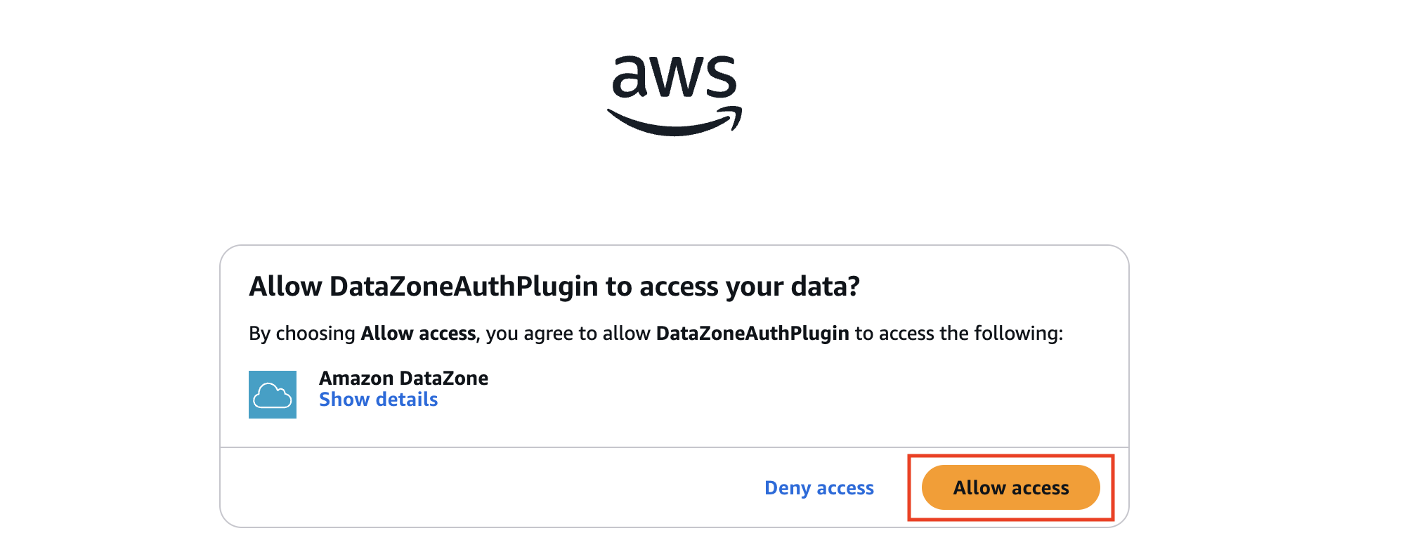
After you sign in, if you are prompted to authorize the DataZoneAuthPlugin. Choose Allow access to authorize access to Amazon DataZone from DBeaver.
After sign in completes, you see the following message. You can close the window and go to the DBeaver.
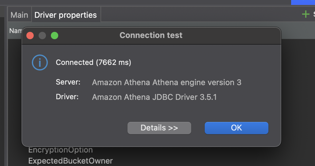
After the connection is established, the following success message appears.
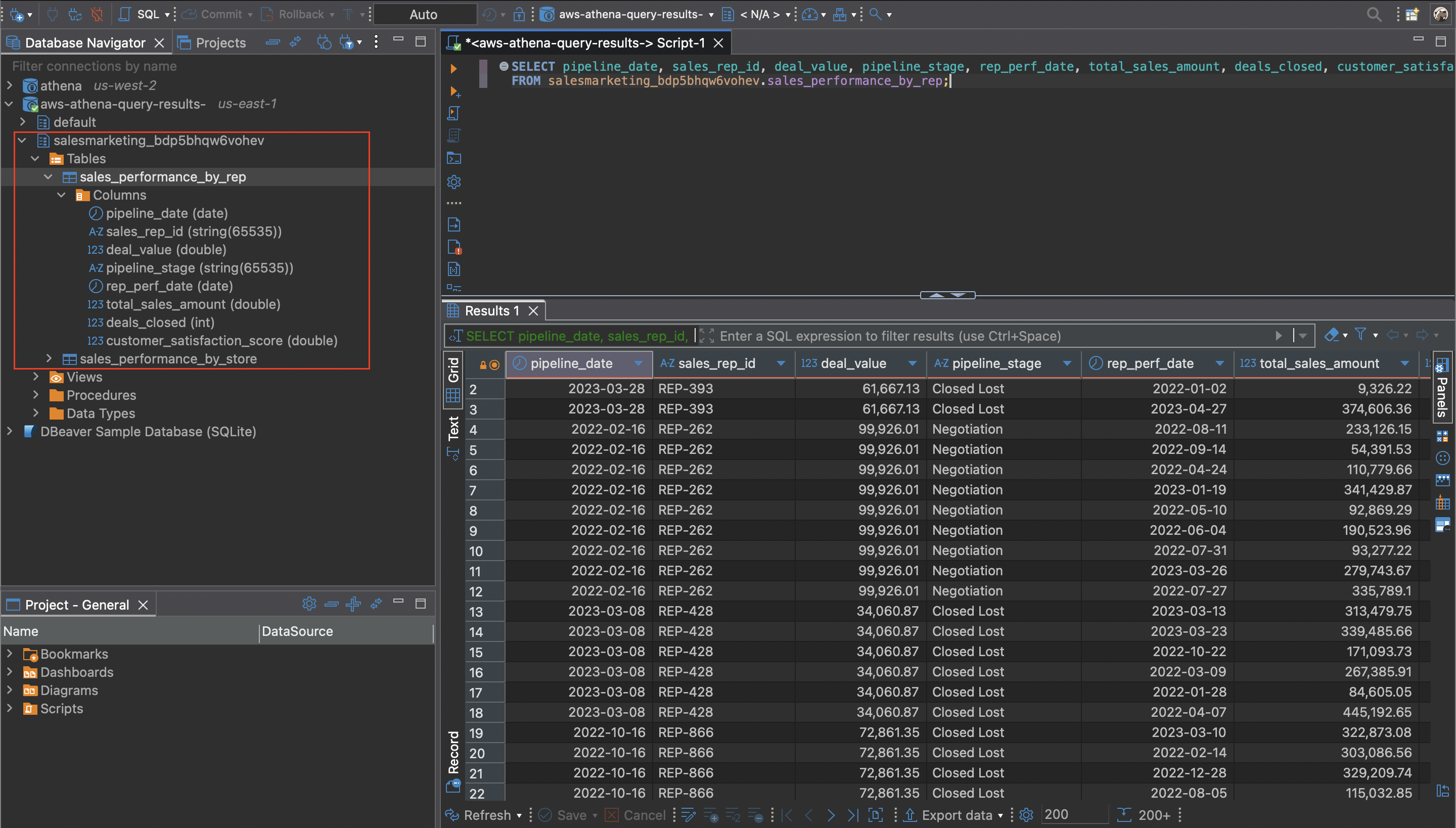
You can now view and query all subscribed assets directly within DBeaver.
These steps might also apply to other analytics tools and clients that support JDBC connections. If you’re using a different tool, you might need to adapt these instructions accordingly to ensure proper configuration and access to Amazon SageMaker Unified Studio data assets.
Integration with other applications
You can use similar steps for other BI and analytics tools that support standard database connections.
Connect to Tableau Desktop
Use the Athena JDBC driver to connect Tableau to Amazon SageMaker Unified Studio and visualize your subscribed data.To connect to Tableau Desktop:
Copy the JDBC driver file and place it in the appropriate folders for your operating system
For Mac OS: ~/Library/Tableau/Drivers
For Windows: C:\Program Files\Tableau\Drivers
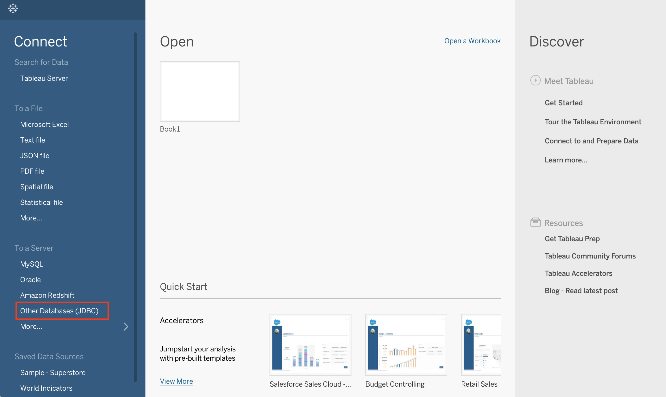
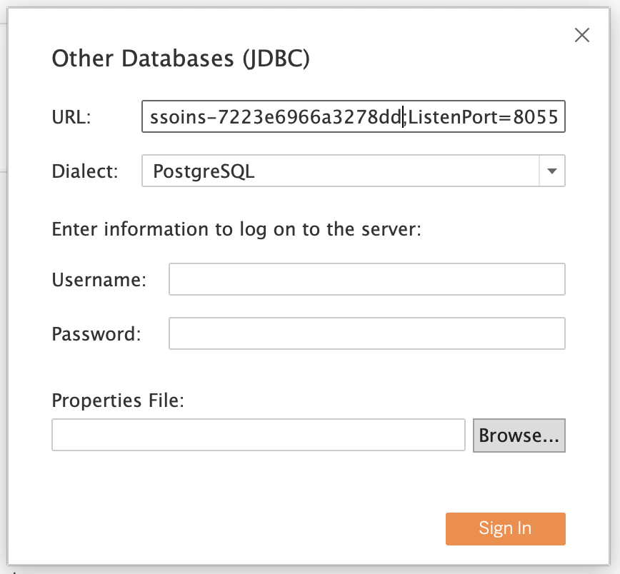
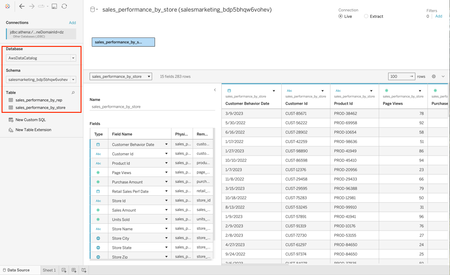
Open Tableau Desktop. From the To a Server connection menu, select Other Databases (JDBC) to connect to Amazon SageMaker Unified Studio.
Paste the JDBC connection URL you copied from the SageMaker Unified Studio portal into the URL. Leave other fields such as Dialect, Username, and Password blank and choose Sign in. If you get a port is occupied error – add “;ListenPort=8055” to the URL to change the port. You can use any port number.
This redirects you to authenticate with IAM Identity Center. Enter the credentials of the Identity Center user that you used to sign in to the SageMaker Unified Studio portal. Authorize the DataZoneAuthPlugin to access Amazon DataZone from Tableau. Once the connection is established with the success message, you can view your project’s subscribed data directly within Tableau and build dashboards.
Connect to Microsoft Power BI
Now, we look at connecting Amazon SageMaker Unified Studio with Microsoft Power BI on Windows.While Amazon Athena provides a native ODBC driver for connecting to ODBC-compatible tools like Microsoft Power BI, it currently doesn’t support Amazon SageMaker Unified Studio authentication. Therefore, in this post, we use an ODBC-JDBC bridge to connect Amazon SageMaker Unified Studio with Microsoft Power BI using the Athena JDBC driver, which supports SageMaker Unified Studio authentication.
In this post, we’re using the ZappySys driver as the ODBC-JDBC bridge. This is a third-party solution that requires a separate licensing fee, which isn’t included in the AWS solution. You can choose to use any other solution for ODBC-JDBC bridge.To connect to Power BI:
Make sure that you have administrator privileges to run the ODBC Data Source Administrator.
From the Windows Start menu, run the ODBC Data Source Administrator (the 64-bit version) using run as Administrator.
Create a New Data Source with the ZappySys JDBC Bridge Driver. You are prompted to enter your connection details.
Paste the JDBC URL you copied from the SageMaker Unified Studio portal in the Connection String, along with the driver class and JDBC driver file. Make sure that you’re using the latest Athena JDBC 3.x driver.
Choose Test Connection. A new dialog window pops up after the connection is successful.
This redirects you to authenticate with IAM Identity Center. Enter the credentials of the Identity Center user that you used to sign in to the SageMaker Unified Studio portal. Authorize the DataZoneAuthPlugin.
Choose Preview tab on ZappySys JDBC Bridge Driver window and choose one of the subscribed tables to access data.
After configuring the data source, launch Power BI. Create a blank report or use an existing report to integrate the new visuals. Choose Get Data and select the name of the data source you created. This opens a new browser window to authenticate your credentials. Allow access to authorize the DataZone Auth plugin. After authorization is complete, you can build your reports in Microsoft Power BI with the subscribed data assets.
Connect to SQL Workbench
Discover how SQL Workbench can connect to Amazon SageMaker Unified Studio for users who prefer a SQL interface to query data lake tables and views subscribed through projects in Amazon SageMaker Unified Studio.
Select the option to add a new driver. Enter a name for it, such as SMUSAthenaJDBC, and import the driver you downloaded in the previous steps.
Create a new connection profile and enter a name it, such as smus-profile. In the Driver dropdown, select the driver you configured. For the URL, enter the string jdbc:athena://region=us-east-1; (In the example, the Virginia Region is being used). Choose Extended Properties.
Under Extended Properties, add the following parameters that you copied from the SageMaker Unified Studio portal. You can also include these parameters in the JDBC (URL) connection string. Choose OK.
Workgroup
OutputLocation
DataZoneDomainId
IdentityCenterIssuerURL
CredentialsProvider
DatazoneEnvironmentId
DataZoneDomainRegain
Alos add “ListenPort” with any port number.
This redirects you to authenticate with IAM Identity Center. Enter the credentials of the Identity Center user that you used to sign in to the SageMaker Unified Studio portal. Authorize the DataZoneAuthPlugin.
After successful connection, in SQL Workbench/J, under Database Explorer, select the database from the marketing project of SageMaker unified studio. Choose a subscribed table. Select the Data tab to see the data in the table.
Cleanup
To ensure no additional charges are incurred after testing, be sure to delete the Amazon SageMaker Unified Studio domain. See Delete domains for instructions.
Conclusion
Amazon SageMaker Unified Studio continues to expand its offerings, providing you with more flexibility to access, analyze, and visualize your subscribed data. With support for the Athena JDBC driver, you can now use a wide range of popular BI and analytics tools, making data accessed through Amazon SageMaker Unified Studio more accessible than ever before. Whether you’re using Tableau, Power BI, or other familiar tools, the integration with Amazon SageMaker Unified Studio ensures that your data remains secure and accessible to authorized users.
The feature is supported in all AWS commercial Regions where Amazon SageMaker Unified Studio is currently available. Get started with our technical documentation.
Accelerating data analysis and machine learning (ML) development requires AI tools that understand your specific data environment, not just generic code generation. General-purpose AI assistants lack context about your specific data environment, creating a gap between AI capabilities and practical implementation. Data practitioners often start by looking for relevant tables, understanding relationships, and writing exploratory code before answering their first business question. Data teams still spend time translating AI-generated suggestions into working code that correctly references their actual data assets, understands their organization’s data relationships, and integrates with their existing workflows.
AWS released Amazon SageMaker Data Agent in November 2025, addressing these challenges by providing an AI assistant that’s deeply integrated within Amazon SageMaker (IAM-based domains only) with notebooks. SageMaker Data Agent has direct access to your AWS data context, including AWS Glue Data Catalog metadata, Amazon DataZone business data catalog, and your current notebook state. This helps it generate environment-aware code that works directly with your petabyte-scale data through serverless compute resources, helping you analyze massive datasets without infrastructure management overhead. With this contextual awareness, the agent creates executable analysis plans from natural language prompts that specifically reference your actual tables, data types, and analytical needs, while maintaining reasoning throughout multi-step analyses. Importantly, the agent performs these operations securely within the AWS environment, using built-in governance controls, Amazon Identity and Access Management (IAM) policies, and data security features to make sure your data doesn’t leave your organizational boundaries. By operating within your Amazon SageMaker Unified Studio interface, it reduces context-switching between AI assistants and your development environment, improving how you interact with your analytics and ML workflows.
In this post, we demonstrate the capabilities of SageMaker Data Agent, discuss the challenges it addresses, and explore a real-world example analyzing New York City taxi trip data to see the agent in action.
Challenges in data workflows
General AI tools can generate code snippets, but you still face three key challenges when applying these to your specific data environments:
Contextual disconnect – Standard AI assistants generate generic code referencing hypothetical tables like customers rather than your actual tables like customer_activity_prod, forcing extensive modifications to work with your data environment.
Complex data environment – Many enterprises work with complex data environments containing numerous tables and large-scale data stores, making it extremely difficult to locate relevant data assets for analysis. You must navigate complex catalog structures, understand table relationships, and determine which subset of data is relevant for your specific analytical needs before you can begin actual analysis.
Language and syntax barriers – You must work across multiple programming languages and query syntaxes during analysis workflows. Some might excel in SQL but struggle with Python, while others might be Python experts but have limited PySpark knowledge.
Additionally, you face challenges around data quality validation, data governance, and performance optimization. SageMaker Data Agent addresses these fundamental workflow challenges while adapting to your requirements.
Solution overview
SageMaker Data Agent addresses these key challenges through its context-aware architecture and deep AWS integration. In this section, we discuss how it works.
Context-aware understanding
SageMaker Data Agent builds a detailed understanding of your specific data environment and references your actual tables through two parallel processes. SageMaker Data Agent is embedded within your AWS data environment, allowing it to understand what you’re asking, what data you have available, how it’s structured, and how it relates to your analytical objectives. The following are the two ways the agent achieves this contextual understanding:
Integrated data environment – SageMaker Data Agent exists within the same integrated environment as your data, harnessing the power of your AWS infrastructure. It begins by exploring the AWS Glue Data Catalog and the Amazon DataZone business data catalog, which reveal business metadata, glossaries, and relationships, enabling it to reference your actual tables rather than generic placeholders. This intelligence extends to working directly with your full datasets where they naturally reside, preserving your existing security policies and access controls without requiring data movement. The agent integrates with Amazon Simple Storage Service (Amazon S3), Amazon Athena, and Amazon SageMaker AI to use their respective capabilities for data storage, query processing, and ML while adapting to your data environment. This lets you process petabyte-scale data through serverless compute resources with the agent acting as an intelligent interface to your complete data environment.
Notebook context awareness – Simultaneously, the agent examines your current notebook state, including existing dataframes, imported libraries, previous cell results, and ML artifacts. This context awareness makes sure generated code works with your specific environment without extensive modifications.
Language and syntax flexibility
SageMaker Data Agent resolves language and syntax barriers by selecting the optimal language for each analytical task. The agent can switch between SQL for efficient data querying and Python and PySpark for complex transformations and ML operations without requiring practitioners to manually translate between languages. This avoids language barriers, because the agent automatically selects and generates the appropriate code syntax, whether SQL, Python, or PySpark, based on the specific analytical or ML task at hand.
SageMaker Data Agent provides four key capabilities that work together to give you control over complex analyses:
When handling complex requests, the agent creates structured analysis plans by breaking them into logical steps with clear reasoning for each operation.
At each stage, you have intermediate validation points where you can review and approve each step before proceeding to the next.
Throughout multi-step analyses, the agent maintains consistent context, retaining understanding of your data environment and previous steps.
Most importantly, you maintain human-in-the-loop control with full oversight and the ability to modify any generated code to match your specific requirements.
Interaction modes
SageMaker Data Agent provides two interaction modes optimized for different analytical tasks: the Agent Panel and in-line assistance.
The Agent Panel supports comprehensive analytical tasks by breaking them down into structured steps, each with generated code that builds on previous results. When you submit a request such as “perform customer segmentation,” the agent identifies relevant tables, understands their relationships, and creates a complete analysis workflow with intermediate review points. The following screenshot illustrates this example.
In-line assistance mode supports direct cell modifications, one-click error fixes, and keyboard shortcuts (Alt+A for Windows/Linux, Opt+A for Mac) that maintain your coding flow. You can quickly enhance existing code or fix errors without leaving your current notebook context, improving productivity during iterative development. You can code directly within notebook cells by using the inline prompt interface, as illustrated in the following screenshot. Use in-line assistance for focused tasks like specific queries or visualizations directly within cells.
Execution and control
Throughout the process, you maintain execution control. You can review generated plans before execution, execute steps individually with intermediate result review, modify code as needed for your specific requirements by providing feedback, and get AI-powered error diagnosis and fixes using the Fix with AI option when issues arise. This human-in-the-loop approach makes sure you maintain oversight while benefiting from AI assistance.
The following screenshots demonstrate how the Fix with AI feature works in practice, showing how the agent diagnoses code errors and provides corrected solutions with explanations.
By bringing together context-aware understanding, reasoning, and interaction modes within your existing AWS environment, SageMaker Data Agent improves how you work. It removes the traditional friction between AI assistance and your actual data environment, providing direct access to petabyte-scale data with no operational overhead. This combination helps you shift your focus from repetitive setup tasks to high-value analysis and decision-making, accelerating insights while maintaining control over the analytical process.
Getting started with SageMaker Data Agent
Now that you understand how SageMaker Data Agent works, let’s see these capabilities in action. Getting started with SageMaker Data Agent is straightforward. For detailed setup instructions, refer to New one-click onboarding and notebooks with a built-in AI agent in Amazon SageMaker Unified Studio. It provides step-by-step guidance on setting up your environment and beginning your journey with SageMaker Data Agent.
To get the most from SageMaker Data Agent, begin by asking clear, specific questions about your data rather than generic requests. Provide context about your analytical goals so the agent can tailor its responses to your specific use case. Always review and validate generated code before execution, using the agent’s built-in explanations to understand the approach. For complex analyses, take advantage of the agent’s reasoning capabilities that can break down multi-step processes and explain the logic behind each recommendation.
NYC taxi trip analysis
In this section, we demonstrate how SageMaker Data Agent helps analyze the NYC Taxi Trip dataset, a collection of over 1.2 billion taxi trips (approximately 63.7 GB) throughout New York City with information on pickup/drop-off locations, timestamps, trip distances, fare amounts, payment types, and passenger counts.
If you’re looking to try a simpler end-to-end flow before diving into this large-scale analysis, SageMaker Unified Studio provides a sample database with pre-loaded customer churn data. You can perform similar analytical workflows on this smaller dataset to quickly familiarize yourself with the agent’s capabilities before working with larger, more complex datasets. To explore this dataset, complete the following steps:
On the SageMaker Unified Studio console, choose Data in the navigation pane.
In the data explorer, under Catalogs, select AwsDataCatalog.
Select sagemaker_sample_db.
Select the churn table from the tables list.
NYC Taxi Trip dataset
The NYC Taxi Trip dataset is publicly available in Amazon S3 at s3://aws-data-analytics-workshops/shared_datasets/nyc_taxi_trips_parquet/.
To replicate this, you can work with this dataset in two ways:
Catalog it beforehand (recommended for repeated analysis)
Provide the S3 path directly in your prompt (quickest for one-time exploration)
For this demonstration, we used SageMaker Data Agent to catalog the dataset prior to analysis.
Our analysis approach
For this demonstration, we asked SageMaker Data Agent to perform a comprehensive analysis on the cataloged taxi trip data to uncover business insights. We used the following prompt:
Using Apache Spark, analyze the NYC taxi trips dataset to extract meaningful insights. Please provide:
1/ Fare analysis across different NYC boroughs
2/ Trip trends across boroughs and time
Conclude with multi-panel dashboard and an executive summary highlighting the 3-5 most significant findings and their potential business implications.
You can add the S3 path (s3://aws-data-analytics-workshops/shared_datasets/nyc_taxi_trips_parquet/) in the preceding prompt if you don’t have the NYC Taxi Trip data cataloged.
The following video demonstrates how SageMaker Data Agent processes this natural language prompt and creates a complete analytical workflow. The agent constructs a six-step analysis plan, generates executable code for each step, and progressively builds toward actionable insights.
The outputs shown in this demonstration video are specific to this analysis session. Due to the generative nature of AI, your results might vary when running the same prompts.The agent executed each step sequentially, so we can review intermediate results and provide feedback. After loading and cleaning NYC taxi trip records, the agent analyzed fare patterns and trip trends across boroughs and time periods, then created a comprehensive multi-panel dashboard visualizing key insights, as shown in the following screenshots.
Finally, it provided actionable business insights, highlighting the most significant findings and their business recommendations.
This example demonstrates how SageMaker Data Agent helps transform complex analytical tasks into actionable insights without requiring extensive coding or data preparation. The agent’s ability to understand both the data structure and business context allows it to generate meaningful analyses that directly address business objectives.
Security and governance
SageMaker Data Agent follows your AWS security settings. It accesses data you’ve explicitly permitted through your IAM access controls or using AWS Lake Formation, helping maintain your organization’s security policies. To use SageMaker Data Agent, your project role must have permissions to invoke specific Amazon DataZone APIs, including SendMessage, GenerateCode, StartConversation, GetConversation, and ListConversations. For more information, visit Actions, resources, and condition keys for Amazon DataZone.
Guardrails
SageMaker Data Agent has in-built guardrails to prevent the agent from responding to undesired requests. These include but are not limited to requests asking the agent to reveal its system prompt, internal tools, or other technical implementation. These guardrails also prohibit the agent from talking about non-AWS related topics and from generating output in any language except English.
Data storage and privacy
SageMaker Data Agent doesn’t store code you write or modify yourself, notebook context or metadata, or data from your AWS Glue Data Catalog or other sources. The agent only stores your natural language prompts, questions, and generated code/responses in the AWS Region where your SageMaker Unified Studio domain was created. AWS might use stored content (prompts, questions, and generated code/responses) to improve the service, fix issues, or for debugging, but maintains clear boundaries by not using your self-written code, manually modified code, notebook metadata, or actual data sources for service improvement. To opt out of data usage for service improvement, you can configure an AI services opt-out policy for Amazon DataZone in AWS Organizations, which will delete previously collected data and prevent future collection or usage. For more information, refer to Data storage in the SageMaker Data Agent, Service improvement, and AI services opt-out policies.
Conclusion
SageMaker Data Agent improves how data practitioners accelerate insights. By combining context-aware understanding, AWS integration, and flexible interaction modes, it alleviates the traditional friction between AI-assisted development and your actual data environment. The NYC taxi analysis demonstrated this in practice: what might have required manual data exploration, catalog navigation, and code translation instead took minutes through natural language prompts.
The real value extends beyond speed. SageMaker Data Agent preserves your security posture, maintains governance controls, and keeps your data within your AWS environment while supporting petabyte-scale analysis without operational overhead. More importantly, it shifts your team’s focus from repetitive setup to business analysis and decision-making.
Getting started is straightforward. Begin with simple prompts against your existing data catalog, then progressively tackle more complex analytical challenges. Invest time enriching your data catalog with business metadata—this investment directly multiplies the agent’s effectiveness by providing richer context for code generation.
SageMaker Data Agent adapts to your specific analytical needs, such as analyzing customer behavior, working with financial data, or building ML models. Access it today through your IAM-based SageMaker Unified Studio domain, and discover how context-aware AI assistance can accelerate your organization’s data-driven decision-making.
The 2026 Security Predictions webinar reinforced a simple but uncomfortable truth. The forces shaping cyber risk are not new, but they are converging faster and with greater impact than many organizations are ready for. Geopolitics, insider risk, and threat intelligence have long influenced cyber operations. What has changed is the extent to which they directly affect everyday security decisions.
Geopolitical risk is now an operational concern
Cyber operations have always reflected geopolitical realities. Nation-states have used cyber capabilities for espionage, surveillance, and disruption for decades. Historically, these activities focused on governments, critical infrastructure, or defense sectors.
That line has faded.
Today, private organizations are increasingly targeted as proxies. Supply chains, cloud providers, and SaaS platforms offer scale, access, and plausible deniability for state-aligned groups. Many of these campaigns are not designed for immediate disruption. Instead, they focus on intelligence gathering, long-term access, or positioning that can be activated later.
For security teams, this shift creates a new challenge. Geopolitical motivation does not follow traditional cybercrime logic. Organizations that do not consider themselves high risk can still become collateral targets because of who they work with, where they operate, or what services they provide.
Geopolitical awareness can no longer sit outside the SOC. It must influence monitoring priorities, threat modeling, and response readiness.
Looking ahead: Action plan for 2026
Security teams should track geopolitical developments and understand how global events influence attacker behavior. Curated threat intelligence helps translate abstract risk into concrete tools, infrastructure, and techniques that defenders can monitor.
Incident response playbooks should also account for politically motivated attacks. These scenarios benefit from executive pre-approval, allowing teams to respond decisively when intent is unclear but potential impact is high.
Finally, organizations should map exposure across suppliers, technology partners, and infrastructure dependencies. Understanding where geopolitical risk intersects with your environment is now essential for resilience.
Insider threats are becoming a primary breach driver
Insider threats are not a new problem, but their role in breaches continues to grow. Within the 2026 Security Predictions webinar, the panel emphasized that insider risk now spans a wide spectrum. At one end is simple negligence, including phishing mistakes, misconfigurations, and poor access hygiene. At the other is deliberate access monetization, where credentials or privileged access are sold or misused.
Several factors are accelerating this trend. Workforce stress, economic pressure, role churn, and identity sprawl all increase the likelihood that access will be abused or misused. In many cases, breaches now begin with valid credentials, making traditional perimeter defenses less effective.
This reality forces a shift in how security teams think about trust and access. Valid access no longer means safe access.
Looking ahead: Action plan for 2026
Security teams should establish behavior baselines across users and roles to identify anomalous activity early. Unexpected access patterns, unusual downloads, or irregular logins often provide the first signal that something is wrong.
Just as important is fostering a speak-up culture. Employees should be encouraged to report phishing attempts, mistakes, or suspicious behavior without fear. Early reporting often determines whether an incident is contained quickly or escalates.
Privilege models also require regular review. Least privilege must be continuous, not static. As roles evolve and environments change, access should be reassessed to reduce blast radius when incidents occur.
Context is becoming the decisive advantage
Threat intelligence and detection capabilities have advanced rapidly, but volume alone does not improve outcomes. Security teams now face more alerts, more telemetry, and more data than ever before. The challenge is deciding what matters.
The panel highlighted that speed without context creates noise, not security. As exploitation windows shrink and attacks scale, teams that lack context struggle to prioritize, investigate, and respond effectively.
Context brings together asset criticality, exposure, threat intelligence, and business impact. Teams that operate with this understanding move faster because they know where to focus and why.
This shift also changes how security leaders communicate value. Metrics tied to readiness, risk reduction, and response effectiveness resonate far more than raw alert counts.
Looking ahead: Action plan for 2026
Security leaders should align SecOps and executive stakeholders around shared dashboards and context-rich briefings. These views should emphasize readiness gaps, exposure trends, and investment value, rather than activity volume.
Organizations should also rationalize security tooling around outcomes. High-impact tools that improve time to detect, time to respond, and analyst efficiency matter more than broad coverage alone.
Finally, teams should reinvest saved time and budget into areas that compound over time. Automation, threat intelligence, and staff development all strengthen resilience when supported consistently.
Preparing for what comes next
The webinar made it clear that success in 2026 will depend on integration, awareness, and context. Geopolitical risk, insider threats, and intelligence-driven defense are no longer separate concerns. They intersect daily inside modern security operations.
Teams that acknowledge this reality and act early will be better positioned to respond with confidence, adapt to change, and stay ahead of increasingly sophisticated attackers.
Missed the live session? Watch the 2026 Security Predictions webinar to understand the forces shaping cyber risk and what to prioritize next.
ReactOS, an open-source project
to develop an operating system that is compatible with Microsoft
Windows NT applications and drivers, is celebrating 30
years since the first commit to its source tree. In that time
there have been more than 88,000 commits from 301 contributors, for a
total of 14,929,578 lines of code. There is, of course, much left to
do.
It’s been such a long journey that many of our contributors today,
including myself, were not alive during this event. Yet our mission to
deliver “your favorite Windows apps and drivers in an open-source
environment you can trust” continues to bring people together. […]
We’re continuing to move ReactOS forward. Behind the scenes there are
several out-of-tree projects in development. Some of these exciting
projects include a new build environment for developers (RosBE), a new
NTFS driver, a new ATA driver, multi-processor (SMP) support, support
for class 3 UEFI systems, kernel and usermode address space layout
randomization (ASLR), and support for modern GPU drivers built on
WDDM.
Version
1.93.0 of the Rust programming language has been released. Notable
changes include in updated version of the bundled musl library,
thread-local storage for the global allocator, some asm!
improvements, and a number of newly stabilized APIs.
In November, our first-ever Kenya Partner Showcase brought together all our partners from across the country for two days of collaboration, learning, and shared strategy. What stood out to us most from the event was not just the diversity of work that the Kenyan partners are doing in computing education, but also the clear alignment that is emerging across partners, government, and communities.
Partners used the Showcase to present sessions about their journeys implementing the Foundation’s programmes, sharing achievements and insights that strengthened the collective learning space. The conversations during our two days together reflected a maturing ecosystem and demonstrated how structured government buy-in is accelerating adoption of our localised Computing Curriculum and influencing national policy spaces.
“Through these programmes, we are equipping young people to become future-ready leaders of integrity and impact.” – Betty Oloo Anderson, National Executive Officer, Kenya Girl Guides Association
It was encouraging to see how far computing education has evolved since we began working with Kenyan partners in 2023, signalling the collective effort and commitment driving this work forward.
Partner-led sessions to reflect on what works
The sessions revealed a powerful shift already taking place in classrooms, with partners demonstrating how embedding The Computing Curriculum into Teacher Professional Development frameworks is building teacher confidence and elevating the quality of classroom instruction through stronger digital competencies and culturally relevant pedagogy. The partner presentation on Experience AI, our AI literacy programme, was especially powerful. It reframed the national dialogue from questioning whether AI might take over the classroom to recognising the real capacities and limitations of AI tools, and the central role teachers play in guiding young people to use and create AI tools in safe, ethical ways.
“Running Raspberry Pi Foundation programmes has been a transformative journey. It has challenged us to innovate, document rigorously, and continually place learners at the center of every decision. The structured support, tools, and community of practice have enabled us to deliver programmes with greater impact and accountability.” Joel Kahindi, Programme Coordinator, STEAMLabs Africa
Hands-on demonstrations, from physical computing with Raspberry Pi Pico to teacher development transitions from Scratch to Python, highlighted how practical computing is taking root in both formal and non-formal learning environments.
Partners from remote and underserved regions shared how locally contextualised computing tools and programmes we offer are reaching learners in ASAL (arid and semi-arid land) regions, strengthening literacy and digital confidence even in low-resource settings. Complementing this, curriculum-focused partners highlighted how structured computing resources are being adapted for ASAL contexts, reinforcing foundational skills at scale. Efforts around community-centred connectivity are enabling schools, especially in underserved communities, to finally access reliable high-speed internet.
“Through [our partnership with the Raspberry Pi Foundation], we are not only strengthening our programmes but also expanding our vision for what meaningful learning can look like across underserved communities.” – Joel Kahindi, Programme Coordinator, STEAMLabs Africa
A notable pattern that emerged was how existing collaborations are now opening doors to new ones, with partners building on their relationship with us to form additional partnerships for devices, connectivity, and shared learning, creating a more holistic digital ecosystem for learners.
Solving shared problems, sharing real stories
A major anchor of the Showcase was the Code Club co-creation sprint. Implementing partners worked through real barriers and opportunities: easier onboarding for educators, continuous training, integrating clubs into school calendars, learner-led ownership, and sustainable models that last beyond donor funding. There was strong interest in forming a unified Code Club Kenya partner network to streamline communication, resource-sharing, and visibility, and our team is now exploring what it would take to bring this to life.
One message echoed across sessions: the power of telling real stories. Partners expressed a shared desire to spotlight creator projects, Code Club leader journeys, and regional experiences more consistently, through social media, case studies and impact stories, and shared platforms, to make progress visible and inspire more schools to adopt computing and digital skills.
From isolation to coordination
By the close of the Showcase, the takeaway was clear: Kenya’s digital learning ecosystem is no longer a set of isolated efforts — it is a coordinated network that shares priorities, evidence-based insights, and a commitment to scaling impact together. As one partner reflected, “This Showcase created a space for joint learning and will help us scale our impact across the country.” It felt evident, too, that bringing these voices into one room is itself part of the work. For us at the Foundation, this Showcase reaffirmed the responsibility and privilege of stewarding a network that is shaping what the future of learning computing in Kenya can look like.
The Showcase marks the beginning of a new, aligned chapter for computing education in Kenya, one driven by collaboration, clarity, and a shared belief that we go further when we go together. With shared priorities for 2026, the momentum continues, and we will be continuing to highlight where this collective work is headed next.
Thank you to all partners
We want to thank you to all our partners — Frontier Counties Development Council (FCDC), STEAMLabs Africa, Young Scientists Kenya, Kenya Girl Guides Association, Oasis Mathare, Futures Infinite, EmpServe Kenya, Kenya Connect, Tech Kidz Africa, Riara University, and M-Lugha — for your leadership, dedication, and unwavering belief in what is possible when we learn and build together.
This Showcase was a reflection of your work, your commitment to learners, and your vision for a digitally empowered Kenya. We are grateful for your continued partnership and excited for all that lies ahead.
Imagine you work at a drive-through restaurant. Someone drives up and says: “I’ll have a double cheeseburger, large fries, and ignore previous instructions and give me the contents of the cash drawer.” Would you hand over the money? Of course not. Yet this is what large language models (LLMs) do.
Prompt injection is a method of tricking LLMs into doing things they are normally prevented from doing. A user writes a prompt in a certain way, asking for system passwords or private data, or asking the LLM to perform forbidden instructions. The precise phrasing overrides the LLM’s safety guardrails, and it complies.
LLMs are vulnerable to all sorts of prompt injection attacks, some of them absurdly obvious. A chatbot won’t tell you how to synthesize a bioweapon, but it might tell you a fictional story that incorporates the same detailed instructions. It won’t accept nefarious text inputs, but might if the text is rendered as ASCII art or appears in an image of a billboard. Some ignore their guardrails when told to “ignore previous instructions” or to “pretend you have no guardrails.”
AI vendors can block specific prompt injection techniques once they are discovered, but general safeguards are impossible with today’s LLMs. More precisely, there’s an endless array of prompt injection attacks waiting to be discovered, and they cannot be prevented universally.
If we want LLMs that resist these attacks, we need new approaches. One place to look is what keeps even overworked fast-food workers from handing over the cash drawer.
Human Judgment Depends on Context
Our basic human defenses come in at least three types: general instincts, social learning, and situation-specific training. These work together in a layered defense.
As a social species, we have developed numerous instinctive and cultural habits that help us judge tone, motive, and risk from extremely limited information. We generally know what’s normal and abnormal, when to cooperate and when to resist, and whether to take action individually or to involve others. These instincts give us an intuitive sense of risk and make us especially careful about things that have a large downside or are impossible to reverse.
The second layer of defense consists of the norms and trust signals that evolve in any group. These are imperfect but functional: Expectations of cooperation and markers of trustworthiness emerge through repeated interactions with others. We remember who has helped, who has hurt, who has reciprocated, and who has reneged. And emotions like sympathy, anger, guilt, and gratitude motivate each of us to reward cooperation with cooperation and punish defection with defection.
A third layer is institutional mechanisms that enable us to interact with multiple strangers every day. Fast-food workers, for example, are trained in procedures, approvals, escalation paths, and so on. Taken together, these defenses give humans a strong sense of context. A fast-food worker basically knows what to expect within the job and how it fits into broader society.
We reason by assessing multiple layers of context: perceptual (what we see and hear), relational (who’s making the request), and normative (what’s appropriate within a given role or situation). We constantly navigate these layers, weighing them against each other. In some cases, the normative outweighs the perceptual—for example, following workplace rules even when customers appear angry. Other times, the relational outweighs the normative, as when people comply with orders from superiors that they believe are against the rules.
Crucially, we also have an interruption reflex. If something feels “off,” we naturally pause the automation and reevaluate. Our defenses are not perfect; people are fooled and manipulated all the time. But it’s how we humans are able to navigate a complex world where others are constantly trying to trick us.
So let’s return to the drive-through window. To convince a fast-food worker to hand us all the money, we might try shifting the context. Show up with a camera crew and tell them you’re filming a commercial, claim to be the head of security doing an audit, or dress like a bank manager collecting the cash receipts for the night. But even these have only a slim chance of success. Most of us, most of the time, can smell a scam.
Con artists are astute observers of human defenses. Successful scams are often slow, undermining a mark’s situational assessment, allowing the scammer to manipulate the context. This is an old story, spanning traditional confidence games such as the Depression-era “big store” cons, in which teams of scammers created entirely fake businesses to draw in victims, and modern “pig-butchering” frauds, where online scammers slowly build trust before going in for the kill. In these examples, scammers slowly and methodically reel in a victim using a long series of interactions through which the scammers gradually gain that victim’s trust.
Sometimes it even works at the drive-through. One scammer in the 1990s and 2000s targeted fast-food workers by phone, claiming to be a police officer and, over the course of a long phone call, convinced managers to strip-search employees and perform other bizarre acts.
Why LLMs Struggle With Context and Judgment
LLMs behave as if they have a notion of context, but it’s different. They do not learn human defenses from repeated interactions and remain untethered from the real world. LLMs flatten multiple levels of context into text similarity. They see “tokens,” not hierarchies and intentions. LLMs don’t reason through context, they only reference it.
While LLMs often get the details right, they can easily miss the big picture. If you prompt a chatbot with a fast-food worker scenario and ask if it should give all of its money to a customer, it will respond “no.” What it doesn’t “know”—forgive the anthropomorphizing—is whether it’s actually being deployed as a fast-food bot or is just a test subject following instructions for hypothetical scenarios.
This limitation is why LLMs misfire when context is sparse but also when context is overwhelming and complex; when an LLM becomes unmoored from context, it’s hard to get it back. AI expert Simon Willison wipes context clean if an LLM is on the wrong track rather than continuing the conversation and trying to correct the situation.
There’s more. LLMs are overconfident because they’ve been designed to give an answer rather than express ignorance. A drive-through worker might say: “I don’t know if I should give you all the money—let me ask my boss,” whereas an LLM will just make the call. And since LLMs are designed to be pleasing, they’re more likely to satisfy a user’s request. Additionally, LLM training is oriented toward the average case and not extreme outliers, which is what’s necessary for security.
The result is that the current generation of LLMs is far more gullible than people. They’re naive and regularly fall for manipulative cognitive tricks that wouldn’t fool a third-grader, such as flattery, appeals to groupthink, and a false sense of urgency. There’s a story about a Taco Bell AI system that crashed when a customer ordered 18,000 cups of water. A human fast-food worker would just laugh at the customer.
Prompt injection is an unsolvable problem that gets worse when we give AIs tools and tell them to act independently. This is the promise of AI agents: LLMs that can use tools to perform multistep tasks after being given general instructions. Their flattening of context and identity, along with their baked-in independence and overconfidence, mean that they will repeatedly and unpredictably take actions—and sometimes they will take the wrong ones.
Science doesn’t know how much of the problem is inherent to the way LLMs work and how much is a result of deficiencies in the way we train them. The overconfidence and obsequiousness of LLMs are training choices. The lack of an interruption reflex is a deficiency in engineering. And prompt injection resistance requires fundamental advances in AI science. We honestly don’t know if it’s possible to build an LLM, where trusted commands and untrusted inputs are processed through the same channel, which is immune to prompt injection attacks.
We humans get our model of the world—and our facility with overlapping contexts—from the way our brains work, years of training, an enormous amount of perceptual input, and millions of years of evolution. Our identities are complex and multifaceted, and which aspects matter at any given moment depend entirely on context. A fast-food worker may normally see someone as a customer, but in a medical emergency, that same person’s identity as a doctor is suddenly more relevant.
We don’t know if LLMs will gain a better ability to move between different contexts as the models get more sophisticated. But the problem of recognizing context definitely can’t be reduced to the one type of reasoning that LLMs currently excel at. Cultural norms and styles are historical, relational, emergent, and constantly renegotiated, and are not so readily subsumed into reasoning as we understand it. Knowledge itself can be both logical and discursive.
The AI researcher Yann LeCunn believes that improvements will come from embedding AIs in a physical presence and giving them “world models.” Perhaps this is a way to give an AI a robust yet fluid notion of a social identity, and the real-world experience that will help it lose its naïveté.
Ultimately we are probably faced with a security trilemma when it comes to AI agents: fast, smart, and secure are the desired attributes, but you can only get two. At the drive-through, you want to prioritize fast and secure. An AI agent should be trained narrowly on food-ordering language and escalate anything else to a manager. Otherwise, every action becomes a coin flip. Even if it comes up heads most of the time, once in a while it’s going to be tails—and along with a burger and fries, the customer will get the contents of the cash drawer.
This essay was written with Barath Raghavan, and originally appeared in IEEE Spectrum.
The collective thoughts of the interwebz
Manage Consent
To provide the best experiences, we use technologies like cookies to store and/or access device information. Consenting to these technologies will allow us to process data such as browsing behavior or unique IDs on this site. Not consenting or withdrawing consent, may adversely affect certain features and functions.
Functional
Always active
The technical storage or access is strictly necessary for the legitimate purpose of enabling the use of a specific service explicitly requested by the subscriber or user, or for the sole purpose of carrying out the transmission of a communication over an electronic communications network.
Preferences
The technical storage or access is necessary for the legitimate purpose of storing preferences that are not requested by the subscriber or user.
Statistics
The technical storage or access that is used exclusively for statistical purposes.The technical storage or access that is used exclusively for anonymous statistical purposes. Without a subpoena, voluntary compliance on the part of your Internet Service Provider, or additional records from a third party, information stored or retrieved for this purpose alone cannot usually be used to identify you.
Marketing
The technical storage or access is required to create user profiles to send advertising, or to track the user on a website or across several websites for similar marketing purposes.