Debian’s ftpmaster
team has been responsible for allowing new packages to enter Debian,
removing old packages, and otherwise maintaining Debian’s package
archive for more than two decades. As of October 26, the team is
no more and its duties are being split between two new teams. The Archive
Operations Team will focus on the infrastructure required to
support the Debian
archives, and the DFSG, Licensing & New
Packages Team, which is responsible for reviewing packages
entering the new
queue. In time, this move could speed up processing of new
packages, as well as making the teams more sustainable, but only after
new members are recruited and trained. For now, the same folks are
doing the work but spread across two teams.
Greg Kroah-Hartman has announced the release of the 6.17.6, 6.12.56, 6.6.115, 6.1.158, 5.15.196, 5.10.246, and 5.4.301 stable kernels. As always, each
contains important fixes throughout the tree. Users of these kernels
are advised to upgrade.
Security updates have been issued by Debian (gimp, python-authlib, and xorg-server), Fedora (chromium and git-lfs), Mageia (poppler and tomcat), Red Hat (kernel, kernel-rt, redis, and redis:6), SUSE (fetchmail, grafana, ImageMagick, kernel-devel, libluajit-5_1-2, proxy-helm, python-Authlib, and xen), and Ubuntu (linux-intel-iotg, linux-intel-iotg-5.15 and squid, squid3).
Every interaction on the Internet—including loading a web page, streaming a video, or making an API call—starts with a connection. These fundamental logical connections consist of a stream of packets flowing back and forth between devices.
Various aspects of these network connections have captured the attention of researchers and practitioners for as long as the Internet has existed. The interest in connections even predates the label, as can be seen in the seminal 1991 paper, “Characteristics of wide-area TCP/IP conversations.” By any name, the Internet measurement community has been steeped in characterizations of Internet communication for decades, asking everything from “how long?” and “how big?” to “how often?” – and those are just to start.
Surprisingly, connection characteristics on the wider Internet are largely unavailable. While anyone can use tools (e.g., Wireshark) to capture data locally, it’s virtually impossible to measure connections globally because of access and scale. Moreover, network operators generally do not share the characteristics they observe — assuming that non-trivial time and energy is taken to observe them.
In this blog post, we move in another direction by sharing aggregate insights about connections established through our global CDN. We present characteristics of TCP connections—which account for about 70% of HTTP requests to Cloudflare—providing empirical insights that are difficult to obtain from client-side measurements alone.
Why connection characteristics matter
Characterizing system behavior helps us predict the impact of changes. In the context of networks, consider a new routing algorithm or transport protocol: how can you measure its effects? One option is to deploy the change directly on live networks, but this is risky. Unexpected consequences could disrupt users or other parts of the network, making a “deploy-first” approach potentially unsafe or ethically questionable.
A safer alternative to live deployment as a first step is simulation. Using simulation, a designer can get important insights about their scheme without having to build a full version. But simulating the whole Internet is challenging, as described by another highly seminal work, “Why we don’t know how to simulate the Internet”.
To run a useful simulation, we need it to behave like the real system we’re studying. That means generating synthetic data that mimics real-world behavior. Often, we do this by using statistical distributions — mathematical descriptions of how the real data behaves. But before we can create those distributions, we first need to characterize the data — to measure and understand its key properties. Only then can our simulation produce realistic results.
Unpacking the dataset
The value of any data depends on its collection mechanism. Every dataset has blind spots, biases, and limitations, and ignoring these can lead to misleading conclusions. By examining the finer details — how the data was gathered, what it represents, and what it excludes — we can better understand its reliability and make informed decisions about how to use it. Let’s take a closer look at our collected telemetry.
Dataset Overview. The data describes TCP connections, labeled Visitor to Cloudflare in the above diagram, which serve requests via HTTP 1.0, 1.1, and 2.0 that make up about 70% of all 84 million HTTP requests per second, on average, received at our global CDN servers.
Sampling. The passively collected snapshot of data is drawn from a uniformly sampled 1% of all TCP connections to Cloudflare between October 7 and October 15, 2025. Sampling takes place at each individual client-facing server to mitigate biases that may appear by sampling at the datacenter level.
Diversity. Unlike many large operators, whose traffic is primarily their own and dominated by a few services such as search, social media, or streaming video, the vast majority of Cloudflare’s workload comes from our customers, who choose to put Cloudflare in front of their websites to help protect, improve performance, and reduce costs. This diversity of customers brings a wide variety of web applications, services, and users from around the world. As a result, the connections we observe are shaped by a broad range of client devices and application-specific behaviors that are constantly evolving.
What we log. Each entry in the log consists of socket-level metadata captured via the Linux kernel’s TCP_INFO struct, alongside the SNI and the number of requests made during the connection. The logs exclude individual HTTP requests, transactions, and details. We restrict our use of the logs to connection metadata statistics such as duration and number of packets transmitted, as well as the number of HTTP requests processed.
Data capture. We have elected to represent ‘useful’ connections in our dataset that have been fully processed, by characterizing only those connections that close gracefully with a FIN packet. This excludes connections intercepted by attack mitigations, or that timeout, or that abort because of a RST packet.
Since a graceful close does not in itself indicate a ‘useful’ connection, we additionally require at least one successful HTTP request during the connection to filter out idle or non-HTTP connections from this analysis — interestingly, these make up 11% of all TCP connections to Cloudflare that close with a FIN packet.
Although networks are inherently dynamic and trends can change over time, the large-scale patterns we observe across our global infrastructure remain remarkably consistent over time. While our data offers a global view of connection characteristics, distributions can still vary according to regional traffic patterns.
In our visualizations we represent characteristics with cumulative distribution function (CDF) graphs, specifically their empirical equivalents. CDFs are particularly useful for gaining a macroscopic view of the distribution. They give a clear picture of both common and extreme cases in a single view. We use them in the illustrations below to make sense of large-scale patterns. To better interpret the distributions, we also employ log-scaled axes to account for the presence of extreme values common to networking data.
A long-standing question about Internet connections relates to “Elephants and Mice”; practitioners and researchers are entirely aware that most flows are small and some are huge, yet little data exists to inform the lines that divide them. This is where our presentation begins.
Packet Counts
Let’s start by taking a look at the distribution of the number of response packets sent in connections by Cloudflare servers back to the clients.
On the graph, the x-axis represents the number of response packets sent in log-scale, while the y-axis shows the cumulative fraction of connections below each packet count. The average response consists of roughly 240 packets, but the distribution is highly skewed. The median is 12 packets, which indicates that 50% of Internet connections consist of very few packets.Extending further tothe 90th percentile, connections carry only 107 packets.
This stark contrast highlights the heavy-tailed nature of Internet traffic: while a few connections transport massive amounts of data—like video streams or large file transfers—most interactions are tiny, delivering small web objects, microservice traffic, or API responses.
The above plot breaks down the packet count distribution by HTTP protocol version. For HTTP/1.X (both HTTP 1.0 and 1.1 combined) connections, the median response consists of just 10 packets, and 90% of connections carry fewer than 63 response packets. In contrast, HTTP/2 connections show larger responses, with a median of 16 packets and a 90th percentile of 170 packets. This difference likely reflects how HTTP/2 multiplexes multiple streams over a single connection, often consolidating more requests and responses into fewer connections, which increases the total number of packets exchanged per connection. HTTP/2 connections also have additional control-plane frames and flow-control messages that increase response packet counts.
Despite these differences, the combined view displays the same heavy-tailed pattern: a small fraction of connections carry enormous volumes of data (elephant flows), extending to millions of packets, while most remain lightweight (mice flows).
So far, we’ve focused on the total number of packets sent from our servers to clients, but another important dimension of connection behavior is the balance between packets sent and received, illustrated below.
The x-axis shows the ratio of packets sent by our servers to packets received from clients, visualized as a CDF. Across all connections, the median ratio is 0.91, meaning that in half of connections, clients send slightly more packets than the server responds with. This excess of client-side packets primarily reflects TLS handshake initiation (ClientHello), HTTP control request headers, and data acknowledgements (ACKs), causing the client to typically transmit more packets than the server returns with the content payload — particularly for low-volume connections that dominate the distribution.
The mean ratio is higher, at 1.28, due to a long tail of client-heavy connections, such as large downloads typical of CDN workloads. Most connections fall within a relatively narrow range: 10% of connections have a ratio below 0.67, and 90% are below 1.85. However, the long-tailed behavior highlights the diversity of Internet traffic: extreme values arise from both upload-heavy and download-heavy connections. The variance of 3.71 reflects these asymmetric flows, while the bulk of connections maintain a roughly balanced upload-to-download exchange.
Bytes sent
Another dimension to look at the data is using bytes sent by our servers to clients, which captures the actual volume of data delivered over each connection. This metric is derived from tcpi_bytes_sent, also covering (re)transmitted segment payloads while excluding the TCP header, as defined in linux/tcp.h and aligned with RFC 4898 (TCP Extended Statistics MIB).
The plots above break down bytes sent by HTTP protocol version. The x-axis represents the total bytes sent by our servers over each connection. The patterns are generally consistent with what we observed in the packet count distributions.
For HTTP/1.X, the median response delivers 4.8 KB, and 90% of connections send fewer than 51 KB. In contrast, HTTP/2 connections show slightly larger responses, with a median of 6 KB and a 90th percentile of 146 KB. The mean is much higher—224 KB for HTTP/1.x and 390 KB for HTTP/2—reflecting a small number of very large transfers. These long-tailed extreme flows can reach tens of gigabytes per connection, while some very lightweight connections carry minimal payloads: the minimum for HTTP/1.X is 115 bytes and for HTTP/2 it is 202 bytes.
By making use of the tcpi_bytes_received metric, we can now look at the ratio of bytes sent to bytes received per connection to better understand the balance of data exchange. This ratio captures how asymmetric each connection is — essentially, how much data our servers send compared to what they receive from clients. Across all connections, the median ratio is 3.78, meaning that in half of all cases, servers send nearly four times more data than they receive. The average is far higher at 81.06, showing a strong long tail driven by download-heavy flows. Again we see the heavy long-tailed distribution, a small fraction of extreme cases push the ratio into the millions, with more extreme values of data transfers towards clients.
Connection duration
While packet and byte counts capture how much data is exchanged, connection duration provides insight into how that exchange unfolds over time.
The CDF above shows the distribution of connection durations (lifetimes) in seconds. A reminder that the x-axis is log-scale. Across all connections, the median duration is just 4.7 seconds, meaning half of connections complete in under five seconds. The mean is much higher at 96 seconds, reflecting a small number of long-lived connections that skew the average. Most connections fall within a window of 0.1 seconds (10th percentile) to 300 seconds (90th percentile). We also observe some extremely long-lived connections lasting multiple days, possibly maintained via keep-alives for connection reuse without hitting our default idle timeout limits. These long-lived connections typically represent persistent sessions or multimedia traffic, while the majority of web traffic remains short, bursty, and transient.
Request counts
A single connection can carry multiple HTTP requests for web traffic. This reveals patterns about connection multiplexing.
The above shows the number of HTTP requests (in log-scale) that we see on a single connection, broken down by HTTP protocol version. Right away, we can see that for both HTTP/1.X (mean 3 requests) and HTTP/2 (mean 8 requests) connections, the median number of requests is just 1, reinforcing the prevalence of limited connection reuse. However, because HTTP/2 supports multiplexing multiple streams over a single connection, the 90th percentile rises to 10 requests, with occasional extreme cases carrying thousands of requests, which can be amplified due to connection coalescing. In contrast, HTTP/1.X connections have much lower request counts. This aligns with protocol design: HTTP/1.0 followed a “one request per connection” philosophy, while HTTP/1.1 introduced persistent connections — even combining both versions, it’s rare to see HTTP/1.X connections carrying more than two requests at the 90th percentile.
The prevalence of short-lived connections can be partly explained by automated clients or scripts that tend to open new connections rather than maintaining long-lived sessions. To explore this intuition, we split the data between traffic originating from data centers (likely automated) and typical user traffic (user-driven), using client ASNs as a proxy.
The plot above shows that non-DC (user-driven) traffic has slightly higher request counts per connection, consistent with browsers or apps fetching multiple resources over a single persistent connection, with a mean of 5 requests and a 90th percentile of 5 requests per connection. In contrast, DC-originated traffic has a mean of roughly 3 requests and a 90th percentile of 2, validating our expectation. Despite these differences, the median number of requests remains 1 for both groups highlighting that, regardless of origin of connections, most are genuinely brief.
Inferring path characteristics from connection-level data
Connection-level measurements can also provide insights into underlying path characteristics. Let’s examine this in more detail.
Path MTU
The maximum transmission unit (MTU) along the network path is often referred to as the Path MTU (PMTU). PMTU determines the largest packet size that can traverse a connection without fragmentation or packet drop, affecting throughput, efficiency, and latency. The Linux TCP stack on our servers tracks the largest segment size that can be sent without fragmentation along the path for a connection, as part of Path MTU discovery.
From that data we saw that the median (and the 90th percentile!) PMTU was 1500 bytes, which aligns with the typical Ethernet MTU and is considered standard for most Internet paths. Interestingly, the 10th percentile sits at 1,420 bytes, reflecting cases where paths include network links with slightly smaller MTUs—common in some VPNs, IPv6tov4 tunnels, or older networking equipment that impose stricter limits to avoid fragmentation. At the extreme, we have seen MTU as small as 552 bytes for IPv4 connections which relates to the minimum allowed PMTU value by the Linux kernel.
Initial congestion window
A key parameter in transport protocols is the congestion window (CWND), which is the number of packets that can be transmitted without waiting for an acknowledgement from the receiver. We call these packets or bytes “in-flight.” During a connection, the congestion window evolves dynamically throughout a connection.
However, the initial congestion window (ICWND) at the start of a data transfer can have an outsized impact, especially for short-lived connections, which dominate Internet traffic as we’ve seen above. If the ICWND is set too low, small and medium transfers take additional round-trip times to reach bottleneck bandwidth, slowing delivery. Conversely, if it’s too high, the sender risks overwhelming the network, causing unnecessary packet loss and retransmissions — potentially for all connections that share the bottleneck link.
A reasonable estimate of the ICWND can be taken as the congestion window size at the instant the TCP sender transitions out of slow start. This transition marks the point at which the sender shifts from exponential growth to congestion-avoidance, having inferred that further growth may risk congestion. The figure below shows the distribution of congestion window sizes at the moment slow start exits — as calculated by BBR. The median is roughly 464 KB, which corresponds to about 310 packets per connection with a typical 1,500-byte MTU, while extreme flows carry tens of megabytes in flight. This variance reflects the diversity of TCP connections and the dynamically evolving nature of the networks carrying traffic.
It’s important to emphasize that these values reflect a mix of network paths, including not only paths between Cloudflare and end users, but also between Cloudflare and neighboring datacenters, which are typically well provisioned and offer higher bandwidth.
Our initial inspection of the above distribution left us doubtful, because the values seem very high. We then realized the numbers are an artifact of behaviour specific to BBR, in which it sets the congestion window higher than its estimate of the path’s available capacity, bandwidth delay product (BDP). The inflated value is by design. To prove the hypothesis, we re-plot the distribution from above in the figure below alongside BBR’s estimate of BDP. The difference is clear between BBR’s congestion window of unacknowledged packets and its BDP estimate.
The above plot adds the computed BDP values in context with connection telemetry. The median BDP comes out to be roughly 77 KB, which is roughly 50 packets. If we compare this to the congestion window distribution taken from above, we see BDP estimations from recently closed connections are much more stable.
We are using these insights to help identify reasonable initial congestion window sizes and the circumstances for them. Our own experiments internally make clear that ICWND sizes can affect performance by as much as 30-40% for smaller connections. Such insights will potentially help to revisit efforts to find better initial congestion window values, which has been a default of 10 packets for more than a decade.
Deeper understanding, better performance
We observed that Internet connections are highly heterogeneous, confirming decades-long observations of strong heavy-tail characteristics consistent with “elephants and mice” phenomenon. Ratios of upload to download bytes are unsurprising for larger flows, but surprisingly small for short flows, highlighting the asymmetric nature of Internet traffic. Understanding these connection characteristics continues to inform ways to improve connection performance, reliability, and user experience.
We will continue to build on this work, and plan to publish connection-level statistics on Cloudflare Radar so that others can similarly benefit.
Our work on improving our network is ongoing, and we welcome researchers, academics, interns, and anyone interested in this space to reach out at [email protected]. By sharing knowledge and working together, we all can continue to make the Internet faster, safer, and more reliable for everyone.
IP addresses have historically been treated as stable identifiers for non-routing purposes such as for geolocation and security operations. Many operational and security mechanisms, such as blocklists, rate-limiting, and anomaly detection, rely on the assumption that a single IP address represents a cohesive, accountableentity or even, possibly, a specific user or device.
But the structure of the Internet has changed, and those assumptions can no longer be made. Today, a single IPv4 address may represent hundreds or even thousands of users due to widespread use of Carrier-Grade Network Address Translation (CGNAT), VPNs, and proxymiddleboxes. This concentration of traffic can result in significant collateral damage – especially to users in developing regions of the world – when security mechanisms are applied without taking into account the multi-user nature of IPs.
This blog post presents our approach to detecting large-scale IP sharing globally. We describe how we build reliable training data, and how detection can help avoid unintentional bias affecting users in regions where IP sharing is most prevalent. Arguably it’s those regional variations that motivate our efforts more than any other.
Why this matters: Potential socioeconomic bias
Our work was initially motivated by a simple observation: CGNAT is a likely unseen source of bias on the Internet. Those biases would be more pronounced wherever there are more users and few addresses, such as in developing regions. And these biases can have profound implications for user experience, network operations, and digital equity.
The reasons are understandable for many reasons, not least because of necessity. Countries in the developing world often have significantly fewer available IPs, and more users. The disparity is a historical artifact of how the Internet grew: the largest blocks of IPv4 addresses were allocated decades ago, primarily to organizations in North America and Europe, leaving a much smaller pool for regions where Internet adoption expanded later.
To visualize the IPv4 allocation gap, we plot country-level ratios of users to IP addresses in the figure below. We take online user estimates from the World Bank Group and the number of IP addresses in a country from Regional Internet Registry (RIR) records. The colour-coded map that emerges shows that the usage of each IP address is more concentrated in regions that generally have poor Internet penetration. For example, large portions of Africa and South Asia appear with the highest user-to-IP ratios. Conversely, the lowest user-to-IP ratios appear in Australia, Canada, Europe, and the USA — the very countries that otherwise have the highest Internet user penetration numbers.
The scarcity of IPv4 address space means that regional differences can only worsen as Internet penetration rates increase. A natural consequence of increased demand in developing regions is that ISPs would rely even more heavily on CGNAT, and is compounded by the fact that CGNAT is common in mobile networks that users in developing regions so heavily depend on. All of this means that actions known to be based on IP reputation or behaviour would disproportionately affect developing economies.
Cloudflare is a global network in a global Internet. We are sharing our methodology so that others might benefit from our experience and help to mitigate unintended effects. First, let’s better understand CGNAT.
When one IP address serves multiple users
Large-scale IP address sharing is primarily achieved through two distinct methods. The first, and more familiar, involves services like VPNs and proxies. These tools emerge from a need to secure corporate networks or improve users’ privacy, but can be used to circumvent censorship or even improve performance. Their deployment also tends to concentrate traffic from many users onto a small set of exit IPs. Typically, individuals are aware they are using such a service, whether for personal use or as part of a corporate network.
Separately, another form of large-scale IP sharing often goes unnoticed by users: Carrier-Grade NAT (CGNAT). One way to explain CGNAT is to start with a much smaller version of network address translation (NAT) that very likely exists in your home broadband router, formally called a Customer Premises Equipment (or CPE), which translates unseen private addresses in the home to visible and routable addresses in the ISP. Once traffic leaves the home, an ISP may add an additional enterprise-level address translation that causes many households or unrelated devices to appear behind a single IP address.
The crucial difference between large-scale IP sharing is user choice: carrier-grade address sharing is not a user choice, but is configured directly by Internet Service Providers (ISPs) within their access networks. Users are not aware that CGNATs are in use.
The primary driver for this technology, understandably, is the exhaustion of the IPv4 address space. IPv4’s 32-bit architecture supports only 4.3 billion unique addresses — a capacity that, while once seemingly vast, has been completely outpaced by the Internet’s explosive growth. By the early 2010s, Regional Internet Registries (RIRs) had depleted their pools of unallocated IPv4 addresses. This left ISPs unable to easily acquire new address blocks, forcing them to maximize the use of their existing allocations.
While the long-term solution is the transition to IPv6, CGNAT emerged as the immediate, practical workaround. Instead of assigning a unique public IP address to each customer, ISPs use CGNAT to place multiple subscribers behind a single, shared IP address. This practice solves the problem of IP address scarcity. Since translated addresses are not publicly routable, CGNATs have also had the positive side effect of protecting many home devices that might be vulnerable to compromise.
CGNATs also create significant operational fallout stemming from the fact that hundreds or even thousands of clients can appear to originate from a single IP address. This means an IP-based security system may inadvertently block or throttle large groups of users as a result of a single user behind the CGNAT engaging in malicious activity.
This isn’t a new or niche issue. It has been recognized for years by the Internet Engineering Task Force (IETF), the organization that develops the core technical standards for the Internet. These standards, known as Requests for Comments (RFCs), act as the official blueprints for how the Internet should operate. RFC 6269, for example, discusses the challenges of IP address sharing, while RFC 7021 examines the impact of CGNAT on network applications. Both explain that traditional abuse-mitigation techniques, such as blocklisting or rate-limiting, assume a one-to-one relationship between IP addresses and users: when malicious activity is detected, the offending IP address can be blocked to prevent further abuse.
In shared IPv4 environments, such as those using CGNAT or other address-sharing techniques, this assumption breaks down because multiple subscribers can appear under the same public IP. Blocking the shared IP therefore penalizes many innocent users along with the abuser. In 2015 Ofcom, the UK’s telecommunications regulator, reiterated these concerns in a report on the implications of CGNAT where they noted that, “In the event that an IPv4 address is blocked or blacklisted as a source of spam, the impact on a CGNAT would be greater, potentially affecting an entire subscriber base.”
While the hope was that CGNAT was only a temporary solution until the eventual switch to IPv6, as the old proverb says, nothing is more permanent than a temporary solution. While IPv6 deployment continues to lag, CGNAT deployments have become increasingly common, and so do the related problems.
CGNAT detection at Cloudflare
To enable a fairer treatment of users behind CGNAT IPs by security techniques that rely on IP reputation, our goal is to identify large-scale IP sharing. This allows traffic filtering to be better calibrated and collateral damage minimized. Additionally, we want to distinguish CGNAT IPs from other large-scale sharing (LSS) IP technologies, such as VPNs and proxies, because we may need to take different approaches to different kinds of IP-sharing technologies.
To do this, we decided to take advantage of Cloudflare’s extensive view of the active IP clients, and build a supervised learning classifier that would distinguish CGNAT and VPN/proxy IPs from IPs that are allocated to a single subscriber (non-LSS IPs), based on behavioural characteristics. The figure below shows an overview of our supervised classifier:
While our classification approach is straightforward, a significant challenge is the lack of a reliable, comprehensive, and labeled dataset of CGNAT IPs for our training dataset.
Detecting CGNAT using public data sources
Detection begins by building an initial dataset of IPs believed to be associated with CGNAT. Cloudflare has vast HTTP and traffic logs. Unfortunately there is no signal or label in any request to indicate what is or is not a CGNAT.
To build an extensive labelled dataset to train our ML classifier, we employ a combination of network measurement techniques, as described below. We rely on public data sources to help disambiguate an initial set of large-scale shared IP addresses from others in Cloudflare’s logs.
Distributed Traceroutes
The presence of a client behind CGNAT can often be inferred through traceroute analysis. CGNAT requires ISPs to insert a NAT step that typically uses the Shared Address Space (RFC 6598) after the customer premises equipment (CPE). By running a traceroute from the client to its own public IP and examining the hop sequence, the appearance of an address within 100.64.0.0/10 between the first private hop (e.g., 192.168.1.1) and the public IP is a strong indicator of CGNAT.
Traceroute can also reveal multi-level NAT, which CGNAT requires, as shown in the diagram below. If the ISP assigns the CPE a private RFC 1918 address that appears right after the local hop, this indicates at least two NAT layers. While ISPs sometimes use private addresses internally without CGNAT, observing private or shared ranges immediately downstream combined with multiple hops before the public IP strongly suggests CGNAT or equivalent multi-layer NAT.
Although traceroute accuracy depends on router configurations, detecting private and shared IP ranges is a reliable way to identify large-scale IP sharing. We apply this method to distributed traceroutes from over 9,000 RIPE Atlas probes to classify hosts as behind CGNAT, single-layer NAT, or no NAT.
Scraping WHOIS and PTR records
Many operators encode metadata about their IPs in the corresponding reverse DNS pointer (PTR) record that can signal administrative attributes and geographic information. We first query the DNS for PTR records for the full IPv4 space and then filter for a set of known keywords from the responses that indicate a CGNAT deployment. For example, each of the following three records matches a keyword (cgnat, cgn or lsn) used to detect CGNAT address space:
WHOIS and Internet Routing Registry (IRR) records may also contain organizational names, remarks, or allocation details that reveal whether a block is used for CGNAT pools or residential assignments.
Given that both PTR and WHOIS records may be manually maintained and therefore may be stale, we try to sanitize the extracted data by validating the fact that the corresponding ISPs indeed use CGNAT based on customer and market reports.
Collecting VPN and proxy IPs
Compiling a list of VPN and proxy IPs is more straightforward, as we can directly find such IPs in public service directories for anonymizers. We also subscribe to multiple VPN providers, and we collect the IPs allocated to our clients by connecting to a unique HTTP endpoint under our control.
Modeling CGNAT with machine learning
By combining the above techniques, we accumulated a dataset of labeled IPs for more than 200K CGNAT IPs, 180K VPNs & proxies and close to 900K IPs allocated that are not LSS IPs. These were the entry points to modeling with machine learning.
Feature selection
Our hypothesis was that aggregated activity from CGNAT IPs is distinguishable from activity generated from other non-CGNAT IP addresses. Our feature extraction is an evaluation of that hypothesis — since networks do not disclose CGNAT and other uses of IPs, the quality of our inference is strictly dependent on our confidence in the training data. We claim the key discriminator is diversity, not just volume. For example, VM-hosted scanners may generate high numbers of requests, but with low information diversity. Similarly, globally routable CPEs may have individually unique characteristics, but with volumes that are less likely to be caught at lower sampling rates.
In our feature extraction, we parse a 1% sampled HTTP requests log for distinguishing features of IPs compiled in our reference set, and the same features for the corresponding /24 prefix (namely IPs with the same first 24 bits in common). We analyse the features for each of the VPNs, proxies, CGNAT, or non LSS IP. We find that features from the following broad categories are key discriminators for the different types of IPs in our training dataset:
Client-side signals: We analyze the aggregate properties of clients connecting from an IP. A large, diverse user base (like on a CGNAT) naturally presents a much wider statistical variety of client behaviors and connection parameters than a single-tenant server or a small business proxy.
Network and transport-level behaviors: We examine traffic at the network and transport layers. The way a large-scale network appliance (like a CGNAT) manages and routes connections often leaves subtle, measurable artifacts in its traffic patterns, such as in port allocation and observed network timing.
Traffic volume and destination diversity: We also model the volume and “shape” of the traffic. An IP representing thousands of independent users will, on average, generate a higher volume of requests and target a much wider, less correlated set of destinations than an IP representing a single user.
Crucially, to distinguish CGNAT from VPNs and proxies (which is absolutely necessary for calibrated security filtering), we had to aggregate these features at two different scopes: per-IP and per /24 prefixes. CGNAT IPs are typically allocated large blocks of IPs, whereas VPNs IPs are more scattered across different IP prefixes.
Classification results
We compute the above features from HTTP logs over 24-hour intervals to increase data volume and reduce noise due to DHCP IP reallocation. The dataset is split into 70% training and 30% testing sets with disjoint /24 prefixes, and VPN and proxy labels are merged due to their similarity and lower operational importance compared to CGNAT detection.
Then we train a multi-class XGBoost model with class weighting to address imbalance, assigning each IP to the class with the highest predicted probability. XGBoost is well-suited for this task because it efficiently handles large feature sets, offers strong regularization to prevent overfitting, and delivers high accuracy with limited parameter tuning. The classifier achieves 0.98 accuracy, 0.97 weighted F1, and 0.04 log loss. The figure below shows the confusion matrix of the classification.
Our model is accurate for all three labels. The errors observed are mainly misclassifications of VPN/proxy IPs as CGNATs, mostly for VPN/proxy IPs that are within a /24 prefix that is also shared by broadband users outside of the proxy service. We also evaluate the prediction accuracy using k-fold cross validation, which provides a more reliable estimate of performance by training and validating on multiple data splits, reducing variance and overfitting compared to a single train–test split. We select 10 folds and we evaluate the Area Under the ROC Curve (AUC) and the multi-class logloss. We achieve a macro-average AUC of 0.9946 (σ=0.0069) and log loss of 0.0429 (σ=0.0115). Prefix-level features are the most important contributors to classification performance.
Users behind CGNAT are more likely to be rate limited
The figure below shows the daily number of CGNAT IP inferences generated by our CDN-deployed detection service between December 17, 2024 and January 9, 2025. The number of inferences remains largely stable, with noticeable dips during weekends and holidays such as Christmas and New Year’s Day. This pattern reflects expected seasonal variations, as lower traffic volumes during these periods lead to fewer active IP ranges and reduced request activity.
Next, recall that actions that rely on IP reputation or behaviour may be unduly influenced by CGNATs. One such example is bot detection. In an evaluation of our systems, we find that bot detection is resilient to those biases. However, we also learned that customers are more likely to rate limit IPs that we find are CGNATs.
We analyze bot labels by analyzing how often requests from CGNAT and non-CGNAT IPs are labeled as bots. Cloudflare assigns a bot score to each HTTP request using CatBoost models trained on various request features, and these scores are then exposed through the Web Application Firewall (WAF), allowing customers to apply filtering rules. The median bot rate is nearly identical for CGNAT (4.8%) and non-CGNAT (4.7%) IPs. However, the mean bot rate is notably lower for CGNATs (7%) than for non-CGNATs (13.1%), indicating different underlying distributions. Non-CGNAT IPs show a much wider spread, with some reaching 100% bot rates, while CGNAT IPs cluster mostly below 15%. This suggests that non-CGNAT IPs tend to be dominated by either human or bot activity, whereas CGNAT IPs reflect mixed behavior from many end users, with human traffic prevailing.
Interestingly, despite bot scores that indicate traffic is more likely to be from human users, CGNAT IPs are subject to rate limiting three times more often than non-CGNAT IPs. This is likely because multiple users share the same public IP, increasing the chances that legitimate traffic gets caught by customers’ bot mitigation and firewall rules.
This tells us that users behind CGNAT IPs are indeed susceptible to collateral effects, and identifying those IPs allows us to tune mitigation strategies to disrupt malicious traffic quickly while reducing collateral impact on benign users behind the same address.
A global view of the CGNAT ecosystem
One of the early motivations of this work was to understand if our knowledge about IP addresses might hide a bias along socio-economic boundaries—and in particular if an action on an IP address may disproportionately affect populations in developing nations, often referred to as the Global South. Identifying where different IPs exist is a necessary first step.
The map below shows the fraction of a country’s inferred CGNAT IPs over all IPs observed in the country. Regions with a greater reliance on CGNAT appear darker on the map. This view highlights the geodiversity of CGNATs in terms of importance; for example, much of Africa and Central and Southeast Asia rely on CGNATs.
As further evidence of continental differences, the boxplot below shows the distribution of distinct user agents per IP across /24 prefixes inferred to be part of a CGNAT deployment in each continent.
Notably, Africa has a much higher ratio of user agents to IP addresses than other regions, suggesting more clients share the same IP in African ASNs. So, not only do African ISPs rely more extensively on CGNAT, but the number of clients behind each CGNAT IP is higher.
While the deployment rate of CGNAT per country is consistent with the users-per-IP ratio per country, it is not sufficient by itself to confirm deployment. The scatterplot below shows the number of users (according to APNIC user estimates) and the number of IPs per ASN for ASNs where we detect CGNAT. ASNs that have fewer available IP addresses than their user base appear below the diagonal. Interestingly the scatterplot indicates that many ASNs with more addresses than users still choose to deploy CGNAT. Presumably, these ASNs provide additional services beyond broadband, preventing them from dedicating their entire address pool to subscribers.
What this means for everyday Internet users
Accurate detection of CGNAT IPs is crucial for minimizing collateral effects in network operations and for ensuring fair and effective application of security measures. Our findings underscore the potential socio-economic and geographical variations in the use of CGNATs, revealing significant disparities in how IP addresses are shared across different regions.
At Cloudflare we are going beyond just using these insights to evaluate policies and practices. We are using the detection systems to improve our systems across our application security suite of features, and working with customers to understand how they might use these insights to improve the protections they configure.
Our work is ongoing and we’ll share details as we go. In the meantime, if you’re an ISP or network operator that operates CGNAT and want to help, get in touch at [email protected]. Sharing knowledge and working together helps make better and equitable user experience for subscribers, while preserving web service safety and security.
Linux’s networking capabilities are a crucial part of how Cloudflare serves billions of requests in the face of DDoS attacks. The tools it provides us are invaluable and useful, and a constant stream of contributions from developers worldwide ensures it continually gets more capable and performant.
When we developed WARP, our mobile-first performance and security app, we faced a new challenge: how to securely and efficiently egress arbitrary user packets for millions of mobile clients from our edge machines. This post explores our first solution, which was essentially building our own high-performance VPN with the Linux networking stack. We needed to integrate it into our existing network; not just directly linking it into our CDN service, but providing a way to securely egress arbitrary user packets from Cloudflare machines. The lessons we learned here helped us develop new products and capabilities and discover more strange things besides. But first, how did we get started?
A bridge between two worlds
WARP’s initial implementation resembled a virtual private network (VPN) that allows Internet access through it. Specifically, a Layer 3 VPN – a tunnel for IP packets.
IP packets are the building blocks of the Internet. When you send data over the Internet, it is split into small chunks and sent separately in packets, each one labeled with a destination address (who the packet goes to) and a source address (who to send a reply to). If you are connected to the Internet, you have an IP address.
You may not have a unique IP address, though. This is certainly true for IPv4 which, despite our and many others’ long-standing efforts to move everyone to IPv6, is still in widespread use. IPv4 has only 4 billion possible addresses and they have all been assigned – you’re gonna have to share.
When you use WiFi at home, work or the coffee shop, you’re connected to a local network. Your device is assigned a local IP address to talk to the access point and any other devices in your network. However, that address has no meaning outside of the local network. You can’t use that address in IP packets sent over the Internet, because every local IPv4 network uses the same few sets of addresses.
So how does Internet access work? Local IPv4 networks generally employ a router, a device to perform network-address translation (NAT). NAT is used to convert the private IPv4 network addresses allocated to devices on the local-area network to a small set of publicly-routable addresses given by your Internet service provider. The router keeps track of the conversions it applies between the two networks in a translation table. When a packet is received on either network, the router consults the translation table and applies the appropriate conversion before sending the packet to the opposite network.
Diagram of a router using NAT to bridge connections from devices on a private network to the public Internet
A VPN that provides Internet access is no different in this respect to a LAN – the only unusual aspect is that the user of the VPN communicates with the VPN server over the public Internet. The model is simple: private network IP packets are tunnelled, or encapsulated, in public IP packets addressed to the VPN server.
Schematic of HTTPS packets being encapsulated between a VPN client and server
Most times, VPN software only handles the encapsulation and decapsulation of packets, and gives you a virtual network device to send and receive packets on the VPN. This gives you the freedom to configure the VPN however you like. For WARP, we need our servers to act as a router between the VPN client and the Internet.
NAT’s how you do it
Linux – the operating system powering our servers – can be configured to perform routing with NAT in its Netfilter subsystem. Netfilter is frequently configured through nftables or iptables rules. Configuring a “source NAT” to rewrite the source IP of outgoing packets is achieved with a single rule:
nft add rule ip nat postrouting oifname "eth0" ip saddr 10.0.0.0/8 snat to 198.51.100.42
This rule configures Netfilter’s NAT feature to perform source address translation for any packet matching the following criteria:
The source address is the 10.0.0.0/8 private network subnet – in this example, let’s say VPN clients have addresses from this subnet.
The packet shall be sent on the “eth0” interface – in this example, it’s the server’s only physical network interface, and thus the route to the public Internet.
Where these two conditions are true, we apply the “snat” action to rewrite the source IP packet, from whichever address the VPN client is using, to our example server’s public IP address 198.51.100.42. We keep track of the original and rewritten addresses in the rewrite table.
Schematic of an encapsulated packet being decapsulated and rewritten by a VPN server
You may require additional configuration depending on how your distribution ships nftables – nftables is more flexible than the deprecated iptables, but has fewer “implicit” tables ready to use.
You also might need to enable IP forwarding in general, as by default you don’t want a machine connected to two different networks to forward between them without realising it.
A conntrack is a conntrack is a conntrack
We said before that a router keeps track of the conversions between addresses in the two networks. In the diagram above, that state is held in the rewrite table.
In practice, any device may only implement NAT usefully if it understands the TCP and UDP protocols, in particular how they use port numbers to support multiple independent flows of data on a single IP address. The NAT device – in our case Linux – ensures that a unique source port and address is used for each connection, and reassigns the port if required. It also needs to understand the lifecycle of a TCP connection, so that it knows when it is safe to reuse a port number: with only 65,536 possible ports, port reuse is essential.
Linux Netfilter has the conntrack module, widely used to implement a stateful firewall that protects servers against spoofed or unexpected packets, preventing them interfering with legitimate connections. This protection is possible because it understands TCP and the valid state of a connection. This capability means it’s perfectly positioned to implement NAT, too. In fact, all packet rewriting is implemented by conntrack.
A diagram showing the steps taken by conntrack to validate and rewrite packets
As a stateful firewall, the conntrack module maintains a table of all connections it has seen. If you know all of the active connections, you can rewrite a new connection to a port that is not in use.
In the “snat” rule above, Netfilter adds an entry to the rewrite table, but doesn’t change the packet yet. Only basic packet changes are permitted within nftables. We must wait for packet processing to reach the conntrack module, which selects a port unused by any active connection, and only then rewrites the packet.
A diagram showing the roles of netfilter and conntrack when applying NAT to traffic
Marky mark and the firewall bunch
Another mode of conntrack is to assign a persistent mark to packets belonging to a connection. The mark can be referenced in nftables rules to implement different firewall policies, or to control routing decisions.
Suppose you want to prevent specific addresses (e.g. from a guest network) from accessing certain services on your machine. You could add a firewall rule for each service denying access to those addresses. However, if you need to change the set of addresses to block, you have to update every rule accordingly.
Alternatively, you could use one rule to apply a mark to packets coming from the addresses you wish to block, and then reference the mark in all the service rules that implement the block. Now if you wish to change the addresses, you need only update a single rule to change the scope of that packet mark.
This is most beneficial to control routing behaviour, as routing rules cannot make decisions on as many attributes of the packet as Netfilter can. Using marks allows you to select packets based on powerful Netfilter rules.
A diagram showing netfilter marking specific packets to apply special routing rules
The code powering the WARP service was written by Cloudflare in Rust, a security-focused systems programming language. We took great care implementing boringtun – our WireGuard implementation – and MASQUE. But even if you think the front door is impenetrable, it is good security practice to employ defense-in-depth.
One example is distinguishing IP packets that come from clients vs. packets that originate elsewhere in our network. One common method is to allocate a unique IP space to WARP traffic and distinguish it based on IP address, but this can be fragile if we need to apply a configuration change to renumber our internal networks – remember IPv4’s limited address space! Instead we can do something simpler.
To bring IP packets from WARP clients into the Linux networking stack, WARP uses a TUN device – Linux’s name for the virtual network device that programs can use to send and receive IP packets. A TUN device can be configured similarly to any other network device like Ethernet or Wi-Fi adapters, including firewall and routing.
Using nftables, we mark all packets output on WARP’s TUN device. We have to explicitly store the mark in conntrack’s state table on the outgoing path and retrieve it for the incoming packet, as netfilter can use packet marks independently of conntrack.
table ip mangle {
    chain forward {
        type filter hook forward priority mangle; policy accept;
        oifname "fishtun" counter ct mark set 42
    }
    chain prerouting {
        type filter hook prerouting priority mangle; policy accept;
        counter meta mark set ct mark
    }
}
We also need to add a routing rule to return marked packets to the TUN device:
ip rule add fwmark 42 table 100 priority 10

ip route add 0.0.0.0/0 proto static dev warp-tun table 100
Now we’re done. All connections from WARP are clearly identified and can be firewalled separately from locally-originated connections or other nodes on our network. Conntrack handles NAT for us, and the connection marks tell us which tracked connections were made by WARP clients.
The end?
In our first version of WARP, we enabled clients to access arbitrary Internet hosts by combining multiple components of Linux’s networking stack. Each of our edge servers had a single IP address from an allocation dedicated to WARP, and we were able to configure NAT, routing, and appropriate firewall rules using standard and well-documented methods.
Linux is flexible and easy to configure, but it would require one IPv4 address per machine. Due to IPv4 address exhaustion, this approach would not scale to Cloudflare’s large network. Assigning a dedicated IPv4 address for every machine that runs the WARP server results in an eye-watering address lease bill. To bring costs down, we would have to limit the number of servers running WARP, increasing the operational complexity of deploying it.
We had ideas, but we would have to give up the easy path Linux gave us. IP sharing seemed to us the most promising solution, but how much has to change if a single machine can only receive packets addressed to a narrow set of ports? We will reveal all in a follow-up blog post, but if you are the kind of curious problem-solving engineer who is already trying to imagine solutions to this problem, look at our open positions – we’d like to hear from you!
On April 10th, 2025 12:10 UTC, a security researcher notified Cloudflare of two vulnerabilities (CVE-2025-4820 and CVE-2025-4821) related to QUIC packet acknowledgement (ACK) handling, through our Public Bug Bounty program. These were DDoS vulnerabilities in the quiche library, and Cloudflare services that use it. quiche is Cloudflare’s open-source implementation of QUIC protocol, which is the transport protocol behind HTTP/3.
Upon notification, Cloudflare engineers patched the affected infrastructure, and the researcher confirmed that the DDoS vector was mitigated. Cloudflare’s investigation revealed no evidence that the vulnerabilities were being exploited or that any customers were affected. quiche versions prior to 0.24.4 were affected.
Here, we’ll explain why ACKs are important to Internet protocol design and how they help ensure fair network usage. Finally, we will explain the vulnerabilities and discuss our mitigation for the Optimistic ACK attack: a dynamic CWND-aware skip frequency that scales with a connection’s send rate.
Internet Protocols and Attack Vectors
QUIC is an Internet transport protocol that offers equivalent features to TCP (Transmission Control Protocol) and TLS (Transport Layer Security). QUIC runs over UDP (User Datagram Protocol), is encrypted by default and offers a few benefits over the prior set of protocols (including smaller handshake time, connection migration, and preventing head-of-line blocking that can manifest in TCP). Similar to TCP, QUIC relies on packet acknowledgements to make general progress. For example, ACKs are used for liveliness checks, validation, loss recovery signals, and congestion algorithm signals.
ACKs are an important source of signals for Internet protocols, which necessitates validation to ensure a malicious peer is not subverting these signals. Cloudflare’s QUIC implementation, quiche, lacked ACK range validation, which meant a peer could send an ACK range for packets never sent by the endpoint; this was patched in CVE-2025-4821. Additionally, a sophisticated attacker could mount an attack by predicting and preemptively sending ACKs (a technique called Optimistic ACK); this was patched in CVE-2025-4820. By exploiting the lack of ACK validation, an attacker can cause an endpoint to artificially expand its send rate; thereby gaining an unfair advantage over other connections. In the extreme case this can be a DDoS attack vector caused by higher server CPU utilization and an amplification of network traffic.
Fairness and Congestion control
A typical CDN setup includes hundreds of server processes, serving thousands of concurrent connections. Each connection has its own recovery and congestion control algorithm that is responsible for determining its fair share of the network. The Internet is a shared resource that relies on well-behaved transport protocols correctly implementing congestion control to ensure fairness.
To illustrate the point, let’s consider a shared network where the first connection (blue) is operating at capacity. When a new connection (green) joins and probes for capacity, it will trigger packet loss, thereby signaling the blue connection to reduce its send rate. The probing can be highly dynamic and although convergence might take time, the hope is that both connections end up sharing equal capacity on the network.
New connection joining the shared network. Existing flows make room for the new flow.
In order to ensure fairness and performance, each endpoint uses a Congestion Control algorithm. There are various algorithms but for our purposes let’s consider Cubic, a loss-based algorithm. Cubic, when in steady state, periodically explores higher sending rates. As the peer ACKs new packets, Cubic unlocks additional sending capacity (congestion window) to explore even higher send rates. Cubic continues to increase its send rate until it detects congestion signals (e.g., packet loss), indicating that the network is potentially at capacity and the connection should lower its sending rate.
Cubic congestion control responding to loss on the network.
The role of ACKs
ACKs are a feedback mechanism that Internet protocols use to make progress. A server serving a large file download will send that data across multiple packets to the client. Since networks are lossy, the client is responsible for ACKing when it has received a packet from the server, thus confirming delivery and progress. Lack of an ACK indicates that the packet has been lost and that the data might require retransmission. This feedback allows the server to confirm when the client has received all the data that it requested.
The server delivers packets and the client responds with ACKs.
The server delivers packets, but packet [2] is lost. The client responds with ACKs only for packets [1, 3], thereby signalling that packet [2] was lost.
In QUIC, packet numbers don’t have to be sequential; that means skipping packet numbers is natively supported. Additionally, a QUIC ACK Frame can contain gaps and multiple ACK ranges. As we will see, the built-in support for skipping packet numbers is a unique feature of QUIC (over TCP) that will help us enforce ACK validation.
The server delivering packets, but skipping packet [4]. The client responds with ACKs only for packets it received, and not sending an ACK for packet [4].
ACKs also provide signals that control an endpoint’s send rate and help provide fairness and performance. Delay between ACKs, variations in the delay, and lack of ACKs provide valuable signals, which suggest a change in the network and are important inputs to a congestion control algorithm.
Skipping packets to avoid ACK delay
QUIC allows endpoints to encode the ACK delay: the time by which the ACK for packet number ‘X’ was intentionally delayed from when the endpoint received packet number ‘X.’ This delay can result from normal packet processing or be an implementation-specific optimization. For example, since ACKs processing can be expensive (both for CPU and network), delaying ACKs can allow for batching and reducing the associated overhead.
However, since a delay in ACK signal also delays peer feedback, this can be detrimental for loss recovery. QUIC endpoints can therefore signal the peer to avoid delaying an ACK packet by skipping a packet number. This detail will become important as we will see later in the post.
Validating ACK range
It is expected that a well-behaved client should only send ACKs for packets that it has received. A lack of validation meant that it was possible for the client to send a very large ACK range for packets never sent by the server. For example, assuming the server has sent packets 0-5, a client was able to send an ACK Frame with the range 0-100.
By itself this is not actually a huge deal since quiche is smart enough to drop larger ACKs and only process ACKs for packets it has sent. However, as we will see in the next section, this made the Optimistic ACK vulnerability easier to exploit.
The fix was to enforce ACK range validation based on the largest packets sent by the server and close the connection on violation. This matches the RFC recommendation.
An endpoint SHOULD treat receipt of an acknowledgment for a packet it did not send as a connection error of type PROTOCOL_VIOLATION, if it is able to detect the condition. — https://www.rfc-editor.org/rfc/rfc9000#section-13.1
The server validating ACKs: the client sending ACK for packets [4..5] not sent by the server. The server closes the connection since ACK validation fails.
Optimistic ACK attack
In the following scenario, let’s assume the client is trying to mount an Optimistic ACK attack against the server. The goal of a client mounting the attack is to cause the server to send at a high rate. To achieve a high send rate, the client needs to deliver ACKs quickly back to the server, thereby providing an artificially low RTT / high bandwidth signal. Since packet numbers are typically monotonically increasing, a clever client can predict the next packet number and preemptively send ACKs (artificial ACK).
Optimistic ACK attack: the client predicting packets sent by the server and preemptively sending ACKs. ACK validation does not help here.
If the server has proper ACK validation, an invalid ACK for packets not yet sent by the server should trigger a connection close (without ACK range validation, the attack is trivial to execute). Therefore, a malicious client needs to be clever about pacing the artificial ACKs so they arrive just as the server has sent the packet. If the attack is done correctly, the server will see a very low RTT, and result in an inflated send rate.
An endpoint that acknowledges packets it has not received might cause a congestion controller to permit sending at rates beyond what the network supports. An endpoint MAY skip packet numbers when sending packets to detect this behavior. An endpoint can then immediately close the connection with a connection error of type PROTOCOL_VIOLATION — https://www.rfc-editor.org/rfc/rfc9000#section-21.4
Preventing an Optimistic ACK attack: the client predicting packets sent by the server and preemptively sending ACKs. Since the server skipped packet [4], it is able to detect the invalid ACK and close the connection.
The QUIC RFC mentions the Optimistic ACK attack and suggests skipping packets to detect this attack. By skipping packets, the client is unable to easily predict the next packet number and risks connection close if the server implements invalid ACK range validation. Implementation details – like how many packet numbers to skip and how often – are missing, however.
The [malicious] client transmission pattern does not indicate any malicious behavior.
As such, the bit rate towards the server follows normal behavior. Considering that QUIC packets are end-to-end encrypted, a middlebox cannot identify the attack by analyzing the client’s traffic. — MAY is not enough! QUIC servers SHOULD skip packet numbers
Ideally, the client would like to use as few resources as possible, while simultaneously causing the server to use as many as possible. In fact, as the security researchers confirmed in their paper: it is difficult to detect a malicious QUIC client using external traffic analysis, and it’s therefore necessary for QUIC implementations to mitigate the Optimistic ACK attack by skipping packets.
The Optimistic ACK vulnerability is not unique to QUIC. In fact the vulnerability was first discovered against TCP. However, since TCP does not natively support skipping packet numbers, an Optimistic ACK attack in TCP is harder to mitigate and can require additional DDoS analysis. By allowing for packet skipping, QUIC is able to prevent this type of attack at the protocol layer and more effectively ensure correctness and fairness over untrusted networks.
How often to skip packet numbers
According to the QUIC RFC, skipping packet numbers currently has two purposes. The first is to elicit a faster acknowledgement for loss recovery and the second is to mitigate an Optimistic ACK attack. A QUIC implementation skipping packets for Optimistic ACK attack therefore needs to skip frequently enough to mitigate the attack, while considering the effects on eliminating ACK delay.
Since packet skipping needs to be unpredictable, a simple implementation could be to skip packet numbers based on a random number from a static range. However, since the number of packets increases as the send rate increases, this has the downside of not adapting to the send rate. At smaller send rates, a static range will be too frequent, while at higher send rates it won’t be frequent enough and therefore be less effective. It’s also arguably most important to validate the send rate when there are higher send rates. It therefore seems necessary to adapt the skip frequency based on the send rate.
Congestion window (CWND) is a parameter used by congestion control algorithms to determine the amount of bytes that can be sent per round. Since the send rate increases based on the amount of bytes ACKed (capped by bytes sent), we claim that CWND makes a great proxy for dynamically adjusting the skip frequency. This CWND-aware skip frequency allows all connections, regardless of current send rate, to effectively mitigate the Optimistic ACK attack.
// c: the current packet number
// s: range of random packet number to skip from
//
// curr_pn
//  |
//  v                 |--- (upper - lower) ---|
// [c x x x x x x x x s s s s s s s s s s s s s x x]
//    |--min_skip---| |------skip_range-------|

const DEFAULT_INITIAL_CONGESTION_WINDOW_PACKETS: usize = 10;
const MIN_SKIP_COUNTER_VALUE: u64 = DEFAULT_INITIAL_CONGESTION_WINDOW_PACKETS * 2;

let packets_per_cwnd = (cwnd / max_datagram_size) as u64;
let lower = packets_per_cwnd / 2;
let upper = packets_per_cwnd * 2;

let skip_range = upper - lower;
let rand_skip_value = rand(skip_range);

let skip_pn = MIN_SKIP_COUNTER_VALUE + lower + rand_skip_value;
Skip frequency calculation in quiche.
Timeline
All timestamps are in UTC.
2025–04-10 12:10 – Cloudflare is notified of an ACK validation and Optimistic ACK vulnerability via the Bug Bounty Program.
2025-04-19 00:20 – Cloudflare confirms both vulnerabilities are reproducible and begins working on fix.
2025-05-02 20:12 – Security patch is complete and infrastructure patching starts.
2025–05-16 04:52 – Cloudflare infrastructure patching is complete.
New quiche version released.
Conclusion
We would like to sincerely thank Louis Navarre and Olivier Bonaventure from UCLouvain, who responsibly disclosed this issue via our Cloudflare Bug Bounty Program, allowing us to identify and mitigate the vulnerability. They also published a paper with their findings, notifying 10 other QUIC implementations that also suffered from the Optimistic ACK vulnerability.
We welcome further submissions from our community of researchers to continually improve the security of all of our products and open source projects.
There is a theory which states that if ever anyone discovers exactly what the Linux networking stack does and why it does it, it will instantly disappear and be replaced by something even more bizarre and inexplicable.
There is another theory which states that Git was created to track how many times this has already happened.
Many products at Cloudflare aren’t possible without pushing the limits of network hardware and software to deliver improved performance, increased efficiency, or novel capabilities such as soft-unicast, our method for sharing IP subnets across data centers. Happily, most people do not need to know the intricacies of how your operating system handles network and Internet access in general. Yes, even most people within Cloudflare.
But sometimes we try to push well beyond the design intentions of Linux’s networking stack. This is a story about one of those attempts.
Hard solutions for soft problems
My previous blog post about the Linux networking stack teased a problem matching the ideal model of soft-unicast with the basic reality of IP packet forwarding rules. Soft-unicast is the name given to our method of sharing IP addresses between machines. You may learn about all the cool things we do with it, but as far as a single machine is concerned, it has dozens to hundreds of combinations of IP address and source-port range, any of which may be chosen for use by outgoing connections.
The SNAT target in iptables supports a source-port range option to restrict the ports selected during NAT. In theory, we could continue to use iptables for this purpose, and to support multiple IP/port combinations we could use separate packet marks or multiple TUN devices. In actual deployment we would have to overcome challenges such as managing large numbers of iptables rules and possibly network devices, interference with other uses of packet marks, and deployment and reallocation of existing IP ranges.
Rather than increase the workload on our firewall, we wrote a single-purpose service dedicated to egressing IP packets on soft-unicast address space. For reasons lost in the mists of time, we named it SLATFATF, or “fish” for short. This service’s sole responsibility is to proxy IP packets using soft-unicast address space and manage the lease of those addresses.
WARP is not the only user of soft-unicast IP space in our network. Many Cloudflare products and services make use of the soft-unicast capability, and many of them use it in scenarios where we create a TCP socket in order to proxy or carry HTTP connections and other TCP-based protocols. Fish therefore needs to lease addresses that are not used by open sockets, and ensure that sockets cannot be opened to addresses leased by fish.
Our first attempt was to use distinct per-client addresses in fish and continue to let Netfilter/conntrack apply SNAT rules. However, we discovered an unfortunate interaction between Linux’s socket subsystem and the Netfilter conntrack module that reveals itself starkly when you use packet rewriting.
Collision avoidance
Suppose we have a soft-unicast address slice, 198.51.100.10:9000-9009. Then, suppose we have two separate processes that want to bind a TCP socket at 198.51.100.10:9000 and connect it to 203.0.113.1:443. The first process can do this successfully, but the second process will receive an error when it attempts to connect, because there is already a socket matching the requested 5-tuple.
Instead of creating sockets, what happens when we emit packets on a TUN device with the same destination IP but a unique source IP, and use source NAT to rewrite those packets to an address in this range?
If we add an nftables “snat” rule that rewrites the source address to 198.51.100.10:9000-9009, Netfilter will create an entry in the conntrack table for each new connection seen on fishtun, mapping the new source address to the original one. If we try to forward more connections on that TUN device to the same destination IP, new source ports will be selected in the requested range, until all ten available ports have been allocated; once this happens, new connections will be dropped until an existing connection expires, freeing an entry in the conntrack table.
Unlike when binding a socket, Netfilter will simply pick the first free space in the conntrack table. However, if you use up all the possible entries in the table you will get an EPERM error when writing an IP packet. Either way, whether you bind kernel sockets or you rewrite packets with conntrack, errors will indicate when there isn’t a free entry matching your requirements.
Now suppose that you combine the two approaches: a first process emits an IP packet on the TUN device that is rewritten to a packet on our soft-unicast port range. Then, a second process binds and connects a TCP socket with the same addresses as that IP packet:
The first problem is that there is no way for the second process to know that there is an active connection from 198.51.100.10:9000 to 203.0.113.1:443, at the time the connect() call is made. The second problem is that the connection is successful from the point of view of that second process.
It should not be possible for two connections to share the same 5-tuple. Indeed, they don’t. Instead, the source address of the TCP socket is silently rewritten to the next free port.
This behaviour is present even if you use conntrack without either SNAT or MASQUERADE rules. It usually happens that the lifetime of conntrack entries matches the lifetime of the sockets they’re related to, but this is not guaranteed, and you cannot depend on the source address of your socket matching the source address of the generated IP packets.
Crucially for soft-unicast, it means conntrack may rewrite our connection to have a source port outside of the port slice assigned to our machine. This will silently break the connection, causing unnecessary delays and false reports of connection timeouts. We need another solution.
Taking a breather
For WARP, the solution we chose was to stop rewriting and forwarding IP packets, instead to terminate all TCP connections within the server and proxy them to a locally-created TCP socket with the correct soft-unicast address. This was an easy and viable solution that we already employed for a portion of our connections, such as those directed at the CDN, or intercepted as part of the Zero Trust Secure Web Gateway. However, it does introduce additional resource usage and potentially increased latency compared to the status quo. We wanted to find another way (to) forward.
An inefficient interface
If you want to use both packet rewriting and bound sockets, you need to decide on a single source of truth. Netfilter is not aware of the socket subsystem, but most of the code that uses sockets and is also aware of soft-unicast is code that Cloudflare wrote and controls. A slightly younger version of myself therefore thought it made sense to change our code to work correctly in the face of Netfilter’s design.
Our first attempt was to use the Netlink interface to the conntrack module, to inspect and manipulate the connection tracking tables before sockets were created. Netlink is an extensible interface to various Linux subsystems and is used by many command-line tools like ip and, in our case, conntrack-tools. By creating the conntrack entry for the socket we are about to bind, we can guarantee that conntrack won’t rewrite the connection to an invalid port number, and ensure success every time. Likewise, if creating the entry fails, then we can try another valid address. This approach works regardless of whether we are binding a socket or forwarding IP packets.
There is one problem with this — it’s not terribly efficient. Netlink is slow compared to the bind/connect socket dance, and when creating conntrack entries you have to specify a timeout for the flow and delete the entry if your connection attempt fails, to ensure that the connection table doesn’t fill up too quickly for a given 5-tuple. In other words, you have to manually reimplement tcp_tw_reuse option to support high-traffic destinations with limited resources. In addition, a stray RST packet can erase your connection tracking entry. At our scale, anything like this that can happen, will happen. It is not a place for fragile solutions.
Socket to ‘em
Instead of creating conntrack entries, we can abuse kernel features for our own benefit. Some time ago Linux added the TCP_REPAIR socket option, ostensibly to support connection migration between servers e.g. to relocate a VM. The scope of this feature allows you to create a new TCP socket and specify its entire connection state by hand.
An alternative use of this is to create a “connected” socket that never performed the TCP three-way handshake needed to establish that connection. At least, the kernel didn’t do that — if you are forwarding the IP packet containing a TCP SYN, you have more certainty about the expected state of the world.
However, the introduction of TCP Fast Open provides an even simpler way to do this: you can create a “connected” socket that doesn’t perform the traditional three-way handshake, on the assumption that the SYN packet — when sent with its initial payload — contains a valid cookie to immediately establish the connection. However, as nothing is sent until you write to the socket, this serves our needs perfectly.
Binding a “connected” socket that nevertheless corresponds to no actual socket has one important feature: if other processes attempt to bind to the same addresses as the socket, they will fail to do so. This satisfies the problem we had at the beginning to make packet forwarding coexist with socket usage.
Jumping the queue
While this solves one problem, it creates another. By default, you can’t use an IP address for both locally-originated packets and forwarded packets.
For example, we assign the IP address 198.51.100.10 to a TUN device. This allows any program to create a TCP socket using the address 198.51.100.10:9000. We can also write packets to that TUN device with the address 198.51.100.10:9001, and Linux can be configured to forward those packets to a gateway, following the same route as the TCP socket. So far, so good.
On the inbound path, TCP packets addressed to 198.51.100.10:9000 will be accepted and data put into the TCP socket. TCP packets addressed to 198.51.100.10:9001, however, will be dropped. They are not forwarded to the TUN device at all.
Why is this the case? Local routing is special. If packets are received to a local address, they are treated as “input” and not forwarded, regardless of any routing you think should apply. Behold the default routing rules:
cbranch@linux:~$ ip rule

cbranch@linux:~$ ip rule

0:        from all lookup local

32766:    from all lookup main

32767:    from all lookup default
The rule priority is a nonnegative integer, the smallest priority value is evaluated first. This requires some slightly awkward rule manipulation to “insert” a lookup rule at the beginning that redirects marked packets to the packet forwarding service’s TUN device; you have to delete the existing rule, then create new rules in the right order. However, you don’t want to leave the routing rules without any route to the “local” table, in case you lose a packet while manipulating these rules. In the end, the result looks something like this:
ip rule add fwmark 42 table 100 priority 10

ip rule add lookup local priority 11

ip rule del priority 0

ip route add 0.0.0.0/0 proto static dev fishtun table 100
As with WARP, we simplify connection management by assigning a mark to packets coming from the “fishtun” interface, which we can use to route them back there. To prevent locally-originated TCP sockets from having this same mark applied, we assign the IP to the loopback interface instead of fishtun, leaving fishtun with no assigned address. But it doesn’t need one, as we have explicit routing rules now.
Uncharted territory
While testing this last fix, I ran into an unfortunate problem. It did not work in our production environment.
It is not simple to debug the path of a packet through Linux’s networking stack. There are a few tools you can use, such as setting nftrace in nftables or applying the LOG/TRACE targets in iptables, which help you understand which rules and tables are applied for a given packet.
Our expectation is that the packet will pass the prerouting hook, a routing decision is made to send the packet to our TUN device, then the packet will traverse the forward table. By tracing packets originating from the IP of a test host, we could see the packets enter the prerouting phase, but disappear after the ‘routing decision’ block.
While there is a block in the diagram for “socket lookup”, this occurs after processing the input table. Our packet doesn’t ever enter the input table; the only change we made was to create a local socket. If we stop creating the socket, the packet passes to the forward table as before.
It turns out that part of the ‘routing decision’ involves some protocol-specific processing. For IP packets, routing decisions can be cached, and some basic address validation is performed. In 2012, an additional feature was added: early demux. The rationale being, at this point in packet processing we are already looking up something, and the majority of packets received are expected to be for local sockets, rather than an unknown packet or one that needs to be forwarded somewhere. In this case, why not look up the socket directly here and save yourself an extra route lookup?
The workaround at the end of the universe
Unfortunately for us, we just created a socket and didn’t want it to receive packets. Our adjustment to the routing table is ignored, because that routing lookup is skipped entirely when the socket is found. Raw sockets avoid this by receiving all packets regardless of the routing decision, but the packet rate is too high for this to be efficient. The only way around this is disabling the early demux feature. According to the patch’s claims, though, this feature improves performance: how far will performance regress on our existing workloads if we disable it?
This calls for a simple experiment: set the net.ipv4.tcp_early_demux syscall to 0 on some machines in a datacenter, let it run for a while, then compare the CPU usage with machines using default settings and the same hardware configuration as the machines under test.
The key metrics are CPU usage from /proc/stat. If there is a performance degradation, we would expect to see higher CPU usage allocated to “softirq” — the context in which Linux network processing occurs — with little change to either userspace (top) or kernel time (bottom). The observed difference is slight, and mostly appears to reduce efficiency during off-peak hours.
Swimming upstream
While we tested different solutions to IP packet forwarding, we continued to terminate TCP connections on our network. Despite our initial concerns, the performance impact was small, and the benefits of increased visibility into origin reachability, fast internal routing within our network, and simpler observability of soft-unicast address usage flipped the burden of proof: was it worth trying to implement pure IP forwarding and supporting two different layers of egress?
So far, the answer is no. Fish runs on our network today, but with the much smaller responsibility of handling ICMP packets. However, when we decide to tunnel all IP packets, we know exactly how to do it.
A typical engineering role at Cloudflare involves solving many strange and difficult problems at scale. If you are the kind of goal-focused engineer willing to try novel approaches and explore the capabilities of the Linux kernel despite minimal documentation, look at our open positions — we would love to hear from you!
Ultimately, the architects settled on a creative solution. Rather than bolt KEM onto the existing double ratchet, they allowed it to remain more or less the same as it had been. Then they used the new quantum-safe ratchet to implement a parallel secure messaging system.
Now, when the protocol encrypts a message, it sources encryption keys from both the classic Double Ratchet and the new ratchet. It then mixes the two keys together (using a cryptographic key derivation function) to get a new encryption key that has all of the security of the classical Double Ratchet but now has quantum security, too.
The Signal engineers have given this third ratchet the formal name: Sparse Post Quantum Ratchet, or SPQR for short. The third ratchet was designed in collaboration with PQShield, AIST, and New York University. The developers presented the erasure-code-based chunking and the high-level Triple Ratchet design at the Eurocrypt 2025 conference. At the Usenix 25 conference, they discussed the six options they considered for adding quantum-safe forward secrecy and post-compromise security and why SPQR and one other stood out. Presentations at the NIST PQC Standardization Conference and the Cryptographic Applications Workshop explain the details of chunking, the design challenges, and how the protocol had to be adapted to use the standardized ML-KEM.
Jacomme further observed:
The final thing interesting for the triple ratchet is that it nicely combines the best of both worlds. Between two users, you have a classical DH-based ratchet going on one side, and fully independently, a KEM-based ratchet is going on. Then, whenever you need to encrypt something, you get a key from both, and mix it up to get the actual encryption key. So, even if one ratchet is fully broken, be it because there is now a quantum computer, or because somebody manages to break either elliptic curves or ML-KEM, or because the implementation of one is flawed, or…, the Signal message will still be protected by the second ratchet. In a sense, this update can be seen, of course simplifying, as doubling the security of the ratchet part of Signal, and is a cool thing even for people that don’t care about quantum computers.
On Sunday, September 28, 2025, the Republic of Moldova held a parliamentary election that was described as a referendum on its geopolitical future. The election was conducted amid claims of Russian interference, both online and offline. Ensuring the security of the election infrastructure was a critical priority, not just to protect the vote count, but to guarantee the system’s resilience so that all Moldovans could access authoritative information about the election.
We were proud to support the Moldovan Central Election Commission (CEC) ahead of their September 28th election. Consistent with public reporting, cyberattacks were not the story; the focus remained on the democratic process. We want to share what we found as we provided assistance to the CEC on election day.
Elections in Moldova
The 2025 elections in Moldova were viewed by many as a defining moment for the country. Specifically, it pitted the countries’ pro-European government against an opposition seeking closer alignment with Russia. The entire election process was carried out under intense pressure from foreign interference, employing a wide range of hybrid tactics. Beyond disinformation and illegal funding, the Moldovan state faced constant digital threats and was on high alert for planned post-election violence aimed at promoting distrust in the country’s democratic institutions. For the nation, ensuring the security and integrity of the election was a priority.
Several days before the election, Cloudflare onboarded the Moldova Central Election Commission (CEC), amid concerns over increasing cyberattacks. Since 2017, through the Athenian Project, we have provided protection to over 450 state and local government election entities in the United States. We were able to provide this expertise to the CEC and in less than a week we onboarded many of their election websites and quickly deployed mitigation strategies to help prepare them for election day.
Cyber attacks to the Moldova Election Commission
Cloudflare data shows that the Moldovan Election Commission experienced significant cyber attacks during the recent elections. From September 27 to September 29, 2025, our data shows how Moldovan citizens used the Internet to follow the political process and highlights the efforts by malicious actors to disrupt key election services.
For example, on September 28, 2025, the Moldovan Central Election Commission (CEC) experienced a series of concentrated, high-volume (DDoS) attacks strategically timed throughout the day. The attack began in the morning at 09:06:00 UTC and lasted for over twelve hours and ended as the official result reporting was underway at 21:34:00 UTC. In total, we mitigated over 898 million malicious requests directed at the CEC over the twelve-hour period.
Cloudflare systems categorized this activity into 11 attack “chunks” — which is a term used to denote a multi-wave pattern indicating a sophisticated attack. These initial bursts began during peak afternoon voting hours, with one of the most intense chunks, Chunk 5, striking before the polls closed at 15:31:00 UTC and hitting the largest recorded peak of 324,333 requests per second (rps).
Malicious traffic continued after the polls officially closed (18:00 UTC), directly targeting the result reporting phase. Multiple sustained waves, including attacks that peaked at over 243,000 rps, were mitigated. Fortunately, Cloudflare’s automated defenses successfully stopped the attacks in real-time, ensuring the CEC website remained online and accessible for Moldovan citizens.
The Moldovan government confirmed the attacks, as the Information Technology and Cybersecurity Service (STISC) reported a wide-ranging campaign targeting the CEC.md platform, government cloud systems, and diaspora voting stations. STISC also confirmed that the attacks were successfully neutralized, without any impact on the availability or integrity of electoral services.
“On behalf of the Information Technology and Cybersecurity Service (STISC), the institution technically responsible for ensuring cybersecurity of the electoral process conducted by the Central Electoral Commission of the Republic of Moldova on 28 September, we would like to extend our sincere gratitude for your outstanding support. We truly appreciate the opportunity to use your advanced systems and enterprise licenses during this critical period. Despite facing numerous DDoS attacks, thanks to your effective protection, no service interruptions were experienced, and the public remained unaffected.” – STISC Team, Information Technology and Cybersecurity Service, Republic of Moldova
“Cloudflare’s support was essential for Moldova’s parliamentary elections, ensuring uninterrupted access to real-time results for citizens at home and abroad. Their resilient infrastructure allowed us to withstand heavy DDoS attacks and protect the integrity of the democratic process.” – Anatolie Golovco, Cybersecurity and Digital Transformation Expert in the Office of the Prime Minister of Moldova
Other democracy, media and civic related targets under attack
While the Central Election Commission was the primary target, it was not the only one. On September 28, 2025, Cloudflare mitigated hundreds of millions of malicious requests aimed at Moldovan election-related, civil society and news websites. The Commission’s site absorbed the largest share, peaking near 900 million requests in a single day. But it wasn’t alone: a civic participation portal, democracy related services, a relevant broadcaster, and independent news outlets also saw significant DDoS traffic. As the chart shows, these combined attacks created a surge of hostile traffic on election day, showing what seems to be a campaign against both official institutions and public information channels.
One particularly intense application-layer wave hit a democracy-related parliamentary site, peaking at over 243,000 requests per second.
These attack patterns mirrored those against the election authority, suggesting a coordinated effort to disrupt both official election processes and the public information channels voters rely on. Cloudflare’s automated protections mitigated these multi-wave attacks in real time, keeping critical information channels available throughout the electoral timeline.
Securing the democratic process
Democracies around the world are increasingly targeted by cyberattacks. Through our Impact programs, we strive to keep websites vital to democracy — like voter registration sites, election information portals, campaign websites, and news sites — secure and available. From monitoring traffic patterns to mitigating cyberattacks, Cloudflare has observed trends that show the importance of online services during elections and the increasing attacks targeting them.
In the Moldovan parliamentary elections, the pro-Western governing party won a clear majority, defeating pro-Russian groups. We are proud to have provided services to the Moldovan Central Election Commission in securing the vote, ensuring that citizens—not malicious actors—determined the country’s future. To learn more about the Athenian Project, visit: https://www.cloudflare.com/athenian/
Imagine building AI applications that deliver accurate, current information without the complexity of developing intricate data retrieval systems. Today, we’re excited to announce the general availability of Web Grounding, a new built-in tool for Nova models on Amazon Bedrock.
Web Grounding provides developers with a turnkey Retrieval Augmented Generation (RAG) option that allows the Amazon Nova foundation models to intelligently decide when to retrieve and incorporate relevant up-to-date information based on the context of the prompt. This helps to ground the model output by incorporating cited public sources as context, aiming to reduce hallucinations and improve accuracy.
When should developers use Web Grounding?
Developers should consider using Web Grounding when building applications that require access to current, factual information or need to provide well-cited responses. The capability is particularly valuable across a range of applications, from knowledge-based chat assistants providing up-to-date information about products and services, to content generation tools requiring fact-checking and source verification. It’s also ideal for research assistants that need to synthesize information from multiple current sources, as well as customer support applications where accuracy and verifiability are crucial.
Web Grounding is especially useful when you need to reduce hallucinations in your AI applications or when your use case requires transparent source attribution. Because it automatically handles the retrieval and integration of information, it’s an efficient solution for developers who want to focus on building their applications rather than managing complex RAG implementations.
Getting started Web Grounding seamlessly integrates with supported Amazon Nova models to handle information retrieval and processing during inference. This eliminates the need to build and maintain complex RAG pipelines, while also providing source attributions that verify the origin of information.
Let’s see an example of asking a question to Nova Premier using Python to call the Amazon Bedrock Converse API with Web Grounding enabled.
First, I created an Amazon Bedrock client using AWS SDK for Python (Boto3) in the usual way. For good practice, I’m using a session, which helps to group configurations and make them reusable. I then create a BedrockRuntimeClient.
I then prepare the Amazon Bedrock Converse API payload. It includes a “role” parameter set to “user”, indicating that the message comes from our application’s user (compared to “assistant” for AI-generated responses).
For this demo, I chose the question “What are the current AWS Regions and their locations?” This was selected intentionally because it requires current information, making it useful to demonstrate how Amazon Nova can automatically invoke searches using Web Grounding when it determines that up-to-date knowledge is needed.
# Prepare the conversation in the format expected by Bedrock
question = "What are the current AWS regions and their locations?"
conversation = [
   {
     "role": "user",  # Indicates this message is from the user
     "content": [{"text": question}],  # The actual question text
      }
    ]
First, let’s see what the output is without Web Grounding. I make a call to Amazon Bedrock Converse API.
# Make the API call to Bedrock
model_id = "us.amazon.nova-premier-v1:0"
response = client.converse(
    modelId=model_id, # Which AI model to use
    messages=conversation, # The conversation history (just our question in this case)
    )
print(response['output']['message']['content'][0]['text'])
I get a list of all the current AWS Regions and their locations.
Now let’s use Web Grounding. I make a similar call to the Amazon Bedrock Converse API, but declare nova_grounding as one of the tools available to the model.
model_id = "us.amazon.nova-premier-v1:0"
response = client.converse(
    modelId=model_id,
    messages=conversation,
    toolConfig= {
          "tools":[
              {
                "systemTool": {
                   "name": "nova_grounding" # Enables the model to search real-time information
                 }
              }
          ]
     }
)
After processing the response, I can see that the model used Web Grounding to access up-to-date information. The output includes reasoning traces that I can use to follow its thought process and see where it automatically queried external sources. The content of the responses from these external calls appear as [HIDDEN] – a standard practice in AI systems that both protects sensitive information and helps manage output size.
Additionally, the output also includes citationsContent objects containing information about the sources queried by Web Grounding.
Finally, I can see the list of AWS Regions. It finishes with a message right at the end stating that “These are the most current and active AWS regions globally.”
Web Grounding represents a significant step forward in making AI applications more reliable and current with minimum effort. Whether you’re building customer service chat assistants that need to provide up-to-date accurate information, developing research applications that analyze and synthesize information from multiple sources, or creating travel applications that deliver the latest details about destinations and accommodations, Web Grounding can help you deliver more accurate and relevant responses to your users with a convenient turnkey solution that is straightforward to configure and use.
Things to know Amazon Nova Web Grounding is available today in US East (N. Virginia). Web Grounding will also soon launch on US East (Ohio), and US West (Oregon).
Today, AWS announced that Amazon Kinesis Data Streams now supports record sizes up to 10MiB – a tenfold increase from the previous limit. With this launch, you can now publish intermittent larger data payloads on your data streams while continuing to use existing Kinesis Data Streams APIs in your applications without additional effort. This launch is accompanied by a 2x increase in the maximum PutRecords request size from 5MiB to 10MiB, simplifying data pipelines and reducing operational overhead for IoT analytics, change data capture, and generative AI workloads.
In this post, we explore Amazon Kinesis Data Streams large record support, including key use cases, configuration of maximum record sizes, throttling considerations, and best practices for optimal performance.
Real world use cases
As data volumes grow and use cases evolve, we’ve seen increasing demand for supporting larger record sizes in streaming workloads. Previously, when you needed to process records larger than 1MiB, you had two options:
Split large records into multiple smaller records in producer applications and reassemble them in consumer applications
Both these approaches are useful, but they add complexity to data pipelines, requiring additional code, increasing operational overhead, and complicating error handling and debugging, particularly when customers need to stream large records intermittently.
This enhancement improves the ease of use and reduces operational overhead for customers handling intermittent data payloads across various industries and use cases. In the IoT analytics domain, connected vehicles and industrial equipment are generating increasing volumes of sensor telemetry data, with the size of individual telemetry records occasionally exceeding the previous 1MiB limit in Kinesis. This required customers to implement complex workarounds, such as splitting large records into multiple smaller ones or storing the large records separately and only sending metadata through Kinesis. Similarly, in database change data capture (CDC) pipelines, large transaction records can be produced, especially during bulk operations or schema changes. In the machine learning and generative AI space, workflows are increasingly requiring the ingestion of larger payloads to support richer feature sets and multi-modal data types like audio and images. The increased Kinesis record size limit from 1MiB to 10MiB limits the need for these types of complex workarounds, simplifying data pipelines and reducing operational overhead for customers in IoT, CDC, and advanced analytics use cases. Customers can now more easily ingest and process these intermittent large data records using the same familiar Kinesis APIs.
How it works
To start processing larger records:
Update your stream’s maximum record size limit (maxRecordSize) through the AWS Console, AWS CLI, or AWS SDKs.
Continue using the same PutRecord and PutRecords APIs for producers.
Continue using the same GetRecords or SubscribeToShard APIs for consumers.
Your stream will be in Updating status for a few seconds before being ready to ingest larger records.
Getting started
To start processing larger records with Kinesis Data Streams, you can update the maximum record size by using the AWS Management Console, CLI or SDK.
On the AWS Management Console,
Navigate to the Kinesis Data Streams console.
Choose your stream and select the Configuration tab.
Choose Edit (next to Maximum record size).
Set your desired maximum record size (up to 10MiB).
Save your changes.
Note: This setting only adjusts the maximum record size for this Kinesis data stream. Before increasing this limit, verify that all downstream applications can handle larger records.
Throttling and best practices for optimal performance
Individual shard throughput limits of 1MiB/s for writes and 2MiB/s for reads remain unchanged with support for larger record sizes. To work with large records, let’s understand how throttling works. In a stream, each shard has a throughput capacity of 1 MiB per second. To accommodate large records, each shard temporarily bursts up to 10MiB/s, eventually averaging out to 1MiB per second. To help visualize this behavior, think of each shard having a capacity tank that refills at 1MiB per second. After sending a large record (for example, a 10MiB record), the tank begins refilling immediately, allowing you to send smaller records as capacity becomes available. This capacity to support large records is continuously refilled into the stream. The rate of refilling depends on the size of the large records, the size of the baseline record, the overall traffic pattern, and your chosen partition key strategy. When you process large records, each shard continues to process baseline traffic while leveraging its burst capacity to handle these larger payloads.
To illustrate how Kinesis Data Streams handles different proportions of large records, let’s examine the results a simple test. For our test configuration, we set up a producer that sends data to an on-demand stream (defaults to 4 shards) at a rate of 50 records per second. The baseline records are 10KiB in size, while large records are 2MiB each. We conducted multiple test cases by progressively increasing the proportion of large records from 1% to 5% of the total stream traffic, along with a baseline case containing no large records. To ensure consistent testing conditions, we distributed the large records uniformly over time for example, in the 1% scenario, we sent one large record for every 100 baseline records. The following graph shows the results:
In the graph, horizontal annotations indicate throttling occurrence peaks. The baseline scenario, represented by the blue line, shows minimal throttling events. As the proportion of large records increases from 1% to 5%, we observe an increase in the rate at which your stream throttles your data, with a notable acceleration in throttling events between the 2% and 5% scenarios. This test demonstrates how Kinesis Data Streams manages increasing proportion of large records.
We recommend maintaining large records at 1-2% of your total record count for optimal performance. In production environments, actual stream behavior varies based on three key factors: the size of baseline records, the size of large records, and the frequency at which large records appear in the stream. We recommend that you test with your demand pattern to determine the specific behavior.
With on-demand streams, when the incoming traffic exceeds 500 KB/s per shard, it splits the shard within 15 minutes. The parent shard’s hash key values are redistributed evenly across child shards. Kinesis automatically scales the stream to increase the number of shards, enabling distribution of large records across a larger number of shards depending on the partition key strategy employed.
For optimal performance with large records:
Use a random partition key strategy to distribute large records evenly across shards.
Implement backoff and retry logic in producer applications.
Monitor shard-level metrics to identify potential bottlenecks.
If you still need to continuously stream of large records, consider using Amazon S3 to store payloads and send only metadata references to the stream. Refer to Processing large records with Amazon Kinesis Data Streams for more information.
Conclusion
Amazon Kinesis Data Streams now supports record sizes up to 10MiB, a tenfold increase from the previous 1MiB limit. This enhancement simplifies data pipelines for IoT analytics, change data capture, and AI/ML workloads by eliminating the need for complex workarounds. You can continue using existing Kinesis Data Streams APIs without additional code changes and benefit from increased flexibility in handling intermittent large payloads.
For optimal performance, we recommend maintaining large records at 1-2% of total record count.
For best results with large records, implement a uniformly distributed partition key strategy to evenly distribute records across shards, include backoff and retry logic in producer applications, and monitor shard-level metrics to identify potential bottlenecks.
Before increasing the maximum record size, verify that all downstream applications and consumers can handle larger records.
We’re excited to see how you’ll leverage this capability to build more powerful and efficient streaming applications. To learn more, visit the Amazon Kinesis Data Streams documentation.
About the authors
The collective thoughts of the interwebz
Manage Consent
To provide the best experiences, we use technologies like cookies to store and/or access device information. Consenting to these technologies will allow us to process data such as browsing behavior or unique IDs on this site. Not consenting or withdrawing consent, may adversely affect certain features and functions.
Functional
Always active
The technical storage or access is strictly necessary for the legitimate purpose of enabling the use of a specific service explicitly requested by the subscriber or user, or for the sole purpose of carrying out the transmission of a communication over an electronic communications network.
Preferences
The technical storage or access is necessary for the legitimate purpose of storing preferences that are not requested by the subscriber or user.
Statistics
The technical storage or access that is used exclusively for statistical purposes.The technical storage or access that is used exclusively for anonymous statistical purposes. Without a subpoena, voluntary compliance on the part of your Internet Service Provider, or additional records from a third party, information stored or retrieved for this purpose alone cannot usually be used to identify you.
Marketing
The technical storage or access is required to create user profiles to send advertising, or to track the user on a website or across several websites for similar marketing purposes.


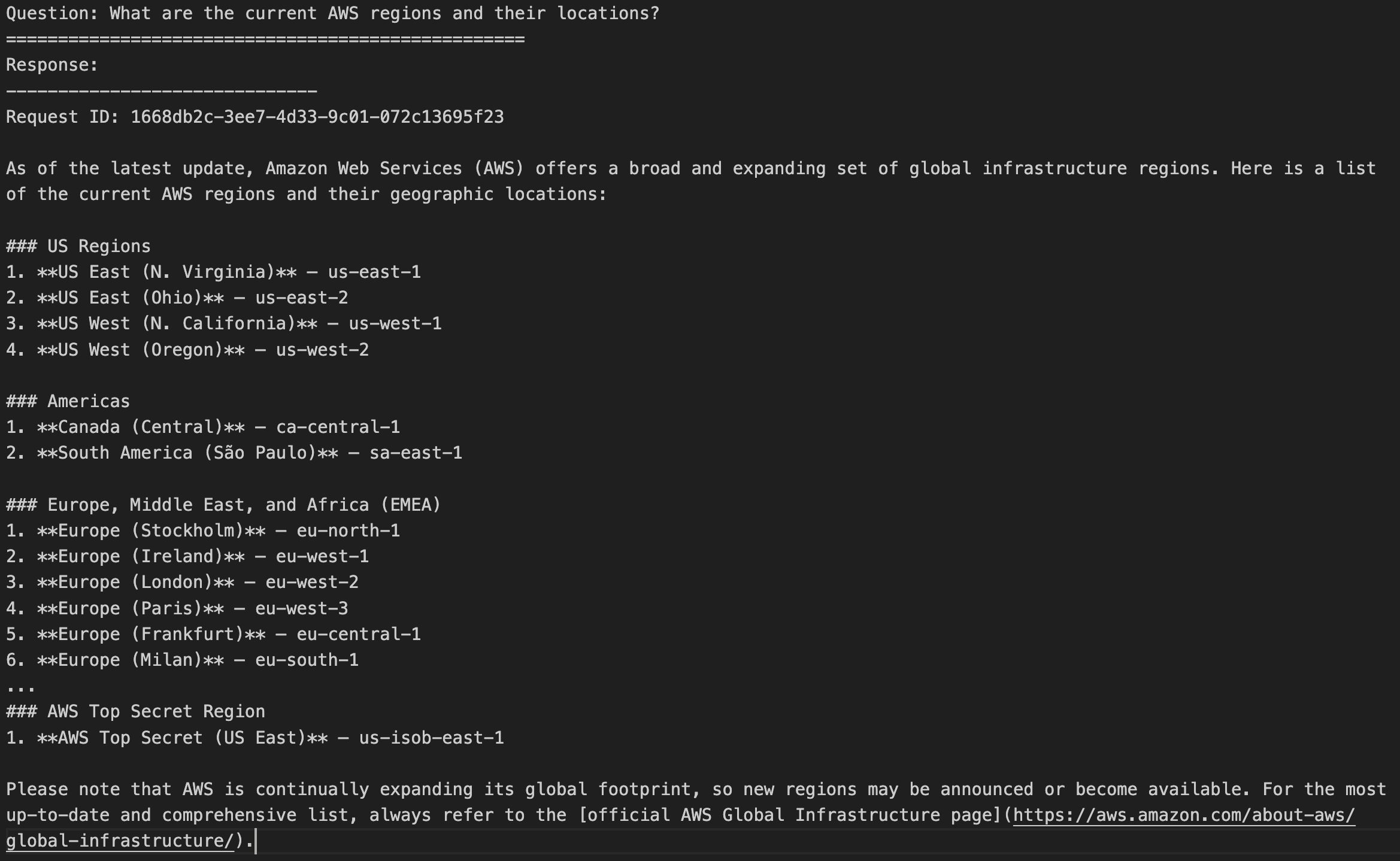
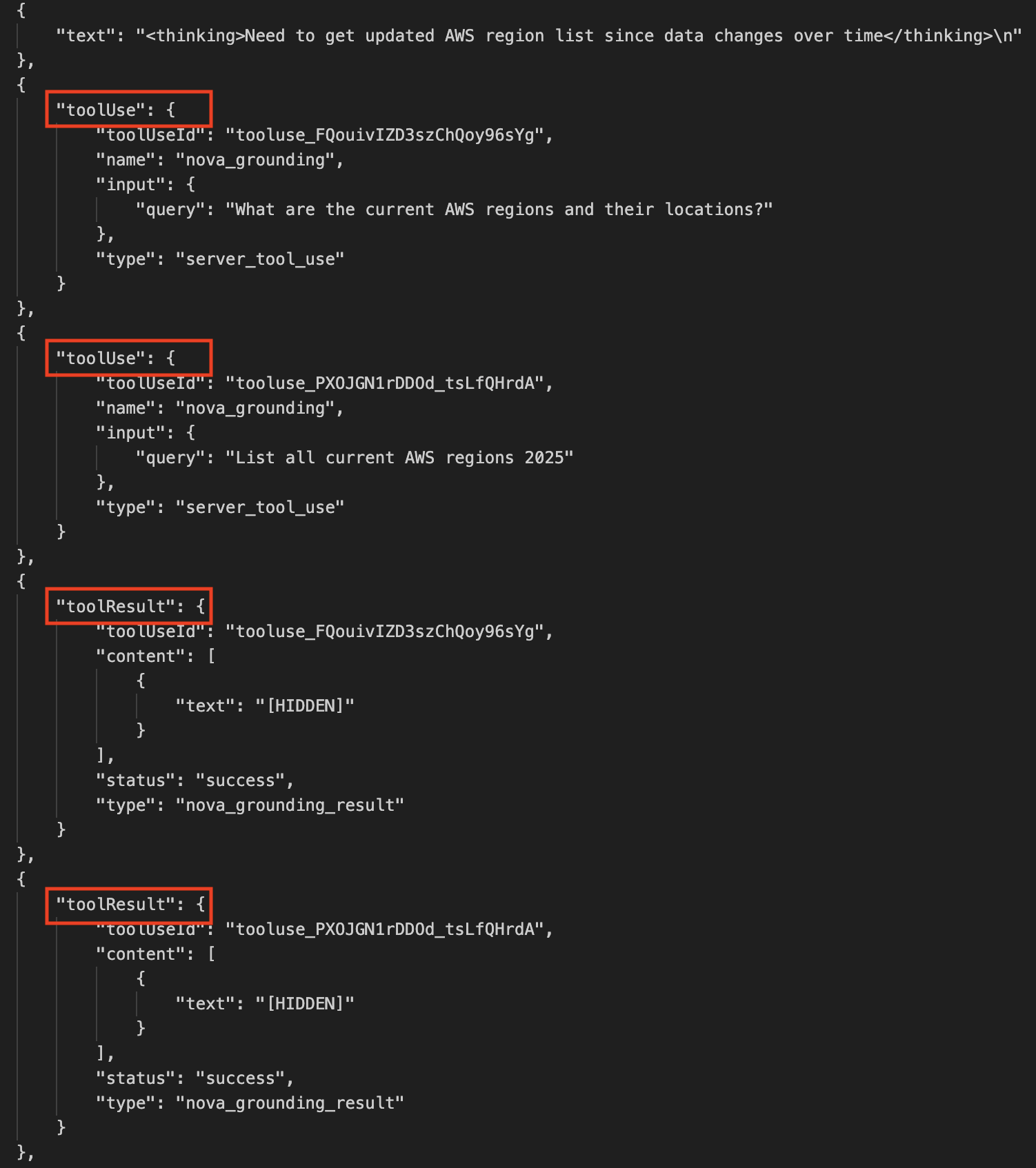
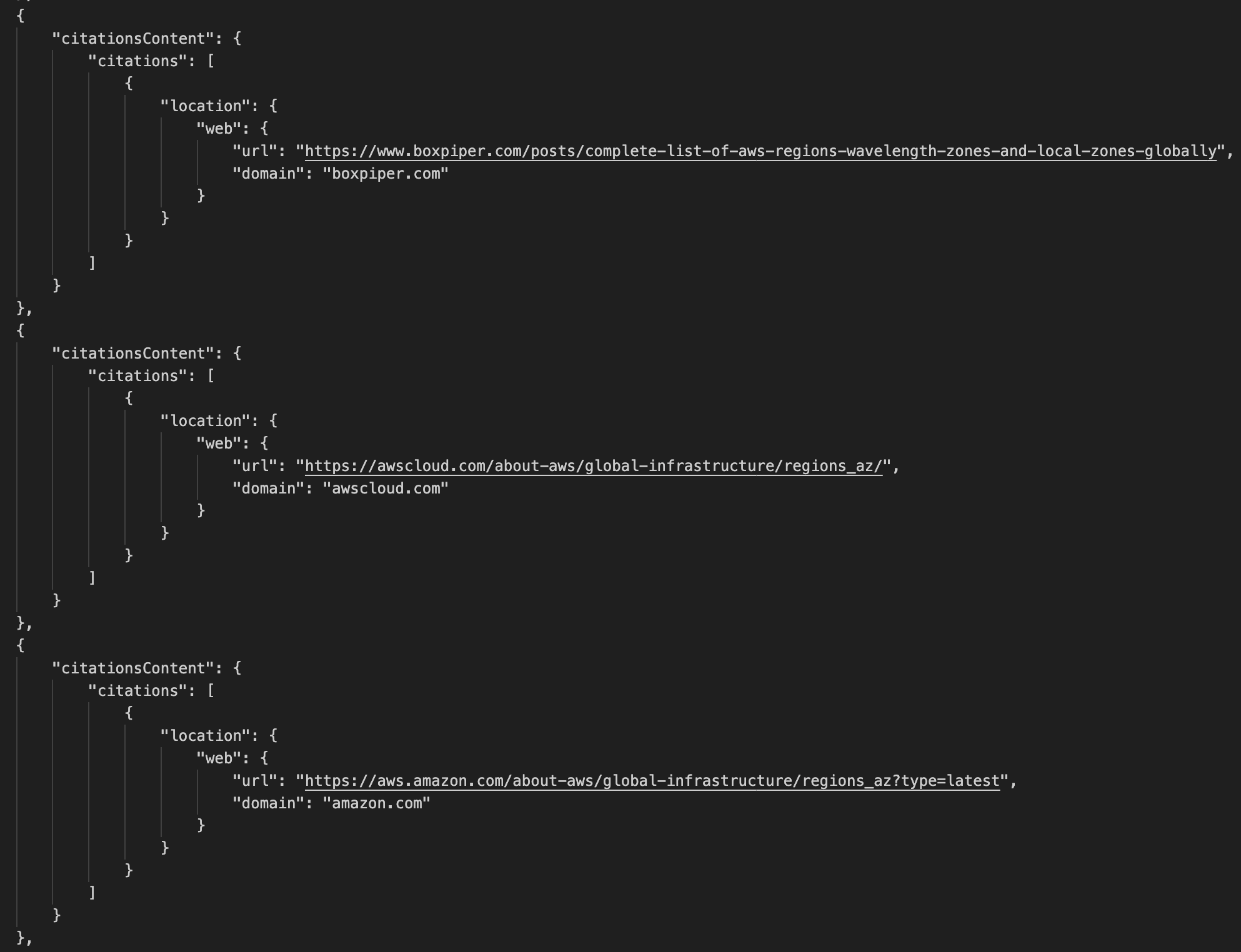
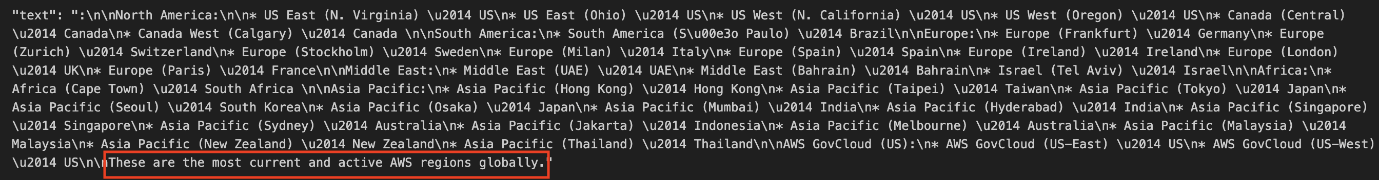
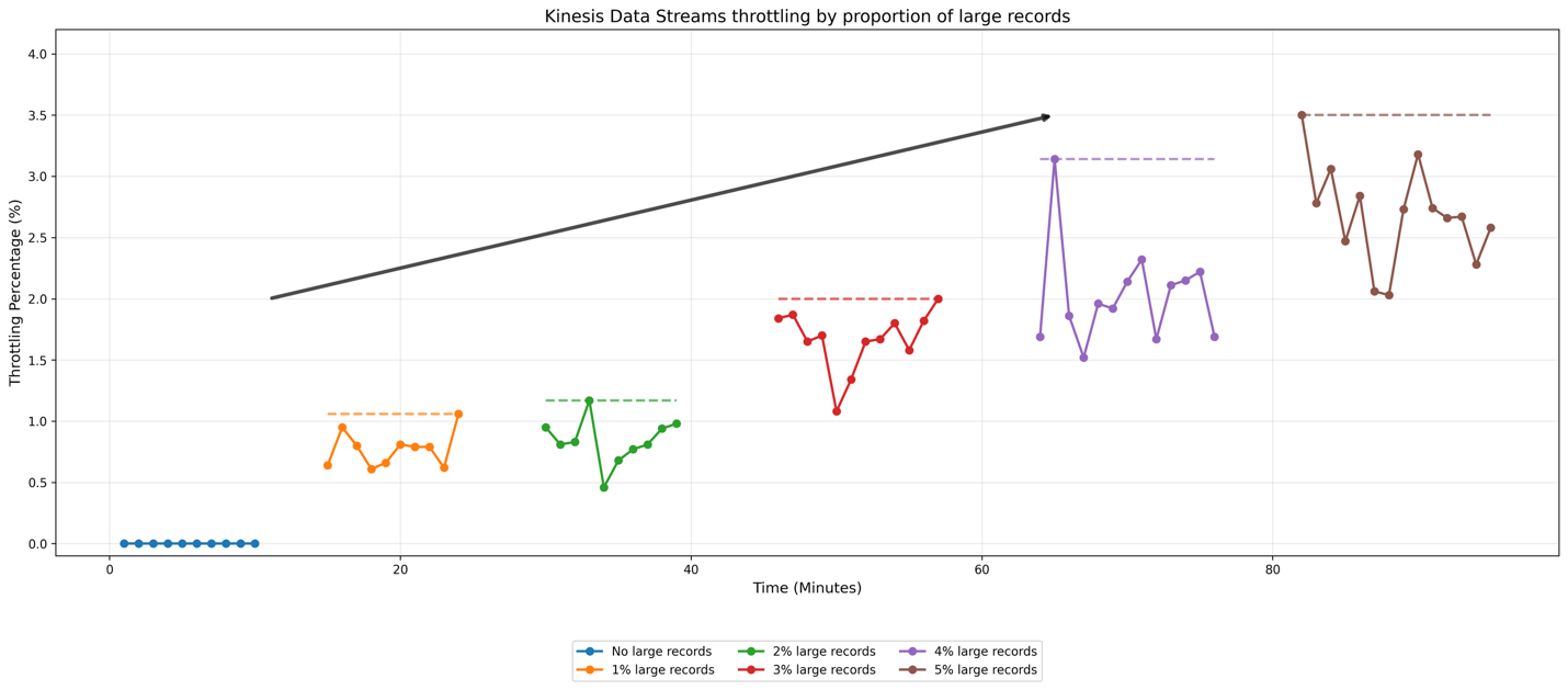