Post Syndicated from LastWeekTonight original https://www.youtube.com/shorts/sl9IRn33Fig
The Reliability Edge SREs Have Been Waiting For
Post Syndicated from Maddie Presland original https://www.backblaze.com/blog/the-reliability-edge-sres-have-been-waiting-for/

Site reliability engineers (SREs) are measured by one thing above all: keeping systems available when it matters most. They’re the ones getting calls at midnight, managing the war room during outages, and preventing small hiccups from snowballing into customer-facing failures.
But storage from major cloud providers often makes their job harder. Tiering delays stretch out recovery times. Replication gaps create blind spots across regions. Complex policy chains flood monitoring systems with noise. Instead of protecting reliability, general-purpose storage often undermines it.
What SREs need is a storage layer that works with them, not against them—one that delivers durability without complexity, speed without cold-tier delays, and clarity without policy sprawl.
A specialized, always-hot storage foundation provides exactly that.
This is the final post in our three-part series on how specialized storage helps every member of a cloud-native team. (See articles one and two to get the full story.) This time, we’re zeroing in on the reliability engineers who keep customer-facing systems humming behind the scenes.
Build a disaster recovery plan that’s ready for anything
Uncover proven frameworks for every stage of recovery and common pitfalls to avoid in our Essential Guide to Disaster Recovery Planning.
Reliability starts with storage
For SREs, storage is the backbone of availability and recovery. When it falters, the blast radius spreads fast. Even a minor failure can ripple outward and amplify the impact of every incident.
In the sections below, we’ll look at how those ripple effects play out in real-world scenarios, and how specialized, always-hot storage helps SREs contain failures, recover faster, and quiet the noise that makes reliability so hard to sustain.
Contain the blast radius
SREs spend much of their time running “what-if” drills. What if a drive fails? What if a region goes down? What if replication lags behind?
With general-purpose cloud storage, those “what-ifs” become real risks:
- Tiering delays: Infrequently accessed data is automatically pushed into colder, slower tiers. During an incident, archived data such as logs or snapshots must be restored before it’s usable. This slows recovery when seconds count.
- Replication gaps: Replication isn’t always immediate or consistent across regions. When writes lag or copies fall out of sync, recovery data can be stale or incomplete, leaving teams guessing at the true state of their systems.
- Policy complexity: Layers of identity and access management (IAM), lifecycle, and routing policies often overlap in unpredictable ways. A single misconfiguration—like archiving active data or blocking a needed API—can cascade through dependent services, turning a minor error into a wider outage.
Each layer meant to increase flexibility instead adds fragility.
Specialized storage changes that dynamic. Designed for worry-free durability and built to eliminate single points of failure, it distributes data across independent systems so localized issues don’t cascade. Even if hardware fails or a region experiences disruption, data remains accessible and recovery stays predictable. For SREs, that means fewer nightmare scenarios to model, fewer “what-ifs” in runbooks, and faster, more confident recovery.
Cut mean time to recovery (MTTR), protect SLAs
When an incident hits, the SLA clock starts ticking. Every minute spent waiting on logs, snapshots, or configs adds pressure from customers and leadership alike.
But in tiered storage systems, those critical assets are often parked in colder, low-cost tiers meant for archival access rather than fast recovery. Pulling them back can take hours or even days before triage can begin. That latency bloats MTTR and turns manageable events into prolonged outages with real customer impact.
Specialized storage eliminates these bottlenecks. Always-hot data and millisecond reads give SREs immediate visibility into logs, snapshots, and configs, so evidence is available the moment an incident begins. Instead of stalling while waiting on a restore job, teams can dive directly into diagnosis and resolution. The results are faster MTTR, steadier SLA performance, and fewer fire drills turning into headline outages.
Reduce alert fatigue
Ask any SRE what wears them down and the answer comes quickly: false alarms and 3 a.m. wake-ups. The incident itself may be rare, but the noise leading up to it is relentless.
In big-cloud environments, complexity breeds that noise:
- Lifecycle policies silently archive data until a request fails
- IAM rules misalign with pipeline needs
- Tier transitions or throttling events masquerade as outages in monitoring dashboards.
Each quirk becomes another alert, another call, another night interrupted. Over time, the noise blends with the signal, and teams start second-guessing what’s real. Alert fatigue sets in. Engineers tune out notifications or delay responses, not from neglect but from exhaustion. The result is a slower reaction when a real outage hits, which is exactly the scenario the alerts were meant to prevent.
Specialized storage dials down the chaos. A single-tier design with clear access controls strips away layers of risk, keeping alerts meaningful and edge cases rare. Instead of burning cycles firefighting brittle rules, SREs can focus on resilience engineering and prevent outages in the first place.
Rethink storage, strengthen reliability
The SRE role is already demanding. Storage shouldn’t add to the burden. An always-hot storage layer gives teams the durability, speed, and simplicity they need to keep systems reliable without extra toil.
Backblaze B2 was built with SREs in mind:
- Architected for 11 nine’s of durability
- Millisecond reads that slash MTTR and protect SLAs.
- Simplified architecture that cuts noise and pager fatigue.
You don’t need to rebuild your stack to get these benefits. Just swap the endpoint and redeploy. With Backblaze B2, storage stops undermining reliability and starts strengthening it.
Tired of midnight pages for preventable storage issues? There’s a better way. Explore how Backblaze B2 fits into your reliability workflows, and how much calmer on-call life feels when storage simply works.
The post The Reliability Edge SREs Have Been Waiting For appeared first on Backblaze Blog | Cloud Storage & Cloud Backup
[$] Fil-C: A memory-safe C implementation
Post Syndicated from daroc original https://lwn.net/Articles/1042938/
Fil-C is a memory-safe implementation of C and C++ that aims to let C code —
complete with pointer arithmetic, unions, and other features that are often
cited as a problem for memory-safe languages — run safely, unmodified.
Its dedication to being “fanatically
” makes it an attractive choice for retrofitting memory-safety
compatible
into existing applications. Despite the project’s relative youth and single
active contributor, Fil-C is capable of compiling an
entire memory-safe Linux user space (based on
Linux From Scratch),
albeit with some modifications to the more complex programs. It also features
memory-safe signal handling and a concurrent garbage collector.
The new home for Blockly
Post Syndicated from Philip Colligan, CBE original https://www.raspberrypi.org/blog/new-home-for-blockly/
I am delighted to announce that the Raspberry Pi Foundation is the new home for Blockly, the world’s leading open source library for visual programming.

What is Blockly?
Blockly is a free, open source library that enables developers to build applications and websites that use block-based coding interfaces. That means that instead of typing code, you snap blocks together to build programs. Behind the scenes, those blocks are turned into text-based code like JavaScript and Python.
Blockly started life in 2011 in Google as a passion project of one engineer. Since then — thanks to the generous support of Google, a small team of brilliant engineers, and an amazing community of open source contributors and partners — it has grown to become the de facto standard for visual programming interfaces.
In particular, Blockly is the foundation for pretty much all of the block-based coding applications that you may have used to teach or learn about programming. Platforms like Scratch, MakeCode, and MIT’s App Inventor are all built with Blockly. It’s no exaggeration to say that hundreds of millions of young people have learnt the fundamentals of computer science using software that is built with Blockly.

As we enter the age of AI, it is more important than ever that all young people develop a foundational understanding of computer science. Blockly and the block-based coding platforms and applications that it enables are essential to realising that vision.
You can read more about the importance of coding in the age of AI in our position paper.
Blockly is also widely used to create interfaces that control hardware and robotics platforms. And, while its main use cases are in education, Blockly is increasingly being used to build industrial and commercial applications.
What does this change mean?
From 10 November 2025, the Blockly open source library and assets, and key members of the Blockly team will transition from Google to the Raspberry Pi Foundation.
Our vision is for Blockly to continue to be the standard visual programming interface that makes coding accessible to all. We are committed to maintaining Blockly as an open source project, and to working collaboratively with the community of developers and educators.

Over the next year, we will roll out features that improve accessibility, including screen reader support and keyboard navigation, working closely with partners to support implementation of these accessibility improvements across their platforms.
Looking to the future, we want to make sure that Blockly is at the leading edge of innovations that support the teaching and learning of programming in the age of AI. We’re also excited about the potential for the Blockly team to collaborate with the Foundation’s research, learning, and product teams.
If you are already part of the community of developers and educators, then I want to reassure you that you can continue to expect the same outstanding partnership and support from the Blockly team. We also look forward to welcoming many more members to the Blockly community over the coming years.
Finally, I want to say a huge thank you to Google for their support for Blockly over the years, and for enabling this transition with generous grant funding.
The post The new home for Blockly appeared first on Raspberry Pi Foundation.
Broadway’s Buena Vista Social Club | Talks at Google
Post Syndicated from Talks at Google original https://www.youtube.com/watch?v=JwkEL0QAFFc
Amazon Nova Multimodal Embeddings: State-of-the-art embedding model for agentic RAG and semantic search
Post Syndicated from Danilo Poccia original https://aws.amazon.com/blogs/aws/amazon-nova-multimodal-embeddings-now-available-in-amazon-bedrock/
Today, we’re introducing Amazon Nova Multimodal Embeddings, a state-of-the-art multimodal embedding model for agentic retrieval-augmented generation (RAG) and semantic search applications, available in Amazon Bedrock. It is the first unified embedding model that supports text, documents, images, video, and audio through a single model to enable crossmodal retrieval with leading accuracy.
Embedding models convert textual, visual, and audio inputs into numerical representations called embeddings. These embeddings capture the meaning of the input in a way that AI systems can compare, search, and analyze, powering use cases such as semantic search and RAG.
Organizations are increasingly seeking solutions to unlock insights from the growing volume of unstructured data that is spread across text, image, document, video, and audio content. For example, an organization might have product images, brochures that contain infographics and text, and user-uploaded video clips. Embedding models are able to unlock value from unstructured data, however traditional models are typically specialized to handle one content type. This limitation drives customers to either build complex crossmodal embedding solutions or restrict themselves to use cases focused on a single content type. The problem also applies to mixed-modality content types such as documents with interleaved text and images or video with visual, audio, and textual elements where existing models struggle to capture crossmodal relationships effectively.
Nova Multimodal Embeddings supports a unified semantic space for text, documents, images, video, and audio for use cases such as crossmodal search across mixed-modality content, searching with a reference image, and retrieving visual documents.
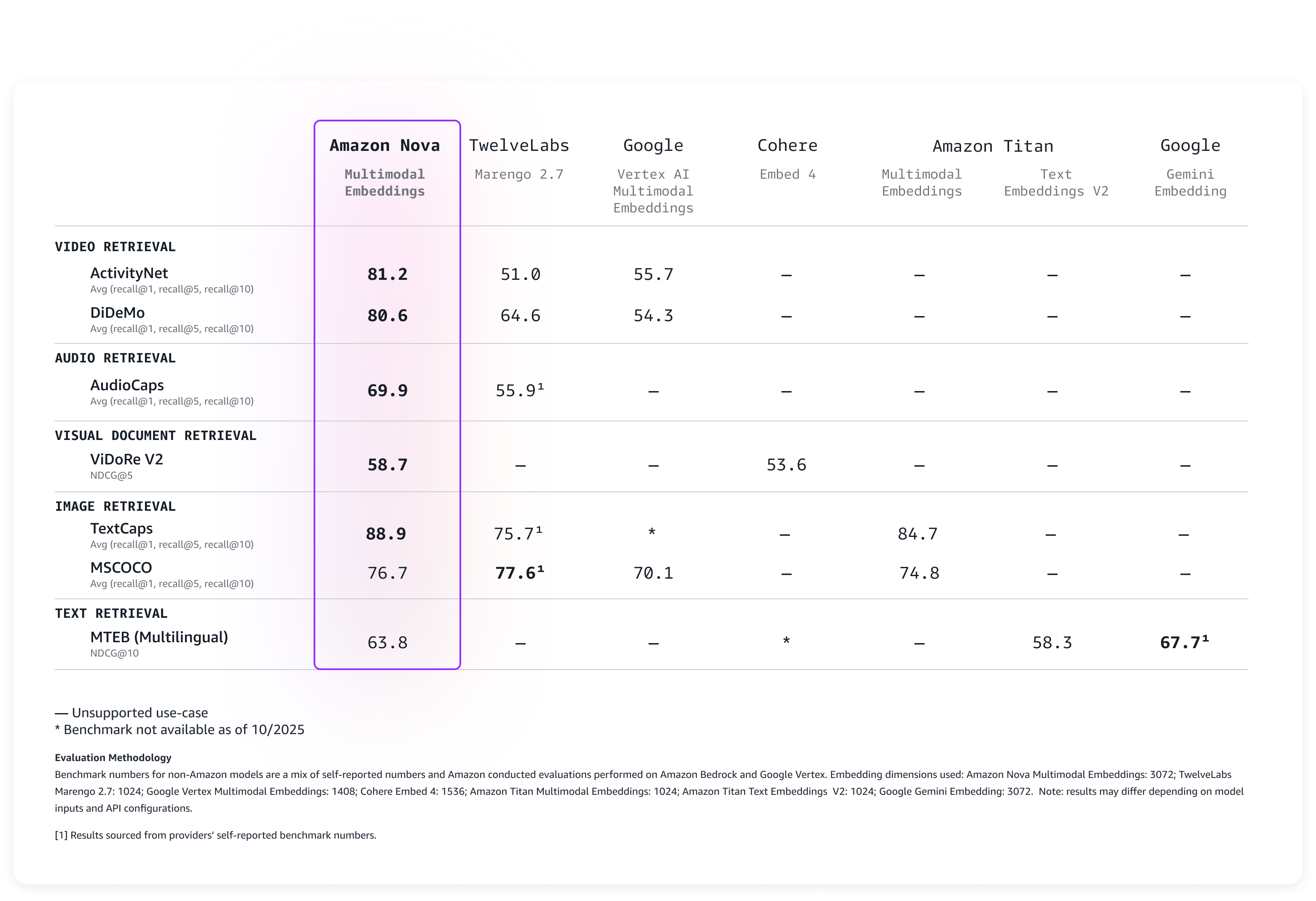
Evaluating Amazon Nova Multimodal Embeddings performance
We evaluated the model on a broad range of benchmarks, and it delivers leading accuracy out-of-the-box as described in the following table.
Nova Multimodal Embeddings supports a context length of up to 8K tokens, text in up to 200 languages, and accepts inputs via synchronous and asynchronous APIs. Additionally, it supports segmentation (also known as “chunking”) to partition long-form text, video, or audio content into manageable segments, generating embeddings for each portion. Lastly, the model offers four output embedding dimensions, trained using Matryoshka Representation Learning (MRL) that enables low-latency end-to-end retrieval with minimal accuracy changes.
Let’s see how the new model can be used in practice.
Using Amazon Nova Multimodal Embeddings
Getting started with Nova Multimodal Embeddings follows the same pattern as other models in Amazon Bedrock. The model accepts text, documents, images, video, or audio as input and returns numerical embeddings that you can use for semantic search, similarity comparison, or RAG.
Here’s a practical example using the AWS SDK for Python (Boto3) that shows how to create embeddings from different content types and store them for later retrieval. For simplicity, I’ll use Amazon S3 Vectors, a cost-optimized storage with native support for storing and querying vectors at any scale, to store and search the embeddings.
Let’s start with the fundamentals: converting text into embeddings. This example shows how to transform a simple text description into a numerical representation that captures its semantic meaning. These embeddings can later be compared with embeddings from documents, images, videos, or audio to find related content.
To make the code easy to follow, I’ll show a section of the script at a time. The full script is included at the end of this walkthrough.
import json
import base64
import time
import boto3

MODEL_ID = "amazon.nova-2-multimodal-embeddings-v1:0"
EMBEDDING_DIMENSION = 3072

# Initialize Amazon Bedrock Runtime client
bedrock_runtime = boto3.client("bedrock-runtime", region_name="us-east-1")

print(f"Generating text embedding with {MODEL_ID} ...")

# Text to embed
text = "Amazon Nova is a multimodal foundation model"

# Create embedding
request_body = {
    "taskType": "SINGLE_EMBEDDING",
    "singleEmbeddingParams": {
        "embeddingPurpose": "GENERIC_INDEX",
        "embeddingDimension": EMBEDDING_DIMENSION,
        "text": {"truncationMode": "END", "value": text},
    },
}

response = bedrock_runtime.invoke_model(
    body=json.dumps(request_body),
    modelId=MODEL_ID,
    contentType="application/json",
)

# Extract embedding
response_body = json.loads(response["body"].read())
embedding = response_body["embeddings"][0]["embedding"]

print(f"Generated embedding with {len(embedding)} dimensions")
Now we’ll process visual content using the same embedding space using a photo.jpg file in the same folder as the script. This demonstrates the power of multimodality: Nova Multimodal Embeddings is able to capture both textual and visual context into a single embedding that provides enhanced understanding of the document.
Nova Multimodal Embeddings can generate embeddings that are optimized for how they are being used. When indexing for a search or retrieval use case, embeddingPurpose can be set to GENERIC_INDEX. For the query step, embeddingPurpose can be set depending on the type of item to be retrieved. For example, when retrieving documents, embeddingPurpose can be set to DOCUMENT_RETRIEVAL.
# Read and encode image
print(f"Generating image embedding with {MODEL_ID} ...")

with open("photo.jpg", "rb") as f:
    image_bytes = base64.b64encode(f.read()).decode("utf-8")

# Create embedding
request_body = {
    "taskType": "SINGLE_EMBEDDING",
    "singleEmbeddingParams": {
        "embeddingPurpose": "GENERIC_INDEX",
        "embeddingDimension": EMBEDDING_DIMENSION,
        "image": {
            "format": "jpeg",
            "source": {"bytes": image_bytes}
        },
    },
}

response = bedrock_runtime.invoke_model(
    body=json.dumps(request_body),
    modelId=MODEL_ID,
    contentType="application/json",
)

# Extract embedding
response_body = json.loads(response["body"].read())
embedding = response_body["embeddings"][0]["embedding"]

print(f"Generated embedding with {len(embedding)} dimensions")
To process video content, I use the asynchronous API. That’s a requirement for videos that are larger than 25MB when encoded as Base64. First, I upload a local video to an S3 bucket in the same AWS Region.
aws s3 cp presentation.mp4 s3://my-video-bucket/videos/This example shows how to extract embeddings from both visual and audio components of a video file. The segmentation feature breaks longer videos into manageable chunks, making it practical to search through hours of content efficiently.
# Initialize Amazon S3 client
s3 = boto3.client("s3", region_name="us-east-1")

print(f"Generating video embedding with {MODEL_ID} ...")

# Amazon S3 URIs
S3_VIDEO_URI = "s3://my-video-bucket/videos/presentation.mp4"
S3_EMBEDDING_DESTINATION_URI = "s3://my-embedding-destination-bucket/embeddings-output/"

# Create async embedding job for video with audio
model_input = {
    "taskType": "SEGMENTED_EMBEDDING",
    "segmentedEmbeddingParams": {
        "embeddingPurpose": "GENERIC_INDEX",
        "embeddingDimension": EMBEDDING_DIMENSION,
        "video": {
            "format": "mp4",
            "embeddingMode": "AUDIO_VIDEO_COMBINED",
            "source": {
                "s3Location": {"uri": S3_VIDEO_URI}
            },
            "segmentationConfig": {
                "durationSeconds": 15  # Segment into 15-second chunks
            },
        },
    },
}

response = bedrock_runtime.start_async_invoke(
    modelId=MODEL_ID,
    modelInput=model_input,
    outputDataConfig={
        "s3OutputDataConfig": {
            "s3Uri": S3_EMBEDDING_DESTINATION_URI
        }
    },
)

invocation_arn = response["invocationArn"]
print(f"Async job started: {invocation_arn}")

# Poll until job completes
print("\nPolling for job completion...")
while True:
    job = bedrock_runtime.get_async_invoke(invocationArn=invocation_arn)
    status = job["status"]
    print(f"Status: {status}")

    if status != "InProgress":
        break
    time.sleep(15)

# Check if job completed successfully
if status == "Completed":
    output_s3_uri = job["outputDataConfig"]["s3OutputDataConfig"]["s3Uri"]
    print(f"\nSuccess! Embeddings at: {output_s3_uri}")

    # Parse S3 URI to get bucket and prefix
    s3_uri_parts = output_s3_uri[5:].split("/", 1)  # Remove "s3://" prefix
    bucket = s3_uri_parts[0]
    prefix = s3_uri_parts[1] if len(s3_uri_parts) > 1 else ""

    # AUDIO_VIDEO_COMBINED mode outputs to embedding-audio-video.jsonl
    # The output_s3_uri already includes the job ID, so just append the filename
    embeddings_key = f"{prefix}/embedding-audio-video.jsonl".lstrip("/")

    print(f"Reading embeddings from: s3://{bucket}/{embeddings_key}")

    # Read and parse JSONL file
    response = s3.get_object(Bucket=bucket, Key=embeddings_key)
    content = response['Body'].read().decode('utf-8')

    embeddings = []
    for line in content.strip().split('\n'):
        if line:
            embeddings.append(json.loads(line))

    print(f"\nFound {len(embeddings)} video segments:")
    for i, segment in enumerate(embeddings):
        print(f"  Segment {i}: {segment.get('startTime', 0):.1f}s - {segment.get('endTime', 0):.1f}s")
        print(f"    Embedding dimension: {len(segment.get('embedding', []))}")
else:
    print(f"\nJob failed: {job.get('failureMessage', 'Unknown error')}")
With our embeddings generated, we need a place to store and search them efficiently. This example demonstrates setting up a vector store using Amazon S3 Vectors, which provides the infrastructure needed for similarity search at scale. Think of this as creating a searchable index where semantically similar content naturally clusters together. When adding an embedding to the index, I use the metadata to specify the original format and the content being indexed.
# Initialize Amazon S3 Vectors client
s3vectors = boto3.client("s3vectors", region_name="us-east-1")

# Configuration
VECTOR_BUCKET = "my-vector-store"
INDEX_NAME = "embeddings"

# Create vector bucket and index (if they don't exist)
try:
    s3vectors.get_vector_bucket(vectorBucketName=VECTOR_BUCKET)
    print(f"Vector bucket {VECTOR_BUCKET} already exists")
except s3vectors.exceptions.NotFoundException:
    s3vectors.create_vector_bucket(vectorBucketName=VECTOR_BUCKET)
    print(f"Created vector bucket: {VECTOR_BUCKET}")

try:
    s3vectors.get_index(vectorBucketName=VECTOR_BUCKET, indexName=INDEX_NAME)
    print(f"Vector index {INDEX_NAME} already exists")
except s3vectors.exceptions.NotFoundException:
    s3vectors.create_index(
        vectorBucketName=VECTOR_BUCKET,
        indexName=INDEX_NAME,
        dimension=EMBEDDING_DIMENSION,
        dataType="float32",
        distanceMetric="cosine"
    )
    print(f"Created index: {INDEX_NAME}")

texts = [
    "Machine learning on AWS",
    "Amazon Bedrock provides foundation models",
    "S3 Vectors enables semantic search"
]

print(f"\nGenerating embeddings for {len(texts)} texts...")

# Generate embeddings using Amazon Nova for each text
vectors = []
for text in texts:
    response = bedrock_runtime.invoke_model(
        body=json.dumps({
            "taskType": "SINGLE_EMBEDDING",
            "singleEmbeddingParams": {
                "embeddingDimension": EMBEDDING_DIMENSION,
                "text": {"truncationMode": "END", "value": text}
            }
        }),
        modelId=MODEL_ID,
        accept="application/json",
        contentType="application/json"
    )

    response_body = json.loads(response["body"].read())
    embedding = response_body["embeddings"][0]["embedding"]

    vectors.append({
        "key": f"text:{text[:50]}",  # Unique identifier
        "data": {"float32": embedding},
        "metadata": {"type": "text", "content": text}
    })
    print(f"  ✓ Generated embedding for: {text}")

# Add all vectors to store in a single call
s3vectors.put_vectors(
    vectorBucketName=VECTOR_BUCKET,
    indexName=INDEX_NAME,
    vectors=vectors
)

print(f"\nSuccessfully added {len(vectors)} vectors to the store in one put_vectors call!")
This final example demonstrates the capability of searching across different content types with a single query, finding the most similar content regardless of whether it originated from text, images, videos, or audio. The distance scores help you understand how closely related the results are to your original query.
# Text to query
query_text = "foundation models"

print(f"\nGenerating embeddings for query '{query_text}' ...")

# Generate embeddings
response = bedrock_runtime.invoke_model(
    body=json.dumps({
        "taskType": "SINGLE_EMBEDDING",
        "singleEmbeddingParams": {
            "embeddingPurpose": "GENERIC_RETRIEVAL",
            "embeddingDimension": EMBEDDING_DIMENSION,
            "text": {"truncationMode": "END", "value": query_text}
        }
    }),
    modelId=MODEL_ID,
    accept="application/json",
    contentType="application/json"
)

response_body = json.loads(response["body"].read())
query_embedding = response_body["embeddings"][0]["embedding"]

print(f"Searching for similar embeddings...\n")

# Search for top 5 most similar vectors
response = s3vectors.query_vectors(
    vectorBucketName=VECTOR_BUCKET,
    indexName=INDEX_NAME,
    queryVector={"float32": query_embedding},
    topK=5,
    returnDistance=True,
    returnMetadata=True
)

# Display results
print(f"Found {len(response['vectors'])} results:\n")
for i, result in enumerate(response["vectors"], 1):
    print(f"{i}. {result['key']}")
    print(f"   Distance: {result['distance']:.4f}")
    if result.get("metadata"):
        print(f"   Metadata: {result['metadata']}")
    print()
Crossmodal search is one of the key advantages of multimodal embeddings. With crossmodal search, you can query with text and find relevant images. You can also search for videos using text descriptions, find audio clips that match certain topics, or discover documents based on their visual and textual content. For your reference, the full script with all previous examples merged together is here:
import json
import base64
import time
import boto3

MODEL_ID = "amazon.nova-2-multimodal-embeddings-v1:0"
EMBEDDING_DIMENSION = 3072

# Initialize Amazon Bedrock Runtime client
bedrock_runtime = boto3.client("bedrock-runtime", region_name="us-east-1")

print(f"Generating text embedding with {MODEL_ID} ...")

# Text to embed
text = "Amazon Nova is a multimodal foundation model"

# Create embedding
request_body = {
    "taskType": "SINGLE_EMBEDDING",
    "singleEmbeddingParams": {
        "embeddingPurpose": "GENERIC_INDEX",
        "embeddingDimension": EMBEDDING_DIMENSION,
        "text": {"truncationMode": "END", "value": text},
    },
}

response = bedrock_runtime.invoke_model(
    body=json.dumps(request_body),
    modelId=MODEL_ID,
    contentType="application/json",
)

# Extract embedding
response_body = json.loads(response["body"].read())
embedding = response_body["embeddings"][0]["embedding"]

print(f"Generated embedding with {len(embedding)} dimensions")
# Read and encode image
print(f"Generating image embedding with {MODEL_ID} ...")

with open("photo.jpg", "rb") as f:
    image_bytes = base64.b64encode(f.read()).decode("utf-8")

# Create embedding
request_body = {
    "taskType": "SINGLE_EMBEDDING",
    "singleEmbeddingParams": {
        "embeddingPurpose": "GENERIC_INDEX",
        "embeddingDimension": EMBEDDING_DIMENSION,
        "image": {
            "format": "jpeg",
            "source": {"bytes": image_bytes}
        },
    },
}

response = bedrock_runtime.invoke_model(
    body=json.dumps(request_body),
    modelId=MODEL_ID,
    contentType="application/json",
)

# Extract embedding
response_body = json.loads(response["body"].read())
embedding = response_body["embeddings"][0]["embedding"]

print(f"Generated embedding with {len(embedding)} dimensions")
# Initialize Amazon S3 client
s3 = boto3.client("s3", region_name="us-east-1")

print(f"Generating video embedding with {MODEL_ID} ...")

# Amazon S3 URIs
S3_VIDEO_URI = "s3://my-video-bucket/videos/presentation.mp4"

# Amazon S3 output bucket and location
S3_EMBEDDING_DESTINATION_URI = "s3://my-video-bucket/embeddings-output/"

# Create async embedding job for video with audio
model_input = {
    "taskType": "SEGMENTED_EMBEDDING",
    "segmentedEmbeddingParams": {
        "embeddingPurpose": "GENERIC_INDEX",
        "embeddingDimension": EMBEDDING_DIMENSION,
        "video": {
            "format": "mp4",
            "embeddingMode": "AUDIO_VIDEO_COMBINED",
            "source": {
                "s3Location": {"uri": S3_VIDEO_URI}
            },
            "segmentationConfig": {
                "durationSeconds": 15  # Segment into 15-second chunks
            },
        },
    },
}

response = bedrock_runtime.start_async_invoke(
    modelId=MODEL_ID,
    modelInput=model_input,
    outputDataConfig={
        "s3OutputDataConfig": {
            "s3Uri": S3_EMBEDDING_DESTINATION_URI
        }
    },
)

invocation_arn = response["invocationArn"]
print(f"Async job started: {invocation_arn}")

# Poll until job completes
print("\nPolling for job completion...")
while True:
    job = bedrock_runtime.get_async_invoke(invocationArn=invocation_arn)
    status = job["status"]
    print(f"Status: {status}")

    if status != "InProgress":
        break
    time.sleep(15)

# Check if job completed successfully
if status == "Completed":
    output_s3_uri = job["outputDataConfig"]["s3OutputDataConfig"]["s3Uri"]
    print(f"\nSuccess! Embeddings at: {output_s3_uri}")

    # Parse S3 URI to get bucket and prefix
    s3_uri_parts = output_s3_uri[5:].split("/", 1)  # Remove "s3://" prefix
    bucket = s3_uri_parts[0]
    prefix = s3_uri_parts[1] if len(s3_uri_parts) > 1 else ""

    # AUDIO_VIDEO_COMBINED mode outputs to embedding-audio-video.jsonl
    # The output_s3_uri already includes the job ID, so just append the filename
    embeddings_key = f"{prefix}/embedding-audio-video.jsonl".lstrip("/")

    print(f"Reading embeddings from: s3://{bucket}/{embeddings_key}")

    # Read and parse JSONL file
    response = s3.get_object(Bucket=bucket, Key=embeddings_key)
    content = response['Body'].read().decode('utf-8')

    embeddings = []
    for line in content.strip().split('\n'):
        if line:
            embeddings.append(json.loads(line))

    print(f"\nFound {len(embeddings)} video segments:")
    for i, segment in enumerate(embeddings):
        print(f"  Segment {i}: {segment.get('startTime', 0):.1f}s - {segment.get('endTime', 0):.1f}s")
        print(f"    Embedding dimension: {len(segment.get('embedding', []))}")
else:
    print(f"\nJob failed: {job.get('failureMessage', 'Unknown error')}")
# Initialize Amazon S3 Vectors client
s3vectors = boto3.client("s3vectors", region_name="us-east-1")

# Configuration
VECTOR_BUCKET = "my-vector-store"
INDEX_NAME = "embeddings"

# Create vector bucket and index (if they don't exist)
try:
    s3vectors.get_vector_bucket(vectorBucketName=VECTOR_BUCKET)
    print(f"Vector bucket {VECTOR_BUCKET} already exists")
except s3vectors.exceptions.NotFoundException:
    s3vectors.create_vector_bucket(vectorBucketName=VECTOR_BUCKET)
    print(f"Created vector bucket: {VECTOR_BUCKET}")

try:
    s3vectors.get_index(vectorBucketName=VECTOR_BUCKET, indexName=INDEX_NAME)
    print(f"Vector index {INDEX_NAME} already exists")
except s3vectors.exceptions.NotFoundException:
    s3vectors.create_index(
        vectorBucketName=VECTOR_BUCKET,
        indexName=INDEX_NAME,
        dimension=EMBEDDING_DIMENSION,
        dataType="float32",
        distanceMetric="cosine"
    )
    print(f"Created index: {INDEX_NAME}")

texts = [
    "Machine learning on AWS",
    "Amazon Bedrock provides foundation models",
    "S3 Vectors enables semantic search"
]

print(f"\nGenerating embeddings for {len(texts)} texts...")

# Generate embeddings using Amazon Nova for each text
vectors = []
for text in texts:
    response = bedrock_runtime.invoke_model(
        body=json.dumps({
            "taskType": "SINGLE_EMBEDDING",
            "singleEmbeddingParams": {
                "embeddingPurpose": "GENERIC_INDEX",
                "embeddingDimension": EMBEDDING_DIMENSION,
                "text": {"truncationMode": "END", "value": text}
            }
        }),
        modelId=MODEL_ID,
        accept="application/json",
        contentType="application/json"
    )

    response_body = json.loads(response["body"].read())
    embedding = response_body["embeddings"][0]["embedding"]

    vectors.append({
        "key": f"text:{text[:50]}",  # Unique identifier
        "data": {"float32": embedding},
        "metadata": {"type": "text", "content": text}
    })
    print(f"  ✓ Generated embedding for: {text}")

# Add all vectors to store in a single call
s3vectors.put_vectors(
    vectorBucketName=VECTOR_BUCKET,
    indexName=INDEX_NAME,
    vectors=vectors
)

print(f"\nSuccessfully added {len(vectors)} vectors to the store in one put_vectors call!")
# Text to query
query_text = "foundation models"

print(f"\nGenerating embeddings for query '{query_text}' ...")

# Generate embeddings
response = bedrock_runtime.invoke_model(
    body=json.dumps({
        "taskType": "SINGLE_EMBEDDING",
        "singleEmbeddingParams": {
            "embeddingPurpose": "GENERIC_RETRIEVAL",
            "embeddingDimension": EMBEDDING_DIMENSION,
            "text": {"truncationMode": "END", "value": query_text}
        }
    }),
    modelId=MODEL_ID,
    accept="application/json",
    contentType="application/json"
)

response_body = json.loads(response["body"].read())
query_embedding = response_body["embeddings"][0]["embedding"]

print(f"Searching for similar embeddings...\n")

# Search for top 5 most similar vectors
response = s3vectors.query_vectors(
    vectorBucketName=VECTOR_BUCKET,
    indexName=INDEX_NAME,
    queryVector={"float32": query_embedding},
    topK=5,
    returnDistance=True,
    returnMetadata=True
)

# Display results
print(f"Found {len(response['vectors'])} results:\n")
for i, result in enumerate(response["vectors"], 1):
    print(f"{i}. {result['key']}")
    print(f"   Distance: {result['distance']:.4f}")
    if result.get("metadata"):
        print(f"   Metadata: {result['metadata']}")
    print()
For production applications, embeddings can be stored in any vector database. Amazon OpenSearch Service offers native integration with Nova Multimodal Embeddings at launch, making it straightforward to build scalable search applications. As shown in the examples before, Amazon S3 Vectors provides a simple way to store and query embeddings with your application data.
Things to know
Nova Multimodal Embeddings offers four output dimension options: 3,072, 1,024, 384, and 256. Larger dimensions provide more detailed representations but require more storage and computation. Smaller dimensions offer a practical balance between retrieval performance and resource efficiency. This flexibility helps you optimize for your specific application and cost requirements.
The model handles substantial context lengths. For text inputs, it can process up to 8,192 tokens at once. Video and audio inputs support segments of up to 30 seconds, and the model can segment longer files. This segmentation capability is particularly useful when working with large media files—the model splits them into manageable pieces and creates embeddings for each segment.
The model includes responsible AI features built into Amazon Bedrock. Content submitted for embedding goes through Amazon Bedrock content safety filters, and the model includes fairness measures to reduce bias.
As described in the code examples, the model can be invoked through both synchronous and asynchronous APIs. The synchronous API works well for real-time applications where you need immediate responses, such as processing user queries in a search interface. The asynchronous API handles latency insensitive workloads more efficiently, making it suitable for processing large content such as videos.
Availability and pricing
Amazon Nova Multimodal Embeddings is available today in Amazon Bedrock in the US East (N. Virginia) AWS Region. For detailed pricing information, visit the Amazon Bedrock pricing page.
To learn more, see the Amazon Nova User Guide for comprehensive documentation and the Amazon Nova model cookbook on GitHub for practical code examples.
If you’re using an AI–powered assistant for software development such as Amazon Q Developer or Kiro, you can set up the AWS API MCP Server to help the AI assistants interact with AWS services and resources and the AWS Knowledge MCP Server to provide up-to-date documentation, code samples, knowledge about the regional availability of AWS APIs and CloudFormation resources.
Start building multimodal AI-powered applications with Nova Multimodal Embeddings today, and share your feedback through AWS re:Post for Amazon Bedrock or your usual AWS Support contacts.
— Danilo
Fedora Linux 43 released (Fedora Magazine)
Post Syndicated from jzb original https://lwn.net/Articles/1043785/
The Fedora Project has announced the release of Fedora Linux 43,
with “what’s new” articles for Fedora
Workstation, Fedora
KDE Plasma Desktop, and Fedora
Atomic Desktops.
For those of you installing fresh Fedora Linux 43 Spins, you may be
greeted with the new Anaconda WebUI. This was the default installer
interface for Fedora Workstation 42, and now it’s the default
installer UI for the Spins as well.If you are a GNOME desktop user, you’ll also notice that the GNOME
is now Wayland-only in Fedora Linux 43. GNOME upstream has deprecated
X11 support, and has disabled it as a compile time default in GNOME 49. Upstream GNOME plans to fully remove X11 support in GNOME 50.
See the release
notes for a full list of changes in Fedora 43.
Monitoring MDM Certificates with Lab9 Pro and Zabbix
Post Syndicated from Michael Kammer original https://blog.zabbix.com/monitoring-mdm-certificates-with-lab9-pro-and-zabbix/31621/

Lab9 Pro is the B2B division of Lab9, Belgium’s leading Apple Premium Partner. With over 30 years of experience, Lab9 Pro specializes in integrating and supporting Apple systems within businesses, educational institutions, and public organizations. Beyond Apple expertise, Lab9 Pro also designs, implements, and maintains complete IT infrastructures, including networks, servers, storage, and security solutions.
The challenge
It’s impossible to manage devices at organizations without the use of a good MDM (Mobile Device Management) system such as Jamf. As the leading provider of Apple device management solutions, Jamf empowers organizations to deploy, manage, and secure Apple devices at scale.
Even in smaller organizations Jamf is the right solution, as small and medium-sized enterprises (SMEs) often lack the resources to manage their MDM systems. Offering an MSP model solves a lot of problems for these customers.
For Apple device management, the typical customer has a few certificates issued by Apple, which require approval of the user agreement by the Apple business or school manager. Without getting too technical about Apple Device management, depending on the customer the certificates need to be renewed on different dates. If the user agreement is not approved, automated device enrollment will stop working.
Lab9 Pro found themselves needing to check all certificates and user agreements for MSP customers manually, which involved an unacceptably high error rate that often caused discontinuity of the MDM system.
The solution
Lab9 Pro were already using Zabbix to monitor customer environments and their own infrastructure, including storage, firewalls, switches, and more. Because Zabbix offers a wide variety of options that make it possible to monitor almost anything, it was only logical to explore whether Zabbix could also be used to monitor the MDM certificates.
The research phase
Step one was to check the availability of certificate information. Unfortunately, Apple Business Manager’s API did not help much, as it does not provide certificate details. Instead, the team at Lab9 Pro investigated the Jamf API.
Although it doesn’t directly return certificate information either, they found something even more useful – Jamf’s API provides customer instance notifications. These include alerts when certificates (VPP, PUSH, DEP, etc.) are about to expire (typically 10 days in advance) as well as when the Device Enrollment Program (user agreement) is not approved.
Zabbix implementation
Since Lab9 Pro manages multiple MSP tenants, they created a dedicated Zabbix template. This template includes both pre-filled and empty macros:
Pre-filled macros:
• {$JAMF.AUTH.INTERVAL}: Interval for retrieving the bearer token
• {$JAMF.NOTIF.INTERVAL}: Interval for retrieving Jamf notifications
• {$JAMF.PATH.AUTH}: API path for retrieving the bearer token
• {$JAMF.PATH.NOTIFICATIONS}: API path for retrieving Jamf notifications
Empty macros:
• {$JAMF.URL}: Jamf URL
• {$JAMF.API.USER}: Jamf user account for authentication
• {$JAMF.API.PASSWORD}: Jamf password (stored as a secret value)
The team configured an item to perform an API call to retrieve the bearer token. A preprocessing rule in JavaScript stores this token in a variable. Discovery rules proved very useful for executing API calls to retrieve Jamf notifications using the bearer token. This was achieved by configuring preprocessing steps and Low-Level Discovery (LLD) macros to pass the Jamf URL and bearer token. Trigger prototypes for each certificate were also added within the same discovery rule.
The results
Whenever a certificate is nearing expiration, a problem is automatically displayed on Lab9 Pro’s Zabbix dashboard, which is visible on TV screens placed throughout their office in order to make sure the entire team is aware of upcoming certificate renewals.
Since Lab9 Pro began monitoring MDM certificates through the Jamf API, they have experienced zero expired certificates, which in turn has allowed them to avoid situations where devices become unmanaged and require a full setup again.
Zabbix makes it possible for Lab9 Pro to keep their clients’ MDM systems operational, while allowing them to either proactively inform them when certificates need to be renewed or handle the renewal process on their behalf.
The post Monitoring MDM Certificates with Lab9 Pro and Zabbix appeared first on Zabbix Blog.
Security updates for Tuesday
Post Syndicated from jzb original https://lwn.net/Articles/1043776/
Security updates have been issued by AlmaLinux (kernel, kernel-rt, libtiff, squid:4, and thunderbird), Debian (strongswan and webkit2gtk), Fedora (pcre2, qt5-qtbase, squid, unbound, and xen), Mageia (icu and libtpms), Oracle (java-1.8.0-openjdk, java-17-openjdk, java-21-openjdk, kernel, squid:4, and thunderbird), Red Hat (libtiff, squid, squid:4, and webkit2gtk3), SUSE (cmake, dracut-saltboot, erlang, exim, expat, ffmpeg-4, firefox, golang-github-prometheus-alertmanager, haproxy, java-11-openjdk, kernel, libxslt, multi-linux-manager, openssl-3, podman, rabbitmq-server, spacewalk-web, strongswan, and wireshark), and Ubuntu (gst-plugins-good1.0, linux-aws-5.15, radare2, ruby2.3, ruby2.5, ruby2.7, and strongswan).
State of the post-quantum Internet in 2025
Post Syndicated from Bas Westerbaan original https://blog.cloudflare.com/pq-2025/
This week, the last week of October 2025, we reached a major milestone for Internet security: the majority of human-initiated traffic with Cloudflare is using post-quantum encryption mitigating the threat of harvest-now/decrypt-later.

We want to use this joyous moment to give an update on the current state of the migration of the Internet to post-quantum cryptography and the long road ahead. Our last overview was 21 months ago, and quite a lot has happened since. A lot of it has been passed as we predicted: finalization of the NIST standards; broad adoption of post-quantum encryption; more detailed roadmaps from regulators; progress on building quantum computers; some cryptography was broken (not to worry: nothing close to what’s deployed); and new exciting cryptography was proposed.
But there were also a few surprises: there was a giant leap in progress towards Q-day by improving quantum algorithms, and we had a proper scare because of a new quantum algorithm. We’ll cover all this and more: what we expect for the coming years; and what you can do today.
First things first: why are we changing our cryptography? It’s because of quantum computers. These marvelous devices, instead of restricting themselves to zeroes and ones, compute using more of what nature actually affords us: quantum superposition, interference, and entanglement. This allows quantum computers to excel at certain very specific computations, notably simulating nature itself, which will be very helpful in developing new materials.
Quantum computers are not going to replace regular computers, though: they’re actually much worse than regular computers at most tasks that matter for our daily lives. Think of them as graphic cards or neural engines — specialized devices for specific computations, not general-purpose ones.
Unfortunately, quantum computers also excel at breaking key cryptography that still is in common use today, such as RSA and elliptic curves (ECC). Thus, we are moving to post-quantum cryptography: cryptography designed to be resistant against quantum attack. We’ll discuss the exact impact on the different types of cryptography later on.
For now, quantum computers are rather anemic: they’re simply not good enough today to crack any real-world cryptographic keys. That doesn’t mean we shouldn’t worry yet: encrypted traffic can be harvested today, and decrypted after Q-day: the day that quantum computers are capable of breaking today’s still widely used cryptography such as RSA-2048. We call that a “harvest-now-decrypt-later” attack.
Using factoring as a benchmark, quantum computers don’t impress at all: the largest number factored by a quantum computer without cheating is 15, a record that’s easily beaten in a variety of funny ways. It’s tempting to disregard quantum computers until they start beating classical computers on factoring, but that would be a big mistake. Even conservative estimates place Q-day less than three years after the day that quantum computers beat classical computers on factoring. So how do we track progress?
There are two categories to consider in the march towards Q-day: progress on quantum hardware, and algorithmic improvements to the software that runs on that hardware. We have seen significant progress on both fronts.
Like clockwork, every year there are news stories of new quantum computers with record-breaking number of qubits. This focus on counting qubits is also quite misleading. To start, quantum computers are analogue machines, and there is always some noise interfering with the computation.
There are big differences between the different types of technology used to build quantum computers: silicon-based quantum computers seem to scale well, are quick to execute instructions, but have very noisy qubits. This does not mean they’re useless: with quantum error correcting codes one can effectively turn millions of noisy silicon qubits into a few thousand high-fidelity ones, which could be enough to break RSA. Trapped-ion quantum computers, on the other hand, have much less noise, but have been harder to scale. Only a few hundred-thousand trapped-ion qubits could potentially draw the curtain on RSA-2048.
Timelapse of state-of-art in quantum computing from 2021 through 2025 by qubit count on the x-axis and noise on the y-axis. The dots in the gray area are the various quantum computers out there. Once the shaded gray area hits the left-most red line, we’re in trouble as that means a quantum computer can break large RSA keys. Compiled by Samuel Jaques of the University of Waterloo.
We’re only scratching the surface with the number of qubits and noise. There are low-level details that can make a big difference, such as the interconnectedness of qubits. More importantly, the graph doesn’t capture how scalable the engineering behind the records is.
To wit, on these graphs the progress on quantum computers seems to have stalled the last two years, whereas for experts, Google’s December 2024 Willow announcement that is unremarkable on the graph, is in reality a real milestone achieving the first logical qubit in the surface code in a scalable manner. Quoting Sam Jaques:
When I first read these results [Willow’s achievements], I felt chills of “Oh wow, quantum computing is actually real”.
It’s a real milestone, but not an unexpected leap. Quoting Sam again:
Despite my enthusiasm, this is more or less where we should expect to be, and maybe a bit late. All of the big breakthroughs they demonstrated are steps we needed to take to even hope to reach the 20 million qubit machine that could break RSA. There are no unexpected breakthroughs. Think of it like the increases in transistor density of classical chips each year: an impressive feat, but ultimately business-as-usual.
Business-as-usual is also the strategy: the superconducting qubit approach pursued by Google for Willow has always had the clearest path forward attacking the difficulties head-on requiring fewest leaps in engineering.
Microsoft pursues the opposite strategy with their bet on topological qubits. These are qubits that in theory would mostly not be unaffected by noise. However, they have not been fully realized in hardware. If these can be built in a scalable way, they’d be far superior to superconducting qubits. But we don’t even know if these can be built to begin with. Early 2025 Microsoft announced the Majorana 1 chip, which demonstrates how these could be built. The chip is far from a full demonstrator though: it doesn’t support any computation and hence doesn’t even show up in Sam’s comparison graph earlier.
In between topological and superconducting qubits, there are many other approaches that labs across the world pursue that do show up in the graph, such as QuEra with neutral atoms and Quantinuum with trapped ions.
Progress on the hardware side of getting to Q-day has received by far the most amount of press interest. The biggest breakthrough in the last two years isn’t on the hardware side though.
We thought we’d need about 20 million qubits with the superconducting approach to break RSA-2048. It turns out we can do it with much less. In a stunningly comprehensive June 2025 paper, Craig Gidney shows that with clever quantum software optimisations we need fewer than one million qubits. This is the reason the red lines in Sam’s graph above, marking the size of a quantum computer to break RSA, dramatically shift to the left in 2025.
To put this achievement into perspective, let’s just make a wild guess and say Google can maintain a sort of Moore’s law and doubles the number of physical qubits every one-and-a-half years. That’s a much faster pace than Google demonstrated so far, but it’s also not unthinkable they could achieve this once the groundwork has been laid. Then it’d take until 2052 to reach 20 million qubits, but only until 2045 to reach one million: Craig single-handedly brought Q-day seven years closer!
How much further can software optimisations go? Pushing it lower than 100,000 superconducting qubits seems impossible to Sam, and he’d expect more than 242,000 superconducting qubits are required to break RSA-2048. With the wild guess on quantum computer progress before, that’d correspond to a Q-day of 2039 and 2041+ respectively.
Although Craig’s estimate makes detailed and reasonable assumptions on the architecture of a large-scale superconducting qubits quantum computer, it’s still a guess, and these estimates could be off quite a bit.
On the algorithmic side, we might not only see improvements to existing quantum algorithms, but also the discovery of completely new quantum algorithms. April 2024, Yilei Chen published a preprint claiming to have found such a new quantum algorithm to solve certain lattice problems, which are close, but not the same as those we rely on for the post-quantum cryptography we deploy. This caused a proper stir: even if it couldn’t attack our post-quantum algorithms today, could Chen’s algorithm be improved? To get a sense for potential improvements, you need to understand what the algorithm is really doing on a higher level. With Chen’s algorithm that’s hard, as it’s very complex, much more so than Shor’s quantum algorithm that breaks RSA. So it took some time for experts to start seeing limitations to Chen’s approach, and in fact, after ten days they discovered a fundamental bug in the algorithm: the approach doesn’t work. Crisis averted.
What to take from this? Optimistically, this is business as usual for cryptography, and lattices are in a better shape now as one avenue of attack turned out to be a dead end. Realistically, it is a reminder that we have a lot of eggs in the lattices basket. As we’ll see later, presently there isn’t a real alternative that works everywhere.
Proponents of quantum key distribution (QKD) might chime in that QKD solves exactly that by being secure thanks to the laws of nature. Well, there are some asterixes to put on that claim, but more fundamentally no one has figured out how to scale QKD beyond point-to-point connections, as we argue in this blog post.
It’s good to speculate about what cryptography might be broken by a completely new attack, but let’s not forget the matter at hand: a lot of cryptography is going to be broken by quantum computers for sure. Q-day is coming; the question is when.
If you’ve been working on or around cryptography and security long enough, then you have probably heard that “Q-day is X years away” every year for the last several years. This can make it feel like Q-day is always “some time in the future” — until we put such a claim in the proper context.
Since 2019, the Global Risk Institute has performed a yearly survey amongst experts, asking how probable it is that RSA-2048 will be broken within 5, 10, 15, 20 or 30 years. These are the results for 2024, whose interviews happened before Willow’s release and Gidney’s breakthrough.

Global Risk Institute expert survey results from 2024 on the likelihood of a quantum computer breaking RSA-2048 within different timelines.
As the middle column in this chart shows, well over half of the interviewed experts thought there was at least a ~50% chance that a quantum computer will break RSA-2048 within 15 years. Let’s look up the historical answers from 2019, 2020, 2021, 2022, and 2023. Here we plot the likelihood for Q-day within 15 years (of the time of the interview):

Historical answers in the quantum threat timeline reports for the chance of Q-day within 15 years.
This shows that answers are slowly trending to more certainty, but at the rate we would expect? With six years of answers, we can plot how consistent the predictions are over a year: does the 15-year estimate for 2019 match the 10-year estimate for 2024?

Historical answers in the quantum threat timeline report over the years on the date of Q-day. The x-axis is the alleged year for Q-day and the y-axis shows the fraction of interviewed experts that think it’s at least ~50% (left) or 70% (right) likely to happen then.
If we ask experts when Q-day could be with about even odds (graph on the left), then they mostly keep saying the same thing over the years: yes, could be 15 years away. However, if we press for more certainty, and ask for Q-day with >70% probability (graph on the right), then the experts are mostly consistent over the years. For instance: one-fifth thought 2034 both in the 2019 and 2024 interviews.
So, if you want a consistent answer from an expert, don’t ask them when Q-day could be, but when it’s probably there. Now, it’s good fun to guess about Q-day, but the honest answer is that no one really knows for sure: there are just too many unknowns. And in the end, the date of Q-day is far less important than the deadlines set by regulators.
We can also look at the timelines of various regulators. In 2022, the National Security Agency (NSA) released their CNSA 2.0 guidelines, which has deadlines between 2030 and 2033 for migrating to post-quantum cryptography. Also in 2022, the US federal government set 2035 as the target to have the United States fully migrated, from which the new administration hasn’t deviated. In 2024 Australia set 2030 as their aggressive deadline to migrate. Early 2025, the UK NCSC matched the common 2035 as the deadline for the United Kingdom. Mid-2025, the European Union published their roadmap with 2030 and 2035 as deadlines depending on the application.
Far from all national regulators have provided post-quantum migration timelines, but those that do generally stick to the 2030–2035 timeframe.
So when will quantum computers start causing trouble? Whether it’s 2034 or 2050, for sure it will be too soon. The immense success of cryptography over fifty years means it’s all around us now, from dishwasher, to pacemaker, to satellite. Most upgrades will be easy, and fit naturally in the product’s lifecycle, but there will be a long tail of difficult and costly upgrades.
Now, let’s take a look at the migration to post-quantum cryptography.
To help prioritize, it is important to understand that there is a big difference in the difficulty, impact, and urgency of the post-quantum migration for the different kinds of cryptography required to create secure connections. In fact, for most organizations there will be two post-quantum migrations: key agreement and signatures / certificates. Let’s explain this for the case of creating a secure connection when visiting a website in a browser.
The cryptographic workhorse of a connection is a symmetric cipher such as AES-GCM. It’s what you would think of when thinking of cryptography: both parties, in this case the browser and server, have a shared key, and they encrypt / decrypt their messages with the same key. Unless you have that key, you can’t read anything, or modify anything.
The good news is that symmetric ciphers, such as AES-GCM, are already post-quantum secure. There is a common misconception that Grover’s quantum algorithm requires us to double the length of symmetric keys. On closer inspection of the algorithm, it’s clear that it is not practical. The way NIST, the US National Institute for Standards and Technology (who have been spearheading the standardization of post-quantum cryptography) defines their post-quantum security levels is very telling. They define a specific security level by saying the scheme should be as hard to crack using either a classical or quantum computer as an existing symmetric cipher as follows:
|
Level |
Definition, as least as hard to break as … |
Example |
|
1 |
To recover the key of AES-128 by exhaustive search |
ML-KEM-512, SLH-DSA-128s |
|
2 |
To find a collision in SHA256 by exhaustive search |
ML-DSA-44 |
|
3 |
To recover the key of AES-192 by exhaustive search |
ML-KEM-768, ML-DSA-65 |
|
4 |
To find a collision in SHA384 by exhaustive search |
|
|
5 |
To recover the key of AES-256 by exhaustive search |
ML-KEM-1024, SLH-DSA-256s, ML-DSA-87 |
NIST PQC security levels, higher is harder to break (“more secure”). The examples ML-DSA, SLH-DSA and ML-KEM are covered below.
There are good intentions behind suggesting doubling the key lengths of symmetric cryptography. In many use cases, the extra cost is not that high, and it mitigates any theoretical risk completely. Scaling symmetric cryptography is cheap: double the bits is typically far less than half the cost. So on the surface, it is simple advice.
But if we insist on AES-256, it seems only logical to insist on NIST PQC level 5 for the public key cryptography as well. The problem is that public key cryptography does not scale very well. Depending on the scheme, going from level 1 to level 5 typically more than doubles data usage and CPU cost. As we’ll see, deploying post-quantum signatures at level 1 is already painful, and deploying them at level 5 is debilitating.
But more importantly, organizations only have limited resources. We wouldn’t want an organization to prioritize upgrading AES-128 at the cost of leaving the definitely quantum-vulnerable RSA around.
Symmetric ciphers are not enough on their own: how do I know which key to use when visiting a website for the first time? The browser can’t just send a random key, as everyone listening in would see that key as well. You’d think it’s impossible, but there is some clever math to solve this, so that the browser and server can agree on a shared key. Such a scheme is called a key agreement mechanism, and is performed in the TLS handshake. In 2024 almost all traffic is secured with X25519, a Diffie–Hellman-style key agreement, but its security is completely broken by Shor’s algorithm on a quantum computer. Thus, any communication secured today with Diffie–Hellman, when stored, can be decrypted in the future by a quantum computer.
This makes it urgent to upgrade key agreement today. Luckily post-quantum key agreement is relatively straight-forward to deploy, and as we saw before, half the requests with Cloudflare end 2025 are already secured with post-quantum key agreement!
The key agreement allows secure agreement on a key, but there is a big gap: we do not know with whom we agreed on the key. If we only do key agreement, an attacker in the middle can do separate key agreements with the browser and server, and re-encrypt any exchanged messages. To prevent this we need one final ingredient: authentication.
This is achieved using signatures. When visiting a website, say cloudflare.com, the web server presents a certificate signed by a certification authority (CA) that vouches that the public key in that certificate is controlled by cloudflare.com. In turn, the web server signs the handshake and shared key using the private key corresponding to the public key in the certificate. This allows the client to be sure that they’ve done a key agreement with cloudflare.com.
RSA and ECDSA are commonly used traditional signature schemes today. Again, Shor’s algorithm makes short work of them, allowing a quantum attacker to forge any signature. That means that an attacker with a quantum computer can impersonate (and MitM) any website for which we accept non post-quantum certificates.
This attack can only be performed after quantum computers are able to crack RSA / ECDSA. This makes upgrading signature schemes for TLS on the face of it less urgent, as we only need to have everyone migrated before Q-day rolls around. Unfortunately, we will see that migration to post-quantum signatures is much more difficult, and will require more time.
Before we dive into the technical challenges of migrating the Internet to post-quantum cryptography, let’s have a look at how we got here, and what to expect in the coming years. Let’s start with how post-quantum cryptography came to be.
Physicists Feynman and Manin independently proposed quantum computers around 1980. It took another 14 years before Shor published his algorithm attacking RSA / ECC. Most post-quantum cryptography predates Shor’s famous algorithm.
There are various branches of post-quantum cryptography, of which the most prominent are lattice-based, hash-based, multivariate, code-based, and isogeny-based. Except for isogeny-based cryptography, none of these were initially conceived as post-quantum cryptography. In fact, early code-based and hash-based schemes are contemporaries of RSA, being proposed in the 1970s, and comfortably predate the publication of Shor’s algorithm in 1994. Also, the first multivariate scheme from 1988 is comfortably older than Shor’s algorithm. It is a nice coincidence that the most successful branch, lattice-based cryptography, is Shor’s closest contemporary, being proposed in 1996. For comparison, elliptic curve cryptography, which is widely used today, was first proposed in 1985.
In the years after the publication of Shor’s algorithm, cryptographers took measure of the existing cryptography: what’s clearly broken, and what could be post-quantum secure? In 2006, the first annual International Workshop on Post-Quantum Cryptography took place. From that conference, an introductory text was prepared, which holds up rather well as an introduction to the field. A notable caveat is the demise of the Rainbow signature scheme. In that same year, 2006, the elliptic-curve key-agreement X25519 was proposed, which now secures the majority of Internet connections, either on its own or as a hybrid with the post-quantum ML-KEM-768.
Ten years later, in 2016, NIST, the US National Institute of Standards and Technology, launched a public competition to standardize post-quantum cryptography. They used a similar open format as was used to standardize AES in 2001, and SHA3 in 2012. Anyone can participate by submitting schemes and evaluating the proposals. Cryptographers from all over the world submitted algorithms. To focus attention, the list of submissions were whittled down over three rounds. From the original 82, based on public feedback, eight made it into the final round. From those eight, in 2022, NIST chose to pick four to standardize first: one KEM (for key agreement) and three signature schemes.
|
Old name |
New name |
Branch |
|
Kyber |
ML-KEM (FIPS 203) |
Lattice-based |
|
Dilithium |
ML-DSA (FIPS 204) Module-lattice based Digital Signature Standard |
Lattice-based |
|
SPHINCS+ |
SLH-DSA (FIPS 205) Stateless Hash-Based Digital Signature Standard |
Hash-based |
|
Falcon |
FN-DSA (not standardised yet) |
Lattice-based |
The final standards for the first three have been published August 2024. FN-DSA is late and we’ll discuss that later.
ML-KEM is the only post-quantum key agreement standardised now, and despite some occasional difficulty with its larger key sizes, it’s mostly a drop-in upgrade.
The situation is rather different with the signatures: it’s quite telling that NIST chose to pursue standardising three already. And there are even more signatures set to be standardized in the future. The reason is that none of the proposed signatures are close to ideal. In short, they all have much larger keys and signatures than we’re used to.
From a security standpoint SLH-DSA is the most conservative choice, but also the worst performer. For public key and signature sizes, FN-DSA is as good as it gets for these three, but it is difficult to implement signing safely because of floating-point arithmetic. Due to FN-DSA’s limited applicability and design complexity, NIST chose to focus on the other three schemes first.
This leaves ML-DSA as the default pick. More in depth comparisons are included below.
Having NIST’s standards is not enough. It’s also required to standardize the way the new algorithms are used in higher level protocols. In many cases, such as key agreement in TLS, this can be as simple as assigning an identifier to the new algorithms. In other cases, such as DNSSEC, it requires a bit more thought. Many working groups at the IETF have been preparing for years for the arrival of NIST’s final standards, and we expected many protocol integrations to be finalized soon after, before the end of 2024. That was too optimistic: some are done, but many are not finished yet.
Let’s start with the good news and look at what is done.
-
The hybrid TLS key agreement X25519MLKEM768 that combines X25519 and ML-KEM-768 (more about it later) is ready to use and is indeed quite widely deployed. Other protocols are likewise adopting ML-KEM in a hybrid mode of operation, such as IPsec, which is ready to go for simple setups. (For certain setups, there is a litle wrinkle that still needs to be figured out. We’ll cover that in a future blog post.)
It might be surprising that the corresponding RFCs have not been published yet. Registering a key agreement to TLS or IPsec does not require an RFC though. In both cases, the RFC is still being pursued to avoid confusion for those that would expect an RFC, and for TLS it’s required to mark the key agreement as recommended.
-
For signatures, ML-DSA’s integration in X.509 certificates and TLS are good to go. The former is a freshly minted RFC, and the latter doesn’t require one.
Now, for the bad news. At the time of writing, October 2025, the IETF hasn’t locked down how to do hybrid certificates: certificates where both a post-quantum and a traditional signature scheme are combined. But it’s close. We hope this’ll be figured out early 2026.
But if it’s just assigning some identifiers, what’s the cause of the delay? Mostly it’s about choice. Let’s start with the choices that had to be made in ML-DSA.
The two major topics of discussion for ML-DSA certificates were prehashing and the private key format.
Prehashing is where one part of the system hashes the message, and another creates the final signatures. This is useful, if you don’t want to send a big file to an HSM to sign. Early drafts of ML-DSA support prehashing with SHAKE256, but that was not obvious. In the final version of ML-DSA, NIST included two variants: regular ML-DSA, and an explicitly prehashed version, where you are allowed to choose any hash. Having different variants is not ideal, as users will have to choose which one to pick; not all software might support all variants; and testing/validation has to be done for all. It’s not controversial to want to pick just one variant, but the issue is which. After plenty of debate, regular ML-DSA was chosen.
The second matter is private key format. Because of the way that candidates are compared on performance benchmarks, it looks good for the original ML-DSA submission to cache some computation in the private key. This means that the private key is larger (several kilobytes) than it needs to be and requires more validation steps. It was suggested to cut the private key down to its bare essentials: just a 32-byte seed. For the final standard, NIST decided to allow both the seed and the original larger private key. This is not ideal: better stick to one of the two. In this case, the IETF wasn’t able to make a choice, and even added a third option: a pair of both the seed and expanded private key. Technically almost everyone agreed that seed is the superior choice, but the reason it wasn’t palatable is that some vendors already created keys for which they didn’t keep the seed around. Yes, we already have post-quantum legacy. It took almost a year to make these two choices.
To define an ML-DSA hybrid signature scheme, there are many more choices to make. With which traditional scheme to combine ML-DSA? What security levels on both sides. Then we also need to make choices for both schemes: which private key format to use? Which hash to use with ECDSA? Hybrids have new questions of their own. Do we allow reuse of the keys in the hybrid, and for that, do we want to prevent stripping attacks? Also, the question of prehashing returns with a third option: prehash on the hybrid level.
The October 2025 draft for ML-DSA hybrid signatures contains 18 variants, down from 26 a year earlier. Again, everyone agrees that that is too much, but it’s been hard to whittle it down further. To help end-users choose, a short list was added, which started with three options, and of course grew itself to six. Of those, we think MLDSA44-ECDSA-P256-SHA256 will see wide support and use on the Internet.
Now, let’s return to key agreement for which the standards have been set.
The next step is software support. Not all ecosystems can move at the same speed, but we’ve seen major adoption of post-quantum key agreement to counter store-now/decrypt-later already. Recent versions of all major browsers, and many TLS libraries and platforms, notably OpenSSL, Go, and recent Apple OSes have enabled X25519MLKEM768 by default. We keep an overview here.
Again, for TLS there is a big difference again between key agreement and signatures. For key agreement, the server and client can add and enable support for post-quantum key agreement independently. Once enabled on both sides, TLS negotiation will use post-quantum key agreement. We go into detail on TLS negotiation in this blog post. If your product just uses TLS, your store-now/decrypt-now problem could be solved by a simple software update of the TLS library.
Post-quantum TLS certificates are more of a hassle. Unless you control both ends, you’ll need to install two certificates: one post-quantum certificate for the new clients, and a traditional one for the old clients. If you aren’t using automated issuance of certificates yet, this might be a good reason to check that out. TLS allows the client to signal which signature schemes it supports so that the server can choose to serve a post-quantum certificate only to those clients that support it. Unfortunately, although almost all TLS libraries support setting up multiple certificates, not all servers expose that configuration. If they do, it will still require a configuration change in most cases. (Although undoubtedly caddy will do it for you.)
Talking about post-quantum certificates: it will take some time before Certification Authorities (CAs) can issue them. Their HSMs will first need (hardware) support, which then will need to be audited. Also, the CA/Browser forum needs to approve the use of the new algorithms. Root programs have different opinions about timelines. From the grapevine, we hear one of the root programs is preparing a pilot to accept one-year ML-DSA-87 certificates, perhaps even before the end of 2025. A CA/Browser forum ballot is being drafted to support this. Chrome on the other hand, prefers to solve the large certificate issue first. For the early movers, the audits are likely to be the bottleneck, as there will be a lot of submissions after the publication of the NIST standards. Although we’ll see the first post-quantum certificates in 2026, it’s unlikely they will be broadly available or trusted by all browsers before 2027.
We are in an interesting in-between time, where a lot of Internet traffic is protected by post-quantum key agreement, but not a single public post-quantum certificate is used.
NIST is not quite done standardizing post-quantum cryptography. There are two more post-quantum competitions running: round 4 and the signatures onramp.
NIST only standardized one post-quantum key agreement so far: ML-KEM. They’d like to have a second one, a backup KEM, not based on lattices in case those turn out to be weaker than expected. To find it, they extended the original competition with a fourth round to pick a backup KEM among the finalists. In March 2025, HQC was selected to be standardized.
HQC performs much worse than ML-KEM on every single metric. HQC-1, the lowest security level variant, requires 7kB of data on the wire. This is almost double the 3kB required for ML-KEM-1024, the highest security level variant. There is a similar gap in CPU performance. Also HQC scales worse with security level: where ML-KEM-1024 is about double the cost of ML-KEM-512, the highest security level of HQC requires three times the data (21kB!) and more than four times the compute.
What about the security? To hedge against gradually improved attacks, ML-KEM-768 has a clear edge over HQC-1, it performs much better, and it has a huge security margin at level 3 compared to level 1. What about leaps? Both ML-KEM and HQC use a similar algebraic structure on top of plain lattices and codes respectively: it is not inconceivable that a breakthrough there could apply to both. Now, also without the algebraic structure, codes and lattices feel related. We’re well into speculation: a catastrophic attack on lattices might not affect codes, but it wouldn’t be surprising too if it did. After all, RSA and ECC that are more dissimilar are both broken by quantum computers.
There might still be peace of mind to keep HQC around just in case. Here, we’d like to share an anecdote from the chaotic week when it was not clear yet that Chen’s quantum algorithm against lattices was flawed. What to replace ML-KEM with if it would be affected? HQC was briefly considered, but it was clear that an adjusted variant of ML-KEM would still be much more performant.
Stepping back: that we’re looking for a second efficient KEM is a luxury position. If I were granted a wish for a new post-quantum scheme, I wouldn’t ask for a better KEM, but for a better signature scheme. Let’s see if I get lucky.
In late 2022, after announcing the first four picks, NIST also called a new competition, dubbed the signatures onramp, to find additional signature schemes. The competition has two goals. The first is hedging against cryptanalytic breakthroughs against lattice-based cryptography. NIST would like to standardize a signature that performs better than SLH-DSA (both in size and compute), but is not based on lattices. Secondly, they’re looking for a signature scheme that might do well in use cases where the current roster doesn’t do well: we will discuss those at length later on in this post.
In July 2023, NIST posted the 40 submissions they received for a first round of public review. The cryptographic community got to work, and as is quite normal for a first round, many of the schemes were broken within a week. By February 2024, ten submissions were broken completely, and several others were weakened drastically. Out of the standing candidates, in October 2024, NIST selected 14 submissions for the second round.
A year ago, we wrote a blog post covering these 14 submissions in great detail. The short of it: there has been amazing progress on post-quantum signature schemes. We will touch briefly upon them later on, and give some updates on the advances since last year. It is worth mentioning that just like the main post-quantum competition, the selection process will take many years. It is unlikely that any of these onramp signature schemes will be standardized before 2028 — if they’re not broken in the first place. That means that although they’re very welcome in the future, we can’t trust that better signature schemes will solve our problems today. As Eric Rescorla, the editor of TLS 1.3, writes: “You go to war with the algorithms you have, not the ones you wish you had.”
With that in mind, let’s look at the progress of deployments.
Now that we have the big picture, let’s dive into some finer details about this X25519MLKEM768 that’s widely deployed now.
First the post-quantum part. ML-KEM was submitted under the name CRYSTALS-Kyber. Even though it’s a US standard, its designers work in industry and academia across France, Switzerland, the Netherlands, Belgium, Germany, Canada, China, and the United States. Let’s have a look at its performance.
Today the vast majority of clients use the traditional key agreement X25519. Let’s compare that to ML-KEM.

Size and CPU compared between X25519 and ML-KEM. Performance varies considerably by hardware platform and implementation constraints, and should be taken as a rough indication only.
ML-KEM-512, -768 and -1024 aim to be as resistant to (quantum) attack as AES-128, -192 and -256 respectively. Even at the AES-128 level, ML-KEM is much bigger than X25519, requiring 800+768=1,568 bytes over the wire, whereas X25519 requires a mere 64 bytes.
On the other hand, even ML-KEM-1024 is typically significantly faster than X25519, although this can vary quite a bit depending on your platform and implementation.
We are not taking advantage of that speed boost just yet. Like many other early adopters, we like to play it safe and deploy a hybrid key-agreement combining X25519 and ML-KEM-768. This combination might surprise you for two reasons.
-
Why combine X25519 (“128 bits of security”) with ML-KEM-768 (“192 bits of security”)?
-
Why bother with the non post-quantum X25519?
The apparent security level mismatch is a hedge against improvements in cryptanalysis in lattice-based cryptography. There is a lot of trust in the (non post-quantum) security of X25519: matching AES-128 is more than enough. Although we are comfortable in the security of ML-KEM-512 today, over the coming decades cryptanalysis could improve. Thus, we’d like to keep a margin for now.
The inclusion of X25519 has two reasons. First, there is always a remote chance that a breakthrough renders all variants of ML-KEM insecure. In that case, X25519 still provides non-post-quantum security, and our post-quantum migration didn’t make things worse.
More important is that we do not only worry about attacks on the algorithm, but also on the implementation. A noteworthy example where we dodged a bullet is that of KyberSlash, a timing attack that affected many implementations of Kyber (an earlier version of ML-KEM), including our own. Luckily KyberSlash does not affect Kyber as it is used in TLS. A similar implementation mistake that would actually affect TLS, is likely to require an active attacker. In that case, the likely aim of the attacker wouldn’t be to decrypt data decades down the line, but steal a cookie or other token, or inject a payload. Including X25519 prevents such an attack.
So how well do ML-KEM-768 and X25519 together perform in practice?
Being well aware of potential compatibility and performance issues, Google started a first experiment with post-quantum cryptography back in 2016, the same year NIST started their competition. This was followed up by a second larger joint experiment by Cloudflare and Google in 2018. We tested two different hybrid post-quantum key agreements: CECPQ2, which is a combination of the lattice-based NTRU-HRSS and X25519, and CECPQ2b, a combination of the isogeny-based SIKE and again X25519. NTRU-HRSS is very similar to ML-KEM in size, but is computationally somewhat more taxing on the client-side. SIKE on the other hand, has very small keys, is computationally very expensive, and was completely broken in 2022. With respect to TLS handshake times, X25519+NTRU-HRSS performed very well.
Unfortunately, a small but significant fraction of clients experienced broken connections with NTRU-HRSS. The reason: the size of the NTRU-HRSS keyshares. In the past, when creating a TLS connection, the first message sent by the client, the so-called ClientHello, almost always fit within a single network packet. The TLS specification allows for a larger ClientHello, however no one really made use of that. Thus, protocol ossification strikes again as there are some middleboxes, load-balancers, and other software that tacitly assume the ClientHello always fits in a single packet.
Over the subsequent years, we kept experimenting with PQ, switching to Kyber in 2022, and ML-KEM in 2024. Chrome did a great job reaching out to vendors whose products were incompatible. If it were not for these compatibility issues, we would’ve likely seen Chrome ramp up post-quantum key agreement five years earlier. It took until March 2024 before Chrome felt comfortable enough to enable post-quantum key agreement by default on Desktop. After that many other clients, and all major browsers, have joined Chrome in enabling post-quantum key agreement by default. An incomplete timeline:
|
July 2016 |
Chrome’s first experiment with PQ (CECPQ) |
|
June 2018 |
Cloudflare / Google experiment (CECPQ2) |
|
October 2022 |
Cloudflare enables PQ by default server side |
|
November 2023 |
Chrome ramps up PQ to 10% on Desktop |
|
March 2024 |
Chrome enables PQ by default on Desktop |
|
August 2024 |
Go enables PQ by default |
|
November 2024 |
Chrome enables PQ by default on Android and Firefox on Desktop. |
|
April 2025 |
OpenSSL enables PQ by default |
|
October 2025 |
Apple is rolling out PQ by default with the release of iOS / iPadOS / macOS 26. |
It’s noteworthy that there is a gap between Chrome enabling PQ on Desktop and on Android. Although ML-KEM doesn’t have a large performance impact, as seen in the graphs, it’s certainly not negligible, especially on the long tail of slower connections more prevalent on mobile, and it required more consideration to proceed.
But we’re finally here now: over 50% (and rising!) of human traffic is protected against store-now/decrypt-later, making post-quantum key agreement the new security baseline for the Web.
Browsers are one side of the equation, what about servers?
Back in 2022 we enabled post-quantum key agreement server side for basically all customers. Google did the same for most of their servers (except GCP) in 2023. Since then many have followed. Jan Schaumann has been posting regular scans of the top 100k domains. In his September 2025 post, he reports 39% support PQ now, up from 28% only six months earlier. In his survey, we see not only support rolling out on large service providers, such as Amazon, Fastly, Squarespace, Google, and Microsoft, but also a trickle of self-hosted servers adding support hosted at Hetzner and OVHcloud.
This is the publicly accessible web. What about servers behind a service like Cloudflare?
In September 2023, we added support for our customers to enable post-quantum key agreement on connections from Cloudflare to their origins. That’s connection (3) in the following diagram:

Typical connection flow when a visitor requests an uncached page.
Back in 2023 only 0.5% of origins supported post-quantum key agreement. Through 2024 that hasn’t changed much. This year, in 2025, we see support slowly pick up with software support rolling out, and we’re now at 3.7%.

Fraction of origins that support the post-quantum key agreement X25519MLKEM768.
3.7% doesn’t sound impressive at all compared to the previous 50% and 39% for clients and public servers respectively, but it’s nothing to scoff at. There is much more diversity in origins than there are in clients: many more people have to do something to make that number move up. But it’s still a more than seven-fold increase, and let’s not forget that back in 2024 we celebrated reaching 1.8% of client support.For customers, origins aren’t always easy to upgrade at all. Does that mean missing out on post-quantum security? No, not necessarily: you can secure the connection between Cloudflare and your origin by setting up Cloudflare Tunnel as a sidecar to your origin.

Support is all well and good, but as we saw with browser experiments, protocol ossification is a big concern. What does it look like with origins? Well, it depends.
There are two ways to enable post-quantum key agreement: the fast way, and the slow but safer way. In both cases, if the origin doesn’t support post-quantum, they’ll fall back safely to traditional key agreement. We explain the details in this blog post, but in short, in the fast way we send the post-quantum keys immediately, and in the safer way we postpone it by one roundtrip using HelloRetryRequest. All major browsers use the fast way.
We have been regularly scanning all origins to see what they support. The good news is that all origins supported the safe but slow method. The fast method didn’t fare as well, as we found that 0.05% of connections would break. That’s too high to enable the fast method by default. We did enable PQ to origins using the safer method by default for all non-enterprise customers and enterprise customers can opt in.
We are not satisfied though until it’s fast and enabled for everyone. That’s why we’ll automatically enable post-quantum to origins using the fast method for all customers, if our scans show it’s safe.
So far all the connections we’ve been talking about are between Cloudflare and external parties. There are also a lot of internal connections within Cloudflare (marked 2 in the two diagrams above.) In 2023 we made a big push to upgrade our internal connections to post-quantum key agreement. Compared to all the other post-quantum efforts we pursue, this has been, by far, the biggest job: we asked every engineering team in the company to stop what they’re doing; take stock of the data and connections that their products secure; and upgrade them to post-quantum key agreement. In most cases the upgrade was simple. In fact, many teams were already upgraded by pulling in software updates. Still, figuring out that you’re already done can take quite some time! On a positive note, we didn’t see any performance or ossification issues in this push.
We have upgraded the majority of internal connections, but a long tail remains, which we continue to work on. The most important connection that we didn’t get to upgrade in 2023 is the connection between WARP client and Cloudflare. In September 2025 we upgraded it, by moving from Wireguard to QUIC.j
As we’ve seen, post-quantum key agreement, despite initial trouble with protocol ossification, has been straightforward to deploy. In the vast majority of cases it’s an uneventful software update. And with 50% deployment (and rising), it’s the new security baseline for the Internet.
Let’s turn to the second, more difficult migration.
Now, we’ll turn our attention to upgrading the signatures used on the Internet.
We wrote a long deep dive in the field of post-quantum signature schemes last year, November 2024. Most of that is still up-to-date, but there have been some exciting developments. Here we’ll just go over some highlights and some exciting updates of last year.
Let’s start by sizing up the post-quantum signatures we have available today at the AES-128 security level: ML-DSA-44 and the two variants of SLH-DSA. We use ML-DSA-44 as the baseline, as that’s the scheme that’s going to see the most widespread use initially. As a comparison, we also include the venerable Ed25519 and RSA-2048 in wide use today, as well as FN-DSA-512 which will be standardised soon and a sample of nine for TLS promising signature schemes from the signatures onramp.

Comparison of various signature schemes at the security level of AES-128. CPU times vary significantly by platform and implementation constraints and should be taken as a rough indication only. ⚠️ FN-DSA signing time when using fast but dangerous floating-point arithmetic — see warning below. ⚠️ SQISign signing is not timing side-channel secure.
It is immediately clear that none of the post-quantum signature schemes comes even close to being a drop-in replacement for Ed25519 (which is comparable to ECDSA P-256) as most of the signatures are simply much bigger. The exceptions are SQISign, MAYO, SNOVA, and UOV from the onramp, but they’re far from ideal. MAYO, SNOVA, and UOV have large public keys, and SQISign requires a great amount of computation.
Looking ahead a bit: the best of the first competition seems to be FN-DSA-512. FN-DSA-512’s signatures and public key together are only 1,563 bytes, with somewhat reasonable signing time. FN-DSA has an achilles heel though — for acceptable signing performance, it requires fast floating-point arithmetic. Without it, signing is about 20 times slower. But speed is not enough, as the floating-point arithmetic has to run in constant time — without it, the FN-DSA private key can be recovered by timing signature creation. Writing safe FN-DSA implementations has turned out to be quite challenging, which makes FN-DSA dangerous when signatures are generated on the fly, such as in a TLS handshake. It is good to stress that this only affects signing. FN-DSA verification does not require floating-point arithmetic (and during verification there wouldn’t be a private key to leak anyway.)
The biggest pain-point of migrating the Internet to post-quantum signatures, is that there are a lot of signatures even in a single connection. When you visit this very website for the first time, we send five signatures and two public keys.

The majority of these are for the certificate chain: the CA signs the intermediate certificate, which signs the leaf certificate, which in turn signs the TLS transcript to prove the authenticity of the server. If you’re keeping count: we’re still two signatures short.
These are for SCTs required for certificate transparency. Certificate transparency (CT) is a key, but lesser known, part of the Web PKI, the ecosystem that secures browser connections. Its goal is to publicly log every certificate issued, so that misissuances can be detected after the fact. It’s the system that’s behind crt.sh and Cloudflare Radar. CT has shown its value once more very recently by surfacing a rogue certificate for 1.1.1.1.
Certificate transparency works by having independent parties run CT logs. Before issuing a certificate, a CA must first submit it to at least two different CT logs. An SCT is a signature of a CT log that acts as a proof, a receipt, that the certificate has been logged.
There are two aspects of how a signature can be used that are worthwhile to highlight: whether the public key is included with the signature, and whether the signature is online or offline.
For the SCTs and the signature of the root on the intermediate, the public key is not transmitted during the handshake. Thus, for those, a signature scheme with smaller signatures but larger public keys, such as MAYO, SNOVA, or UOV, would be particularly well-suited. For the other signatures, the public key is included, and it’s more important to minimize the sizes of the combined public key and signature.
The handshake signature is the only signature that is created online — all the other signatures are created ahead of time. The handshake signature is created and verified only once, whereas the other signatures are typically verified many times by different clients. This means that for the handshake signature, it’s advantageous to balance signing and verification time which are both in the hot path, whereas for the other signatures having better verification time at the cost of slower signing is worthwhile. This is one of the advantages RSA still enjoys over elliptic curve signatures today.
Putting together different signature schemes is a fun puzzle, but it also comes with some drawbacks. Using multiple different schemes increases the attack surface because an algorithmic or implementation vulnerability in one compromises the whole. Also, the whole ecosystem needs to implement and optimize multiple algorithms, which is a significant burden.
So, what are some reasonable combinations to try?
With the draft standards available today, we do not have a lot of options.
If we simply switch to ML-DSA-44 for all signatures, we’re adding 15kB of data that needs to be transmitted from the server to the client during the TLS handshake. Is that a lot? Probably. We will address that later on.
If we wait a bit and replace all but the handshake signature with FN-DSA-512, we’re looking at adding only 7kB. That’s much better, but I have to repeat that it’s difficult to implement FN-DSA-512 signing safely without timing side channels, and there is a good chance we’ll shoot ourselves in the foot if we’re not careful. Another way to shoot ourselves in the foot today is with stateful hash-based signatures, as we explain here. All in all, FN-DSA-512 and stateful hash-based signatures tempt us with a similar and clear performance benefit over ML-DSA-44, but are difficult to use safely.
There are some promising new signature schemes submitted to the NIST onramp.
Purely looking at sizes, SQISign I is the clear winner, even beating RSA-2048. Unfortunately, the computation required for signing, and crucially verification, are too high. SQISign is in a worse position than FN-DSA with implementation security: it’s very complicated and it’s unclear how to perform signing in constant time. For niche applications, SQISign might be useful, but for general adoption verification times need to improve significantly, even if that requires a larger signature. Over the last few years there has been amazing progress in improving verification time; simplifying the algorithm; and implementation security for (variants of) SQISign. They’re not there yet, but the gap has shrunk much more than we’d have expected. If the pace of improvement holds, then a future SQISign could well be viable for TLS.
One conservative contender is UOV (unbalanced oil and vinegar). It is an old multivariate scheme with a large public key (66.5kB), but small signatures (96 bytes). Over the decades, there have been many attempts to add some structure to UOV public keys, to get a better balance between public key and signature size. Many of these so-called structured multivariate schemes, which includes Rainbow and GeMMS, unfortunately have been broken dramatically “with a laptop over the weekend”. MAYO and SNOVA, which we’ll get to in a bit, are the latest attempts at structured multivariate. UOV itself has remained mostly unscathed. Surprisingly in 2025, Lars Ran found a completely new “wedges” attack on UOV. It doesn’t affect UOV much, although SNOVA and MAYO are hit harder. Why the attack is noteworthy, is that it’s based on a relatively simple idea: it is surprising it wasn’t found before. Now, getting back to performance: if we combine UOV for the root and SCTs with ML-DSA-44 for the others, we’re looking at only 10kB — close to FN-DSA-512.
Now, let’s to the main event:
Looking at the roster today, MAYO and particularly SNOVA look great from a performance standpoint. Last year, SNOVA and MAYO were closer in performance, but they have diverged quite a bit.
MAYO is designed by the cryptographer that broke Rainbow. As a structured multivariate scheme, its security requires careful scrutiny, but its utility (assuming it is not broken) is very appealing. MAYO allows for a fine-grained tradeoff between signature and public key size. For the submission, to keep things simple, the authors proposed two concrete variants: MAYOone with balanced signature (454 bytes) and public key (1.4kB) sizes, and MAYOtwo that has signatures of 216 bytes, while keeping the public key manageable at 4.3kB. Verification times are excellent, while signing times are somewhat slower than ECDSA, but far better than RSA. Combining both variants in the obvious way, we’re only looking at 4.3kB. These numbers are a bit higher than last year, as MAYO adjusted its parameters again slightly to account for newly discovered attacks.
Over the competition, SNOVA has been hit harder by attacks than MAYO. SNOVA’s response has been more aggressive: instead of just tweaking parameters to adjust, they have also made larger changes to the internals of the scheme, to counter the attacks and to get a performance improvement to boot. Combining SNOVA(37,17,16,2) and SNOVA(24,5,23,4) in the obvious way, we’re looking at adding just an amazing 2.1kB.
We see a face-off shaping up between the risky but much smaller SNOVA, and the conservative but slower MAYO. Zooming out, both have very welcome performance, and both are too risky to deploy now. Ran’s new wedges attack is an example that the field of multivariate cryptanalysis still holds surprises, and needs more eyes and time. It’s too soon to pick a winner between SNOVA and MAYO: let them continue to compete. Even if they turn out to be secure, neither is likely to be standardized 2029, which means we cannot rely on them for the initial migration to post-quantum authentication.
Stepping back, is the 15kB for ML-DSA-44 actually that bad?
On average, around 18 million TLS connections are established with Cloudflare per second. Upgrading each to ML-DSA, would take 2.1Tbps, which is 0.5% of our current total network capacity. No problem so far. The question is how these extra bytes affect performance.
It will take 15kB extra to swap in ML-DSA-44. That’s a lot compared to the typical handshake today, but it’s not a lot compared to the JavaScript and images served on many web pages. The key point is that the change we must make here affects every single TLS connection, whether it’s used for a bloated website, or a time-critical API call. Also, it’s not just about waiting a bit longer. If you have spotty cellular reception, that extra data can make the difference between being able to load a page, and having the connection time out. (As an aside, talking about bloat: many apps perform a surprisingly high number of TLS handshakes.
Just like with key agreement, performance isn’t our only concern: we also want the connection to succeed in the first place. Back in 2021, we ran an experiment artificially enlarging the certificate chain to simulate larger post-quantum certificates. We summarize the result here. One key take-away is that some clients or middleboxes don’t like certificate chains larger than 10kB. This is problematic for a single-certificate migration strategy. In this approach, the server installs a single traditional certificate that contains a separate post-quantum certificate in a so-called non-critical extension. A client that does not support post-quantum certificates will ignore the extension. In this approach, installing the single certificate will immediately break all clients with compatibility issues, making it a non-starter. On the performance side there is also a steep drop in performance at 10kB because of the initial congestion window.
Is 9kB too much? The slowdown in TLS handshake time would be approximately 15%. We felt the latter is workable, but far from ideal: such a slowdown is noticeable and people might hold off deploying post-quantum certificates before it’s too late.
Chrome is more cautious and set 10% as their target for maximum TLS handshake time regression. They report that deploying post-quantum key agreement has already incurred a 4% slowdown in TLS handshake time, for the extra 1.1kB from server-to-client and 1.2kB from client-to-server. That slowdown is proportionally larger than the 15% we found for 9kB, but that could be explained by slower upload speeds than download speeds.
There has been pushback against the focus on TLS handshake times. One argument is that session resumption alleviates the need for sending the certificates again. A second argument is that the data required to visit a typical website dwarfs the additional bytes for post-quantum certificates. One example is this 2024 publication, where Amazon researchers have simulated the impact of large post-quantum certificates on data-heavy TLS connections. They argue that typical connections transfer multiple requests and hundreds of kilobytes, and for those the TLS handshake slowdown disappears in the margin.
Are session resumption and hundreds of kilobytes over a connection typical though? We’d like to share what we see. We focus on QUIC connections, which are likely initiated by browsers or browser-like clients. Of all QUIC connections with Cloudflare that carry at least one HTTP request, 27% are resumptions, meaning that key material from a previous TLS connection is reused, avoiding the need to transmit certificates. The median number of bytes transferred from server-to-client over a resumed QUIC connection is 4.4kB, while the average is 259kB. For non-resumptions the median is 8.1kB and average is 583kB. This vast difference between median and average indicates that a small fraction of data-heavy connections skew the average. In fact, only 15.5% of all QUIC connections transfer more than 100kB.
The median certificate chain today (with compression) is 3.2kB. That means that almost 40% of all data transferred from server to client on more than half of the non-resumed QUIC connections are just for the certificates, and this only gets worse with post-quantum algorithms. For the majority of QUIC connections, using ML-DSA-44 as a drop-in replacement for classical signatures would more than double the number of transmitted bytes over the lifetime of the connection.
It sounds quite bad if the vast majority of data transferred for a typical connection is just for the post-quantum certificates. It’s still only a proxy for what is actually important: the effect on metrics relevant to the end-user, such as the browsing experience (e.g. largest contentful paint) and the amount of data those certificates take from a user’s monthly data cap. We will continue to investigate and get a better understanding of the impact.
The path for migrating the Internet to post-quantum authentication is much less clear than with key agreement. Unless we can get performance much closer to today’s authentication, we expect the vast majority to keep post-quantum authentication disabled. Postponing enabling post-quantum authentication until Q-day draws near carries a real risk that we will not see the issues before it’s too late to fix. That’s why it’s essential to make post-quantum authentication performant enough to be turned on by default.
We’re exploring various ideas to reduce the number of signatures, in increasing order of ambition: leaving out intermediates; KEMTLS; and Merkle Tree Certificates. We covered these in detail last year. Most progress has been made on the last one: Merkle Tree Certificates (MTC). In this proposal, in the common case, all signatures except the handshake signature are replaced by a short <800 byte Merkle tree proof. This could well allow for post-quantum authentication that’s actually faster than using traditional certificates today! Together with Chrome, we’re going to try it out by the end of the year: read about it in this blog post.
Despite its length, in this blog post, we have only really touched upon migrating TLS. And even TLS we did not cover completely, as we have not discussed Encrypted ClientHello (we didn’t forget about it). Although important, TLS is not the only protocol key to the security of the Internet. We want to briefly mention a few other challenges, but cannot go into detail. One particular challenge is DNSSEC, which is responsible for securing the resolution of domain names.
Although key agreement and signatures are the most widely used cryptographic primitives, over the last few years we have seen the adoption of more esoteric cryptography to serve more advanced use cases, such as unlinkable tokens with Privacy Pass / PAT, anonymous credentials, and attribute based encryption to name a few. For most of these advanced cryptographic schemes, there is no known practical post-quantum alternative yet. Although to our delight there have been great advances in post-quantum anonymous credentials.
To summarize, there are two main post-quantum migrations to keep an eye on: key agreement, and certificates.
We recommend moving to post-quantum key agreement to counter store-now/decrypt-later attacks, which only requires a software update on both sides. That means that with the quick adoption (we’re keeping a list) of X25519MLKEM768 across software and services, you might well be secure already against store-now/decrypt-later! On Cloudflare Radar you can check whether your browser supports X25519MLKEM768; if you use Firefox, there is an extension to check support of websites while you visit; you can scan whether your website supports it here; and you can use Wireshark to check for it on the wire.
Those are just spot checks. For a proper migration, you’ll need to figure out where cryptography is used. That’s a tall order, as most organizations have a hard time tracking all software, services, and external vendors they use in the first place. There will be systems that are difficult to upgrade or have external dependencies, but in many cases it’s simple. In fact, in many cases, you’ll spend a lot of time to find out that they are already done.
As figuring out what to do is the bulk of the work, it’s perhaps tempting to split that out as a first milestone: create a detailed inventory first; the so-called cryptographic bill of materials (CBOM). Don’t let an inventory become a goal on its own: we need to keep our eyes on the ball. Most cases are easy: if you figured out what to do to migrate in one case, don’t wait and context switch, but just do it. That doesn’t mean it’ll be fast: this is a marathon not a sprint, but you’ll be surprised how much ground can be covered by getting started.
Certificates. At the time of writing this blog in October 2025, the final standards for post-quantum certificates are not set yet. Hopefully that won’t take too long to resolve. But there is much that you can do now to prepare for post-quantum certificates that you won’t regret at all. Keep software up-to-date. Automate certificate issuance. Ensure you can install multiple certificates.
In case you’re worried about protocol ossification, there is no reason to wait: the final post-quantum standards will not be very different from the draft. You can test with preliminary implementations (or large dummy certificates) today.
The post-quantum migration is quite unique. Typically, if cryptography is broken, it’s either sudden or gradually making it easy to ignore for a time. In both cases, migrations in the end are rushed. With the quantum threat, we know for sure that we’ll need to replace a lot of cryptography, but we also have time. Instead of just a chore, we invite you to see this as an opportunity: we have to do maintenance now on many systems that rarely get touched. Instead of just hotfixes, now is the opportunity to rethink past choices.
At least, if you start now. Good luck with your migration, and if you hit any issues, do reach out: [email protected]
Keeping the Internet fast and secure: introducing Merkle Tree Certificates
Post Syndicated from Luke Valenta original https://blog.cloudflare.com/bootstrap-mtc/
The world is in a race to build its first quantum computer capable of solving practical problems not feasible on even the largest conventional supercomputers. While the quantum computing paradigm promises many benefits, it also threatens the security of the Internet by breaking much of the cryptography we have come to rely on.
To mitigate this threat, Cloudflare is helping to migrate the Internet to Post-Quantum (PQ) cryptography. Today, about 50% of traffic to Cloudflare’s edge network is protected against the most urgent threat: an attacker who can intercept and store encrypted traffic today and then decrypt it in the future with the help of a quantum computer. This is referred to as the harvest now, decrypt later threat.
However, this is just one of the threats we need to address. A quantum computer can also be used to crack a server’s TLS certificate, allowing an attacker to impersonate the server to unsuspecting clients. The good news is that we already have PQ algorithms we can use for quantum-safe authentication. The bad news is that adoption of these algorithms in TLS will require significant changes to one of the most complex and security-critical systems on the Internet: the Web Public-Key Infrastructure (WebPKI).
The central problem is the sheer size of these new algorithms: signatures for ML-DSA-44, one of the most performant PQ algorithms standardized by NIST, are 2,420 bytes long, compared to just 64 bytes for ECDSA-P256, the most popular non-PQ signature in use today; and its public keys are 1,312 bytes long, compared to just 64 bytes for ECDSA. That’s a roughly 20-fold increase in size. Worse yet, the average TLS handshake includes a number of public keys and signatures, adding up to 10s of kilobytes of overhead per handshake. This is enough to have a noticeable impact on the performance of TLS.
That makes drop-in PQ certificates a tough sell to enable today: they don’t bring any security benefit before Q-day — the day a cryptographically relevant quantum computer arrives — but they do degrade performance. We could sit and wait until Q-day is a year away, but that’s playing with fire. Migrations always take longer than expected, and by waiting we risk the security and privacy of the Internet, which is dear to us.
It’s clear that we must find a way to make post-quantum certificates cheap enough to deploy today by default for everyone — not just those that can afford it. In this post, we’ll introduce you to the plan we’ve brought together with industry partners to the IETF to redesign the WebPKI in order to allow a smooth transition to PQ authentication with no performance impact (and perhaps a performance improvement!). We’ll provide an overview of one concrete proposal, called Merkle Tree Certificates (MTCs), whose goal is to whittle down the number of public keys and signatures in the TLS handshake to the bare minimum required.
But talk is cheap. We know from experience that, as with any change to the Internet, it’s crucial to test early and often. Today we’re announcing our intent to deploy MTCs on an experimental basis in collaboration with Chrome Security. In this post, we’ll describe the scope of this experiment, what we hope to learn from it, and how we’ll make sure it’s done safely.
Why does the TLS handshake have so many public keys and signatures?
Let’s start with Cryptography 101. When your browser connects to a website, it asks the server to authenticate itself to make sure it’s talking to the real server and not an impersonator. This is usually achieved with a cryptographic primitive known as a digital signature scheme (e.g., ECDSA or ML-DSA). In TLS, the server signs the messages exchanged between the client and server using its secret key, and the client verifies the signature using the server’s public key. In this way, the server confirms to the client that they’ve had the same conversation, since only the server could have produced a valid signature.
If the client already knows the server’s public key, then only 1 signature is required to authenticate the server. In practice, however, this is not really an option. The web today is made up of around a billion TLS servers, so it would be unrealistic to provision every client with the public key of every server. What’s more, the set of public keys will change over time as new servers come online and existing ones rotate their keys, so we would need some way of pushing these changes to clients.
This scaling problem is at the heart of the design of all PKIs.
Instead of expecting the client to know the server’s public key in advance, the server might just send its public key during the TLS handshake. But how does the client know that the public key actually belongs to the server? This is the job of a certificate.
A certificate binds a public key to the identity of the server — usually its DNS name, e.g., cloudflareresearch.com. The certificate is signed by a Certification Authority (CA) whose public key is known to the client. In addition to verifying the server’s handshake signature, the client verifies the signature of this certificate. This establishes a chain of trust: by accepting the certificate, the client is trusting that the CA verified that the public key actually belongs to the server with that identity.
Clients are typically configured to trust many CAs and must be provisioned with a public key for each. Things are much easier however, since there are only 100s of CAs instead of billions. In addition, new certificates can be created without having to update clients.
These efficiencies come at a relatively low cost: for those counting at home, that’s +1 signature and +1 public key, for a total of 2 signatures and 1 public key per TLS handshake.
That’s not the end of the story, however. As the WebPKI has evolved, so have these chains of trust grown a bit longer. These days it’s common for a chain to consist of two or more certificates rather than just one. This is because CAs sometimes need to rotate their keys, just as servers do. But before they can start using the new key, they must distribute the corresponding public key to clients. This takes time, since it requires billions of clients to update their trust stores. To bridge the gap, the CA will sometimes use the old key to issue a certificate for the new one and append this certificate to the end of the chain.
That’s +1 signature and +1 public key, which brings us to 3 signatures and 2 public keys. And we still have a little ways to go.
The main job of a CA is to verify that a server has control over the domain for which it’s requesting a certificate. This process has evolved over the years from a high-touch, CA-specific process to a standardized, mostly automated process used for issuing most certificates on the web. (Not all CAs fully support automation, however.) This evolution is marked by a number of security incidents in which a certificate was mis-issued to a party other than the server, allowing that party to impersonate the server to any client that trusts the CA.
Automation helps, but attacks are still possible, and mistakes are almost inevitable. Earlier this year, several certificates for Cloudflare’s encrypted 1.1.1.1 resolver were issued without our involvement or authorization. This apparently occurred by accident, but it nonetheless put users of 1.1.1.1 at risk. (The mis-issued certificates have since been revoked.)
Ensuring mis-issuance is detectable is the job of the Certificate Transparency (CT) ecosystem. The basic idea is that each certificate issued by a CA gets added to a public log. Servers can audit these logs for certificates issued in their name. If ever a certificate is issued that they didn’t request itself, the server operator can prove the issuance happened, and the PKI ecosystem can take action to prevent the certificate from being trusted by clients.
Major browsers, including Firefox and Chrome and its derivatives, require certificates to be logged before they can be trusted. For example, Chrome, Safari, and Firefox will only accept the server’s certificate if it appears in at least two logs the browser is configured to trust. This policy is easy to state, but tricky to implement in practice:
-
Operating a CT log has historically been fairly expensive. Logs ingest billions of certificates over their lifetimes: when an incident happens, or even just under high load, it can take some time for a log to make a new entry available for auditors.
-
Clients can’t really audit logs themselves, since this would expose their browsing history (i.e., the servers they wanted to connect to) to the log operators.
The solution to both problems is to include a signature from the CT log along with the certificate. The signature is produced immediately in response to a request to log a certificate, and attests to the log’s intent to include the certificate in the log within 24 hours.
Per browser policy, certificate transparency adds +2 signatures to the TLS handshake, one for each log. This brings us to a total of 5 signatures and 2 public keys in a typical handshake on the public web.
The WebPKI is a living, breathing, and highly distributed system. We’ve had to patch it a number of times over the years to keep it going, but on balance it has served our needs quite well — until now.
Previously, whenever we needed to update something in the WebPKI, we would tack on another signature. This strategy has worked because conventional cryptography is so cheap. But 5 signatures and 2 public keys on average for each TLS handshake is simply too much to cope with for the larger PQ signatures that are coming.
The good news is that by moving what we already have around in clever ways, we can drastically reduce the number of signatures we need.
Merkle Tree Certificates (MTCs) is a proposal for the next generation of the WebPKI that we are implementing and plan to deploy on an experimental basis. Its key features are as follows:
-
All the information a client needs to validate a Merkle Tree Certificate can be disseminated out-of-band. If the client is sufficiently up-to-date, then the TLS handshake needs just 1 signature, 1 public key, and 1 Merkle tree inclusion proof. This is quite small, even if we use post-quantum algorithms.
-
The MTC specification makes certificate transparency a first class feature of the PKI by having each CA run its own log of exactly the certificates they issue.
Let’s poke our head under the hood a little. Below we have an MTC generated by one of our internal tests. This would be transmitted from the server to the client in the TLS handshake:
-----BEGIN CERTIFICATE-----
MIICSzCCAUGgAwIBAgICAhMwDAYKKwYBBAGC2ksvADAcMRowGAYKKwYBBAGC2ksv
AQwKNDQzNjMuNDguMzAeFw0yNTEwMjExNTMzMjZaFw0yNTEwMjgxNTMzMjZaMCEx
HzAdBgNVBAMTFmNsb3VkZmxhcmVyZXNlYXJjaC5jb20wWTATBgcqhkjOPQIBBggq
hkjOPQMBBwNCAARw7eGWh7Qi7/vcqc2cXO8enqsbbdcRdHt2yDyhX5Q3RZnYgONc
JE8oRrW/hGDY/OuCWsROM5DHszZRDJJtv4gno2wwajAOBgNVHQ8BAf8EBAMCB4Aw
EwYDVR0lBAwwCgYIKwYBBQUHAwEwQwYDVR0RBDwwOoIWY2xvdWRmbGFyZXJlc2Vh
cmNoLmNvbYIgc3RhdGljLWN0LmNsb3VkZmxhcmVyZXNlYXJjaC5jb20wDAYKKwYB
BAGC2ksvAAOB9QAAAAAAAAACAAAAAAAAAAJYAOBEvgOlvWq38p45d0wWTPgG5eFV
wJMhxnmDPN1b5leJwHWzTOx1igtToMocBwwakt3HfKIjXYMO5CNDOK9DIKhmRDSV
h+or8A8WUrvqZ2ceiTZPkNQFVYlG8be2aITTVzGuK8N5MYaFnSTtzyWkXP2P9nYU
Vd1nLt/WjCUNUkjI4/75fOalMFKltcc6iaXB9ktble9wuJH8YQ9tFt456aBZSSs0
cXwqFtrHr973AZQQxGLR9QCHveii9N87NXknDvzMQ+dgWt/fBujTfuuzv3slQw80
mibA021dDCi8h1hYFQAA
-----END CERTIFICATE-----
Looks like your average PEM encoded certificate. Let’s decode it and look at the parameters:
$ openssl x509 -in merkle-tree-cert.pem -noout -text
Certificate:
    Data:
        Version: 3 (0x2)
        Serial Number: 531 (0x213)
        Signature Algorithm: 1.3.6.1.4.1.44363.47.0
        Issuer: 1.3.6.1.4.1.44363.47.1=44363.48.3
        Validity
            Not Before: Oct 21 15:33:26 2025 GMT
            Not After : Oct 28 15:33:26 2025 GMT
        Subject: CN=cloudflareresearch.com
        Subject Public Key Info:
            Public Key Algorithm: id-ecPublicKey
                Public-Key: (256 bit)
                pub:
                    04:70:ed:e1:96:87:b4:22:ef:fb:dc:a9:cd:9c:5c:
                    ef:1e:9e:ab:1b:6d:d7:11:74:7b:76:c8:3c:a1:5f:
                    94:37:45:99:d8:80:e3:5c:24:4f:28:46:b5:bf:84:
                    60:d8:fc:eb:82:5a:c4:4e:33:90:c7:b3:36:51:0c:
                    92:6d:bf:88:27
                ASN1 OID: prime256v1
                NIST CURVE: P-256
        X509v3 extensions:
            X509v3 Key Usage: critical
                Digital Signature
            X509v3 Extended Key Usage:
                TLS Web Server Authentication
            X509v3 Subject Alternative Name:
                DNS:cloudflareresearch.com, DNS:static-ct.cloudflareresearch.com
    Signature Algorithm: 1.3.6.1.4.1.44363.47.0
    Signature Value:
        00:00:00:00:00:00:02:00:00:00:00:00:00:00:02:58:00:e0:
        44:be:03:a5:bd:6a:b7:f2:9e:39:77:4c:16:4c:f8:06:e5:e1:
        55:c0:93:21:c6:79:83:3c:dd:5b:e6:57:89:c0:75:b3:4c:ec:
        75:8a:0b:53:a0:ca:1c:07:0c:1a:92:dd:c7:7c:a2:23:5d:83:
        0e:e4:23:43:38:af:43:20:a8:66:44:34:95:87:ea:2b:f0:0f:
        16:52:bb:ea:67:67:1e:89:36:4f:90:d4:05:55:89:46:f1:b7:
        b6:68:84:d3:57:31:ae:2b:c3:79:31:86:85:9d:24:ed:cf:25:
        a4:5c:fd:8f:f6:76:14:55:dd:67:2e:df:d6:8c:25:0d:52:48:
        c8:e3:fe:f9:7c:e6:a5:30:52:a5:b5:c7:3a:89:a5:c1:f6:4b:
        5b:95:ef:70:b8:91:fc:61:0f:6d:16:de:39:e9:a0:59:49:2b:
        34:71:7c:2a:16:da:c7:af:de:f7:01:94:10:c4:62:d1:f5:00:
        87:bd:e8:a2:f4:df:3b:35:79:27:0e:fc:cc:43:e7:60:5a:df:
        df:06:e8:d3:7e:eb:b3:bf:7b:25:43:0f:34:9a:26:c0:d3:6d:
        5d:0c:28:bc:87:58:58:15:00:00
While some of the parameters probably look familiar, others will look unusual. On the familiar side, the subject and public key are exactly what we might expect: the DNS name is cloudflareresearch.com and the public key is for a familiar signature algorithm, ECDSA-P256. This algorithm is not PQ, of course — in the future we would put ML-DSA-44 there instead.
On the unusual side, OpenSSL appears to not recognize the signature algorithm of the issuer and just prints the raw OID and bytes of the signature. There’s a good reason for this: the MTC does not have a signature in it at all! So what exactly are we looking at?
The trick to leave out signatures is that a Merkle Tree Certification Authority (MTCA) produces its signatureless certificates in batches rather than individually. In place of a signature, the certificate has an inclusion proof of the certificate in a batch of certificates signed by the MTCA.
To understand how inclusion proofs work, let’s think about a slightly simplified version of the MTC specification. To issue a batch, the MTCA arranges the unsigned certificates into a data structure called a Merkle tree that looks like this:

Each leaf of the tree corresponds to a certificate, and each inner node is equal to the hash of its children. To sign the batch, the MTCA uses its secret key to sign the head of the tree. The structure of the tree guarantees that each certificate in the batch was signed by the MTCA: if we tried to tweak the bits of any one of the certificates, the treehead would end up having a different value, which would cause the signature to fail.
An inclusion proof for a certificate consists of the hash of each sibling node along the path from the certificate to the treehead:

Given a validated treehead, this sequence of hashes is sufficient to prove inclusion of the certificate in the tree. This means that, in order to validate an MTC, the client also needs to obtain the signed treehead from the MTCA.
This is the key to MTC’s efficiency:
-
Signed treeheads can be disseminated to clients out-of-band and validated offline. Each validated treehead can then be used to validate any certificate in the corresponding batch, eliminating the need to obtain a signature for each server certificate.
-
During the TLS handshake, the client tells the server which treeheads it has. If the server has a signatureless certificate covered by one of those treeheads, then it can use that certificate to authenticate itself. That’s 1 signature,1 public key and 1 inclusion proof per handshake, both for the server being authenticated.
Now, that’s the simplified version. MTC proper has some more bells and whistles. To start, it doesn’t create a separate Merkle tree for each batch, but it grows a single large tree, which is used for better transparency. As this tree grows, periodically (sub)tree heads are selected to be shipped to browsers, which we call landmarks. In the common case browsers will be able to fetch the most recent landmarks, and servers can wait for batch issuance, but we need a fallback: MTC also supports certificates that can be issued immediately and don’t require landmarks to be validated, but these are not as small. A server would provision both types of Merkle tree certificates, so that the common case is fast, and the exceptional case is slow, but at least it’ll work.
Ever since early designs for MTCs emerged, we’ve been eager to experiment with the idea. In line with the IETF principle of “running code”, it often takes implementing a protocol to work out kinks in the design. At the same time, we cannot risk the security of users. In this section, we describe our approach to experimenting with aspects of the Merkle Tree Certificates design without changing any trust relationships.
Let’s start with what we hope to learn. We have lots of questions whose answers can help to either validate the approach, or uncover pitfalls that require reshaping the protocol — in fact, an implementation of an early MTC draft by Maximilian Pohl and Mia Celeste did exactly this. We’d like to know:
What breaks? Protocol ossification (the tendency of implementation bugs to make it harder to change a protocol) is an ever-present issue with deploying protocol changes. For TLS in particular, despite having built-in flexibility, time after time we’ve found that if that flexibility is not regularly used, there will be buggy implementations and middleboxes that break when they see things they don’t recognize. TLS 1.3 deployment took years longer than we hoped for this very reason. And more recently, the rollout of PQ key exchange in TLS caused the Client Hello to be split over multiple TCP packets, something that many middleboxes weren’t ready for.
What is the performance impact? In fact, we expect MTCs to reduce the size of the handshake, even compared to today’s non-PQ certificates. They will also reduce CPU cost: ML-DSA signature verification is about as fast as ECDSA, and there will be far fewer signatures to verify. We therefore expect to see a reduction in latency. We would like to see if there is a measurable performance improvement.
What fraction of clients will stay up to date? Getting the performance benefit of MTCs requires the clients and servers to be roughly in sync with one another. We expect MTCs to have fairly short lifetimes, a week or so. This means that if the client’s latest landmark is older than a week, the server would have to fallback to a larger certificate. Knowing how often this fallback happens will help us tune the parameters of the protocol to make fallbacks less likely.
In order to answer these questions, we are implementing MTC support in our TLS stack and in our certificate issuance infrastructure. For their part, Chrome is implementing MTC support in their own TLS stack and will stand up infrastructure to disseminate landmarks to their users.
As we’ve done in past experiments, we plan to enable MTCs for a subset of our free customers with enough traffic that we will be able to get useful measurements. Chrome will control the experimental rollout: they can ramp up slowly, measuring as they go and rolling back if and when bugs are found.
Which leaves us with one last question: who will run the Merkle Tree CA?
Standing up a proper CA is no small task: it takes years to be trusted by major browsers. That’s why Cloudflare isn’t going to become a “real” CA for this experiment, and Chrome isn’t going to trust us directly.
Instead, to make progress on a reasonable timeframe, without sacrificing due diligence, we plan to “mock” the role of the MTCA. We will run an MTCA (on Workers based on our StaticCT logs), but for each MTC we issue, we also publish an existing certificate from a trusted CA that agrees with it. We call this the bootstrap certificate. When Chrome’s infrastructure pulls updates from our MTCA log, they will also pull these bootstrap certificates, and check whether they agree. Only if they do, they’ll proceed to push the corresponding landmarks to Chrome clients. In other words, Cloudflare is effectively just “re-encoding” an existing certificate (with domain validation performed by a trusted CA) as an MTC, and Chrome is using certificate transparency to keep us honest.
With almost 50% of our traffic already protected by post-quantum encryption, we’re halfway to a fully post-quantum secure Internet. The second part of our journey, post-quantum certificates, is the hardest yet though. A simple drop-in upgrade has a noticeable performance impact and no security benefit before Q-day. This means it’s a hard sell to enable today by default. But here we are playing with fire: migrations always take longer than expected. If we want to keep an ubiquitously private and secure Internet, we need a post-quantum solution that’s performant enough to be enabled by default today.
Merkle Tree Certificates (MTCs) solves this problem by reducing the number of signatures and public keys to the bare minimum while maintaining the WebPKI’s essential properties. We plan to roll out MTCs to a fraction of free accounts by early next year. This does not affect any visitors that are not part of the Chrome experiment. For those that are, thanks to the bootstrap certificates, there is no impact on security.
We’re excited to keep the Internet fast and secure, and will report back soon on the results of this experiment: watch this space! MTC is evolving as we speak, if you want to get involved, please join the IETF PLANTS mailing list.
A framework for measuring Internet resilience
Post Syndicated from Vasilis Giotsas original https://blog.cloudflare.com/a-framework-for-measuring-internet-resilience/
On July 8, 2022, a massive outage at Rogers, one of Canada’s largest telecom providers, knocked out Internet and mobile services for over 12 million users. Why did this single event have such a catastrophic impact? And more importantly, why do some networks crumble in the face of disruption while others barely stumble?
The answer lies in a concept we call Internet resilience: a network’s ability not just to stay online, but to withstand, adapt to, and rapidly recover from failures.
It’s a quality that goes far beyond simple “uptime.” True resilience is a multi-layered capability, built on everything from the diversity of physical subsea cables to the security of BGP routing and the health of a competitive market. It’s an emergent property much like psychological resilience: while each individual network must be robust, true resilience only arises from the collective, interoperable actions of the entire ecosystem. In this post, we’ll introduce a data-driven framework to move beyond abstract definitions and start quantifying what makes a network resilient. All of our work is based on public data sources, and we’re sharing our metrics to help the entire community build a more reliable and secure Internet for everyone.
In networking, we often talk about “reliability” (does it work under normal conditions?) and “robustness” (can it handle a sudden traffic surge?). But resilience is more dynamic. It’s the ability to gracefully degrade, adapt, and most importantly, recover. For our work, we’ve adopted a pragmatic definition:
Internet resilience is the measurable capability of a national or regional network ecosystem to maintain diverse and secure routing paths in the face of challenges, and to rapidly restore connectivity following a disruption.
This definition links the abstract goal of resilience to the concrete, measurable metrics that form the basis of our analysis.
The Internet is a global system but is built out of thousands of local pieces. Every country depends on the global Internet for economic activity, communication, and critical services, yet most of the decisions that shape how traffic flows are made locally by individual networks.
In most national infrastructures like water or power grids, a central authority can plan, monitor, and coordinate how the system behaves. The Internet works very differently. Its core building blocks are Autonomous Systems (ASes), which are networks like ISPs, universities, cloud providers or enterprises. Each AS controls autonomously how it connects to the rest of the Internet, which routes it accepts or rejects, how it prefers to forward traffic, and with whom it interconnects. That’s why they’re called Autonomous Systems in the first place! There’s no global controller. Instead, the Internet’s routing fabric emerges from the collective interaction of thousands of independent networks, each optimizing for its own goals.
This decentralized structure is one of the Internet’s greatest strengths: no single failure can bring the whole system down. But it also makes measuring resilience at a country level tricky. National statistics can hide local structures that are crucial to global connectivity. For example, a country might appear to have many international connections overall, but those connections could be concentrated in just a handful of networks. If one of those fails, the whole country could be affected.
For resilience, the goal isn’t to isolate national infrastructure from the global Internet. In fact, the opposite is true: healthy integration with diverse partners is what makes both local and global connectivity stronger. When local networks invest in secure, redundant, and diverse interconnections, they improve their own resilience and contribute to the stability of the Internet as a whole.
This perspective shapes how we design and interpret resilience metrics. Rather than treating countries as isolated units, we look at how well their networks are woven into the global fabric: the number and diversity of upstream providers, the extent of international peering, and the richness of local interconnections. These are the building blocks of a resilient Internet.
The Internet is constructed according to a layered model, by design, so that different Internet components and features can evolve independent of the others. The Physical layer stores, carries, and forwards, all the bits and bytes transmitted in packets between devices. It consists of cables, routers and switches, but also buildings that house interconnection facilities. The Application layer sits above all others and has virtually no information about the network so that applications can communicate without having to worry about the underlying details, for example, if a network is ethernet or Wi-Fi. The application layer includes web browsers, web servers, as well as caching, security, and other features provided by Content Distribution Networks (CDNs). Between the physical and application layers is the Network layer responsible for Internet routing. It is ‘logical’, consisting of software that learns about interconnection and routes, and makes (local) forwarding decisions that deliver packets to their destinations.
Good route hygiene works like personal hygiene: it prevents problems before they spread. The Internet relies on the Border Gateway Protocol (BGP) to exchange routes between networks, but BGP wasn’t built with security in mind. A single bad route announcement, whether by mistake or attack, can send traffic the wrong way or cause widespread outages.
Two practices help stop this: The RPKI (Resource Public Key Infrastructure) lets networks publish cryptographic proof that they’re allowed to announce specific IP prefixes. ROV (Route Origin Validation) checks those proofs before accepting routes.
Together, they act like passports and border checks for Internet routes, helping filter out hijacks and leaks early.
Hygiene doesn’t just happen in the routing table – it spans multiple layers of the Internet’s architecture, and weaknesses in one layer can ripple through the rest. At the physical layer, having multiple, geographically diverse cable routes ensures that a single cut or disaster doesn’t isolate an entire region. For example, distributing submarine landing stations along different coastlines can protect international connectivity when one corridor fails. At the network layer, practices like multi-homing and participation in Internet Exchange Points (IXPs) give operators more options to reroute traffic during incidents, reducing reliance on any single upstream provider. At the application layer, Content Delivery Networks (CDNs) and caching keep popular content close to users, so even if upstream routes are disrupted, many services remain accessible. Finally, policy and market structure also play a role: open peering policies and competitive markets foster diversity, while dependence on a single ISP or cable system creates fragility.
Resilience emerges when these layers work together. If one layer is weak, the whole system becomes more vulnerable to disruption.
The more networks adopt these practices, the stronger and more resilient the Internet becomes. We actively support the deployment of RPKI, ROV, and diverse routing to keep the global Internet healthy.
The biggest hurdle in measuring resilience is data access. The most valuable information, like internal network topologies, the physical paths of fiber cables, or specific peering agreements, is held by private network operators. This is the ground truth of the network.
However, operators view this information as a highly sensitive competitive asset. Revealing detailed network maps could expose strategic vulnerabilities or undermine business negotiations. Without access to this ground truth data, we’re forced to rely on inference, approximation, and the clever use of publicly available data sources. Our framework is built entirely on these public sources to ensure anyone can reproduce and build upon our findings.
Projects like RouteViews and RIPE RIS collect BGP routing data that shows how networks connect. Traceroute measurements reveal paths at the router level. IXP and submarine cable maps give partial views of the physical layer. But each of these sources has blind spots: peering links often don’t appear in BGP data, backup paths may remain hidden, and physical routes are hard to map precisely. This lack of a single, complete dataset means that resilience measurement relies on combining many partial perspectives, a bit like reconstructing a city map from scattered satellite images, traffic reports, and public utility filings. It’s challenging, but it’s also what makes this field so interesting.
Once we understand why resilience matters and what makes it hard to measure, the next step is to translate these ideas into concrete metrics. These metrics give us a way to evaluate how well different parts of the Internet can withstand disruptions and to identify where the weak points are. No single metric can capture Internet resilience on its own. Instead, we look at it from multiple angles: physical infrastructure, network topology, interconnection patterns, and routing behavior. Below are some of the key dimensions we use. Some of these metrics are inspired from existing research, like the ISOC Pulse framework. All described methods rely on public data sources and are fully reproducible. As a result, in our visualizations we intentionally omit country and region names to maintain focus on the methodology and interpretation of the results.
Networks primarily interconnect in two types of physical facilities: colocation facilities (colos), and Internet Exchange Points (IXPs) often housed within the colos. Although symbiotically linked, they serve distinct functions in a nation’s digital ecosystem. A colocation facility provides the foundational infrastructure —- secure space, power, and cooling – for network operators to place their equipment. The IXP builds upon this physical base to provide the logical interconnection fabric, a role that is transformative for a region’s Internet development and resilience. The networks that connect at these facilities are its members.
Metrics that reflect resilience include:
-
Number and distribution of IXPs, normalized by population or geography. A higher IXP count, weighted by population or geographic coverage, is associated with improved local connectivity.
-
Peering participation rates — the percentage of local networks connected to domestic IXPs. This metric reflects the extent to which local networks rely on regional interconnection rather than routing traffic through distant upstream providers.
-
Diversity of IXP membership, including ISPs, CDNs, and cloud providers, which indicates how much critical content is available locally, making it accessible to domestic users even if international connectivity is severely degraded.
Resilience also depends on how well local networks connect globally:
-
How many local networks peer at international IXPs, increasing their routing options
-
How many international networks peer at local IXPs, bringing content closer to users
A balanced flow in both directions strengthens resilience by ensuring multiple independent paths in and out of a region.
The geographic distribution of IXPs further enhances resilience. A resilient IXP ecosystem should be geographically dispersed to serve different regions within a country effectively, reducing the risk of a localized infrastructure failure from affecting the connectivity of an entire country. Spatial distribution metrics help evaluate how infrastructure is spread across a country’s geography or its population. Key spatial metrics include:
-
Infrastructure per Capita: This metric – inspired by teledensity – measures infrastructure relative to population size of a sub-region, providing a per-person availability indicator. A low IXP-per-population ratio in a region suggests that users there rely on distant exchanges, increasing the bit-risk miles.
-
Infrastructure per Area (Density): This metric evaluates how infrastructure is distributed per unit of geographic area, highlighting spatial coverage. Such area-based metrics are crucial for critical infrastructures to ensure remote areas are not left inaccessible.
These metrics can be summarized using the Location Quotient (LQ). The location quotient is a widely used geographic index that measures a region’s share of infrastructure relative to its share of a baseline (such as population or area).

For example, the figure above represents US states where a region hosts more or less infrastructure that is expected for its population, based on its LQ score. This statistic illustrates how even for the states with the highest number of facilities this number is still lower than would be expected given the population size of those states.
While spatial metrics capture the physical distribution of infrastructure, economic and usage-weighted metrics reveal how infrastructure is actually used. These account for traffic, capacity, or economic activity, exposing imbalances that spatial counts miss. Infrastructure Utilization Concentration measures how usage is distributed across facilities, using indices like the Herfindahl–Hirschman Index (HHI). HHI sums the squared market shares of entities, ranging from 0 (competitive) to 10,000 (highly concentrated). For IXPs, market share is defined through operational metrics such as:
-
Peak/Average Traffic Volume (Gbps/Tbps): indicates operational significance
-
Number of Connected ASNs: reflects network reach
-
Total Port Capacity: shows physical scale
The chosen metric affects results. For example, using connected ASNs yields an HHI of 1,316 (unconcentrated) for a Central European country, whereas using port capacity gives 1,809 (moderately concentrated).
The Gini coefficient measures inequality in resource or traffic distribution (0 = equal, 1 = fully concentrated). The Lorenz curve visualizes this: a straight 45° line indicates perfect equality, while deviations show concentration.

The chart on the left suggests substantial geographical inequality in colocation facility distribution across the US states. However, the population-weighted analysis in the chart on the right demonstrates that much of that geographic concentration can be explained by population distribution.
Internet resilience, in the context of undersea cables, is defined by the global network’s capacity to withstand physical infrastructure damage and to recover swiftly from faults, thereby ensuring the continuity of intercontinental data flow. The metrics for quantifying this resilience are multifaceted, encompassing the frequency and nature of faults, the efficiency of repair operations, and the inherent robustness of both the network’s topology and its dedicated maintenance resources. Such metrics include:
-
Number of landing stations, cable corridors, and operators. The goal is to ensure that national connectivity should withstand single failure events, be they natural disaster, targeted attack, or major power outage. A lack of diversity creates single points of failure, as highlighted by incidents in Tonga where damage to the only available cable led to a total outage.
-
Fault rates and mean time to repair (MTTR), which indicate how quickly service can be restored. These metrics measure a country’s ability to prevent, detect, and recover from cable incidents, focusing on downtime reduction and protection of critical assets. Repair times hinge on vessel mobilization and government permits, the latter often the main bottleneck.
-
Availability of satellite backup capacity as an emergency fallback. While cable diversity is essential, resilience planning must also cover worst-case outages. The Non-Terrestrial Backup System Readiness metric measures a nation’s ability to sustain essential connectivity during major cable disruptions. LEO and MEO satellites, though costlier and lower capacity than cables, offer proven emergency backup during conflicts or disasters. Projects like HEIST explore hybrid space-submarine architectures to boost resilience. Key indicators include available satellite bandwidth, the number of NGSO providers under contract (for diversity), and the deployment of satellite terminals for public and critical infrastructure. Tracking these shows how well a nation can maintain command, relief operations, and basic connectivity if cables fail.
The network layer above the physical interconnection infrastructure governs how traffic is routed across the Autonomous Systems (ASes). Failures or instability at this layer – such as misconfigurations, attacks, or control-plane outages – can disrupt connectivity even when the underlying physical infrastructure remains intact. In this layer, we look at resilience metrics that characterize the robustness and fault tolerance of AS-level routing and BGP behavior.
AS Path Diversity measures the number and independence of AS-level routes between two points. High diversity provides alternative paths during failures, enabling BGP rerouting and maintaining connectivity. Low diversity leaves networks vulnerable to outages if a critical AS or link fails. Resilience depends on upstream topology.
-
Single-homed ASes rely on one provider, which is cheaper and simpler but more fragile.
-
Multi-homed ASes use multiple upstreams, requiring BGP but offering far greater redundancy and performance at higher cost.
The share of multi-homed ASes reflects an ecosystem’s overall resilience: higher rates signal greater protection from single-provider failures. This metric is easy to measure using public BGP data (e.g., RouteViews, RIPE RIS, CAIDA). Longitudinal BGP monitoring helps reveal hidden backup links that snapshots might miss.
Beyond multi-homing rates, the distribution of single-homed ASes per transit provider highlights systemic weak points. For each provider, counting customer ASes that rely exclusively on it reveals how many networks would be cut off if that provider fails.

The figure above shows Canadian transit providers for July 2025: the x-axis is total customer ASes, the y-axis is single-homed customers. Canada’s overall single-homing rate is 30%, with some providers serving many single-homed ASes, mirroring vulnerabilities seen during the 2022 Rogers outage, which disrupted over 12 million users.
While multi-homing metrics provide a valuable, static view of an ecosystem’s upstream topology, a more dynamic and nuanced understanding of resilience can be achieved by analyzing the characteristics of the actual BGP paths observed from global vantage points. These path-centric metrics move beyond simply counting connections to assess the diversity and independence of the routes to and from a country’s networks. These metrics include:
-
Path independence measures whether those alternative routes truly avoid shared bottlenecks. Multi-homing only helps if upstream paths are truly distinct. If two providers share upstream transit ASes, redundancy is weak. Independence can be measured with the Jaccard distance between AS paths. A stricter path disjointness score calculates the share of path pairs with no common ASes, directly quantifying true redundancy.
-
Transit entropy measures how evenly traffic is distributed across transit providers. High Shannon entropy signals a decentralized, resilient ecosystem; low entropy shows dependence on few providers, even if nominal path diversity is high.
-
International connectivity ratios evaluate the share of domestic ASes with direct international links. High percentages reflect a mature, distributed ecosystem; low values indicate reliance on a few gateways.
The figure below encapsulates the aforementioned AS-level resilience metrics into single polar pie charts. For the purpose of exposition we plot the metrics for infrastructure from two different nations with very different resilience profiles.

To pinpoint critical ASes and potential single points of failure, graph centrality metrics can provide useful insights. Betweenness Centrality (BC) identifies nodes lying on many shortest paths, but applying it to BGP data suffers from vantage point bias. ASes that provide BGP data to the RouteViews and RIS collectors appear falsely central. AS Hegemony, developed by Fontugne et al., corrects this by filtering biased viewpoints, producing a 0–1 score that reflects the true fraction of paths crossing an AS. It can be applied globally or locally to reveal Internet-wide or AS-specific dependencies.
Customer cone size developed by CAIDA offers another perspective, capturing an AS’s economic and routing influence via the set of networks it serves through customer links. Large cones indicate major transit hubs whose failure affects many downstream networks. However, global cone rankings can obscure regional importance, so country-level adaptations give more accurate resilience assessments.
Not all networks have the same impact when they fail. A small hosting provider going offline affects far fewer people than if a national ISP does. Traditional resilience metrics treat all networks equally, which can mask where the real risks are. To address this, we use impact-weighted metrics that factor in a network’s user base or infrastructure footprint. For example, by weighting multi-homing rates or path diversity by user population, we can see how many people actually benefit from redundancy — not just how many networks have it. Similarly, weighting by the number of announced prefixes highlights networks that carry more traffic or control more address space.
This approach helps separate theoretical resilience from practical resilience. A country might have many multi-homed networks, but if most users rely on just one single-homed ISP, its resilience is weaker than it looks. Impact weighting helps surface these kinds of structural risks so that operators and policymakers can prioritize improvements where they matter most.
Large Internet outages aren’t always caused by cable cuts or natural disasters — sometimes, they stem from routing mistakes or security gaps. Route hijacks, leaks, and spoofed announcements can disrupt traffic on a national scale. How well networks protect themselves against these incidents is a key part of resilience, and that’s where network hygiene comes in.
Network hygiene refers to the security and operational practices that make the global routing system more trustworthy. This includes:
-
Cryptographic validation, like RPKI, to prevent unauthorized route announcements. ROA Coverage measures the share of announced IPv4/IPv6 space with valid Route Origin Authorizations (ROAs), indicating participation in the RPKI ecosystem. ROV Deployment gauges how many networks drop invalid routes, but detecting active filtering is difficult. Policymakers can improve visibility by supporting independent measurements, data transparency, and standardized reporting.
-
Filtering and cooperative norms, where networks block bogus routes and follow best practices when sharing routing information.
-
Consistent deployment across both domestic networks and their international upstreams, since traffic often crosses multiple jurisdictions.
Strong hygiene practices reduce the likelihood of systemic routing failures and limit their impact when they occur. We actively support and monitor the adoption of these mechanisms, for instance through crowd-sourced measurements and public advocacy, because every additional network that validates routes and filters traffic contributes to a safer and more resilient Internet for everyone.
Another critical aspect of Internet hygiene is mitigating DDoS attacks, which often rely on IP address spoofing to amplify traffic and obscure the attacker’s origin. BCP-38, the IETF’s network ingress filtering recommendation, addresses this by requiring operators to block packets with spoofed source addresses, reducing a region’s role as a launchpad for global attacks. While BCP-38 does not prevent a network from being targeted, its deployment is a key indicator of collective security responsibility. Measuring compliance requires active testing from inside networks, which is carried out by the CAIDA Spoofer Project. Although the global sample remains limited, these metrics offer valuable insight into both the technical effectiveness and the security engagement of a nation’s network community, complementing RPKI in strengthening the overall routing security posture.
Beyond securing individual networks through mechanisms like RPKI and BCP-38, strengthening the Internet’s resilience also depends on collective action and visibility. While origin validation and anti-spoofing reduce specific classes of threats, broader frameworks and shared measurement infrastructures are essential to address systemic risks and enable coordinated responses.
The Mutually Agreed Norms for Routing Security (MANRS) initiative promotes Internet resilience by defining a clear baseline of best practices. It is not a new technology but a framework fostering collective responsibility for global routing security. MANRS focuses on four key actions: filtering incorrect routes, anti-spoofing, coordination through accurate contact information, and global validation using RPKI and IRRs. While many networks implement these independently, MANRS participation signals a public commitment to these norms and to strengthening the shared security ecosystem.
Additionally, a region’s participation in public measurement platforms reflects its Internet observability, which is essential for fault detection, impact assessment, and incident response. RIPE Atlas and CAIDA Ark provide dense data-plane measurements; RouteViews and RIPE RIS collect BGP routing data to detect anomalies; and PeeringDB documents interconnection details, reflecting operational maturity and integration into the global peering fabric. Together, these platforms underpin observatories like IODA and GRIP, which combine BGP and active data to detect outages and routing incidents in near real time, offering critical visibility into Internet health and security.
Measuring Internet resilience is complex, but it’s not impossible. By using publicly available data, we can create a transparent and reproducible framework to identify strengths, weaknesses, and single points of failure in any network ecosystem.
This isn’t just a theoretical exercise. For policymakers, this data can inform infrastructure investment and pro-competitive policies that encourage diversity. For network operators, it provides a benchmark to assess their own resilience and that of their partners. And for everyone who relies on the Internet, it’s a critical step toward building a more stable, secure, and reliable global network.
For more details of the framework, including a full table of the metrics and links to source code, please refer to the full paper: Regional Perspectives for Route Resilience in a Global Internet: Metrics, Methodology, and Pathways for Transparency published at TPRC23.
Announcing Workers automatic tracing, now in open beta
Post Syndicated from Nevi Shah original https://blog.cloudflare.com/workers-tracing-now-in-open-beta/
When your Worker slows down or starts throwing errors, finding the root cause shouldn’t require hours of log analysis and trial-and-error debugging. You should have clear visibility into what’s happening at every step of your application’s request flow. This is feedback we’ve heard loud and clear from developers using Workers, and today we’re excited to announce an Open Beta for tracing on Cloudflare Workers! You can now:
-
Get automatic instrumentation for applications on the Workers platform: No manual setup, complex instrumentation, or code changes. It works out of the box.
-
Explore and investigate traces in the Cloudflare dashboard: Your traces are processed and available in the Workers Observability dashboard alongside your existing logs.
-
Export logs and traces to OpenTelemetry-compatible providers: Send OpenTelemetry traces (and correlated logs) to your observability provider of choice.
In 2024, we set out to build the best first-party observability of any cloud platform. We launched a new metrics dashboard to give better insights into how your Worker is performing, Workers Logs to automatically ingest and store logs for your Workers, a query builder to explore your data across any dimension and real-time logs to stream your logs in real time with advanced filtering capabilities. Starting today, you can get an even deeper understanding of your Workers applications by enabling automatic tracing!
Workers traces capture and emit OpenTelemetry-compliant spans to show you detailed metadata and timing information on every operation your Worker performs. It helps you identify performance bottlenecks, resolve errors, and understand how your Worker interacts with other services on the Workers platform. You can now answer questions like:
-
Which calls are slowing down my application?
-
Which queries to my database take the longest?
-
What happened within a request that resulted in an error?
Tracing provides a visualization of each invocation’s journey through various operations. Each operation is captured as a span, a timed segment that shows what happened and how long it took. Child spans nest within parent spans to show sub-operations and dependencies, creating a hierarchical view of your invocation’s execution flow. Each span can include contextual metadata or attributes that provide details for debugging and filtering events.

Previously, instrumenting your application typically required an understanding of the OpenTelemetry spec, multiple OTel libraries, and how they related to each other. Implementation was tedious and bloated your codebase with instrumentation code that obfuscated your application logic.
Setting up tracing typically meant spending hours integrating third-party SDKs, wrapping every database call and API request with instrumentation code, and debugging complex config files before you saw a single trace. This implementation overhead often makes observability an afterthought, leaving you without full visibility in production when issues arise.
What makes Workers Tracing truly magical is it’s completely automatic – no set up, no code changes, no wasted time. We took the approach of automatically instrumenting every I/O operation in your Workers, through a deep integration in workerd, our runtime, enabling us to capture the full extent of data flows through every invocation of your Workers.
You focus on your application logic. We take care of the instrumentation.
The operations covered today are:
-
Binding calls: Interactions with various Worker bindings. KV reads and writes, R2 object storage operations, Durable Object invocations, and many more binding calls are automatically traced. This gives you complete visibility into how your Worker uses other services.
-
Fetch calls: All outbound HTTP requests are automatically instrumented, capturing timing, status codes, and request metadata. This enables you to quickly identify which external dependencies are affecting your application’s performance.
-
Handler calls: Methods on a Worker that can receive and process external inputs, such as fetch handlers, scheduled handlers, and queue handlers. This gives you visibility into performance of how your Worker is being invoked.
Our automated instrumentation captures each operation as a span. For example, a span generated by an R2 binding call (like a get or put operation) will automatically contain any available attributes, such as the operation type, the error if applicable, the object key, and duration. These detailed attributes provide the context you need to answer precise questions about your application without needing to manually log every detail.

We will continue to add more detailed attributes to spans and add the ability to trace an invocation across multiple Workers or external services. Our documentation contains a complete list of all instrumented spans and their attributes.
You can easily view traces directly within a specific Worker application in the Cloudflare dashboard, giving you immediate visibility into your application’s performance. You’ll find a list of all trace events within your desired time frame and a trace visualization of each invocation including duration of each call and any available attributes. You can also query across all Workers on your account, letting you pinpoint issues occurring on multiple applications.

To get started viewing traces on your Workers application, you can set:

Or if you already have observability.enabled=true configured, traces will be automatically emitted alongside your logs.

However, we realize that some development teams need Workers data to live alongside other telemetry data in the tools they are already using. That’s why we’re also adding tracing exports, letting your team send, visualize and query data with your existing observability stack! Starting today, you can export traces directly to providers like Honeycomb, Grafana or any other OpenTelemetry Protocol (OTLP) provider with an available endpoint.

We also support exporting OTLP-formatted logs that share the same trace ID, enabling third-party platforms to automatically correlate log entries with their corresponding traces. This lets you easily jump between spans and related log messages.
To start sending events to your destination of choice, first, configure your OTLP endpoint destination in the Cloudflare dashboard. For every destination you can specify a custom name and set custom headers to include API keys or app configuration.
Once you have your destination set up (e.g. honeycomb-tracing), set the following in your wrangler.jsonc and deploy:

This is just the beginning of Workers providing the workflows and tools to get you the telemetry data you want, where you want it. We’re improving our support both for native tracing in the dashboard and for exporting other types of telemetry to 3rd parties. In the upcoming months we’ll be launching:
-
Support for more spans and attributes: We are adding more automatic traces for every part of the Workers platform. While our first goal is to give you visibility into the duration of every operation within your request, we also want to add detailed attributes. Your feedback on what’s missing will be extremely valuable here.
-
Trace context propagation: When building distributed applications, ensuring your traces connect across all of your services (even those outside of Cloudflare), automatically linking spans together to create complete, end-to-end visibility is critical. For example, a trace from Workers could be nested from a parent service or vice versa. When fully implemented, our automatic trace context propagation will follow W3C standards to ensure compatibility across your existing tools and services.
-
Support for custom spans and attributes: While automatic instrumentation gives you visibility into what’s happening within the Workers platform, we know you need visibility into your own application logic too. So, we’ll give you the ability to manually add your own spans as well.
-
Ability to export metrics: Today, metrics, logs and traces are available for you to monitor and view within the Workers dashboard. But the final missing piece is giving you the ability to export both infrastructure metrics (like request volume, error rates, and execution duration) and custom application metrics to your preferred observability provider.
Today, at the start of beta, viewing traces in the Cloudflare dashboard and exporting traces to a 3rd party provider are both free. On January 15, 2026, tracing and log events will be charged the following pricing:
Viewing Workers traces in the Cloudflare dashboard
To view traces in the Cloudflare dashboard, you can do so on a Workers Free and Paid plan at the pricing shown below:
| Workers Free | Workers Paid | |
|---|---|---|
| Included Volume | 200K events per day | 20M events per month |
| Additional Events | N/A | $0.60 per million logs |
| Retention | 3 days | 7 days |
Exporting traces and logs
To export traces to a 3rd-party OTLP-compatible destination, you will need a Workers Paid subscription. Pricing is based on total span or log events with the following inclusions:
| Workers Free | Workers Paid | |
|---|---|---|
| Events | Not available | 10 million events per month |
| Additional events | $0.05 per million batched events |
Ready to get started with tracing on your Workers application?
-
Check out our documentation: Learn how to get set up, read about current limitations and discover more about what’s coming up.
-
Join the chatter in our GitHub discussion: Your feedback will be extremely valuable in our beta period on our automatic instrumentation, tracing dashboard, and OpenTelemetry export flow. Head to our GitHub discussion to raise issues, put in feature requests and get in touch with us!
Online outages: Q3 2025 Internet disruption summary
Post Syndicated from David Belson original https://blog.cloudflare.com/q3-2025-internet-disruption-summary/
In the third quarter, we observed Internet disruptions with a wide variety of known causes, as well as several with no definitive or published cause. Once again, we unfortunately saw a number of government-directed shutdowns, including exam-related shutdowns in Sudan, Syria, and Iraq. Cable cuts, both submarine and terrestrial, caused Internet outages, including one caused by a stray bullet. A rogue contractor, among other events, caused power outages that impacted Internet connectivity. Damage from an earthquake and a fire caused service disruptions, as did a targeted cyberattack. And a myriad of technical issues, including issues with China’s Great Firewall, resulted in traffic losses across multiple countries.
As we have noted in the past, this post is intended as a summary overview of observed and confirmed disruptions, and is not an exhaustive or complete list of issues that have occurred during the quarter. A larger list of detected traffic anomalies is available in the Cloudflare Radar Outage Center. These anomalies are detected through significant deviations from expected traffic patterns observed across our network. Note that both bytes-based and request-based traffic graphs are used within the post to illustrate the impact of the observed disruptions — the choice of metric to include was generally made based on which better illustrated the impact of the disruption.
Regular drops in traffic from Sudan were observed between 12:00-15:00 UTC (14:00-17:00 local time) each day from July 7-10. Partial outages were observed at Sudatel (AS15706), and near-complete outages at SDN Mobitel (AS36998) and MTN Sudan (AS36972). Similar drops were also seen in traffic to our 1.1.1.1 DNS resolver from these impacted ASNs.
We have observed Sudan implementing government-directed Internet shutdowns in the past (2021, 2022), and given that the timing aligns with the last four days of postponed 2024 secondary school certificate examinations, in addition to fitting the pattern of short-duration disruptions repeating across multiple days, we believe that these drops in traffic were exam-related shutdowns as well.
In our second quarter post, we covered the cellular connectivity-focused exam-related Internet shutdowns that Syria chose to implement this year in an effort to limit their impact. During the second quarter, the shutdowns associated with the “Basic Education Certificate” took place on June 21, 24, and 29 between 05:15 – 06:00 UTC (08:15 – 09:00 local time). Exams and associated shutdowns for the “Secondary Education Certificate” were scheduled to take place between July 12 and August 3, and during that period, we observed six additional Internet disruptions in Syria on July 12, 17, 21, 28, 31, and August 3, as shown in the graph below.
At the end of the exam period, the Syrian Ministry of Education posted a Telegram message that was presumably intended to justify the shutdowns, and the focus on cellular connectivity. Translated, it said in part:
“As part of its efforts to ensure the integrity of the examination process, and in coordination with relevant authorities, the Ministry of Education was able to uncover organized exam cheating networks in three examination centers in Lattakia Governorate. These networks used advanced electronic technologies and devices in their attempt to manipulate the exam process.
The network was seized in cooperation with the Lattakia Education Directorate, following close monitoring and detection of suspicious attempts. It was found that members of the network used small earphones, wireless communication devices, and mobile phones equipped with advanced transmission and reception technologies, which contradict educational values and violate the integrity of the examination process and the principle of justice.”
A slightly more unusual government directed shutdown took place in Venezuela on August 18 when Venezuelan provider SuperCable (AS22313) ceased service. An X post from Venezuelan industry watcher VE sin Filtro published a notification from CONATEL, the National Commission of Telecommunications in Venezuela, that notified SuperCable that as of March 14, 2025, its authority to operate in the country had been revoked, and established a 60 day transition period so that users could find another provider. Another X post from VE sin Filtro shared an email that SuperCable subscribers received from the company announcing the end of the service and, and noted that half an hour after the email was sent, subscribers were left without Internet connectivity. Traffic began to fall at 15:00 UTC (11:00 local time), and was gone after 15:30 UTC (11:30 local time). Connectivity remained shut down through the end of the quarter.
Interestingly, we did not see a corresponding full loss of announced IP address space when traffic disappeared. However, such full losses did occur between August 19-21, and again briefly on September 16. The number of announced /24s (blocks of 256 IPv4 addresses) fell from 95 to 63 on September 25, and remained at that level through the end of the quarter.
Similar to Syria, we covered the latest rounds of exam-related Internet shutdowns in Iraq in our second quarter blog post. In that post, we noted that the shutdowns in the main part of the country ran until July 3 for preparatory school exams, and through July 6 in the Kurdistan region. These can be seen in the graph below.
The Kurdistan Regional Government in Iraq ordered Internet services to be suspended on August 23 between 03:30 and 04:45 UTC (6:30-7:45 local time), and again every Saturday, Monday, and Wednesday until September 8 to prevent cheating on the second round of grade 12 exams. Similar to last quarter, KNET (AS206206), Newroz Telecom (AS21277), IQ Online (AS48492), and KorekTel (AS59625) were impacted by the ordered shutdowns.
In the main part of the country, starting on August 26, the latest round of Internet shutdowns for high school exams began, scheduled through September 13, taking place between 03:00-05:00 UTC (06:00-08:00 local time). Networks impacted by these shutdowns included Earthlink (AS199739), Asiacell (AS51684), Zainas (AS59588), Halasat (AS58322), and HulumTele (AS203214).
In mid-September, the Taliban ordered the shutdown of fiber optic Internet connectivity in multiple provinces across Afghanistan, as part of a drive to “prevent immorality”. It was the first such ban issued since the Taliban took full control of the country in August 2021. As many as 15 provinces experienced shutdowns, and these regional shutdowns blocked Afghani students from attending online classes, impacted commerce and banking, and limited access to government agencies and institutions such as passport and registration offices, customs offices.
Less than two weeks later, just after 11:30 UTC (16:00 local time) on Monday, September 29, 2025, subscribers of wired Internet providers in Afghanistan experienced a brief service interruption, lasting until just before 12:00 UTC (16:30 local time). Mobile providers Afghan Wireless (AS38472) and Etisalat (AS131284) remained available during that period. However, just after 12:30 UTC (17:00 local time), the Internet was completely shut down, taking the country completely offline.
These shutdowns are reviewed in more detail in our September 30 blog post, Nationwide Internet shutdown in Afghanistan extends localized disruptions. Connectivity was restored around 11:45 UTC (16:15 local time) on October 1.
On July 7, a post on X from Claro alerted subscribers to a service disruption caused by damage to two fiber optic cables. According to a subsequent post, one was damaged by work being done by CORAAVEGA (La Vega Water And Sewerage Corporation) and the other by work being done by the Dominican Electric Transmission Company. As a result of the damage, traffic from Claro (AS6400) began to drop just before 16:00 UTC (12:00 local time), falling just over two-thirds compared to the prior week. Claro’s technicians were able to quickly locate the faults and repair them, with traffic recovering around 18:00 UTC (14:00 local time).
Between 12:45-15:45 UTC (13:45-16:45 local time) on July 19, users in Angola experienced an Internet disruption, with Unitel Angola (AS37119) experiencing as much as a 95% drop in traffic as compared to the previous week, and Connectis (AS327932) suffering a complete outage. According to an X post from Unitel Angola, it “was caused by a disruption at our partner Angola Cables, resulting from public road works that affected the national fiber optic interconnections.”
However, the timing of the disruption coincided with protests over the rise in diesel fuel prices, and local non-governmental organizations disputed Unitel Angola’s explanation, claiming that it was actually due to a government-directed Internet shutdown. Multiple Angolan network providers experienced a drop in announced IP address space during the period the Internet disruption occurred, and analysis of routing information for these networks finds that they share Angola Cables (AS37468) as an upstream provider, lending some credence to the explanation from Unitel Angola.
Digicel Haiti (AS27653) is no stranger to Internet disruptions caused by damage to both terrestrial and submarine cables, experiencing such problems during the first and second quarters of 2025, as well as first, second, and third quarters of 2024. The most recent such disruption occurred on August 26, when they experienced two different cuts on their fiber optic infrastructure, according to an X post from the company’s Director General. Traffic dropped by approximately 80% during the disruption, which lasted from 19:30-23:00 UTC (15:30-19:00 UTC).
Telegeography’s Submarine Cable Map shows that the Red Sea has a high density of submarine cables that carry data between Europe, Africa, and Asia. Cuts to these cables can significantly impact connectivity, ranging from increased latency on international connections to complete outages. The impacts may only affect a single country, or they may disrupt multiple countries connected to a damaged cable. On September 6, Pakistan Telecom (AS17557) posted a message on X that stated “We would like to inform that submarine cable cuts have occurred in Saudi waters near Jeddah, impacting partial bandwidth capacity on SMW4 and IMEWE systems. As a result, internet users in Pakistan may experience some service degradation during peak hours.” (Initial reporting that the cable cuts occurred near Jeddah were apparently incorrect, as the damage occurred in Yemeni waters.)
Looking at the impact in Pakistan, we observed traffic drop by 25-30% in Sindh and Punjab between 12:00-20:00 UTC (17:00 – 01:00 local time).
In the United Arab Emirates, Etisalat alerted customers via a post on X that they “may experience slowness in data services due to an interruption in the international submarine cables.” Between 11:00-22:00 UTC (15:00-02:00 local time) on September 6, traffic from AS8966 (Etisalat) dropped as much as 28%.
Also in the UAE, service provider du (AS15802) told their customers via a post on X that “You may experience some slowness in our data services due to an International submarine cable cut.” This slowness is visible in Radar’s Internet quality metrics for the network between 11:00-22:00 UTC (15:00-02:00 local time) on September 6, with median bandwidth dropping by more than half, from 25 Mbps to as low as 9.8 Mbps, and median latency doubling from 30 ms to over 60 ms.
The graphs below provide another view of the impact of the cable cuts, based on Cloudflare network probes between New Delhi (del-c) to London (lhr-a) and Bombay (bom-c) to Frankfurt (fra-a). For the former pair of data centers, mean latency grew by approximately 20%, and for the latter pair, by approximately 30%, starting around 23:00 UTC on September 5. (The stable latency line at the bottom of both graphs represents probes going over the Cloudflare backbone, which was not impacted by the cable cuts.)


Fiber optic cables are frequently damaged by errant ship anchors (submarine) or construction equipment (terrestrial), but on September 26, a stray bullet damaged a cable in the Dallas, Texas area, disrupting Internet connectivity for Spectrum (AS11427) customers. Spectrum acknowledged the service interruption in a post on X, followed by another post four and a half hours later stating that the issue had been resolved. Although neither post cited the bullet as the cause of the disruption, news reports attributed the claim to a Spectrum spokesperson. Overall, the disruption was fairly nominal, lasting for just two hours between 18:00-20:00 UTC (13:00-15:00 local time), with traffic dropping less than 25% as compared to the prior week.
“Major cable breaks” disrupted Internet connectivity for customers of Telkom (AS37457) in South Africa on September 27. Although Telkom acknowledged the initial service disruption and its subsequent resolution in posts on X, it didn’t provide any information about the cause in these posts. However, it apparently later issued a statement, stating “Telkom confirms that mobile voice and data services, which were disrupted earlier on Saturday due to major cable breaks, have now been fully restored nationwide.” The disruption lasted six hours, from 08:00-14:00 UTC (10:00-16:00 local time), with traffic dropping as much as 50% as compared to the previous week.
A reported power outage at one of Airtel Tanzania’s data centers on July 1 resulted in a multi-hour disruption in connectivity for its mobile customers. The service interruption occurred between 11:30-18:00 UTC (14:30-21:00 local time), with traffic dropping on Airtel Tanzania (AS37133) by as much as 40% as compared to the previous week.
According to the Industry and Trade Ministry in the Czech Republic, a fallen power cable caused a widespread power outage on July 4. This power outage impacted Internet connectivity within the country, with traffic dropping by as much as 32%. Traffic fell just after the power outage began at 10:00 UTC (12:00 local time), and although it was “nearly fully resolved” by 16:00 UTC (18:00 local time), traffic did not return to expected levels until closer to 20:00 UTC (22:00 local time). This trailing traffic recovery aligns with a published report that noted “While ČEPS, the national transmission system operator, restored full grid functionality by mid-afternoon, tens of thousands remained without electricity into the evening.”
On St. Vincent and the Grenadines, the St Vincent Electricity Services Limited (VINLEC) stated in a Facebook post that a “system failure” caused a power outage that affected customers on mainland St. Vincent. According to VINLEC, the system failed at approximately 11:30 local time on August 16 (03:30 UTC on August 17), and power was restored to all customers just after 04:00 local time on August 17 (08:00 UTC). During the four-hour power outage, which also disrupted Internet connectivity, traffic dropped by as much as 80% below expected levels.
In Curaçao, a series of Facebook posts from Aqualectra, the island’s water and power company, confirmed that there was a power outage, and provided updates on the progress towards restoration. The impact of the power outage to Internet connectivity was visible in traffic disruptions across several Internet service providers, including Flow (AS52233) and UTS (AS11081). The observed disruptions lasted for most of the day, with traffic dropping around 06:45 UTC (02:45 local time) and recovering to expected levels around 23:45 UTC (19:45 local time). During the disruption, the country’s traffic dropped by over 80% as compared to the previous week, with Flow experiencing a near complete outage.
Wide-scale power outages occur all too frequently in Cuba, and when power is lost, Internet connectivity follows. We have covered many such events in this series of blog posts over the last several years, and the latest occurred on September 10. That morning, an X post from the Unión Eléctrica de Cuba reported the collapse of the national electric power system at 09:14 local time (13:14 UTC) following the unexpected shutdown of the Antonio Guiteras Thermoelectric Power Plant (CTE). The island’s Internet traffic dropped by nearly 60% (as compared to expected levels) almost immediately, and remained lower than normal for over a day, returning to expected levels around 17:15 UTC on September 11 (13:15 local time) when the Ministerio de Energía y Minas de Cuba posted on X that the national electric system had been restored.
A contractor cutting through three high voltage cables caused a nationwide power outage in Gibraltar on September 16, according to a Facebook post from the Gibraltar government. This power outage resulted in a disruption to Internet traffic between 11:15-18:30 UTC (13:15-20:30 local time), falling as low as 80% below the previous week.
A magnitude 8.8 earthquake struck the Kamchatka Peninsula in Russia at 23:24 UTC on July 29 (11:24 local time on July 30), and was powerful enough to trigger tsunami warnings for Japan, Alaska, Hawaii, Guam, and other Russian regions. The graphs below show that there was an immediate impact to Internet traffic across several networks in the region, including Rostelecom (AS12389) and InterkamService (AS42742), where traffic dropped by 75% or more. While traffic started to recover almost immediately across both providers, traffic on Rostelecom approached expected levels much more quickly than on InterkamService.
A cyberattack targeting Houthi-controlled YemenNet (AS30873) on August 11 briefly disrupted connectivity across the network in Yemen. A significant drop in traffic occurred at around 14:15 UTC (17:15 local time), recovering by 15:00 UTC (18:00 local time). This observed drop in traffic aligns with the reported timing and duration of the attack, which was focused on YemenNet’s ADSL infrastructure.
The attack also apparently impacted YemenNet’s routing, as announced IPv4 address space began to decline as the attack commenced. Although the attack ended within an hour after it started, announced address space remained depressed for approximately an additional hour, reaching as low as 510 /24s (blocks of 256 IPv4 addresses) being announced, down from a “steady state” of 870 /24s.
A fire at the Ramses Central Exchange in Cairo, Egypt on July 7 disrupted telecommunications services for a number of providers with infrastructure in the facility. The fire broke out in a Telecom Egypt equipment room, and impacted connectivity across multiple providers, including Etisalat (AS36992), Mobinil (AS37069), Orange Egypt (AS24863), and Vodafone Egypt (AS24835). Internet traffic across these providers initially dropped at 14:30 UTC (17:30 local time). Recovery to expected levels varied across the providers, with Etisalat recovering by July 9, Vodafone and Mobinil by July 10, and Orange Egypt on July 11.
On July 10, Telecom Egypt announced that services affected by the fire had been restored, after operations were transferred to alternative exchanges.
Global satellite Internet service provider Starlink (AS14593) acknowledged a July 24 network outage through a post on X. The Vice President of Network Engineering at SpaceX explained, in a subsequent X post, that “The outage was due to failure of key internal software services that operate the core network.”
Traffic initially dropped around 19:15 UTC, and the disruption lasted approximately 2.5 hours. The impact of the Starlink outage was particularly noticeable in countries including Yemen and Sudan, where traffic dropped by approximately 50%, as well as in Zimbabwe, South Sudan, and Chad.
At around 16:30 UTC on August 19 (00:30 local time on August 20), we observed an anomalous 25% drop in China’s Internet traffic. Our analysis of related metrics found that this disruption caused a drop in the share of IPv4 traffic, as well as a spike in the share of HTTP traffic (meaning that HTTPS traffic share had fallen), as shown in the graphs below.
Further analysis also found the share of TCP connections terminated in the Post SYN stage doubled during the observed outage, from 39% to 78%, as shown below. The cause of these unusual observations was ultimately uncovered by a Great Firewall Report blog post, which stated, in part: “Between approximately 00:34 and 01:48 (Beijing Time, UTC+8) on August 20, 2025, the Great Firewall of China (GFW) exhibited anomalous behavior by unconditionally injecting forged TCP RST+ACK packets to disrupt all connections on TCP port 443. This incident caused massive disruption of the Internet connections between China and the rest of the world. … The responsible device does not match the fingerprints of any known GFW devices, suggesting that the incident was caused by either a new GFW device or a known device operating in a novel or misconfigured state.” This explanation is consistent with the anomalies visible in the Radar graphs.
Subscribers of Nayatel (AS23674) experienced an approximately 90 minute disruption to Internet connectivity on September 24, due to a reported outage at an upstream provider. Traffic dropped as much as 57% between around 09:15-10:45 UTC (14:15-15:45 local). Transworld (AS38193) is one of several upstream providers to Nayatel, and a more significant drop in traffic is visible for that network, lasting from around 09:15-12:15 UTC (14:15-17:15 local time). The Nayatel disruption was likely less significant than the one seen at Transworld because Transworld is upstream of only a portion of the prefixes originated by Nayatel — traffic from other Nayatel prefixes was carried by other providers that remained available.
Several weeks after experiencing a full Internet shutdown, Iran again experienced a sudden drop in Internet traffic around 21:00 UTC on July 5 (00:30 local time on July 6), with traffic falling 80% as compared to the prior week. While most of the “unknown” disruptions covered in this series of posts are observed but have no associated acknowledgement or explanation, this disruption had multiple competing explanations.
A published report noted “IRNA, Iran’s official news agency, cited the state-run Telecommunications Infrastructure Company, reporting a national-level disruption in international connectivity that affected most internet service providers Saturday night. Yet government officials have not publicly addressed the cause.” However, posts from civil society groups that follow Internet connectivity in Iran (net4people, FilterWatch) suggested that the disruption was again due to an intentional shutdown. And a post thread on X referenced, and disputed, a claim that the disruption was due to a DDoS attack. Unfortunately, no definitive root cause for this disruption could be found.
Customers of Claro Colombia experienced an Internet disruption that lasted just over 30 minutes on August 6, with traffic falling two-thirds or more as compared to the prior week between 16:45 – 17:20 UTC. The disruption affected multiple ASNs owned by Claro, including AS10620, AS14080, and AS26611. (The Telmex Colombia and Comcel names shown in the graphs below are historical – Telmex and Comcel merged in 2012 and have operated under the Claro brand since then.) Claro did not acknowledge the disruption on social media, nor did it provide any explanation for it.
A near-complete outage at Pakistani backbone provider PTCL (AS17557) caused traffic from the network provider to drop 90% at 16:10 UTC (21:10 local time) on August 19. PTCL acknowledged the issue in a post on X, noting “We are currently facing data connectivity challenges on our PTCL and Ufone services.” Although they published a subsequent post several hours later after service was restored, they did not provide any additional information about the cause of the outage. However, one published report claimed “The disruption was primarily caused by a technical fault in PTCL’s fiber optic infrastructure.” while another report claimed “According to industry sources, the internet disruption in Pakistan may be connected to a technical fault in the fiber optic backbone or issues with main internet providers responsible for international online traffic.
Interestingly, traffic from PTCL to Cloudflare’s 1.1.1.1 DNS resolver spiked as the outage began, and the share of requests made over UDP grew from 94% to 99%. In addition, routing data shows that there was also a small drop in announced IPv4 address space coincident with the outage. However, these additional observations do not necessarily confirm a “technical fault in PTCL’s fiber optic infrastructure” as the ultimate cause of the disruption.
To their credit, South African provider RSAWEB (AS37053) quickly acknowledged an issue with their FTTx and Enterprise connectivity on September 10, but neither their initial post nor subsequent updates provided any information on the cause of the problem. Whatever the cause, it resulted in a near-complete loss of Internet traffic from RSAWEB between 15:00 and 16:30 UTC (17:00 – 18:30 local time).
Routing data also shows a loss of just two announced /24 address blocks concurrent with the outage, dropping from 470 to 468. Unless all of RSAWEB’s outbound traffic was flowing through this limited amount of IP address space, it seems unusual that the withdrawal of just 512 IPv4 addresses from the=e routing table would have such a significant impact on the network’s traffic.
After experiencing a brief disruption in July due to a software failure, Starlink (AS14593) suffered another short disruption between 04:00-05:00 UTC on September 15. Although Starlink generally acknowledges disruptions to their global network on their X account, and often providing a root cause, in this case they apparently published an acknowledgement on X, but deleted it after the issue was resolved. In addition to the drop in traffic, we observed a concurrent drop in announced IPv4 address space and spike in BGP announcements (likely withdrawals), suggesting that the disruption may have been caused by a network-related issue.
The recent launch of regional traffic insights on Radar brings yet another perspective to our ability to investigate observed Internet traffic anomalies. We can now drill down at regional and network levels, as well as exploring the impact across DNS traffic, connection bandwidth and latency, TCP connection tampering, and announced IP address space, helping us understand the impact of such events. And while these blog posts feature graphs from Radar and the Radar Data Explorer, the underlying data is available from our rich API. You can use the API to retrieve data to do your own local monitoring or analysis, or the Radar MCP server to incorporate Radar data into your AI tools.
The Cloudflare Radar team is constantly monitoring for Internet disruptions, sharing our observations on the Cloudflare Radar Outage Center, via social media, and in posts on blog.cloudflare.com. Follow us on social media at @CloudflareRadar (X), noc.social/@cloudflareradar (Mastodon), and radar.cloudflare.com (Bluesky), or contact us via email.
Social Engineering People’s Credit Card Details
Post Syndicated from Bruce Schneier original https://www.schneier.com/blog/archives/2025/10/social-engineering-peoples-credit-card-details.html
Good Wall Street Journal article on criminal gangs that scam people out of their credit card information:
Your highway toll payment is now past due, one text warns. You have U.S. Postal Service fees to pay, another threatens. You owe the New York City Department of Finance for unpaid traffic violations.
The texts are ploys to get unsuspecting victims to fork over their credit-card details. The gangs behind the scams take advantage of this information to buy iPhones, gift cards, clothing and cosmetics.
Criminal organizations operating out of China, which investigators blame for the toll and postage messages, have used them to make more than $1 billion over the last three years, according to the Department of Homeland Security.
[…]
Making the fraud possible: an ingenious trick allowing criminals to install stolen card numbers in Google and Apple Wallets in Asia, then share the cards with the people in the U.S. making purchases half a world away.
Whiskey on The Rocks
Post Syndicated from The History Guy: History Deserves to Be Remembered original https://www.youtube.com/shorts/QQswjt1BE7E
Federate access to SageMaker Unified Studio with AWS IAM Identity Center and Okta
Post Syndicated from Raghavarao Sodabathina original https://aws.amazon.com/blogs/big-data/federate-access-to-sagemaker-unified-studio-with-aws-iam-identity-center-and-okta/
Many organizations are using an external identity provider to manage user identities. With an identity provider (IdP), you can manage your user identities outside of AWS and give these external user identities permissions to use AWS resources in your AWS accounts. External identity providers (IdP), such as Okta Universal Directory, can integrate with AWS IAM Identity Center to be the source of truth for Amazon SageMaker Unified Studio.
Amazon SageMaker Unified Studio supports a single sign-on (SSO) experience with AWS IAM Identity Center authentication. Users can access Amazon SageMaker Unified Studio with their existing corporate credentials. AWS IAM Identity Center enables administrators to connect their existing external identity providers and allows them to manage users and groups in their existing identity systems such as Okta which can then be synchronized with AWS IAM Identity Center using SCIM (System for Cross-domain Identity Management).
This post shows step-by-step guidance to setup workforce access to Amazon SageMaker Unified Studio using Okta as an external Identity provider with AWS IAM Identity Center.
Prerequisites
Before you start , make sure you have:
- An AWS account with AWS IAM Identity Center enabled . It is recommended to use an organization-level AWS IAM Identity Center instance for best practices and centralized identity management across your AWS organization.
- Okta account with users and a group
- A browser with network connectivity to Okta and Amazon SageMaker Unified Studio
Solution Overview
The steps in this post are structured into the following sections:
- Enable AWS IAM Identity Center
- Create an Amazon SageMaker domain
- Setup Okta users and groups
- Configure SAML in Okta for AWS IAM Identity Center
- Configure Okta as an identity provider in AWS IAM Identity Center
- Connect AWS IAM Identity Center to Okta
- Set up automatic provisioning of users and groups in AWS IAM Identity Center
- Complete Okta Configuration
- Configure Amazon SageMaker Unified Studio for SSO
- Test the setup
- Cleanup
Enable AWS IAM Identity Center
To enable AWS IAM Identity Center, follow the instructions in Enable IAM Identity Center in the AWS IAM Identity Center User Guide.
Create an Amazon SageMaker domain
- Sign into the AWS Management console and navigate to the Amazon SageMaker console. To create a new Amazon SageMaker Unified Studio domain follow the instructions in Create a Amazon SageMaker Unified Studio domain – manual setup
- From the Amazon SageMaker domain Summary page, copy the Domain ARN and save the value as shown Figure 1 for later use.
Figure 1: Amazon SageMaker Domain
Setup Okta users and groups
Step 1: Sign up for an Okta account
- Sign up for an Okta account, then choose the Sign up button to complete your account setup.
- If you already have an account with Okta, login to your Okta account.
Step 2: Create Groups in Okta
- Choose Directory in the left menu and choose Groups to proceed.
- Click on Add Group and enter name as unifiedstudio. Then choose the Save button.
Figure 2. Creating a group in Okta
Step 3: Create users in Okta
- Choose People in left menu under Directory section and choose +Add Person.
- Provide First name, Last name, username (email ID), and primary email. Then select I will set password and choose first time password. Use the Save button to create your user.
- Add more users as needed.
Step 4: Assign Groups to users
- Choose Groups from the left menu, then choose the unifiedstudio group created in Step 2.
- Use Assign People to add users to the sagemaker group. Next, use + for each user you want to add.
Configure SAML In Okta
- Login to your okta domain and choose Applications from the left menu. Choose Applications, then choose Browse App Catalog
- In the search box, enter AWS IAM Identity Center, then choose the app to add the AWS IAM Identity Center app and then, choose + Add Integration button.
The following image shows the SAML app integration setup:

Figure 3. Creating a SAML app integration in Okta - For this example, we are creating an application called “unifiedstudio”. Under General Settings: Required enter the following
- Application label = Replace IAM Identity Center with unifiedstudio and then, choose Save
- Under Sign on menu. Copy Metadata URL under SAML 2.0 section and then, open Metadata URL in a new browser window to download the Okta identity provider metadata and save it as metadata.xml. You will use this for the SAML configuration in AWS IAM Identity Center to setup Okta as an Identity Provider.The following image shows where to find the metadata URL:

Figure 4: Downloading Okta identity provider metadata for SAML configuration - Choose More details and copy Sign on URL into text file; you will use this for the SAML configuration in Amazon SageMaker Unified Studio.
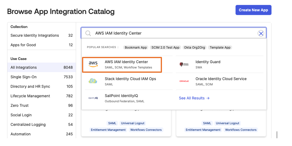
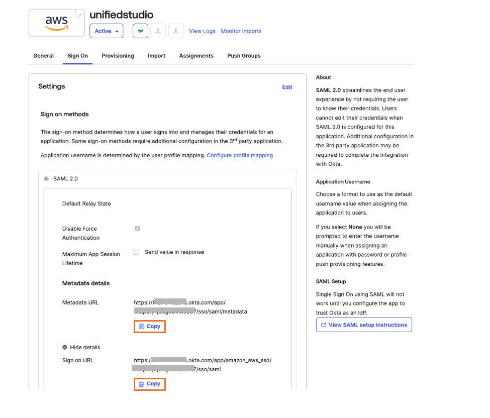
You are now ready to move to the AWS IAM Identity Center console to create an identity provider integration for your Okta instance.
Configure Okta as an identity provider in AWS IAM Identity Center
- Sign in to the AWS IAM Identity Center console as a user with administrative privileges
- In the left navigation menu, choose Settings and then, open the Identity source tab, choose Change Identity source from Actions dropdown as shown in Figure 5
 Figure 5: Selecting identity source in AWS IAM Identity Center
 - From Under Identity source, choose External Identity provider as shown in Figure 6

Figure 6: Choosing External Identity provider in AWS IAM Identity Center - You’ll need these configuration parameters for the next step. In Configure external identity provider section, under Service Provider metadata, do the following:
- Choose Download metadata file to download the AWS IAM Identity Center metadata file and save it on your system
- Copy these Service Provider metadata into a text file
- IAM Identity Center Assertion Consumer Service (ACS) URL
- IAM Identity Center issuer URL
- In Identity provider metadata section, under Idp SAML metadata, click on choose file and upload the metadata.xml file which you downloaded from okta in the previous step and then, choose Next as shown in Figure 7

Figure 7. Configuring okta as Identity Provider in AWS IAM Identity Center
- After you read the disclaimer and are ready to proceed, enter ACCEPT and then choose Change identity source to complete Okta as an Identity Provider in IAM Identity Center.
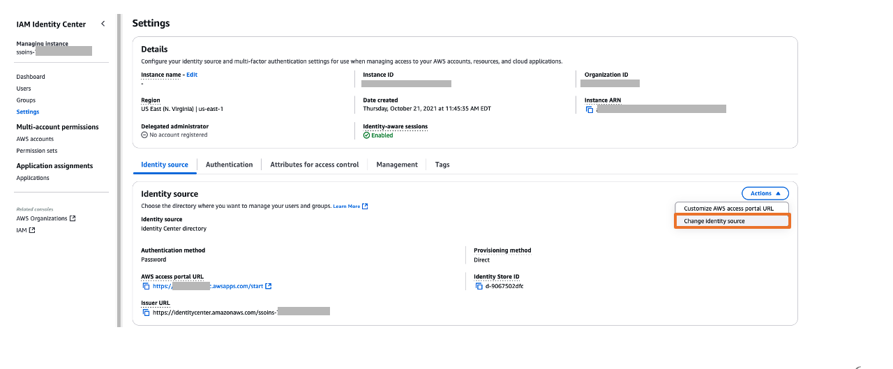 Figure 5: Selecting identity source in AWS IAM Identity Center
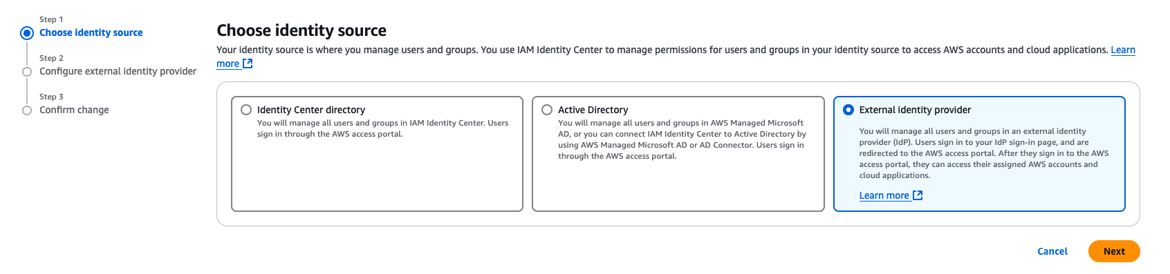
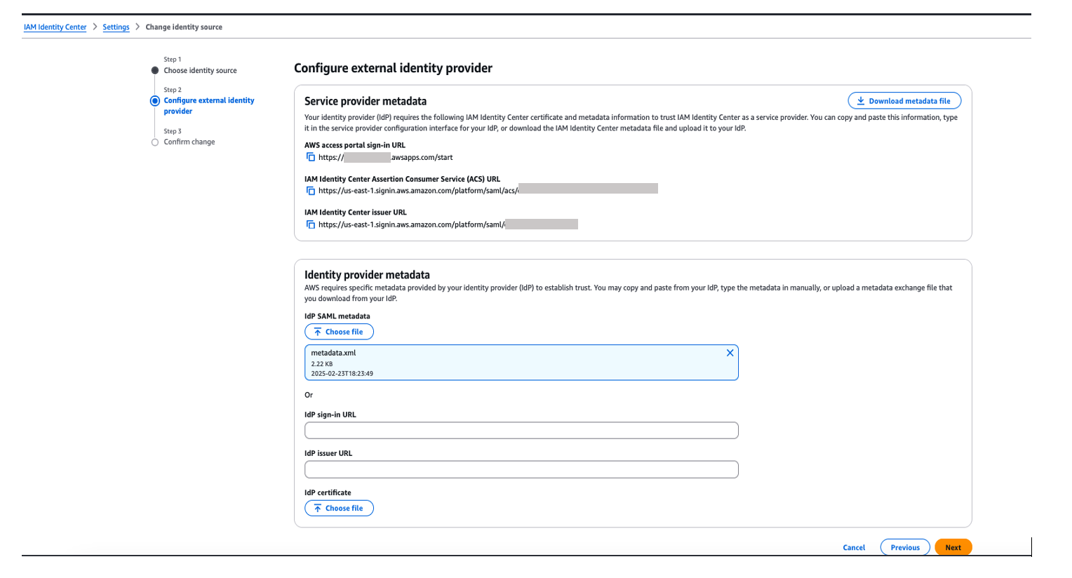
Connect AWS IAM Identity Center to Okta
- Sign into Okta and go to the admin console.
- In the left navigation pane, choose Applications, and then choose the Okta application called unifiedstudio which you created in the previous section
- In Sign On, choose Edit to complete SAML configuration. Under Advanced Sign-on Settings enter the following and then, choose Save to complete configuration as shown Figure 8.
- For the AWS SSO ACS URL, enter IAM Identity Center Assertion Consumer Service (ACS) URL
- For the AWS SSO issuer URL, enter IAM Identity Center issuer URL
- For the Application username format, choose Okta username from dropdown
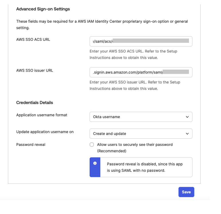 Figure 8. Configuring okta sign-on settings
Set up automatic provisioning of users and groups
In the AWS IAM Identity Center console, on the Settings page, locate the Automatic provisioning information box, and then choose Enable as shown in Figure 9. Copy these values to enable automatic provisioning.
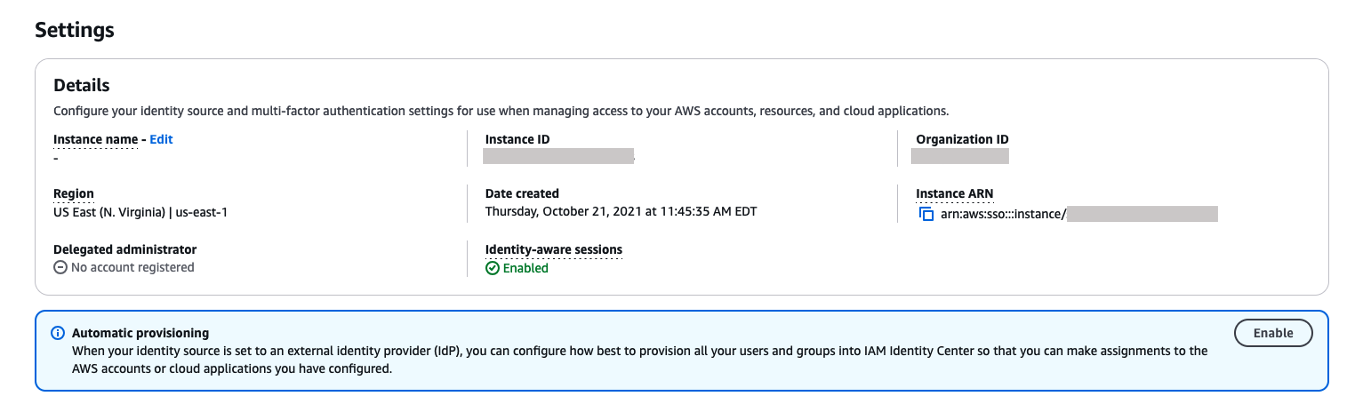
Figure 9. Enabling automatic provisioning in AWS IAM Identity Center
In the Inbound automatic provisioning dialog box, copy each of the values for the following options as shown in Figure 10 and then, choose Close
-
- SCIM endpoint
- Access token
You will use these values to configure provisioning in Okta in the next step.
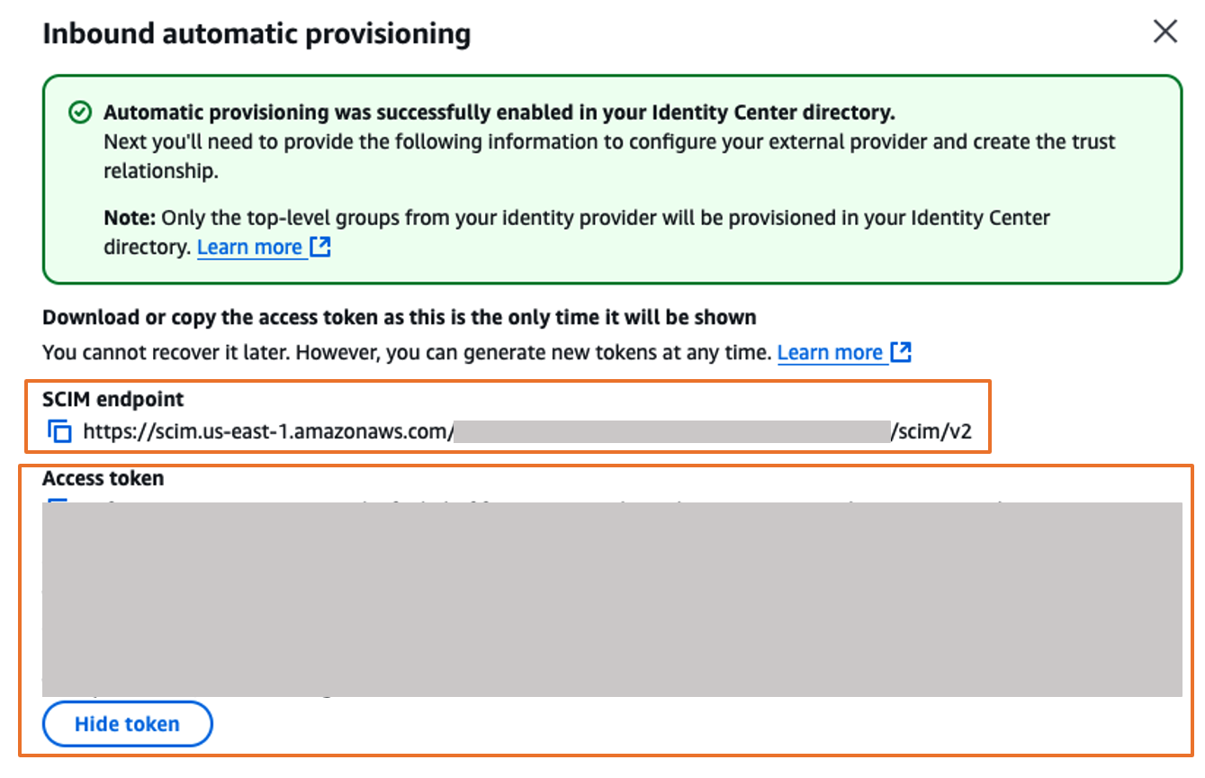 Figure 10. Automatic provisioning configuration parameters in AWS IAM Identity Center
Complete the Okta integration
- Sign into Okta and go to the admin console.
- In the left navigation pane, choose Applications, and then choose the Okta application called unifiedstudio which you created earlier.
- In Provisioning tab, choose Edit to complete auto provisioning between okta and AWS IAM Identity Center.
- Under Settings, choose Integration and then, choose Configure API integration and then, select Enable API integration to enable provisioning and enter the following using the SCIM provisioning values from AWS IAM Identity Center that you copied from the previous step as shown in Figure 11
For the Base URL, enter SCIM endpoint from IAM Identity Center
For the API Token, enter Access token from IAM Identity Center
For Import Groups, select Import groups option
And then, choose Test API Credentials to validate the SCIM provision and then, choose Save.

Figure 11: Automatic provisioning configuration in Okta
- Under Settings, choose Integration and then, choose Configure API integration and then, select Enable API integration to enable provisioning and enter the following using the SCIM provisioning values from AWS IAM Identity Center that you copied from the previous step as shown in Figure 11
- In the Provisioning tab, in the navigation pane under Settings, choose To App in the left navigation. Choose Edit, to Enable all options such as Create Users , Update User Attributes , Deactivate Users as shown in Figure 12 and then, choose Save.

Figure 12: Enabling Automatic provisioning configuration in Okta
- In the Assignments tab, choose Assign, and then Assign to Groups.
- Select the unifiedstudio group, choose Assign, and then, leave it to defaults on popup and then, choose Done to complete the Group assignment, as shown in Figure 13.
 Figure 13: Assigning unifiedstudio group to SAML application called unifiedstudio
 - In the Push Groups tab, under Push Groups drop-down list, select Find groups by name as shown in Figure 14.

Figure 14: Choosing okta groups to push them to AWS IAM Identity Center
- Select the unifiedstudio group, leave Push group memberships immediately default option and then, choose Save as shown in Figure 15.

Figure 15: Pushing okta groups to AWS IAM Identity Center
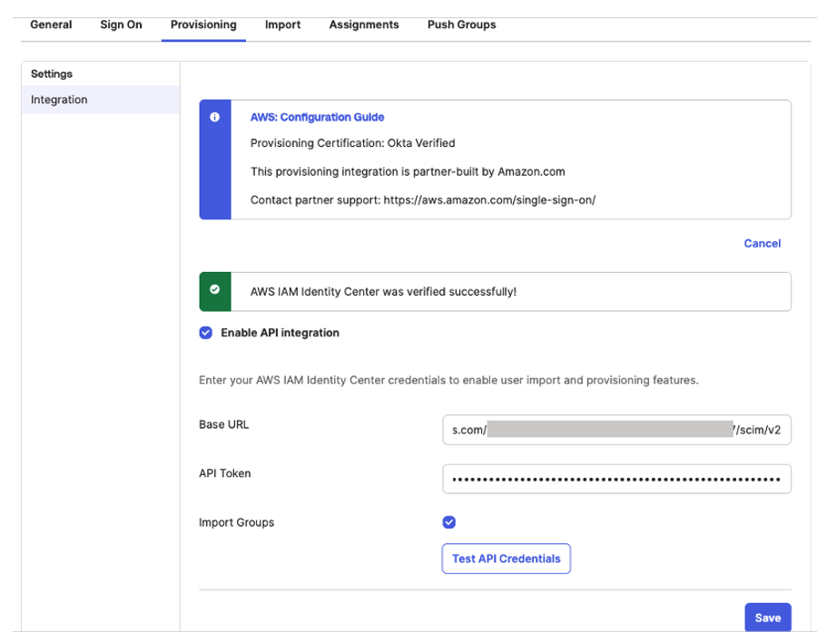
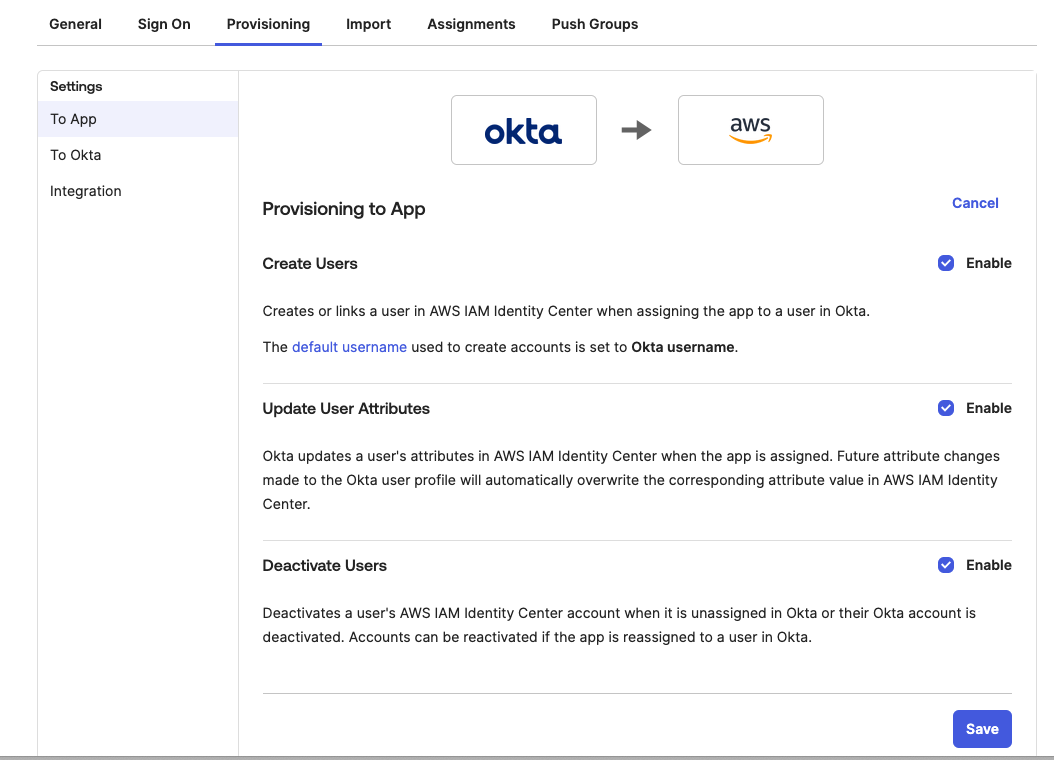
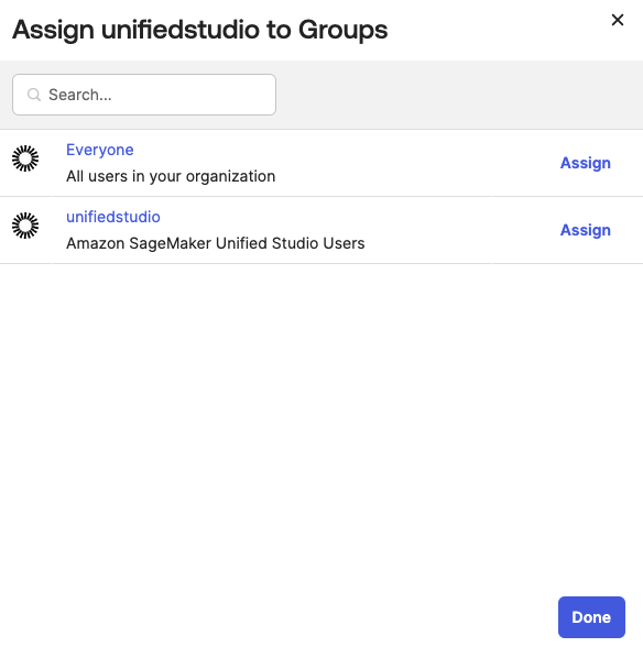 Figure 13: Assigning unifiedstudio group to SAML application called unifiedstudio
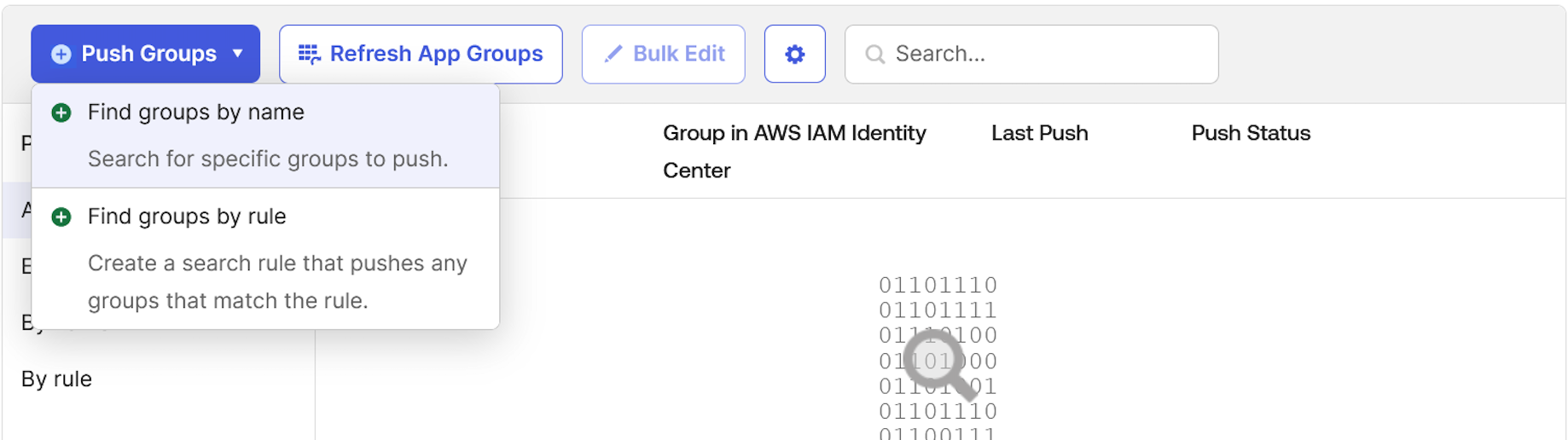
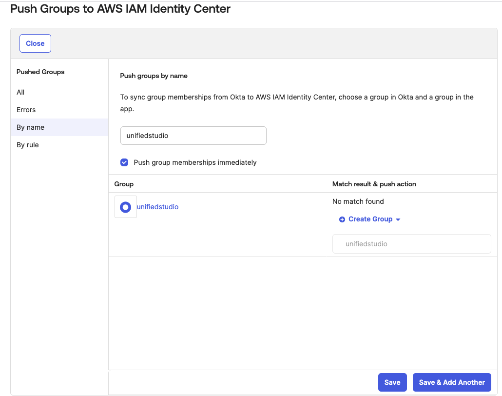
Return to AWS IAM Identity Center, and you should be able to see Okta group and Okta users in AWS IAM Identity Center groups and users as shown In Figure 16.
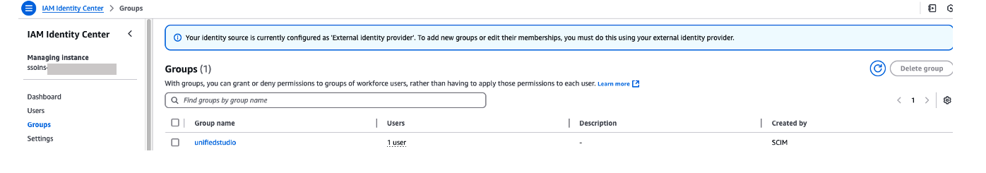
Figure 16: Okta user groups in AWS IAM Identity Center
Configure SageMaker Unified Studio for SSO
In this step, you will configure SSO user access to Amazon SageMaker Unified Studio for your Amazon SageMaker platform domain.
- Navigate to the Amazon SageMaker management console.
- In the left navigation menu, select Domains.
- Choose the Domain from the list for which you want to configure SAML user access.
- On the domain’s details page, choose Configure next to the Configure SSO user access.

Figure 17: Amazon SageMaker Unified Studio SSO configuration - On the Choose user authentication method page, choose IAM Identity Center. With IAM Identity Center, users configured through external Identity Providers (IdPs) get to access the domain’s Amazon SageMaker Unified Studio. Choose Next.

Figure 18: Choosing authentication - You can choose either Require assignments – which means you explicitly select users/groups that can access the domain or Do not require assignments – which allows all authorized Okta users and groups access to this domain.
- You have two options to configure how your users will access to Amazon SageMaker Unified studio with AWS IAM Identity Center federation with Okta
- Do not required Assignments – The access will be provided to Amazon SageMaker Unified Studio based on your Okta SAML application assignments either through Group assignments or Individual user assignments. For this example, when you choose Do not required assignments option, all the users within unifiedstudio Okta group will have access to Amazon SageMaker Unified Studio as we have assigned unifiedstudio Okta user group to unifiedstudio SAML application in Okta.
- Require Assignments – You need to add either Okta users or Okta group to Amazon SageMaker domain as shown in step 8. In step 8, you’ll add unifiedstudio Okta group into Amazon SageMaker domain so that all unifiedstudio Okta group users will get access to Amazon SageMaker Unified Studio. You can also provide an Individual Okta group users access to Amazon SageMaker unified studio through Amazon SageMaker domain console by adding SSO (okta user) user into the domain.
- Note that either an Individual user or group within Okta must be assigned to the AWS Identity center application (AWS IAM Identity Center from Okta application catalog. We renamed application label as unifiedstudio for this example) for both Do not require Assignments and Require Assignments options.

Figure 19. Amazon SageMaker Unified Studio SAML configuration
- You have two options to configure how your users will access to Amazon SageMaker Unified studio with AWS IAM Identity Center federation with Okta
- On the Review and save page, review your choices and then choose Save. Note that these settings are permanent once saved.

Figure 20. Review and confirm SAML configuration
- If you’ve chosen to require assignments, use the Add users and groups to add SAML users and groups to your domain.

Figure 21. Adding okta group into Amazon Sagemaker domain
- Now, users will be able to access the Amazon SageMaker Unified Studio using the Domain URL with their SSO credentials.
- You can explore different projects for your users and assign those projects based on your SAML user groups for fine-grained access controls. For example, you can create different SAML user groups based on their job function in Okta, assign those Okta groups to AWS IAM Identity Center app in Okta and then, assign those Okta SAML groups to respective project profiles in Amazon SageMaker Unified Studio. To perform project profiles assignments to respective groups, choose project profiles tab, click on respective project profiles like SQL analytics, choose Authorized users and groups tab and then, choose Add and pick SSO groups from drop down as shown in Figure 22. Finally choose Add users and groups to complete project profile assignment.

Figure 22. Assigning a project profile to okta group
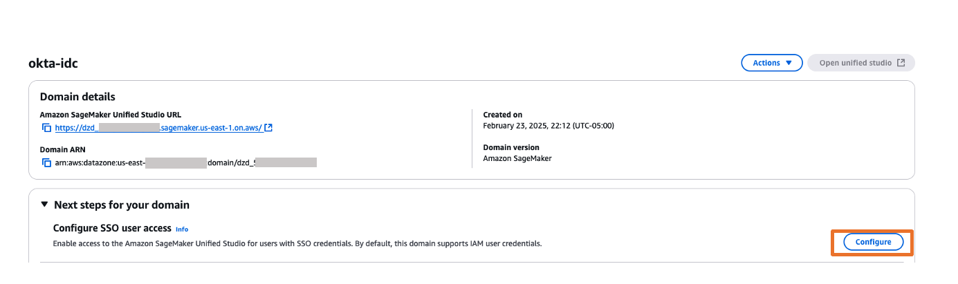
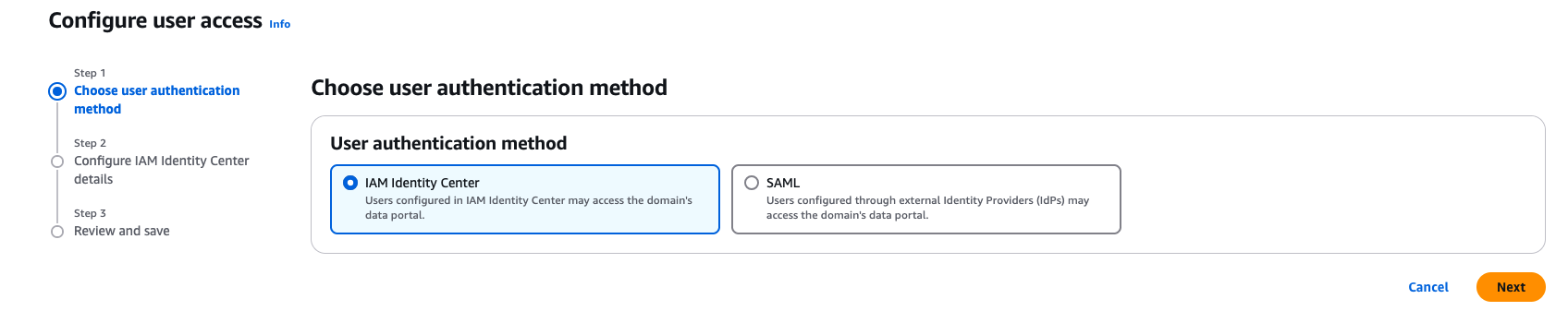
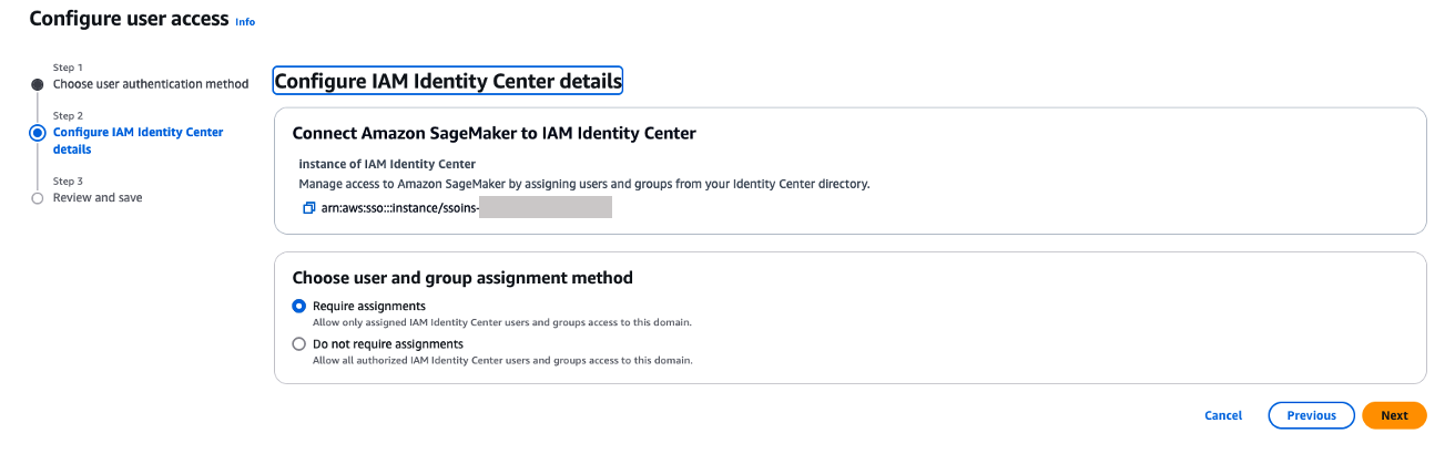
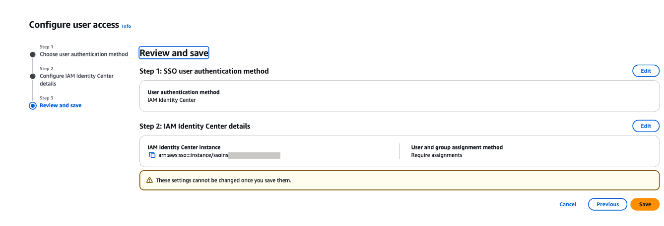
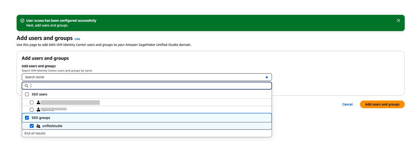
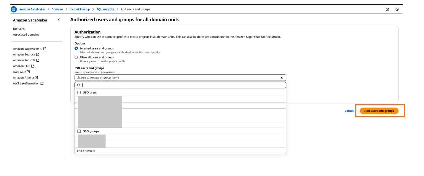
Test the setup
- The Amazon SageMaker Unified Studio URL can be found on the domain details page as shown in Figure 23. The first access to Amazon SageMaker Unified Studio URL redirects you to the Okta login screen.

Figure 23. Validating Okta user access with Amazon SageMaker Unified Studio
- Copy and paste the Amazon SageMaker Unified Studio URL in your browser and enter the user credentials.
- After successful login, you will be redirected to the Amazon SageMaker Unified Studio home page.


Figure 24. SAML authenticated Amazon SageMaker Unified Studio
- Once logged into Amazon SageMaker Unified Studio, you can assign authorization policies based on your requirements. Choose Govern and then choose, Domain units and choose your SageMaker domain to select suitable authorization policies. For this example, we are choosing project creation policy as shown in Figure 25.

Figure 25. Amazon SageMaker unified studio authorization policies - Choose Project membership policy and then choose ADD POLICY GRANT option to assign user groups or users to respective project. For this example, we are choosing project membership policy as shown in Figure 26.

Figure 26. Amazon SageMaker unified studio authorization policies assignment
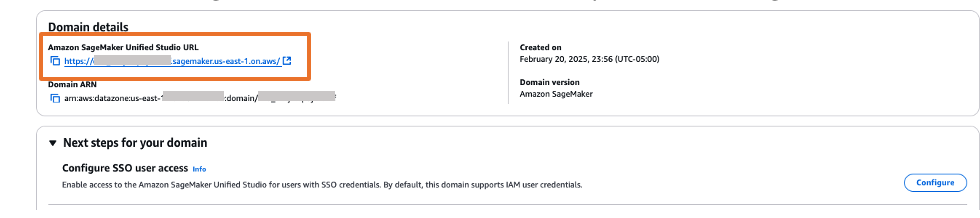
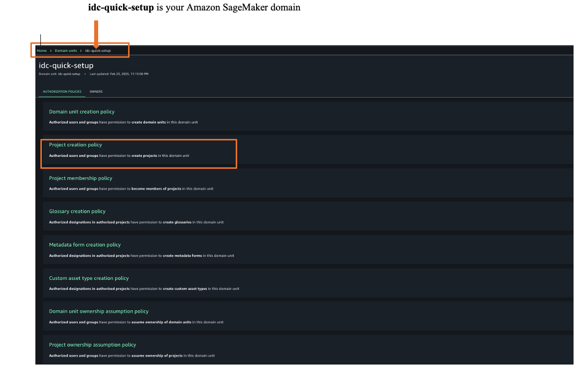
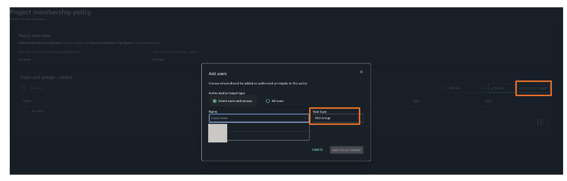
You’ve now successfully configured single sign-on for Amazon SageMaker Unified Studio using Okta credentials through AWS IAM Identity Center.
Clean up
To avoid ongoing charges, delete the resources you created:
- Deleting your Amazon SageMaker Unified Studio domain
- Deleting your Okta account (if needed)
Conclusion
In this post, we showed you how to set up Okta as an identity provider using SAML authentication for Amazon SageMaker Unified Studio access through AWS IAM Identity Center federation. This setup allows your users to access SageMaker Unified Studio with their existing corporate credentials, eliminating the need for separate AWS accounts.
Get started by checking the Amazon SageMaker Unified Studio Developer Guide, which provides guidance on how to build data and AI applications using Amazon SageMaker platform
About the authors
ORNL Discovery and Lux Powered by HPE and AMD Announced
Post Syndicated from Patrick Kennedy original https://www.servethehome.com/ornl-discovery-and-lux-powered-by-hpe-and-amd-announced/
ORNL announced the AMD-powered Discovery and Lux systems alongside HPE’s announcement of its new supercomputing portfolio
The post ORNL Discovery and Lux Powered by HPE and AMD Announced appeared first on ServeTheHome.
[$] BPF signing LSM hook change rejected
Post Syndicated from daroc original https://lwn.net/Articles/1042625/
BPF lets users load programs into a running kernel.
Even though BPF programs are checked by the verifier to
ensure that they stay inside certain limits, some users would still like to ensure
that only approved BPF programs are loaded. KP Singh’s
patches adding that capability to the kernel were accepted
in version 6.18, but not everyone is
satisfied with his implementation. Blaise Boscaccy, who has been working to get
a version of BPF code signing with better auditability
into the kernel for some time, posted
a patch set on top of Singh’s changes that alters the loading process to
not invoke security module hooks
until the entire loading process is complete.
The discussion on the patch
set is the continuation of a
long-running disagreement over
the interface for signed BPF programs.
Trump & Military Strikes #lastweektonight
Post Syndicated from LastWeekTonight original https://www.youtube.com/shorts/Mwc21oNdnaA