Today we turned off our Online Certificate Status Protocol (OCSP) service, as announced in December of last year. We stopped including OCSP URLs in our certificates more than 90 days ago, so all Let’s Encrypt certificates that contained OCSP URLs have now expired. Going forward, we will publish revocation information exclusively via Certificate Revocation Lists (CRLs).
We ended support for OCSP primarily because it represents a considerable risk to privacy on the Internet. When someone visits a website using a browser or other software that checks for certificate revocation via OCSP, the Certificate Authority (CA) operating the OCSP responder immediately becomes aware of which website is being visited from that visitor’s particular IP address. Even when a CA intentionally does not retain this information, as is the case with Let’s Encrypt, it could accidentally be retained or CAs could be legally compelled to collect it. CRLs do not have this issue.
We are also taking this step because keeping our CA infrastructure as simple as possible is critical for the continuity of compliance, reliability, and efficiency at Let’s Encrypt. For every year that we have existed, operating OCSP services has taken up considerable resources that can soon be better spent on other aspects of our operations. Now that we support CRLs, our OCSP service has become unnecessary.
At the height of our OCSP service’s traffic earlier this year, we handled approximately 340 billion OCSP requests per month. That’s more than 140,000 requests per second handled by our CDN, with 15,000 requests per second handled by our origin. We’d like to thank Akamai for generously donating CDN services for OCSP to Let’s Encrypt for the past ten years.
OpenAI has just announced their latest open-weight models — and we are excited to share that we are working with them as a Day 0 launch partner to make these models available in Cloudflare’s Workers AI. Cloudflare developers can now access OpenAI’s first open model, leveraging these powerful new capabilities on our platform. The new models are available starting today at @cf/openai/gpt-oss-120b and @cf/openai/gpt-oss-20b.
Workers AI has always been a champion for open models and we’re thrilled to bring OpenAI’s new open models to our platform today. Developers who want transparency, customizability, and deployment flexibility can rely on Workers AI as a place to deliver AI services. Enterprises that need the ability to run open models to ensure complete data security and privacy can also deploy with Workers AI. We are excited to join OpenAI in fulfilling their mission of making the benefits of AI broadly accessible to builders of any size.
The technical model specs
The OpenAI models have been released in two sizes: a 120 billion parameter model and a 20 billion parameter model. Both of them are Mixture-of-Experts models – a popular architecture for recent model releases – that allow relevant experts to be called for a query instead of running through all the parameters of the model. Interestingly, these models run natively at an FP4 quantization, which means that they have a smaller GPU memory footprint than a 120 billion parameter model at FP16. Given the quantization and the MoE architecture, the new models are able to run faster and more efficiently than more traditional dense models of that size.
These models are text-only; however, they have reasoning capabilities, tool calling, and two new exciting features with Code Interpreter and Web Search (support coming soon). We’ve implemented Code Interpreter on top of Cloudflare Containers in a novel way that allows for stateful code execution (read on below).
The model on Workers AI
We’re landing these new models with a few tweaks: supporting the new Responses API format as well as the historical Chat Completions API format (coming soon). The Responses API format is recommended by OpenAI to interact with their models, and we’re excited to support that on Workers AI.
If you call the model through:
Workers Binding, it will accept/return Responses API – env.AI.run(“@cf/openai/gpt-oss-120b”)
REST API on /run endpoint, it will accept/return Responses API – https://api.cloudflare.com/client/v4/accounts/<account_id>/ai/run/@cf/openai/gpt-oss-120b
REST API on new /responses endpoint, it will accept/return Responses API – https://api.cloudflare.com/client/v4/accounts/<account_id>/ai/v1/responses
REST API for OpenAI Compatible endpoint, it will return Chat Completions (coming soon)– https://api.cloudflare.com/client/v4/accounts/<account_id>/ai/v1/chat/completions
Code Interpreter + Cloudflare Sandboxes = the perfect fit
To effectively answer user queries, Large Language Models (LLMs) often struggle with logical tasks such as mathematics or coding. Instead of attempting to reason through these problems, LLMs typically utilize a tool call to execute AI-generated code that solves these problems. OpenAI’s new models are specifically trained for stateful Python code execution and include a built-in feature called Code Interpreter, designed to address this challenge.
We’re particularly excited about this. Cloudflare not only has an inference platform (Workers AI), but we also have an ecosystem of compute and storage products that allow people to build full applications on top of our Developer Platform. This means that we are uniquely suited to support the model’s Code Interpreter capabilities, not only for one-time code execution, but for stateful code execution as well.
We’ve built support for Code Interpreter on top of Cloudflare’s Sandbox product that allows for a secure environment to run AI-generated code. The Sandbox SDK is built on our latest Containers product and Code Interpreter is the perfect use case to bring all these products together. When you use Code Interpreter, we spin up a Sandbox container scoped to your session that stays alive for 20 minutes, so the code can be edited for subsequent queries to the model. We’ve also pre-warmed Sandboxes for Code Interpreter to ensure the fastest start up times.
We’ll be publishing an example of how you can use the gpt-oss model on Workers AI and Sandboxes with the OpenAI SDK to make calls to Code Interpreter on our Developer Docs.
Give it a try!
We’re beyond excited for OpenAI’s new open models, and we hope you are too. Super grateful to our friends from vLLM and HuggingFace for supporting efficient model serving on launch day. Read up on the Developer Docs to learn more about the details and how to get started on building with these new models and capabilities.
Proxmox Virtual Environment 9.0, based on Debian 13
(“trixie”), has been released. Notable
new features include snapshots for thick-provisioned LVM shared
storage, affinity rules for high availability (HA) clusters, and a
modernized mobile web interface for managing Proxmox systems. See the release
notes and known
issues for more details about the release.
In today’s digital landscape, efficient email management is crucial for businesses of all sizes. Amazon Simple Email Service (Amazon SES) has long been a go-to solution for handling transactional and marketing emails. Through Mail Manager, Amazon SES offers powerful tools to enhance your email infrastructure, particularly for outbound email handling and archiving.
In this post, we explore how Mail Manager can modernize your approach to outbound email management. We’ll dive into the various options available for controlling email flows and archiving all outgoing emails. By the end of this article, you’ll have a clear understanding of how you can use Mail Manager to:
Strengthen your email infrastructure
Simplify outbound email workflow management
Help meet compliance through robust email archiving
In this post, we consider a real-world customer use case from a university where students should receive clean emails free from malware and phishing attempts. Amazon SES Mail Manager provides a comprehensive email pipeline that handles security screening, message archival, and reliable delivery. By implementing this system, the university significantly improved its email infrastructure, helping to ensure that important communications reach students safely and efficiently.
Walkthrough
In this walkthrough, we guide you through the process of configuring Amazon SES Mail Manager with the following components:
Traffic policy: You’ll create a traffic policy designed to help ensure that students receive only clean, secure emails. The default action is set to Deny all, providing a strict baseline. The policy includes two key statements connected by an OR condition. Policy Statement 1 allows emails if the recipient address is in the Valid-Address list. Policy Statement 2 allows emails that meet all of the following conditions: not listed in Abusix Guardian Mail, recipient address is not in the Invalid-Email-List, and uses TLS protocol version 1.3 or higher. This configuration effectively filters potential threats while allowing legitimate communications to reach students’ inboxes, maintaining a secure email environment for the university.
Rule set: You’ll create a rule set containing two rules that execute in sequential order:
Rule 1: Scan and isolate malicious content: Scans messages and, if the scan fails, stores emails in an Amazon Simple Storage Service (Amazon S3) bucket for further validation and halts sending email.
Rule 2: Archive and send clean emails to recipients: Archives all outgoing emails for audit and compliance after passing the security scan and routes emails to recipients.
Ingress endpoint: You’ll create a Mail Manager ingress endpoint that will receive, route, and manage emails based on your configured policies and rules.
After setting up these components, you’ll use sample Python code to send an email through the ingress endpoint. To verify functionality, we’ll check the email archive to confirm that all incoming emails are archived for compliance or audit purposes and confirm email is received in the intended inbox. The workflow is shown in the following figure.
Prerequisites
Before beginning, make sure that you have completed domain verification in your desired AWS Region and moved out of the Amazon SES sandbox. Domain verification is a crucial first step that validates your authority to send emails through SES from your domain. In this tutorial, you’ll use a sample Python program to send emails programmatically through an ingress SMTP endpoint. You can run this program either on your local machine or using AWS CloudShell.
A user signed in to the AWS Management Console must have permissions to the preceding above services.
Before creating traffic policies and rule sets, you will first set up Email Add Ons, and email archiving, and AWS Identity and Access Management (IAM) roles, which will be needed while creating traffic policies and rules.
Step 1: Enable Email Add Ons for Amazon SES Mail Manager
To implement security features such as malicious content scanning in your email workflow, first enable the necessary Email Add Ons:
Open the AWS Management Console for Amazon SES.
Choose Mail Manager and then Email Add Ons.
Select your desired Add Ons:
Trend Micro Virus Scanning
Abusix Guardian Mail
Spamhaus Domain Block List (DBL)
Vade Advanced Email Security
Choose Enable.
Important Notes:
Email Add Ons are third-party security products integrated with Mail Manager
Once subscribed, you can use them in your traffic policies or rule sets
As part of this post, you will be using the Abusix Guardian Mail and Vade Advanced Email Security Add Ons to enhance email security posture. It doesn’t mean you have to use all of them—you can subscribe to the ones that best fit your requirements based on your use case.
Step 2: Configure an email archive for compliance and retention
You will create an email archive to store outgoing messages to use as part of configuring Rule 2. This archive will serve as a repository for outgoing messages.
Navigate to Mail Manager and then to Email Archiving.
Choose Create archive.
Complete the archive configuration:
Enter a unique name in the Archive name field.
(Optional) Select a retention period to override the default of 180 days.
(Optional) Set up encryption by either entering your own AWS Key Management System (AWS KMS) key in the KMS key ARN field or selecting Create new key.
Choose Create archive.
After being created, this archive will store your emails according to the rules you’ll define in the next step.
Step 3: Create and S3 bucket and IAM role for S3 access
When emails fail the Vade security scan, they need to be stored securely for further investigation. In this step, we’ll create an S3 bucket to store these flagged emails and set up the necessary IAM permissions.
Create an S3 bucket to quarantine suspicious and malicious emails identified by the Vade scanner. This bucket will store these emails for further investigation by the security team. Note the bucket name, because you’ll need it in the next step.
Create an IAM role that allows Mail Manager to upload suspicious emails to an S3 bucket. This IAM role will be used in Rule 1 when configuring the Write to S3 rule action for storing emails that fail the security scan.
Go to the IAM console.
Choose Roles and then choose Create role.
For trusted entity, select Custom trust policy and paste the following (replace "XXXXXXXXXXX" with your AWS account ID).
Step 4: Create and IAM role permission policy for send to internet rule action
Configure an IAM role that permits Mail Manager to send emails to external domains. This role will be referenced in Rule 2 for delivering validated emails to recipients.
You can either:
Use the same IAM role created in Step 3 and add this policy, or
Create a new IAM role and add the following permission policy (Replace example.com with your verified domain, "XXXXXXXXXXX" with your AWS account ID and my-configuration-set with your configuration set name if applicable).
This policy grants the necessary permissions to send emails to recipients on the internet, which will be used in rule 2 of your rule set.
Choose Add permissions and then select Create inline policy.
Paste the preceding JSON and choose Review policy.
Enter a name for the policy and choose Create policy.
If you create a new role, name it appropriately and choose Create role.
Step 5: Create a traffic policy
Traffic policies serve as security checkpoints for your email infrastructure, controlling which messages can enter your system based on defined security rules. To create a traffic policy that enforces security requirements for your emails:
Open the Amazon SES console.
Go to Mail Manager and choose Traffic policies.
Choose Create traffic policy.
Enter a unique name for your policy.
Set Default action to Allow (this handles emails that don’t match any specific rules).
Add policy statements by choosing Add new policy statement:
Choose Deny for emails that don’t meet security requirements.
Add condition: TLS Protocol Version select Less than and then select 1.2.
Add conditions for any Email Add-Ons you’ve subscribed to, such as Spamhaus, Abusix, and so on.)
Choose Create traffic policy.
Traffic policies are evaluated in a specific sequence:
First, all Deny policy statements are evaluated in order. If any match, the email is immediately blocked and no further evaluation occurs.
If no Deny statements match, all Allow policy statements are evaluated in order. Multiple statements within a policy are connected by OR logic. If any statement matches, the email is allowed.
Within each individual policy statement, multiple conditions are connected by AND logic. All conditions must be true for the statement to match.
If no policy statements match (neither Deny nor Allow), the default action of the traffic policy (either Allow or Deny) is applied.
In this step, you’ll establish a robust policy that enforces strict TLS security protocols while harnessing the power of specialized email security add-ons such as Abusix Guardian Mail to preemptively identify and block potentially harmful messages before they can penetrate your system. In this traffic policy configuration, you’ll create two policy statements that work together to provide security and flexibility:
Default policy statement:
Deny-by-default where all email traffic is initially blocked unless explicitly allowed by below policy statements
Policy statement 1:
Allows emails if the recipient address is in a list called Valid-Address
Policy statement 2 (with three conditions connected by AND):
Must NOT be listed in Abusix Guardian Mail (FALSE condition)
The recipient address must NOT be in the Invalid-Email-List
The TLS protocol version must be at least TLS 1.3
In basic terms, this policy will allow emails that either:
Have recipients from an approved address list, or
Meet all three security conditions (not deny-listed, not on the invalid list, and using secure TLS 1.3)
Step 6: Create a rule set
Rule sets define how your emails are processed after they pass through your traffic policy. In this example, the rule set establishes a sequential email processing workflow. First, you will perform email scanning (marking and segregating spam emails while allowing clean ones to proceed) and archiving outgoing messages, then finally delivering clean messages to recipients. To create a rule set:
Open the Amazon SES console.
Go to Mail Manager and choose Rule sets.
Choose Create rule set.
Enter a unique name for your rule set.
On the rule set’s overview page, choose Edit, then choose Create new rule
Step 7: Create rules
After creating your rule set, you’ll need to add rules that define how your emails are processed. Follow these steps to create and configure your rules:
On the rule set’s overview page, choose Edit, then Create new rule.
In the Rule details sidebar, enter a unique name for your rule.
Add conditions or exceptions as needed:
Select Add new condition to specify what messages the rule applies to.
Select EXCEPT in the case of and select Add new exception for exclusions.
Configure actions by choosing Add new action.
For multiple actions, use the up and down arrows to set the execution order.
When finished creating your rules, choose Save rule set to apply your changes.
Rule 1: Scan and isolate malicious content
This rule targets emails flagged by Vade Advanced Email Security as potentially harmful. It applies to messages identified as scams, suspect content, phishing attempts, or containing malware. When a message is flagged as malicious, the rule marks it with a custom header, stores a copy in Amazon S3 for investigation, and prevents it from reaching recipients. An exception allows emails with Action required in the subject line to bypass this security check.
Use the following settings to create and configure Rule 1:
Value: Select scam, suspect, phishing, and malware.
Actions:
Add header: For Key, enter X-vedacheck and for Value, enter failed.
Write to S3: Enter the name of an S3 bucket to store the message for investigation.
Drop: Stop processing the message.
Rule 2: Archive and send clean emails to recipients
This final rule processes messages that have successfully passed through the previous security checks. With no additional conditions, it forwards clean emails to their intended recipients, completing the secure email delivery workflow for the university’s communication system. Use the following settings to create and configure Rule 2:
Rule name: SendEmail
Action:
Add header: For Key , enter Add X-vedacheck with a Value of Approved.
Archive resource name: Select your Mail Manager archive (Email_Archive)
Send to internet: Send email to intended recipient.
The workflow makes sure that:
All outbound emails are securely archived
Each email undergoes scanning
Scan results are documented in email headers
Clean emails are delivered to their intended recipients
Step 8 : Store password in AWS Secrets Manager for the ingress endpoint
Before creating an ingress endpoint, you need to set up a password in AWS Secrets Manager:
Go to the AWS Secrets Manager console and choose Store a new secret.
Select Other type of secret.
Enter password as the key and your desired password as the value.
For Encryption key: Use a custom KMS key (not AWS managed keys).
KMS customer managed key (CMK) key policy for ingress endpoint. Replace XXXXXXXXXXX with your AWS account ID.
You’ll need these details when configuring your email client or application to send emails through this endpoint.
Step 10: Send email using an ingress endpoint
The following Python sample code can be executed from your local machine with the appropriate AWS credentials, but for this post you’ll run the script from the AWS CloudShell terminal from within the Amazon SES console. When running the sample Python code, the email will pass through an ingress endpoint and, if all policies are met, the email will be sent to the recipient’s email address.
INGRESS_USERNAME = inp-XXXXXXXXXXXX is your ingress endpoint username.
Recipient and sender= [email protected] is your verified sender and recipient email addresses.
Save the file.
Run the script:
python3 send_email.py
Verify the results:
Check the recipient’s inbox for the email.
Check the Mail Manager archive to confirm the message was archived.
To search the Mail Manager archive for the specific message sent by the Python script:
Navigate to the Amazon SES console and choose Mail Manager.
Under Email Archiving, choose the Search archive tab.
Under Archive, select the archive you created and choose Search. This should return all the emails you have sent.
Clean up
Clean up your AWS environment by removing all resources created during this walkthrough, including Mail Manager configurations, S3 buckets, secrets, and any associated Lambda functions.
Conclusion
In this post, we’ve demonstrated the implementation of sophisticated traffic policies, multi-layered rule systems, and automated archiving capabilities—all seamlessly integrated into a scalable architecture. The ability of Amazon SES Mail Manager to enforce TLS requirements, conduct email scanning, and maintain searchable archives while providing programmatic access through ingress endpoints makes it an invaluable tool for organizations seeking to modernize their email infrastructure.As businesses continue to rely heavily on email communication, Amazon SES Mail Manager emerges as a powerful ally, helping organizations navigate the complexities of modern digital correspondence while ensuring rock-solid security, seamless compliance, and optimal efficiency.
Many organizations running VMware workloads on premises want to move to the cloud to benefit from improved scalability, reliability, and access to cloud services, but migrating these workloads often requires substantial changes to applications and infrastructure configurations. Amazon EVS lets customers continue using their existing VMware expertise and tools without having to re-architect applications or change established practices, thereby simplifying the migration process while providing access to AWS’s scale, reliability, and broad set of services.
With Amazon EVS, you can run VMware workloads directly in your Amazon VPC. This gives you full control over your environments while being on AWS infrastructure. You can extend your on-premises networks and migrate workloads without changing IP addresses or operational runbooks, reducing complexity and risk.
Key capabilities and features
Amazon EVS delivers a comprehensive set of capabilities designed to streamline your VMware workload migration and management experience. The service enables seamless workload migration without the need for replatforming or changing hypervisors, which means you can maintain your existing infrastructure investments while moving to AWS. Through an intuitive, guided workflow on the AWS Management Console, you can efficiently provision and configure your EVS environments, significantly reducing the complexity to migrate your workloads to AWS.
With Amazon EVS, you can deploy a fully functional VCF environment running on AWS in a few hours. This process eliminates many of the manual steps and potential configuration errors that often occur during traditional deployments. Furthermore, with Amazon EVS you can optimize your virtualization stack on AWS. Given the VCF environment runs inside your VPC, you have full full administrative access to the environment and the associated management appliances. You also have the ability to integrate third-party solutions, from external storage such as Amazon FSx for NetApp ONTAP or Pure Cloud Block Store or backup solutions such as Veeam Backup and Replication.
The service also gives you the ability to self-manage or work with AWS Partners to build, manage, and operate your environments. This provides you with flexibility to match your approach with your overall goals.
Setting up a new VCF environment
Organizations can streamline their setup process by ensuring they have all the necessary pre-requisites in place ahead of creating a new VCF environment. These prerequisites include having an active AWS account, configuring the appropriate AWS Identity and Access Management (IAM) permissions, and setting up a Amazon VPC with sufficient CIDR space and two Route Server endpoints, with each endpoint having its own peer. Additionally, customers will need to have their VMware Cloud Foundation license keys ready, secure Amazon EC2 capacity reservations specifically for i4i.metal instances, and prepare their VLAN subnet information planning.
To help ensure a smooth deployment process, we’ve provided a Getting started hub, which you can access from the EVS homepage as well as a comprehensive guide in our documentation. By following these preparation steps, you can avoid potential setup delays and ensure a successful environment creation.
Let’s walk through the process of setting up a new VCF environment using Amazon EVS.
You will need to provide your Site ID, which is allocated by Broadcom when purchasing VCF licenses, along with your license keys. To ensure a successful initial deployment, you should verify you have sufficient licensing coverage for a minimum of 256 cores. This translates to at least four i4i.metal instances, with each instance providing 64 physical cores.
This licensing requirement helps you maintain optimal performance and ensures your environment meets the necessary infrastructure specifications. By confirming these requirements upfront, you can avoid potential deployment delays and ensure a smooth setup process.
Once you have provided all the required details, you will be prompted to specify your host details. These are the underlying Amazon EC2 instances that your VCF environment will get deployed in.
Once you have filled out details for each of your host instances, you will need to configure your networking and management appliance DNS details. For further information on how to create a new VCF environment on Amazon EVS, follow the documentation here.
After you have created your VCF environment, you will be able to look over all of the host and configuration details through the AWS Console.
Additional things to know
Amazon EVS currently supports VCF version 5.2.1 and runs on i4i.metal instances. Future releases will expand VCF versions, licensing options, and more instance type support to provide even more flexibility for your deployments.
Amazon EVS provides flexible storage options. Your Amazon EVS local Instance storage is powered by VMware’s vSAN solution, which pools local disks across multiple ESXi hosts into a single distributed datastore. To scale your storage, you can leverage external Network File System (NFS) or iSCSI-based storage solutions. For example, Amazon FSx for NetApp ONTAP is particularly well-suited for use as an NFS datastore or shared block storage over iSCSI.
Additionally, Amazon EVS makes connecting your on-premises environments to AWS simple. You can connect from on-premises vSphere environment into Amazon EVS using a Direct Connect connection or a VPN that terminates into a transit gateway. Amazon EVS also manages the underlying connectivity from your VLAN subnets into your VMs.
AWS provides comprehensive support for all AWS services deployed by Amazon EVS, handling direct customer support while engaging with Broadcom for advanced support needs. Customers must maintain AWS Business Support on accounts running the service.
Availability and pricing
Amazon EVS is now generally available in US East (N. Virginia), US East (Ohio), US West (Oregon), Europe (Frankfurt), Europe (Ireland), and Asia Pacific (Tokyo) AWS Regions, with additional Regions coming soon. Pricing is based on the Amazon EC2 instances and AWS resources you use, with no minimum fees or upfront commitments.
Effective log analysis is essential for maintaining the health and performance of modern applications. Amazon OpenSearch Service stands out as a powerful, fully managed solution for log analytics and observability. With its advanced indexing, full-text search, and real-time analytics capabilities, OpenSearch Service makes it possible for organizations to seamlessly ingest, process, and search log data across diverse sources—including AWS services like Amazon CloudWatch, VPC Flow Logs, and more.
With OpenSearch Dashboards, you can turn indexed log data into actionable visualizations that reveal insights and help detect anomalies. By querying data stored in OpenSearch Service, you can extract relevant information and display it using a variety of visualization types—such as line charts, bar graphs, pie charts, heatmaps, and more. These tools make it effortless to monitor system behavior, spot trends, and quickly identify issues in your environment.
This post demonstrates how to harness OpenSearch Dashboards to analyze logs visually and interactively. With this solution, IT administrators, developers, and DevOps engineers can create custom dashboards to monitor system behavior, detect anomalies early, and troubleshoot issues faster through interactive charts and graphs.
Solution overview
In this post, we show how to create an index pattern in OpenSearch Dashboards, create two types of visualizations, and display these visualizations on a custom dashboard. We also demonstrate how to export and import visualizations.
Prerequisites
Before diving into log analysis with OpenSearch Dashboards, you must have the following:
For this post, we work with the following log sources, which have already been ingested into an OpenSearch Service cluster as part of the prerequisite steps:
Complete the following steps to access OpenSearch Dashboards:
On the OpenSearch Service console, choose Domains in the navigation pane.
Check if your domain status shows as Active.
Choose your domain to open the domain details page.
Choose the OpenSearch Dashboards URL to open it in a new browser window.
Authenticate into OpenSearch Dashboards using one of the supported methods.
Create an index pattern
After you’re logged in to OpenSearch Dashboards, you must create an index pattern. An index pattern allows OpenSearch Dashboards to locate indexes to search. Complete the following steps
In OpenSearch Dashboards, expand the navigation pane and choose Dashboard Management under Management.
Choose Index patterns in the navigation pane.
Choose Create index pattern.
For Index pattern name, enter a name (for example, log-aws-cloudtrail-*).
Choose Next step.
For Time field¸ choose @timestamp.
Choose Create index pattern.
Create visualizations
Now that the index pattern is created, let’s create some visualizations. For this post, we create a pie chart and an area graph.
Create a pie chart
Complete the following steps to create a pie chart:
In OpenSearch Dashboards, choose Visualize in the navigation pane.
Choose Create visualization.
Choose Pie as the visualization type.
For Source¸ choose log-aws-cloudtrail-*.
Under Buckets¸ choose Add and Split slices.
For Aggregation, choose Terms.
For Field, choose eventName.
For Size, enter 10.
Leave all other parameters as default and choose Update.
Please refer Export and import visualizations for how to import the samples.
Create a dashboard
Now we will combine the visualizations we just created into a dashboard. A dashboard serves as a customizable interface that consolidates multiple visualizations, saved searches, and various content into a comprehensive view of data. Users can combine diverse visual elements—including charts, graphs, metrics, and tables—into a single cohesive display that can be arranged and resized on a flexible grid layout. You can simultaneously apply filters and time ranges across multiple visualizations, creating a coordinated analytical experience. Complete the following steps to create a dashboard:
In OpenSearch Dashboards, choose Dashboards in the navigation pane.
Choose Create new dashboard.
Choose Add on the menu bar.
Search for and choose the visualizations you created.
You can resize panels by dragging their corners to adjust dimensions. To modify the layout arrangement, you can drag the top portion of panels, which allows you to organize them horizontally in a row formation. When working with tabular visualizations, the system provides a convenient option to export your results in CSV format for further analysis or reporting purposes.
Please refer Export and import visualizations for how to import the samples.
The following screenshot shows the CloudTrail dashboard displaying both visualizations.
Export and import visualizations
In OpenSearch, an NDJSON file is used to import and export saved objects, such as dashboards, visualizations, maps, and index template. The NDJSON file provides a streamlined approach for handling large datasets by representing each JSON object on a separate line. This format enables efficient import/export operations, simplified data migration between environments, and seamless sharing of complex dashboard configurations. Organizations can back up and restore critical visualizations, saved searches, and dashboard settings while maintaining their integrity. The format’s structure reduces memory overhead during large transfers and improves processing speed for bulk operations. NDJSON’s human-readable nature also facilitates troubleshooting and manual editing when necessary, making it an invaluable tool for maintaining OpenSearch Dashboards deployments across development, testing, and production environments.
Export a visualization
Complete the following steps to export a visualization:
In OpenSearch Dashboards, choose Saved objects in the navigation pane.
Search for and select your object (in this case, a visualization), then choose Export.
The NDJSON file is downloaded in your local host.
Import a visualization
Complete the following steps to import a visualization:
In OpenSearch Dashboards, choose Saved objects in the navigation pane.
Choose Import.
Choose the first NDJSON file to be imported from your local host.
Select Create new objects with random IDs.
Choose Import.
Choose Done.
Choose Import.
You can now open the imported object.
The following screenshot shows our updated dashboard.
Clean up
To clean up your resources, delete the OpenSearch Service domain and relevant information stored or visualizations created on the domain. You will not be able to recover the data after you delete it.
On the OpenSearch Service console, choose Domains in the navigation pane.
Select the domain you created and choose Delete.
Conclusion
OpenSearch Dashboards is a powerful tool for transforming raw log data into actionable visualizations that drive insights and decision-making. In this post, we’ve shown how to create visualizations like pie charts and area graphs, build comprehensive dashboards, and efficiently export and import your work using NDJSON files. By using the fully managed OpenSearch Service features, organizations can focus on extracting valuable insights rather than managing infrastructure, ultimately enhancing their observability posture and operational efficiency.
To further enhance your OpenSearch proficiency, consider exploring advanced visualization options such as heat maps, gauge charts, and geographic maps that can represent your data in more specialized ways. Implementing automated alerting based on predefined thresholds will help you proactively identify anomalies before they become critical issues. You can also use OpenSearch’s powerful machine learning capabilities for sophisticated anomaly detection and predictive analytics to gain deeper insights from your log data. As your implementation grows, customizing security settings with fine-grained access controls will provide appropriate data visibility across different teams in your organization.
Smita Singh is a Senior Solutions Architect at AWS. She focuses on defining technical strategic vision and works on architecture, design, and implementation of modern, scalable platforms for large-scale global enterprises and SaaS providers. She is a data, analytics, and generative AI enthusiast and is passionate about building innovative, highly scalable, resilient, fault-tolerant, self-healing, multi-tenant platform solutions and accelerators.
Dipayan Sarkar is a Specialist Solutions Architect for Analytics at AWS, where he helps customers modernize their data platform using AWS analytics services. He works with customers to design and build analytics solutions, enabling businesses to make data-driven decisions.
Healthcare systems face significant challenges managing vast amounts of data while maintaining regulatory compliance, security, and performance. This post explores strategies for implementing a multi-tenant healthcare system using Amazon OpenSearch Service.
In this context, tenants are distinct healthcare entities, sharing a common platform while maintaining isolated data environments. Hospital departments (like emergency, radiology, or patient care), clinics, insurance providers, laboratories, and research institutions are examples of these tenants.
In this post, we address common multi-tenancy challenges and provide actionable solutions for security, tenant isolation, workload management, and cost optimization across diverse healthcare tenants.
Understanding multi-tenant healthcare systems
Tenants in healthcare systems are diverse and have distinct requirements. For example, emergency departments need round-the-clock high availability with subsecond response times for patient care, along with strict access controls for sensitive trauma data. Research departments run complex, resource-intensive queries that are less time-sensitive but require robust anonymization protocols to maintain HIPAA compliance when working with patient data. Outpatient clinics operate during business hours with predictable usage patterns and moderate performance requirements. Administrative systems focus on financial data with scheduled batch processing and require access to billing information and insurance details only. Specialty departments like radiology and cardiology have unique requirements specific to the tasks they perform. For example, radiology requires high storage capacity and bandwidth for large medical imaging files, along with specialized indexing for metadata searches.
Understanding tenant requirements is essential for designing an effective multi-tenant architecture that balances resource sharing with appropriate isolation while maintaining regulatory compliance.
Isolation models
OpenSearch’s hierarchical structure consists of four main levels. At the top level is the domain, which contains one or more nodes that store and search data. Within the domain, indexes contain documents and define how they are stored and searched. Documents are individual records or data entries stored within an index, and each document consists of fields, which are individual data elements with specific data types and values.
Indexes include mappings and settings. Mappings define the schema of documents within an index, specifying field names and their data types. Settings configure various operational aspects of an index, such as the number of primary shards and replica shards.
The isolation model in a multi-tenant OpenSearch system can be at domain, index, or document level. The model you select for your multi-tenant healthcare system impacts security, performance, and cost. For healthcare organizations, as depicted in the following diagram, a hybrid approach typically works best, matching isolation levels to tenant requirements.
Multi-Tenancy Isolation Models
For emergency units, consider domain-based isolation, providing maximum separation by deploying separate OpenSearch domains for each tenant. Although it’s more expensive, it reduces resource contention and provides consistent performance for critical systems. This isolation simplifies compliance by physically separating sensitive patient data.
Similarly, for clinical research tenants, consider domain-based isolation despite its higher cost. Given the resource-intensive nature of research workloads—particularly genomics and population health analytics that process terabytes of data with complex algorithms—separate domains prevent these demanding operations from impacting other tenants.
For specialty departments like cardiology or radiology, where workload patterns are similar but data access patterns are distinct, index-based isolation is a good fit. These departments share a domain but maintain separate indexes. This approach provides strong logical separation while allowing more efficient resource utilization.
For administrative departments where data is less sensitive, a document-based isolation is sufficient, and multiple tenants can share the same indexes.
Data modeling
Effective data modeling is crucial for maintaining performance and manageability in a multi-tenant healthcare system. Implement a consistent index naming convention that incorporates tenant identifiers, data categories, and time periods like {tenant-id}-{data-type}-{time-period}. Tenant-id identifies the entity, for example, cardiology. Examples of the indexes are cardiology-ecg-202505 or radiology-mri-202505. This structured approach simplifies data management, access control, and lifecycle policies.
Consider data access patterns when designing your index strategy. For example, for time-series data like vital signs or telemetry readings, time-based indexes with appropriate rotation policies will improve performance and simplify data lifecycle management.
For shared indexes using document-based isolation, make sure tenant identifiers are consistently applied and indexed for efficient tenant-based filtering.
Tenant management
Effective tenant management prevents resource contention and provides consistent performance across your healthcare system. Implement a hybrid isolation model using a tenant tiering framework based on criticality. The following table outlines the tiering framework.
Tier
Tenant Type
SLA
Resources
Operational Limits
Behavior
Tier-1 Critical
Emergency departments
ICU/Critical care
Operating rooms
24/7 SLA 99.99%
Sub-second response
RPO: Near zero
RTO: Less than 15 minutes
Guaranteed 50% CPU, 50% memory
Dedicated hot nodes
2 replicas minimum
100 concurrent requests
20 MB request size
30-second timeout
No throttling
Priority query routing
Preemptive scaling
Automatic failover
Tier-2 Urgent
Inpatient units
Specialty departments
Radiology/imaging
24/7 SLA with 99.9% availability
Less than 2-second response time
RPO: Less than 15 minutes
RTO: Less than 1 hour
Guaranteed 30% CPU, 30% memory
Shared hot nodes
1–2 replicas
50 concurrent requests
15 MB request size 60-second timeout
Limited throttling during peak
High-priority query routing
Automatic scaling
Automated recovery
Tier-3 Standard
Outpatient clinics
Primary care
Pharmacy
Laboratory
Business hours SLA (8 AM – 8 PM)
99.5% availability Less than 5-second response time
RPO: Less than 1 hour
RTO: Less than 4 hours
Guaranteed 15% CPU, 15% memory
Shared nodes
1 replica
25 concurrent requests
10 MB request size
120-second timeout
Moderate throttling
Standard query routing
Fair thread allocation
Manual scaling
Business hours optimization
Tier-4 Research
Clinical research
Genomics
Population health
Best-effort
SLA, up to 99% availability
Less than 30-second response time
RPO: Less than 24 hours
RTO: Less than 24 hours
Guaranteed 5% CPU, 10% memory
Burst capacity during off-hours
0–1 replicas
10 concurrent requests
50 MB request size
300-second timeout
Aggressive throttling during pea
Compute optimized instances
Large heap size
Research-specific plugins
Tier-5 Admin
Billing/finance
HR systems
Inventory management
Business hours SLA (9 AM – 5 PM) 99% availability Less than 10-second response time
Healthcare data requires protection due to its sensitive nature and regulatory requirements. The OpenSearch Service security framework is specifically adaptable to healthcare’s strict security requirements. This framework combines multiple layers of access control, captured in the following diagram.
Multi-tenancy fine-grained access control in Amazon OpenSearch Service
An important step in this framework is role mapping, where AWS Identity and Access Management (IAM) roles are mapped to OpenSearch roles for role-based access control (RBAC). For example, emergency departments can implement the ED-Physician role with access to patient history across departments, and the ED-Staff role with access to vital sign and medication data. You can map emergency department roles to OpenSearch roles.
With document-level security (DLS), you can limit emergency department staff to active emergency patients only while restricting access to discharged patient data only to the providers who treat them. With field-level security (FLS), you can allow access to medical fields while masking billing and insurance data. You can also provide attribute-based access control (ABAC) policies to allow access based on patient status.
For research departments, you can create Clinical-Researcher roles with read-only access to datasets. Integrate academic roles to research roles to make sure researchers only access data for studies they’re authorized to conduct. For DLS, implement filters to make sure researchers only access approved documents. Use FLS to anonymize HIPAA identifiers. For research departments, ABAC should evaluate the study phase and researcher’s location.
For outpatient care, you can define Medical-Provider roles with full access to assigned patients’ records and Medical-Assistant roles limited to documenting vitals and preliminary information. For DLS, limit access to patient’s physicians only. For FLS, restrict access to medical data only, while limiting nurses to demographic, vital signs, and medication fields. Implement time-aware ABAC policies that restrict access to patient records outside of business hours unless the provider is on-call.
For administrative departments, you can implement Financial roles with access to charge codes and insurance information but no clinical data. For DLS, make sure financial staff only access billing documents. FLS provides access to billing codes, dates of service, and insurance fields while masking clinical content.
For specialty departments, you can create technician roles like Radiologist and apply DLS filters restricting access to the data to these roles and referring physician. FLS allows technicians to see clinical history and previous findings specific to their specialty.
Enable comprehensive audit logging to track access to protected health information. Configure these logs to capture user identity, accessed data, timestamp, and access context. These audit trails are essential for regulatory compliance and security investigations.
Managing data lifecycle for compliance
Index State Management (ISM) capabilities combined with OpenSearch Service storage tiering enable an elaborate approach to data lifecycle management that can be tailored to diverse tenant needs. ISM provides a robust way to automate the lifecycle of indexes by defining policies that dictate transitions between Hot, UltraWarm, and Cold storage tiers based on criteria like index age or size. This automation can extend to the archive tier by creating snapshots, which are stored in Amazon Simple Storage Service (Amazon S3) and can be further transitioned to Amazon S3 Glacier or Glacier Deep Archive for long-term, cost-effective archiving of data that is rarely accessed.
Frame your ISM policy along the following guidelines:
Keep critical patient data in hot storage for 180 days to support immediate access. Transition to warm storage for the next 12 months, then move to cold storage for years 2–7. After 7 years, archive records.
For research data benefits, use project-based lifecycle policies rather than strictly time-based transitions. Maintain research datasets in hot storage during active project phases, regardless of data age. When projects conclude, transition data to warm storage for 12 months. Move to cold storage for the following 5–10 years based on research significance. Afterward, archive records.
For outpatient clinic data, keep recent patient records in hot storage for 90 days, aligning index rollover with typical follow-up windows. Transition to warm storage for months 4–18, coinciding with common annual visit patterns. Move to cold storage for years 2–7. Archive after 7 years.
For administrative data, maintain current fiscal year data in hot storage with automated transitions at year-end boundaries. Move previous fiscal year data to warm storage for 18 months to support auditing and reporting. Transition to cold storage for years 3–7. Archive financial records after 7 years.
For the specialty department data, keep recent metadata in hot storage for 90 days while moving large files, like images, to warm storage after 30 days. Transition complete records to cold storage after 18 months. Archive after 7 years.
Cost management and optimization
Healthcare organizations must balance performance requirements with budget constraints. Effective cost management strategies are essential for sustainable operations.
Implement comprehensive tagging strategies that mirror your index naming conventions to create a unified approach to resource management and cost tracking. Like the index naming convention, design your tags to identify the tenant, application, and data type (for example, “tenant=cardiology” or “application=ecg“). These tags, combined with AWS Cost Explorer, provide visibility into expenses across organizational boundaries.
Develop cost allocation mechanisms that fairly distribute expenses across different tenants. Consider implementing tiered pricing structures based on data volume, query complexity, and service-level guarantees. This approach aligns costs with value and encourages efficient resource utilization.
Optimize your infrastructure based on tenant-specific metrics and usage patterns. Monitor document counts, indexing rates, and query patterns to right-size your clusters and node types. Use different instance types for different workloads—for example, use compute-optimized instances for query-intensive applications.
Use OpenSearch Service storage tiering to optimize costs. UltraWarm provides significant cost savings for infrequently accessed data while maintaining reasonable query performance. Cold storage offers even greater savings for data that’s rarely accessed but must be retained for compliance purposes.
Conclusion
Building a multi-tenant healthcare system on OpenSearch Service requires careful planning and implementation. By addressing tenant isolation, security, data lifecycle management, workload control, and cost optimization, you can create a platform that delivers improved operational efficiency while maintaining strict compliance with healthcare regulations.
About the Authors
Ezat Karimi is a Senior Solutions Architect at AWS, based in Austin, TX. Ezat specializes in designing and delivering modernization solutions and strategies for database applications. Working closely with multiple AWS teams, Ezat helps customers migrate their database workloads to the AWS Cloud.
Jon Handler is a Senior Principal Solutions Architect at Amazon Web Services based in Palo Alto, CA. Jon works closely with OpenSearch and Amazon OpenSearch Service, providing help and guidance to a broad range of customers who have vector, search, and log analytics workloads that they want to move to the AWS Cloud. Prior to joining AWS, Jon’s career as a software developer included 4 years of coding a large-scale, ecommerce search engine. Jon holds a Bachelor’s of the Arts from the University of Pennsylvania, and a Master’s of Science and a PhD in Computer Science and Artificial Intelligence from Northwestern University.
Our customers tell us that scientists are increasingly spending more time managing data-related challenges than focusing on science. The primary reason for this challenge is that scientific data comes in many types and is siloed across systems, groups, and stages, and scientists struggle to efficiently discover, access, share, and analyze datasets across silos. This fragmentation creates lengthy cycles full of manual interventions, leading to inefficiencies. Mapping data sources and negotiating access across silos can take 4–6 weeks, integrating datasets can extend to months, and fully connecting data from source to tooling can take years, if ever achieved. These data challenges reduce lab productivity and slow down scientific innovation, which decrease drug and product pipeline throughput, and ultimately delay time-to-market. The solution lies in breaking down data silos by creating digital environments that help scientists efficiently connect disparate datasets and analytical tools, so they can conduct iterative hypothesis and product testing without technology friction.
Part 1 of this series shows an example project in drug target identification where two groups of scientists need to collaborate as they integrate no-code knowledge searching, scientific data management, and sophisticated analytics. In this example, a computational biology team begins by mining the scientific literature on a knowledge search GUI. Next, they navigate to a data catalog to find and access relevant datasets, which they share with the data scientist team to run analytics with sophisticated tools (see the following figure). Although the end-to-end journey illustrates the benefits to a target identification example, the underlying data challenges and technology solution apply to any life sciences use case requiring the integration of data management and analytics. Details of the implementation and technical solution will be discussed in Part 2 of the series.
Example use case
A computational biologist has been tasked with identifying a target for Non-Alcoholic Fatty Liver Disease (NAFLD). A typical question from the biologist might be “Can I find genes associated with NAFLD and do we have a patient cohort with variants in those genes?” The solution we designed for this use case involves three simple steps:
Search the scientific literature through a no-code interface to identify genomic variants associated with NAFLD.
Search an internal data catalog with natural language:
Find datasets of interest, such as multi-omics and clinical data for patients associated with NAFLD.
Request access to the relevant datasets.
Share relevant datasets with a data scientist collaborator for deeper analysis.
In designing this solution, we focused on the following features:
Providing no-code scientists with point-and-click and natural-language interfaces
Reducing silos with data findability, governance automation, and seamless collaboration
Providing technical personas with the sophisticated tools and environments they prefer
SageMaker Catalog supports certain system asset types, such as tables from Amazon Redshift, tables from AWS Glue, and object collections from Amazon Simple Storage Service (Amazon S3). It also offers the ability to support custom asset types, which gives users flexibility to catalog data that can’t be categorized as a system asset type. For asset type S3ObjectCollectionType, see Implement a custom subscription workflow for unmanaged Amazon S3 assets published with Amazon DataZone. SageMaker Catalog also offers the ability to support custom asset types, which gives users flexibility to catalog data that can’t be categorized as a system asset type. For this example use case, we used AWS HealthOmics variant stores to store and allow querying of genomic variant data. This example lists HealthOmics variant stores as a custom asset type within the catalog. Details of the implementation and technical solution for access management will be discussed in Part 2 of the series.
In the example use case, a computational biologist, in order to identify a target for NAFLD, relies heavily on diverse datasets from multiple sources (genomic sequences, gene expression data, clinical records, and more). This data comes from both internal sources (first-party) and external partners or public databases (third-party). Multiple teams are responsible for collecting and processing this data before making it available to computational biologists, researchers, data scientists, and bioinformaticians within the organization.
In this solution, users (data engineers, data scientists, bioinformaticians, computational biologists) log in to a project-based environment from SageMaker Unified Studio with a preconfigured authentication method. A typical workflow involves the following steps:
Data stewards as authorized members of projects publish data assets into the SageMaker catalog.
Data consumers as authorized members of projects seeking to analyze data for their scientific needs find and discover available data assets of interest from the SageMaker catalog.
Data consumers request to subscribe to the relevant discovered data assets.
Data producers review and decide to approve or reject the subscription request.
Data consumers access and analyze the data using preconfigured tools from SageMaker Unified Studio.
The following diagram illustrates the solution architecture and workflow.
In the following sections, we explore each step of the workflow in more detail.
Step 1: Data producers publish data assets
As shown in the preceding workflow diagram, data producers can use SageMaker Catalog to publish their datasets as data assets or data products with appropriate business (such as source, license, vendor, study identifier), scientific (such as disease name, cohort information, data modality, assay type), or technical (file types, data formats, file sizes) metadata. In our example use case, the data producers publish clinical data as AWS Glue tables and genomic variant data as a table within the HealthOmics variant store. Additionally, data producers can use AI-based recommendations to automatically populate descriptors, making it straightforward for consumers to find and understand its use.
Step 2: Data consumers find relevant datasets
Data consumers, such as data scientists and bioinformaticians, can log in to SageMaker Unified Studio and navigate to SageMaker Catalog to search for the appropriate data assets and products, such as “NAFLD Variants” or “NAFLD Clinical.” They can also find data assets or products using metadata filters such as study identifiers or disease names to discover the possible datasets associated with a study or disease.
Step 3: Data consumers subscribe to required data assets or products
After the data consumers see a data asset or data product of interest (for example, the clinical and genomics data for NAFLD), they can subscribe to them. Data consumers can also optionally include a comment in the subscription request to add more context to the request. This initiates the subscription workflow based on the asset type.
Step 4: Data producers review and approve the subscription request
Data producers get notified of subscription requests and review if access should be granted and approve accordingly. The response can optionally include a comment for reasoning and traceability. In addition, data producers can limit access to certain rows and columns to protect controlled data.
Step 5: Data consumers access the subscribed data assets or products
Upon approval from the data producer, the data consumer gets access to those data assets and can use them in the appropriate environments configured within their project. For example, data scientists can open a workspace with a JupyterLab notebook already available within SageMaker Unified Studio. Subsequently, the data scientist can start analyzing the tabular clinical and variant data that was just approved for access.
Conclusion
The next generation of SageMaker transforms how scientists work with data by creating an integrated data and analytics environment. In this unified environment, data producers are empowered to publish datasets with rich metadata. Data consumers are able to use the catalog within SageMaker Unified Studio to search for their required datasets, either using free text or using metadata and business glossary filters. Data consumers can subscribe to data securely, tap into powerful search capabilities using free text or metadata filters, and access essential analysis tools (Amazon Athena, JupyterLab IDE, Amazon EMR) directly. The result is a unified digital workspace that reduces communication bottlenecks, speeds up scientific cycles, and removes technical barriers. Scientists can now focus on what matters most—testing hypotheses and products, and scaling scientific innovation to production—within a unified, powerful platform. This streamlined approach accelerates data-driven science, enabling research institutions, pharmaceutical companies, and clinical laboratories to innovate more efficiently. For example, data scientists can launch a space with a JupyterLab notebook preinstalled.
Consider using the next generation of SageMaker to increase productivity within your organization. Contact your account representatives or an AWS Representative to learn how we can help accelerate your projects and your business.
About the authors
Nadeem Bulsara is a Principal Solutions Architect at AWS specializing in Genomics and Life Sciences. He brings his 13+ years of Bioinformatics, Software Engineering, and Cloud Development skills as well as experience in research and clinical genomics and multi-omics to help Healthcare and Life Sciences organizations globally. He is motivated by the industry’s mission to enable people to have a long and healthy life.
Chaitanya Vejendla is a Senior Solutions Architect specialized in DataLake & Analytics primarily working for Healthcare and Life Sciences industry division at AWS. Chaitanya is responsible for helping life sciences organizations and healthcare companies in developing modern data strategies, deploy data governance and analytical applications, electronic medical records, devices, and AI/ML-based applications, while educating customers about how to build secure, scalable, and cost-effective AWS solutions. His expertise spans across data analytics, data governance, AI, ML, big data, and healthcare-related technologies.
Dr. Mileidy Giraldo has over 20 years of experience bridging bioinformatics, research, and industry technology strategy. She specializes in making technology accessible for organizations in the life sciences sector. In her current role as WW Lead for Life Sciences Strategy and Lab of the Future at AWS, she helps biotechs, biopharma, and diagnostics organizations design Data & AI-driven initiatives that modernize labs and help scientists unlock the full value of their data.
Chris Clark is a Senior Solutions Architect focused on helping Life Science customers leverage AWS technology to advance their operational capabilities. With 20+ years of hands-on experience in life sciences manufacturing and supply chain, he combines deep industry knowledge with his AWS expertise to guide his customers. When he’s not working to solve customer challenges, he enjoys cycling and building and repairing things in his workshop.
Nick Furr is a Specialist Solutions Architect at AWS, supporting Data & Analytics for Healthcare and Life Sciences. He helps providers, payers, and life sciences organizations build secure, scalable data platforms to drive innovation and improve outcomes. His work focuses on modernizing data strategies through cloud analytics, governed data processing, and machine learning for use cases like clinical research and population health.
Subrat Das is a Principal Solutions Architect for Global Healthcare and Life Sciences accounts at AWS. He is passionate about modernizing and architecting complex customers workloads. When he’s not working on technology solutions, he enjoys long hikes and traveling around the world.
The use of huge pages can significantly increase the performance of many
workloads by reducing both memory-management overhead in the kernel and
pressure on the system’s translation lookaside buffer (TLB). The addition
of transparent huge pages (THP) for the 2.6.38 kernel release in 2011
caused the kernel to allocate huge pages automatically to make their
benefits available to all workloads without any effort needed on the
user-space side. But it turns out that use of huge pages can make some
workloads slower as the result of internal memory fragmentation, so the THP
feature is often disabled. Two patch sets aimed at better targeting the
use of transparent huge pages are currently working their way through the
review process.
The call for topics for
the 2025 Maintainers Summit has been posted. The Summit, to be held in
Tokyo on December 10, will involve around 30 developers gathered to
discuss development-process issues for the kernel. Anybody who is
interested in attending is encouraged to post a nomination along with the
topic they would like to discuss. Nominations and topics are best sent
before September 10.
The call for topics for the Kernel Summit, which runs as a Linux Plumbers Conference track, is also
out.
Antonio Cuni, who
is a longtime Python performance engineer and PyPy developer, gave a presentation at EuroPython
2025 about “Myths and fairy tales around Python performance” on
the first day of the conference in Prague. As might be guessed from the
title, he thinks that much of the conventional wisdom about Python
performance is misleading at best. With lots of examples, he showed where
the real problems that he sees lie. He has come to the conclusion that memory
management will ultimately limit what can be done about Python performance,
but he has an
early-stage project called SPy that
might be a way toward a super-fast Python.
One of Cloudflare’s big focus areas is making the Internet faster for end users. Part of the way we do that is by looking at the “big rocks” or bottlenecks that might be slowing things down — particularly processes on the critical path. When we recently turned our attention to our privacy proxy product, we found a big opportunity for improvement.
What is our privacy proxy product? These proxies let users browse the web without exposing their personal information to the websites they’re visiting. Cloudflare runs infrastructure for privacy proxies like Apple’s Private Relay and Microsoft’s Edge Secure Network.
Like any secure infrastructure, we make sure that users authenticate to these privacy proxies before we open up a connection to the website they’re visiting. In order to do this in a privacy-preserving way (so that Cloudflare collects the least possible information about end-users) we use an open Internet standard – Privacy Pass – to issue tokens that authenticate to our proxy service.
Every time a user visits a website via our Privacy Proxy, we check the validity of the Privacy Pass token which is included in the Proxy-Authorization header in their request. Before we cryptographically validate a user’s token, we check if this token has already been spent. If the token is unspent, we let the user request through. Otherwise, it’s a “double-spend”. From an access control perspective, double-spends are indicative of a problem. From a privacy perspective, double-spends can reduce the anonymity set and privacy characteristics. From a performance perspective, our privacy proxies see millions of requests per second – and any time spent authenticating delays people from accessing sites – so the check needs to be fast. Let’s see how we reduced the latency of these double-spend checks from ~40 ms to <1 ms.
How did we discover the issue?
We use a tracing platform, Jaeger. It lets us see which paths our code took and how long functions took to run. When we looked into these traces, we saw latencies of ~ 40 ms. It was a good lead, but it alone was not enough to conclude it was an issue. The reason was we only sample a small percentage of our traces, so what we saw was not the whole picture. We needed to look at more data. We could’ve increased how many traces we sampled, but traces are large and heavy for our systems to process. Metrics are a lighter weight solution. We added metrics to get data on all double-spend checks.
The lines in this graph are median latencies we saw for the slowest privacy proxies around the world. The metrics data gave us confidence that it was a problem affecting a large portion of requests… assuming that ~ 45 ms was longer than expected. But, was it expected? What numbers did we expect?
The expected latency
To understand what times are reasonable to expect, let’s go into detail on what makes up a “double-spend check”. When we do a double-spend check, we ask a backing data store if a Privacy Pass token exists. The data store we use is memcached. We have many memcached instances running on servers around the world, so which server do we ask? For this, we use mcrouter. Instead of figuring out which memcached server to ask, we give our request to mcrouter, and it will handle choosing a good memcached server to use. We looked at the median time it took for mcrouter to process our request. This graph shows the average latencies per server over time. There are spikes, but most of the time the latency is < 1 ms.
By this point, we were confident that double-spend check latencies were longer than expected everywhere, and we started looking for the root cause.
How did we investigate the issue?
We took inspiration from the scientific method. We analyzed our code, created theories for why sections of code caused latency, and used data to reject those theories. For any remaining theories, we implemented fixes and tested if they worked.
Let’s look at the code. At a high level, the double-spend checking logic is:
Get a connection, which can be broken down into:
Send a memcached version command. This serves as a health check for whether the connection is still good to send data on.
If the connection is still good, acquire it. Otherwise, establish a new connection.
Send a memcached get command on the connection.
Let’s go through the theories we had for each step listed above.
Theory 1: health check takes long
We measured the health check primarily as a sanity check. The version command is simple and fast to process, so it should not take long. And we remained sane. The median latency was < 1 ms.
Theory 2: waiting to get a connection
To understand why we may need to wait to get a connection, let’s go into more detail on how we get a connection. In our code, we use a connection pool. The pool is a set of ready-to-go connections to mcrouter. The benefit of having a pool is that we do not have to pay the overhead of establishing a connection every time we want to make a request. Pools have a size limit, though. Our limit was 20 per server, and this is where a potential problem lies. Imagine we have a server that processes 5,000 requests every second, and requests stay for 45 ms. We can use something called Little’s Law to estimate the average number of requests in our system: 5000 x 0.045 = 225. Due to our pool size limits, we can only have 20 connections at a time, so we can only process 20 requests at any point in time. That means 205 requests are just waiting! When we do a double-spend check, maybe we’re waiting ~ 40 ms to get a connection?
We looked at the metrics of many different servers. No matter what the requests per second was, the latency was consistently ~ 40 ms, disproving the theory. For example, this graph shows data from a server that saw a maximum of 20 requests per second. It shows a histogram over time, and the large majority of requests fall in the 40 – 50 ms bucket.
Theory 3: delays in Nagle’s algorithm and delayed acks
We decided to chat with Gemini, giving it the observations we had so far. It suggested many things, but the most interesting was to check if TCP_NODELAY was set. If we had set this option in our code, it would’ve disabled something called Nagle’s algorithm. Nagle’s algorithm itself was not a problem, but when enabled alongside another feature, delayed ACKs, latencies could creep in. To explain why, let’s go through an analogy.
Suppose we run a group chat app. Normally, people type a full thought and send it in one message. But, we have a friend who sends one word at a time: “Hi”. Send. “how”. Send. “are”. Send. “you”. Send. That’s a lot of notifications. Nagle’s algorithm aims to prevent this. Nagle says that if the friend wants to send one short message, that’s fine, but it only lets them do it once per turn. When they try to send more single words right after, Nagle will save the words in a draft message. Once the draft message hits a certain length, Nagle sends. But what if the draft message never hits that length? To manage this, delayed ACKs initiates a 40 ms timer whenever the friend sends a message. If the app gets no further input before the timer ends, the message is sent to the group.
I took a closer look at the code, both Cloudflare authored code and code from dependencies we rely on. We depended on the memcache-async crate for implementing the code that lets us send memcache commands. Here is the code for sending a memcached version command:
Nothing out of the ordinary. Then, we looked inside the get function.
let writer = self.io.get_mut();
writer.write_all(b"get ").await?;
writer.write_all(key.as_ref()).await?;
writer.write_all(b"\r\n").await?;
writer.flush().await?;
In our code, we set io as a TcpStream, meaning that each write_all call resulted in sending a message. With Nagle’s algorithm enabled, the data flow looked like this:
Oof. We tried to send all three small messages, but after we sent the “get “, the kernel put the token and \r\n in a buffer and started waiting. When mcrouter got the “get “, it could not do anything because it did not have the full command. So, it waited 40 ms. Then, it sent an ACK in response. We got the ACK, and sent the rest of the command in the buffer. mcrouter got the rest of the command, processed it, and returned a response telling us if the token exists. What would the data flow look like with Nagle’s algorithm disabled?
We would send all three small messages. mcrouter would have the full command, and return a response immediately. No waiting, whatsoever.
Why 40 ms?
Our Linux servers have minimum bounds for the delay. Here is a snippet of Linux source code that defines those bounds.
#if HZ >= 100
#define TCP_DELACK_MIN	((unsigned)(HZ/25))	/* minimal time to delay before sending an ACK */
#define TCP_ATO_MIN	((unsigned)(HZ/25))
#else
#define TCP_DELACK_MIN	4U
#define TCP_ATO_MIN	4U
#endif
The comment tells us that TCP_DELACK_MIN is the minimum time delayed ACKs will wait before sending an ACK. We spent some time digging through Cloudflare’s custom kernel settings and found this:
CONFIG_HZ=1000
CONFIG_HZ eventually propagates to HZ and results in a 40 ms delay. That’s where the number comes from!
The fix
We were sending three separate messages for a single command when we only needed to send one. We captured what a get command looked like in Wireshark to verify we were sending three separate messages. (We captured this locally on MacOS. Interestingly, we got an ACK for every message.)
The fix was to use BufWriter<TcpStream> so that write_all would buffer the small messages in a user-space memory buffer, and flush would send the entire memcached command in one message. The Wireshark capture looked much cleaner.
Conclusion
After deploying the fix to production, we saw the median double-spend check latency drop to expected values everywhere.
Our investigation followed a systematic, data-driven approach. We began by using observability tools to confirm the problem’s scale. From there, we formed testable hypotheses and used data to systematically disprove them. This process ultimately led us to a subtle interaction between Nagle’s algorithm and delayed ACKs, caused by how we made use of a third-party dependency.
Ultimately, our mission is to help build a better Internet. Every millisecond saved contributes to a faster and more seamless, private browsing experience for end users. We’re excited to have this rolled out and excited to continue to chase further performance improvements!
With hundreds of thousands of hard drives spinning 24/7, our data centers are less like peaceful white-noise oases and more like a a series of obstacle courses—if said obstacle courses were about managing over four exabytes of customer data from archival backups to streaming media to AI training datasets. Sure, they’re obstacle courses we all (and I’m including you, users of the internet) collectively create, but it’s no less of a balancing act to find the contestants (erm, hard drives) that can go the distance.
And we, dear readers, get to watch it all. Welcome to Drive Stats: where failure is inevitable, survival is fascinating, and every quarter brings a new leaderboard.
As of June 30, 2025, we had 321,201 drives under management. Of that total, there were 3,971 boot drives and 317,230 data drives. Stay tuned as we take our standard peek into quarterly and lifetime failure rates, and do a deep dive into the 20TB+ club.
Ready to dive deeper into the data? Tune in today at 10:00 a.m. PT, to query the Drive Stats team, Stephanie Doyle and Pat Patterson. We’ll see you there!
Drive Stats by the numbers: The digest version
Q2 2025 hard drive failure rates
For those that are new to the Drive Stats report, it’s worth mentioning that we have certain criteria that we use to select drives for consideration each quarter. We’ll discuss those in the next section, but for now, let’s talk about the data. The table below shows the failure rates for Q2 2025.
Backblaze Hard Drive Failure Rates for Q2 2025
Reporting period April 1, 2025–June 30, 2025 inclusive Drive models with drive count > 100 as of June 30, 2025 and drive days > 10,000 in Q2 2025
Notes and observations
The annual failure rate is lower this quarter. We had some major fluctuations last quarter. Quoting ourselves from May 2025:
The quarterly failure rate is slightly higher. The quarterly failure rate went up from 1.35% to 1.42%. As with the zero-failure club, our higher-end outlier AFRs show some of the usual suspects:
We’re now back down to 1.36%. What’s changed?
Big swings in our higher-end failure rates: Well, some of the drives with higher failure rates have come down quite a bit. Notably, that includes the 12TB Seagate model ST12000NM0007, which was at a whopping 9.47% failure rate last quarter—down this quarter to only 3.58%. With its drive count holding more or less steady (1,038 in Q1 and 1,014 in Q2), that means a real change in failure rates. Note that this drive was at 8.72% in Q4 2024, so it’s worth keeping an eye on whether this is a fluke or a new pattern. Other significant drops include the 12TB HGST model HUH721212ALN604 (Q1: 4.97%; Q2: 3.39%) and the 14TB Seagate model ST14000NM0138 (Q1: 6.82%, Q2: 4.37%).
One new drive model on the way in: Welcome to the party, Toshiba MG09ACA16TE (16TB).
Zero failures for the quarter: Rising to the top, we’ve got only two this time around:
Seagate ST8000NM000A (8TB)
Seagate ST16000NM002J (16TB)
That 8TB Seagate is really shining, given this is its third quarter running with zero failures.
Bonus: One failure drives: Since we only have two 0 failures (and that just seems a little lackluster, doesn’t it?), it’s also worth mentioning the drives with only one failure this quarter:
HGST HMS5C4040BLE640 (4TB)
Seagate ST12000NM000J (12TB)
Seagate ST14000NM000J (14TB)
Toshiba MG09ACA16TE (16TB)
Drive model criteria
We noted earlier we removed 495 drives from consideration when we produced the table above covering Q2 2025. There are two primary reasons we did not consider these drive models.
Testing. These are drives of a given model that we monitor and collect Drive Stats data on, but are not considered production drives at this time. For example, drives undergoing certification testing to determine if they are performant enough for our environment are not included in our Drive Stats calculations.
Insufficient data points. When we calculate the annualized failure rate for a drive model for a given period of time (quarterly, annual, or lifetime), we want to ensure we have enough data to reliably do so. Therefore we have defined criteria for a drive model to be included in the tables and charts for the specified period of time. Models that do not meet these criteria are not included in the tables and charts for the period in question.
Regardless of whether or not a given drive model is included in the charts and tables, all of the data for all of the drives we use is included in our Drive Stats dataset which you can download by visiting our Drive Stats page.
As with the Q2 quarterly results, we will apply these criteria to the lifetime charts that follow in this report.
Lifetime hard drive failure rates
To be considered for the lifetime review, a drive model was required to have 500 or more drives as of the end of Q2 2025 and have over 100,000 accumulated drive days during their lifetime. When we removed those drive models which did not meet the lifetime criteria, we had 393,907 drives grouped into 27 models remaining for analysis as shown in the table below.
Backblaze Hard Drive Failure Rates for Q2 2025
Reporting period ending June 30, 2025 Drive models > 500 drives and > 100,000 lifetime drive days
Notes and observations
Again, the lifetime AFR holds steady, dropping from Q1 2025’s 1.31% to 1.30%.
Now you see me: This quarter’s table also gives us an interesting snapshot that has to do with our drive exclusions as the 4TB HGST model HMS5C4040ALE640 is on the way out. It meets our lifetime drive criteria, so it is included in this second table, but it didn’t make the cut for the quarterly table because it had too few drives running by the end of the quarter. Usually you see the opposite, where drive models show up in the quarterly requirements but not the lifetime. This quarter, four models meet that standard (Seagate model numbers ST8000NM000A, ST14000NM000J, ST16000NM002J, and Toshiba MG09ACA16TE).
Smaller drives getting older: Perhaps an unsurprising trend—Backblaze’s smaller capacity drives are getting older. We have a total of 13 drive models with 12TB or less, with a collective 1.54% failure rate. See the table below:
Backblaze drives with ≤12TB capacity
Of those models, eight are five years old or older (shown in purple). An additional two models are four years or older (that’s your orange). Taking just these 10 models—drives reaching their supposed golden years—we have a collective AFR of 1.42%.
Notably, that AFR is due to some well-performing low-failure outliers, including both of the 4TB Seagate models (0.57% and 0.40%), the 12TB HGST model HUH721212ALE600 (0.56%), and the 12TB Seagate model ST12000NM001G (0.99%).
That said, it’s also perhaps more impressive that when we say “eight are five years and older,” of those eight drive models, five are six or more years old. Their collective AFR is 1.33%.
This begs the age-old question: Is age just a number? Or, are we just seeing several exceptional drive models? In any event—an interesting drive population to keep an eye on, as it represents 156,724 of our 393,907 (~40%) of the lifetime drive pool.
Zoom in: The 20TB+ club
We’ve been taking quick peeks at the 20TB+ drives in the last few reports, but it’s high time we dig in a bit deeper. Right now, our cohort of 20TB+ drives that meet the lifetime criteria consists of three drives, the 20TB Toshiba model MG10ACA20TE, 22TB WDC model WUH722222ALE6L4, and 24TB Seagate model ST24000NM002H. Quite neatly, that also gives us one per manufacturer, lending itself to something of a head-to-head comparison—though, of course, with the variability we see on a per-drive basis within the same manufacturer, we won’t over-index on lending it too much significance.
Let’s take a look at each.
20TB Toshiba MG10ACA20TE
The Toshiba has actually been in our drive pool for 22 months, but until just under a year ago, there were only two drives. For the purposes of significance, then, we’ll exclude significantly low numbers of drives—thankfully, each model has something of a natural fall-off point where they go from single-digit drive numbers to hundreds.
For the Toshiba, that gives us the following data:
Converted to a graph, we end up with the following:
On this graph, the blue line represents the AFR and the red line represents the drive count. Drive count can be a bit tricky since our x-axis is age, and we start with age=0, which means that the drive count (from our perspective) goes from larger to smaller. That is, as drives get older, there are fewer of them by count—you have your initial purchase cohort, then you add drives over time. You can read this as the first data point representing drives that are between 0–1 month old, the next data point as 1–2 months old, etc.
We set it up this way because we wanted to be able to directly compare the failure rates of the drives based on their ages. Those familiar with our bathtub curve analysis may recognize our methodology here—we’re just zooming in on specific drives and drive capacities.
22TB WDC WUH722222ALE6L4
Now let’s take a look at the WDC model. We have usable data for about 21 months of its drive life:
Which gives us the following visualization:
Interestingly, we see a lot less variability in the span of time where we have a direct comparison. That said, the WDC model also had a minimum of double the drive count if we’re looking at a similar time period—so, at their youngest (0 months old) the Toshiba had 14,407 drives vs. WDC’s 37,363; and, at 11 months Toshiba had 1,034 drives vs. WDC’s 13,965.
While AFRs do get us mostly on an even playing field as far as being able to make a 1:1 comparison, it’s important to remember that in smaller drive pools, a single failure can be amplified by quite a bit.
24TB Seagate ST24000NM002H
Our youngest drive model, the 24TB Seagate ST24000NM002H, has just half a year of data.
That gives us the following visualization:
Compared with our other two drive models, the 24TB Seagate definitely has the highest failure rates. This could be explained, in part, by it being a young drive—is it in the leading edge of a traditional bathtub curve? So, certainly something to track over time to see if it will settle out as it gets older.
All together now: Comparing each 20TB+ drives
We designed this view to be directly comparable at points in time, so, here’s your graph that puts each drive on the same time scale:
What’s our takeaway here? Well, in both drive count and length of time in the pool, it’s a little early to create definitive trends for the Seagate and the Toshiba. Certainly we can see that the Seagate is, early on, showing higher failure rates. Meanwhile, the 20TB Toshiba has had a bit of a variable year one. But again, with significantly variable drive pools between all models, we’re not quite comparing apples to apples. (We chose not to plot drive count on this chart—it gets messy quickly.) Add to that: the Seagate in particular is potentially at the beginning of the “bathtub” curve, we may see it change over time.
On the other hand, the 22TB WDC model has shown up quite a bit below our current average AFR for the drive pool of all drive sizes and ages, and it’s the model with the most data. But, how does that compare to other models as they come online?
Comparison: 20TB+ as a pool vs. 14-16TB as a pool
When we were considering whether this information would be a useful slice of the data, our biggest question was how to contextualize it versus drives. It’s perhaps a tad imperfect, but we landed on combining the 14–16TB drives as a pool, largely because they have a significant amount of data points and were our last set of drives onboarded, which means that they’re more or less the last generation of hardware.
The other thing to note is that once we combined the 20TB drives into a pool, some of the data we filtered out on a per-drive basis got added back in. So, at the 21 month mark, where the Toshiba model only had one drive, we added that single drive to the 399 that our WDC model brought to the table and calculated AFR across the pool (giving us 400 drives to work with).
Here’s the numbers for the 20TB+ drive pool:
That gives us a pretty neat graph, actually:
Now, let’s compare to the 14–16TB drives of the same age. We have significant data for this population for nearly seven years, but in the interest of saving you three pages of scrolling, I’ll give you the table for the data that directly correlates to the 21 months of data we have for the 20TB+ drives.
This is the line chart for that range of time:
Comparing age of drive to age of drive, it would seem that our 20TB are right on target, and perhaps doing a bit better than expected. But, that definitely isn’t a perfect comparison given that the 14–16TB drives have a steadier and larger drive count. So, let’s look at the chart with the full, nearly seven year time period:
This view starts to show us some spiky patterns as the 14–16TB drives get older, of course exacerbated by drive counts reducing over time.
So what’s it all mean?
It’s clear from the data that we need to give the 20TB+ drives time to mature, and that as we (depending on our buying behavior, of course) add more drives, we might see some interesting changes in the data.
As for the 14–16TB pool, they’re following relatively expected patterns of wearing out in the five-plus year range—but what does that mean when you compare to what we observed in our current lifetime stats, where we see our 12TB and smaller drive pool performing so well?
Without taking a closer look at the 14–16TB drives, it’s hard to say that they don’t have similar outlier tendencies to what the 12TB and smaller pool does, just pulling the failure rates upward. Even a casual glance at our current lifetime table’s 14–16TB drives bears that out (four years and older highlighted in orange, as our corollary above):
That data isn’t inclusive of all of the 14–16TB drives we’ve ever had, though—just those currently in operation. So, as always, there’s more investigation to be done.
The Hard Drive Stats data
The complete dataset used to create the tables and charts in this report is available on our Hard Drive Test Data page. You can download and use this data for free for your own purpose. All we ask are three things: 1) you cite Backblaze as the source if you use the data, 2) you accept that you are solely responsible for how you use the data, and 3) you do not sell this data itself to anyone; it is free.
Good luck, and let us know if you find anything interesting.
Skechers is making a line of kid’s shoes with a hidden compartment for an AirTag.
The collective thoughts of the interwebz
Manage Consent
To provide the best experiences, we use technologies like cookies to store and/or access device information. Consenting to these technologies will allow us to process data such as browsing behavior or unique IDs on this site. Not consenting or withdrawing consent, may adversely affect certain features and functions.
Functional
Always active
The technical storage or access is strictly necessary for the legitimate purpose of enabling the use of a specific service explicitly requested by the subscriber or user, or for the sole purpose of carrying out the transmission of a communication over an electronic communications network.
Preferences
The technical storage or access is necessary for the legitimate purpose of storing preferences that are not requested by the subscriber or user.
Statistics
The technical storage or access that is used exclusively for statistical purposes.The technical storage or access that is used exclusively for anonymous statistical purposes. Without a subpoena, voluntary compliance on the part of your Internet Service Provider, or additional records from a third party, information stored or retrieved for this purpose alone cannot usually be used to identify you.
Marketing
The technical storage or access is required to create user profiles to send advertising, or to track the user on a website or across several websites for similar marketing purposes.



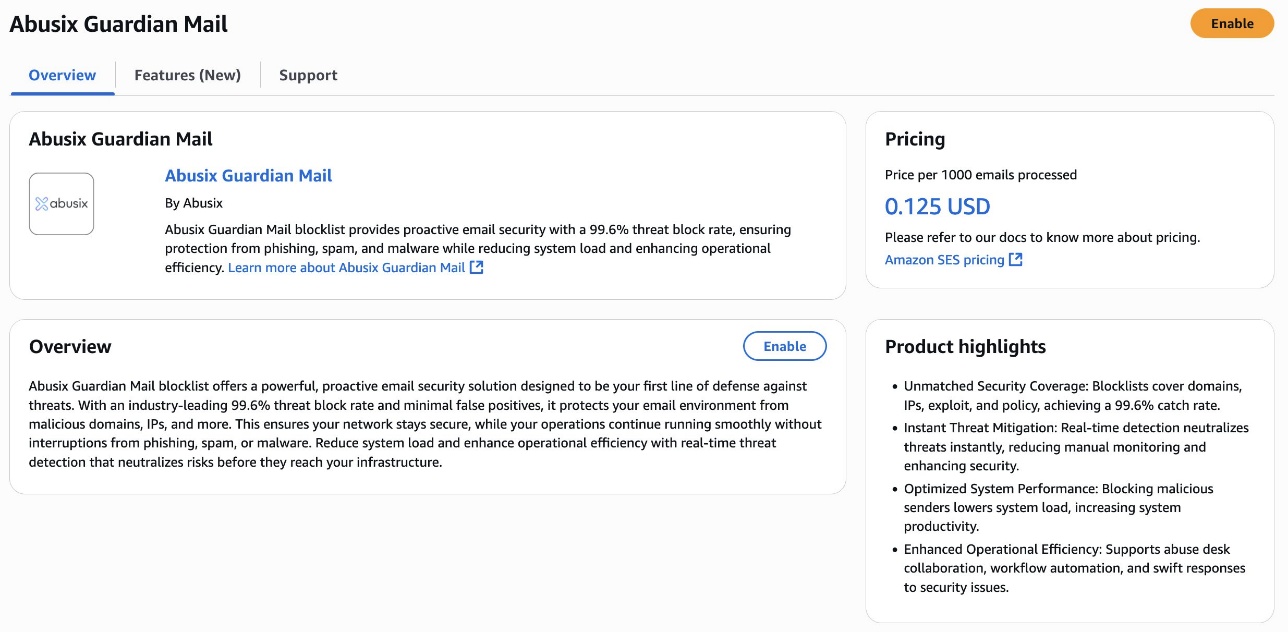
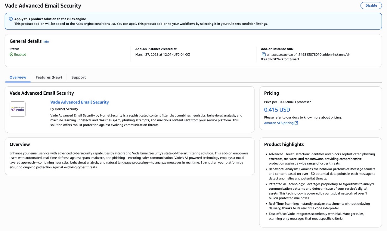

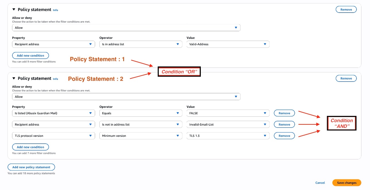
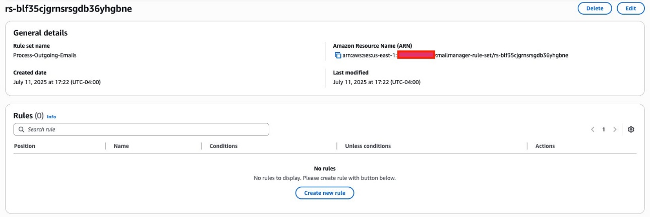
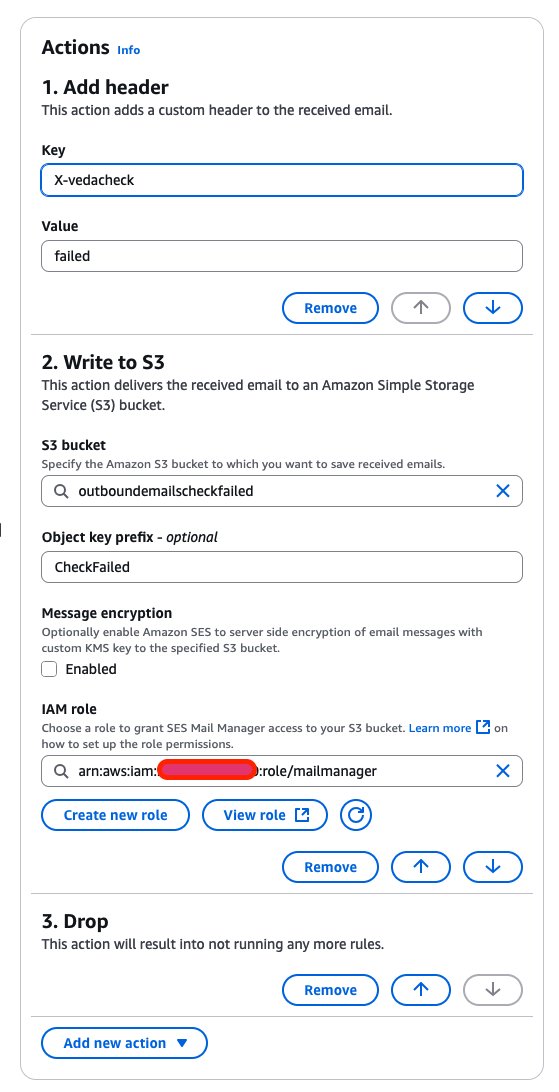
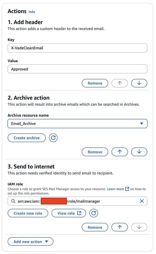
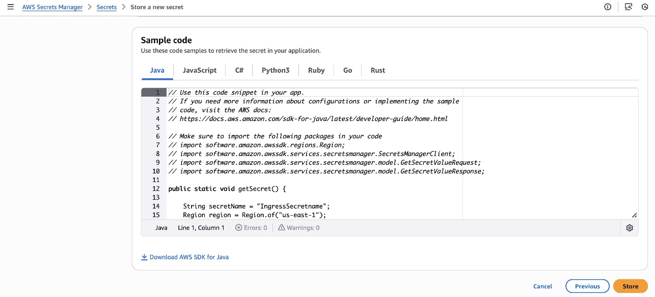
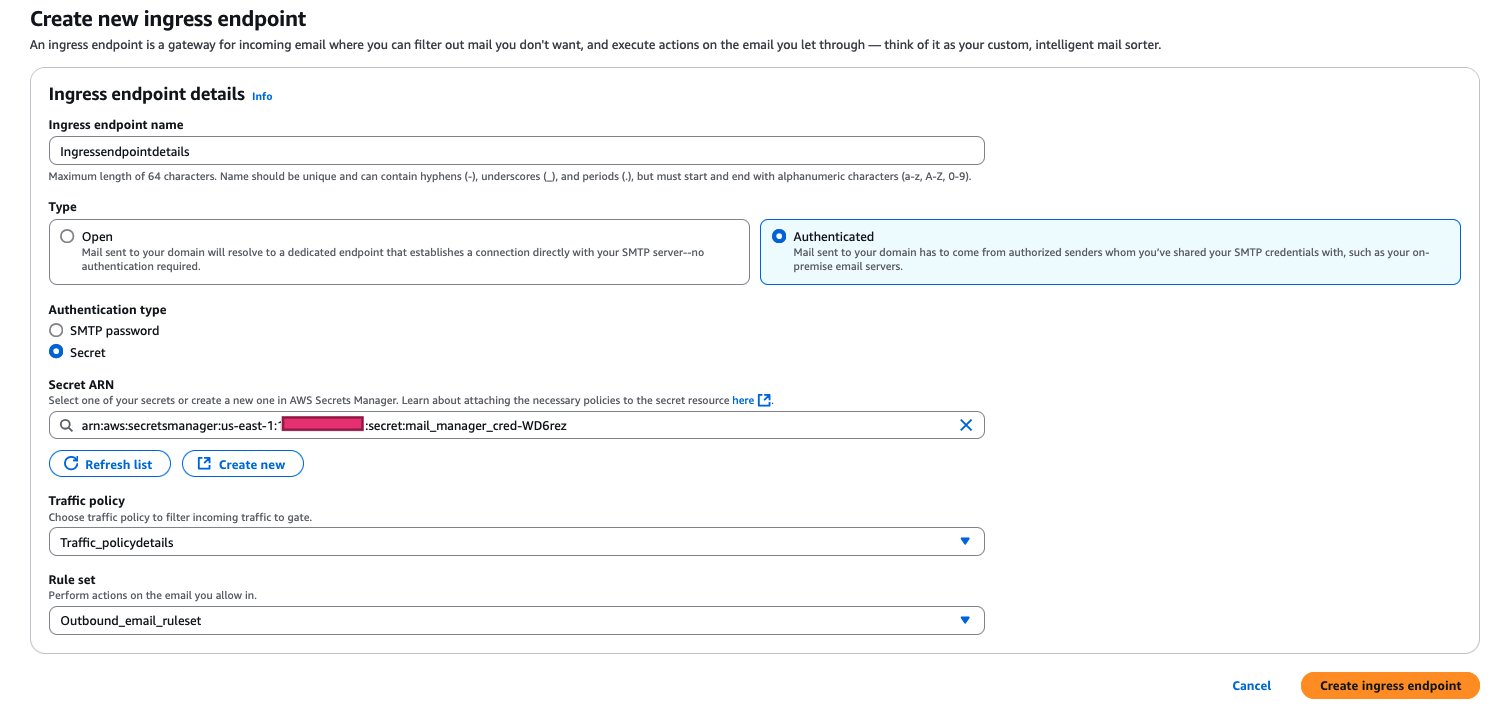 After your ingress endpoint is created, note down the following details from the General details section: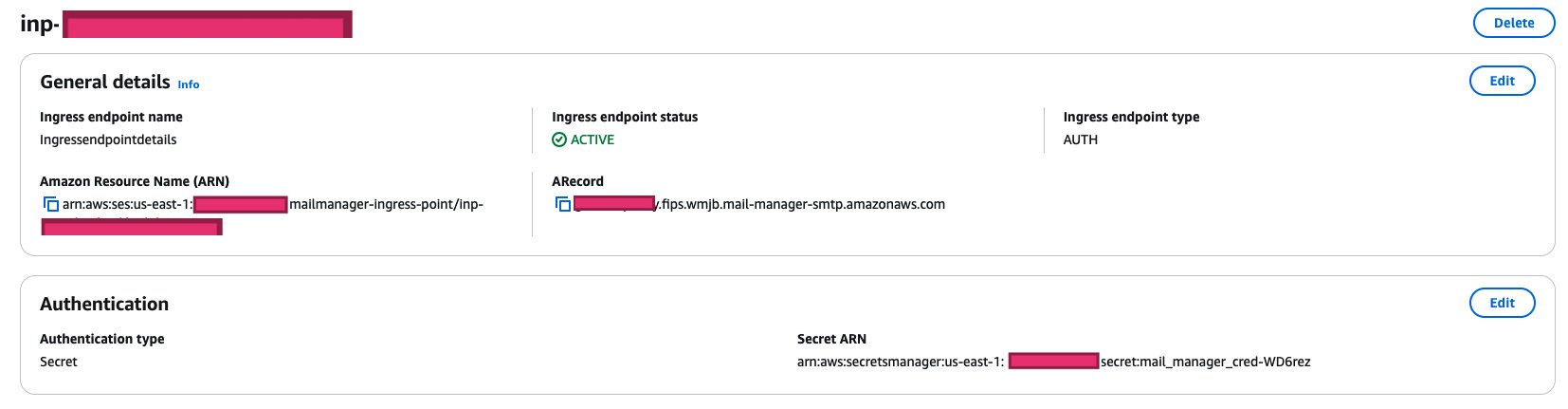
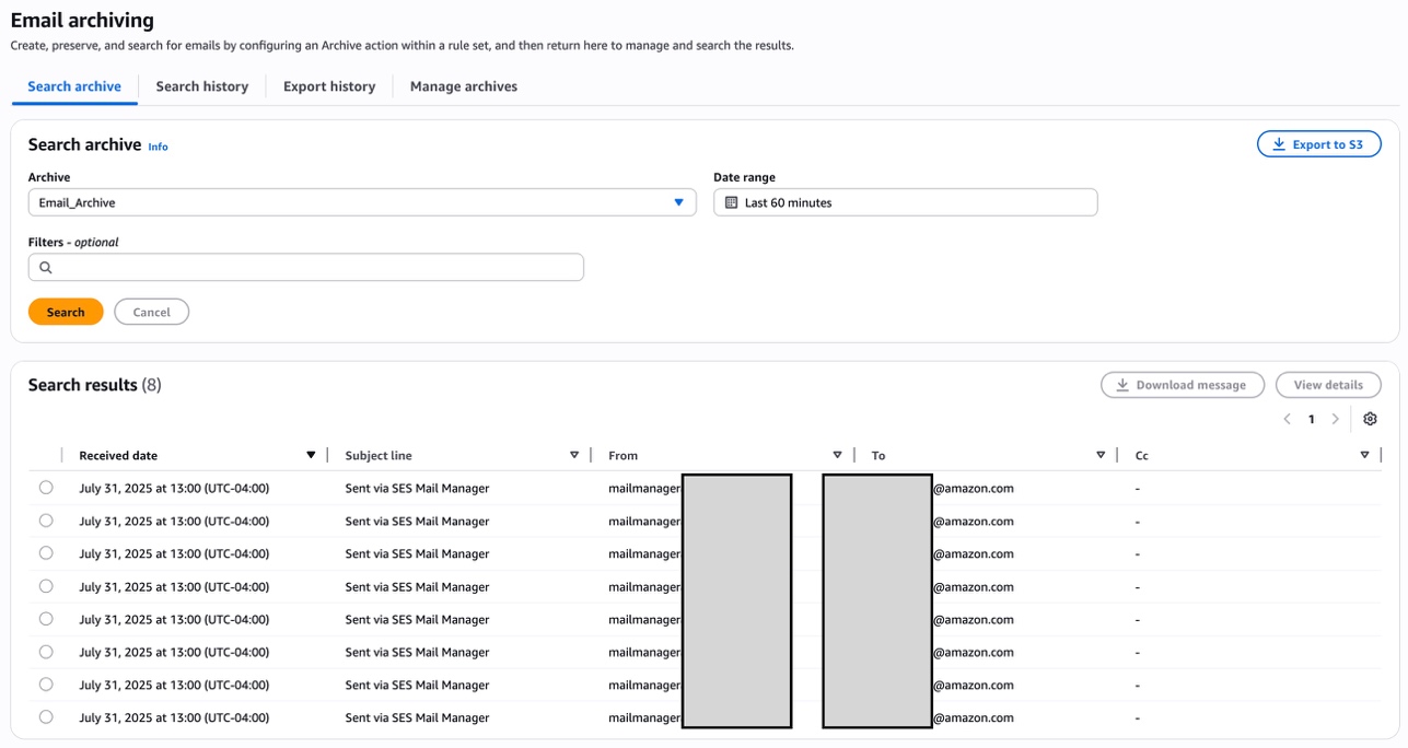
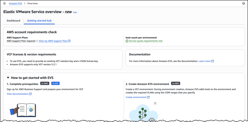
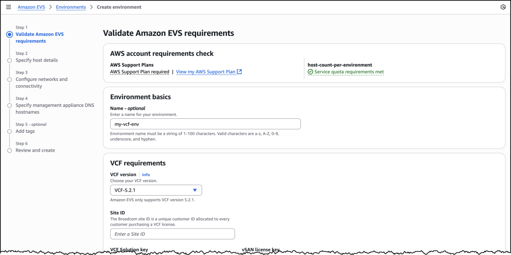
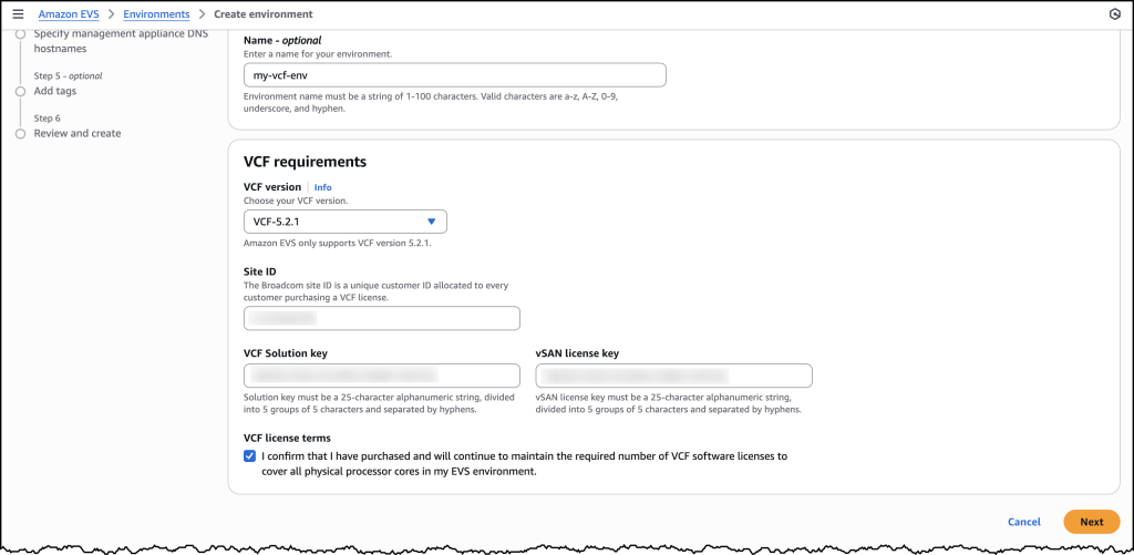
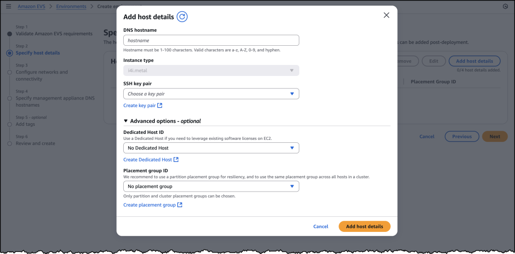
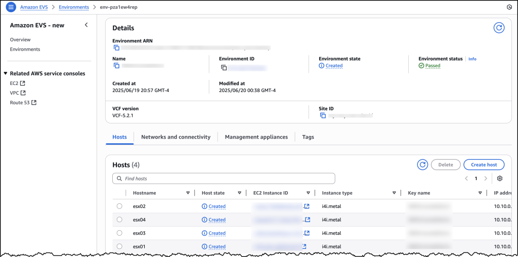
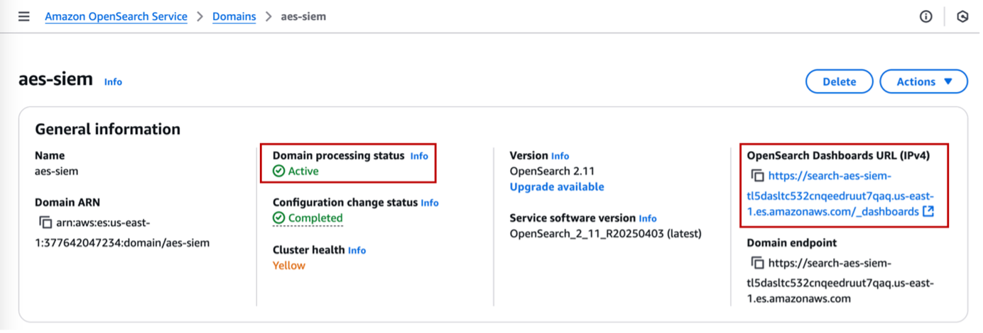
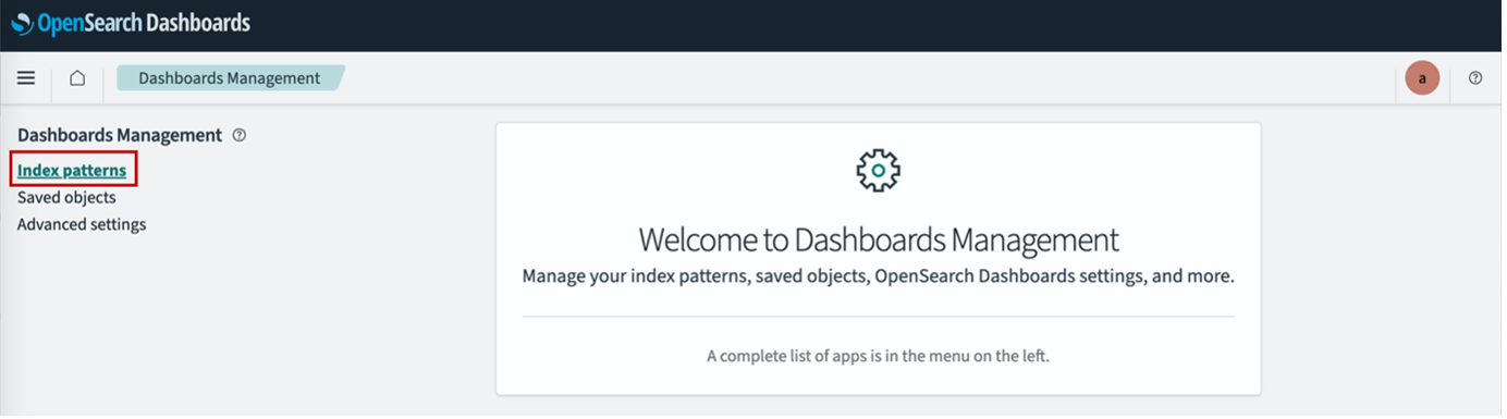
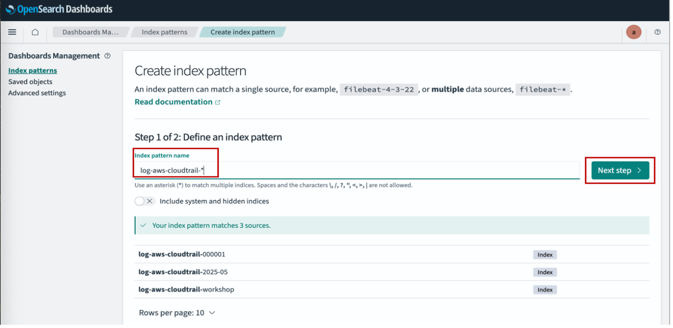
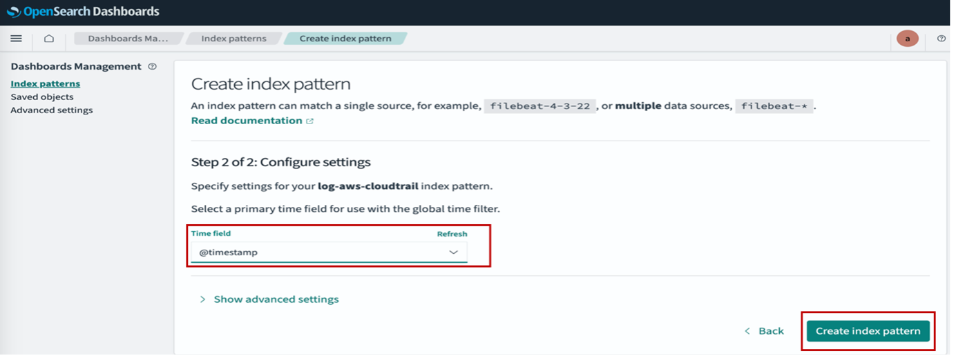
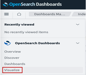
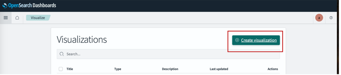
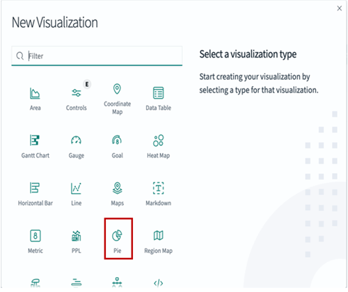
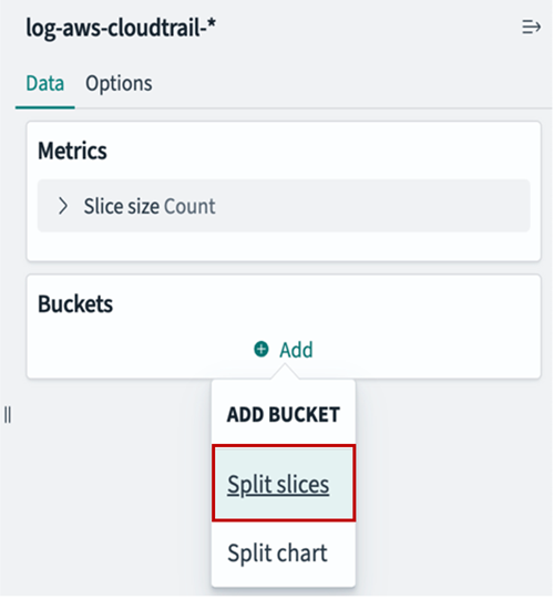
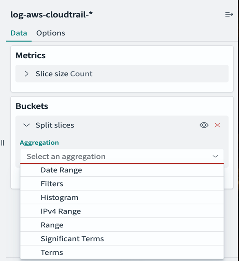
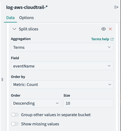
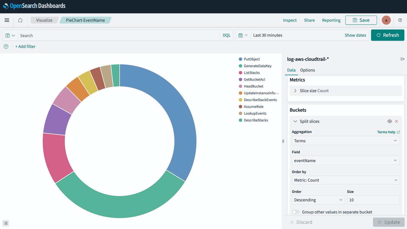
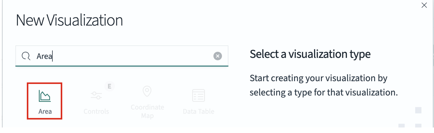
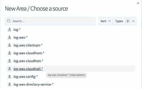
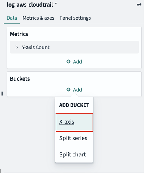
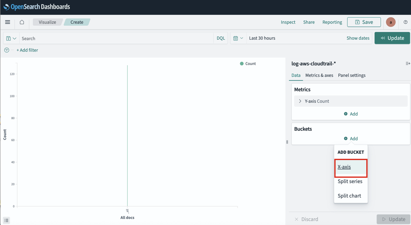
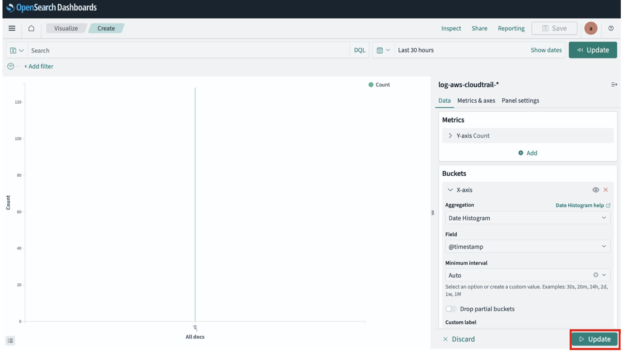
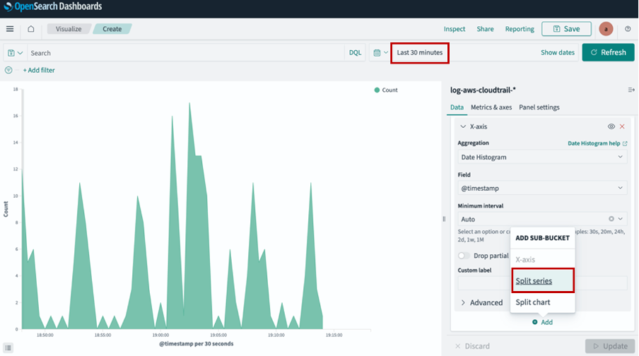
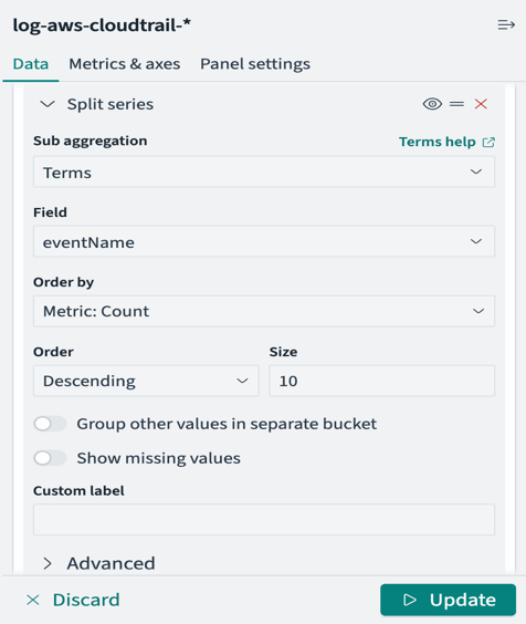
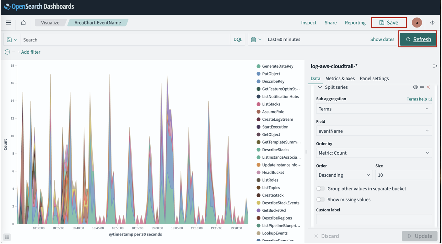
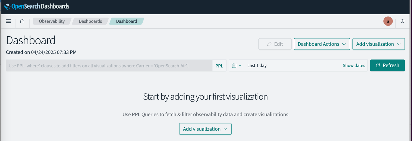
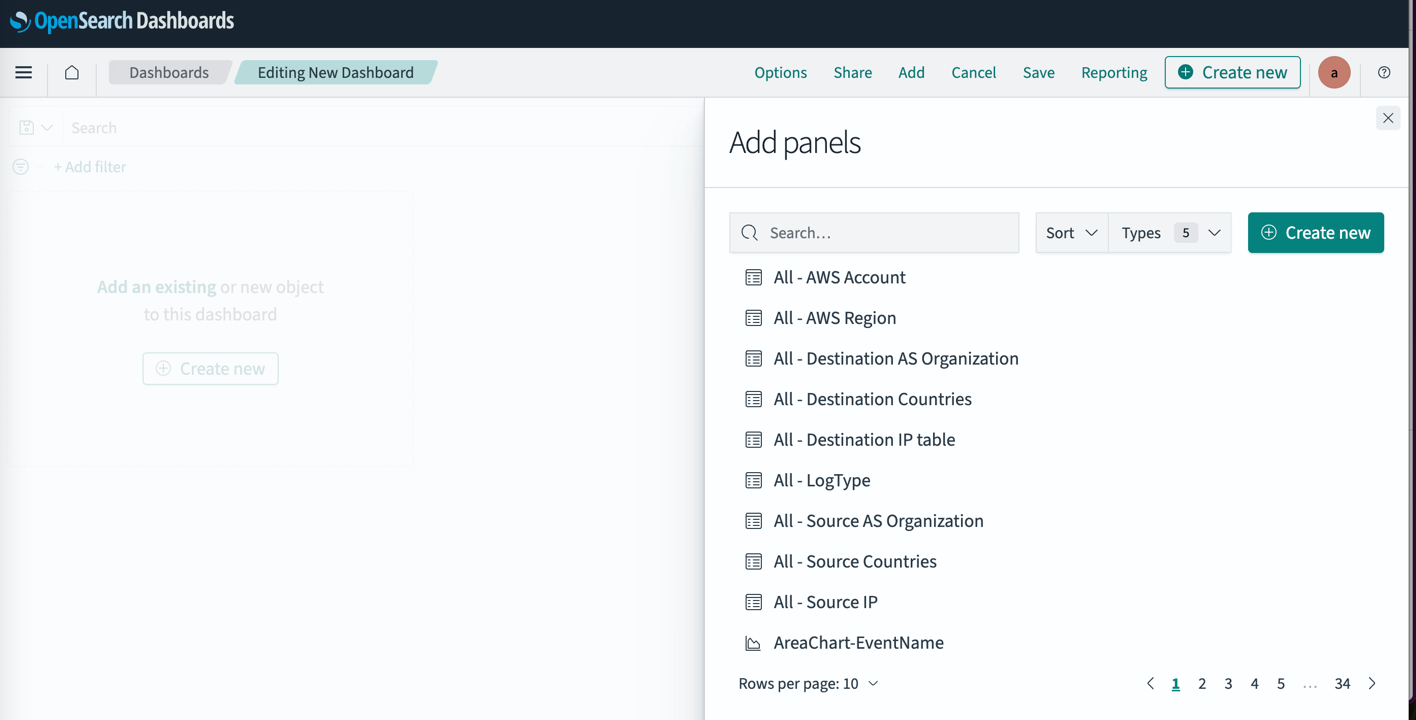
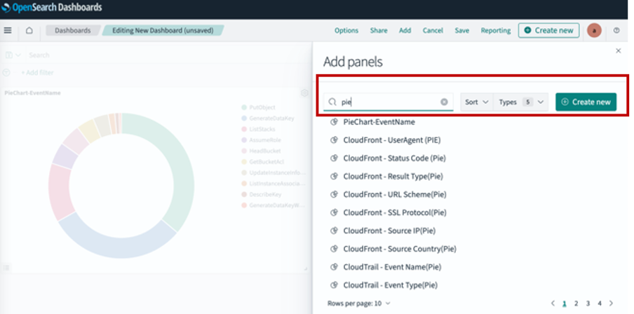
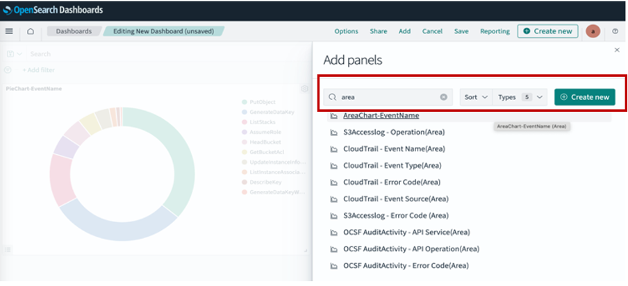
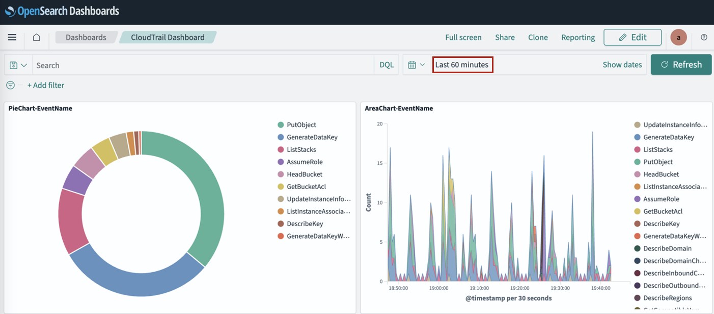
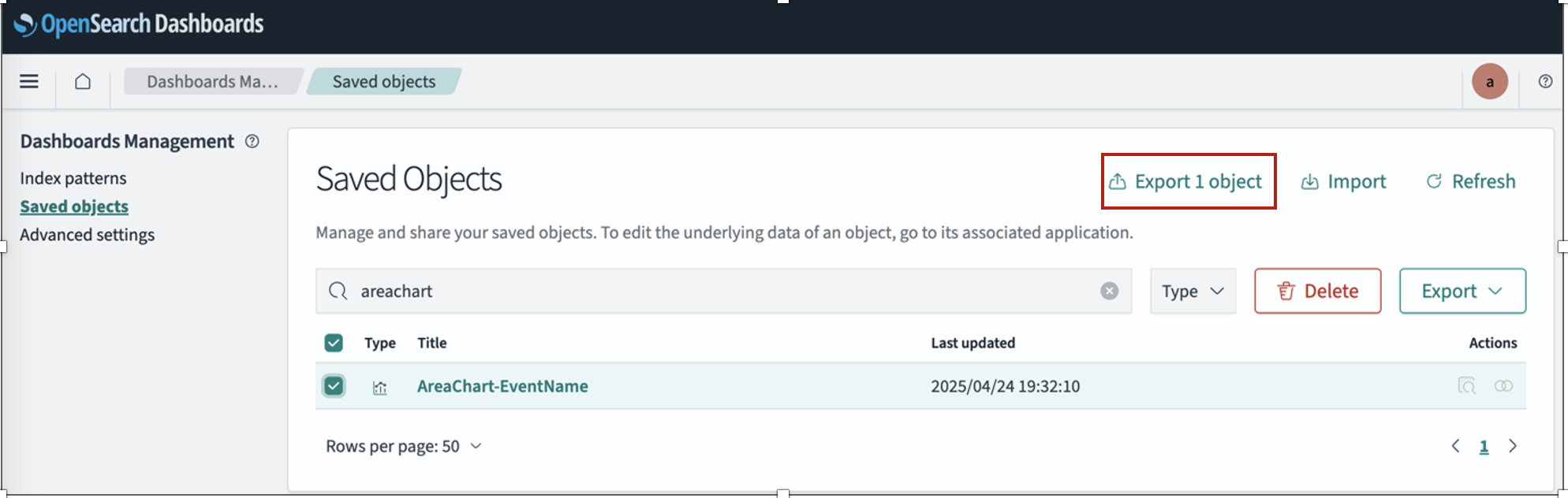
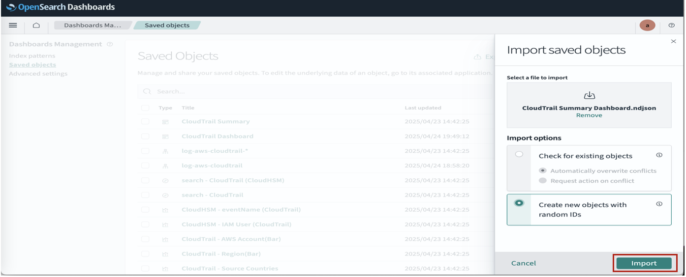
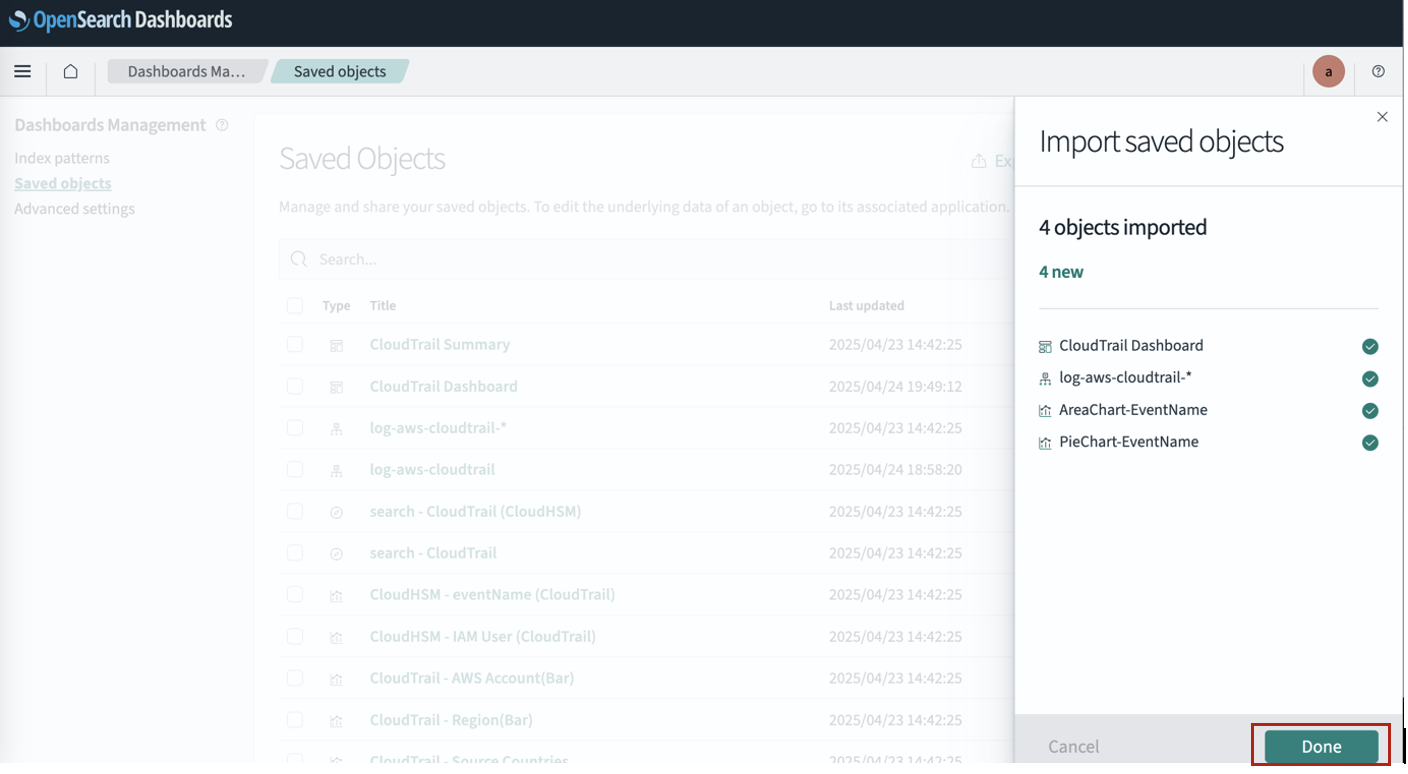
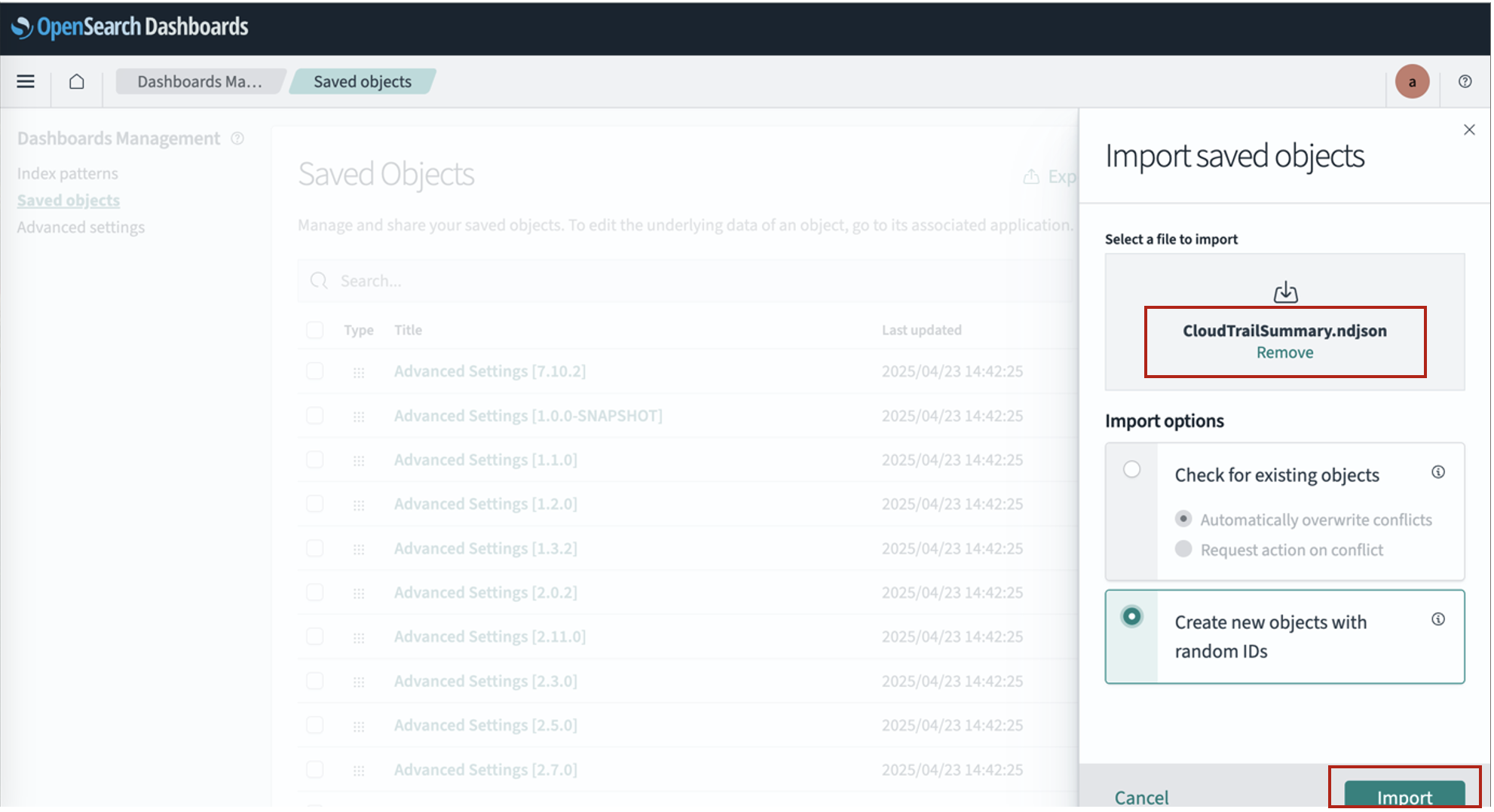
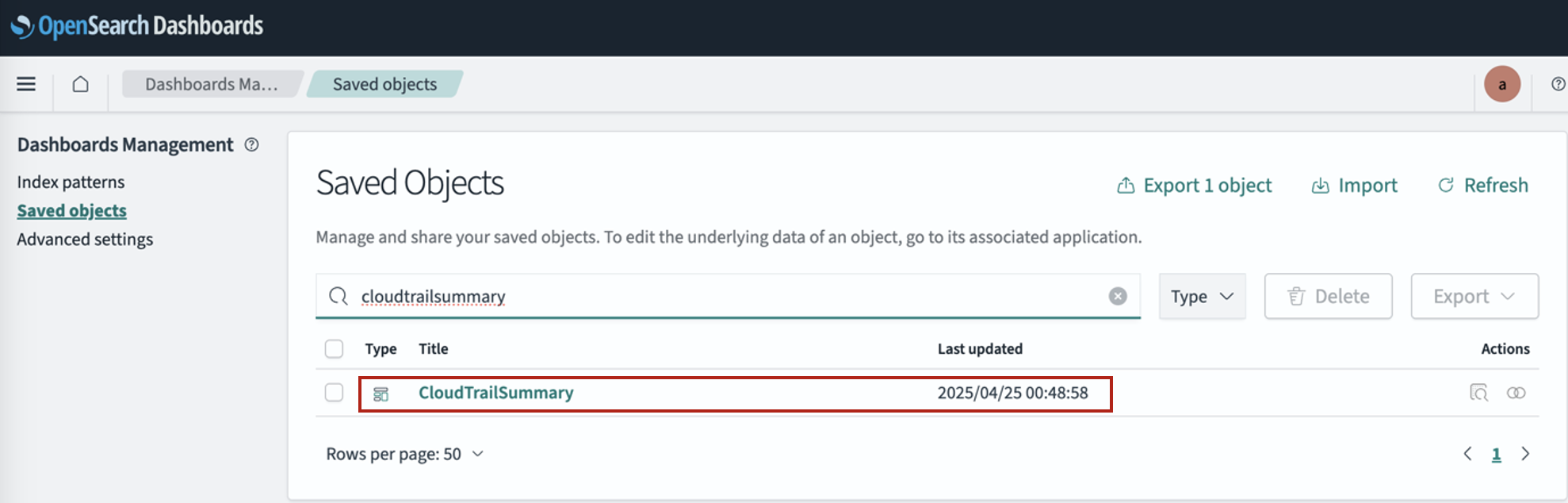
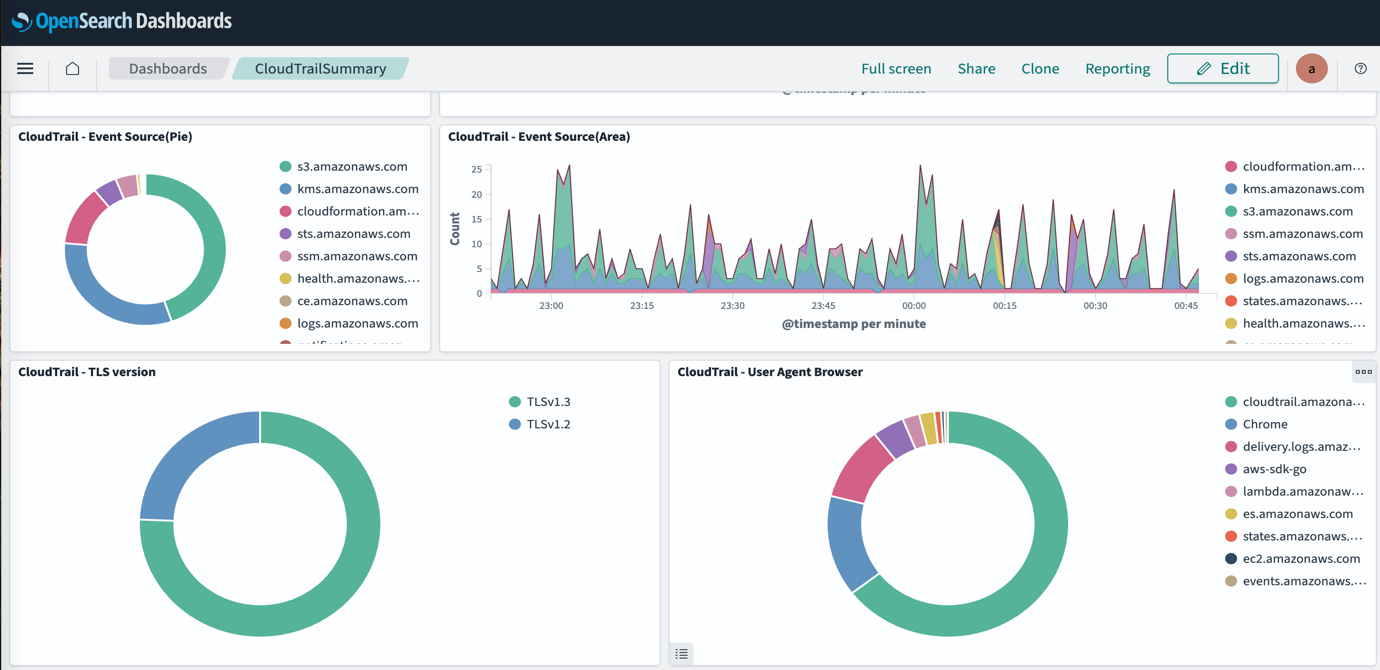
 Smita Singh is a Senior Solutions Architect at AWS. She focuses on defining technical strategic vision and works on architecture, design, and implementation of modern, scalable platforms for large-scale global enterprises and SaaS providers. She is a data, analytics, and generative AI enthusiast and is passionate about building innovative, highly scalable, resilient, fault-tolerant, self-healing, multi-tenant platform solutions and accelerators.
 Dipayan Sarkar is a Specialist Solutions Architect for Analytics at AWS, where he helps customers modernize their data platform using AWS analytics services. He works with customers to design and build analytics solutions, enabling businesses to make data-driven decisions.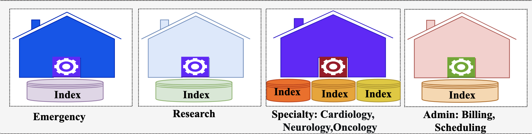
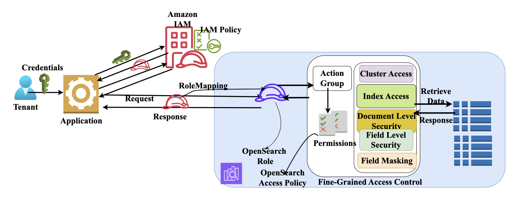
 Ezat Karimi is a Senior Solutions Architect at AWS, based in Austin, TX. Ezat specializes in designing and delivering modernization solutions and strategies for database applications. Working closely with multiple AWS teams, Ezat helps customers migrate their database workloads to the AWS Cloud.
 Jon Handler is a Senior Principal Solutions Architect at Amazon Web Services based in Palo Alto, CA. Jon works closely with OpenSearch and Amazon OpenSearch Service, providing help and guidance to a broad range of customers who have vector, search, and log analytics workloads that they want to move to the AWS Cloud. Prior to joining AWS, Jon’s career as a software developer included 4 years of coding a large-scale, ecommerce search engine. Jon holds a Bachelor’s of the Arts from the University of Pennsylvania, and a Master’s of Science and a PhD in Computer Science and Artificial Intelligence from Northwestern University.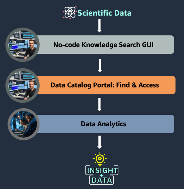
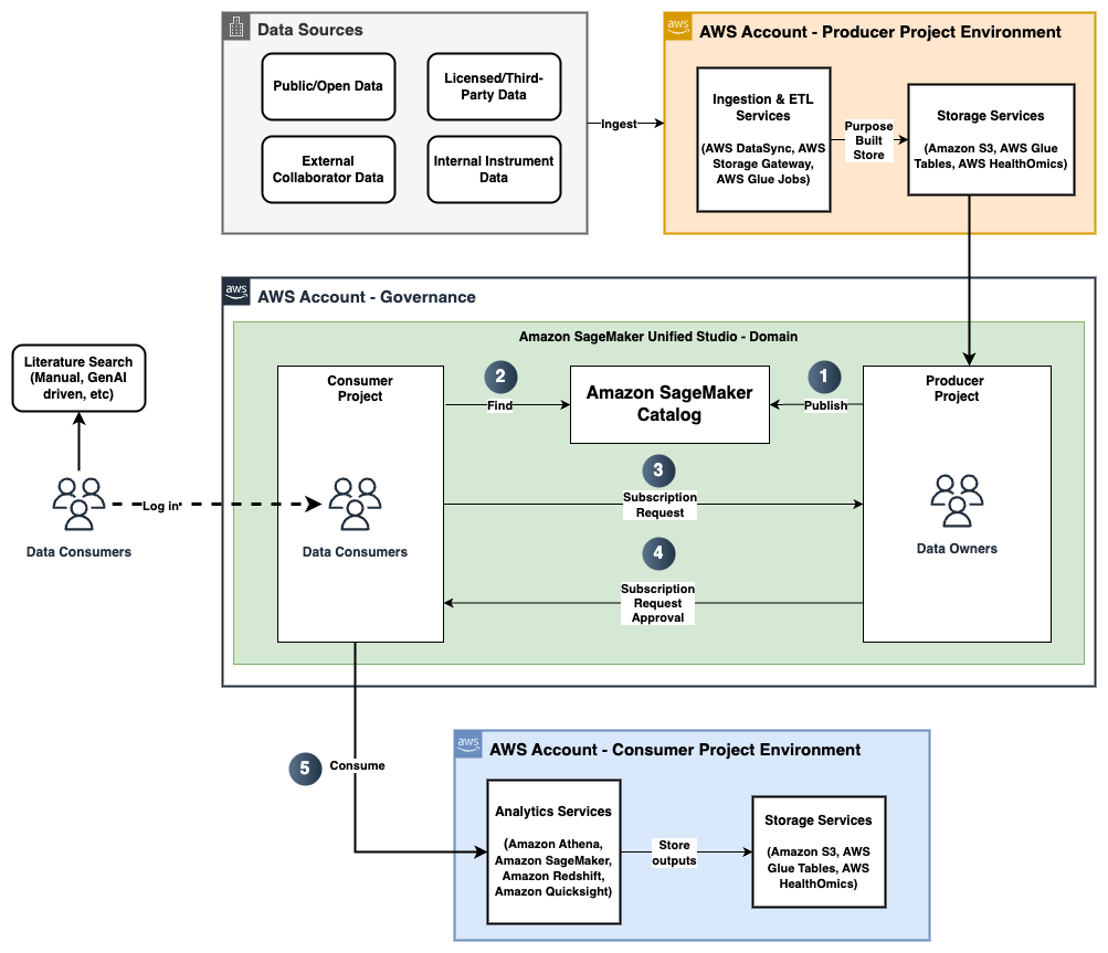
 Nadeem Bulsara is a Principal Solutions Architect at AWS specializing in Genomics and Life Sciences. He brings his 13+ years of Bioinformatics, Software Engineering, and Cloud Development skills as well as experience in research and clinical genomics and multi-omics to help Healthcare and Life Sciences organizations globally. He is motivated by the industry’s mission to enable people to have a long and healthy life.
 Chaitanya Vejendla is a Senior Solutions Architect specialized in DataLake & Analytics primarily working for Healthcare and Life Sciences industry division at AWS. Chaitanya is responsible for helping life sciences organizations and healthcare companies in developing modern data strategies, deploy data governance and analytical applications, electronic medical records, devices, and AI/ML-based applications, while educating customers about how to build secure, scalable, and cost-effective AWS solutions. His expertise spans across data analytics, data governance, AI, ML, big data, and healthcare-related technologies.
 Dr. Mileidy Giraldo has over 20 years of experience bridging bioinformatics, research, and industry technology strategy. She specializes in making technology accessible for organizations in the life sciences sector. In her current role as WW Lead for Life Sciences Strategy and Lab of the Future at AWS, she helps biotechs, biopharma, and diagnostics organizations design Data & AI-driven initiatives that modernize labs and help scientists unlock the full value of their data.
 Chris Clark is a Senior Solutions Architect focused on helping Life Science customers leverage AWS technology to advance their operational capabilities. With 20+ years of hands-on experience in life sciences manufacturing and supply chain, he combines deep industry knowledge with his AWS expertise to guide his customers. When he’s not working to solve customer challenges, he enjoys cycling and building and repairing things in his workshop.
 Nick Furr is a Specialist Solutions Architect at AWS, supporting Data & Analytics for Healthcare and Life Sciences. He helps providers, payers, and life sciences organizations build secure, scalable data platforms to drive innovation and improve outcomes. His work focuses on modernizing data strategies through cloud analytics, governed data processing, and machine learning for use cases like clinical research and population health.
 Subrat Das is a Principal Solutions Architect for Global Healthcare and Life Sciences accounts at AWS. He is passionate about modernizing and architecting complex customers workloads. When he’s not working on technology solutions, he enjoys long hikes and traveling around the world.