Post Syndicated from The Atlantic original https://www.youtube.com/watch?v=xKj8hHPy40w
Atlantic Reads: Abundance | The Atlantic Festival 2025
Post Syndicated from The Atlantic original https://www.youtube.com/watch?v=FZvkldRSxMs
AI and the Shifting Defense Landscape | The Atlantic Festival 2025
Post Syndicated from The Atlantic original https://www.youtube.com/watch?v=o9tpLx4-iWo
State of Our Union: How National Policies Impact Local Communities | The Atlantic Festival 2025
Post Syndicated from The Atlantic original https://www.youtube.com/watch?v=Y3jeTmRzOwU
Kingdoms United
Post Syndicated from The History Guy: History Deserves to Be Remembered original https://www.youtube.com/watch?v=fbUfX3wbpq0
Comic for 2025.05.02 – Captain Pills
Post Syndicated from Explosm.net original https://explosm.net/comics/captain-pills
New Cyanide and Happiness Comic
Unstoppable Force and Immovable Object
Post Syndicated from xkcd.com original https://xkcd.com/3084/

Intel Foundry Thermal Capabilities with TIM Options and In-Package Liquid Cooling Shown
Post Syndicated from Cliff Robinson original https://www.servethehome.com/intel-foundry-thermal-capabilities-with-tim-options-and-in-package-liquid-cooling-shown/
At this week’s 2025 Intel Foundry event, the company showed off its thermal capabilities with different TIM and co-packaged liquid-cooling
The post Intel Foundry Thermal Capabilities with TIM Options and In-Package Liquid Cooling Shown appeared first on ServeTheHome.
America’s Economic Forecast | The Atlantic Festival 2025
Post Syndicated from The Atlantic original https://www.youtube.com/watch?v=qUhzmCxTp5k
HHS & DOGE #lastweektonight
Post Syndicated from LastWeekTonight original https://www.youtube.com/watch?v=6v1gF49rb1M
AWS Lambda introduces tiered pricing for Amazon CloudWatch logs and additional logging destinations
Post Syndicated from Shridhar Pandey original https://aws.amazon.com/blogs/compute/aws-lambda-introduces-tiered-pricing-for-amazon-cloudwatch-logs-and-additional-logging-destinations/
Effective logging is an important part of an observability strategy when building serverless applications using AWS Lambda.
Lambda automatically captures and sends logs to Amazon CloudWatch Logs. This allows you to focus on building application logic rather than setting up logging infrastructure and allows operators to troubleshoot failures and performance issues more easily.
On May 1st, 2025, AWS announced changes to Lambda logging, which can reduce Lambda CloudWatch logging costs and make it easier and more cost-effective to use a wider range of monitoring tools. Lambda logs are now available at volume-based tiered pricing when using CloudWatch Logs Standard and Infrequent Access log classes. When generating Lambda logs at scale, you can expect an immediate cost reduction under this new pricing model. Lambda also now supports Amazon S3 and Amazon Data Firehose as additional destinations for Lambda logs, in addition to CloudWatch Logs. Lambda logs sent to S3 and Firehose are also available at volume-based tiered pricing.
This blog post covers some recent Lambda logging enhancements and describes how this change delivers a simpler, more cost-effective logging experience for Lambda.
Overview
Logging provides developers and operators with valuable data for debugging and troubleshooting application behavior, performance issues, and potential failures. It becomes even more important for serverless applications built using Lambda because of the ephemeral and stateless nature of the Lambda execution environment. Lambda’s built-in integration with CloudWatch Logs ensures that logs for every function invocation are readily available for analysis. The captured log data includes application logs generated by your Lambda function code and system logs generated by the Lambda service while running your function code. CloudWatch Logs allows you to search, filter, and analyze log data to troubleshoot issues, track metrics, and set up alerts.
Logging requirements evolve as serverless applications grow in complexity and scale, sometimes spanning hundreds or thousands of Lambda functions which generate substantial log volumes. Organizations need sophisticated logging solutions that can handle this scale while remaining cost-effective. Some scenarios—such as monitoring critical business transactions—demand real-time log analysis, while others focus on after-the-fact forensic analysis. Debug logs from development and staging environments often need high granularity, whereas you may want lower verbosity in production logs to improve the signal-to-noise ratio.
Recent Lambda logging enhancements
In recent years, Lambda and CloudWatch Logs have expanded Lambda’s logging capabilities to meet the evolving needs of serverless applications. These capabilities provide deeper insights, greater control, and more cost-effective solutions to capture, process, and consume logs to enhancing the serverless observability experience. Lambda advanced logging controls gives developers control over log generation and content. These controls allow you to capture Lambda logs in JSON structured format. You don’t have to use logging libraries and customize log levels (INFO, DEBUG, WARN, ERROR) separately for application and system logs. This helps reduce logging costs by ensuring only necessary logs are generated while maintaining appropriate visibility across different environments. For example, you can set verbose DEBUG level logging in development environments while limiting production logging to ERROR level to improve the signal-to-noise ratio and control costs.
The Infrequent Access log class for CloudWatch Logs introduced a cost-effective solution for logs that need retention but are accessed less frequently. Infrequent Access is 50% lower per GB ingestion price than the Standard log class This tailored set of capabilities allows you to reduce your logging costs while maintaining access to historical data for compliance, audit purposes, or forensic analysis.
CloudWatch Logs Live Tail is an interactive, real-time log streaming and analytics capability. Live Tail streamlines debugging and monitoring workflows; it allows you to observe log output as functions execute without navigating away from the Lambda console. This makes it easier to identify and diagnose issues during development and troubleshooting. Logs Live Tail is also available in Visual Code IDE.
Tiered pricing for Lambda logs in CloudWatch Logs
Starting today, Lambda logs sent to CloudWatch Logs are classed as Vended Logs, which are logs from specific AWS services that are available at volume tiered pricing. This replaces the previous flat rate model when using CloudWatch Logs Standard log class. For example, in the US East (N. Virginia) AWS Region, you were charged at $0.50 per GB when using Standard log class for your Lambda logs. Under the new pricing model, you are charged for sending your Lambda logs to CloudWatch Logs starting at $0.50 per GB for initial usage. As log volume increases, the price per GB automatically decreases through multiple tiers, reaching rates as low as $0.05 per GB in the lowest tier. This pricing change applies automatically to all Lambda logs sent to CloudWatch Logs, requiring no code or configuration changes from you.
| Data Ingested | CloudWatch Logs Standard | CloudWatch Logs Infrequent Access |
| First 10 TB per month | $0.50 per GB | $0.25 per GB |
| Next 20 TB per month | $0.25 per GB | $0.15 per GB |
| Next 20 TB per month | $0.10 per GB | $0.075 per GB |
| Over 50 TB per month | $0.05 per GB | $0.05 per GB |
Table 1: Tiered pricing for Lambda logs in CloudWatch Logs in US East (N. Virginia) Region
When generating Lambda logs at scale, you will see an immediate cost reduction under this new pricing model. For example, if you generate 60 TB of Lambda logs monthly in CloudWatch Logs, costs would decrease by 58% (from $30,000 to $12,500). The pricing tiers scale with your logging volume, ensuring that cost benefits increase as your application grows. This allows you to maintain comprehensive logging practices that previously may have been cost-prohibitive. Vended logs tiered pricing is applied on all vended logs ingested to CloudWatch and not tiered per service.
When ingesting other vended logs, such as Amazon Virtual Private Cloud flow logs and Amazon Route 53 resolver query logs, you will see larger discounts as the tiering is applied at a consolidated log ingestion volume.
New Lambda logging destinations: Amazon S3 and Amazon Data Firehose
Starting today, Lambda also supports Amazon S3 and Amazon Data Firehose as destinations for Lambda logs, in addition to CloudWatch Logs. When using S3 or Firehose as a destination, logging costs start at $0.25 per GB. The tiered pricing also applies, with rates reducing to as low as $0.05 per GB in the lowest tier. This tiering is also applied at a consolidated log ingestion volume.
| Data Ingested | Delivery Cost to Amazon S3 | Delivery Cost to Amazon Data Firehose |
| First 10TB per month | $0.25 per GB | $0.25 per GB |
| Next 20TB per month | $0.15 per GB | $0.15 per GB |
| Next 20TB per month | $0.075 per GB | $0.075 per GB |
| Over 50TB per month | $0.05 per GB | $0.05 per GB |
Table 2:Tiered pricing for Lambda logs delivery to Amazon S3 and Amazon Data Firehose in US East (N. Virginia) Region
Direct delivery of Lambda logs to S3 provides enhanced flexibility in log management. Support for Firehose streamlines Lambda log delivery to additional destinations such as Amazon OpenSearch Service, HTTP endpoints, and third-party observability providers. This matches the established log delivery pattern used with other AWS compute services such as Amazon Elastic Container Service (Amazon ECS) and Amazon Elastic Compute Cloud (Amazon EC2).
This new capability provides significant cost benefits and streamlines log delivery to additional logging destinations, making it easier to use a wider range of monitoring tools (including CloudWatch) when building serverless applications using Lambda.
New Lambda logging destinations in action
All new and existing Lambda functions have CloudWatch Logs as the default logging destination, with S3 and Firehose as alternative choices. When you select S3 or Firehose as your logging destination, Lambda sends logs to the selected destination via a new CloudWatch Logs Delivery log class. This log class enables efficient routing but doesn’t support CloudWatch Logs Standard log class features, such as Logs Insights and Live Tail.
To set up S3 or Firehose as the destination for your Lambda logs in the Lambda console:
- Navigate to the Lambda console, and select or create a function to set up an S3 or Firehose logging destination.
- In the Configuration tab, select Monitoring and operations tools on the left pane.
- Select Edit in the Logging configuration. This opens the Edit logging configuration page.

Figure 1. Edit logging configuration in Lambda console
- In the Log destination section, select Amazon S3 or Amazon Data Firehose. Amazon CloudWatch Logs is the default selection.

Figure 2. Select log destination in the Edit logging configuration page
- Under CloudWatch delivery log group, choose Create new log group or Existing log group.
- To create a new delivery log group to send logs to S3, enter a log group name and specify the destination S3 bucket. Provide an AWS Identity and Access Management (IAM) role for CloudWatch Logs to deliver logs to S3.
Follow similar steps to send logs to a Firehose stream.
Figure 3. Create new CloudWatch delivery log group for S3
- To use an existing delivery log group, select one from the Delivery log group. The selected delivery log group must have a configured destination (S3 or Firehose) and match the destination you selected.

Figure 4. Select existing CloudWatch delivery log group for Firehose


Advanced logging controls are also available for S3 and Firehose destinations. These controls include JSON structured format selection and log level filters for both application and system logs. This gives you enhanced log management controls for easier search, filter, and analysis. You can also use AWS Command Line Interface (AWS CLI) and infrastructure as code (IaC) tools such as AWS CloudFormation and AWS Cloud Development Kit (AWS CDK) to set up Lambda logs delivery to S3 and Firehose.
Best practices
To get the most out of the changes announced today, ensure that your logging strategy is closely aligned with the requirements of your workload. For example, consider sending critical production logs to CloudWatch Logs to take advantage of its advanced real-time analytics and alerting features. You now automatically benefit from volume-based discounts through tiered pricing in CloudWatch Logs for high-volume logging scenarios. For logs that need long-term retention for historical analysis, you can use S3’s storage classes to further reduce costs. When using your existing or third-party monitoring tools, direct integration through Firehose eliminates the need for custom forwarding solutions and associated costs.
Logging cost optimization extends beyond destination selection. Monitor log volumes regularly to understand the impact of pricing tiers. Implement appropriate retention policies to prevent unnecessary storage of old logs and log sampling for high-volume debug logs. Consider using different logging strategies across development, staging, and production environments to balance observability needs with cost efficiency.
Conclusion
Tiered pricing for Lambda logs in CloudWatch Logs and support for S3 and Firehose as additional logging destinations improves Lambda application observability. You can now manage logging costs at scale and expand Lambda monitoring solutions through cost-effective, easy-to-configure integrations. Whether you’re building new serverless applications or optimizing existing ones, these enhancements help you implement comprehensive logging strategies that scale cost-effectively with your workload.
The new features announced today are available in all commercial AWS Regions where Lambda and CloudWatch Logs are available. Support for configuring log delivery to S3 and Firehose in the Lambda console is available in US East (Ohio), US East (N. Virginia), US West (Oregon), and Europe (Ireland) Regions, with additional Regions coming soon. Review the Lambda documentation and CloudWatch Logs documentation to learn more about these features and how to use them. Review the CloudWatch pricing page to learn more about how these features are priced.
For more serverless learning resources, visit Serverless Land.
Can the Nexigo Aurora Pro MKII Beat the Hisense PX3-Pro and Formovie Theater Premium?
Post Syndicated from The Hook Up original https://www.youtube.com/watch?v=90mdBtMSuoI
Redis is now available under the AGPLv3 open source license (Redis blog)
Post Syndicated from jake original https://lwn.net/Articles/1019686/
After a somewhat tumultuous switch to the
Server Side Public License (SSPL) in March 2024, Redis has backtracked
and is now offering Redis under the
Affero GPLv3 (AGPLv3) starting with Redis 8, CEO Rowan Trollope
announced. The change back to an open-source license was led by Redis creator Salvatore
“antirez” Sanfillipo, who also contributed the new Vector Sets feature for
the release. He said:
I’ll be honest: I truly wanted the code I wrote for the new Vector Sets data type to be released under an open source license. Writing open source software is too rooted in me: I rarely wrote anything else in my career. I’m too old to start now. This may be childish, but I wrote Vector Sets with a huge amount of enthusiasm exactly because I knew Redis (and my new work) was going to be open source again.
I understand that the core of our work is to improve Redis, to continue building a good system, useful, simple, able to change with the requirements of the software stack. Yet, returning back to an open source license is the basis for such efforts to be coherent with the Redis project, to be accepted by the user base, and to contribute to a human collective effort that is larger than any single company. So, honestly, while I can’t take credit for the license switch, I hope I contributed a little bit to it, because today I’m happy. I’m happy that Redis is open source software again, under the terms of the AGPLv3 license.
Since last year’s license switch, though, the Valkey project has sprung up as a fork under
the original 3-clause BSD license.
Iceberg on Backblaze B2
Post Syndicated from Pat Patterson original https://www.backblaze.com/blog/iceberg-on-backblaze-b2/
If you work with cloud storage and data lakes, you’re likely hearing the word “Iceberg” with increasing frequency, occasionally prefixed by “Apache”. What is Apache Iceberg, and how can you leverage it to efficiently store data in object stores such as Backblaze B2 Cloud Storage? I’ll answer both of those questions in this blog post.
But, first, join me on a brief trip back in time to the beginning of the twenty-first century, a long-ago time before the emergence of big data and cloud computing.
A timely shoutout to the Data Council conference
We recently attended the 2025 Data Council conference and caught Ryan Blue, co-creator of Apache Iceberg’s excellent presentation (featuring some very entertaining slides).
If you want to hear more about topics like this one, feel free to join us at Backblaze Weekly, an ongoing webinar series where we discuss all things Backblaze.

CSV: The lingua franca of tabular data
In the early 2000s, if you were working with tabular data, you were likely using either a relational database management system (RDBMS), such as Oracle Database, or a spreadsheet, likely Microsoft Excel.
Data stored in an RDBMS is highly structured, meaning that it MUST conform to a predefined schema. For example, you might create an employee table with columns such as first name, last name, date of birth, hire date, and so on. The database schema holds metadata such as the name and data type of each column, whether that column must have a value, relationships between tables, and so on.
A spreadsheet, on the other hand, has some structure—data is arranged in rows and columns, similarly to an RDBMS–but each cell can contain anything: text, a number, a formula referencing other cells, even an image in today’s spreadsheets. We say that a spreadsheet is semi-structured data.
At the turn of the century, each database and spreadsheet had its own proprietary file format, optimized for its own requirements, and often not at all publicly documented, but the need to be able to exchange data between applications led to broad adoption of a file format to allow just that: comma-separated values, or CSV.
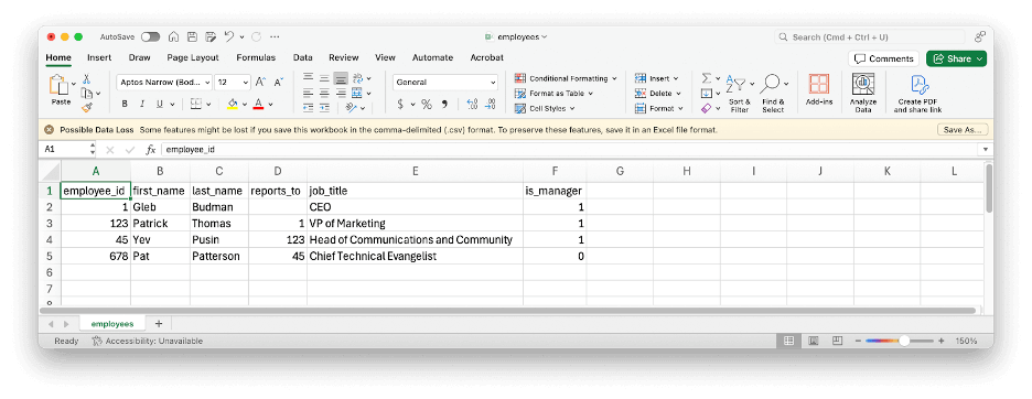
Here’s a simple example of some tabular data represented as CSV:
employee_id,first_name,last_name,reports_to,job_title,is_manager
1,Gleb,Budman,,CEO,1
123,Patrick,Thomas,1,"VP of Marketing",1
45,Yev,Pusin,123,"Head of Communications and Community",1
678,Pat,Patterson,45,"Chief Technical Evangelist",0
CSV is simple and flexible enough that it was easy for me to type that example up manually and import it into Microsoft Excel with no problems at all. Note that, as well as the commas, the double quotes in the CSV data are part of the file format, and do not appear in the imported data:
CSV has a lot of advantages: It’s simple; flexible; widely understood; the optional header line means that data can be somewhat self-describing; and it’s not controlled by any single vendor.
CSV does, however, also have a few disadvantages, including:
- There’s no schema; nothing in that file expresses that the values in the first column, apart from the header, must be integers.
- It’s difficult to represent complex or hierarchical datasets.
- Data is stored as text, which is inefficient for numerical and repetitive data. Text representations of numbers occupy more storage than binary, and applications must convert them to binary when loading the file and convert them back to text when saving it.
Avro, Parquet and ORC: File formats for big data
The emergence of open-source distributed computing frameworks such as Apache Hadoop and, later, Apache Spark, in the first two decades of this century drove the creation and adoption of more efficient ways of storing tabular data. Avro, Parquet and ORC, all Apache projects, are binary file formats that address shortcomings of CSV, such as encapsulating schema alongside the data.
Avro, like CSV, is designed for row-oriented data, which makes it well-suited to use cases that involve appending new data to files. Parquet and ORC, in contrast, are column-oriented file formats, perfect for online analytical processing (OLAP) use cases where, for example, an application might read an entire column from a table to calculate the sum of its values. As well as storing numbers in a binary representation, Parquet and ORC can also reduce file size through compression strategies such as run-length encoding.
Here’s a concrete example: The Drive Stats data set for December 2024 occupies 3.7GB of storage in CSV format. As Parquet, the same data consumes just 242MB, a data compression ratio of more than 15:1.
Why does it matter if your dataset is smaller? Well, beyond just cost savings, which are amplified when dealing with huge datasets, smaller files mean that running queries against full datasets takes less time, which reduces server load, compute costs, and so on.
From file formats to table formats and data lakes
Apache Hadoop’s original use case was as an implementation of MapReduce, a programming model for manipulating large datasets. Engineers at Facebook, tasked with allowing SQL queries over datasets generated by Hadoop, created Apache Hive, and, with it, the Hive table format, which specified how to view a collection of files as a single logical table. The Hive table format in turn allowed organizations to create data lakes, repositories that store structured and semi-structured data in their original format for analysis by a wide range of tools, and, later, data lakehouses, which aim to combine the benefits of data lakes and traditional data warehouses by storing structured data using data lake tools and technologies.
A key concept of the Hive table format is partitioning, a way of organizing files to reduce the amount of data that must be read to process a query. Taking the Drive Stats dataset as an example, we can partition the files by year and month, so that each file has a prefix of the form:
/drivestats/year={year}/month={month}/
For example:
/drivestats/year=2024/month=12/
With this partitioning scheme, a system processing a query for hard drive statistics for, say, December 12, 2024, need only retrieve files with the above prefix. You might be wondering, “Why not partition the data on day, also, to further reduce the number of files that must be retrieved?” The answer depends on the data volume and access patterns. It’s much more efficient to partition data into fewer large files than many small files, so overly granular partitioning can actually impair performance.
It’s worth mentioning that file formats and table formats are largely independent of each other. You can use Avro, Parquet, ORC, or even CSV files with the Hive table format.
For more detail on the Parquet file format, Hive table format, and partitioning, see the blog post, Storing and Querying Analytical Data in Backblaze B2.
“Iceberg, captain, dead ahead!”
While the Hive table format served the big data community well for several years, it had a number of shortcomings:
- Every query incurs a file list (“list objects”, in S3 API terms) operation, which is particularly expensive with cloud object storage, both in terms of time and API transaction charges.
- Deleting or modifying data typically implies rewriting an entire data file, even if only a single row was affected.
- Hive can only partition datasets on columns that are in the table schema. For example, the Drive Stats data set includes a
datecolumn, so to use it with Hive, we had to create additional, redundant,yearandmonthcolumns. - Any changes to the data schema or partitioning strategy require affected files to be rewritten, making schema evolution problematic, if not infeasible, for large datasets.
- There is limited support for the kind of ACID (Atomic, Consistent, Isolated, Durable) transactions that are familiar from the RDBMS world. Attempts to add transaction support to Hive were not widely or consistently supported.
As a result, vendors and the broader big data community formed a number of projects to define new table formats to succeed Hive, including Apache Iceberg, Apache Hudi, and Delta Lake, a Linux Foundation project.
The three are broadly comparable in terms of features, but, over the past couple of years, Iceberg has emerged as the leader in terms of vendor adoption, with Snowflake announcing general availability of Iceberg tables in June 2024, and Amazon announcing S3 Tables, its managed Iceberg offering, in December 2024. Significantly, Databricks, the prime mover behind Delta Lake, acquired Tabular, a company founded by the original creators of Apache Iceberg, in June 2024, establishing its own beachhead in the Iceberg community.
Iceberg‘s features allow it to be used to organize huge data sets, efficiently and flexibly:
- Table metadata including the list of files that comprise a table is stored as JSON data alongside the data files, eliminating the need to run an expensive list object operation for every query.
- Schema evolution allows you to add, drop, update, or rename columns.
- Hidden partitioning decouples partitioning from the table schema. For example, you can partition data like the Drive Stats dataset by year and month based on the existing date values, without creating additional columns.
- Partition layout evolution allows you to modify your partitioning strategy as data volume or access patterns change.
- Time travel allows you to query table snapshots.
- Serializable isolation provides atomic table changes, ensuring readers never see inconsistent data.
- Multiple concurrent writers use optimistic concurrency, retrying to ensure that compatible updates succeed while detecting conflicting writes.
Iceberg is widely supported across the big data ecosystem, with many applications and tools allowing you to store Iceberg tables in S3 compatible cloud object storage such as Backblaze B2. In this article, I’ll look at the simplest use case, running queries against the Drive Stats dataset, with three representative examples: Snowflake, Trino, and DuckDB.
Writing Iceberg data to Backblaze B2
I wrote a simple Python application, drivestats2iceberg, using the PyIceberg library, that converts the Drive Stats dataset from the zipped CSV files we publish to Parquet files in an Iceberg table stored in a Backblaze B2 Bucket. There are some useful techniques in drivestats2iceberg, and it is published on GitHub as open source, under the MIT license, so feel free to use it as a starting point for your own data conversion apps.
Querying Iceberg tables in Backblaze B2 from Snowflake
Snowflake is a data-as-a-service platform addressing a wide variety of use cases, including artificial intelligence (AI), machine learning (ML), collaboration across organizations, and data lakes.
As I mentioned above, Snowflake announced general availability of its Iceberg tables offering in June 2024, allowing you to manipulate Iceberg tables located on external volumes, outside your Snowflake warehouse, and query them alongside data in Snowflake-managed tables.
Snowflake’s Iceberg implementation is quite complicated, with different capabilities according to your choice of cloud object storage provider and whether you want Snowflake to manage your Iceberg catalog or use a catalog integration.
For our simple use case, where the Iceberg metadata and data files already exist in a Backblaze B2 Bucket, the first step is to create a Snowflake external volume, configuring it with suitable credentials and the location of the Drive Stats data.
Note: the application key shown in this Snowflake statement has read-only access to the drivestats-iceberg bucket. You can use it to query the Drive Stats data set from your own Snowflake instance or from other environments.
CREATE EXTERNAL VOLUME drivestats_b2
  STORAGE_LOCATIONS = (
    (
      NAME = 'b2_storage_location'
      STORAGE_PROVIDER = 'S3COMPAT'
      STORAGE_BASE_URL = 's3compat://drivestats-iceberg/'
      CREDENTIALS = (
        AWS_KEY_ID = '0045f0571db506a0000000017'
        AWS_SECRET_KEY = 'K004Fs/bgmTk5dgo6GAVm2Waj3Ka+TE'
      )
      STORAGE_ENDPOINT = 's3.us-west-004.backblazeb2.com'
    )
  )
  ALLOW_WRITES = FALSE;
Next, you must create a catalog integration. The object store catalog integration simply reads Iceberg metadata from an external (to Snowflake) cloud storage location:
CREATE CATALOG INTEGRATION my_iceberg_catalog_integration
  CATALOG_SOURCE = OBJECT_STORE
  TABLE_FORMAT = ICEBERG
  ENABLED = TRUE;
Now you can create an Iceberg table object that references the existing dataset. Note that Snowflake requires you to explicitly specify the metadata file to use for column definitions; this is typically the most recently created JSON file under the metadata prefix.
CREATE ICEBERG TABLE drivestats
  EXTERNAL_VOLUME = 'drivestats_b2'
  CATALOG = 'my_iceberg_catalog_integration'
  METADATA_FILE_PATH = 'drivestats/metadata/00225-317608b1-35a6-4135-8393-7543583623db.metadata.json';
That done, you can start querying the data:
How many records are in the current Drive Stats dataset?
SELECT COUNT(*)
FROM drivestats;
Result:
564566016
How many hard drives was Backblaze spinning on a given date?
SELECT COUNT(*)
FROM drivestats
WHERE date = DATE '2024-12-31';
Result:
305180
How many exabytes of raw storage was Backblaze managing on a given date?
SELECT ROUND(SUM(CAST(capacity_bytes AS BIGINT))/1e+18, 2)
FROM drivestats
WHERE date = DATE '2024-12-31';
Result:
4.42
What are the top 10 most common drive models in the dataset?
SELECT model, COUNT(DISTINCT serial_number) AS count
FROM drivestats
GROUP BY model
ORDER BY count DESC
LIMIT 10;
Results (in drive days):
TOSHIBA MG08ACA16TA   40859
TOSHIBA MG07ACA14TA   39387
ST12000NM0007         38843
ST4000DM000           37040
ST16000NM001G         34501
WDC WUH722222ALE6L4   30148
WDC WUH721816ALE6L4   26547
ST12000NM0008         21028
HGST HMS5C4040BLE640  16349
ST8000NM0055          15680
My x-small Snowflake warehouse executed the first three queries in a fraction of a second. As you might expect from its additional complexity, the last query took longer: 16 seconds.
Querying Iceberg tables in Backblaze B2 from Trino
Trino is an open-source distributed query engine, formerly known as PrestoSQL. Trino can natively query data in Backblaze B2, Cassandra, MySQL, and many other data sources without copying that data into its own dedicated store. Trino has become the Backblaze Evangelism Team’s go-to date lake tool over the past few years; we’ve used it in several past blog posts, and we maintain a GitHub repository with quick start guides for running Trino with BackblazeB2.
To access the Drive Stats data set from Trino, you must configure its Iceberg connector with a catalog properties file. For example, to configure a catalog named drivestats_b2, create a file etc/catalog/drivestats_b2.properties:
connector.name=iceberg

hive.metastore.uri=thrift://hive-metastore:9083

iceberg.register-table-procedure.enabled=true

fs.native-s3.enabled=true

s3.endpoint=https://s3.us-west-004.backblazeb2.com
s3.region=us-west-004
s3.aws-access-key=0045f0571db506a0000000017
s3.aws-secret-key=K004Fs/bgmTk5dgo6GAVm2Waj3Ka+TE
s3.exclusive-create=false
Note that the above configuration file uses the same read-only credentials as the Snowflake example. You can use this configuration file as-is to explore the Drive Stats dataset using Trino.
Start the Trino server and CLI, then create a Trino schema with the location of the data, and set it as the default schema for subsequent queries:
CREATE SCHEMA drivestats_b2.ds_schema
    WITH (location = 's3://drivestats-iceberg/');
USE drivestats_b2.ds_schema;
The Trino Iceberg connector provides the register_table procedure for registering existing Iceberg tables into the metastore. Optionally, you can provide an additional metadata_file_name parameter if you wish to register the table with some specific table state, or if the connector cannot automatically figure out the metadata version to use.
CALL drivestats_b2.system.register_table(
    schema_name => 'ds_schema',
    table_name => 'drivestats',
    table_location => 's3://drivestats-iceberg/drivestats'
);
Since you can query the table using the exact same SQL queries as in the Snowflake example, producing the exact same results, I won’t reproduce them here. Running Trino in a Docker container on my MacBook Pro, the first three queries executed in less than three seconds, the fourth took just over a minute.
Querying Iceberg tables in Backblaze B2 from DuckDB
DuckDB is an open-source column-oriented RDBMS, intended for in-process use: embedded in applications. There are DuckDB client APIs (also known as drivers) for many programming languages, including Python, Java, JavaScript (Node.js) and Go.
DuckDB is focused on the same kinds of use cases as Snowflake and Trino; it is effectively the OLAP equivalent to SQLite, which targets online transaction processing (OLTP) workloads.
To work with Iceberg tables in cloud object storage, you must install and load the httpfs and iceberg DuckDB extensions:
INSTALL httpfs;
LOAD httpfs;

INSTALL iceberg;
LOAD iceberg;
Now, you need to create a secret with your Backblaze B2 credentials.
Again, the application key shown here has read-only access to the Drive Stats dataset; you can use it to explore the data yourself if you like.
CREATE SECRET secret (
    TYPE s3,
    KEY_ID '0045f0571db506a0000000017',
    SECRET 'K004Fs/bgmTk5dgo6GAVm2Waj3Ka+TE',
    REGION 'us-west-004',
    ENDPOINT 's3.us-west-004.backblazeb2.com'
);
By default, queries against Iceberg tables in DuckDB use a SELECT ... FROM iceberg_scan(...) syntax, but you can define a schema and a view so that you can use the same SQL queries as with Snowflake and Trino:
First, a schema:
CREATE SCHEMA ds_schema;
USE ds_schema;
Then, a view:
CREATE VIEW drivestats AS
    SELECT *
    FROM iceberg_scan(
        's3://drivestats-iceberg/drivestats',
        version = '?',
        allow_moved_paths = true
    );
Note: the version = '?' parameter tells DuckDB to examine the table’s metadata files and “guess” which one corresponds to the latest version. This behavior is not enabled by default, so you must set unsafe_enable_version_guessing to true before you query the data, like this:
SET unsafe_enable_version_guessing = true;
That done, you can query the table using the exact same SQL queries as with Snowflake and Trino, with the exact same results. With DuckDB on my MacBook Pro, the first three queries took about 15–25 seconds; the fourth about 90 seconds.
Note that Snowflake, Trino and DuckDB are very different systems, with different trade-offs between cost, performance, and flexibility. I’ve included the execution times I saw to set your expectations when working with these tools, rather than as a point of comparison between them.
What’s next for Apache Iceberg?
Apache Iceberg is much more than a table format specification; it’s a broad, thriving ecosystem that is constantly innovating new features, tracking progress via its own GitHub repository. Here are a few technologies that are currently in active development:
- Variant Data Type Support will offer a more efficient, versatile approach to managing hierarchical, JSON-like data, aligning with Apache Spark’s variant format.
- Materialized Views will allow you to define a view as you usually would, in terms of a query against one or more existing views or tables, that is able to store data, like a table. On creation, the materialized view is populated with data and functions as a cache, serving its data in response to queries. The materialized view can be periodically refreshed to keep it in sync with its sources.
- Geospatial Support will add Iceberg-native data types and operations storage and analysis of geospatial data, allowing you to define columns as points, lines and polygons, and use conditions such as “intersects” in queries.
I’ve only scratched the surface of Apache Iceberg in this blog post. Stay tuned for deeper dives into using Snowflake, Trino, DuckDB and more platforms and tools with the Iceberg table format and Backblaze B2 Cloud Storage.
The post Iceberg on Backblaze B2 appeared first on Backblaze Blog | Cloud Storage & Cloud Backup
Celebrating 20 Years of the OASIS Open Document Format
Post Syndicated from jzb original https://lwn.net/Articles/1019672/
The Document
Foundation is celebrating
the 20th anniversary of the ratification of the Open Document Format
(ODF) as an OASIS
standard.
Two decades after its approval in 2005, ODF is the only open
standard for office documents, promoting digital independence,
interoperability and content transparency worldwide. […]To celebrate this milestone, from today The Document Foundation
will be publishing a series of presentations and documents on its blog
that illustrate the unique features of ODF, tracing its history from
the development and standardisation process through the activities of
the Technical Committee for the submission of version 1.3 to ISO and
the standardisation of version 1.4.
US as a Surveillance State
Post Syndicated from Bruce Schneier original https://www.schneier.com/blog/archives/2025/05/us-as-a-surveillance-state.html
Two essays were just published on DOGE’s data collection and aggregation, and how it ends with a modern surveillance state.
It’s good to see this finally being talked about.
EDITED TO ADD (5/3): Here’s a free link to that first essay.
Asma Khan | Monsoon: Delicious Indian Recipes for Every Day and Season | Talks at Google
Post Syndicated from Talks at Google original https://www.youtube.com/watch?v=a3rFENGzHL0
Build end-to-end Apache Spark pipelines with Amazon MWAA, Batch Processing Gateway, and Amazon EMR on EKS clusters
Post Syndicated from Avinash Desireddy original https://aws.amazon.com/blogs/big-data/build-end-to-end-apache-spark-pipelines-with-amazon-mwaa-batch-processing-gateway-and-amazon-emr-on-eks-clusters/
Apache Spark workloads running on Amazon EMR on EKS form the foundation of many modern data platforms. EMR on EKS offers benefits by providing managed Spark that integrates seamlessly with other AWS services and your organization’s existing Kubernetes-based deployment patterns.
Data platforms processing large-scale data volumes often require multiple EMR on EKS clusters. In the post Use Batch Processing Gateway to automate job management in multi-cluster Amazon EMR on EKS environments, we introduced Batch Processing Gateway (BPG) as a solution for managing Spark workloads across these clusters. Although BPG provides foundational functionality to distribute workloads and support routing for Spark jobs in multi-cluster environments, enterprise data platforms require additional features for a comprehensive data processing pipeline.
This post shows how to enhance the multi-cluster solution by integrating Amazon Managed Workflows for Apache Airflow (Amazon MWAA) with BPG. By using Amazon MWAA, we add job scheduling and orchestration capabilities, enabling you to build a comprehensive end-to-end Spark-based data processing pipeline.
Overview of solution
Consider HealthTech Analytics, a healthcare analytics company managing two distinct data processing workloads. Their Clinical Insights Data Science team processes sensitive patient outcome data requiring HIPAA compliance and dedicated resources, and their Digital Analytics team handles website interaction data with more flexible requirements. As their operation grows, they face increasing challenges in managing these diverse workloads efficiently.
The company needs to maintain strict separation between protected health information (PHI) and non-PHI data processing, while also addressing different cost center requirements. The Clinical Insights Data Science team runs critical end-of-day batch processes that need guaranteed resources, whereas the Digital Analytics team can use cost-optimized spot instances for their variable workloads. Additionally, data scientists from both teams require environments for experimentation and prototyping as needed.
This scenario presents an ideal use case for implementing a data pipeline using Amazon MWAA, BPG, and multiple EMR on EKS clusters. The solution needs to route different Spark workloads to appropriate clusters based on security requirements and cost profiles, while maintaining the necessary isolation and compliance controls. To effectively manage such an environment, we need a solution that maintains clean separation between application and infrastructure management concerns and stitching together multiple components into a robust pipeline.
Our solution consists of integrating Amazon MWAA with BPG through an Airflow custom operator for BPG called BPGOperator. This operator encapsulates the infrastructure management logic needed to interact with BPG. BPGOperator provides a clean interface for job submission through Amazon MWAA. When executed, the operator communicates with BPG, which then routes the Spark workloads to available EMR on EKS clusters based on predefined routing rules.
The following architecture diagram illustrates the components and their interactions.

The solution works through the following steps:
- Amazon MWAA executes scheduled DAGs using
BPGOperator. Data engineers create DAGs using this operator, requiring only the Spark application configuration file and basic scheduling parameters. BPGOperatorauthenticates and submits jobs to the BPG submit endpointPOST:/apiv2/spark. It handles all HTTP communication details, manages authentication tokens, and provides secure transmission of job configurations.- BPG routes submitted jobs to EMR on EKS clusters based on predefined routing rules. These routing rules are managed centrally through BPG configuration, allowing rules-based distribution of workloads across multiple clusters.
BPGOperatormonitors job status, captures logs, and handles execution retries. It polls the BPG job status endpointGET:/apiv2/spark/{subID}/statusand streams logs to Airflow by polling theGET:/apiv2/logendpoint every second. The BPG log endpoint retrieves the most current log information directly from the Spark Driver Pod.- The DAG execution progresses to subsequent tasks based on job completion status and defined dependencies.
BPGOperatorcommunicates the job status through Airflow’s built-in task communication system, enabling complex workflow orchestration.
Refer to the BPG REST API interface documentation for additional details.
This architecture provides several key benefits:
- Separation of responsibilities – Data Engineering and Platform Engineering teams in enterprise organizations typically maintain distinct responsibilities. The modular design in this solution enables platform engineers to configure
BPGOperatorand manage EMR on EKS clusters, while data engineers maintain DAGs. - Centralized code management –
BPGOperatorencapsulates all core functionalities required for Amazon MWAA DAGs to submit Spark jobs through BPG into a single, reusable Python module. This centralization minimizes code duplication across DAGs and improves maintainability by providing a standardized interface for job submissions.
Airflow custom operator for BPG
An Airflow Operator is a template for a predefined Task that you can define declaratively inside your DAGs. Airflow provides multiple built-in operators such as BashOperator, which executes bash commands, PythonOperator, which executes Python functions, and EmrContainerOperator, which submits new jobs to an EMR on EKS cluster. However, no built-in operators exist to implement all the steps required for the Amazon MWAA integration with BPG.
Airflow allows you to create new operators to suit your specific requirements. This operator type is known as a custom operator. A custom operator encapsulates the custom infrastructure-related logic in a single, maintainable component. Custom operators are created by extending the airflow.models.baseoperator.BaseOperator class. We have developed and open sourced an Airflow custom operator for BPG called BPGOperator, which implements the necessary steps to provide a seamless integration of Amazon MWAA with BPG.
The following class diagram provides a detailed view of the BPGOperator implementation.

When a DAG includes a BPGOperator task, the Amazon MWAA instance triggers the operator to send a job request to BPG. The operator typically performs the following steps:
- Initialize job –
BPGOperatorprepares the job payload, including input parameters, configurations, connection details, and other metadata required by BPG. - Submit job –
BPGOperatorhandles HTTP POST requests to submit jobs to BPG endpoints with the provided configurations. - Monitor job execution –
BPGOperatorchecks the job status, polling BPG until the job completes successfully or fails. The monitoring process includes handling various job states, managing timeout scenarios, and responding to errors that occur during job execution. - Handle job completion – Upon completion,
BPGOperatorcaptures the job results, logs relevant details, and can trigger downstream tasks based on the execution outcome.
The following sequence diagram illustrates the interaction flow between the Airflow DAG, BPGOperator, and BPG.

Deploying the solution
In the remainder of this post, you will implement the end-to-end pipeline to run Spark jobs on multiple EMR on EKS clusters. You will begin by deploying the common components that serve as the foundation for building the pipelines. Next, you will deploy and configure BPG on an EKS cluster, followed by deploying and configuring BPGOperator on Amazon MWAA. Finally, you will execute Spark jobs on multiple EMR on EKS clusters from Amazon MWAA.
To streamline the setup process, we’ve automated the deployment of all infrastructure components required for this post, so you can focus on the essential aspects of job submission to build an end-to-end pipeline. We provide detailed information to help you understand each step, simplifying the setup while preserving the learning experience.
To showcase the solution, you will create three clusters and an Amazon MWAA environment:
- Two EMR on EKS clusters:
analytics-clusteranddatascience-cluster - An EKS cluster:
gateway-cluster - An Amazon MWAA environment:
airflow-environment
analytics-cluster and datascience-cluster serve as data processing clusters that run Spark workloads, gateway-cluster hosts BPG, and airflow-environment hosts Airflow for job orchestration and scheduling.
You can find the code base in the GitHub repo.
Prerequisites
Before you deploy this solution, make sure that the following prerequisites are in place:
- Access to a valid AWS account
- The AWS Command Line Interface (AWS CLI) is installed on your local machine
- Git, Docker, eksctl, kubectl, Helm, and jq utilities are installed on your local machine
- Permission to create AWS resources
- Familiarity with Kubernetes, Amazon MWAA, Apache Spark, Amazon Elastic Kubernetes Service (Amazon EKS), and Amazon EMR on EKS
Set up common infrastructure
This step handles the setup of networking infrastructure, including virtual private cloud (VPC) and subnets, along with the configuration of AWS Identity and Access Management (IAM) roles, Amazon Simple Storage Service (Amazon S3) storage, Amazon Elastic Container Registry (Amazon ECR) repository for BPG images, Amazon Aurora PostgreSQL-Compatible Edition database, Amazon MWAA environment, and both EKS and EMR on EKS clusters with a preconfigured Spark operator. With this infrastructure automatically provisioned, you can concentrate on the subsequent steps without getting caught up in basic setup tasks.
- Clone the repository to your local machine and set the two environment variables. Replace <AWS_REGION> with the AWS Region where you want to deploy these resources.
- Execute the following script to create the common infrastructure:
- To verify successful infrastructure deployment, navigate to the AWS CloudFormation console, open your stack, and check the Events, Resources, and Outputs tabs for completion status, details, and list of resources created.
You have completed the setup of the common components that serve as the foundation for rest of the implementation.
Set up Batch Processing Gateway
This section builds the Docker image for BPG, deploys the helm chart on the gateway-cluster EKS cluster, and exposes the BPG endpoint using Kubernetes service of type LoadBalancer. Complete the following steps:
- Deploy BPG on the
gateway-clusterEKS cluster: - Verify the deployment by listing the pods and viewing the pod logs:
Review the logs and confirm there are no errors or exceptions.
- Exec into the BPG pod and verify the health check:
The
healthcheckAPI should return a successful response of{"status":"OK"}, confirming successful deployment of BPG on thegateway-clusterEKS cluster.
We have successfully configured BPG on gateway-cluster and set up EMR on EKS for both datascience-cluster and analytics-cluster. This is where we left off in the previous blog post. In the next steps, we will configure Amazon MWAA with BPGOperator, and then write and submit DAGs to demonstrate an end-to-end Spark-based data pipeline.
Configure the Airflow operator for BPG on Amazon MWAA
This section configures the BPGOperator plugin on the Amazon MWAA environment airflow-environment. Complete the following steps:
- Configure
BPGOperatoron Amazon MWAA: - On the Amazon MWAA console, navigate to the
airflow-environmentenvironment. - Choose Open Airflow UI, and in the Airflow UI, choose the Admin dropdown menu and choose Plugins.
You will see theBPGOperatorplugin listed in the Airflow UI.


Configure Airflow connections for BPG integration
This section guides you through setting up the Airflow connections that enable secure communication between your Amazon MWAA environment and BPG. BPGOperator uses the configured connection to authenticate and interact with BPG endpoints.
Execute the following script to configure the Airflow connection bpg_connection.
In the Airflow UI, choose the Admin dropdown menu and choose Connections. You will see the bpg_connection listed in the Airflow UI.

Configure the Airflow DAG to execute Spark jobs
This step configures an Airflow DAG to run a sample application. In this case, we will submit a DAG containing multiple sample Spark jobs using Amazon MWAA to EMR on EKS clusters using BPG. Please wait for few minutes for the DAG to appear in the Airflow UI.
Trigger the Amazon MWAA DAG
In this step, we trigger the Airflow DAG and observe the job execution behavior, including reviewing the Spark logs in the Airflow UI:
- In the Airflow UI, review the
MWAASparkPipelineDemoJobDAG and choose the play icon trigger the DAG.

- Wait for DAG to complete successfully.
Upon successful completion of the DAG, you should see Success:1 under the Runs column. - In the Airflow UI, locate and choose the
MWAASparkPipelineDemoJobDAG. - On the Graph tab, choose any task (in this example, we select the
calculate_pitask) and then choose the Logs

- View the Spark logs in the Airflow UI.


Migrate existing Airflow DAGs to use BPG
In enterprise data platforms, a typical data pipeline consists of Amazon MWAA submitting Spark jobs to multiple EMR on EKS clusters using the SparkKubernetesOperator and an Airflow Connection of type Kubernetes. An Airflow Connection is a set of parameters and credentials used to establish communication between Amazon MWAA and external systems or services. A DAG refers to the connection name and connects to the external system.
The following diagram shows the typical architecture.

In this setup, Airflow DAGs typically uses SparkKubernetesOperator and SparkKubernetesSensor to submit Spark jobs to a remote EMR on EKS cluster using kubernetes_conn_id=<connection_name>.
The following code snippet shows the relevant details:
To migrate the infrastructure to a BPG-based infrastructure without impacting the continuity of the environment, we can deploy a parallel infrastructure using BPG, create a new Airflow Connection for BPG, and incrementally migrate the DAGs to use the new connection. By doing so, we won’t disrupt the existing infrastructure until the BPG-based infrastructure is completely operational, including the migration of all existing DAGs.
The following diagram showcases the interim state where both the Kubernetes connection and BPG connection are operational. Blue arrows indicate the existing workflow paths, and red arrows represent the new BPG-based migration paths.

The modified code snippet for the DAG is as follows:
Finally, when all the DAGs have been modified to use BPGOperator instead of SparkKubernetesOperator, you can decommission any remnants of the old workflow. The final state of the infrastructure will look like the following diagram.

Using this approach, we can seamlessly introduce BPG into an environment that currently uses only Amazon MWAA and EMR on EKS clusters.
Clean up
To avoid incurring future charges from the resources created in this tutorial, clean up your environment after you’ve completed the steps. You can do this by running the cleanup.sh script, which will safely remove all the resources provisioned during the setup:
Conclusion
In the post Use Batch Processing Gateway to automate job management in multi-cluster Amazon EMR on EKS environments, we introduced Batch Processing Gateway as a solution for routing Spark workloads across multiple EMR on EKS clusters. In this post, we demonstrated how to enhance this foundation by integrating BPG with Amazon MWAA. Through our custom BPGOperator, we’ve shown how to build robust end-to-end Spark-based data processing pipelines while maintaining clear separation of responsibilities and centralized code management. Finally, we demonstrated how to seamlessly incorporate the solution into your existing Amazon MWAA and EMR on EKS data platform without impacting operational continuity.
We encourage you to experiment with this architecture in your own environment, adapting it to fit your unique workloads and operational requirements. By implementing this solution, you can build efficient and scalable data processing pipelines that use the full potential of EMR on EKS and Amazon MWAA. Explore further by deploying the solution in your AWS account while adhering to your organizational security best practices and share your experiences with the AWS Big Data community.
About the Authors
 Suvojit Dasgupta is a Principal Data Architect at AWS. He leads a team of skilled engineers in designing and building scalable data solutions for AWS customers. He specializes in developing and implementing innovative data architectures to address complex business challenges.
 Avinash Desireddy is a Cloud Infrastructure Architect at AWS, passionate about building secure applications and data platforms. He has extensive experience in Kubernetes, DevOps, and enterprise architecture, helping customers containerize applications, streamline deployments, and optimize cloud-native environments.
Comic for 2025.05.01 – The Dock
Post Syndicated from Explosm.net original https://explosm.net/comics/the-dock
New Cyanide and Happiness Comic
Why is Ransomware Still a Thing in 2025?
Post Syndicated from Christiaan Beek original https://blog.rapid7.com/2025/05/01/why-is-ransomware-still-a-thing-in-2025/

When was the last time you had a serious conversation about cybersecurity that didn’t touch on ransomware?
We all know that it’s one of the most persistent and damaging threats out there. Yet, this isn’t because it’s new—ransomware’s been around since 1989—but because we are making it far too easy for threat actors.
This year at RSA Conference, I gave a talk on why ransomware is still a thing in the year 2025. I explored key challenges, the rapid attack evolution, how the industry has responded, and whether today’s ransomware actors are truly innovating or just recycling old tricks.
Ransomware remains a crisis because we are still giving attackers the upper hand. To regain control, we need to understand how we’ve made it so easy for them, and what we can do to change that.
How did we get here? And why haven’t we stopped ransomware yet?
Cybersecurity investments continue to climb, with worldwide end-user spending on information security projected to reach $212 billion in 2025, according to Gartner. Still, the costs of cybercrime are continuing to escalate. With the FBI reporting a record $16.6 billion in losses in 2024 and identifying 67 new ransomware variants, it’s clear the threat landscape continues to thrive.
How is still this happening? With the steady increase in global law enforcement and legislative initiatives, as well as advancements in offensive and defensive technologies, shouldn’t progress be happening?
The fact is, attacks are escalating just as quickly. As defenders look to shift left, so do attackers who are probing earlier and adapting faster.
For example, stronger endpoint protection pushed attackers to target the network edge, exploiting vulnerabilities in firewalls, VPNs, file transfer solutions, and cloud infrastructure. The shift to multi-factor authentication (MFA) adoption was countered by attackers adjusting their social engineering to create MFA fatigue attacks. As early AI-powered threat detection improved security, ransomware groups adjusted their tactics to better blend into normal network traffic.
The economics of ransomware
Continued successes have enabled the underground cybercriminal economy to flourish and invest in even better tools and tactics. The more mature groups now run structured, professional operations that are reinvesting ransom payments into new exploits, tools, and personnel.
Successful groups like RansomHub are estimated to be pulling in more than $40m, with profits at around $12m after expenses and splitting with affiliates.
Leaked chat logs from ransomware groups such as Black Basta and Conti reveal that they often function like legitimate tech start-ups, complete with affiliate programs, customer support teams, and even bonuses for their top-performing operatives.
With six-figure sums being spent on exploits—leaked Black Basta chat logs confirmed the offer of an Ivanti zero-day for $200,000—attackers can acquire new tools faster than security teams can patch vulnerabilities. This constant reinvestment fuels an escalating cycle of attacks.
Established gangs are branching out into RaaS as a reliable money spinner, allowing lesser groups to launch attacks above their paygrade.
The more organizations are tempted by the ‘easy’ way out by paying up, the more capital threat groups have at their disposal. Big payouts also encourage gangs to hike up their ransom demands further. Meanwhile, paying is no guarantee of regaining stolen data—and attackers may return to exploit previous victims all over again.
But are ransomware groups truly innovating… or just lazy?
One of the biggest fears around ransomware gangs is the prospect of them bringing out advanced and unknown new attack tactics.
We certainly do see some top-tier gangs investing in cutting-edge techniques. These include branching out into new programming languages such as Rust, Go, and Nim to evade traditional detection methods and developing stronger encryption techniques to make data recovery more difficult.
Meanwhile, some groups are exploring firmware-based ransomware, embedding malware in UEFI/BIOS to evade detection. Conti chat logs confirm active research into these techniques. If adopted widely, these threats could eventually take ransomware to a new level.
While AI is a leading concern, it isn’t widespread in ransomware yet. Chiefly because the old methods are still working for the threat groups. However, attackers are using AI for social engineering, including phishing chatbots and deepfake scams.
So, certainly there is innovation in the field, at least at the top end. But when you start looking at the trends, it’s apparent that groups are usually doing just enough to stay ahead of their victims and aren’t typically experimenting the way the forefront of the legitimate tech sector does.
There are a lot of fields we aren’t really seeing them explore. For example, I’ve considered the potential around targeting chipsets in an attack. If you put some malicious code into the firmware controlling your operating system, I can load ransomware in the CPU and execute the ransomware from the chipset. There’s really no way for an antivirus tool to spot that before it activates during boot up. We’ll leave that there though for now—we don’t want to give them ideas…
Anyway, the fact is most threat groups prioritize efficiency over true innovation, and there are clear signs of groups cutting corners wherever possible. Groups such as LockBit and Conti have borrowed from REvil’s leaked source code instead of writing their own, for example. As the old saying goes, “if it ain’t broke…”
While groups have become more automated, they typically scale up existing operations rather than investing in new malware and tactics. Further, simple phishing attacks continue to do the trick in most cases. Why bother with advanced exploits and AI-powered campaigns if your target still isn’t using MFA?
Fighting ransomware starts with the fundamentals
A dozen years after attacks like CryptoLocker set the trend for modern ransomware, it remains a critical threat as attackers continue exploiting the same gaps repeatedly. Weak credentials, unpatched vulnerabilities, and poor incident response planning are all maintaining ransomware’s status as a reliable moneymaker.
Enterprises must get their fundamentals right to break the cycle of attacks.
Many firms still lack full visibility into their attack surface, for example. Security teams cannot effectively defend their organizations without comprehensive visibility of their systems and the ability to identify where to implement controls that prevent unauthorized access, privilege escalation, and lateral movement.
MFA, while highly effective, is often deployed and configured incorrectly and does not cover critical systems, especially edge technologies like SSL VPNs, firewalls, and cloud services.
Likewise, vulnerability patching is another critical area that is often not completed quickly or thoroughly enough, creating a wide window for attackers to use exploits before fixes are applied.
At first, addressing the prioritization issue can seem daunting. Out of the hundreds of vulnerabilities a business may face, where do they start? In these situations context is key, so a good place to start is by bringing together technologies and curated intelligence, which provide the necessary context to prioritize patching. If organizations can boost awareness of actively exploited vulnerabilities, and patch these proactively, then the overall risk they face will be lowered.
Beyond prevention, organizations need to test their response capabilities. Red team and tabletop exercises are essential to testing how well teams can detect, contain, and recover from an attack. Firms must develop response and data recovery strategies that do not rely on paying ransoms, removing the financial incentive behind groups carrying out attacks.
While a lot of companies have this down on paper, they may not have gone into enough depth for the real thing. What if an attack strikes and the main decision-maker is on vacation and they didn’t bring their cell to the beach? Who’s the replacement, what happens next? All these things need to be planned out and tested in detail.
So yes, ransomware is still a problem in 2025, and it will remain central to security discussions. However, the sophistication of this threat is not as daunting as it may seem. Threat actors are opportunists who cut corners and rely more on defenders making mistakes than their own skillsets.
To start winning this battle, organizations don’t need to take drastic measures. They need to get the basics right and take back control. No more giving the adversary easy wins.