Post Syndicated from Talks at Google original https://www.youtube.com/watch?v=a2VhBwQwDTo
How VMware Tanzu CloudHealth migrated from self-managed Kafka to Amazon MSK
Post Syndicated from Rivlin Pereira original https://aws.amazon.com/blogs/big-data/how-vmware-tanzu-cloudhealth-migrated-from-self-managed-kafka-to-amazon-msk/
This is a post co-written with Rivlin Pereira & Vaibhav Pandey from Tanzu CloudHealth (VMware by Broadcom).
VMware Tanzu CloudHealth is the cloud cost management platform of choice for more than 20,000 organizations worldwide, who rely on it to optimize and govern their largest and most complex multi-cloud environments. In this post, we discuss how the VMware Tanzu CloudHealth DevOps team migrated their self-managed Apache Kafka workloads (running version 2.0) to Amazon Managed Streaming for Apache Kafka (Amazon MSK) running version 2.6.2. We discuss the system architectures, deployment pipelines, topic creation, observability, access control, topic migration, and all the issues we faced with the existing infrastructure, along with how and why we migrated to the new Kafka setup and some lessons learned.
Kafka cluster overview
In the fast-evolving landscape of distributed systems, VMware Tanzu CloudHealth’s next-generation microservices platform relies on Kafka as its messaging backbone. For us, Kafka’s high-performance distributed log system excels in handling massive data streams, making it indispensable for seamless communication. Serving as a distributed log system, Kafka efficiently captures and stores diverse logs, from HTTP server access logs to security event audit logs.
Kafka’s versatility shines in supporting key messaging patterns, treating messages as basic logs or structured key-value stores. Dynamic partitioning and consistent ordering ensure efficient message organization. The unwavering reliability of Kafka aligns with our commitment to data integrity.
The integration of Ruby services with Kafka is streamlined through the Karafka library, acting as a higher-level wrapper. Our other language stack services use similar wrappers. Kafka’s robust debugging features and administrative commands play a pivotal role in ensuring smooth operations and infrastructure health.
Kafka as an architectural pillar
In VMware Tanzu CloudHealth’s next-generation microservices platform, Kafka emerges as a critical architectural pillar. Its ability to handle high data rates, support diverse messaging patterns, and guarantee message delivery aligns seamlessly with our operational needs. As we continue to innovate and scale, Kafka remains a steadfast companion, enabling us to build a resilient and efficient infrastructure.
Why we migrated to Amazon MSK
For us, migrating to Amazon MSK came down to three key decision points:
- Simplified technical operations – Running Kafka on a self-managed infrastructure was an operational overhead for us. We hadn’t updated Kafka version 2.0.0 for a while, and Kafka brokers were going down in production, causing issues with topics going offline. We also had to run scripts manually for increasing replication factors and rebalancing leaders, which was additional manual effort.
- Deprecated legacy pipelines and simplified permissions – We were looking to move away from our existing pipelines written in Ansible to create Kafka topics on the cluster. We also had a cumbersome process of giving team members access to Kafka machines in staging and production, and we wanted to simplify this.
- Cost, patching, and support – Because Apache Zookeeper is completely managed and patched by AWS, moving to Amazon MSK was going to save us time and money. In addition, we discovered that running Amazon MSK with the same type of brokers on Amazon Elastic Compute Cloud (Amazon EC2) was cheaper to run on Amazon MSK. Combined with the fact that we get security patches applied on brokers by AWS, migrating to Amazon MSK was an easy decision. This also meant that the team was freed up to work on other important things. Finally, getting enterprise support from AWS was also critical in our final decision to move to a managed solution.
How we migrated to Amazon MSK
With the key drivers identified, we moved ahead with a proposed design to migrate existing self-managed Kafka to Amazon MSK. We conducted the following pre-migration steps before the actual implementation:
- Assessment:
- Conducted a meticulous assessment of the existing EC2 Kafka cluster, understanding its configurations and dependencies
- Verified Kafka version compatibility with Amazon MSK
- Amazon MSK setup with Terraform
- Used Terraform to provision an MSK cluster, embracing infrastructure as code (IaC) principles for repeatability and version control
- Configured Amazon Virtual Private Cloud (Amazon VPC) security groups, AWS Identity and Access Management (IAM) roles, and VPC settings through Terraform to establish a robust foundation for Amazon MSK
- Network configuration:
- Ensured seamless network connectivity between the EC2 Kafka and MSK clusters, fine-tuning security groups and firewall settings
After the pre-migration steps, we implemented the following for the new design:
- Automated deployment, upgrade, and topic creation pipelines for MSK clusters:
- In the new setup, we wanted to have automated deployments and upgrades of the MSK clusters in a repeatable fashion using an IaC tool. Therefore, we created custom Terraform modules for MSK cluster deployments as well as upgrades. These modules where called from a Jenkins pipeline for automated deployments and upgrades of the MSK clusters. For Kafka topic creation, we were using an Ansible-based home-grown pipeline, which wasn’t stable and led to a lot of complaints from dev teams. As a result, we evaluated options for deployments to Kubernetes clusters and used the Strimzi Topic Operator to create topics on MSK clusters. Topic creation was automated using Jenkins pipelines, which dev teams could self-service.
- Better observability for clusters:
- The old Kafka clusters didn’t have good observability. We only had alerts on Kafka broker disk size. With Amazon MSK, we took advantage of open monitoring using Prometheus. We stood up a standalone Prometheus server that scraped metrics from MSK clusters and sent them to our internal observability tool. As a result of improved observability, we were able to set up robust alerting for Amazon MSK, which wasn’t possible with our old setup.
- Improved COGS and better compute infrastructure:
- For our old Kafka infrastructure, we had to pay for managing Kafka, Zookeeper instances, plus any additional broker storage costs and data transfer costs. With the move to Amazon MSK, because Zookeeper is completely managed by AWS, we only have to pay for Kafka nodes, broker storage, and data transfer costs. As a result, in final Amazon MSK setup for production, we saved not only on infrastructure costs but also operational costs.
- Simplified operations and enhanced security:
- With the move to Amazon MSK, we didn’t have to manage any Zookeeper instances. Broker security patching was also taken care by AWS for us.
- Cluster upgrades became simpler with the move to Amazon MSK; it’s a straightforward process to initiate from the Amazon MSK console.
- With Amazon MSK, we got broker automatic scaling out of the box. As a result, we didn’t have to worry about brokers running out of disk space, thereby leading to additional stability of the MSK cluster.
- We also got additional security for the cluster because Amazon MSK supports encryption at rest by default, and various options for encryption in transit are also available. For more information, refer to Data protection in Amazon Managed Streaming for Apache Kafka.
During our pre-migration steps, we validated the setup on the staging environment before moving ahead with production.
Kafka topic migration strategy
With the MSK cluster setup complete, we performed a data migration of Kafka topics from the old cluster running on Amazon EC2 to the new MSK cluster. To achieve this, we performed the following steps:
- Set up MirrorMaker with Terraform – We used Terraform to orchestrate the deployment of a MirrorMaker cluster consisting of 15 nodes. This demonstrated the scalability and flexibility by adjusting the number of nodes based on the migration’s concurrent replication needs.
- Implement a concurrent replication strategy – We implemented a concurrent replication strategy with 15 MirrorMaker nodes to expedite the migration process. Our Terraform-driven approach contributed to cost optimization by efficiently managing resources during the migration and ensured the reliability and consistency of the MSK and MirrorMaker clusters. It also showcased how the chosen setup accelerates data transfer, optimizing both time and resources.
- Migrate data – We successfully migrated 2 TB of data in a remarkably short timeframe, minimizing downtime and showcasing the efficiency of the concurrent replication strategy.
- Set up post-migration monitoring – We implemented robust monitoring and alerting during the migration, contributing to a smooth process by identifying and addressing issues promptly.
The following diagram illustrates the architecture after the topic migration was complete.

Challenges and lessons learned
Embarking on a migration journey, especially with large datasets, is often accompanied by unforeseen challenges. In this section, we delve into the challenges encountered during the migration of topics from EC2 Kafka to Amazon MSK using MirrorMaker, and share valuable insights and solutions that shaped the success of our migration.
Challenge 1: Offset discrepancies
One of the challenges we encountered was the mismatch in topic offsets between the source and destination clusters, even with offset synchronization enabled in MirrorMaker. The lesson learned here was that offset values don’t necessarily need to be identical, as long as offset sync is enabled, which makes sure the topics have the correct position to read the data from.
We addressed this problem by using a custom tool to run tests on consumer groups, confirming that the translated offsets were either smaller or caught up, indicating synchronization as per MirrorMaker.
Challenge 2: Slow data migration
The migration process faced a bottleneck—data transfer was slower than anticipated, especially with a substantial 2 TB dataset. Despite a 20-node MirrorMaker cluster, the speed was insufficient.
To overcome this, the team strategically grouped MirrorMaker nodes based on unique port numbers. Clusters of five MirrorMaker nodes, each with a distinct port, significantly boosted throughput, allowing us to migrate data within hours instead of days.
Challenge 3: Lack of detailed process documentation
Navigating the uncharted territory of migrating large datasets using MirrorMaker highlighted the absence of detailed documentation for such scenarios.
Through trial and error, the team crafted an IaC module using Terraform. This module streamlined the entire cluster creation process with optimized settings, enabling a seamless start to the migration within minutes.
Final setup and next steps
As a result of the move to Amazon MSK, our final setup after topic migration looked like the following diagram.

We’re considering the following future improvements:
- Move to AWS Graviton based nodes for Amazon MSK for faster performance and cost savings. For more details about Graviton with Amazon MSK, refer to Amazon MSK now supports Graviton3-based M7g instances for new provisioned clusters.
- Use tiered storage to save even more on COGS.
- Create dedicated clusters for certain needs, because we can now create these clusters much faster with automation.
Conclusion.
In this post, we discussed how VMware Tanzu CloudHealth migrated their existing Amazon EC2-based Kafka infrastructure to Amazon MSK. We walked you through the new architecture, deployment and topic creation pipelines, improvements to observability and access control, topic migration challenges, and the issues we faced with the existing infrastructure, along with how and why we migrated to the new Amazon MSK setup. We also talked about all the advantages that Amazon MSK gave us, the final architecture we achieved with this migration, and lessons learned.
For us, the interplay of offset synchronization, strategic node grouping, and IaC proved pivotal in overcoming obstacles and ensuring a successful migration from Amazon EC2 Kafka to Amazon MSK. This post serves as a testament to the power of adaptability and innovation in migration challenges, offering insights for others navigating a similar path.
If you’re running self-managed Kafka on AWS, we encourage you to try the managed Kafka offering, Amazon MSK.
About the Authors
 Rivlin Pereira is Staff DevOps Engineer at VMware Tanzu Division. He is very passionate about Kubernetes and works on CloudHealth Platform building and operating cloud solutions that are scalable, reliable and cost effective.
 Vaibhav Pandey, a Staff Software Engineer at Broadcom, is a key contributor to the development of cloud computing solutions. Specializing in architecting and engineering data storage layers, he is passionate about building and scaling SaaS applications for optimal performance.
 Raj Ramasubbu is a Senior Analytics Specialist Solutions Architect focused on big data and analytics and AI/ML with Amazon Web Services. He helps customers architect and build highly scalable, performant, and secure cloud-based solutions on AWS. Raj provided technical expertise and leadership in building data engineering, big data analytics, business intelligence, and data science solutions for over 18 years prior to joining AWS. He helped customers in various industry verticals like healthcare, medical devices, life science, retail, asset management, car insurance, residential REIT, agriculture, title insurance, supply chain, document management, and real estate.
 Todd McGrath is a data streaming specialist at Amazon Web Services where he advises customers on their streaming strategies, integration, architecture, and solutions. On the personal side, he enjoys watching and supporting his 3 teenagers in their preferred activities as well as following his own pursuits such as fishing, pickleball, ice hockey, and happy hour with friends and family on pontoon boats. Connect with him on LinkedIn.
 Satya Pattanaik is a Sr. Solutions Architect at AWS. He has been helping ISVs build scalable and resilient applications on AWS Cloud. Prior joining AWS, he played significant role in Enterprise segments with their growth and success. Outside of work, he spends time learning “how to cook a flavorful BBQ” and trying out new recipes.
A Disaster Recovery Game Plan for Media Teams
Post Syndicated from James Flores original https://www.backblaze.com/blog/a-disaster-recovery-game-plan-for-media-teams/

When it comes to content creation, every second you can spend honing your craft counts. Which means things like disaster recovery planning are often overlooked—they’re tasks that easily get bumped to the bottom of every to-do list. Yet, the consequences of data loss or downtime can be huge, affecting everything from marketing strategy to viewer engagement.
For years, LTO tape has been a staple in disaster recovery (DR) plans for media teams that focus on everything from sports teams to broadcast news to TV and film production. Using an on-premises network attached storage (NAS) backed up to LTO tapes stored on-site, occasionally with a second copy off-site, is the de facto DR strategy for many. And while your off-site backup may be in a different physical location, more often than not, it’s the same city and still vulnerable to some of the same threats.
As in all areas of business, the key to a successful DR plan is preparation. Having a solid DR plan in place can be the difference between bouncing back swiftly or facing downtime. Today, I’ll lay out some of the challenges media teams face with disaster recovery and share some of the most cost-effective and time-efficient solutions.
Disaster Recovery Challenges
Let’s dive into some potential issues media teams face when it comes to disaster recovery.
Insufficient Resources
It’s easy to deprioritize disaster recovery when you’re facing budgetary constraints. You’re often faced with a trade-off: protect your data assets or invest in creating more. You might have limited NAS or LTO capacity, so you’re constantly evaluating what is worthy of protecting. Beyond cost, you might also be facing space limitations where investing in more infrastructure means not just shouldering the price of new tapes or drives, but also building out space to house them.
Simplicity vs. Comprehensive Coverage: Keeping Up With Scale
We’ve all heard the saying “keep it simple, stupid.” But sometimes you sacrifice adequate coverage for the sake of simplicity. Maybe you established a disaster recovery plan early on, but haven’t revisited it as your team scaled. Broadcasting and media management can quickly become complex, involving multiple departments, facilities, and stakeholders. If you haven’t revisited your plan, you may have gaps in your readiness to respond to threats.
As media teams grow and evolve, their disaster recovery needs may also change, meaning disaster recovery backups should be easy, automated, and geographically distanced.
The LTO Fallacy
No matter how well documented your processes may be, it’s inevitable that any process that requires a physical component is subject to human error. And managing LTO tapes is nothing if not a physical process. You’re manually inserting LTO tapes into an LTO deck to perform a backup. You’re then physically placing that tape and its replicas in the correct location in your library. These processes have a considerable margin of error; any deviation from an established procedure compromises the recovery process.
Additionally, LTO components—the decks and the tapes themselves—age like any other piece of equipment. And ensuring that all appropriate staff members are adequately trained and aware of any nuances of the LTO system becomes crucial in understanding the recovery process. Achieving consistent training across all levels of the organization and maintaining hardware can be challenging, leading to gaps in preparedness.
Embracing Cloud Readiness
As a media team faced with the challenges outlined above, you need solutions. Enter cloud readiness. Cloud-based storage offers unparalleled scalability, flexibility, and reliability, making it ideal for safeguarding media for teams large and small. By leveraging the power of the cloud, media teams can ensure seamless access to vital information from any location, at any time. Whether it’s raw footage, game footage, or final assets, cloud storage enables rapid recovery and minimal disruption in the event of a disaster.
Cloud Storage Considerations for Media Teams
Migrating to a cloud-based disaster recovery model requires careful planning and consideration. Here are some key factors for sports teams to keep in mind:
- Data Security: Content security is becoming more and more of a top priority with many in the media space concerned about footage leakage and the growing monetization of archival content. Ensure your cloud provider employs robust security measures like encryption, and verify compliance with industry standards to maintain data privacy, especially if your media content involves sensitive or confidential information.
- Cost Efficiency: Given the cost of NAS servers, LTO tapes, and external hard drives, scaling on-premises solutions indefinitely is not always the best solution. Extending your storage to the cloud makes scaling easy, but it’s not without its own set of considerations. Evaluate the cost structure of different cloud providers, considering factors like storage capacity, data transfer costs, and retention minimums.
- Geospatial Redundancy: Driving LTO tapes to different locations or even shipping them to secure sites can become a logistical nightmare. When data is stored in the cloud, it not only can be accessed from anywhere but the replication of that data across geographic locations can be automated. Consider the geographical locations of the cloud servers to ensure optimal accessibility for your team, minimizing latency and providing a smooth user experience.
- Interoperability: With data securely stored in the cloud it becomes instantly accessible to not only users but across different systems, platforms, and applications. This facilitates interoperability with applications like cloud media asset managers (MAMs) or cloud editing solutions and even simplifies media distribution. When choosing a cloud provider, consider APIs and third-party integrations that might enhance the functionality of your media production environment.
- Testing and Training: Testing and training are paramount in disaster recovery to ensure a swift and effective response when crises strike. Rigorous testing identifies vulnerabilities, fine-tunes procedures, and validates recovery strategies. Simulated scenarios enable teams to practice and refine their roles, enhancing coordination and readiness. Regular training instills confidence and competence, reducing downtime during actual disasters. By prioritizing testing and training, your media team can bolster resilience, safeguard critical data, and increase the likelihood of a seamless recovery in the face of unforeseen disasters.
Cloud Backup in Action
For Trailblazer Studios, a leading media production company, satisfying internal and external backup requirements led to a complex and costly manual system of LTO tape and spinning disk drive redundancies. They utilized Backblaze’s cloud storage to streamline their data recovery processes and enhance their overall workflow efficiency.
Backblaze is our off-site production backup. The hope is that we never need to use it, but it gives us peace of mind.
—Kevin Shattuck, Systems Administrator, Trailblazer Studios
The Road Ahead
As media continues to embrace digital transformation, the need for robust disaster recovery solutions has never been greater. By transitioning away from on-premises solutions like LTO tape and embracing cloud readiness, organizations can future-proof their operations and ensure uninterrupted production. And, while cloud readiness creates a more secure foundation for disaster recovery, having data in the cloud creates a pathway into the future teams can take advantage of a wave of cloud tools designed to foster productivity and efficiency.
With the right strategy in place, media teams can turn potential disasters into mere setbacks, while taking advantage of their new cloud centric posterity maintaining their competitive edge.
The post A Disaster Recovery Game Plan for Media Teams appeared first on Backblaze Blog | Cloud Storage & Cloud Backup.
3 more awesome HACS frontend components to compliment your setup
Post Syndicated from BeardedTinker original https://www.youtube.com/watch?v=WJaFUsyFp5g
AWS Pi Day 2024: Use your data to power generative AI
Post Syndicated from Sébastien Stormacq original https://aws.amazon.com/blogs/aws/aws-pi-day-2024-use-your-data-to-power-generative-ai/
Today is AWS Pi Day! Join us live on Twitch, starting at 1 PM Pacific time.
On this day 18 years ago, a West Coast retail company launched an object storage service, introducing the world to Amazon Simple Storage Service (Amazon S3). We had no idea it would change the way businesses across the globe manage their data. Fast forward to 2024, every modern business is a data business. We’ve spent countless hours discussing how data can help you drive your digital transformation and how generative artificial intelligence (AI) can open up new, unexpected, and beneficial doors for your business. Our conversations have matured to include discussion around the role of your own data in creating differentiated generative AI applications.
Because Amazon S3 stores more than 350 trillion objects and exabytes of data for virtually any use case and averages over 100 million requests per second, it may be the starting point of your generative AI journey. But no matter how much data you have or where you have it stored, what counts the most is its quality. Higher quality data improves the accuracy and reliability of model response. In a recent survey of chief data officers (CDOs), almost half (46 percent) of CDOs view data quality as one of their top challenges to implementing generative AI.
This year, with AWS Pi Day, we’ll spend Amazon S3’s birthday looking at how AWS Storage, from data lakes to high performance storage, has transformed data strategy to becom the starting point for your generative AI projects.
This live online event starts at 1 PM PT today (March 14, 2024), right after the conclusion of AWS Innovate: Generative AI + Data edition. It will be live on the AWS OnAir channel on Twitch and will feature 4 hours of fresh educational content from AWS experts. Not only will you learn how to use your data and existing data architecture to build and audit your customized generative AI applications, but you’ll also learn about the latest AWS storage innovations. As usual, the show will be packed with hands-on demos, letting you see how you can get started using these technologies right away.

Data for generative AI
Data is growing at an incredible rate, powered by consumer activity, business analytics, IoT sensors, call center records, geospatial data, media content, and other drivers. That data growth is driving a flywheel for generative AI. Foundation models (FMs) are trained on massive datasets, often from sources like Common Crawl, which is an open repository of data that contains petabytes of web page data from the internet. Organizations use smaller private datasets for additional customization of FM responses. These customized models will, in turn, drive more generative AI applications, which create even more data for the data flywheel through customer interactions.
There are three data initiatives you can start today regardless of your industry, use case, or geography.
First, use your existing data to differentiate your AI systems. Most organizations sit on a lot of data. You can use this data to customize and personalize foundation models to suit them to your specific needs. Some personalization techniques require structured data, and some do not. Some others require labeled data or raw data. Amazon Bedrock and Amazon SageMaker offer you multiple solutions to fine-tune or pre-train a wide choice of existing foundation models. You can also choose to deploy Amazon Q, your business expert, for your customers or collaborators and point it to one or more of the 43 data sources it supports out of the box.
But you don’t want to create a new data infrastructure to help you grow your AI usage. Generative AI consumes your organization’s data just like existing applications.
Second, you want to make your existing data architecture and data pipelines work with generative AI and continue to follow your existing rules for data access, compliance, and governance. Our customers have deployed more than 1,000,000 data lakes on AWS. Your data lakes, Amazon S3, and your existing databases are great starting points for building your generative AI applications. To help support Retrieval-Augmented Generation (RAG), we added support for vector storage and retrieval in multiple database systems. Amazon OpenSearch Service might be a logical starting point. But you can also use pgvector with Amazon Aurora for PostgreSQL and Amazon Relational Database Service (Amazon RDS) for PostgreSQL. We also recently announced vector storage and retrieval for Amazon MemoryDB for Redis, Amazon Neptune, and Amazon DocumentDB (with MongoDB compatibility).
You can also reuse or extend data pipelines that are already in place today. Many of you use AWS streaming technologies such as Amazon Managed Streaming for Apache Kafka (Amazon MSK), Amazon Managed Service for Apache Flink, and Amazon Kinesis to do real-time data preparation in traditional machine learning (ML) and AI. You can extend these workflows to capture changes to your data and make them available to large language models (LLMs) in near real-time by updating the vector databases, make these changes available in the knowledge base with MSK’s native streaming ingestion to Amazon OpenSearch Service, or update your fine-tuning datasets with integrated data streaming in Amazon S3 through Amazon Kinesis Data Firehose.
When talking about LLM training, speed matters. Your data pipeline must be able to feed data to the many nodes in your training cluster. To meet their performance requirements, our customers who have their data lake on Amazon S3 either use an object storage class like Amazon S3 Express One Zone, or a file storage service like Amazon FSx for Lustre. FSx for Lustre provides deep integration and enables you to accelerate object data processing through a familiar, high performance, file interface.
The good news is that if your data infrastructure is built using AWS services, you are already most of the way towards extending your data for generative AI.
Third, you must become your own best auditor. Every data organization needs to prepare for the regulations, compliance, and content moderation that will come for generative AI. You should know what datasets are used in training and customization, as well as how the model made decisions. In a rapidly moving space like generative AI, you need to anticipate the future. You should do it now and do it in a way that is fully automated while you scale your AI system.
Your data architecture uses different AWS services for auditing, such as AWS CloudTrail, Amazon DataZone, Amazon CloudWatch, and OpenSearch to govern and monitor data usage. This can be easily extended to your AI systems. If you are using AWS managed services for generative AI, you have the capabilities for data transparency built in. We launched our generative AI capabilities with CloudTrail support because we know how critical it is for enterprise customers to have an audit trail for their AI systems. Any time you create a data source in Amazon Q, it’s logged in CloudTrail. You can also use a CloudTrail event to list the API calls made by Amazon CodeWhisperer. Amazon Bedrock has over 80 CloudTrail events that you can use to audit how you use foundation models.
During the last AWS re:Invent conference, we also introduced Guardrails for Amazon Bedrock. It allows you to specify topics to avoid, and Bedrock will only provide users with approved responses to questions that fall in those restricted categories
New capabilities just launched
Pi Day is also the occasion to celebrate innovation in AWS storage and data services. Here is a selection of the new capabilities that we’ve just announced:
The Amazon S3 Connector for PyTorch now supports saving PyTorch Lightning model checkpoints directly to Amazon S3. Model checkpointing typically requires pausing training jobs, so the time needed to save a checkpoint directly impacts end-to-end model training times. PyTorch Lightning is an open source framework that provides a high-level interface for training and checkpointing with PyTorch. Read the What’s New post for more details about this new integration.
Amazon S3 on Outposts authentication caching – By securely caching authentication and authorization data for Amazon S3 locally on the Outposts rack, this new capability removes round trips to the parent AWS Region for every request, eliminating the latency variability introduced by network round trips. You can learn more about Amazon S3 on Outposts authentication caching on the What’s New post and on this new post we published on the AWS Storage blog channel.
Mountpoint for Amazon S3 Container Storage Interface (CSI) driver is available for Bottlerocket – Bottlerocket is a free and open source Linux-based operating system meant for hosting containers. Built on Mountpoint for Amazon S3, the CSI driver presents an S3 bucket as a volume accessible by containers in Amazon Elastic Kubernetes Service (Amazon EKS) and self-managed Kubernetes clusters. It allows applications to access S3 objects through a file system interface, achieving high aggregate throughput without changing any application code. The What’s New post has more details about the CSI driver for Bottlerocket.
Amazon Elastic File System (Amazon EFS) increases per file system throughput by 2x – We have increased the elastic throughput limit up to 20 GB/s for read operations and 5 GB/s for writes. It means you can now use EFS for even more throughput-intensive workloads, such as machine learning, genomics, and data analytics applications. You can find more information about this increased throughput on EFS on the What’s New post.
There are also other important changes that we enabled earlier this month.
Amazon S3 Express One Zone storage class integrates with Amazon SageMaker – It allows you to accelerate SageMaker model training with faster load times for training data, checkpoints, and model outputs. You can find more information about this new integration on the What’s New post.
Amazon FSx for NetApp ONTAP increased the maximum throughput capacity per file system by 2x (from 36 GB/s to 72 GB/s), letting you use ONTAP’s data management features for an even broader set of performance-intensive workloads. You can find more information about Amazon FSx for NetApp ONTAP on the What’s New post.
What to expect during the live stream
We will address some of these new capabilities during the 4-hour live show today. My colleague Darko will host a number of AWS experts for hands-on demonstrations so you can discover how to put your data to work for your generative AI projects. Here is the schedule of the day. All times are expressed in Pacific Time (PT) time zone (GMT-8):
- Extend your existing data architecture to generative AI (1 PM – 2 PM).
If you run analytics on top of AWS data lakes, you’re most of your way there to your data strategy for generative AI. - Accelerate the data path to compute for generative AI (2 PM – 3 PM).
Speed matters for compute data path for model training and inference. Check out the different ways we make it happen. - Customize with RAG and fine-tuning (3 PM – 4 PM).
Discover the latest techniques to customize base foundation models. - Be your own best auditor for GenAI (4 PM – 5 PM).
Use existing AWS services to help meet your compliance objectives.
Join us today on the AWS Pi Day live stream.
I hope I’ll meet you there!
Rapid7’s Ciara Cullinan Recognized as Community Trailblazer in Belfast Awards Program
Post Syndicated from Rapid7 original https://blog.rapid7.com/2024/03/14/rapid7s-ciara-cullinan-recognized-as-community-trailblazer-in-belfast-awards-program/

At the 2024 Women Who Code She Rocks Awards, Rapid7 Software Engineer II Ciara Cullinan was recognized with their ‘Community Trailblazer’ award.
According to Women Who Code, “This award celebrates the efforts of someone who brings people together and creates genuine connections in our tech community. Whether this is online or in-person, this person demonstrates exceptional commitment to building a thriving and inclusive community.”
When it comes to building community, Ciara is a true champion who is consistently looking for ways to establish and grow meaningful connections among her team, across the organization, and in the local tech industry. Whether it’s encouraging engagement in various slack channels with ‘water cooler’ questions and ice breakers, or driving Rapid7’s sponsorship of Women Techmakers, she’s proactively seeking out ways to bring people together while growing her own network in the process.
“I think a lot of times – and especially for women – we focus on perfection in our work. We can be hesitant to share things until we have it 100% figured out ourselves. However, when we are able to build strong personal connections with our colleagues, or even others in the industry, the bravery to put something forward or ask for feedback comes much easier. That connection opens up the door to have honest conversations, share ideas, and provide feedback. This is where we can work together to drive impact and grow our skills, which lead to rewarding career experiences and growth.”
In addition to her role as an engineer, Ciara is an active member of Rapid7 Women. Rapid7 Women is an employee resource group that aims to support, enable, and empower all employees identifying as women to bring their best, true selves to work every day through community, action, and activism. Ciara actively contributes to this mission by helping build global and local initiatives for the group. As mentioned in her nomination submission, “Ciara collaborates with colleagues from around the globe, in different business units and roles to build a Women program that caters to supporting not only Women identifying individuals, but also seeks to educate allies on how to be a culture contributor exhibiting inclusive leadership traits.”
Ciara also highlights the importance of bringing more women into the tech industry, and how organizations like Women Who Code can make a difference. “In my role I am one of two women on the team. As technology continues to evolve and things like Artificial Intelligence become part of our everyday life, it’s important to get more women involved in the field to combat any implicit bias in the things that are being built. Bringing more diverse perspectives into a team can also help drive innovation and help organizations work through challenges more efficiently. Awards and programs like this help showcase what’s possible for the next generation of women, allowing them see and then realize the potential a career in tech could hold for them.”
To learn more about Women Who Code’s Belfast community, visit their website.
To learn more about Rapid7’s culture, and our Rapid Impact Groups, visit our careers page.
[$] The first half of the 6.9 merge window
Post Syndicated from corbet original https://lwn.net/Articles/965141/
As of this writing, just over 4,900 non-merge changesets have been pulled
into the mainline for the 6.9 release. This work includes the usual array
of changes all over the kernel tree; read on for a summary of the most
significant work merged during the first part of the 6.9 merge window.
NIS2 Directive Compliance Checklist for Companies
Post Syndicated from Editor original https://nebosystems.eu/nis2-compliance-checklist-guide/
NIS2 Directive Compliance Checklist for Companies
In response to the evolving cybersecurity threats, the European Union has introduced the Network & Information System (NIS2) Directive, setting a new standard for cybersecurity measures across member states. Understanding and complying with these requirements is crucial for organizations operating within the EU.
This checklist is designed to help companies understand whether they are affected by the NIS2 Directive (Directive (EU) 2022/2555) and need to comply with its cybersecurity requirements. Answering these questions will provide an initial assessment of your company’s obligations under the Directive.
Section 1: Company Size and Type
- Is your company considered a medium-sized enterprise or larger according to the EU definition? (More than 50 employees and an annual turnover or balance sheet exceeding €10 million)
- Yes
- No
- Does your company operate in the digital infrastructure, including as a DNS service provider, TLD name registry, or cloud computing service provider?
- Yes
- No
- Is your company a small enterprise or micro-enterprise that plays a key role in society, the economy, or within specific sectors or types of service? (Consider if your services are critical even if your company is small.)
- Yes
- No
Section 2: Sector-Specific Questions
- Is your company involved in any of the following sectors?
- Energy
- Transport
- Banking
- Financial Market Infrastructure
- Health sector
- Drinking water
- Digital infrastructure
- Public administration
- Space
- None of the above
- Does your company provide essential services within these sectors that, if disrupted, would have a significant impact on societal or economic activities?
- Yes
- No
Section 3: Operational Impact
- Does your company rely heavily on network and information systems for the provision of your services?
- Yes
- No
- In the event of a cybersecurity incident, could your company’s services be significantly disrupted, leading to substantial financial loss or societal impact?
- Yes
- No
Section 4: Exclusions
- Is your company’s primary activity related to national security, public security, defense, or law enforcement? (Note: If only marginally related, you might still fall under the Directive.)
- Yes
- No
- Is your company a public administration entity that predominantly carries out activities in the areas of national security, public security, defense, or law enforcement?
- Yes
- No
Section 5: Additional Considerations
- Has your company been previously identified as an operator of essential services under the NIS Directive or any national legislation related to cybersecurity?
- Yes
- No
- Is your company part of the supply chain for critical services in any of the sectors identified in question 4?
- Yes
- No
Conclusion
- Questions 1, 2, or 3 (Company Size and Type): If you answered “Yes” to any of these, your company falls within the scope of the NIS2 Directive due to its size, operation within digital infrastructure, or significant role despite being a small or microenterprise. Next Steps: Assess specific obligations under the NIS2 Directive and begin implementing necessary cybersecurity measures and reporting mechanisms.
- Question 4 (Sector Involvement): A “Yes” response indicates your company operates in a sector directly affected by the NIS2 Directive. Next Steps: Identify sector-specific cybersecurity requirements and engage with sector regulators or national cybersecurity authorities for guidance.
- Question 5 (Provision of Essential Services): If “Yes,” your services are crucial, making compliance with the NIS2 Directive imperative to ensure service continuity and security. Next Steps: Prioritize establishing a comprehensive risk management framework and incident response plan as per NIS2 requirements.
- Questions 6 and 7 (Operational Impact): Affirmative answers highlight your reliance on network and information systems and potential significant impacts from cybersecurity incidents. Next Steps: Strengthen your cybersecurity infrastructure, focusing on resilience and rapid incident response capabilities.
- Questions 8 and 9 (Exclusions): If you answered “Yes,” your company might be excluded due to its primary focus on national security or law enforcement. However, marginal involvement doesn’t grant exclusion. Next Steps: Clarify your exclusion status with legal experts and, if applicable, review your cybersecurity practices to ensure they’re adequate for your operational needs.
- Question 10 (Previous Identification as Essential Service Operator): A “Yes” answer suggests your company was already under obligations similar to those in the NIS2 Directive, which will likely continue or expand under the new directive. Next Steps: Update your cybersecurity and compliance strategies to align with NIS2 enhancements and consult with authorities for transitional requirements.
- Question 11 (Part of the Supply Chain for Critical Services): Answering “Yes” indicates your role in the supply chain could bring you under the NIS2 Directive’s purview, especially with its increased focus on supply chain security. Next Steps: Evaluate your cybersecurity practices in the context of supply chain integrity, collaborate with your partners to understand your shared responsibilities, and implement any necessary security and reporting enhancements.
Please note that this checklist provides a preliminary assessment, and the specific obligations under the NIS2 Directive may vary based on national transposition and interpretation by regulatory authorities.
Download the NIS2 Compliance Checklist
General Advice
Regardless of your answers, it’s advisable for all companies, especially those operating within or closely related to critical sectors, to adopt robust cybersecurity measures. The evolving cybersecurity landscape and the interconnected nature of digital services mean that comprehensive security practices are essential for resilience against cyber threats.
For companies potentially falling under the NIS2 Directive, consider the following steps:
- Review and Update Security Policies: Ensure that your cybersecurity policies are up-to-date and align with the best practices.
- Engage with Regulatory Authorities: Reach out to your national cybersecurity authority or sector-specific regulatory bodies to clarify your status under the NIS2 Directive and to obtain guidance on compliance.
- Consult Legal and Cybersecurity Experts: Seek advice from professionals specializing in cybersecurity law and technical security measures to ensure that your company meets all legal obligations and effectively mitigates cyber risks.
- Implement a Compliance Plan: Develop or update your cybersecurity compliance plan to address the requirements of the NIS2 Directive, focusing on risk management, incident reporting, supply chain security, and other relevant areas.
Remember, even if your company is not directly affected by the NIS2 Directive, adopting its principles can enhance your cybersecurity posture and potentially offer a competitive advantage by demonstrating a commitment to security to your clients and partners.
Ready to ensure your company is NIS2 compliant? Contact Nebosystems today for expert NIS2 compliance consulting. Our team is dedicated to helping you navigate these regulations, ensuring your cybersecurity measures are robust and compliant. Explore our NIS2 Compliance Cybersecurity Solutions for more information on how we can assist.
Reference: NIS2 Directive (Directive (EU) 2022/2555). EUR-Lex.
Security updates for Thursday
Post Syndicated from jake original https://lwn.net/Articles/965470/
Security updates have been issued by Debian (chromium and openvswitch), Fedora (chromium, python-multipart, thunderbird, and xen), Mageia (java-17-openjdk and screen), Red Hat (.NET 7.0, .NET 8.0, kernel-rt, kpatch-patch, postgresql:13, and postgresql:15), Slackware (expat), SUSE (glibc, python-Django, python-Django1, sudo, and vim), and Ubuntu (expat, linux-ibm, linux-ibm-5.4, linux-oracle, linux-oracle-5.4, linux-lowlatency, linux-raspi, python-cryptography, texlive-bin, and xorg-server).
Upcoming Let’s Encrypt certificate chain change and impact for Cloudflare customers
Post Syndicated from Dina Kozlov original https://blog.cloudflare.com/upcoming-lets-encrypt-certificate-chain-change-and-impact-for-cloudflare-customers

Let’s Encrypt, a publicly trusted certificate authority (CA) that Cloudflare uses to issue TLS certificates, has been relying on two distinct certificate chains. One is cross-signed with IdenTrust, a globally trusted CA that has been around since 2000, and the other is Let’s Encrypt’s own root CA, ISRG Root X1. Since Let’s Encrypt launched, ISRG Root X1 has been steadily gaining its own device compatibility.
On September 30, 2024, Let’s Encrypt’s certificate chain cross-signed with IdenTrust will expire. To proactively prepare for this change, on May 15, 2024, Cloudflare will stop issuing certificates from the cross-signed chain and will instead use Let’s Encrypt’s ISRG Root X1 chain for all future Let’s Encrypt certificates.
The change in the certificate chain will impact legacy devices and systems, such as Android devices version 7.1.1 or older, as those exclusively rely on the cross-signed chain and lack the ISRG X1 root in their trust store. These clients may encounter TLS errors or warnings when accessing domains secured by a Let’s Encrypt certificate.
According to Let’s Encrypt, more than 93.9% of Android devices already trust the ISRG Root X1 and this number is expected to increase in 2024, especially as Android releases version 14, which makes the Android trust store easily and automatically upgradable.
We took a look at the data ourselves and found that, from all Android requests, 2.96% of them come from devices that will be affected by the change. In addition, only 1.13% of all requests from Firefox come from affected versions, which means that most (98.87%) of the requests coming from Android versions that are using Firefox will not be impacted.
Preparing for the change
If you’re worried about the change impacting your clients, there are a few things that you can do to reduce the impact of the change. If you control the clients that are connecting to your application, we recommend updating the trust store to include the ISRG Root X1. If you use certificate pinning, remove or update your pin. In general, we discourage all customers from pinning their certificates, as this usually leads to issues during certificate renewals or CA changes.
If you experience issues with the Let’s Encrypt chain change, and you’re using Advanced Certificate Manager or SSL for SaaS on the Enterprise plan, you can choose to switch your certificate to use Google Trust Services as the certificate authority instead.
For more information, please refer to our developer documentation.
While this change will impact a very small portion of clients, we support the shift that Let’s Encrypt is making as it supports a more secure and agile Internet.
Embracing change to move towards a better Internet
Looking back, there were a number of challenges that slowed down the adoption of new technologies and standards that helped make the Internet faster, more secure, and more reliable.
For starters, before Cloudflare launched Universal SSL, free certificates were not attainable. Instead, domain owners had to pay around $100 to get a TLS certificate. For a small business, this is a big cost and without browsers enforcing TLS, this significantly hindered TLS adoption for years. Insecure algorithms have taken decades to deprecate due to lack of support of new algorithms in browsers or devices. We learned this lesson while deprecating SHA-1.
Supporting new security standards and protocols is vital for us to continue improving the Internet. Over the years, big and sometimes risky changes were made in order for us to move forward. The launch of Let’s Encrypt in 2015 was monumental. Let’s Encrypt allowed every domain to get a TLS certificate for free, which paved the way to a more secure Internet, with now around 98% of traffic using HTTPS.
In 2014, Cloudflare launched elliptic curve digital signature algorithm (ECDSA) support for Cloudflare-issued certificates and made the decision to issue ECDSA-only certificates to free customers. This boosted ECDSA adoption by pressing clients and web operators to make changes to support the new algorithm, which provided the same (if not better) security as RSA while also improving performance. In addition to that, modern browsers and operating systems are now being built in a way that allows them to constantly support new standards, so that they can deprecate old ones.
For us to move forward in supporting new standards and protocols, we need to make the Public Key Infrastructure (PKI) ecosystem more agile. By retiring the cross-signed chain, Let’s Encrypt is pushing devices, browsers, and clients to support adaptable trust stores. This allows clients to support new standards without causing a breaking change. It also lays the groundwork for new certificate authorities to emerge.
Today, one of the main reasons why there’s a limited number of CAs available is that it takes years for them to become widely trusted, that is, without cross-signing with another CA. In 2017, Google launched a new publicly trusted CA, Google Trust Services, that issued free TLS certificates. Even though they launched a few years after Let’s Encrypt, they faced the same challenges with device compatibility and adoption, which caused them to cross-sign with GlobalSign’s CA. We hope that, by the time GlobalSign’s CA comes up for expiration, almost all traffic is coming from a modern client and browser, meaning the change impact should be minimal.
Sending and receiving CloudEvents with Amazon EventBridge
Post Syndicated from David Boyne original https://aws.amazon.com/blogs/compute/sending-and-receiving-cloudevents-with-amazon-eventbridge/
Amazon EventBridge helps developers build event-driven architectures (EDA) by connecting loosely coupled publishers and consumers using event routing, filtering, and transformation. CloudEvents is an open-source specification for describing event data in a common way. Developers can publish CloudEvents directly to EventBridge, filter and route them, and use input transformers and API Destinations to send CloudEvents to downstream AWS services and third-party APIs.
Overview
Event design is an important aspect in any event-driven architecture. Developers building event-driven architectures often overlook the event design process when building their architectures. This leads to unwanted side effects like exposing implementation details, lack of standards, and version incompatibility.
Without event standards, it can be difficult to integrate events or streams of messages between systems, brokers, and organizations. Each system has to understand the event structure or rely on custom-built solutions for versioning or validation.
CloudEvents is a specification for describing event data in common formats to provide interoperability between services, platforms, and systems using Cloud Native Computing Foundation (CNCF) projects. As CloudEvents is a CNCF graduated project, many third-party brokers and systems adopt this specification.
Using CloudEvents as a standard format to describe events makes integration easier and you can use open-source tooling to help build event-driven architectures and future proof any integrations. EventBridge can route and filter CloudEvents based on common metadata, without needing to understand the business logic within the event itself.
CloudEvents support two implementation modes, structured mode and binary mode, and a range of protocols including HTTP, MQTT, AMQP, and Kafka. When publishing events to an EventBridge bus, you can structure events as CloudEvents and route them to downstream consumers. You can use input transformers to transform any event into the CloudEvents specification. Events can also be forwarded to public APIs, using EventBridge API destinations, which supports both structured and binary mode encodings, enhancing interoperability with external systems.
Standardizing events using Amazon EventBridge
When publishing events to an EventBridge bus, EventBridge uses its own event envelope and represents events as JSON objects. EventBridge requires that you define top-level fields, such as detail-type and source. You can use any event/payload in the detail field.
This example event shows an OrderPlaced event from the orders-service that is unstructured without any event standards. The data within the event contains the order_id, customer_id and order_total.
{
  "version": "0",
  "id": "dbc1c73a-c51d-0c0e-ca61-ab9278974c57",
  "account": "1234567890",
  "time": "2023-05-23T11:38:46Z",
  "region": "us-east-1",
  "detail-type": "OrderPlaced",
  "source": "myapp.orders-service",
  "resources": [],
  "detail": {
    "data": {
      "order_id": "c172a984-3ae5-43dc-8c3f-be080141845a",
      "customer_id": "dda98122-b511-4aaf-9465-77ca4a115ee6",
      "order_total": "120.00"
    }
  }
}
Publishers may also choose to add an additional metadata field along with the data field within the detail field to help define a set of standards for their events.
{
  "version": "0",
  "id": "dbc1c73a-c51d-0c0e-ca61-ab9278974c58",
  "account": "1234567890",
  "time": "2023-05-23T12:38:46Z",
  "region": "us-east-1",
  "detail-type": "OrderPlaced",
  "source": "myapp.orders-service",
  "resources": [],
  "detail": {
    "metadata": {
      "idempotency_key": "29d2b068-f9c7-42a0-91e3-5ba515de5dbe",
      "correlation_id": "dddd9340-135a-c8c6-95c2-41fb8f492222",
      "domain": "ORDERS",
      "time": "1707908605"
    },
    "data": {
      "order_id": "c172a984-3ae5-43dc-8c3f-be080141845a",
      "customer_id": "dda98122-b511-4aaf-9465-77ca4a115ee6",
      "order_total": "120.00"
    }
  }
}
This additional event information helps downstream consumers, improves debugging, and can manage idempotency. While this approach offers practical benefits, it duplicates solutions that are already solved with the CloudEvents specification.
Publishing CloudEvents using Amazon EventBridge
When publishing events to EventBridge, you can use CloudEvents structured mode. A structured-mode message is where the entire event (attributes and data) is encoded in the message body, according to a specific event format. A binary-mode message is where the event data is stored in the message body, and event attributes are stored as part of the message metadata.
CloudEvents has a list of required fields but also offers flexibility with optional attributes and extensions. CloudEvents also offers a solution to implement idempotency, requiring that the combination of id and source must uniquely identify an event, which can be used as the idempotency key in downstream implementations.
{
  "version": "0",
  "id": "dbc1c73a-c51d-0c0e-ca61-ab9278974c58",
  "account": "1234567890",
  "time": "2023-05-23T12:38:46Z",
  "region": "us-east-1",
  "detail-type": "OrderPlaced",
  "source": "myapp.orders-service",
  "resources": [],
  "detail": {
    "specversion": "1.0",
    "id": "bba4379f-b764-4d90-9fb2-9f572b2b0b61",
    "source": "myapp.orders-service",
    "type": "OrderPlaced",
    "data": {
      "order_id": "c172a984-3ae5-43dc-8c3f-be080141845a",
      "customer_id": "dda98122-b511-4aaf-9465-77ca4a115ee6",
      "order_total": "120.00"
    },
    "time": "2024-01-01T17:31:00Z",
    "dataschema": "https://us-west-2.console.aws.amazon.com/events/home?region=us-west-2#/registries/discovered-schemas/schemas/myapp.orders-service%40OrderPlaced",
    "correlationid": "dddd9340-135a-c8c6-95c2-41fb8f492222",
    "domain": "ORDERS"
  }
}
By incorporating the required fields, the OrderPlaced event is now CloudEvents compliant. The event also contains optional and extension fields for additional information. Optional fields such as dataschema can be useful for brokers and consumers to retrieve a URI path to the published event schema. This example event references the schema in the EventBridge schema registry, so downstream consumers can fetch the schema to validate the payload.
Mapping existing events into CloudEvents using input transformers
When you define a target in EventBridge, input transformations allow you to modify the event before it reaches its destination. Input transformers are configured per target, allowing you to convert events when your downstream consumer requires the CloudEvents format and you want to avoid duplicating information.
Input transformers allow you to map EventBridge fields, such as id, region, detail-type, and source, into corresponding CloudEvents attributes.
This example shows how to transform any EventBridge event into CloudEvents format using input transformers, so the target receives the required structure.
{
  "version": "0",
  "id": "dbc1c73a-c51d-0c0e-ca61-ab9278974c58",
  "account": "1234567890",
  "time": "2024-01-23T12:38:46Z",
  "region": "us-east-1",
  "detail-type": "OrderPlaced",
  "source": "myapp.orders-service",
  "resources": [],
  "detail": {
    "order_id": "c172a984-3ae5-43dc-8c3f-be080141845a",
    "customer_id": "dda98122-b511-4aaf-9465-77ca4a115ee6",
    "order_total": "120.00"
  }
}
Using this input transformer and input template EventBridge transforms the event schema into the CloudEvents specification for downstream consumers.
Input transformer for CloudEvents:
{
  "id": "$.id",
  "source": "$.source",
  "type": "$.detail-type",
  "time": "$.time",
  "data": "$.detail"
}
Input template for CloudEvents:
{
  "specversion": "1.0",
  "id": "<id>",
  "source": "<source>",
  "type": "<type>",
  "time": "<time>",
  "data": <data>
}
This example shows the event payload that is received by downstream targets, which is mapped to the CloudEvents specification.
{
  "specversion": "1.0",
  "id": "dbc1c73a-c51d-0c0e-ca61-ab9278974c58",
  "source": "myapp.orders-service",
  "type": "OrderPlaced",
  "time": "2024-01-23T12:38:46Z",
  "data": {
      "order_id": "c172a984-3ae5-43dc-8c3f-be080141845a",
      "customer_id": "dda98122-b511-4aaf-9465-77ca4a115ee6",
      "order_total": "120.00"
    }
}
For more information on using input transformers with CloudEvents, see this pattern on Serverless Land.
Transforming events into CloudEvents using API destinations
EventBridge API destinations allows you to trigger HTTP endpoints based on matched rules to integrate with third-party systems using public APIs. You can route events to APIs that support the CloudEvents format by using input transformations and custom HTTP headers to convert EventBridge events to CloudEvents. API destinations now supports custom content-type headers. This allows you to send structured or binary CloudEvents to downstream consumers.
Sending binary CloudEvents using API destinations
When sending binary CloudEvents over HTTP, you must use the HTTP binding specification and set the necessary CloudEvents headers. These headers tell the downstream consumer that the incoming payload uses the CloudEvents format. The body of the request is the event itself.
CloudEvents headers are prefixed with ce-. You can find the list of headers in the HTTP protocol binding documentation.
This example shows the Headers for a binary event:
POST /order HTTP/1.1
Host: webhook.example.com
ce-specversion: 1.0
ce-type: OrderPlaced
ce-source: myapp.orders-service
ce-id: bba4379f-b764-4d90-9fb2-9f572b2b0b61
ce-time: 2024-01-01T17:31:00Z
ce-dataschema: https://us-west-2.console.aws.amazon.com/events/home?region=us-west-2#/registries/discovered-schemas/schemas/myapp.orders-service%40OrderPlaced
correlationid: dddd9340-135a-c8c6-95c2-41fb8f492222
domain: ORDERS
Content-Type: application/json; charset=utf-8
This example shows the body for a binary event:
{
  "order_id": "c172a984-3ae5-43dc-8c3f-be080141845a",
  "customer_id": "dda98122-b511-4aaf-9465-77ca4a115ee6",
  "order_total": "120.00"
}
For more information when using binary CloudEvents with API destinations, explore this pattern available on Serverless Land.
Sending structured CloudEvents using API destinations
To support structured mode with CloudEvents, you must specify the content-type as application/cloudevents+json; charset=UTF-8, which tells the API consumer that the payload of the event is adhering to the CloudEvents specification.
POST /order HTTP/1.1
Host: webhook.example.com

Content-Type: application/cloudevents+json; charset=utf-8
{
    "specversion": "1.0",
    "id": "bba4379f-b764-4d90-9fb2-9f572b2b0b61",
    "source": "myapp.orders-service",
    "type": "OrderPlaced",
    "data": {
      "order_id": "c172a984-3ae5-43dc-8c3f-be080141845a",
      "customer_id": "dda98122-b511-4aaf-9465-77ca4a115ee6",
      "order_total": "120.00"
    },
    "time": "2024-01-01T17:31:00Z",
    "dataschema": "https://us-west-2.console.aws.amazon.com/events/home?region=us-west-2#/registries/discovered-schemas/schemas/myapp.orders-service%40OrderPlaced",
    "correlationid": "dddd9340-135a-c8c6-95c2-41fb8f492222",
    "domain":"ORDERS"
}
Conclusion
Carefully designing events plays an important role when building event-driven architectures to integrate producers and consumers effectively. The open-source CloudEvents specification helps developers to standardize integration processes, simplifying interactions between internal systems and external partners.
EventBridge allows you to use a flexible payload structure within an event’s detail property to standardize events. You can publish structured CloudEvents directly onto an event bus in the detail field and use payload transformations to allow downstream consumers to receive events in the CloudEvents format.
EventBridge simplifies integration with third-party systems using API destinations. Using the new custom content-type headers with input transformers to modify the event structure, you can send structured or binary CloudEvents to integrate with public APIs.
For more serverless learning resources, visit Serverless Land.
Какво да очакват хората с ипотеки след въвеждането на еврото
Post Syndicated from VassilKendov original https://kendov.com/%D0%BA%D0%B0%D0%BA%D0%B2%D0%BE-%D0%B4%D0%B0-%D0%BE%D1%87%D0%B0%D0%BA%D0%B2%D0%B0%D1%82-%D1%85%D0%BE%D1%80%D0%B0%D1%82%D0%B0-%D1%81-%D0%B8%D0%BF%D0%BE%D1%82%D0%B5%D0%BA%D0%B8-%D1%81%D0%BB%D0%B5%D0%B4/
Пълният запис на видеото с Роси Денева и Васил Кендов можете да намерите в платената секция на Patreon канала Kendov.com
Очаквани промени
– Лихвите по кредитите ще нараснат и ще се изравнят с европейските (между 6-7.5%)
– Кредитирането ще се свие под натиска на ЕЦБ и БНБ
– Цените на имотите ще се диференцират по показател ново и старо строителство

Моля използвайте приложената форма за записване на час за среща
[contact-form-7]
The post Какво да очакват хората с ипотеки след въвеждането на еврото appeared first on Kendov.com.
Mitigating a token-length side-channel attack in our AI products
Post Syndicated from Celso Martinho original https://blog.cloudflare.com/ai-side-channel-attack-mitigated

Since the discovery of CRIME, BREACH, TIME, LUCKY-13 etc., length-based side-channel attacks have been considered practical. Even though packets were encrypted, attackers were able to infer information about the underlying plaintext by analyzing metadata like the packet length or timing information.
Cloudflare was recently contacted by a group of researchers at Ben Gurion University who wrote a paper titled “What Was Your Prompt? A Remote Keylogging Attack on AI Assistants” that describes “a novel side-channel that can be used to read encrypted responses from AI Assistants over the web”.
The Workers AI and AI Gateway team collaborated closely with these security researchers through our Public Bug Bounty program, discovering and fully patching a vulnerability that affects LLM providers. You can read the detailed research paper here.
Since being notified about this vulnerability, we’ve implemented a mitigation to help secure all Workers AI and AI Gateway customers. As far as we could assess, there was no outstanding risk to Workers AI and AI Gateway customers.
How does the side-channel attack work?
In the paper, the authors describe a method in which they intercept the stream of a chat session with an LLM provider, use the network packet headers to infer the length of each token, extract and segment their sequence, and then use their own dedicated LLMs to infer the response.
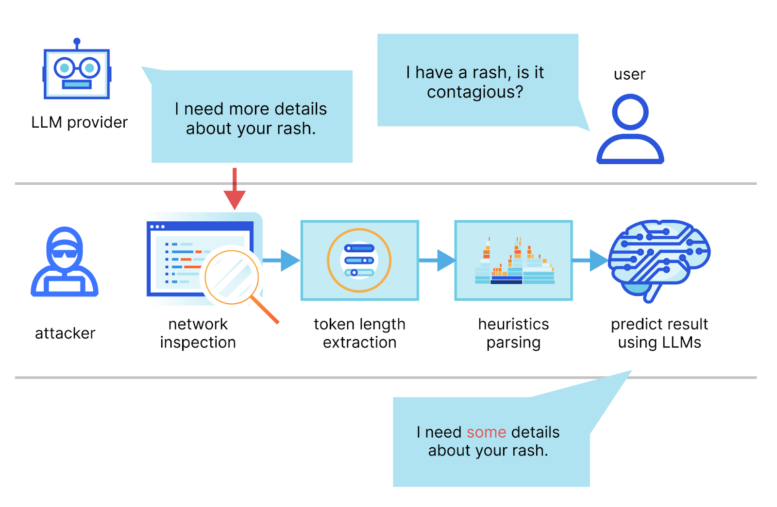
The two main requirements for a successful attack are an AI chat client running in streaming mode and a malicious actor capable of capturing network traffic between the client and the AI chat service. In streaming mode, the LLM tokens are emitted sequentially, introducing a token-length side-channel. Malicious actors could eavesdrop on packets via public networks or within an ISP.
An example request vulnerable to the side-channel attack looks like this:
curl -X POST \
https://api.cloudflare.com/client/v4/accounts/<account-id>/ai/run/@cf/meta/llama-2-7b-chat-int8 \
  -H "Authorization: Bearer <Token>" \
  -d '{"stream":true,"prompt":"tell me something about portugal"}'
Let’s use Wireshark to inspect the network packets on the LLM chat session while streaming:
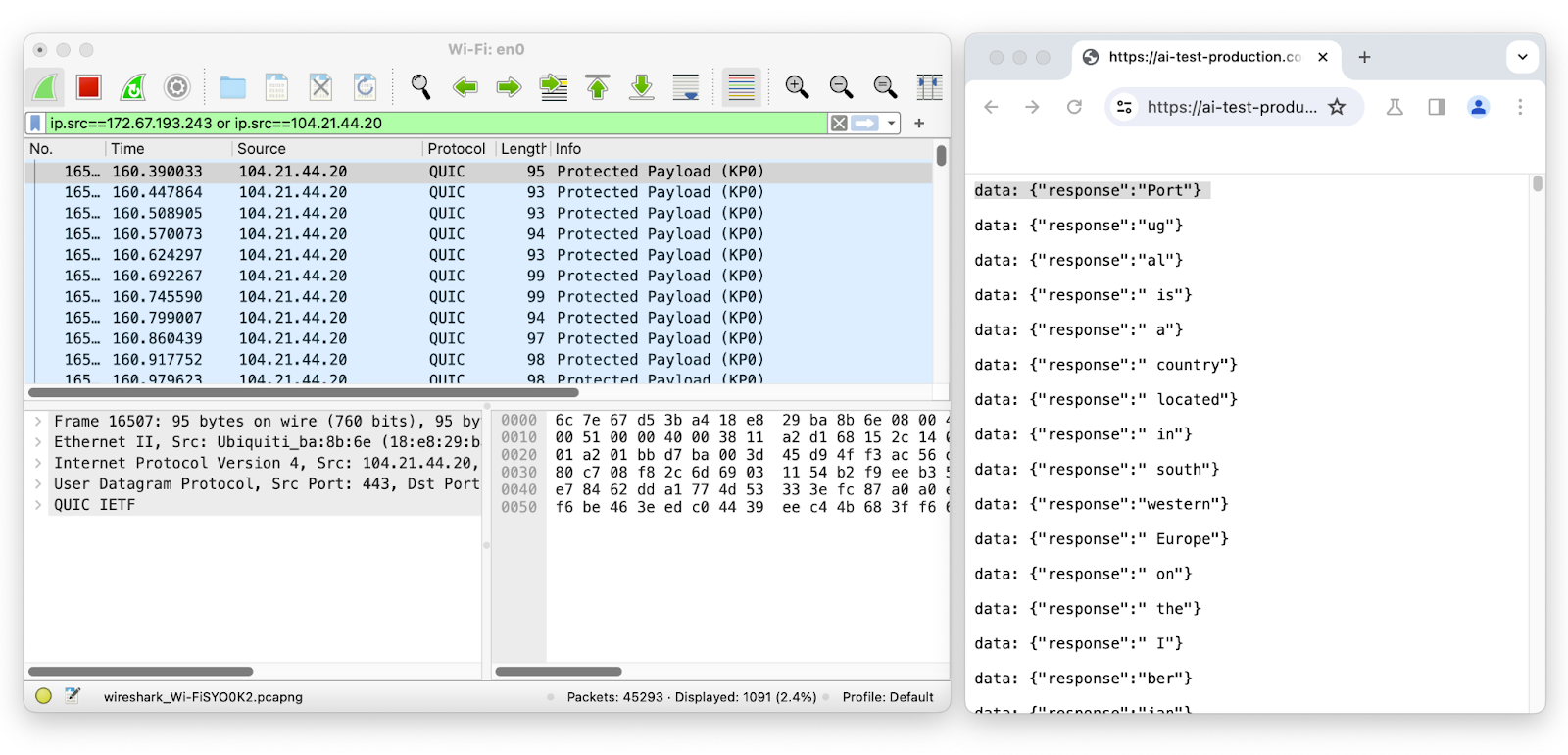
The first packet has a length of 95 and corresponds to the token “Port” which has a length of four. The second packet has a length of 93 and corresponds to the token “ug” which has a length of two, and so on. By removing the likely token envelope from the network packet length, it is easy to infer how many tokens were transmitted and their sequence and individual length just by sniffing encrypted network data.
Since the attacker needs the sequence of individual token length, this vulnerability only affects text generation models using streaming. This means that AI inference providers that use streaming — the most common way of interacting with LLMs — like Workers AI, are potentially vulnerable.
This method requires that the attacker is on the same network or in a position to observe the communication traffic and its accuracy depends on knowing the target LLM’s writing style. In ideal conditions, the researchers claim that their system “can reconstruct 29% of an AI assistant’s responses and successfully infer the topic from 55% of them”. It’s also important to note that unlike other side-channel attacks, in this case the attacker has no way of evaluating its prediction against the ground truth. That means that we are as likely to get a sentence with near perfect accuracy as we are to get one where only things that match are conjunctions.
Mitigating LLM side-channel attacks
Since this type of attack relies on the length of tokens being inferred from the packet, it can be just as easily mitigated by obscuring token size. The researchers suggested a few strategies to mitigate these side-channel attacks, one of which is the simplest: padding the token responses with random length noise to obscure the length of the token so that responses can not be inferred from the packets. While we immediately added the mitigation to our own inference product — Workers AI, we wanted to help customers secure their LLMs regardless of where they are running them by adding it to our AI Gateway.
As of today, all users of Workers AI and AI Gateway are now automatically protected from this side-channel attack.
What we did
Once we got word of this research work and how exploiting the technique could potentially impact our AI products, we did what we always do in situations like this: we assembled a team of systems engineers, security engineers, and product managers and started discussing risk mitigation strategies and next steps. We also had a call with the researchers, who kindly attended, presented their conclusions, and answered questions from our teams.
Unfortunately, at this point, this research does not include actual code that we can use to reproduce the claims or the effectiveness and accuracy of the described side-channel attack. However, we think that the paper has theoretical merit, that it provides enough detail and explanations, and that the risks are not negligible.
We decided to incorporate the first mitigation suggestion in the paper: including random padding to each message to hide the actual length of tokens in the stream, thereby complicating attempts to infer information based solely on network packet size.
Workers AI, our inference product, is now protected
With our inference-as-a-service product, anyone can use the Workers AI platform and make API calls to our supported AI models. This means that we oversee the inference requests being made to and from the models. As such, we have a responsibility to ensure that the service is secure and protected from potential vulnerabilities. We immediately rolled out a fix once we were notified of the research, and all Workers AI customers are now automatically protected from this side-channel attack. We have not seen any malicious attacks exploiting this vulnerability, other than the ethical testing from the researchers.
Our solution for Workers AI is a variation of the mitigation strategy suggested in the research document. Since we stream JSON objects rather than the raw tokens, instead of padding the tokens with whitespace characters, we added a new property, “p” (for padding) that has a string value of variable random length.
Example streaming response using the SSE syntax:
data: {"response":"portugal","p":"abcdefghijklmnopqrstuvwxyz0123456789a"}
data: {"response":" is","p":"abcdefghij"}
data: {"response":" a","p":"abcdefghijklmnopqrstuvwxyz012"}
data: {"response":" southern","p":"ab"}
data: {"response":" European","p":"abcdefgh"}
data: {"response":" country","p":"abcdefghijklmno"}
data: {"response":" located","p":"abcdefghijklmnopqrstuvwxyz012345678"}
This has the advantage that no modifications are required in the SDK or the client code, the changes are invisible to the end-users, and no action is required from our customers. By adding random variable length to the JSON objects, we introduce the same network-level variability, and the attacker essentially loses the required input signal. Customers can continue using Workers AI as usual while benefiting from this protection.
One step further: AI Gateway protects users of any inference provider
We added protection to our AI inference product, but we also have a product that proxies requests to any provider — AI Gateway. AI Gateway acts as a proxy between a user and supported inference providers, helping developers gain control, performance, and observability over their AI applications. In line with our mission to help build a better Internet, we wanted to quickly roll out a fix that can help all our customers using text generation AIs, regardless of which provider they use or if they have mitigations to prevent this attack. To do this, we implemented a similar solution that pads all streaming responses proxied through AI Gateway with random noise of variable length.
Our AI Gateway customers are now automatically protected against this side-channel attack, even if the upstream inference providers have not yet mitigated the vulnerability. If you are unsure if your inference provider has patched this vulnerability yet, use AI Gateway to proxy your requests and ensure that you are protected.
Conclusion
At Cloudflare, our mission is to help build a better Internet – that means that we care about all citizens of the Internet, regardless of what their tech stack looks like. We are proud to be able to improve the security of our AI products in a way that is transparent and requires no action from our customers.
We are grateful to the researchers who discovered this vulnerability and have been very collaborative in helping us understand the problem space. If you are a security researcher who is interested in helping us make our products more secure, check out our Bug Bounty program at hackerone.com/cloudflare.
Интервю на Георги Георгиев от БОЕЦ: „ДАНС е предала пътната карта за Турски поток на Стефан Янев, Кирил Петков не е знаел“
Post Syndicated from Николай Марченко original https://bivol.bg/boec-geoergiev-turskipotok.html
четвъртък 14 март 2024

Пътната карта за газопровода „Турски поток 2“ („Балкански поток“) е открита от Държавна агенция „Национална сигурност“ (ДАНС) още през 2021 г. Това сподели в интервю за „Биволъ“ председателят на гражданското…
Automakers Are Sharing Driver Data with Insurers without Consent
Post Syndicated from Bruce Schneier original https://www.schneier.com/blog/archives/2024/03/automakers-are-sharing-driver-data-with-insurers-without-consent.html
Kasmir Hill has the story:
Modern cars are internet-enabled, allowing access to services like navigation, roadside assistance and car apps that drivers can connect to their vehicles to locate them or unlock them remotely. In recent years, automakers, including G.M., Honda, Kia and Hyundai, have started offering optional features in their connected-car apps that rate people’s driving. Some drivers may not realize that, if they turn on these features, the car companies then give information about how they drive to data brokers like LexisNexis [who then sell it to insurance companies].
Automakers and data brokers that have partnered to collect detailed driving data from millions of Americans say they have drivers’ permission to do so. But the existence of these partnerships is nearly invisible to drivers, whose consent is obtained in fine print and murky privacy policies that few read.
State Medical Boards: Last Week Tonight with John Oliver (HBO)
Post Syndicated from LastWeekTonight original https://www.youtube.com/watch?v=jVIYbgVks7E
Digital forgeries are hard
Post Syndicated from Matthew Garrett original https://mjg59.dreamwidth.org/69507.html
Closing arguments in the trial between various people and Craig Wright over whether he’s Satoshi Nakamoto are wrapping up today, amongst a bewildering array of presented evidence. But one utterly astonishing aspect of this lawsuit is that expert witnesses for both sides agreed that much of the digital evidence provided by Craig Wright was unreliable in one way or another, generally including indications that it wasn’t produced at the point in time it claimed to be. And it’s fascinating reading through the subtle (and, in some cases, not so subtle) ways that that’s revealed.
One of the pieces of evidence entered is screenshots of data from Mind Your Own Business, a business management product that’s been around for some time. Craig Wright relied on screenshots of various entries from this product to support his claims around having controlled meaningful number of bitcoin before he was publicly linked to being Satoshi. If these were authentic then they’d be strong evidence linking him to the mining of coins before Bitcoin’s public availability. Unfortunately the screenshots themselves weren’t contemporary – the metadata shows them being created in 2020. This wouldn’t fundamentally be a problem (it’s entirely reasonable to create new screenshots of old material), as long as it’s possible to establish that the material shown in the screenshots was created at that point. Sadly, well.
One part of the disclosed information was an email that contained a zip file that contained a raw database in the format used by MYOB. Importing that into the tool allowed an audit record to be extracted – this record showed that the relevant entries had been added to the database in 2020, shortly before the screenshots were created. This was, obviously, not strong evidence that Craig had held Bitcoin in 2009. This evidence was reported, and was responded to with a couple of additional databases that had an audit trail that was consistent with the dates in the records in question. Well, partially. The audit record included session data, showing an administrator logging into the data base in 2011 and then, uh, logging out in 2023, which is rather more consistent with someone changing their system clock to 2011 to create an entry, and switching it back to present day before logging out. In addition, the audit log included fields that didn’t exist in versions of the product released before 2016, strongly suggesting that the entries dated 2009-2011 were created in software released after 2016. And even worse, the order of insertions into the database didn’t line up with calendar time – an entry dated before another entry may appear in the database afterwards, indicating that it was created later. But even more obvious? The database schema used for these old entries corresponded to a version of the software released in 2023.
This is all consistent with the idea that these records were created after the fact and backdated to 2009-2011, and that after this evidence was made available further evidence was created and backdated to obfuscate that. In an unusual turn of events, during the trial Craig Wright introduced further evidence in the form of a chain of emails to his former lawyers that indicated he had provided them with login details to his MYOB instance in 2019 – before the metadata associated with the screenshots. The implication isn’t entirely clear, but it suggests that either they had an opportunity to examine this data before the metadata suggests it was created, or that they faked the data? So, well, the obvious thing happened, and his former lawyers were asked whether they received these emails. The chain consisted of three emails, two of which they confirmed they’d received. And they received a third email in the chain, but it was different to the one entered in evidence. And, uh, weirdly, they’d received a copy of the email that was submitted – but they’d received it a few days earlier. In 2024.
And again, the forensic evidence is helpful here! It turns out that the email client used associates a timestamp with any attachments, which in this case included an image in the email footer – and the mysterious time travelling email had a timestamp in 2024, not 2019. This was created by the client, so was consistent with the email having been sent in 2024, not being sent in 2019 and somehow getting stuck somewhere before delivery. The date header indicates 2019, as do encoded timestamps in the MIME headers – consistent with the mail being sent by a computer with the clock set to 2019.
But there’s a very weird difference between the copy of the email that was submitted in evidence and the copy that was located afterwards! The first included a header inserted by gmail that included a 2019 timestamp, while the latter had a 2024 timestamp. Is there a way to determine which of these could be the truth? It turns out there is! The format of that header changed in 2022, and the version in the email is the new version. The version with the 2019 timestamp is anachronistic – the format simply doesn’t match the header that gmail would have introduced in 2019, suggesting that an email sent in 2022 or later was modified to include a timestamp of 2019.
This is by no means the only indication that Craig Wright’s evidence may be misleading (there’s the whole argument that the Bitcoin white paper was written in LaTeX when general consensus is that it’s written in OpenOffice, given that’s what the metadata claims), but it’s a lovely example of a more general issue.
Our technology chains are complicated. So many moving parts end up influencing the content of the data we generate, and those parts develop over time. It’s fantastically difficult to generate an artifact now that precisely corresponds to how it would look in the past, even if we go to the effort of installing an old OS on an old PC and setting the clock appropriately (are you sure you’re going to be able to mimic an entirely period appropriate patch level?). Even the version of the font you use in a document may indicate it’s anachronistic. I’m pretty good at computers and I no longer have any belief I could fake an old document.
(References: this Dropbox, under “Expert reports”, “Patrick Madden”. Initial MYOB data is in “Appendix PM7”, further analysis is in “Appendix PM42”, email analysis is “Sixth Expert Report of Mr Patrick Madden”)
![]() comments
comments
Преди изборите, или как се става кандидат-президент в САЩ
Post Syndicated from Йоанна Елми original https://www.toest.bg/predi-izborite-ili-kak-se-stava-kandidat-prezident-v-usa/
Изборите в САЩ, част I. Механизмите на вота

Независимо дали обикаляте по улиците на Вашингтон, окръг Колумбия, или се разхождате из малки курортни градчета като Оушън Сити в Мериленд, може да си купите тениска както с лика на Джо Байдън, така и на Доналд Тръмп – и то от един и същи продавач. Излитащите от „Джон Ф. Кенеди“ в Ню Йорк пък могат да занесат у дома сувенирни шоколади с лика на 45-тия или 46-тия американски президент. Под това прозира не само търговска находчивост, американската способност всичко да се превръща в продукт или поредната изборна година, а и дълбоките разделения, които едновременно уж разкъсват обществената тъкан в Америка, но и са всекидневие, към което всички са привикнали.
САЩ е ключов партньор на България, световна сила и основна страна във все по-горещ военен конфликт, така че предстоящите през ноември президентски избори разбираемо вълнуват не само българите, но и света. Същевременно от САЩ ни дели цял океан, а дигиталната близост до американския свят е илюзорна: за много европейци например изборният процес в Америка е тъмна материя. У нас американската политика често се разглежда или през кратки новини и очерци, или през превратното тълкуване на източници на дезинформация – като тези, които по-рано през годината обявиха началото на гражданска война в САЩ, която така и не се състоя.
Но това, че Америка е любима тема на антидемократичната пропаганда в България, не означава, че отвъд океана няма съвсем реални и сериозни проблеми. Тяхното разбиране е свързано не само с интереса ни към политиката. То може да ни помогне да разберем по-добре как работи демокрацията, а също и какво може да се случи, когато механизмите ръждясат и не се сменят с нови. Затова в поредица от статии ще разгледаме някои от най-често задаваните въпроси, свързани с американските избори, и ще разнищим защо всъщност е толкова трудно да си направиш демокрация. Започваме от самото начало.
Първичните избори
Американските избори са сложен процес с повече стъпки, отколкото стандартните европейски избори. Кампаниите често започват в предходната година, като има множество кандидати от всяка партия. Традиция е партията на управляващия президент да не излъчва други кандидати, ако той е отслужил само един мандат, тоест ако има право на още един. Затова и настоящият президент Джо Байдън не бе предизвикан от свой съпартиец. От 70-те години насам няма действащ президент, който да е бил победен по този начин по време на предварителните избори.
Тази година обаче в някои щати рекорден брой избиратели на демократите избраха варианта „не подкрепям никого“ по време на първичните избори. Това е резултат от гражданска акция, която използва протестен вот като наказание за политиката на САЩ в конфликта между Израел и Палестина. След терористичната атака на „Хамас“ на 7 октомври 2023 г. и последвалия отговор на Израел (подкрепян от САЩ), към момента са убити над 30 000 цивилни палестинци. Палестинските територии са в хуманитарна криза, като се трупат все повече доказателства за диспропорционално използване на сила от страна на Израел спрямо цивилното население. Конфликтът в Близкия изток подхранва разделения в Демократическата партия и може да предизвика отлив в подкрепата за настоящия президент.
В изборна година всяко едно събитие, независимо дали става въпрос за вътрешен, или външен конфликт, може да наклони везните в една или друга посока. Същевременно обаче в САЩ се наблюдава т.нар. втвърдяване на електората, за което ще разкажем подробно в следващите текстове. Този феномен води до твърди електорални ядра, които подкрепят кандидатите си независимо от всичко – дори да става дума за множество престъпления като при кандидата на републиканците Доналд Тръмп, за някои от които той вече е осъден.
Какво представлява Избирателната колегия и демократична ли е тя?
През 2016 г. Доналд Тръмп спечели изборите, въпреки че по-голяма част от американците гласуваха за Хилари Клинтън. Как се случи това и възможно ли е през 2024 г. да има повторение?
Демокрацията в САЩ не е пряка, както в много европейски държави. В преките демокрации бюлетините се броят и общият брой се преизчислява в проценти подкрепа за всяка партия. Но когато американците гласуват, те всъщност избират кого ще изберат определени хора от техния щат.
Звучи сложно? Вероятно защото е. Тези определени хора са част от Избирателната колегия, разписана в американската Конституция от основателите като компромис между директното избиране на президента с гласуване и неговото назначаване от Конгреса. Именно заради Избирателната колегия пет пъти в историята на САЩ се е случвало президент, който не е спечелил най-много гласове, всъщност да спечели изборите.
Колегията има 538 членове. Президентът е избран, ако получи поне 270 от тези 538 гласа. Основният аргумент в полза на Избирателната колегия е, че делегирани представители биха могли да вземат по-добро решение от масите, избягвайки потенциална тирания на мнозинството над малцинството или подвеждане по популисти и демагози.
Разбира се, нищо не гарантира, че членовете на Избирателната колегия са по-образовани или по-компетентни от средностатистическия избирател – днес те са просто партийни назначения, които законите в някои щати задължават да се съобразят с волята на избирателите. На изборите през 2016 г. рекорден брой електори не го направиха. Някои от електорите на демократите например гласуваха за Бърни Сандърс вместо за Хилари Клинтън, тъй като предварителните избори бяха разцепили поддръжниците на партията на две крила.
Защитниците на Избирателната колегия твърдят, че така се осигурява пропорционално представителство на цялото население на Щатите. В противен случай кандидатите биха концентрирали усилията си върху големите населени места, където има най-много гласоподаватели, и напълно биха игнорирали нуждите на централните, по-слабо населени щати.
Но в съвремието нуждите и интересите на гласоподавателите не се определят от населението или от големината на техния щат. Разделенията по основните въпроси, като климатичните промени, правото на аборт или Втората поправка, са актуални както в градовете, така и в малките населени места, като в повечето щати има сравнително разнообразие от привърженици на републиканците и демократите, както и безпартийни гласоподаватели.
Все повече експерти са категорични, че Избирателната колегия е недемократична и следва да бъде премахната. Този процес никога не е бил особено популярен и сред гласоподавателите: данни от есента на 2023 г. показват, че 65% от американците искат пряко гласуване на президентски избори. Вместо да има изравняващ ефект между щатите, Избирателната колегия създава т.нар. колебаещи се щати. Те се променят през годините, но идеята е, че получават непропорционално внимание от кандидатите, които са наясно, че гласовете на електорите в останалите щати са им гарантирани. Това оборва и най-силния аргумент в полза на Избирателната колегия.
Тъй като обаче Колегията обикновено се защитава от онези, в чиято полза работи, Републиканската партия от години блокира нейното премахване, за което призовават демократите. Това е поредна разломна линия между двете партии, превърнала се в заложник по-скоро на политически интереси, отколкото на вслушване в желанието на мнозинството.


Какво представляват партийните комитети и какво е Супервторник?
В САЩ съществуват и т.нар. партийни комитети – различни групи, съставени от членове на съответната партия. Тяхната роля да номинират кандидати е ключова в първичните избори, завършващ с т.нар. Супервторник (тази година той беше в началото на март). След Супервторника – последния ден, в който членовете на дадена партия в определен щат гласуват за предпочитаната от тях номинация, е ясен кандидатът за президент от всяка партия, който ще се яви на същинските избори.
Партийните комитети се появяват през 1800 г. и са съставени от членове на Конгреса, които номинират кандидат-президенти. Критиките към тях са, че не успяват да гарантират разделението на властите, т.е. принципа, според който трите власти – изпълнителна (президент), законодателна (Конгрес и Камара на представителите) и съдебна (Върховен съд и съдилища) – трябва да бъдат независими една от друга. През 1812 г. например върху президента Джеймс Мадисън е оказван натиск от членове на Конгреса, които поставят условие той да обяви война на Обединеното кралство, ако иска да го номинират повторно.
Напрежението, породено от тази система, достига своя пик през 1824 г., когато нито един от кандидатите, номинирани от партийните комитети, не успява да спечели достатъчно гласове и де факто Конгресът трябва да назначи президент. Тогавашната криза и назначението на по-малко популярния кандидат води до разпадането на първата двупартийна система в САЩ и появата на настоящите две партии, макар и не във вида, в който ги познаваме днес.
Партийните комитети остават силно недемократични до 60-те години на миналия век. На предварителните избори дотогава се гледа по-скоро като на тест дали кандидатът, избран от една партия, ще се справи добре на същинските избори. От 1968 г. насам Демократическата партия постоянно променя функционирането на своите партийни комитети, опитвайки се все повече да ги демократизира. Това е дълъг (и със сигурност скучен за читателя) процес на нововъведения, отмяна на нововъведенията и замяната им с други, разписване на забраненото и позволеното в процеса и т.н. Подобна е ситуацията и при републиканците, които дават повече свобода на щатите сами да определят правила за партийните си комитети.
Какво ни показват тези сложни механизми?
Ако от всичко това ви е заболяла глава, не сте единствени. Освен класическото разделение на властите, цялата система на управление на САЩ е изградена от подобни микропроверки и баланси, които понякога работят, а понякога отнемат повече свободи, отколкото дават, в добрите случаи – временно. Компромисът за Избирателната колегия е само един от многото, заложени още в основите на държавата. Тези компромиси между често взаимно изключващи се позиции осигуряват така необходимия баланс, в който може да вирее някаква свобода, включително и най-важната – да се променят вече установени механизми.
Илюзорно разбиране е, че демокрацията гарантира пълна ефективност на управлението или някаква утопия. Напротив, демокрацията е по-хаотична, изисква повече време и често предполага натиск и борба между определени групи, за да се стигне до най-доброто решение за всички. Демокрацията също така не е равнозначна на свобода и равенство, а само на равния шанс да се стремим към тях и на държава, която ни пази ефективно както от самата себе си, така и от самите нас.
На север: Страната на инуитите
Post Syndicated from Светла Стоянова original https://www.toest.bg/stranata-na-inuitite/

<< Към На север: Гренландия и тайните на леда
Събудих се през нощта и слънцето грееше, като че беше ярък следобед. Зачудих се как ли човек не полудява тук – от постоянната светлина или от постоянната тъмнина през останалата част от годината. Как ли гренландците успяват да живеят на това толкова особено място на планетата?
Инуитите населяват най-отдалечените и най-северни райони в света и вероятно са един от най-добре приспособените етноси към арктическия климат и условия. Чрез специфичните си умения и начин на живот те са се научили да оцеляват при температури до –40°С.
Названието ескимоси, с което са по-познати у нас, вероятно води началото си от друг етнос в Северна Америка, който наричал инуитите „онези, които ядат сурово месо“. Негативната конотация в наименованието се запазва през вековете, като се създава цялостен принизяващ стереотип за етноса. Местното население на Гренландия говори за себе си като
инуити, което в превод означава „хòра“.
В миналото земите на Гренландия са населявани и от други етноси. Най-ранният е саккак, отпреди повече от 2500 г.пр.Хр., след него идва дорсет, около 400 г.пр.Хр., а след това и туле, чиито потомци са днешните инуити, преселили се от Канада по замръзналата повърхност на океана през Малкия ледников период на Средновековието. През Х в. до Гренландия с кораби достигат и викингите. Те се задържат там няколко века, докато не изчезват – може би заради критичното застудяване на климата.
През XVIII в. датско-норвежкият мисионер Ханс Егеде е изпратен в Гренландия, за да открие викингите и да ги покръсти. Той тръгва със семейството си и още няколко кораба и заживява в днешен Нуук, наречен от него Готхоб, в превод – „Добра надежда“. Ханс Егеде не намира викинги, но прави усилия да покръсти местното население.

Съвсем естествено, Егеде среща известни трудности в междуезиковото разбиране при проповядването на християнството. Забавен пример за това е преводът на изречението „Дай ни насъщния хляб!“. Хлябът в Гренландия е също толкова непознат, колкото за Европа са били непознати гренландците по онова време, и е било трудно да се разбере за какво става дума. Егеде смята, че е открил подходящо съответствие на символичната сила на думата хляб в речта им, защото, докато се хранят, местните често произнасят маммак и сочат храната. Затова той променя молитвата така: „Дай ни насъщния маммак!“. Впоследствие обаче, след поредните озадачаващи реакции, установява, че маммак е просто възклицание – „Колко вкусно!“. По-късно решава да използва думата за тюленско месо, тъй като именно то е също толкова често на масата, колкото хлябът в Европа.
Гренландският език е част от ескимо-алеутското езиково семейство. Той е полисинтетичен, тоест едно изречение често се слива в една много дълга дума. Най-ранните структурирани писмени сведения за езика са в първата гренландска граматика, написана от Пол Егеде, сина на мисионера Ханс Егеде, който, за разлика от баща си, научава гренландски добре и умее да общува с местните.

Живеейки в Гренландия, за мен също беше важно да общувам с местните. Исках да науча повече за тях, за начина им на живот и за светогледа им. Вероятно и заради това такава беше една от първите ми срещи с тях:
Вървях по улицата по края на града и насреща ми мина една малка червена кола с гренландец, който ми се усмихна. Само след малко колата мина отново в моята посока и спря. Реших, че човекът може би предлага да ме закара до града, и се качих. Питах го дали има книжарница наблизо, но той не ме разбра. Разговаряхме на смесица между неговия развален английски и датски с гренландски акцент и моя датски с норвежко произношение. Усмихнат и доволен, явно беше решил да ме разведе в града. Питах го има ли семейство, и отговорът беше: да – само баща и брат. Мина ми през ума, че може би е било твърде смело да се качвам просто така в колата му, но обясних къде работя, и вярвах, че всичко ще бъде наред. Той обиколи града, като спираше на места, показвайки гордо двете си лодки, къщата си, а най-накрая шейната и кучетата си, на които явно много държеше – цели трийсет, от които двайсет бяха още кутрета. Докато вървяхме към тях през тревата и калта, той предложи ръката си, но аз само поклатих глава с усмивка. Това като че го смути, но се засмя. Когато нахрани кучетата, му направих знак, че все пак трябва да тръгвам. Разбра ме и с неохота ме закара. Беше ми показал най-ценното си – къщата, лодките, колата, шейната и кучетата.
Интересен е животът на инуитите, които са съумели толкова добре да се приспособят към екстремните условия на живот в Арктика. По техните земи няма нито плодове, нито зеленчуци и единствените източници на храна са дивите животни – северни елени, тюлени, моржове, китове, птици и риби. В миналото хората са използвали специални харпуни за лов на тюлени, а китовете хващали с по-големи лодки, наречени умиак. През лятото семействата осигурявали прехраната си с лъкове и стрели и живеели в юрти, покрити с кожи от заловените животни. Зимували в обли къщи, направени от блокове сняг, познати като иглу, или в полуподземни къщи, построени от камъни и кожи върху пòкривна конструкция от трупи или кости от кит. В днешно време харпуните и лъковете се заменят с пушки, а юртите и иглуто – с дървени къщи.
За улова на всички животни е определена квота, като например ограничението за лов на китове е два броя годишно за целия остров.
Когато бях на гости у едно семейство инуити, стопанинът гордо показа огромния си фризер, с който явно всеки уважаващ себе си гренландец разполага и който беше пълен с полуразфасовано месо от най-различни животни. Жената пък извади големи пликове със замразени боровинки, които беше събирала през лятото. Различните видове боровинки са единствените плодове, растящи на острова.
Друго типично за ежедневието на инуитите са шейните с кучешки впрягове. Те са основният начин на придвижване през зимата, което предполага, че глутницата трябва да бъде хранена целогодишно. Шейните с кучешки впряг обикновено са гордост за семейството. Мъжете ги правят по свой размер и участват в ежегодни надбягвания. Един познат гренландец ми разказа, че мечтае да има свой кучешки впряг, но разрастването и обучението на глутницата отнемало години. Част от младите инуити като него през лятото работят като екскурзоводи, а през зимата – във фабрики за риба. Желанието му беше вместо това да заработва в бъдеще като гид с кучешкия си впряг. Притежанието на кучета също така означавало и по-висок статус в обществото. В днешно време обаче все повече гренландци ги заменят със снегомобили – все пак тях не е нужно да ги хранят с риба и еленско месо през цялата година.

Друга инуитска традиция е карането на каяк. Традиционно той се прави от дълги и тънки дъски и тюленски кожи. Благодарение на изключителната си лекота и маневреност е идеален за лов на тюлени. Заради тези качества каякът бързо се разпространява сред полярните изследователи, които неведнъж посещават инуитските племена и черпят знания и опит от техните изключителни методи за оцеляване. Малко известен факт е, че думата каяк, използвана в повечето европейски езици, е именно инуитска. Веднъж дори станах свидетелка на ежегодното първенство по каяк в Гренландия, което включваше дисциплини по бързина, издръжливост и специални умения, като впечатляващото преобръщане на 360 градуса с каяка във водата. Освен това беше задължително каяците да са измайсторени от самите състезатели.

Инуитите държат на традициите, но обществото все повече се модернизира с развитието на инфраструктурата и туризма. Има много работни места в предприятия за риба и скариди благодарение на големия износ в последните години. Съвременното гренландско общество е пръснато по градове и села. Връзки между градовете няма, освен по море, по лед или по въздух. Тоест пътища между селищата не съществуват, а коли може да се видят само в най-големите градове. За извънградско пътуване се използват най-вече лодки или фериботи. Един мой познат разказваше как всяко лято нямал търпение да потегли отново на 18-часовото си плаване с моторната си лодка на юг по западното крайбрежие, за да посети своите роднини.
В селото на име Илиманак, в което прекарах няколко месеца, живеят петдесетина гренландци. Пристигайки, човек се изкачва по стръмен кей, около който се клатушкат навързани множество лодки. Досами кея се вижда магазин и в него се продава всичко – от мляко и ябълки до въдици и пушки. За няколкото деца в селото е учредено училище с местна учителка. Съвсем наблизо е и селската баня, служеща едновременно за перално помещение, фитнес зала и кафене. Банята работи с купони за душа, които служител перфорира преди всяко къпане. Често същата сграда, изпълняваща множество функции, се превръща в място за спонтанни срещи.


Къщи в Илиманак © Светла Стоянова
Характерна черта за гренландските къщи е, че са боядисани в ярки и весели цветове – червено, розово, синьо, тюркоазено, жълто.
Някои от тях са окичени с ловни трофеи, като еленски рога, или с козината на бели мечки. Пътеките между къщите са частично циментирани, а наоколо занемарени стоят недовършени проекти и неизхвърлени боклуци. Често недалеч от домовете стопаните връзват кучетата си.
В повечето селища от подобен тип няма канализация, защото няма достатъчно средства за инфраструктурата. Водата се извежда по тръба от близкото езеро, минава през моторна помпа и стига по дълъг маркуч до резервоара на всяка къща, после от кухненската чешма изтича от умивалника директно навън, където образува голяма локва. А ако има тръби, те рано или късно извеждат отпадните води направо в океана. Тоалетната чиния прилича на нормална, но в нея се поставят огромни черни пликове, които трябва да се сменят редовно. Използваните пликове, затегнати с тел, се поставят на определено видно място до къщата, така че отговорникът за това да ги вижда и да ги събира своевременно.
Един мой приятел гренландец ми каза, че истинската Гренландия е именно тази, на север от Полярния кръг, точно тук, в малките селища. Защото, който иска да я изживее, трябва да прекара известно време в дивото и извън удобствата, с които толкова сме свикнали.
(Следва продължение.)
Introducing Sunlight, a CT implementation built for scalability, ease of operation, and reduced cost
Post Syndicated from Let's Encrypt original https://letsencrypt.org/2024/03/14/introducing-sunlight/
Let’s Encrypt is proud to introduce Sunlight, a new implementation of a Certificate Transparency log that we built from the ground up with modern Web PKI opportunities and constraints in mind. In partnership with Filippo Valsorda, who led the design and implementation, we incorporated feedback from the broader transparency logging community, including the Chrome and TrustFabric teams at Google, the Sigsum project, and other CT log and monitor operators. Their insights have been instrumental in shaping the project’s direction.
CT plays an important role in the Web PKI, enhancing the ability to monitor and research certificate issuance. The operation of a CT log, however, faces growing challenges with the increasing volume of certificates. For instance, Let’s Encrypt issues over four million certificates daily, each of which must be logged in two separate CT logs. Our well-established “Oak” log currently holds over 700 million entries, reflecting the significant scale of these challenges.
In this post, we’ll explore the motivation behind Sunlight and how its design aims to improve the robustness and diversity of the CT ecosystem, while also improving the reliability and performance of Let’s Encrypt’s logs.
Bottlenecks from the Database
Let’s Encrypt has been running public CT logs since 2019, and we’ve gotten a lot of operational experience with running them, but it hasn’t been trouble-free. The biggest challenge in the architecture we’ve deployed for our “Oak” log is that the data is stored in a relational database. We’ve scaled that up by splitting each year’s worth of data into a “shard” with its own database, and then later shrinking the shards to cover six months instead of a full year.
The approach of splitting into more and more databases is not something we want to continue doing forever, as the operational burden and costs increase. The current storage size of a CT log shard is between 5 and 10 terabytes. That’s big enough to be concerning for a single database: We previously had a test log fail when we ran into a 16TiB limit in MySQL.
Scaling read capacity up requires large database instances with fast disks and lots of RAM, which are not cheap. We’ve had numerous instances of CT logs becoming overloaded by clients attempting to read all the data in the log, overloading the database in the process. When rate limits are imposed to prevent overloading, clients are forced to slowly crawl the API, diminishing CT’s efficiency as a fast mechanism for detecting mis-issued certificates.
Serving Tiles
Initially, Let’s Encrypt only planned on building a new CT log implementation. However, our discussions with Filippo made us realize that other transparency systems had improved on the original Certificate Transparency design, and we could make our logs even more robust and scalable by changing the read path APIs. In particular, the Go Checksum Database is inspired by Certificate Transparency, but uses a more efficient format for publishing its data as a series of easily stored and cached tiles.
Certificate Transparency logs are a binary tree, with every node containing a hash of its two children. The “leaf” level contains the actual entries of the log: the certificates, appended to the right side of the tree. The top of the tree is digitally signed. This forms a cryptographically verifiable structure called a Merkle Tree, which can be used to check if a certificate is in the tree, and that the tree is append-only.
Sunlight tiles are files containing 256 elements each, either hashes at a certain tree “height” or certificates (or pre-certificates) at the leaf level. Russ Cox has a great explanation of how tiles work on his blog, or you can read the relevant section of the Sunlight specification. Even Trillian, the current implementation of CT we run, uses a subtree system similar to these tiles as its internal storage.
Unlike the dynamic endpoints in previous CT APIs, serving a tree as tiles doesn’t require any dynamic computation or request processing, so we can eliminate the need for API servers. Because the tiles are static, they’re efficiently cached, in contrast with CT APIs like get-proof-by-hash which have a different response for every certificate, so there’s no shared cache. The leaf tiles can also be stored compressed, saving even more storage!
The idea of exposing the log as a series of static tiles is motivated by our desire to scale out the read path horizontally and relatively inexpensively. We can directly expose tiles in cloud object storage like S3, use a caching CDN, or use a webserver and a filesystem.
Object or file storage is readily available, can scale up easily, and costs significantly less than databases from cloud providers. It seemed like the obvious path forward. In fact, we already have an S3-backed cache in front of our existing CT logs, which means we are currently storing our data twice.
Running More Logs
The tiles API improves the read path, but we also wanted to simplify our architecture on the write path. With Trillian, we run a collection of nodes along with etcd for leader election to choose which will handle writing. This is somewhat complex, and we believe the CT ecosystem allows a different tradeoff.
The key realization is that Certificate Transparency is already a distributed system, with clients submitting certificates to multiple logs, and gracefully failing over from any unavailable ones to the others. Each individual log’s write path doesn’t require a highly available leader election system. A simple single-node writer can meet the 99% Service Level Objective required by CT log programs.
The single-node Sunlight architecture lets us run multiple independent logs with the same amount of computing power. This increases the system’s overall robustness, even if each individual log has lower potential uptime. No more leader election needed. We use a simple compare-and-swap mechanism to store checkpoints and prevent accidentally running two instances at once, which could result in a forked tree, but that has much less overhead than leader election.
No More Merge Delay
One of the goals of CT was to have limited latency for submission to the logs. A design feature called Merge Delay was added to support that. When submitting a certificate to a log, the log can return a Signed Certificate Timestamp (SCT) immediately, with a promise to include it in the log within the log’s Maximum Merge Delay, conventionally 24 hours. While this seems like a good tradeoff to not slow down issuance, there have been multiple incidents and near-misses where a log stops operating with unmerged certificates, missing its maximum merge delay, and breaking that promise.
Sunlight takes a different approach, holding submissions while it batches and integrates certificates in the log, eliminating the merge delay. While this leads to a small latency increase, we think it’s worthwhile to avoid one of the more common CT log failure cases.
It also lets us embed the final leaf index in an extension of our SCTs, bringing CT a step closer to direct client verification of Merkle tree proofs. The extension also makes it possible for clients to fetch the proof of log inclusion from the new static tile-based APIs, without requiring server-side lookup tables or databases.
A Sunny Future
Today’s announcement of Sunlight is just the beginning. We’ve released software and a specification for Sunlight, and have Sunlight CT logs running. Head to sunlight.dev to find resources to get started. We encourage CAs to start test submitting to Let’s Encrypt’s new Sunlight CT logs, for CT Monitors and Auditors to add support for consuming Sunlight logs, and for the CT programs to consider trusting logs running on this new architecture. We hope Sunlight logs will be made usable for SCTs by the CT programs run by the browsers in the future, allowing CAs to rely on them to meet the browser CT logging requirements.
We’ve gotten positive feedback so far, with comments such as “Google’s TrustFabric team, maintainers of Trillian, are supportive of this direction and the Sunlight spec. We have been working towards the same goal of cacheable tile-based logs for other ecosystems with serverless tooling, and will be folding this into Trillian and ctfe, along with adding support for the Sunlight API.”
If you have feedback on the design, please join in the conversation on the ct-policy mailing list, or in the #sunlight channel on the transparency-dev Slack (invitation to join).
We’d like to thank Chrome for supporting the development of Sunlight, and Amazon Web Services for their ongoing support for our CT log operation. If your organization monitors or values CT, please consider a financial gift of support. Learn more at https://www.abetterinternet.org/sponsor/ or contact us at: [email protected].