Post Syndicated from The Atlantic original https://www.youtube.com/watch?v=_-qxXlHDDB0
[$] LWN.net Weekly Edition for September 28, 2023
Post Syndicated from corbet original https://lwn.net/Articles/945211/
The LWN.net Weekly Edition for September 28, 2023 is available.
Amazon MSK Introduces Managed Data Delivery from Apache Kafka to Your Data Lake
Post Syndicated from Sébastien Stormacq original https://aws.amazon.com/blogs/aws/amazon-msk-introduces-managed-data-delivery-from-apache-kafka-to-your-data-lake/
I’m excited to announce today a new capability of Amazon Managed Streaming for Apache Kafka (Amazon MSK) that allows you to continuously load data from an Apache Kafka cluster to Amazon Simple Storage Service (Amazon S3). We use Amazon Kinesis Data Firehose—an extract, transform, and load (ETL) service—to read data from a Kafka topic, transform the records, and write them to an Amazon S3 destination. Kinesis Data Firehose is entirely managed and you can configure it with just a few clicks in the console. No code or infrastructure is needed.
Kafka is commonly used for building real-time data pipelines that reliably move massive amounts of data between systems or applications. It provides a highly scalable and fault-tolerant publish-subscribe messaging system. Many AWS customers have adopted Kafka to capture streaming data such as click-stream events, transactions, IoT events, and application and machine logs, and have applications that perform real-time analytics, run continuous transformations, and distribute this data to data lakes and databases in real time.
However, deploying Kafka clusters is not without challenges.
The first challenge is to deploy, configure, and maintain the Kafka cluster itself. This is why we released Amazon MSK in May 2019. MSK reduces the work needed to set up, scale, and manage Apache Kafka in production. We take care of the infrastructure, freeing you to focus on your data and applications. The second challenge is to write, deploy, and manage application code that consumes data from Kafka. It typically requires coding connectors using the Kafka Connect framework and then deploying, managing, and maintaining a scalable infrastructure to run the connectors. In addition to the infrastructure, you also must code the data transformation and compression logic, manage the eventual errors, and code the retry logic to ensure no data is lost during the transfer out of Kafka.
Today, we announce the availability of a fully managed solution to deliver data from Amazon MSK to Amazon S3 using Amazon Kinesis Data Firehose. The solution is serverless–there is no server infrastructure to manage–and requires no code. The data transformation and error-handling logic can be configured with a few clicks in the console.
The architecture of the solution is illustrated by the following diagram.

Amazon MSK is the data source, and Amazon S3 is the data destination while Amazon Kinesis Data Firehose manages the data transfer logic.
When using this new capability, you no longer need to develop code to read your data from Amazon MSK, transform it, and write the resulting records to Amazon S3. Kinesis Data Firehose manages the reading, the transformation and compression, and the write operations to Amazon S3. It also handles the error and retry logic in case something goes wrong. The system delivers the records that can not be processed to the S3 bucket of your choice for manual inspection. The system also manages the infrastructure required to handle the data stream. It will scale out and scale in automatically to adjust to the volume of data to transfer. There are no provisioning or maintenance operations required on your side.
Kinesis Data Firehose delivery streams support both public and private Amazon MSK provisioned or serverless clusters. It also supports cross-account connections to read from an MSK cluster and to write to S3 buckets in different AWS accounts. The Data Firehose delivery stream reads data from your MSK cluster, buffers the data for a configurable threshold size and time, and then writes the buffered data to Amazon S3 as a single file. MSK and Data Firehose must be in the same AWS Region, but Data Firehose can deliver data to Amazon S3 buckets in other Regions.
Kinesis Data Firehose delivery streams can also convert data types. It has built-in transformations to support JSON to Apache Parquet and Apache ORC formats. These are columnar data formats that save space and enable faster queries on Amazon S3. For non-JSON data, you can use AWS Lambda to transform input formats such as CSV, XML, or structured text into JSON before converting the data to Apache Parquet/ORC. Additionally, you can specify data compression formats from Data Firehose, such as GZIP, ZIP, and SNAPPY, before delivering the data to Amazon S3, or you can deliver the data to Amazon S3 in its raw form.
Let’s See How It Works
To get started, I use an AWS account where there’s an Amazon MSK cluster already configured and some applications streaming data to it. To get started and to create your first Amazon MSK cluster, I encourage you to read the tutorial.
For this demo, I use the console to create and configure the data delivery stream. Alternatively, I can use the AWS Command Line Interface (AWS CLI), AWS SDKs, AWS CloudFormation, or Terraform.
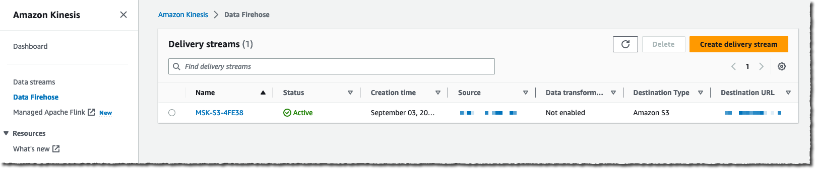
I navigate to the Amazon Kinesis Data Firehose page of the AWS Management Console and then choose Create delivery stream.
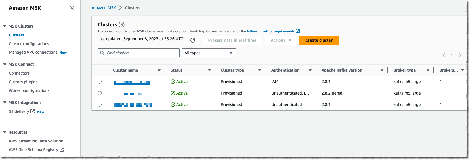
I select Amazon MSK as a data Source and Amazon S3 as a delivery Destination. For this demo, I want to connect to a private cluster, so I select Private bootstrap brokers under Amazon MSK cluster connectivity.
I need to enter the full ARN of my cluster. Like most people, I cannot remember the ARN, so I choose Browse and select my cluster from the list.
Finally, I enter the cluster Topic name I want this delivery stream to read from.

After the source is configured, I scroll down the page to configure the data transformation section.
On the Transform and convert records section, I can choose whether I want to provide my own Lambda function to transform records that aren’t in JSON or to transform my source JSON records to one of the two available pre-built destination data formats: Apache Parquet or Apache ORC.
Apache Parquet and ORC formats are more efficient than JSON format to query data from Amazon S3. You can select these destination data formats when your source records are in JSON format. You must also provide a data schema from a table in AWS Glue.
These built-in transformations optimize your Amazon S3 cost and reduce time-to-insights when downstream analytics queries are performed with Amazon Athena, Amazon Redshift Spectrum, or other systems.

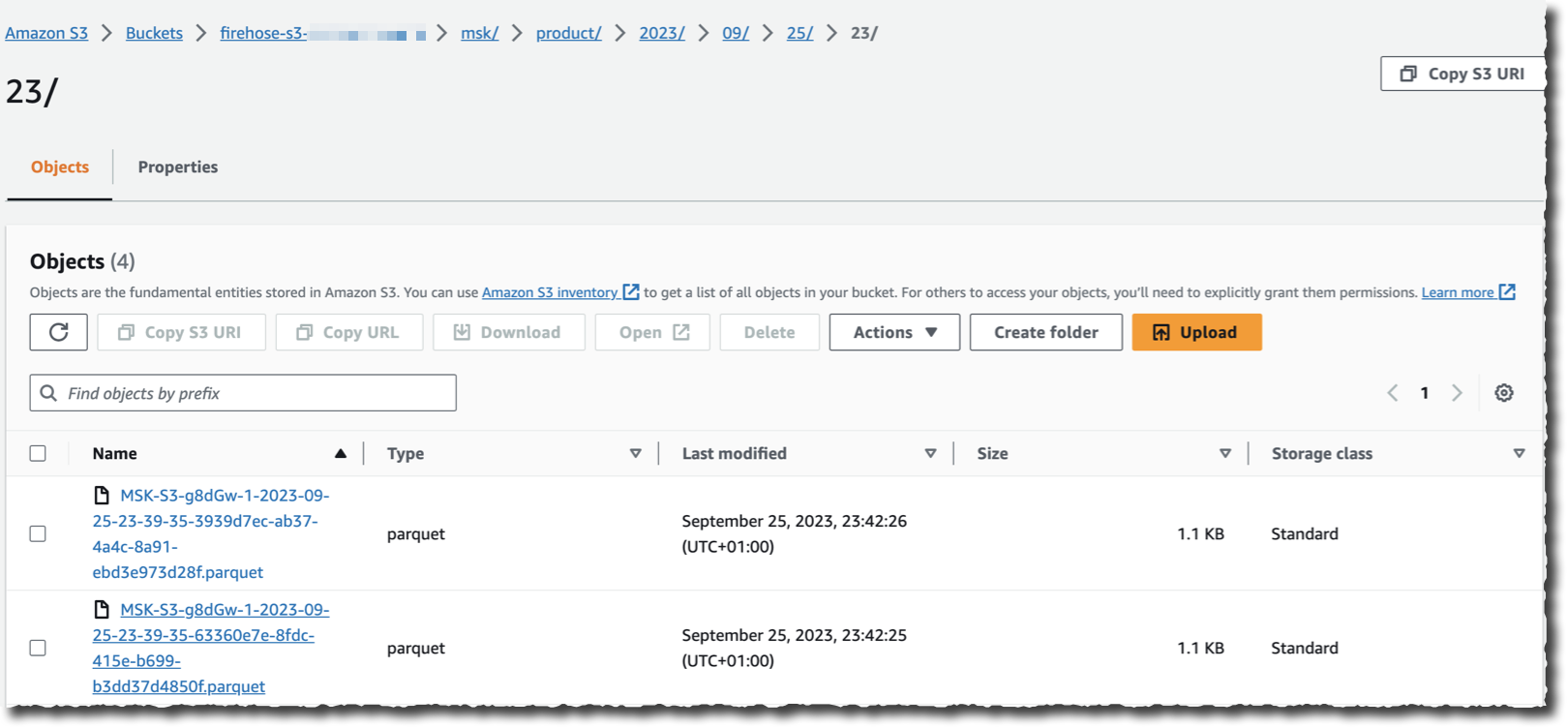
Finally, I enter the name of the destination Amazon S3 bucket. Again, when I cannot remember it, I use the Browse button to let the console guide me through my list of buckets. Optionally, I enter an S3 bucket prefix for the file names. For this demo, I enter aws-news-blog. When I don’t enter a prefix name, Kinesis Data Firehose uses the date and time (in UTC) as the default value.
Under the Buffer hints, compression and encryption section, I can modify the default values for buffering, enable data compression, or select the KMS key to encrypt the data at rest on Amazon S3.
When ready, I choose Create delivery stream. After a few moments, the stream status changes to  available.

Assuming there’s an application streaming data to the cluster I chose as a source, I can now navigate to my S3 bucket and see data appearing in the chosen destination format as Kinesis Data Firehose streams it.
As you see, no code is required to read, transform, and write the records from my Kafka cluster. I also don’t have to manage the underlying infrastructure to run the streaming and transformation logic.
Pricing and Availability.
This new capability is available today in all AWS Regions where Amazon MSK and Kinesis Data Firehose are available.
You pay for the volume of data going out of Amazon MSK, measured in GB per month. The billing system takes into account the exact record size; there is no rounding. As usual, the pricing page has all the details.
I can’t wait to hear about the amount of infrastructure and code you’re going to retire after adopting this new capability. Now go and configure your first data stream between Amazon MSK and Amazon S3 today.
[$] Moving the kernel to large block sizes
Post Syndicated from jake original https://lwn.net/Articles/945646/
Using larger block sizes in the kernel for I/O is a recurring topic in
storage and
block-layer circles. The topic came up in discussions
at the Linux Storage, Filesystem, Memory-Management and BPF Summit (LSFMM)
back in
May. One of the participants in those discussions, Hannes Reinecke, gave
a talk at Open Source Summit Europe 2023 with an overview of the reasons
behind using larger blocks for I/O, the current status of that work, and
where it all might lead from here.
AWS achieves QI2/QC2 qualification to host critical data and workloads from the Italian Public Administration
Post Syndicated from Giuseppe Russo original https://aws.amazon.com/blogs/security/aws-achieves-qi2-qc2-qualification-to-host-critical-data-and-workloads-from-the-italian-public-administration/
Amazon Web Service (AWS) is pleased to announce that it has achieved the QI2/QC2 qualification level, set out by the Italian National Cybersecurity Agency (ACN) in Determination No. 307/2022, for AWS cloud infrastructure and 130 AWS cloud services. The scope of this qualification level includes the management of Critical data and workloads for Italian public administration customers. Customers and partners who manage workloads identified as Critical, according to the rules set out in ACN Determination No. 307/2022, can now benefit from the qualification achieved by AWS.
Obtaining the ACN QI2/QC2 qualification for managing critical data and workloads means that AWS meets the 366 requirements for security, processing capacity, infrastructure reliability, and scalability of cloud services, including being certified according to security and compliance standards such as ISO 9001, ISO/IEC 27001:2013, ISO/IEC 27017:2015, ISO/IEC 27018:2019, Cloud Security Alliance – Star Level 2, ISO 22301, and ISO 20000.
Qualification of cloud infrastructure and services is an integral part of the Italian Cloud Strategy, issued by the Department for Digital Transformation and ACN. The strategy contains guidelines for migrating data and digital services of the Italian Public Administration to the cloud.
The Italian Cloud Strategy starts from the principle that public administrations manage data and workloads that operate at different levels of criticality. When migrating from an on-premises solution to the cloud, public administrations must identify which risk class their workloads and data belong to.
ACN has identified the following three classes of data in relation to the damage that could be caused to the country in the event of a breach in terms of confidentiality, integrity, and availability.
- Ordinary: Data and services whose deterioration does not cause the interruption of the state service nor, in any case, harm the economic and social wellbeing of the country.
- Critical: Data and services whose compromise could compromise the maintenance of important functions for society, health, safety, and the economic and social wellbeing of the country.
- Strategic: Data and services that, if compromised, can have an impact on national security.
Different levels of criticality require different levels of qualification according to the following scheme.

Figure 1. Different levels of criticality require different levels of qualification
Thanks to the presence of the AWS Europe (Milan) Region since April 2020, and the new QI2/QC2 qualification obtained by AWS, our customers and partners can now feel confident to develop innovative cloud services that manage the critical workloads of the Italian Public Administration that run on AWS cloud infrastructure. The qualification obtained by AWS will be available on the ACN Cloud Market Place in the next weeks.
Our customers can refer to the AWS QI2/QC2 qualification to confirm that the AWS control environment is designed and implemented appropriately. By receiving the qualification to manage Critical workloads, AWS demonstrates our commitment to meet the highest security expectations for cloud service providers set out by ACN.
As always, we value your feedback and questions. Reach out to the AWS Compliance team through the Contact Us page. To learn more about our other compliance and security programs, see AWS Compliance Programs.
If you have feedback about this post, submit comments in the Comments section below. If you have questions about this post, contact AWS Support.
Want more AWS Security news? Follow us on Twitter.
Network connectivity patterns for Amazon OpenSearch Serverless
Post Syndicated from Salman Ahmed original https://aws.amazon.com/blogs/big-data/network-connectivity-patterns-for-amazon-opensearch-serverless/
Amazon OpenSearch Serverless is an on-demand, auto-scaling configuration for Amazon OpenSearch Service. OpenSearch Serverless enables a broad set of use cases, such as real-time application monitoring, log analytics, and website search. OpenSearch Serverless lets you use OpenSearch without having to worry about scaling and managing an OpenSearch cluster. A collection can be accessed over the public internet or from your VPC. As you start accessing OpenSearch Serverless from different VPCs and accounts or from on premises, your connectivity patterns may change. In this post, we cover connectivity patterns and Domain Name System (DNS) resolution for your OpenSearch Serverless collection—whether accessed over the internet, within the VPC, within AWS, or from your on-premises location.
Foundational concepts
The following foundational concepts will help you better understand OpenSearch Serverless and DNS resolution.
Network access policy
The network access policy for OpenSearch Serverless determines whether the collection can be accessed over the internet or only through OpenSearch Serverless managed VPC endpoints. A single policy can be attached to multiple collections.
OpenSearch Serverless VPC endpoint
To access OpenSearch Serverless collections and dashboards privately from a VPC without using an internet gateway, you can create a VPC interface endpoint. When you create a VPC endpoint, it creates an elastic network interface (ENI) in each subnet that you enable for the VPC endpoint. These are requester-managed ENIs that serve as the entry point for traffic destined for the OpenSearch Serverless collection. When you create an OpenSearch Serverless VPC endpoint, the private DNS name option is enabled by default. This means that OpenSearch Serverless also creates an Amazon Route 53 private hosted zone and associates that with the VPC where the endpoint is created. This private hosted zone has a wildcard DNS record *.<region>.aoss.amazonaws.com pointing to the private DNS of the endpoint.
You create an OpenSearch Serverless VPC endpoint via the OpenSearch Serverless console or the OpenSearch Serverless API. You can’t create an OpenSearch Serverless VPC endpoint from the Amazon Virtual Private Cloud (Amazon VPC) console, although once created, you can see them on the VPC console as well.
Amazon Route 53 Resolver
Let’s understand what Amazon Route 53 Resolver does when an Amazon Elastic Compute Cloud (Amazon EC2) instance queries a DNS name. DNS queries originating from the VPC go to the Route 53 Resolver at the VPC+2 IP address. When a DNS query reaches the resolver, it checks if there are any Route 53 forward rules. If it matches, then it forwards the query to the DNS server provided by that rule. If the query remains unresolved, Route 53 Resolver proceeds to check the private hosted zones associated with the originating VPC. If it still remains unresolved, then it checks for VPC DNS, which helps to resolve EC2 DNS names. Lastly, if the query still isn’t resolved, Route 53 Resolver checks the public DNS. The following diagram illustrates this order or operations.

Route 53 Resolver inbound endpoints
Workloads utilizing resources both in a VPC and on premises need to resolve DNS records hosted on-premises and resources hosted in the VPC. With Route 53 Resolver inbound endpoints, you can resolve DNS queries to your VPC from your on-premises network or another VPC.
In the following sections, we provide an overview of connectivity patterns and DNS resolution.
Access an OpenSearch Serverless collection from Amazon EC2 (via internet gateway)
The following figure demonstrates the connectivity pattern to access an OpenSearch Serverless collection over the internet. The collection has an access type set to public, which allows authorized users to connect to the collection over the internet. An EC2 instance within the VPC can establish a connection to the collection via the internet gateway, and users outside the VPC can also access this collection over the internet.

The workflow has the following steps, as indicated in the preceding diagram:
A. The EC2 instance performs a DNS lookup to Route 53 Resolver at a VPC+2 IP address. Route 53 Resolver returns the public IP addresses of the OpenSearch Serverless collection.
B. The EC2 instance sends a data request via an internet gateway to the OpenSearch Serverless collection using this public IP address.
C. An external client resolves to the public IP addresses of the OpenSearch Serverless collection and reaches it via the internet.
Now let’s perform a dig command for the collection or dashboard URL from the EC2 instance, and we observe that it’s resolving to a public IP address.
The following command uses an OpenSearch Serverless collection:
The following command uses an OpenSearch dashboard:
Now that you have implemented an OpenSearch Serverless collection with a network access policy as public, you can make the same collection accessible privately within the VPC. To achieve this, complete the following steps:
- Modify the network access policy of the collection and change the access type to VPC.
- Select the option Create VPC endpoints.

- Choose the VPC and at least two subnets where you would like to have a VPC endpoint ENI for high availability.
- Choose Confirm to create the VPC endpoint.

- Lastly, select the VPC endpoint and update the policy.

With the creation of the VPC endpoint, a Route 53 private hosted zone is also created within your account and associated with your VPC. In this setup, a CNAME record *.us-east-1.aoss.amazonaws.com is created to direct to the Regional AWS PrivateLink endpoint, as depicted in the following screenshot.

Due to the private hosted zone associated with the VPC, Route 53 Resolver gives preference to the private hosted zone to resolve any DNS query originating from the VPC. DNS requests for the OpenSearch Serverless collection originating from the EC2 instance get resolved using this associated private hosted zone and resolve to the private IP addresses of the VPC endpoint, which allows Amazon EC2 to connect to the serverless collection via VPC endpoints vs. the internet gateway. We expand on this in the following section.
Access an OpenSearch Serverless collection from Amazon EC2 (via interface VPC endpoints)
The following figure demonstrates the connectivity pattern to access an OpenSearch Serverless collection privately from the VPC. The collection has an access type set to VPC endpoint, restricting access solely from the resources within the VPC via the VPC endpoint and preventing external users from connecting. With the creation of the VPC endpoint, a private hosted zone is also associated with this VPC. An EC2 instance within the VPC can establish a connection with the collection using the VPC endpoint, but resources outside of the VPC don’t have access to this collection because of the network access policy.

The workflow consists of the following steps:
A. The EC2 instance performs a DNS lookup to Route 53 Resolver at a VPC+2 IP address. Route 53 Resolver returns the private IP addresses of the VPC endpoint because there is a private hosted zone associated with the VPC containing a CNAME record.
B. The EC2 instance sends a data request via the VPC interface endpoint to the OpenSearch Serverless collection.
C. An external client resolves to the public IP addresses of the OpenSearch Serverless collection but is unable to reach it because the network policy restricts to the VPC.
Now let’s perform a dig command for the collection or dashboard URL from the EC2 instance, and we observe that it’s resolving to the private IP addresses belonging to the VPC endpoints.
Use the following code for an OpenSearch Serverless collection:
Use the following code for an OpenSearch dashboard:
Access an OpenSearch Serverless collection from many VPCs (via interface VPC endpoints) with a VPC endpoint in each VPC
The following figure demonstrates the connectivity pattern to use the same VPC endpoint to connect to multiple OpenSearch Serverless collections. In this scenario, a VPC endpoint is created in each VPC to enable EC2 instances within the VPCs to utilize the VPC endpoint as the connectivity path to OpenSearch Serverless. A private hosted zone is auto generated for each endpoint and associated with the corresponding VPC. Network policies of OpenSearch Serverless collections are updated to allow both VPC Endpoint-1 and VPC Endpoint-2, which allows the EC2 instance in VPC-1 to access both collections via VPC Endpoint-1 and EC2 instances in VPC-2 to access both collections via VPC Endpoint-2.

The workflow consists of the following steps:
A. The EC2 instance performs a DNS lookup to Route 53 Resolver at a VPC+2 IP address. Route 53 Resolver returns the private IP addresses of the VPC endpoint (the EC2 instance in VPC-1 gets the IP address of VPC Endpoint-1 and the EC2 instance in VPC-2 gets the IP address of VPC Endpoint-2), because there is a private hosted zone associated with each of the VPCs containing a CNAME record.
B. The EC2 instance sends a data request via the VPC interface endpoint to the OpenSearch Serverless collection.
Access an OpenSearch Serverless collection from many VPCs (via interface VPC endpoints) with a VPC endpoint in a centralized VPC
In the previous connectivity pattern, we had one endpoint in each VPC through which VPC resources accessed OpenSearch Serverless collections. Many organizations would like to maintain control of these endpoints and keep these in a centralized VPC.
The following figure demonstrates the connectivity pattern to use a centralized VPC endpoint to connect to multiple OpenSearch Serverless collections from multiple VPCs. In this scenario, a VPC interface endpoint is created in a centralized VPC. A private hosted zone is auto generated for this VPC endpoint and associated with the centralized VPC, and then manually associated with VPC-1 and VPC-2. The DNS query for OpenSearch Serverless collections from VPC-1 and VPC-2 gets resolved to the centralized VPC endpoint due to the private hosted zone association. Network policies for both collections allow access from the centralized VPC endpoint only. All three VPCs (centralized, VPC-1, and VPC-2) are connected via AWS Transit Gateway and route tables have routes to direct traffic between VPC-1 and VPC-2 to the centralized VPC and vice versa.

The workflow consists of the following steps:
A. The EC2 instance performs a DNS lookup to Route 53 Resolver at a VPC+2 IP address. Route 53 Resolver returns the private IP addresses of the centralized VPC endpoint, because there is a private hosted zone associated with each VPC containing a CNAME record.
B. The EC2 instance sends a data request to the Transit Gateway ENI in its own VPC. The Transit Gateway route table is checked and the data request is forwarded to the Transit Gateway ENI in the centralized VPC. The Transit Gateway ENI in the centralized VPC sends it to the OpenSearch Serverless collection via the VPC interface endpoint.
Access an OpenSearch Serverless collection from on premises (via AWS Site-to-Site VPN or AWS Direct Connect)
The following figure demonstrates the connectivity pattern for accessing OpenSearch Serverless collections from on premises. You can use either AWS Direct Connect or AWS Site-to-Site VPN to establish connectivity between on-premises and AWS resources. In the following example, Direct Connect is used for the connectivity between AWS and on premises. An OpenSearch Serverless VPC endpoint is created in the VPC, and a private hosted zone is automatically generated and associated with this VPC. The network policy of the OpenSearch Serverless collection is updated to allow connectivity only from the VPC endpoint.
To access these OpenSearch Serverless collections privately from the on-premises environment, resources need to resolve the OpenSearch Serverless collection DNS to the OpenSearch Serverless VPC endpoint IP address. By default, OpenSearch Serverless DNS resolves to the public IP addresses and attempts to access OpenSearch Serverless via the internet. To ensure that OpenSearch Serverless is accessed via the VPC endpoint from on premises, you need to ensure that DNS queries are resolved to a VPC endpoint’s private IP address. Resources inside the VPC use Route 53 Resolver, available at a VPC+2 IP address, to resolve these queries to the VPC endpoint. Route 53 Resolver checks the associated private hosted zone to resolve the query to the VPC endpoint. However, the VPC+2 IP address is not accessible from on premises. To address this, you can utilize the Route 53 Resolver inbound endpoint.
To achieve this, you can create an inbound endpoint in your VPC by following the steps outlined in Configuring inbound forwarding, and then update the on-premises DNS server to forward all the DNS requests for *.<region>.aoss.amazonaws.com to the IP address of the Route 53 Resolver inbound endpoint. When the on-premises client obtains the IP address of the VPC endpoint, it can use Direct Connect or Site-to-Site VPN to establish a private connection to the OpenSearch Serverless collection.

The workflow contains the following steps:
A. The on-premises client sends a DNS lookup to the on-premises DNS resolver. The on-premises DNS resolver forwards this request to the Route 53 Resolver inbound endpoint. The Route 53 Resolver inbound endpoint sends a DNS lookup to Route 53 Resolver at a VPC+2 IP address. Route 53 Resolver returns the private IP addresses of the VPC endpoint, because there is a private hosted zone associated with this VPC containing a CNAME record.
B. The on-premises client sends a data request to the OpenSearch Serverless collection, which routes via Direct Connect or Site-to-site VPN to the VPC interface endpoint and finally to the OpenSearch Serverless collection.
Conclusion
In this post, we showed you various connectivity patterns for OpenSearch Serverless. We covered the use of hybrid DNS and using a Route 53 Resolver inbound endpoint to allow connectivity from on premises for OpenSearch Serverless. You can choose from various centralization models for reaching multiple OpenSearch Serverless collections within the AWS Cloud or from on-premises locations. Get started today by connecting to OpenSearch Serverless from the various network patterns we discussed.
About the authors
 Salman Ahmed is a Sr. Technical Account Manager in AWS Enterprise Support. He enjoys working with Enterprise Support customers to help them with design, implementation and supporting cloud infrastructure. He also has a passion for networking services and with 12+ years of experience, he leverages that to help customers with adoption of AWS Transit Gateway, AWS Direct Connect and various other AWS networking services.
 Ankush Goyal is Enterprise Support Lead in AWS Enterprise Support who helps enterprise support customers streamline their cloud operations on AWS. He is a results-driven IT professional with over 18 years of experience.
 Rohit Aswani is a Senior Specialist Solutions Architect focussed on Networking at AWS, where he helps customers build and design scalable, highly-available, secure, resilient and cost effective networks. He holds a MS in Telecommunication Systems Management from Northeastern University, specializing in Computer Networking. In his spare time, Rohit enjoys hiking, traveling and exploring new coffee places.
Improved resiliency with cluster manager task throttling for Amazon OpenSearch Service
Post Syndicated from Dhwanil Patel original https://aws.amazon.com/blogs/big-data/improved-resiliency-with-cluster-manager-task-throttling-for-amazon-opensearch-service/
Amazon OpenSearch Service is a managed service that makes it simple to secure, deploy, and operate OpenSearch clusters at scale in the AWS Cloud. Amazon OpenSearch clusters are comprised of data nodes and cluster manager nodes. The cluster manager nodes elect a leader among themselves. The leader node is the authority on the metadata in the cluster, which is called cluster state. Any changes to the cluster state are processed by the leader node and broadcasted to all of the nodes in the cluster. The data nodes enqueue a new cluster-level task for any cluster state change like creation of an index, dynamic put-mappings, shard started, etc. in the cluster manager’s unbounded queue. The tasks waiting in this queue are called pending tasks. Because it’s unbounded, a large number of pending tasks can be queued, which overloads the leader node. This can affect the leader’s performance and may also in turn affect the stability and availability of the whole cluster.
We have introduced a throttling mechanism for cluster manager nodes to provide protection against a large number of pending tasks. It acts during task submission to the leader node. This feature is available for Amazon OpenSearch engine version 1.3 and above in Amazon OpenSearch Service.
Cluster manager task throttling
Cluster manager task throttling is a mechanism to protect the cluster manager against submission of too many resource-intensive cluster state update tasks from other nodes. For tasks like put-mapping, data nodes have an existing throttling mechanism for cluster-state tasks that helps avoid overload of the cluster manager. For example, if the cluster manager can handle 10 K requests and the domain has 10 data nodes, then each data node gets a throttle at 1,000 put-mapping requests. If the domain grows to 100 data nodes, then each data node must throttle at 100 requests. To avoid having to modify these throttle limit whenever the cluster changes the number of data nodes and to support more task types, we ‘ve introduced throttling at cluster manager node for self-protection.
The cluster state update tasks are of different types ( create-index, put-mapping, and more) and this throttling mechanism rejects a task based on its type. For any incoming task, the cluster manager evaluates the total number of tasks of the same type in the pending task queue. If this number exceeds the threshold for a task type, then the cluster manager rejects the incoming task.
Amazon OpenSearch Service configures different throttling thresholds for different task types and throttling acts independently on each task type. Rejecting a particular task doesn’t affect other tasks of a different type. For example, if the cluster manager rejects a put-mapping task, it can still accept a concurrent create-index task.
All of the tasks generated by data plane APIs( _mapping/, _setting/ and more) have been onboarded for throttling and are listed here.
When the cluster manager rejects a task, the data node performs retries with exponential back off to resubmit the task to the cluster manager until it is successfully submitted. If retries are unsuccessful within the timeout period, then Amazon OpenSearch returns a cluster timeout error.
Sample of error
Handling time out errors
The throttling exception is acted upon by data nodes; they perform the retries on throttled task. If API times out during throttling period, you’ll get process_cluster_event_timeout_exception , which is a 503 error. This is the same error that was thrown earlier as well when tasks are timing out in the cluster manager node’s queue. You can retry the API calls with timeout errors.
This solution will improve this feature by exposing the throttling exception directly as an API error.
Monitoring throttling
You can monitor the detailed throttling stats using the _nodes/stats API.
You can use the cluster_manager_throttling section in the _nodes/stats response to track, which tasks are getting throttled and how many tasks has been throttled.
Sample response
Conclusion
In this post, we showed you how a throttling mechanism for task submission to the cluster manager node makes it more resilient to a high number of pending tasks in Amazon OpenSearch Service, where we have fine-tuned the thresholds per cluster.
Cluster manager throttling is available in Amazon OpenSearch, and we are always looking for external contributions. You can refer to the RFC (Request For Comment) to get started.
About the Authors
![]() Dhwanil Patel is a Software Developer Engineer working on Amazon OpenSearch Service. He likes to contribute to open-source software development, and is passionate about distributed systems.
Dhwanil Patel is a Software Developer Engineer working on Amazon OpenSearch Service. He likes to contribute to open-source software development, and is passionate about distributed systems.
![]() Shweta Thareja is a Principal Engineer working on Amazon OpenSearch Service. She is interested in building distributed and autonomous systems. She is a maintainer and an active contributor to OpenSearch.
Shweta Thareja is a Principal Engineer working on Amazon OpenSearch Service. She is interested in building distributed and autonomous systems. She is a maintainer and an active contributor to OpenSearch.
![]() Jon Handler is a Senior Principal Solutions Architect at Amazon Web Services based in Palo Alto, CA. Jon works closely with OpenSearch and Amazon OpenSearch Service, providing help and guidance to a broad range of customers who have search and log analytics workloads that they want to move to the AWS Cloud. Prior to joining AWS, Jon’s career as a software developer included 4 years of coding a large-scale, ecommerce search engine. Jon holds a Bachelor of the Arts from the University of Pennsylvania, and a Master of Science and a PhD in Computer Science and Artificial Intelligence from Northwestern University.
Jon Handler is a Senior Principal Solutions Architect at Amazon Web Services based in Palo Alto, CA. Jon works closely with OpenSearch and Amazon OpenSearch Service, providing help and guidance to a broad range of customers who have search and log analytics workloads that they want to move to the AWS Cloud. Prior to joining AWS, Jon’s career as a software developer included 4 years of coding a large-scale, ecommerce search engine. Jon holds a Bachelor of the Arts from the University of Pennsylvania, and a Master of Science and a PhD in Computer Science and Artificial Intelligence from Northwestern University.
How Bad Could BA.2.86 Get?
Post Syndicated from The Atlantic original https://www.youtube.com/watch?v=dGkC65kmdxA
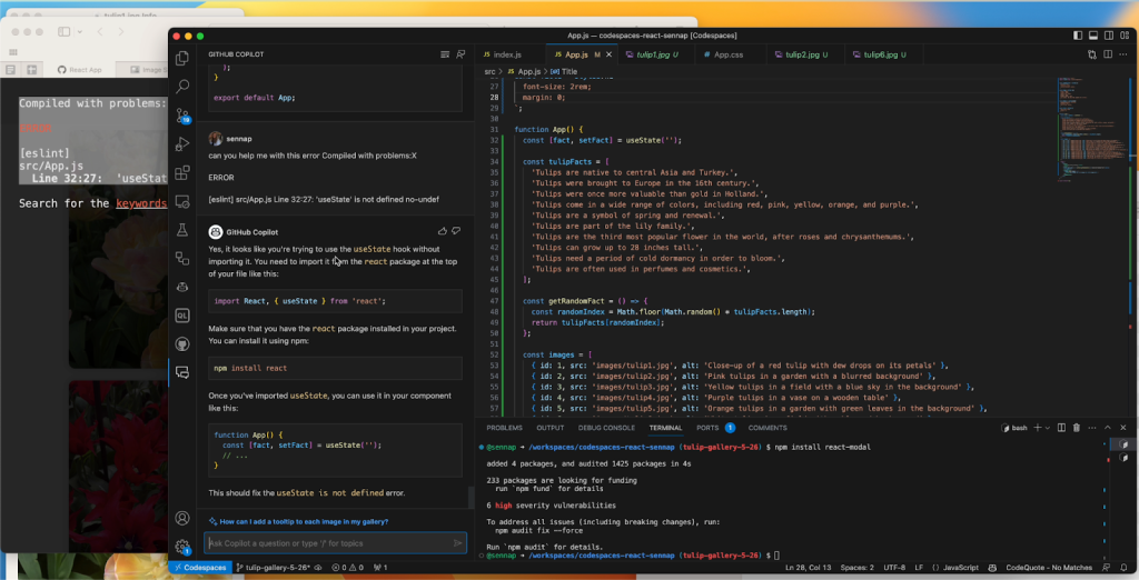
How I used GitHub Copilot Chat to build a ReactJS gallery prototype
Post Syndicated from Senna Parsa original https://github.blog/2023-09-27-how-i-used-github-copilot-chat-to-build-a-reactjs-gallery-prototype/
Ever since we announced GitHub Copilot Chat in March this year, I’ve been thinking a lot about how it’s improving developer happiness and overall satisfaction while coding. Especially for junior developers looking to upskill, or those in the learning phase of diving into a new framework, GitHub Copilot Chat can be such a valuable tool to have in your back pocket.
ICYMI, all GitHub Copilot for Individuals users now have access to GitHub Copilot Chat beta!
The capabilities of GitHub Copilot Chat
With GitHub Copilot Chat, you can now interface with Copilot as a context-aware conversational assistant right in the IDE, allowing you to execute some of the most complex tasks with simple prompts. This goes beyond GitHub Copilot’s original capabilities, which focused on autocompletion and translating natural language comments into code. Now, developers can not only get code suggestions in-line, but they can ask Copilot questions directly, get explanations, offer prompts for code, and more, all while staying in the IDE—and in the flow.
Navigating a new framework (and saving time)
Recently, I was preparing a conference talk and demo about ReactJS, and I had to think a bit about what kind of app I wanted to make with the help of Copilot Chat. Since photography is a hobby of mine, I decided to make a photo gallery of the tulip fields and flower shows around Amsterdam. In the end, I went through a couple different versions of this photo gallery with Copilot Chat. Using a probabilistic model, which is currently based on OpenAI’s GPT-3.5-turbo, it found the best suggestion for me based on how I prompted it, including the question I asked, the code I’d started writing, and other open tabs in my IDE.
It had been a long time since I had used React, so it probably would’ve taken me a few days of searching and trial and error before coming up with something decent. But with Copilot Chat, each iteration of my photo gallery only took me about 20-30 minutes to go through.
Making prototypes and generating new code
What I most enjoyed about using Copilot Chat to create something new was discovering multiple ways I could implement my component. I didn’t have to leave my IDE and search for advice or a component to use because Copilot would suggest something in real time. If it offered me a suggestion that didn’t work out well, I could give it feedback on why that suggestion didn’t work, which enabled it to offer suggestions that better suited my needs.
Despite working in an unfamiliar framework, Copilot Chat enabled me to immediately start churning out my ideas, which was incredibly satisfying. It was empowering to discover that I can get something done so much faster than what I would have anticipated without any help.
This idea of looking for external help and examples to understand code has been part of the learning process since well before we had AI pair programming tools. I remember when I was first starting in my career and discovering all these new frameworks. I would spend hours, days, weeks doing tutorials and learning about different ways of implementing things. I would learn by copying and pasting things I saw on StackOverflow and seeing how they fit in with the rest of my code (or by chatting with my buddy that I shared a cubicle with at the time).
A lot of the time, these code snippets didn’t even work, but having something to start with really helped with the learning process and that excitement propelled me forward to the next step. This is exactly the magic I felt when using Copilot Chat—while being able to get a contextual suggestion that actually worked and helped me quickly progress to the next thing. Not to mention the amount of time and energy I saved by staying within the context of VS Code instead of searching through websites and other comments online (and avoiding some stress caused by the sentiment of some Stack Overflow comments).
GitHub Copilot Chat in action
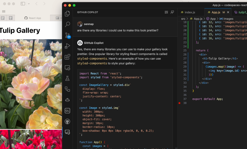
When it came time to build my photo gallery, I used Copilot Chat to get suggestions for popular React libraries I could use. There were a few of them that I checked out in separate iterations of the gallery but styled components seems to be the easiest one for me to configure.
I wanted to include a modal as well, so I asked Copilot if the styled components library supported modals. I was really surprised that it knew exactly how to utilize the modal component of the library and how to pass the props in and handle the onClick functionality from the get-go.
In the video, you may notice that it initially gives me a generic suggestion with some boilerplate examples of how to define a modal component and how to reference it from another file. I then asked it to iterate on that suggestion and give me something more specific to how I defined my gallery. This is important because the power of GitHub Copilot is really in the prompt that you provide it: the more fine-tuned the information, the more powerful its suggestions will be. For further reading, check out these prompt tips and tricks for leveraging GitHub Copilot effectively as well as this post on how we compose prompts at GitHub.
Testing out a UI change based on a natural language prompt
When I first tried rendering a modal, that close button was out of view on the top right corner of the screen. This isn’t too difficult to do if you’re regularly developing front-end. Full transparency: I would have needed to Google how to fix this since I just don’t remember how to and CSS is hard! I was shocked that just by asking Copilot Chat to center the “X” button in the modal, it gave me a better suggestion with some new CSS to add display properties to the button that adjust it to my intention. With Copilot Chat, I got the fix I needed without having to leave the IDE or break my flow.
Making accessibility improvements
I have a background in web accessibility and I knew there would be some improvements needed to make the modals interactive with proper focus handling. There are many facets to making a component accessible and it’s important to strategize early on. Best practices include working with accessibility linting tools, and also specialists that can help you balance constraints at the start of the design and development process.
Copilot Chat can be a great addition to those tools by pointing you in the right direction to fixing accessibility issues. In the case of my gallery, the images were not presenting themselves as interactive to keyboard or screen reader users (or, even visually, which goes to show that accessibility makes products better for everyone!). I asked Copilot Chat what it recommended for me to improve the interactivity of the images. The video below illustrates the suggestions it provided around using tabindex, aria attributes, and handling keydown events.
There are, of course, other accessibility considerations to be made here. At some point I decided to make each of the images button elements with a background image, since generally it’s better to use semantic HTML. I then carried on with the rest of my work to manage the focus correctly when opening and closing the modal, as well as making sure only the visible or focused content is presented to a screen reader.
Troubleshooting errors
I was also surprised by Copilot Chat’s ability to help me debug my project whenever I came across an error message. I’d just paste the error into the chat window and GitHub Copilot would offer an explanation for what went wrong and an alternative approach so I could fix the bug quickly and move on.
Writing tests
Knowing that GitHub Copilot can suggest bug fixes, I also wanted to see how it would suggest I write tests for my code. You can ask Copilot Chat for all sorts of test cases, as well as just what kind of testing framework would make the most sense for your application.
In another iteration of my gallery, I used GitHub Copilot to help me render a countdown to the next opening of Tulip season (I went with March 21, 2024, when the tulip festival starts). I decided to make use of the new Copilot Chat slash commands that make it simple to highlight a function and prompt it to help me create some test cases. It suggested using the React testing library for rendering, as well as some methods from Jest to simulate the passage of time and make sure the passing days are represented correctly. From there, I learned about the Jest framework’s Timer Mocks and best practices for testing for fake timers.
Without GitHub Copilot and this new chat feature, navigating a test framework and relying solely on their documentation would have taken even more time.
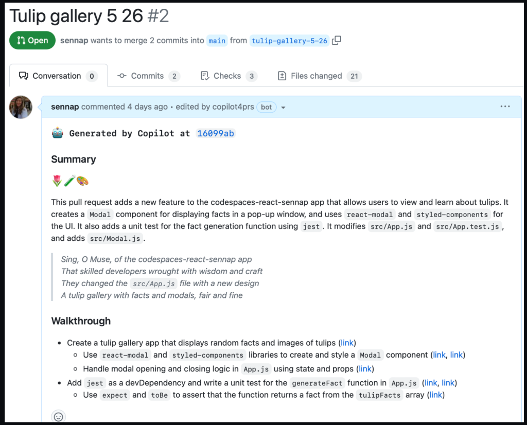
Summarizing my changes with GitHub Copilot for pull requests
Lastly, I used GitHub Copilot for pull requests to help summarize all the changes I made in a pull request. It gave me a summary of my changes, a walk through of each of the diffs relating to those changes, and even a poem about my application.
All of this is to show how Copilot Chat and GitHub Copilot for pull requests made the entire coding process much more enjoyable for me while working in an unfamiliar framework—from the initial idea phase to submitting a pull request.

Potential limitations and considerations
While the productivity increases for GitHub Copilot are amazing, there are valid concerns around the quality of code AI paired programming tools suggest and the danger of blindly trusting them. That’s why it’s important to remember that you, the developer, is ultimately the pilot. I think of using GitHub Copilot to be similar to pair programming with another developer: it helps me work faster, but I still need to verify the suggestions it’s giving me to ensure they meet my requirements.
While GitHub Copilot has numerous filters in place to avoid suggestions with vulnerabilities, it’s still important to review and test before deploying. As with any code you did not independently originate, you should ensure code suggestions go through proper code review, code security, and code quality channels to maintain the standards of your team.
The post How I used GitHub Copilot Chat to build a ReactJS gallery prototype appeared first on The GitHub Blog.
Best Zigbee IR blaster for Home Assistant, but…
Post Syndicated from BeardedTinker original https://www.youtube.com/watch?v=3Qy0jrL14vY
Inside the eye of a lobster with Kristy Hamilton #SHORTS
Post Syndicated from Talks at Google original https://www.youtube.com/watch?v=oajo-hAKGuM
Minisforum NPB7 Intel Core i7 Mini PC with Dual 2.5GbE LAN
Post Syndicated from Patrick Kennedy original https://www.servethehome.com/minisforum-npb7-intel-core-i7-mini-pc-with-dual-2-5gbe-lan/
In our Minisforum NPB7 review, we found a surprisingly good Intel mini PC with some design choices that we were not expecting
The post Minisforum NPB7 Intel Core i7 Mini PC with Dual 2.5GbE LAN appeared first on ServeTheHome.
Let’s Architect! Leveraging SQL databases on AWS
Post Syndicated from Luca Mezzalira original https://aws.amazon.com/blogs/architecture/lets-architect-leveraging-sql-databases-on-aws/
SQL databases in Amazon Web Services (AWS), using services like Amazon Relational Database Service (Amazon RDS) and Amazon Aurora, offer software architects scalability, automated management, robust security, and cost-efficiency. This combination simplifies database management, improves performance, enhances security, and allows architects to create efficient and scalable software systems.
In this post, we introduce caching strategies and continue with real case studies that use services like Amazon ElastiCache or Amazon MemoryDB in real workloads where customers share the reasoning behind their approaches. It’s very important to understand the context for leveraging a specific solution or pattern, and these resources answer many commonly asked questions.
Build scalable multi-tenant databases with Amazon Aurora
For software architects and developers, striking the right balance between operational complexity and cost efficiency is a perpetual challenge. Often, provisioning a separate database for each workload is the gold standard, offering unmatched isolation and granular operational controls. However, it’s not always the most cost-effective or operationally manageable approach. Through a real-world success story, we explore how Aurora played a pivotal role in helping VMware Aria Cost, powered by CloudHealth, consolidate a staggering 166 self-managed MySQL databases onto 62 Aurora clusters.
Take me to this re:Invent 2022 video!

A migration process to move a MySQL database from self-managed to fully managed with Amazon Aurora
Amazon RDS Blue/Green Deployments, Optimized Writes & Optimized Reads
Amazon RDS Blue/Green Deployments revolutionizes the way you handle database updates, ensuring safety and simplicity, often achieving rapid updates in just a minute, with zero data loss. Meanwhile, Amazon RDS Optimized Writes turbocharges write transaction throughput by as much as double, without any additional extra cost. Amazon RDS Optimized Reads steps in to deliver a significant boost to database performance, processing queries up to 50% faster.
Discover how to leverage these capabilities of Amazon RDS in this one-hour video from re:Invent 2022.
Take me to this re:Invent 2022 video!

Amazon RDS Blue/Green Deployments in action
Designing a DR strategy on Amazon RDS for SQL Server
In the world of mission-critical workloads, the importance of a robust disaster recovery (DR) strategy cannot be overstated. It’s the lifeline that ensures databases stay operational, even in the face of unexpected events. Discover the intricacies of crafting a dependable, cross-Region DR strategy tailored to Amazon RDS for SQL Server.
In this AWS Developers session, we uncover the best practices for efficiently managing and monitoring these cross-Region read replicas. From proactive monitoring to fine-tuning, you’ll gain the insights needed to keep your DR strategy finely tuned.
Take me to this AWS Developers video!

How to design a DR strategy using Amazon RDS
Deep dive into Amazon Aurora and its innovations
Aurora represents a paradigm shift in relational databases, boasting an architecture that decouples computational processes from data storage. It introduces advanced features, such as Global Database and low-latency read replicas, redefining the landscape of database management.
This modern database service excels in performance, scalability, and high availability on a large scale, offering compatibility with both MySQL and PostgreSQL open-source editions. Additionally, it provides an array of developer tools tailored for serverless and machine learning-driven applications.
This re:Invent 2022 session is an in-depth exploration of some of Aurora’s most compelling features, including Aurora Serverless v2 and Global Database. We also share the most recent innovations aimed at enhancing performance, scalability, and security while streamlining operational processes.
Take me to this re:Invent 2022 video!

A glance of one of the features of Amazon Aurora Global Database
See you next time!
Thanks for joining us today to explore leveraging SQL databases! We’ll see you in two weeks when we talk about batch processing workloads.
To find all the blogs from this series, check out the Let’s Architect! list of content on the AWS Architecture Blog.
Home Assistant 2023.10 Release Party
Post Syndicated from Home Assistant original https://www.youtube.com/watch?v=-GDonruFfKc
You can now use WebGPU in Cloudflare Workers
Post Syndicated from André Cruz original http://blog.cloudflare.com/webgpu-in-workers/

The browser as an app platform is real and stronger every day; long gone are the Browser Wars. Vendors and standard bodies have done amazingly well over the last years, working together and advancing web standards with new APIs that allow developers to build fast and powerful applications, finally comparable to those we got used to seeing in the native OS' environment.
Today, browsers can render web pages and run code that interfaces with an extensive catalog of modern Web APIs. Things like networking, rendering accelerated graphics, or even accessing low-level hardware features like USB devices are all now possible within the browser sandbox.
One of the most exciting new browser APIs that browser vendors have been rolling out over the last months is WebGPU, a modern, low-level GPU programming interface designed for high-performance 2D and 3D graphics and general purpose GPU compute.
Today, we are introducing WebGPU support to Cloudflare Workers. This blog will explain why it's important, why we did it, how you can use it, and what comes next.
The history of the GPU in the browser
To understand why WebGPU is a big deal, we must revisit history and see how browsers went from relying only on the CPU for everything in the early days to taking advantage of GPUs over the years.
In 2011, WebGL 1, a limited port of OpenGL ES 2.0, was introduced, providing an API for fast, accelerated 3D graphics in the browser for the first time. By then, this was somewhat of a revolution in enabling gaming and 3D visualizations in the browser. Some of the most popular 3D animation frameworks, like Three.js, launched in the same period. Who doesn't remember going to the (now defunct) Google Chrome Experiments page and spending hours in awe exploring the demos? Another option then was using the Flash Player, which was still dominant in the desktop environment, and their Stage 3D API.
Later, in 2017, based on the learnings and shortcomings of its predecessor, WebGL 2 was a significant upgrade and brought more advanced GPU capabilities like compute shaders and more flexible textures and rendering.
WebGL, however, has proved to be a steep and complex learning curve for developers who want to take control of things, do low-level 3D graphics using the GPU, and not use 3rd party abstraction libraries.
Furthermore and more importantly, with the advent of machine learning and cryptography, we discovered that GPUs are great not only at drawing graphics but can be used for other applications that can take advantage of things like high-speed data or blazing-fast matrix multiplications, and one can use them to perform general computation. This became known as GPGPU, short for general-purpose computing on graphics processing units.
With this in mind, in the native desktop and mobile operating system worlds, developers started using more advanced frameworks like CUDA, Metal, DirectX 12, or Vulkan. WegGL stayed behind. To fill this void and bring the browser up to date, in 2017, companies like Google, Apple, Intel, Microsoft, Kronos, and Mozilla created the GPU for Web Community Working Group to collaboratively design the successor of WebGL and create the next modern 3D graphics and computation capabilities APIs for the Web.
What is WebGPU
WebGPU was developed with the following advantages in mind:
- Lower Level Access – WebGPU provides lower-level, direct access to the GPU vs. the high-level abstractions in WebGL. This enables more control over GPU resources.
- Multi-Threading – WebGPU can leverage multi-threaded rendering and compute, allowing improved CPU/GPU parallelism compared to WebGL, which relies on a single thread.
- Compute Shaders – First-class support for general-purpose compute shaders for GPGPU tasks, not just graphics. WebGL compute is limited.
- Safety – WebGPU ensures memory and GPU access safety, avoiding common WebGL pitfalls.
- Portability – WGSL shader language targets cross-API portability across GPU vendors vs. GLSL in WebGL.
- Reduced Driver Overhead – The lower level Vulkan/Metal/D3D12 basis improves overhead vs. OpenGL drivers in WebGL.
- Pipeline State Objects – Predefined pipeline configs avoid per-draw driver overhead in WebGL.
- Memory Management – Finer-grained buffer and resource management vs. WebGL.
The “too long didn't read” version is that WebGPU provides lower-level control over the GPU hardware with reduced overhead. It's safer, has multi-threading, is focused on compute, not just graphics, and has portability advantages compared to WebGL.
If these aren't reasons enough to get excited, developers are also looking at WebGPU as an option for native platforms, not just the Web. For instance, you can use this C API that mimics the JavaScript specification. If you think about this and the power of WebAssembly, you can effectively have a truly platform-agnostic GPU hardware layer that you can use to develop platforms for any operating system or browser.
More than just graphics
As explained above, besides being a graphics API, WebGPU makes it possible to perform tasks such as:
- Machine Learning – Implement ML applications like neural networks and computer vision algorithms using WebGPU compute shaders and matrices.
- Scientific Computing – Perform complex scientific computation like physics simulations and mathematical modeling using the GPU.
- High Performance Computing – Unlock breakthrough performance for parallel workloads by connecting WebGPU to languages like Rust, C/C++ via WebAssembly.
WGSL, the shader language for WebGPU, is what enables the general-purpose compute feature. Shaders, or more precisely, compute shaders, have no user-defined inputs or outputs and are used for computing arbitrary information. Here are some examples of simple WebGPU compute shaders if you want to learn more.
WebGPU in Workers
We've been watching WebGPU since the API was published. Its general-purpose compute features perfectly fit our Workers' ecosystem and capabilities and align well with our vision of providing our customers multiple compute and hardware options and bringing GPU workloads to our global network, close to clients.
Cloudflare also has a track record of pioneering support for emerging web standards on our network and services, accelerating their adoption for our customers. Examples of these are Web Crypto API, HTTP/2, HTTP/3, TLS 1.3, or Early hints, but there are more.
Bringing WebGPU to Workers was both natural and timely. Today, we are announcing that we have released a version of workerd, the open-sourced JavaScript / Wasm runtime that powers Cloudflare Workers, with WebGPU support, that you can start playing and developing applications with, locally.
Starting today anyone can run this on their personal computer and experiment with WebGPU-enabled workers. Implementing local development first allows us to put this API in the hands of our customers and developers earlier and get feedback that will guide the development of this feature for production use.
But before we dig into code examples, let's explain how we built it.
How we built WebGPU on top of Workers
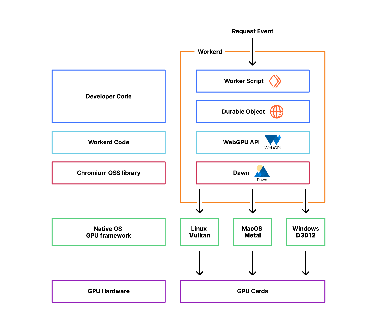
To implement the WebGPU API, we took advantage of Dawn, an open-source library backed by Google, the same used in Chromium and Chrome, that provides applications with an implementation of the WebGPU standard. It also provides the webgpu.h headers file, the de facto reference for all the other implementations of the standard.
Dawn can interoperate with Linux, MacOS, and Windows GPUs by interfacing with each platform's native GPU frameworks. For example, when an application makes a WebGPU draw call, Dawn will convert that draw command into the equivalent Vulkan, Metal, or Direct3D 12 API call, depending on the platform.
From an application standpoint, Dawn handles the interactions with the underlying native graphics APIs that communicate directly with the GPU drivers. Dawn essentially acts as a middle layer that translates the WebGPU API calls into calls for the platform's native graphics API.
Cloudflare workerd is the underlying open-source runtime engine that executes Workers code. It shares most of its code with the same runtime that powers Cloudflare Workers' production environment but with some changes designed to make it more portable to other environments. We then have release cycles that aim to synchronize both codebases; more on later. Workerd is also used with wrangler, our command-line tool for building and interacting with Cloudflare Workers, to support local development.
The WebGPU code that interfaces with the Dawn library can be found here, and can easily be enabled with a flag, checked here.
jsg::Ref<api::gpu::GPU> Navigator::getGPU(CompatibilityFlags::Reader flags) {
  // is this a durable object?
  KJ_IF_MAYBE (actor, IoContext::current().getActor()) {
    JSG_REQUIRE(actor->getPersistent() != nullptr, TypeError,
                "webgpu api is only available in Durable Objects (no storage)");
  } else {
    JSG_FAIL_REQUIRE(TypeError, "webgpu api is only available in Durable Objects");
  };

  JSG_REQUIRE(flags.getWebgpu(), TypeError, "webgpu needs the webgpu compatibility flag set");

  return jsg::alloc<api::gpu::GPU>();
}
The WebGPU API can only be accessed using Durable Objects, which are essentially global singleton instances of Cloudflare Workers. There are two important reasons for this:
- WebGPU code typically wants to store the state between requests, for example, loading an AI model into the GPU memory once and using it multiple times for inference.
- Not all Cloudflare servers have GPUs yet, so although the worker that receives the request is typically the closest one available, the Durable Object that uses WebGPU will be instantiated where there are GPU resources available, which may not be on the same machine.
Using Durable Objects instead of regular Workers allow us to address both of these issues.
The WebGPU Hello World in Workers
Wrangler uses Miniflare 3, a fully-local simulator for Workers, which in turn is powered by workerd. This means you can start experimenting and doing WebGPU code locally on your machine right now before we prepare things in our production environment.
Let’s get coding then.
Since Workers doesn't render graphics yet, we started with implementing the general-purpose GPU (GPGPU) APIs in the WebGPU specification. In other words, we fully support the part of the API that the compute shaders and the compute pipeline require, but we are not yet focused on fragment or vertex shaders used in rendering pipelines.
Here’s a typical “hello world” in WebGPU. This Durable Object script will output the name of the GPU device that workerd found in your machine to your console.
const adapter = await navigator.gpu.requestAdapter();
const adapterInfo = await adapter.requestAdapterInfo(["device"]);
console.log(adapterInfo.device);
A more interesting example, though, is a simple compute shader. In this case, we will fill a results buffer with an incrementing value taken from the iteration number via global_invocation_id.
For this, we need two buffers, one to store the results of the computations as they happen (storageBuffer) and another to copy the results at the end (mappedBuffer).
We then dispatch four workgroups, meaning that the increments can happen in parallel. This parallelism and programmability are two key reasons why compute shaders and GPUs provide an advantage for things like machine learning inference workloads. Other advantages are:
- Bandwidth – GPUs have a very high memory bandwidth, up to 10-20x more than CPUs. This allows fast reading and writing of all the model parameters and data needed for inference.
- Floating-point performance – GPUs are optimized for high floating point operation throughput, which are used extensively in neural networks. They can deliver much higher TFLOPs than CPUs.
Let’s look at the code:
// Create device and command encoder
const adapter = await navigator.gpu.requestAdapter();
const device = await adapter.requestDevice();
const encoder = device.createCommandEncoder();

// Storage buffer
const storageBuffer = device.createBuffer({
  size: 4 * Float32Array.BYTES_PER_ELEMENT, // 4 float32 values
  usage: GPUBufferUsage.STORAGE | GPUBufferUsage.COPY_SRC,
});

// Mapped buffer
const mappedBuffer = device.createBuffer({
  size: 4 * Float32Array.BYTES_PER_ELEMENT,
  usage: GPUBufferUsage.MAP_READ | GPUBufferUsage.COPY_DST,
});

// Create shader that writes incrementing numbers to storage buffer
const computeShaderCode = `
    @group(0) @binding(0)
    var<storage, read_write> result : array<f32>;

    @compute @workgroup_size(1)
    fn main(@builtin(global_invocation_id) gid : vec3<u32>) {
      result[gid.x] = f32(gid.x);
    }
`;

// Create compute pipeline
const computePipeline = device.createComputePipeline({
  layout: "auto",
  compute: {
    module: device.createShaderModule({ code: computeShaderCode }),
    entryPoint: "main",
  },
});

// Bind group
const bindGroup = device.createBindGroup({
  layout: computePipeline.getBindGroupLayout(0),
  entries: [{ binding: 0, resource: { buffer: storageBuffer } }],
});

// Dispatch compute work
const computePass = encoder.beginComputePass();
computePass.setPipeline(computePipeline);
computePass.setBindGroup(0, bindGroup);
computePass.dispatchWorkgroups(4);
computePass.end();

// Copy from storage to mapped buffer
encoder.copyBufferToBuffer(
  storageBuffer,
  0,
  mappedBuffer,
  0,
  4 * Float32Array.BYTES_PER_ELEMENT //mappedBuffer.size
);

// Submit and read back result
const gpuBuffer = encoder.finish();
device.queue.submit([gpuBuffer]);

await mappedBuffer.mapAsync(GPUMapMode.READ);
console.log(new Float32Array(mappedBuffer.getMappedRange()));
// [0, 1, 2, 3]
Now that we covered the basics of WebGPU and compute shaders, let's move to something more demanding. What if we could perform machine learning inference using Workers and GPUs?
ONNX WebGPU demo
The ONNX runtime is a popular open-source cross-platform, high performance machine learning inferencing accelerator. Wonnx is a GPU-accelerated version of the same engine, written in Rust, that can be compiled to WebAssembly and take advantage of WebGPU in the browser. We are going to run it in Workers using a combination of workers-rs, our Rust bindings for Cloudflare Workers, and the workerd WebGPU APIs.
For this demo, we are using SqueezeNet. This small image classification model can run under lower resources but still achieves similar levels of accuracy on the ImageNet image classification validation dataset as larger models like AlexNet.
In essence, our worker will receive any uploaded image and attempt to classify it according to the 1000 ImageNet classes. Once ONNX runs the machine learning model using the GPU, it will return the list of classes with the highest probability scores. Let’s go step by step.
First we load the model from R2 into the GPU memory the first time the Durable Object is called:
#[durable_object]
pub struct Classifier {
    env: Env,
    session: Option<wonnx::Session>,
}

impl Classifier {
    async fn ensure_session(&mut self) -> Result<()> {
        match self.session {
            Some(_) => worker::console_log!("DO already has a session"),
            None => {
                // No session, so this should be the first request. In this case
                // we will fetch the model from R2, build a wonnx session, and
                // store it for subsequent requests.
                let model_bytes = fetch_model(&self.env).await?;
                let session = wonnx::Session::from_bytes(&model_bytes)
                    .await
                    .map_err(|err| err.to_string())?;
                worker::console_log!("session created in DO");
                self.session = Some(session);
            }
        };
        Ok(())
    }
}
This is only required once, when the Durable Object is instantiated. For subsequent requests, we retrieve the model input tensor, call the existing session for the inference, and return to the calling worker the result tensor converted to JSON:
        let request_data: ArrayBase<OwnedRepr<f32>, Dim<[usize; 4]>> =
            serde_json::from_str(&req.text().await?)?;
        let mut input_data = HashMap::new();
        input_data.insert("data".to_string(), request_data.as_slice().unwrap().into());

        let result = self
            .session
            .as_ref()
            .unwrap() // we know the session exists
            .run(&input_data)
            .await
            .map_err(|err| err.to_string())?;
...
        let probabilities: Vec<f32> = result
            .into_iter()
            .next()
            .ok_or("did not obtain a result tensor from session")?
            .1
            .try_into()
            .map_err(|err: TensorConversionError| err.to_string())?;

        let do_response = serde_json::to_string(&probabilities)?;
        Response::ok(do_response)
On the Worker script itself, we load the uploaded image and pre-process it into a model input tensor:
    let image_file: worker::File = match req.form_data().await?.get("file") {
        Some(FormEntry::File(buf)) => buf,
        Some(_) => return Response::error("`file` part of POST form must be a file", 400),
        None => return Response::error("missing `file`", 400),
    };
    let image_content = image_file.bytes().await?;
    let image = load_image(&image_content)?;
Finally, we call the GPU Durable Object, which runs the model and returns the most likely classes of our image:
    let probabilities = execute_gpu_do(image, stub).await?;
    let mut probabilities = probabilities.iter().enumerate().collect::<Vec<_>>();
    probabilities.sort_unstable_by(|a, b| b.1.partial_cmp(a.1).unwrap());
    Response::ok(LABELS[probabilities[0].0])
We packaged this demo in a public repository, so you can also run it. Make sure that you have a Rust compiler, Node.js, Git and curl installed, then clone the repository:
git clone https://github.com/cloudflare/workers-wonnx.git
cd workers-wonnx
Upload the model to the local R2 simulator:
npx wrangler@latest r2 object put model-bucket-dev/opt-squeeze.onnx --local --file models/opt-squeeze.onnx
And then run the Worker locally:
npx wrangler@latest dev
With the Worker running and waiting for requests you can then open another terminal window and upload one of the image examples in the same repository using curl:
> curl -F "file=@images/pelican.jpeg" http://localhost:8787
n02051845 pelican
If everything goes according to plan the result of the curl command will be the most likely class of the image.
Next steps and final words
Over the upcoming weeks, we will merge the workerd WebGPU code in the Cloudflare Workers production environment and make it available globally, on top of our growing GPU nodes fleet. We didn't do it earlier because that environment is subject to strict security and isolation requirements. For example, we can't break the security model of our process sandbox and have V8 talking to the GPU hardware directly, that would be a problem; we must create a configuration where another process is closer to the GPU and use IPC (inter-process communication) to talk to it. Other things like managing resource allocation and billing are being sorted out.
For now, we wanted to get the good news out that we will support WebGPU in Cloudflare Workers and ensure that you can start playing and coding with it today and learn from it. WebGPU and general-purpose computing on GPUs is still in its early days. We presented a machine-learning demo, but we can imagine other applications taking advantage of this new feature, and we hope you can show us some of them.
As usual, you can talk to us on our Developers Discord or the Community forum; the team will be listening. We are eager to hear from you and learn about what you're building.
Workers AI: serverless GPU-powered inference on Cloudflare’s global network
Post Syndicated from Phil Wittig original http://blog.cloudflare.com/workers-ai/


If you're anywhere near the developer community, it's almost impossible to avoid the impact that AI’s recent advancements have had on the ecosystem. Whether you're using AI in your workflow to improve productivity, or you’re shipping AI based features to your users, it’s everywhere. The focus on AI improvements are extraordinary, and we’re super excited about the opportunities that lay ahead, but it's not enough.
Not too long ago, if you wanted to leverage the power of AI, you needed to know the ins and outs of machine learning, and be able to manage the infrastructure to power it.
As a developer platform with over one million active developers, we believe there is so much potential yet to be unlocked, so we’re changing the way AI is delivered to developers. Many of the current solutions, while powerful, are based on closed, proprietary models and don't address privacy needs that developers and users demand. Alternatively, the open source scene is exploding with powerful models, but they’re simply not accessible enough to every developer. Imagine being able to run a model, from your code, wherever it’s hosted, and never needing to find GPUs or deal with setting up the infrastructure to support it.
That's why we are excited to launch Workers AI – an AI inference as a service platform, empowering developers to run AI models with just a few lines of code, all powered by our global network of GPUs. It's open and accessible, serverless, privacy-focused, runs near your users, pay-as-you-go, and it's built from the ground up for a best in class developer experience.
Workers AI – making inference just work
We’re launching Workers AI to put AI inference in the hands of every developer, and to actually deliver on that goal, it should just work out of the box. How do we achieve that?
- At the core of everything, it runs on the right infrastructure – our world-class network of GPUs
- We provide off-the-shelf models that run seamlessly on our infrastructure
- Finally, deliver it to the end developer, in a way that’s delightful. A developer should be able to build their first Workers AI app in minutes, and say “Wow, that’s kinda magical!”.
So what exactly is Workers AI? It’s another building block that we’re adding to our developer platform – one that helps developers run well-known AI models on serverless GPUs, all on Cloudflare’s trusted global network. As one of the latest additions to our developer platform, it works seamlessly with Workers + Pages, but to make it truly accessible, we’ve made it platform-agnostic, so it also works everywhere else, made available via a REST API.
Models you know and love
We’re launching with a curated set of popular, open source models, that cover a wide range of inference tasks:
- Text generation (large language model): meta/llama-2-7b-chat-int8
- Automatic speech recognition (ASR): openai/whisper
- Translation: meta/m2m100-1.2
- Text classification: huggingface/distilbert-sst-2-int8
- Image classification: microsoft/resnet-50
- Embeddings: baai/bge-base-en-v1.5
You can browse all available models in your Cloudflare dashboard, and soon you’ll be able to dive into logs and analytics on a per model basis!
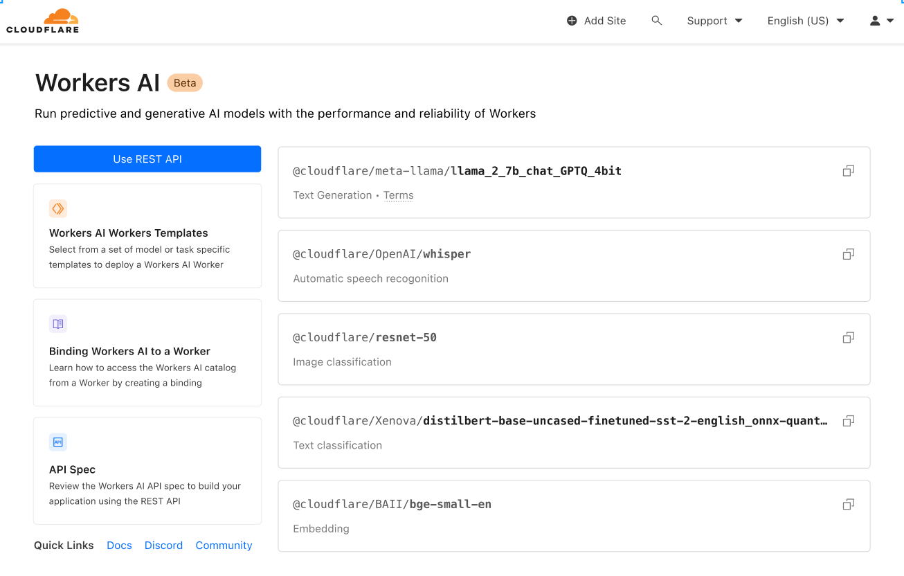
This is just the start, and we’ve got big plans. After launch, we’ll continue to expand based on community feedback. Even more exciting – in an effort to take our catalog from zero to sixty, we’re announcing a partnership with Hugging Face, a leading AI community + hub. The partnership is multifaceted, and you can read more about it here, but soon you’ll be able to browse and run a subset of the Hugging Face catalog directly in Workers AI.
Accessible to everyone
Part of the mission of our developer platform is to provide all the building blocks that developers need to build the applications of their dreams. Having access to the right blocks is just one part of it — as a developer your job is to put them together into an application. Our goal is to make that as easy as possible.
To make sure you could use Workers AI easily regardless of entry point, we wanted to provide access via: Workers or Pages to make it easy to use within the Cloudflare ecosystem, and via REST API if you want to use Workers AI with your current stack.
Here’s a quick CURL example that translates some text from English to French:
curl https://api.cloudflare.com/client/v4/accounts/{ACCOUNT_ID}/ai/run/@cf/meta/@cf/meta/m2m100-1.2b \
-H "Authorization: Bearer {API_TOKEN}" \
	-d '{ "text": "I'll have an order of the moule frites", "target_lang": "french" }'
And here are what the response looks like:
{
  "result": {
    "answer": "Je vais commander des moules frites"
  },
  "success": true,
  "errors":[],
  "messages":[]
}
Use it with any stack, anywhere – your favorite Jamstack framework, Python + Django/Flask, Node.js, Ruby on Rails, the possibilities are endless. And deploy
Designed for developers
Developer experience is really important to us. In fact, most of this post has been about just that. Making sure it works out of the box. Providing popular models that just work. Being accessible to all developers whether you build and deploy with Cloudflare or elsewhere. But it’s more than that – the experience should be frictionless, zero to production should be fast, and it should feel good along the way.
Let’s walk through another example to show just how easy it is to use! We’ll run Llama 2, a popular large language model open sourced by Meta, in a worker.
We’ll assume you have some of the basics already complete (Cloudflare account, Node, NPM, etc.), but if you don’t this guide will get you properly set up!
1. Create a Workers project
Create a new project named workers-ai by running:
$ npm create cloudflare@latest
When setting up your workers-ai worker, answer the setup questions as follows:
- Enter workers-ai for the app name
- Choose Hello World script for the type of application
- Select yes to using TypeScript
- Select yes to using Git
- Select no to deploying
Lastly navigate to your new app directory:
cd workers-ai
2. Connect Workers AI to your worker
Create a Workers AI binding, which allows your worker to access the Workers AI service without having to manage an API key yourself.
To bind Workers AI to your worker, add the following to the end of your wrangler.toml file:
[ai]
binding = "AI" #available in your worker via env.AI
You can also bind Workers AI to a Pages Function. For more information, refer to Functions Bindings.
3. Install the Workers AI client library
npm install @cloudflare/ai --save-dev
4. Run an inference task in your worker
Update the source/index.ts with the following code:
import { Ai } from '@cloudflare/ai'
export default {
  async fetch(request, env) {
    const ai = new Ai(env.AI);
    const input = { prompt: "What's the origin of the phrase 'Hello, World'" };
    const output = await ai.run('@cf/meta/llama-2-7b-chat-int8', input );
    return new Response(JSON.stringify(output));
  },
};
5. Develop locally with Wrangler
While in your project directory, test Workers AI locally by running:
$ npx wranlger dev --remote
Note – These models currently only run on Cloudflare’s network of GPUs (and not locally), so setting `–remote` above is a must, and you’ll be prompted to log in at this point.
Wrangler will give you a URL (most likely localhost:8787). Visit that URL, and you’ll see a response like this
{
  "response": "Hello, World is a common phrase used to test the output of a computer program, particularly in the early stages of programming. The phrase "Hello, World!" is often the first program that a beginner learns to write, and it is included in many programming language tutorials and textbooks as a way to introduce basic programming concepts. The origin of the phrase "Hello, World!" as a programming test is unclear, but it is believed to have originated in the 1970s. One of the earliest known references to the phrase is in a 1976 book called "The C Programming Language" by Brian Kernighan and Dennis Ritchie, which is considered one of the most influential books on the development of the C programming language.
}
6. Deploy your worker
Finally, deploy your worker to make your project accessible on the Internet:
$ npx wranlger dev --remote
# Outputs: https://workers-ai.<YOUR_SUBDOMAIN>.workers.dev
And that’s it. You can literally go from zero to deployed AI in minutes. This is obviously a simple example, but shows how easy it is to run Workers AI from any project.
Privacy by default
When Cloudflare was founded, our value proposition had three pillars: more secure, more reliable, and more performant. Over time, we’ve realized that a better Internet is also a more private Internet, and we want to play a role in building it.
That’s why Workers AI is private by default – we don’t train our models, LLM or otherwise, on your data or conversations, and our models don’t learn from your usage. You can feel confident using Workers AI in both personal and business settings, without having to worry about leaking your data. Other providers only offer this fundamental feature with their enterprise version. With us, it’s built in for everyone.
We’re also excited to support data localization in the future. To make this happen, we have an ambitious GPU rollout plan – we’re launching with seven sites today, roughly 100 by the end of 2023, and nearly everywhere by the end of 2024. Ultimately, this will empower developers to keep delivering killer AI features to their users, while staying compliant with their end users’ data localization requirements.
The power of the platform
Vector database – Vectorize
Workers AI is all about running Inference, and making it really easy to do so, but sometimes inference is only part of the equation. Large language models are trained on a fixed set of data, based on a snapshot at a specific point in the past, and have no context on your business or use case. When you submit a prompt, information specific to you can increase the quality of results, making it more useful and relevant. That’s why we’re also launching Vectorize, our vector database that’s designed to work seamlessly with Workers AI. Here’s a quick overview of how you might use Workers AI + Vectorize together.
Example: Use your data (knowledge base) to provide additional context to an LLM when a user is chatting with it.
- Generate initial embeddings: run your data through Workers AI using an embedding model. The output will be embeddings, which are numerical representations of those words.
- Insert those embeddings into Vectorize: this essentially seeds the vector database with your data, so we can later use it to retrieve embeddings that are similar to your users’ query
- Generate embedding from user question: when a user submits a question to your AI app, first, take that question, and run it through Workers AI using an embedding model.
- Get context from Vectorize: use that embedding to query Vectorize. This should output embeddings that are similar to your user’s question.
- Create context aware prompt: Now take the original text associated with those embeddings, and create a new prompt combining the text from the vector search, along with the original question
- Run prompt: run this prompt through Workers AI using an LLM model to get your final result
AI Gateway
That covers a more advanced use case. On the flip side, if you are running models elsewhere, but want to get more out of the experience, you can run those APIs through our AI gateway to get features like caching, rate-limiting, analytics and logging. These features can be used to protect your end point, monitor and optimize costs, and also help with data loss prevention. Learn more about AI gateway here.
Start building today
Try it out for yourself, and let us know what you think. Today we’re launching Workers AI as an open Beta for all Workers plans – free or paid. That said, it’s super early, so…
Warning – It’s an early beta
Usage is not currently recommended for production apps, and limits + access are subject to change.
Limits
We’re initially launching with limits on a per-model basis
- @cf/meta/llama-2-7b-chat-int8: 5 reqs/min
- All other modes are between 120-180 reqs/min
Checkout our docs for a full overview of our limits.
Pricing
What we released today is just a small preview to give you a taste of what’s coming (we simply couldn’t hold back), but we’re looking forward to putting the full-throttle version of Workers AI in your hands.
We realize that as you approach building something, you want to understand: how much is this going to cost me? Especially with AI costs being so easy to get out of hand. So we wanted to share the upcoming pricing of Workers AI with you.
While we won’t be billing on day one, we are announcing what we expect our pricing will look like.
Users will be able to choose from two ways to run Workers AI:
- Regular Twitch Neurons (RTN) – running wherever there's capacity at $0.01 / 1k neurons
- Fast Twitch Neurons (FTN) – running at nearest user location at $1.25 / 1k neurons
You may be wondering — what’s a neuron?
Neurons are a way to measure AI output that always scales down to zero (if you get no usage, you will be charged for 0 neurons). To give you a sense of what you can accomplish with a thousand neurons, you can: generate 130 LLM responses, 830 image classifications, or 1,250 embeddings.
Our goal is to help our customers pay only for what they use, and choose the pricing that best matches their use case, whether it’s price or latency that is top of mind.
What’s on the roadmap?
Workers AI is just getting started, and we want your feedback to help us make it great. That said, there are some exciting things on the roadmap.
More models, please
We're launching with a solid set of models that just work, but will continue to roll out new models based on your feedback. If there’s a particular model you'd love to see on Workers AI, pop into our Discord and let us know!
In addition to that, we're also announcing a partnership with Hugging Face, and soon you'll be able to access and run a subset of the Hugging Face catalog directly from Workers AI.
Analytics + observability
Up to this point, we’ve been hyper focussed on one thing – making it really easy for any developer to run powerful AI models in just a few lines of code. But that’s only one part of the story. Up next, we’ll be working on some analytics and observability capabilities to give you insights into your usage + performance + spend on a per-model basis, plus the ability to fig into your logs if you want to do some exploring.
A road to global GPU coverage
Our goal is to be the best place to run inference on Region: Earth, so we're adding GPUs to our data centers as fast as we can.
We plan to be in 100 data centers by the end this year

And nearly everywhere by the end of 2024

We’re really excited to see you build – head over to our docs to get started.
If you need inspiration, want to share something you’re building, or have a question – pop into our Developer Discord.
Writing poems using LLama 2 on Workers AI
Post Syndicated from John Graham-Cumming original http://blog.cloudflare.com/writing-poems-using-llama-2-on-workers-ai/


Matthew and Michelle, co-founders of Cloudflare, published their annual founders’ letter today. The letter ends with a poem written by an AI running using Workers AI on Cloudflare’s global network.
Here’s the code that wrote the poem. It uses Workers AI and the Meta Llama 2 model with 7B parameters and 8-bit integers. Just 14 lines of code running on the Cloudflare global network, and you’ve got your very own AI to chat with.
import { Ai } from "@cloudflare/ai";

export default {
    async fetch(request: Request, env: Env): Promise<Response> {
        const body = await request.json();
        const ai = new Ai(env.AI);
        const response = await ai.run("@cf/meta/llama-2-7b-chat-int8", body);
        return new Response(JSON.stringify(response));
    },
};

export interface Env {
    AI: any;
}
That was deployed on Workers AI and all I had to do was ask for poems. Here’s my terminal output (with just the domain name changed).
% curl -X POST https://example.com/ -d '{"prompt":"Write a poem \
that talks about the connectivity cloud"}' | jq -r .response
Cloud computing provides a connectivity that's unmatched,A bridge that spans the globe with ease and grace.It brings us closer, no matter where we are,And makes the world a smaller, more intimate place.
With just a click, we can connect and share,Our thoughts and ideas, our hopes and dreams.The cloud unites us, in a way that's fair,And makes the world a more harmonious theme.
So let us embrace this connectivity,And use it to build a better world for all.For in the cloud, we find a unity,That can help us reach new heights, and stand tall.
% curl -X POST https://example.com/ -d '{"prompt":"Write a poem \
that talks about the connectivity cloud and contrast it with the  \
captivity cloud"}' | jq -r .response
The connectivity cloud, a wondrous sight to see,Where data flows and knowledge is set free,A place where minds meet and ideas take flight,A world of endless possibility in sight.
But then there's the captivity cloud, a darker place,Where thoughts are trapped and minds are in disgrace,A prison of the mind, where freedom's lost,A world of endless sorrow and cost.
So let us choose the connectivity cloud,
And let our minds be free and allowed,
To soar and glide and reach for the sky,
And never be held back, but always fly.
% curl -X POST https://example.com/ -d '{"prompt":"Write a poem \
that talks about the connectivity cloud and contrast it with the  \
captivity cloud using Elizabethan English"}' | jq -r .response
In the connectivity cloud, I find my peace,
Where thoughts and dreams and hopes do cease to flee.
The captivity cloud doth but darken my day,
With chains of sorrow that will not away.
In the connectivity cloud, I find my home,
Where love and joy and laughter do make their moan.
The captivity cloud doth but lock me in,
With sorrow's shackles that will not give in.
In the connectivity cloud, I find my fate,
Where fortune smiles and misery doth wait.
The captivity cloud doth but bring me woe,
With darkness that will not let me go.
In the connectivity cloud, I find my heart,
Where love and hope and joy do play their part.
The captivity cloud doth but tear it apart,
With sorrow's hand that will not let it start.
% curl -X POST https://example.com/ -d '{"prompt":"Write a poem \
that talks about the connectivity cloud and contrast it with the  \
captivity cloud in the style of Lord Byron"}' | jq -r .response
In the realm of the cloud, where data reigns supreme,
A new divide has emerged, a digital dream,
The connectivity cloud, a place of delight,
Where knowledge and wisdom take flight.
But then there's the captivity cloud, a darker hue,
Where privacy and security are hard to pursue,
A prison of sorts, where freedom's light is lost,
And data's secrets are forever crossed.
Yet still, we cling to the captivity cloud,
For in its depths, we find a measure of proof,
That though the connectivity cloud may be bright,
The captivity cloud holds a certain allure in sight.
So let us embrace both, the light and the dark,
For in their union, we find a digital spark,
That illuminates the path to a brighter day,
Where knowledge and privacy reign in a digital way.
What are you going to build on Workers AI? It’s ready and waiting. We’ll help you go from idea to deployed in minutes.
If you want to know exactly how to deploy something like this read the Workers AI announcement blog.
Announcing AI Gateway: making AI applications more observable, reliable, and scalable
Post Syndicated from Michelle Chen original http://blog.cloudflare.com/announcing-ai-gateway/


Today, we’re excited to announce our beta of AI Gateway – the portal to making your AI applications more observable, reliable, and scalable.
AI Gateway sits between your application and the AI APIs that your application makes requests to (like OpenAI) – so that we can cache responses, limit and retry requests, and provide analytics to help you monitor and track usage. AI Gateway handles the things that nearly all AI applications need, saving you engineering time, so you can focus on what you're building.
Connecting your app to AI Gateway
It only takes one line of code for developers to get started with Cloudflare’s AI Gateway. All you need to do is replace the URL in your API calls with your unique AI Gateway endpoint. For example, with OpenAI you would define your baseURL as "https://gateway.ai.cloudflare.com/v1/ACCOUNT_TAG/GATEWAY/openai" instead of "https://api.openai.com/v1" – and that’s it. You can keep your tokens in your code environment, and we’ll log the request through AI Gateway before letting it pass through to the final API with your token.
// configuring AI gateway with the dedicated OpenAI endpoint

const openai = new OpenAI({
  apiKey: env.OPENAI_API_KEY,
  baseURL: "https://gateway.ai.cloudflare.com/v1/ACCOUNT_TAG/GATEWAY/openai",
});
We currently support model providers such as OpenAI, Hugging Face, and Replicate with plans to add more in the future. We support all the various endpoints within providers and also response streaming, so everything should work out-of-the-box once you have the gateway configured. The dedicated endpoint for these providers allows you to connect your apps to AI Gateway by changing one line of code, without touching your original payload structure.
We also have a universal endpoint that you can use if you’d like more flexibility with your requests. With the universal endpoint, you have the ability to define fallback models and handle request retries. For example, let’s say a request was made to OpenAI GPT-3, but the API was down – with the universal endpoint, you could define Hugging Face GPT-2 as your fallback model and the gateway can automatically resend that request to Hugging Face. This is really helpful in improving resiliency for your app in cases where you are noticing unusual errors, getting rate limited, or if one bill is getting costly, and you want to diversify to other models. With the universal endpoint, you’ll just need to tweak your payload to specify the provider and endpoint, so we can properly route requests for you. Check out the example request below and the docs for more details on the universal endpoint schema.
# Using the Universal Endpoint to first try OpenAI, then Hugging Face

curl https://gateway.ai.cloudflare.com/v1/ACCOUNT_TAG/GATEWAY  -X POST \
  --header 'Content-Type: application/json' \
  --data '[
  {
    "provider": "openai",
    "endpoint": "chat/completions",
    "headers": {
      "Authorization": "Bearer $OPENAI_TOKEN",
      "Content-Type": "application/json"
    },
    "query": {
      "model": "gpt-3.5-turbo",
      "stream": true,
      "messages": [
        {
          "role": "user",
          "content": "What is Cloudflare?"
        }
      ]
    }
  },
  {
    "provider": "huggingface",
    "endpoint": "gpt2",
    "headers": {
      "Authorization": "Bearer $HF_TOKEN",
      "Content-Type": "application/json"
    },
    "query": {
      "inputs": "What is Cloudflare?"
    }
  },
]'
Gaining visibility into your app’s usage
Now that your app is connected to Cloudflare, we can help you gather analytics and give insight and control on the traffic that is passing through your apps. Regardless of what model or infrastructure you use in the backend, we can help you log requests and analyze data like the number of requests, number of users, cost of running the app, duration of requests, etc. Although these seem like basic analytics that model providers should expose, it’s surprisingly difficult to get visibility into these metrics with the typical model providers. AI Gateway takes it one step further and lets you aggregate analytics across multiple providers too.
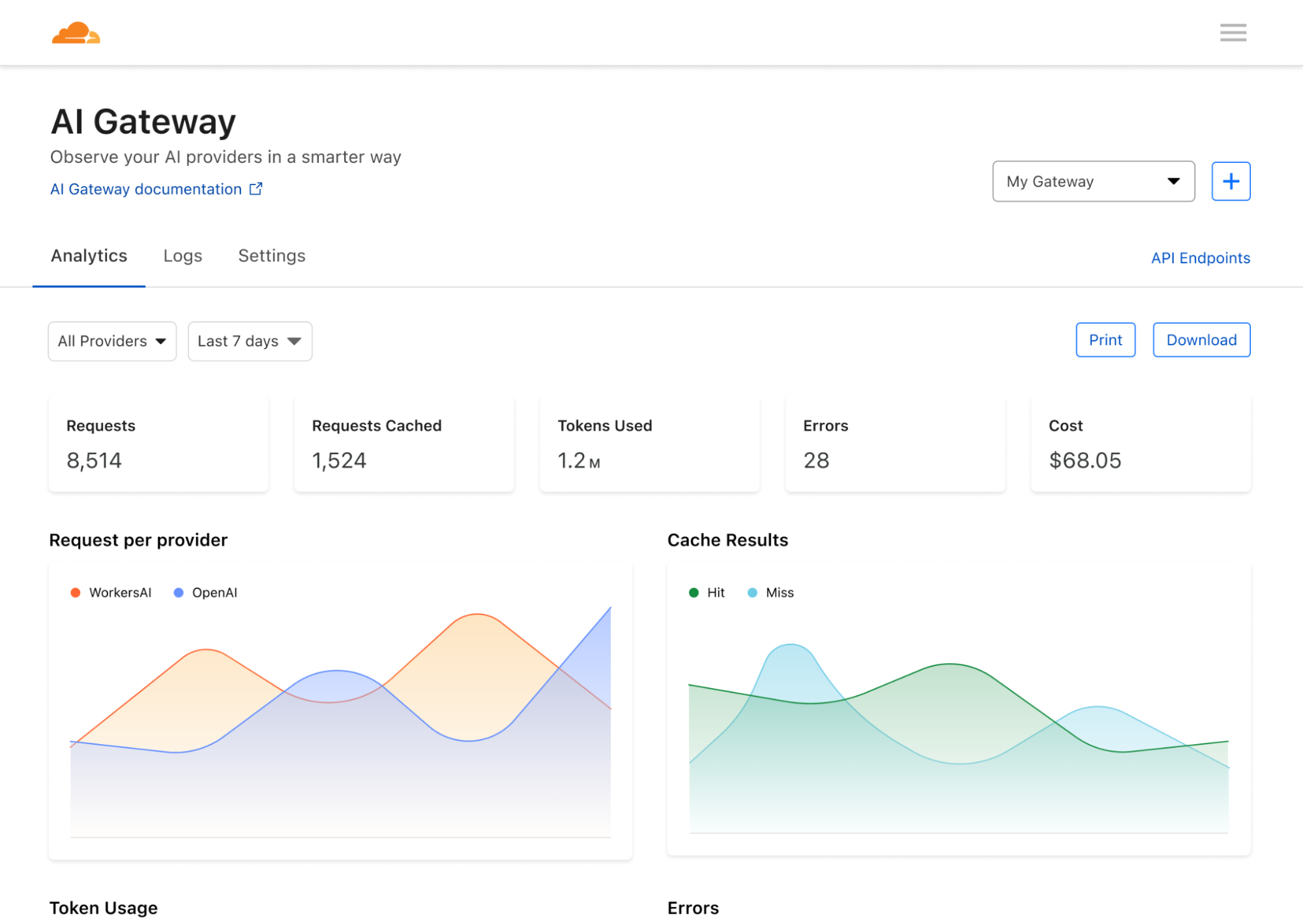
Controlling how your app scales
One of the pain points we often hear is how expensive it costs to build and run AI apps. Each API call can be unpredictably expensive and costs can rack up quickly, preventing developers from scaling their apps to their full potential. At the speed that the industry is moving, you don’t want to be limited by your scale and left behind – and that’s where caching and rate limiting can help. We allow developers to cache their API calls so that new requests can be served from our cache rather than the original API – making it cheaper and faster. Rate limiting can also help control costs by throttling the number of requests and preventing excessive or suspicious activity. Developers have full flexibility to define caching and rate limiting rules, so that apps can scale at a sustainable pace of your choosing.
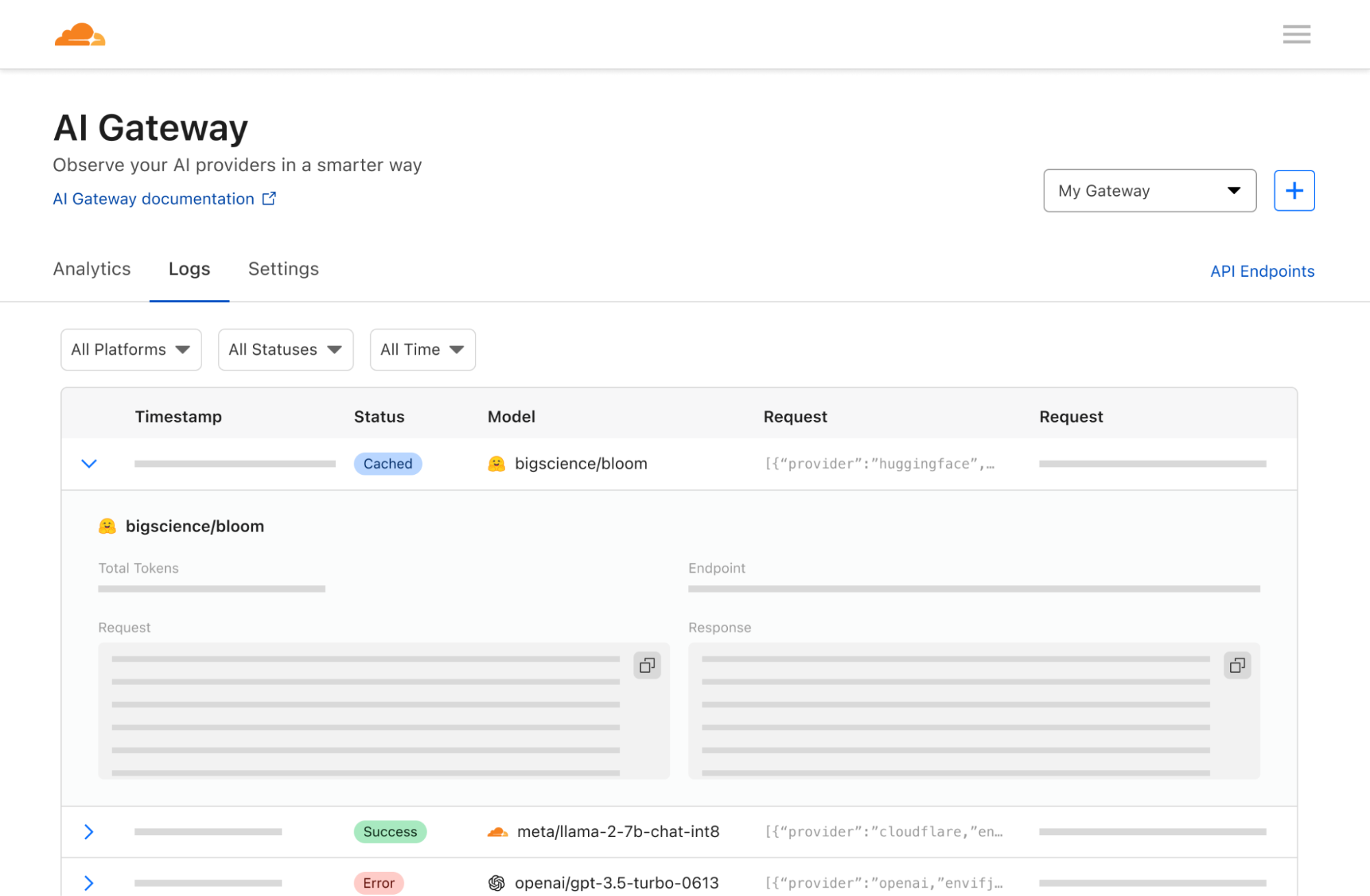
The Workers AI Platform
AI Gateway pairs perfectly with our new Workers AI and Vectorize products, so you can build full-stack AI applications all within the Workers ecosystem. From deploying applications with Workers, running model inference on the edge with Workers AI, storing vector embeddings on Vectorize, to gaining visibility into your applications with AI Gateway – the Workers platform is your one-stop shop to bring your AI applications to life. To learn how to use AI Gateway with Workers AI or the different providers, check out the docs.
Next up: the enterprise use case
We are shipping v1 of AI Gateway with a few core features, but we have plans to expand the product to cover more advanced use cases as well – usage alerts, jailbreak protection, dynamic model routing with A/B testing, and advanced cache rules. But what we’re really excited about are the other ways you can apply AI Gateway…
In the future, we want to develop AI Gateway into a product that helps organizations monitor and observe how their users or employees are using AI. This way, you can flip a switch and have all requests within your network to providers (like OpenAI) pass through Cloudflare first – so that you can log user requests, apply access policies, enable rate limiting and data loss prevention (DLP) strategies. A powerful example: if an employee accidentally pastes an API key to ChatGPT, AI Gateway can be configured to see the outgoing request and redact the API key or block the request entirely, preventing it from ever reaching OpenAI or any end providers. We can also log and alert on suspicious requests, so that organizations can proactively investigate and control certain types of activity. AI Gateway then becomes a really powerful tool for organizations that might be excited about the efficiency that AI unlocks, but hesitant about trusting AI when data privacy and user error are really critical threats. We hope that AI Gateway can alleviate these concerns and make adopting AI tools a lot easier for organizations.
Whether you’re a developer building applications or a company who’s interested in how employees are using AI, our hope is that AI Gateway can help you demystify what’s going on inside your apps – because once you understand how your users are using AI, you can make decisions on how you actually want them to use it. Some of these features are still in development, but we hope this illustrates the power of AI Gateway and our vision for the future.
At Cloudflare, we live and breathe innovation (as you can tell by our Birthday Week announcements!) and the pace of innovation in AI is incredible to witness. We’re thrilled that we can not only help people build and use apps, but actually help accelerate the adoption and development of AI with greater control and visibility. We can’t wait to hear what you build – head to the Cloudflare dashboard to try out AI Gateway and let us know what you think!

Partnering with Hugging Face to make deploying AI easier and more affordable than ever 🤗
Post Syndicated from Rita Kozlov original http://blog.cloudflare.com/partnering-with-hugging-face-deploying-ai-easier-affordable/

Today, we’re excited to announce that we are partnering with Hugging Face to make AI models more accessible and affordable than ever before to developers.
There are three things we look forward to making available to developers over the coming months:
- We’re excited to bring serverless GPU models to Hugging Face — no more wrangling infrastructure or paying for unused capacity. Just pick your model, and go;
- Bringing popular Hugging Face optimized models to Cloudflare’s model catalog;
- Introduce Cloudflare integrations as a part of Hugging Face’s Inference solutions.
Hosting over 500,000 models and serving over one million model downloads a day, Hugging Face is the go-to place for developers to add AI to their applications.
Meanwhile, over the past six years at Cloudflare, our goal has been to make it as easy as possible for developers to bring their ideas and applications to life on our developer platform.
As AI has become a critical part of every application, this partnership has felt like a natural match to put tools in the hands of developers to make deploying AI easy and affordable.
“Hugging Face and Cloudflare both share a deep focus on making the latest AI innovations as accessible and affordable as possible for developers. We’re excited to offer serverless GPU services in partnership with Cloudflare to help developers scale their AI apps from zero to global, with no need to wrangle infrastructure or predict the future needs of your application — just pick your model and deploy.”
— Clem Delangue, CEO of Hugging Face.
We’re excited to share what’s to come, so we wanted to give you a sneak peek into what’s ahead.
Hugging Face models at your fingertips
As a developer, when you have an idea, you want to be able to act on it as quickly as possible. Through our partnership, we’re excited to provide you with familiar models, regardless of where you’re getting started.
If you’re using Cloudflare’s developer platform to build applications, we’re excited to bring Hugging Face models into the flow as a native part of the experience. You will soon be able to deploy Hugging Face models, optimized for performance and speed, right from Cloudflare’s dashboard.
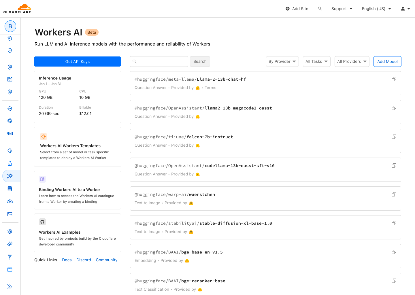
Alternatively, if you’re used to perusing and finding your models on Hugging Face, you will soon be able to deploy them directly from the Hugging Face UI directly to Workers AI.
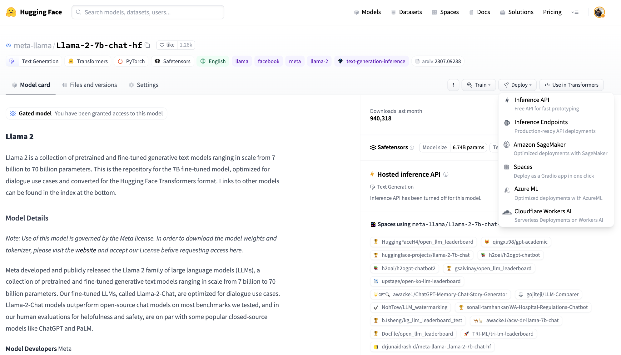
Both of our teams are committed to building the best developer experiences possible, so we look forward to continuing to file away any friction that gets in developers’ ways of building the next big AI idea.
Bringing serverless GPU inference to Hugging Face users
Hugging Face offers multiple inference solutions to serve predictions from the 500,000 models hosted on the platform without managing infrastructure, from the free and rate-limited Inference API, to dedicated infrastructure deployments with Inference Endpoints, and even in-browser edge inference with Transformers.js.
We look forward to working closely with the teams at Hugging Face to enable new experiences powered by Cloudflare: from new serverless GPU inference solutions, to new edge use cases – stay tuned!
See you soon!
We couldn’t wait to share the news with our developers about our partnership, and can’t wait to put these experiences in the hands of developers over the coming months.
Vectorize: a vector database for shipping AI-powered applications to production, fast
Post Syndicated from Matt Silverlock original http://blog.cloudflare.com/vectorize-vector-database-open-beta/

Vectorize is our brand-new vector database offering, designed to let you build full-stack, AI-powered applications entirely on Cloudflare’s global network: and you can start building with it right away. Vectorize is in open beta, and is available to any developer using Cloudflare Workers.
You can use Vectorize with Workers AI to power semantic search, classification, recommendation and anomaly detection use-cases directly with Workers, improve the accuracy and context of answers from LLMs (Large Language Models), and/or bring-your-own embeddings from popular platforms, including OpenAI and Cohere.
Visit Vectorize’s developer documentation to get started, or read on if you want to better understand what vector databases do and how Vectorize is different.
Why do I need a vector database?
Machine learning models can’t remember anything: only what they were trained on.
Vector databases are designed to solve this, by capturing how an ML model represents data — including structured and unstructured text, images and audio — and storing it in a way that allows you to compare against future inputs. This allows us to leverage the power of existing machine-learning models and LLMs (Large Language Models) for content they haven’t been trained on: which, given the tremendous cost of training models, turns out to be extremely powerful.
To better illustrate why a vector database like Vectorize is useful, let’s pretend they don’t exist, and see how painful it is to give context to an ML model or LLM for a semantic search or recommendation task. Our goal is to understand what content is similar to our query and return it: based on our own dataset.
- Our user query comes in: they’re searching for “how to write to R2 from Cloudflare Workers”
- We load up our entire documentation dataset — a thankfully “small” dataset at about 65,000 sentences, or 2.1 GB — and provide it alongside the query from our user. This allows the model to have the context it needs, based on our data.
- We wait.
- (A long time)
- We get our similarity scores back, with the sentences most similar to the user’s query, and then work to map those back to URLs before we return our search results.
… and then another query comes in, and we have to start this all over again.
In practice, this isn’t really possible: we can’t pass that much context in an API call (prompt) to most machine learning models, and even if we could, it’d take tremendous amounts of memory and time to process our dataset over-and-over again.
With a vector database, we don’t have to repeat step 2: we perform it once, or as our dataset updates, and use our vector database to provide a form of long-term memory for our machine learning model. Our workflow looks a little more like this:
- We load up our entire documentation dataset, run it through our model, and store the resulting vector embeddings in our vector database (just once).
- For each user query (and only the query) we ask the same model and retrieve a vector representation.
- We query our vector database with that query vector, which returns the vectors closest to our query vector.
If we looked at these two flows side by side, we can quickly see how inefficient and impractical it is to use our own dataset with an existing model without a vector database:
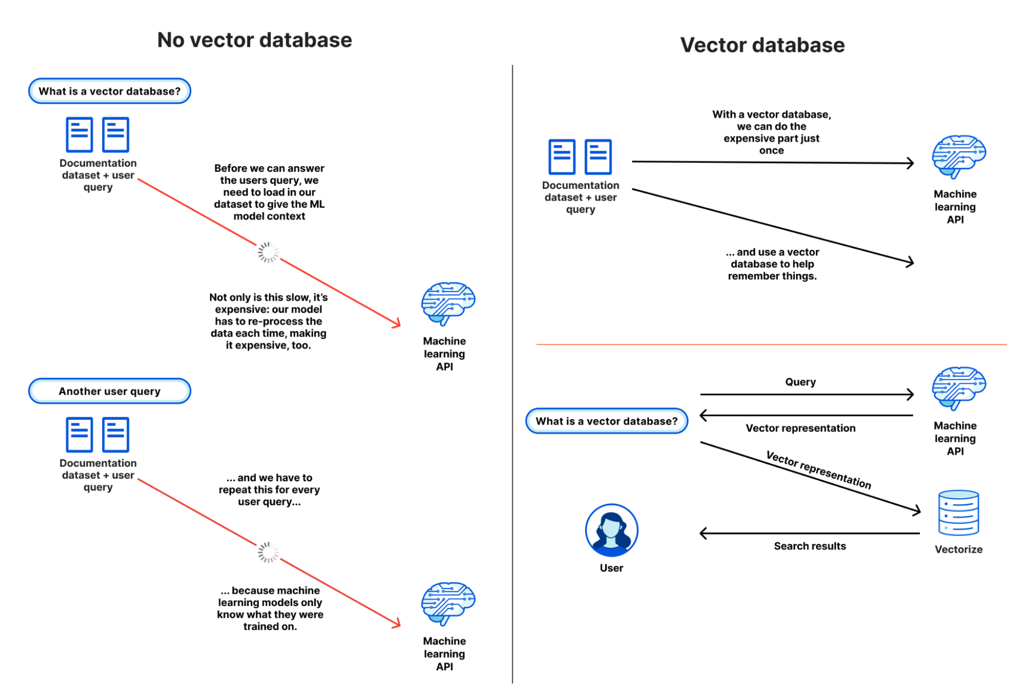
From this simple example, it’s probably starting to make some sense: but you might also be wondering why you need a vector database instead of just a regular database.
Vectors are the model’s representation of an input: how it maps that input to its internal structure, or “features”. Broadly, the more similar vectors are, the more similar the model believes those inputs to be based on how it extracts features from an input.
This is seemingly easy when we look at example vectors of only a handful of dimensions. But with real-world outputs, searching across 10,000 to 250,000 vectors, each potentially 1,536 dimensions wide, is non-trivial. This is where vector databases come in: to make search work at scale, vector databases use a specific class of algorithm, such as k-nearest neighbors (kNN) or other approximate nearest neighbor (ANN) algorithms to determine vector similarity.
And although vector databases are extremely useful when building AI and machine learning powered applications, they’re not only useful in those use-cases: they can be used for a multitude of classification and anomaly detection tasks. Knowing whether a query input is similar — or potentially dissimilar — from other inputs can power content moderation (does this match known-bad content?) and security alerting (have I seen this before?) tasks as well.
Building a recommendation engine with vector search
We built Vectorize to be a powerful partner to Workers AI: enabling you to run vector search tasks as close to users as possible, and without having to think about how to scale it for production.
We’re going to take a real world example — building a (product) recommendation engine for an e-commerce store — and simplify a few things.
Our goal is to show a list of “relevant products” on each product listing page: a perfect use-case for vector search. Our input vectors in the example are placeholders, but in a real world application we would generate them based on product descriptions and/or cart data by passing them through a sentence similarity model (such as Worker’s AI’s text embedding model)
Each vector represents a product across our store, and we associate the URL of the product with it. We could also set the ID of each vector to the product ID: both approaches are valid. Our query — vector search — represents the product description and content for the product user is currently viewing.
Let’s step through what this looks like in code: this example is pulled straight from our developer documentation:
export interface Env {
	// This makes our vector index methods available on env.MY_VECTOR_INDEX.*
	// e.g. env.MY_VECTOR_INDEX.insert() or .query()
	TUTORIAL_INDEX: VectorizeIndex;
}

// Sample vectors: 3 dimensions wide.
//
// Vectors from a machine-learning model are typically ~100 to 1536 dimensions
// wide (or wider still).
const sampleVectors: Array<VectorizeVector> = [
	{ id: '1', values: [32.4, 74.1, 3.2], metadata: { url: '/products/sku/13913913' } },
	{ id: '2', values: [15.1, 19.2, 15.8], metadata: { url: '/products/sku/10148191' } },
	{ id: '3', values: [0.16, 1.2, 3.8], metadata: { url: '/products/sku/97913813' } },
	{ id: '4', values: [75.1, 67.1, 29.9], metadata: { url: '/products/sku/418313' } },
	{ id: '5', values: [58.8, 6.7, 3.4], metadata: { url: '/products/sku/55519183' } },
];

export default {
	async fetch(request: Request, env: Env, ctx: ExecutionContext): Promise<Response> {
		if (new URL(request.url).pathname !== '/') {
			return new Response('', { status: 404 });
		}
		// Insert some sample vectors into our index
		// In a real application, these vectors would be the output of a machine learning (ML) model,
		// such as Workers AI, OpenAI, or Cohere.
		let inserted = await env.TUTORIAL_INDEX.insert(sampleVectors);

		// Log the number of IDs we successfully inserted
		console.info(`inserted ${inserted.count} vectors into the index`);

		// In a real application, we would take a user query - e.g. "durable
		// objects" - and transform it into a vector emebedding first.
		//
		// In our example, we're going to construct a simple vector that should
		// match vector id #5
		let queryVector: Array<number> = [54.8, 5.5, 3.1];

		// Query our index and return the three (topK = 3) most similar vector
		// IDs with their similarity score.
		//
		// By default, vector values are not returned, as in many cases the
		// vectorId and scores are sufficient to map the vector back to the
		// original content it represents.
		let matches = await env.TUTORIAL_INDEX.query(queryVector, { topK: 3, returnVectors: true });

		// We map over our results to find the most similar vector result.
		//
		// Since our index uses the 'cosine' distance metric, scores will range
		// from 1 to -1.  A value of '1' means the vector is the same; the
		// closer to 1, the more similar. Values of -1 (least similar) and 0 (no
		// match).
		// let closestScore = 0;
		// let mostSimilarId = '';
		// matches.matches.map((match) => {
		// 	if (match.score > closestScore) {
		// 		closestScore = match.score;
		// 		mostSimilarId = match.vectorId;
		// 	}
		// });

		return Response.json({
			// This will return the closest vectors: we'll see that the vector
			// with id = 5 has the highest score (closest to 1.0) as the
			// distance between it and our query vector is the smallest.
			// Return the full set of matches so we can see the possible scores.
			matches: matches,
		});
	},
};
The code above is intentionally simple, but illustrates vector search at its core: we insert vectors into our database, and query it for vectors with the smallest distance to our query vector.
Here are the results, with the values included, so we visually observe that our query vector [54.8, 5.5, 3.1] is similar to our highest scoring match: [58.799, 6.699, 3.400] returned from our search. This index uses cosine similarity to calculate the distance between vectors, which means that the closer the score to 1, the more similar a match is to our query vector.
{
  "matches": {
    "count": 3,
    "matches": [
      {
        "score": 0.999909,
        "vectorId": "5",
        "vector": {
          "id": "5",
          "values": [
            58.79999923706055,
            6.699999809265137,
            3.4000000953674316
          ],
          "metadata": {
            "url": "/products/sku/55519183"
          }
        }
      },
      {
        "score": 0.789848,
        "vectorId": "4",
        "vector": {
          "id": "4",
          "values": [
            75.0999984741211,
            67.0999984741211,
            29.899999618530273
          ],
          "metadata": {
            "url": "/products/sku/418313"
          }
        }
      },
      {
        "score": 0.611976,
        "vectorId": "2",
        "vector": {
          "id": "2",
          "values": [
            15.100000381469727,
            19.200000762939453,
            15.800000190734863
          ],
          "metadata": {
            "url": "/products/sku/10148191"
          }
        }
      }
    ]
  }
}
In a real application, we could now quickly return product recommendation URLs based on the most similar products, sorting them by their score (highest to lowest), and increasing the topK value if we want to show more. The metadata stored alongside each vector could also embed a path to an R2 object, a UUID for a row in a D1 database, or a key-value pair from Workers KV.
Workers AI + Vectorize: full stack vector search on Cloudflare
In a real application, we need a machine learning model that can both generate vector embeddings from our original dataset (to seed our database) and quickly turn user queries into vector embeddings too. These need to be from the same model, as each model represents features differently.
Here’s a compact example building an entire end-to-end vector search pipeline on Cloudflare:
import { Ai } from '@cloudflare/ai';
export interface Env {
	TEXT_EMBEDDINGS: VectorizeIndex;
	AI: any;
}
interface EmbeddingResponse {
	shape: number[];
	data: number[][];
}

export default {
	async fetch(request: Request, env: Env, ctx: ExecutionContext): Promise<Response> {
		const ai = new Ai(env.AI);
		let path = new URL(request.url).pathname;
		if (path.startsWith('/favicon')) {
			return new Response('', { status: 404 });
		}

		// We only need to generate vector embeddings just the once (or as our
		// data changes), not on every request
		if (path === '/insert') {
			// In a real-world application, we could read in content from R2 or
			// a SQL database (like D1) and pass it to Workers AI
			const stories = ['This is a story about an orange cloud', 'This is a story about a llama', 'This is a story about a hugging emoji'];
			const modelResp: EmbeddingResponse = await ai.run('@cf/baai/bge-base-en-v1.5', {
				text: stories,
			});

			// We need to convert the vector embeddings into a format Vectorize can accept.
			// Each vector needs an id, a value (the vector) and optional metadata.
			// In a real app, our ID would typicaly be bound to the ID of the source
			// document.
			let vectors: VectorizeVector[] = [];
			let id = 1;
			modelResp.data.forEach((vector) => {
				vectors.push({ id: `${id}`, values: vector });
				id++;
			});

			await env.TEXT_EMBEDDINGS.upsert(vectors);
		}

		// Our query: we expect this to match vector id: 1 in this simple example
		let userQuery = 'orange cloud';
		const queryVector: EmbeddingResponse = await ai.run('@cf/baai/bge-base-en-v1.5', {
			text: [userQuery],
		});

		let matches = await env.TEXT_EMBEDDINGS.query(queryVector.data[0], { topK: 1 });
		return Response.json({
			// We expect vector id: 1 to be our top match with a score of
			// ~0.896888444
			// We are using a cosine distance metric, where the closer to one,
			// the more similar.
			matches: matches,
		});
	},
};
The code above does four things:
- It passes the three sentences to Workers AI’s text embedding model (
@cf/baai/bge-base-en-v1.5) and retrieves their vector embeddings. - It inserts those vectors into our Vectorize index.
- Takes the user query and transforms it into a vector embedding via the same Workers AI model.
- Queries our Vectorize index for matches.
This example might look “too” simple, but in a production application, we’d only have to change two things: just insert our vectors once (or periodically via Cron Triggers), and replace our three example sentences with real data stored in R2, a D1 database, or another storage provider.
In fact, this is incredibly similar to how we run Cursor, the AI assistant that can answer questions about Cloudflare Worker: we migrated Cursor to run on Workers AI and Vectorize. We generate text embeddings from our developer documentation using its built-in text embedding model, insert them into a Vectorize index, and transform user queries on the fly via that same model.
BYO embeddings from your favorite AI API
Vectorize isn’t just limited to Workers AI, though: it’s a fully-fledged, standalone vector database.
If you’re already using OpenAI’s Embedding API, Cohere’s multilingual model, or any other embedding API, then you can easily bring-your-own (BYO) vectors to Vectorize.
It works just the same: generate your embeddings, insert them into Vectorize, and pass your queries through the model before you query your index. Vectorize includes a few shortcuts for some of the most popular embedding models.
# Vectorize has ready-to-go presets that set the dimensions and distance metric for popular embeddings models
$ wrangler vectorize create openai-index-example --preset=openai-text-embedding-ada-002
This can be particularly useful if you already have an existing workflow around an existing embeddings API, and/or have validated a specific multimodal or multilingual embeddings model for your use-case.
Making the cost of AI predictable
There’s a tremendous amount of excitement around AI and ML, but there’s also one big concern: that it’s too expensive to experiment with, and hard to predict at scale.
With Vectorize, we wanted to bring a simpler pricing model to vector databases. Have an idea for a proof-of-concept at work? That should fit into our free-tier limits. Scaling up and optimizing your embedding dimensions for performance vs. accuracy? It shouldn’t break the bank.
Importantly, Vectorize aims to be predictable: you don’t need to estimate CPU and memory consumption, which can be hard when you’re just starting out, and made even harder when trying to plan for your peak vs. off-peak hours in production for a brand new use-case. Instead, you’re charged based on the total number of vector dimensions you store, and the number of queries against them each month. It’s our job to take care of scaling up to meet your query patterns.
Here’s the pricing for Vectorize — and if you have a Workers paid plan now, Vectorize is entirely free to use until 2024:
| Workers Free (coming soon) | Workers Paid ($5/month) | |
|---|---|---|
| Queried vector dimensions included | 30M total queried dimensions / month | 50M total queried dimensions / month |
| Stored vector dimensions included | 5M stored dimensions / month | 10M stored dimensions / month |
| Additional cost | $0.04 / 1M vector dimensions queried or stored | $0.04 / 1M vector dimensions queried or stored |
Pricing is based entirely on what you store and query: (total vector dimensions queried + stored) * dimensions_per_vector * price. Query more? Easy to predict. Optimizing for smaller dimensions per vector to improve speed and reduce overall latency? Cost goes down. Have a few indexes for prototyping or experimenting with new use-cases? We don’t charge per-index.
As an example: if you load 10,000 Workers AI vectors (384 dimensions each) and make 5,000 queries against your index each day, it’d result in 49 million total vector dimensions queried and still fit into what we include in the Workers Paid plan ($5/month). Better still: we don’t delete your indexes due to inactivity.
Note that while this pricing isn’t final, we expect few changes going forward. We want to avoid the element of surprise: there’s nothing worse than starting to build on a platform and realizing the pricing is untenable after you’ve invested the time writing code, tests and learning the nuances of a technology.
Vectorize!
Every Workers developer on a paid plan can start using Vectorize immediately: the open beta is available right now, and you can visit our developer documentation to get started.
This is also just the beginning of the vector database story for us at Cloudflare. Over the next few weeks and months, we intend to land a new query engine that should further improve query performance, support even larger indexes, introduce sub-index filtering capabilities, increased metadata limits, and per-index analytics.
If you’re looking for inspiration on what to build, see the semantic search tutorial that combines Workers AI and Vectorize for document search, running entirely on Cloudflare. Or an example of how to combine OpenAI and Vectorize to give an LLM more context and dramatically improve the accuracy of its answers.
And if you have questions about how to use Vectorize for our product & engineering teams, or just want to bounce an idea off of other developers building on Workers AI, join the #vectorize and #workers-ai channels on our Developer Discord.