Post Syndicated from Sprites mods original https://spritesmods.com/?art=vapourdeck&f=rss
I always wanted to build my own 486 PC, so I built one, and put it into a form factor that’s quite unique for a retro-machine
Post Syndicated from Sprites mods original https://spritesmods.com/?art=vapourdeck&f=rss
I always wanted to build my own 486 PC, so I built one, and put it into a form factor that’s quite unique for a retro-machine
Post Syndicated from jzb original https://lwn.net/Articles/1080188/
Git maintainer Junio Hamano has announced
Git 2.55.0, which has non-merge commits from 100 people; 33 of
those are first-time contributors to the project. LWN recently covered some of
the noteworthy changes in 2.55, including new features for the
experimental “git history” command, addition of the Git fsmonitor
daemon for Linux systems, and more.
Post Syndicated from Raza Hafeez original https://aws.amazon.com/blogs/big-data/scale-analytics-with-amazon-redshift-multi-warehouse-enhancements/
Onboard analytics workloads at scale with Amazon Redshift’s improved remote table data definition language (DDL), materialized view improvements, and concurrency scaling enhancements for zero-ETL and auto-copy.
As organizations scale their analytics capabilities, they need the ability to add workloads without disrupting production operation or being constrained by the resources of a single data warehouse. In this post, we introduce new capabilities of Amazon Redshift that enhance our multi-warehouse and scaling capabilities: remote materialized view (MV) operations, remote table DDL support, and concurrency scaling enhancements for zero-ETL and S3 event integration. These features help you build more scalable, performant decentralized analytics architectures on Amazon Redshift.
Let us review how these new features enable you to run analytics at scale.
ALTER TABLE ALTER DISTSTYLE operations now work on remote warehouses through concurrency scaling and data sharing. You can dynamically optimize data distribution across distributed environments, improving query performance and resource utilization without requiring data migration. This is especially valuable for data engineers fine-tuning performance across multiple warehouses and administrators adapting to changing query patterns.ALTER TABLE APPEND operations now extend to remote warehouses through concurrency scaling and data sharing. This consolidates data across distributed environments, so you can efficiently combine tables without complex data movement or extract, transform, and load (ETL) processes. Organizations managing dynamic table operations across multiple environments can maintain data consistency while reducing operational overhead.With these new concurrency scaling capabilities, you can maintain consistent data freshness without compromising existing warehouse performance. This eliminates the traditional trade-off between analytics and data loading. Apart from turning on concurrency scaling, no additional changes are required to take advantage of these features.
This section covers two industry use cases: the first for a financial services customer and the second for a gaming industry customer.
The following is a sample architecture for a large financial services customer with global operations. This customer uses a multi-warehouse architecture built on Amazon Redshift.
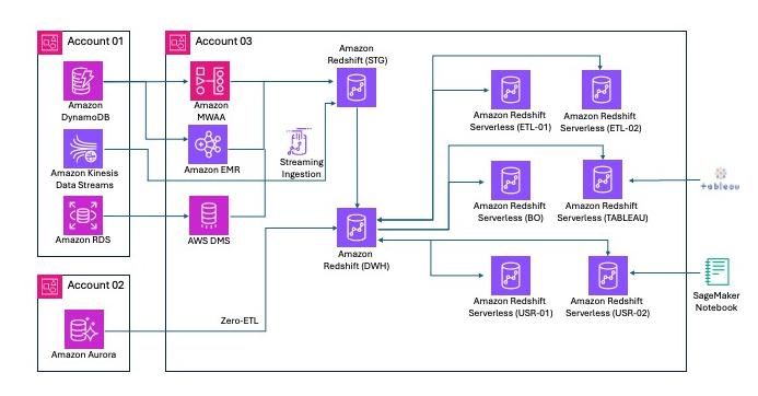
The staging (STG) warehouse serves as a raw zone for data from various sources, like the bronze layer of a medallion architecture. This warehouse also cleanses and standardizes the raw data to the silver layer and makes it available for further processing. The STG warehouse uses MVs to process millions of nested JSON messages and extract attributes into scalar columnar Amazon Redshift tables.
The DWH warehouse serves as the primary Amazon Redshift instance and gold layer, providing data to consuming applications like Business Objects and Tableau. The zero-ETL concurrency scaling improvements provide consistent data freshness even when zero-ETL ingestion spikes occur alongside heavy DWH workloads. The DWH MVs provide fast access to aggregated data for Tableau extracts and Business Objects live reports. The DWH warehouse takes advantage of concurrency scaling when multiple MVs need to be refreshed on the DWH instance.
The ETL01/02 warehouses serve as dedicated compute environments for running project-specific ETL jobs, while the USR01/02 warehouses handle user workloads such as ad-hoc analysis or model building from dbt. When new objects are required by user workloads, they are created and maintained on the remote producer warehouse (DWH).
A leading gaming company has built their entire analytics infrastructure on AWS, with their analytics team managing data streaming from games, data warehousing, and business intelligence tools. They standardized Amazon Redshift across the organization, migrating off Vertica running on Amazon Elastic Compute Cloud (Amazon EC2). After overcoming early challenges with cluster resize operations, the team became strong advocates for Amazon Redshift and now runs their primary production cluster on 32 ra3.16xlarge nodes.
As their data ingestion pipeline grew, query workloads began competing with data ingestion processes, creating performance bottlenecks. Rather than scaling up their primary cluster, they implemented a workload isolation strategy using Amazon Redshift data sharing. The customer launched a second 16-node ra3.4xlarge cluster as a data share consumer, with the primary cluster serving as the producer. This architecture allowed them to migrate consumption workloads to the consumer cluster while the producer focused on data ingestion, effectively supporting growth without increasing the primary cluster size.
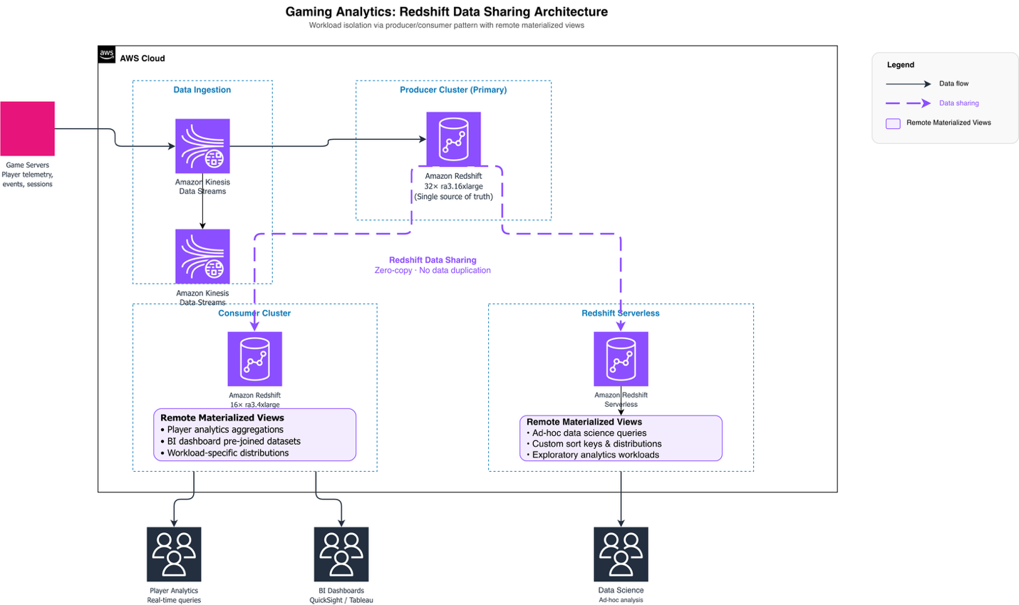
Recognizing the advantages of this distributed architecture, the gaming company expanded their approach by migrating workloads to Amazon Redshift Serverless, further using the data sharing model for workload isolation. Amazon Redshift’s remote materialized view capability allowed the gaming company to create materialized views directly on the data shared by the producer cluster. Each consumer cluster could now build materialized views optimized for its specific workload patterns. This created pre-aggregated datasets, custom join strategies, and workload-specific data distributions, without impacting the producer cluster’s performance or requiring data duplication. The producer warehouse maintains data distribution and sorting strategies designed for generic enterprise needs, providing consistent data quality across all consumers. Meanwhile, consumer warehouses used remote materialized views to fine-tune query performance for their distinct analytical requirements, whether supporting real-time player analytics, business intelligence dashboards, or ad-hoc data science workloads. This distributed approach to data consumption optimization proved essential for the gaming company. It delivered fast query performance across diverse analytical workloads while maintaining a single source of truth in the producer cluster and avoiding the operational overhead of managing redundant data copies.
To get the most out of these new capabilities, consider the following best practices:
MaxRPU setting. This helps you avoid unexpected additional costs. For more information, see the Amazon Redshift usage limits documentation.In this post, we walked through the new MV refresh features, remote table DDL capabilities, and expanded concurrency scaling support for zero-ETL and S3 auto-copy. These features help you move beyond the constraints of a single warehouse. They are particularly valuable for organizations managing distributed data architectures that require dynamic table management across multiple environments while maintaining data consistency and adapting quickly to changing workloads. To get started, make sure you are running the latest Amazon Redshift version. Then visit the Amazon Redshift documentation to learn more about concurrency scaling, data sharing, and materialized views.
Post Syndicated from Shannon Brazil original https://aws.amazon.com/blogs/security/what-the-june-2026-threat-technique-catalog-update-means-for-your-aws-environment/
The AWS Customer Incident Response Team (AWS CIRT) encounters patterns that repeat across engagements when helping customers respond to security incidents. We’re passionate about making sure that information is accessible so that everyone can improve their security posture and their organization’s resilience to disruption. The primary method we use to share this information is the Threat Technique Catalog for AWS (TTC). The latest update to the catalog for June 2026 focuses on container security, organization-level trust, and compute hijacking. Each new entry reflects something we’ve encountered in practice, and each provides straightforward mitigation. This post breaks down what changed, why it matters, and what you can do about it today.
We’ve added five new entries to the TTC.
Amazon Elastic Kubernetes Service (Amazon EKS) gives teams powerful orchestration capabilities. We’re seeing threat actors who have obtained Kubernetes credentials or an AWS Identity and Access Management (IAM) role with EKS permissions modify running workloads—altering container images, injecting sidecar containers, or changing pod specifications to introduce malicious code into a deployment.
Nothing new is created. The workload already exists, it might be running in production, and by modifying it in place the threat actor inherits the network access, service account permissions, and data access the legitimate workload already had. Without admission controllers or image verification, these changes can go unnoticed until the impact shows up downstream. Enforcing image signing through admission controllers, restricting workload changes with Kubernetes role-based access control (RBAC), and enabling Amazon GuardDuty EKS Protection to surface anomalous cluster activity all reduce this risk. For more information, see EKS Modification – Workload Integrity Degradation.
Publicly exposed Kubernetes API servers and misconfigured ingress controllers continue to be an entry point we see exploited. This technique captures threat actors targeting the customer-deployed workloads running on Amazon EKS—not EKS itself—and their exposure to the internet.
The pattern starts with an exposed service and an application-level weakness, then pivots from the compromised pod toward broader cluster access. When inside a pod, a threat actor can query the instance metadata service, read mounted service account tokens, or move laterally across the cluster network. Limiting public exposure of the Kubernetes API server, applying network policies to restrict pod-to-pod communication, and running workloads with least-privilege service accounts reduce the risk of this technique succeeding. For more information about this technique, see Exploit Public-Facing Application.
AWS Organizations centralizes trust across member accounts, and that trust runs in one direction—from the management account downward. We’ve observed threat actors who compromise a management account—or gain sufficient privilege within one—use that position to assume root access into member accounts using sts:AssumeRoot. Because the trust is inherent to the organization structure, this can avoid the access controls a member account administrator has configured.
With root access to a member account, a threat actor can disable security controls, delete resources, change billing configurations, and establish persistence that survives remediation focused on IAM principals. We strongly encourage implementing service control policies (SCPs) that restrict which principals can call sts:AssumeRoot and under what conditions, and monitoring for sts:AssumeRoot calls in AWS CloudTrail. For more information, see Assume Root into Organization Member Account.
Compute hijacking remains one of the most common motivations we see behind unauthorized access, and Amazon EKS clusters are increasingly the target. Threat actors deploy cryptocurrency mining or other compute-intensive workloads inside compromised clusters, consuming customer resources and generating unexpected cost.
What sets EKS-based hijacking apart is scale. In clusters without resource quotas, a single compromised service account can consume all available capacity across nodes. The workloads use legitimate-looking images pulled from public registries, which makes image scanning alone insufficient. Setting resource quotas and limit ranges, restricting which registries workloads can pull from, and enabling Amazon GuardDuty EKS Protection to flag mining behavior provides effective detection. For more information, see Resource Hijacking: Compute Hijacking – EKS.
A threat actor with access to a standalone account—or one they’ve removed from its legitimate organization—invites it into an organization they control. After the account joins, it falls under the threat actor’s governance. The threat actor’s organization can apply SCPs that restrict the legitimate owner’s actions, gain visibility into the account’s resources through organizational services, and access consolidated billing information. The legitimate owner finds themselves locked out of their own governance controls. Monitoring organizations:InviteAccountToOrganization and organizations:AcceptHandshake, and implementing SCPs that prevent accounts from leaving their legitimate organization are important preventive measures. For more information, see Modify Cloud Resource Hierarchy: Invite Accounts to Unknown Organization.
We’ve refreshed three existing entries. S3 Object Collection now captures additional API calls used for bulk data staging from Amazon Simple Storage Service (Amazon S3), with refined detection guidance and mitigations that use recent Amazon S3 security features. Compute Hijacking – ECS adds methods threat actors use to deploy unauthorized tasks in Amazon Elastic Container Service (Amazon ECS), including abuse of overly permissive task execution roles. Role Assumption and Federated Access has been expanded to cover new cross-account role assumption variations and identity provider manipulation, with sharper guidance for distinguishing legitimate federated access from unauthorized use.
This June update reflects a clear trend: threat actors are increasingly targeting container orchestration platforms and using organizational trust relationships to their advantage. The container techniques show that as organizations adopt Kubernetes at scale, the attack surface grows with it. The organization-level techniques show that threat actors understand organizational trust relationships.
The common thread is that every one of these techniques operates within the boundaries of legitimate functionality. Modifying a workload, assuming cross-account trust, and joining an organization are all expected actions in healthy environments.. Detection, then, depends entirely on context: the principal, the timing, and the sequence of events that follows.
The Threat Technique Catalog for AWS is designed to help with this. We encourage teams to review the relevant entries and assess whether their current monitoring would catch these patterns:
sts:AssumeRoot calls into member accountsEach of the threats leaves traces in AWS CloudTrail and Kubernetes audit logs, and the TTC provides specific guidance on what to watch for and how to respond.
The Threat Technique Catalog for AWS exists because we believe the patterns we observe during security engagements shouldn’t stay behind closed doors. When we see techniques repeating across customers, the most effective thing we can do is document them and make that knowledge available so you can act on it before you’re in the middle of an incident.
This June update adds five new entries and updates three existing ones, and the catalog will continue to evolve. Our team updates it based on what we’re seeing in the real world when helping customers respond to security events. We encourage security teams to review the catalog, incorporate its techniques into threat modeling exercises, and use it as a shared vocabulary for discussing cloud-specific threats.
Explore the full catalog: Threat Technique Catalog for AWS – Full Matrix
If you have feedback about this post, submit comments in the Comments section below.
Post Syndicated from Patrick Kennedy original https://www.servethehome.com/amd-epyc-8005-sorano-completely-changes-amd-sp6/
We take a look at the AMD EPYC 8005 “Sorano” and see one of the biggest generational upheavals in server CPUs we have seen since 2019
The post AMD EPYC 8005 Sorano Completely Changes AMD SP6 appeared first on ServeTheHome.
Post Syndicated from Ben Freiberg original https://aws.amazon.com/blogs/architecture/lessons-learned-from-scaling-to-1-million-lambda-functions/
In this post, we share our journey and the lessons learned from building and running a fully serverless, multi-account software as a service (SaaS) platform at scale. We’ll explore why true scale-to-zero is critical, how we handle quota management, why engaging AWS service teams early saved us from outages, and which unexpected practices emerged once we scaled from thousands to over a million functions.
At ProGlove, we build smart wearable barcode scanning solutions that connect frontline workers to digital workflows. Our scanners integrate with Insight, our AWS-based SaaS platform, to provide real-time visibility into processes, helping customers in manufacturing, logistics and retail improve productivity, reduce errors and enhance ergonomics on the shop floor.
We chose a one AWS account per tenant architecture to achieve clearer security boundaries, streamlined ownership of services, and more transparent cost. It is important to focus on efficiency with dedicated tenant resources at scale, because resource wastage will also scale. The ability to scale-to-zero removes this concern.
When you first build a serverless system, you think in single digits. A handful of AWS Lambda functions, maybe a few dozen at most. It’s hard to imagine what changes when your platform operates thousands of AWS accounts and deploys over one million Lambda functions into production, each isolated to a single customer’s account.
We followed standard playbooks, where “scale-to-zero” was merely a nice-to-have. We used serverless best practices like Amazon Simple Queue Service (Amazon SQS) for decoupling and long-polling to keep the application responsive and resilient. At this scale, a few idle functions or a handful of accounts were a negligible expense and the benefits of a high-level managed service like AWS Lambda really showed.
Each microservice in our platform follows a consistent structure: 5 to 15 Lambda functions coordinated by AWS Step Functions, with Amazon EventBridge handling event routing and Amazon DynamoDB as the primary data store.
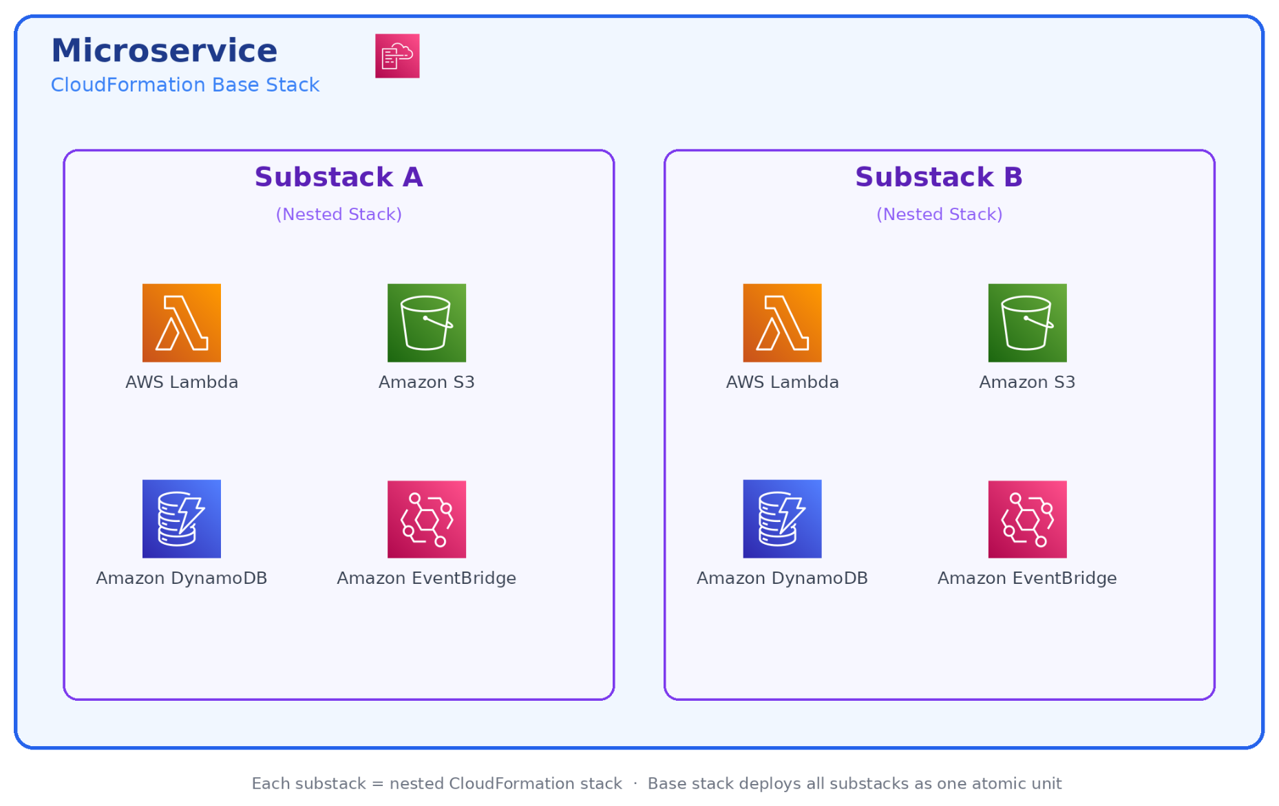
These resources are bundled together into a dedicated AWS CloudFormation stack for deployment.
As we onboarded our first handful of tenants, it quickly became clear that deploying and updating AWS CloudFormation stacks individually per account wouldn’t scale. We adopted AWS CloudFormation StackSets, which let us push infrastructure updates to multiple accounts in parallel from a central management account. At this stage, StackSets felt like a superpower. One deployment operation and many accounts are updated simultaneously. We evaluated building a fully custom replacement later, but ultimately concluded that the maintenance overhead wasn’t worth the marginal control gains and stayed with StackSets as our core mechanism.
Growing to 50 tenant accounts forced us to confront problems that weren’t visible at single-digit scale. Three areas in particular required deliberate architectural decisions: observability, account provisioning, and quota isolation.
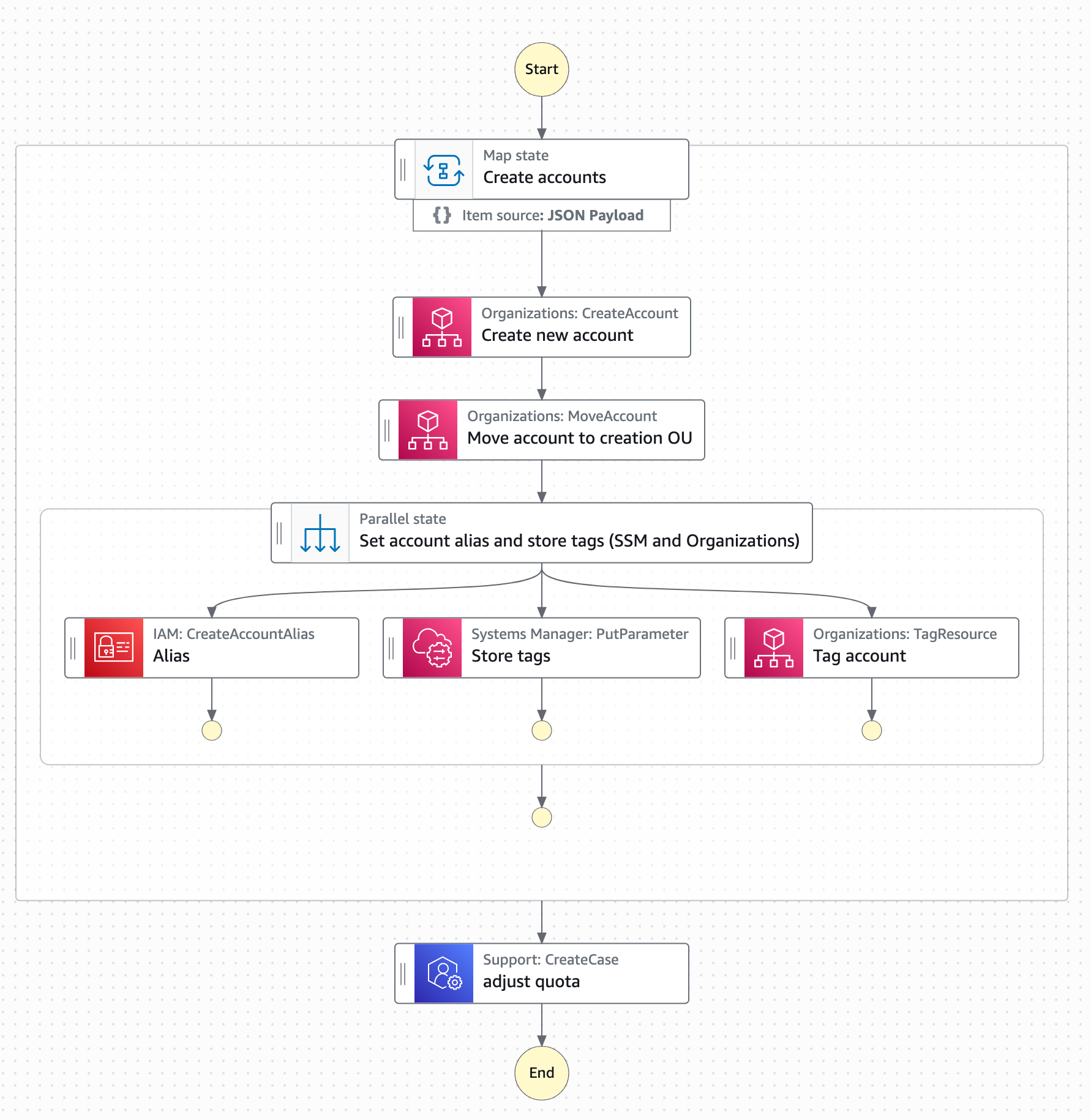
We knew manual provisioning would not scale. Instead we built an automated account factory on top of AWS Organizations: an AWS Step Functions workflow in the management account handles the full provisioning lifecycle: Creating the account, applying baseline service control policies (SCPs), bootstrapping cross-account IAM roles, and triggering the initial CloudFormation StackSet deployment. All done using cross-account AWS Lambda invocations. New tenant accounts go from request to ready in under 15 minutes, at near-zero incremental cost per provisioning run.
One underappreciated advantage of the account-per-tenant model is quota separation. Each account gets its own Lambda concurrent execution limit, its own Amazon API Gateway throttle, and its own service quotas across the board. In a shared-account SaaS model at this scale, a single noisy tenant could exhaust shared concurrency and cause cascading failures across all other tenants. With account isolation, that class of problem simply doesn’t exist as each tenant’s activity is bound to their own account.
As our fleet grew beyond a few hundred accounts, we began to experience the “Physics of Scale”. We discovered that when hundreds of backend service instances simultaneously access other services, the resulting request volume can resemble a coordinated attack, impacting not only our own infrastructure but also AWS.
One time, we faced a massive metric spike where our own functions effectively overwhelmed (similar to a DDoS attack) our internal APIs. The root cause was synchronized schedules: every Lambda was using the same rate(5 minutes) expression, which aligned to the top of the minute across thousands of accounts.
The solution was request scattering. We now use a standardized internal library that enforces jitter, randomized batch offsets, and staggered updates across all scheduled functions.
Rule of Thumb: “Never do the same thing at the same time everywhere”.
With several dozen accounts, manual log access per account became unworkable. We adopted a third-party observability platform, forwarding Amazon CloudWatch logs and metrics cross-account to a centralized dashboard. At roughly $3 per account per month, the cost felt insignificant.
That assumption was soon replaced by a very real learning: at thousands of accounts, $3 per account per month becomes an impactful expense that demands active management. We learned to treat per-account observability costs with the same scrutiny you apply to compute costs.
What came as a surprise to us were the actual cost drivers: instead of Lambda compute or storage costs, we found that forwarding all observability data almost doubled our cloud bill. As a result, we had to learn how to differentiate between high and low priority observability data and only move around the priority data.
With all mitigations combined we managed to bring observability costs down to around $0.7 per account. Additionally, we were able to switch accounts to almost 0 after some time of inactivity by only monitoring a small set of very basic metrics.
One of the most painful lessons was realizing that traditional Amazon SQS “best practices” increased costs in our use-case and scale.
After we scaled to over a thousand AWS accounts, we understood that “idle” doesn’t necessarily mean there are no costs – even when using Serverless. When Lambda functions consume events from EventBridge through an SQS queue to increase resilience, they constantly make requests to the queue even when there are no messages to process.
To eliminate the cost of continuous polling, we removed Amazon SQS from the path between Amazon EventBridge and AWS Lambda.
AsyncEventsDropped and ConcurrentExecutions to make sure we stay within our quotas without losing events.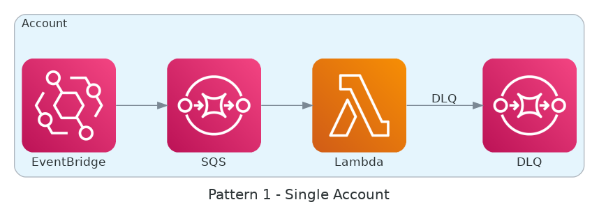
Individual DLQ per queue
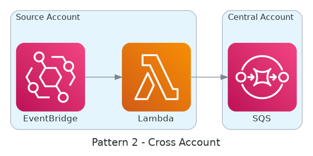
Centralized DLQ polling
Serverless architectures grow to large numbers of infrastructure components: where a monolith or Amazon Elastic Compute Cloud (Amazon EC2)-based service might be a handful of resources, a single microservice in our stack spans dozens of Lambda functions, EventBridge rules, DynamoDB tables, and Step Functions state machines. Multiplied across thousands of accounts, deployment complexity compounds quickly.
Initially, we used AWS CloudFormation StackSets to roll out updates in parallel. However, at the scale of 1 million Lambda functions, StackSets hit a performance ceiling and occasionally produced errors that added up significantly at our volume.
The bottlenecks became such a blocker that we began building our own internal serverless deployment system to replace StackSets. This caught the attention of the AWS CloudFormation service team, who committed to supporting our use case at the scale we required and partnered with us closely from that point on.
By engaging early and often, we were able to:
Being able to scale a serverless platform with a small team of engineers requires consistent and efficient governance practices. This applies to both cloud governance topics as well as engineering practices. Otherwise it will be next to impossible to keep software delivery and development performance as well as reliability at a high level over time.
Cost optimization also changes at a higher maturity level: once cost control is tightly monitored and automated, the discipline changes from housekeeping tasks to collect easy cost savings towards increasingly complex architectural changes. For example, if a new feature significantly increases the number of Lambda invocations and drives up cost, you will need to re-think the architecture and include the new focus on cost.
We consolidated 20 microservices into a single mono-repo. This helped us to:
Even with a scale-to-zero mandate, we learned that “zero” is often “almost-zero”.
One of the most valuable habits we built was resisting the urge to immediately default to a familiar pattern or write custom code. AWS offers a growing catalog of fully managed, event-driven services such as Amazon EventBridge Pipes, AWS AppSync, Amazon SQS FIFO, and others, that can remove entire categories of custom Lambda code. Before writing a function, ask whether a native service integration already solves the problem.
A deliberate research step of exploring native AWS capabilities before opening an editor consistently paid off. It reduces the surface area you own, eliminates maintenance burden, and builds the team’s instinct for choosing the right service over reinventing it. Serverlessland is an excellent starting point for discovering patterns and service combinations you may not have considered.
Scaling from 0 to 1M Lambda functions across thousands of AWS accounts is a question of efficiency not of capacity. Every new account, every new customer, adds potential operational load. The only way to stay ahead is to make sure efficiency scales faster than growth. For us, that means true scale-to-zero, proactive and efficient quota management, tight collaboration with AWS service teams, disciplined developer education, and a mono-repo that enforces consistency.
We’ve learned that the difference between success and failure at this scale lies in unexpected aspects like the hard-learned fact that observability becomes an increasingly complex problem the more distributed your platform becomes.
The benefits are substantial. With the right automation and architectural rigor, a lean team can operate a large-scale infrastructure. Using a cloud-native approach based on serverless services is the most important operational advantage in this case.
To apply these lessons to your own workloads, discover event-driven patterns and service combinations on Serverless Land.
Post Syndicated from Ajish Abraham original https://aws.amazon.com/blogs/architecture/preventing-data-exfiltration-in-machine-learning-environments-with-amazon-sagemaker-ai/
If you’re building machine learning solutions with sensitive data, you face a persistent challenge: preventing data exfiltration while enabling data scientists to work productively. iBusiness, an AI-driven fintech organization, needed its data scientists to work with sensitive data to fine-tune and improve machine learning models. As the data science team scaled, traditional air-gapped environments and monitored virtual desktops proved unsustainable, leading to high costs and operational complexity.
In this post, we demonstrate how iBusiness implemented a three-layered security architecture using Amazon SageMaker AI, virtual private cloud (VPC) endpoints, and Amazon WorkSpaces Secure Browser to prevent data exfiltration while maintaining data scientist productivity. You can adapt this approach to build secure machine learning environments that balance strict data protection with team scalability.
Historically, when access to sensitive data was required, iBusiness provided an isolated, air-gapped on-premises environment. However, with the shift to a remote workforce, this approach became impractical. The company locked down secure virtual desktops through device management policies and had them monitored by proctors to prevent inappropriate actions.
As the data science team scaled and expanded machine learning (ML) use cases, this approach proved unsustainable. Each user required a dedicated virtual desktop, even for temporary access, leading to increased costs. Additionally, maintaining ML tools, libraries, and patches in these locked-down environments was time-consuming and operationally complex.
To address these challenges, iBusiness adopted Amazon SageMaker Studio, a fully managed, web-based ML development environment. This removed the need to maintain in-house Jupyter environments while giving data scientists access to up-to-date tools. Furthermore, SageMaker AI’s integration with AWS services provided straightforward data sharing via AWS Lake Formation and Amazon Athena, reducing the need for manual data transfers.
To achieve this, iBusiness implemented a three-layered security strategy that you can adapt for your own secure ML environments.
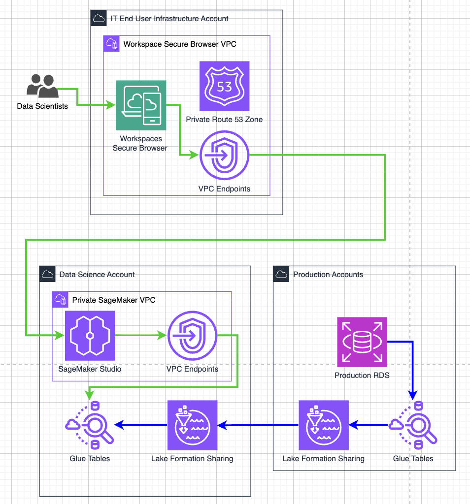
Figure 1: Three-layered security architecture for data exfiltration prevention
iBusiness used Amazon WorkSpaces Secure Browser, a managed, locked-down browser environment. This managed service provides a controlled Chromium-based browser, offering a more cost-effective solution for the company’s use case.
The company configured the Secure Browser to run within a dedicated VPC and subnet in its IT infrastructure account, routing outbound traffic through a network address translation (NAT) gateway. In the secure data science account, iBusiness enforced AWS Identity and Access Management (IAM) policies that restrict access to requests originating only from AWS services or from the NAT gateway’s Elastic IP address. This configuration helps validate that access to the environment is only possible through the Secure Browser. It gives you confidence that data scientists cannot bypass security controls when you implement a similar approach.
Additionally, the Secure Browser was configured to disable file downloads and uploads, disable clipboard access, and disable printing. These controls help prevent data from being transferred to local machines.
Key Secure Browser controls configured:
Building on this foundation, iBusiness restricted activity within the Secure Browser itself to address potential exfiltration through web-based channels.
Although the browser provides a temporary working directory, iBusiness prevented its misuse by implementing strict URL allowlisting. Users can only access *.aws.amazon.com and specific SageMaker AI domains. Other websites, including email and external storage platforms, are blocked, preventing users from uploading data to external services.
Permitted URL patterns:
*.aws.amazon.com.To help verify users cannot move data to other AWS accounts, iBusiness implemented VPC endpoints for AWS Management Console and AWS IAM Identity Center services. These endpoints route traffic privately within the VPC with no internet exposure. They also enforce endpoint policies restricting access to iBusiness’s specific AWS account, giving you control over which accounts data scientists can access.
The company also configured a private Amazon Route 53 hosted zone to redirect console.aws.amazon.com, *.console.aws.amazon.com, and signon.aws.amazon.com to the company’s VPC endpoints instead of public endpoints. To further mitigate DNS-based exfiltration risks, iBusiness configured Amazon Route 53 Resolver DNS Firewall in the SageMaker AI VPC to block DNS queries to non-approved domains, ensuring that only resolution of required AWS service endpoints is permitted.
This configuration helps verify that users can only authenticate into iBusiness’s secured data science account and that access to other AWS accounts is blocked. To further enforce this, iBusiness applied an IAM policy that enhances the IAM policy from Layer 1. This policy helps confirm actions are sourced from an IAM principal originating from a VPC endpoint and denies actions when the target resource belongs to another AWS account, with minimal exceptions for privileged users.
As a final layer of defense, iBusiness secured the SageMaker AI environment itself to prevent data exfiltration through the development environment’s terminal and integrated development environment (IDE) access.
Because SageMaker AI provides terminal and IDE access, it could potentially be used to move data externally. To mitigate this risk, the company removed direct internet access from the SageMaker AI VPC with no NAT gateway or internet routes and configured VPC endpoints for the required AWS services.
This configuration confirms that SageMaker AI can access AWS services internally and function normally while simultaneously blocking direct outbound internet traffic. iBusiness further restricted VPC endpoint policies to allow access only to resources within the organization, providing an additional safeguard against cross-account data movement. VPC endpoint policies allow for granular access to specific AWS resources. For example, allowing users restricted access for s3:PutObject API calls to specific Amazon Simple Storage Service (Amazon S3) buckets depending on the use case.
SageMaker AI network configuration:
By implementing this three-layered security architecture, iBusiness achieved an 80% cost reduction, from $40+ per user monthly for individual VDI environments to $7 per user with Amazon WorkSpaces Secure Browser. The solution also transformed IT operations, reducing provisioning from a 2-day SLA to automatic setup within minutes while eliminating ongoing desktop maintenance overhead.
For data scientists, the approach improved both productivity and security by streamlining data access without compromising protection. This demonstrates how you can strengthen security controls while reducing costs and operational complexity.
Start by assessing your current data access controls, then progressively implement each security layer based on your organization’s specific compliance requirements and risk tolerance.
Post Syndicated from Madhusudan Athinarapu original https://aws.amazon.com/blogs/architecture/dual-token-authentication-for-nakama-game-servers-with-amazon-cognito-on-aws/
When your game server needs both a managed identity provider and its own session system, players face a broken experience if authentication forces a redirect or stalls gameplay. Dual-token authentication for Nakama game servers with Amazon Cognito solves this by connecting two independent session systems, each with its own token lifecycle, without interrupting the player. This post shows you how.
Amazon Cognito handles player identity and Nakama manages game sessions. Cognito issues a JWT, a server-side Go hook validates it and exchanges the verified identity for a Nakama session token. Each token is validated independently on every request. The pattern applies to game servers such as Nakama that support runtime authentication hooks.
The infrastructure wraps Nakama in a default-closed routing layer. Amazon CloudFront serves as the single HTTPS entry point, AWS WAF filters traffic at the edge, an Application Load Balancer (ALB) enforces an explicit route allow-list for HTTP, and a Network Load Balancer (NLB) handles WebSocket TCP passthrough. Nakama runs on Amazon Elastic Container Service (Amazon ECS) on AWS Fargate. In this post, we cover the Cognito configuration, the Go hook, the Terraform infrastructure, and the WebSocket lifecycle controls.
In this post, you learn how to:
The architecture has four layers for authenticating and routing traffic.
The following diagram shows the architecture. Amazon CloudFront is the single entry point, routing HTTP API traffic through an Application Load Balancer (ALB) to Nakama on Amazon ECS, and WebSocket traffic through a Network Load Balancer (NLB) via TCP passthrough.
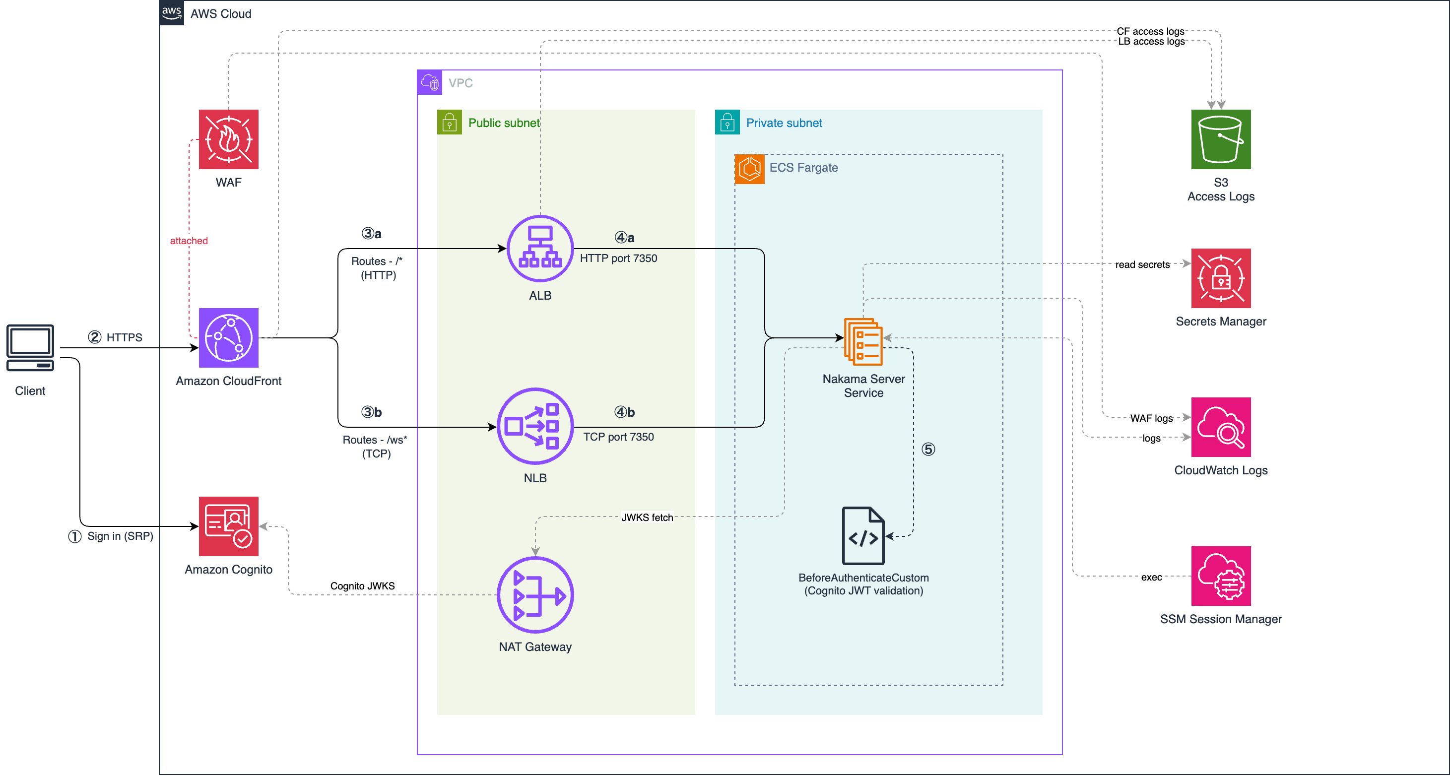
Figure 1. Dual-token authentication architecture for Nakama on AWS.
Traffic flows through the system in six steps:
sub claim as the Nakama user ID. For other API calls: Nakama validates its own session token.The ALB and NLB serve different purposes and cannot be combined into one.
The ALB operates at the HTTP layer (Layer 7). It reads the path, applies listener rules, and returns 403 for unlisted routes.
The NLB operates at the TCP layer (Layer 4) and passes the raw stream to Nakama unchanged. Nakama receives the WebSocket upgrade directly from the client, validates the session token, and manages the connection lifecycle end-to-end.
Amazon CloudFront routes /ws* to the NLB and everything else to the ALB, so each connection type gets the appropriate handling behind a single HTTPS endpoint.
Before you deploy this solution, make sure you have:
The repository includes a browser-based test app (/app) that demonstrates the full sign-up, sign-in, and Nakama token exchange flow.
Amazon Cognito provides a managed user directory that issues JWTs without requiring you to run your own identity server or store credentials. The game server validates the JWT independently on each request, with no callback to Cognito needed. This decouples identity from game sessions: Cognito owns the player’s identity, Nakama owns the game session, and neither system depends on the other at runtime.
Players self-register by calling the Cognito SignUp API from the game client. The User Pool verifies their email before the account becomes active. After sign-in, Cognito returns a JWT access token containing the player’s sub claim (a UUID), which becomes the Nakama user ID in the next step.
Authentication uses the USER_SRP_AUTH flow. The password never leaves the client device. The User Pool App Client is configured as a public client with no client secret, since your game client runs in the browser or a native app where any embedded secret is extractable. With SRP, no secret is needed; security comes from the protocol itself.
After a successful sign-in, Amazon Cognito returns a JWT access token. This token carries the player’s identity claims and is signed with an RSA key pair unique to your User Pool. The sub claim — a UUID generated by Cognito — uniquely identifies the player and becomes the Nakama user ID in the next step.
The auth Terraform module configures the App Client with generate_secret=false and permits only ALLOW_USER_SRP_AUTH and ALLOW_REFRESH_TOKEN_AUTH flows. The resulting JWT access token is short-lived (1 hour by default) and carries the sub, iss, exp, and client_id claims that the Go hook validates in the next step.
Nakama’s server-side runtime supports Go plugins exclusively. The hook in this section is written in Go using Nakama’s runtime.Initializer interface. This is a constraint of the Nakama runtime model.
Once the client has a Cognito JWT, it needs a Nakama session token to make game API calls.
The game server cannot trust the identity claim sent by the client directly. Any client can forge a user ID. JWT validation cryptographically proves the identity was issued by Cognito, preventing player impersonation.
The hook performs five checks in order: token format, algorithm (RS256 only), signature against the JWKS, expiry, and issuer/audience matching your specific User Pool.
Security note: The hook never trusts the identity string sent by the client. It discards it and overwrites the Nakama user ID with the sub claim from the validated JWT. A client that sends a forged sub cannot impersonate another player — the hook ignores the body value entirely.
Amazon Cognito rotates its signing keys periodically. The hook caches keys with a 1-hour TTL. A 30-second re-fetch guard prevents multiple goroutines from calling the JWKS endpoint simultaneously when the cache expires.
The hook registers itself in InitModule, the entry point called by Nakama when the plugin loads:
When the client calls POST /v2/account/authenticate/custom with the Cognito JWT as the id field, Nakama calls beforeAuthenticateCustom before processing the request. If the JWT is valid, the hook sets in.Account.Id = sub and returns. Nakama creates or links the account and returns a session token to the client.
If your server is not Nakama, for example, Colyseus, Photon, or a custom WebSocket server, implement the same five checks (algorithm, signature, expiry, issuer, audience) in your server’s middleware or plugin language. The JWKS endpoint and JWT structure follow the OIDC standard, so any OIDC-compliant identity provider (not only Amazon Cognito) works with this pattern.
The infrastructure is organized into six Terraform modules: network (Amazon Virtual Private Cloud (Amazon VPC), subnets, security groups), compute (Amazon ECS cluster, ALB, NLB, Amazon Elastic Container Registry (Amazon ECR)), auth (Cognito User Pool), cdn (CloudFront distribution), waf-cloudfront (AWS WAF Web ACL), and ops (IAM, AWS Systems Manager access). A bootstrap module creates the S3 state backend and AWS Key Management Service (AWS KMS) key before the main deployment.
Deploy with:
make deploy builds and pushes the Nakama container image to Amazon ECR, then runs terraform apply. The image tag auto-increments from the latest tag in ECR.
The ALB default listener action returns 403. Only the paths in the following table reach Nakama. Requests to unlisted paths are rejected before they reach the game server.
| Priority | Path | Target | Purpose |
| 1 | /healthcheck | Nakama port 7350 | Health monitoring |
| 2 | /v2/account/authenticate/* | Nakama port 7350 | Session bridge: Go hook validates JWT |
| 10 | /v2/* | Nakama port 7350 | Nakama REST API v2 |
| 11 | /v1/* | Nakama port 7350 | Nakama RPC (v1) |
| Default | * | 403 Forbidden | Request never reaches Nakama |
The default-403 posture means a misconfigured client or a scanner probing arbitrary paths gets a 403 at the ALB, not an error from the game server. This limits the attack surface to the explicitly listed API surface.
The network layer enforces two security group rules:
X-CloudFront-Secret header on every request; ALB listener rules reject any request missing the correct value with a 403. The NLB security group applies the same CloudFront managed prefix list restriction at Layer 4.Together, the routing and security group chain means the only path to Nakama is: Internet → CloudFront → AWS WAF → ALB or NLB → ECS. No hop can be skipped.
The NLB TCP passthrough model creates a lifecycle challenge: the NLB drops idle TCP flows after 350 seconds (the AWS default, not configurable). If a player’s connection sits idle, the NLB closes the underlying TCP connection while Nakama still holds an open socket.
The following table describes the four controls that handle this:
| Control | Value | Purpose |
| NLB TCP idle timeout | 350s | NLB drops idle TCP flows. Cannot be changed. |
| Nakama ping interval | 10s | Nakama sends a WebSocket ping every 10s, keeping the TCP flow active. |
| Nakama pong wait | 20s | If the client does not respond to a ping within 20s, Nakama closes the connection. |
| token_expiry_sec | 7200 | Nakama rejects session tokens older than 2 hours at connect time. |
| single_socket | true | A new connection from the same user kills the previous one, preventing stale sessions. |
The 10-second ping interval is the key control. Nakama sends a WebSocket ping frame every 10 seconds on each active connection. The client responds with a pong. This keeps the NLB TCP flow alive well within the 350-second idle timeout. If the client goes silent, Nakama detects the missing pong within 20 seconds and closes the socket cleanly.
The NLB performs TCP passthrough, so there is no opportunity to inspect HTTP headers or validate the session token at the network layer. Nakama validates the session token from the token query parameter when the WebSocket upgrade request arrives. A token older than token_expiry_sec is rejected and the connection is closed before any game messages are processed.
single_socket: true verifies that when a player opens a second connection (after a network drop and reconnect, for example) the server closes the first connection. Without this, a player’s Nakama state can be split across two concurrent connections if the client does not cleanly close the first one.
The four-layer model (keepalive, timeout, session expiry at connect, one-connection-per-user enforcement) applies to any real-time server behind an NLB TCP passthrough: Colyseus, Photon, custom WebSocket backends, or any game server that manages persistent connections. If your server does not have built-in ping/pong, implement application-level heartbeat messages that serve the same role.
Security note: The session token travels as a query parameter (?token=...) in the WebSocket upgrade URL. Query parameters appear in server access logs, load balancer logs, Amazon CloudFront logs, and browser history. Mitigations: all connections use TLS (token encrypted in transit), session tokens are short-lived (2 hours), and single_socket invalidates old connections on reconnect. For production deployments, consider log redaction policies for the token parameter.
To avoid ongoing AWS charges, destroy all resources when you no longer need them.
Destroy the main infrastructure first:
Then destroy the Terraform state backend:
Confirm resources are removed by running terraform state list (should return empty) or checking the AWS Management Console.
In this post, you implemented a dual-token authentication architecture for a Nakama game server on AWS. Amazon Cognito handles player identity through JWT validation; a Go runtime hook bridges verified identity into Nakama sessions; and the infrastructure enforces a routing layer where HTTP API traffic passes through an Application Load Balancer with an explicit allow list and WebSocket connections reach Nakama directly through a Network Load Balancer TCP passthrough.
The four-layer WebSocket lifecycle model can be applied to real-time game servers behind an NLB TCP passthrough, not Nakama exclusively.
For production deployments, consider these next steps:
The full Terraform modules and Go plugin are available in the GitHub repository.
For more on Cognito-based game authentication patterns, refer to Using Amazon Cognito to Authenticate Players for a Game Backend Service and Web application access control patterns using AWS services.
Share your questions and feedback in the comments.
Post Syndicated from Stefan Gromoll original https://aws.amazon.com/blogs/big-data/amazon-redshift-delivers-faster-performance-for-bi-dashboards-and-real-time-analytics/
Business intelligence (BI) dashboards and real-time analytics have become essential tools for making informed decisions quickly. Modern data warehouses must excel at complex, long-running analytical queries and also deliver sub-second response times for the short, ad hoc queries that power interactive and real-time experiences. This matters even more as agents explore and derive new insights from massive amounts of data. From executives monitoring key performance indicators on their morning dashboards to data analysts using agents to explore datasets interactively, the expectation is clear: queries should return results fast and predictably.
Amazon Redshift has long been optimized for these use cases. Over the years, we’ve introduced numerous features designed to improve query performance for BI and real-time analytics workloads, including result caching, materialized views, and automatic workload management (AutoWLM). These capabilities have helped thousands of customers build responsive dashboards and real-time applications on Amazon Redshift. However, we know that when it comes to interactive analytics, every millisecond matters. That’s why we keep focusing on making dashboards load faster and helping exploratory queries return results more quickly.
Today, we’re excited to announce a new performance optimization in Amazon Redshift that improves the response times of low-latency SQL queries, such as those used in real-time analytics applications or generated by BI dashboards. With this enhancement, you can experience improved query latencies because of a reduction in the time Amazon Redshift spends preparing SQL queries for execution. SQL queries start faster, so they return results quicker.
To understand this improvement, let’s first examine one of Amazon Redshift’s existing core performance capabilities: code generation. Code generation is an optimization technique that analyzes each SQL query and generates query-specific C++ code internally. This code is then compiled and executed in parallel across the available Amazon Redshift compute nodes to deliver results back to you. Code generation has been fundamental to Amazon Redshift query performance, executing complex analytical queries with high efficiency.
While code generation results in performant query execution, new queries can experience a one-time compilation overhead the first time they run. Amazon Redshift already caches compiled code, and more than 99% of queries in the Amazon Redshift fleet execute using this cached generated code and experience no compilation overhead. For queries that haven’t been cached yet, the one-time compilation overhead is most noticeable for fast-running queries (for example, millisecond or single-digit second queries), where it can represent a significant portion of total execution time.
With the optimization we announced, Amazon Redshift reduces this compilation overhead. Here’s how it works: when Amazon Redshift receives a query, it first checks if optimized compiled C++ code already exists in the cache from previous executions of similar queries in the Amazon Redshift fleet. If so, it uses that code for best performance. If not, Amazon Redshift now applies a new query compilation optimization that processes new queries immediately using composition. Composition is a technique that generates a lightweight arrangement of pre-existing logic. At the same time, it creates query-specific optimized code that is compiled and executed across available compute resources to boost performance further. Composition removes compilation from the critical path of query execution and provides immediate execution while compilation proceeds in the background. With this optimization, new queries processed by Amazon Redshift start faster and deliver performance consistent with subsequent runs.
This approach ensures that first-time queries start much quicker, while repeated queries continue to benefit from the same leading price-performance that Amazon Redshift code generation delivers.
The best part? No action is necessary for your queries to start benefiting from this performance optimization. This enhancement is now the default for all SQL queries in Amazon Redshift for all users on provisioned clusters or serverless workgroups in all AWS Regions where Amazon Redshift is available at no additional cost.
We analyzed the impact of this new optimization on Amazon Redshift customer clusters. To do so, we measured the compilation time of the 1% of query segments that didn’t get a cache hit in our compilation cache and therefore required compilation. The following chart shows the results. The P50 compilation time before the optimization was 4.3 seconds. With this optimization, the compilation time dropped 25.7x to 170 ms.
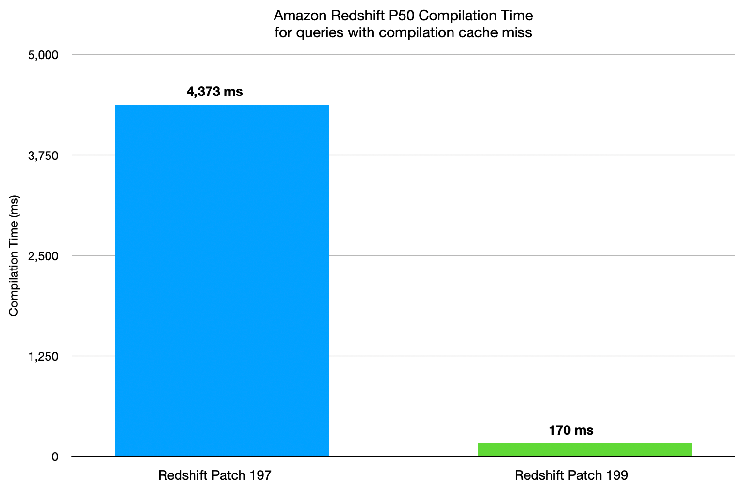
With this optimization, BI dashboards load faster, interactive exploration feels more responsive, and real-time analytics applications can deliver insights with lower latency.
“Following the significant performance improvements that Amazon Redshift demonstrated for cold query execution on our cluster with the FastCompile query performance feature enabled, achieving 2.4x faster query performance with compilation time reduced from 12 seconds to 5 seconds, we have adopted Amazon Redshift as our analytics solution”
— Vijay Hiremath, Group Manager, Business Platforms, Intuit
“As a data platform leader at a leading Chinese liquor company, we rely heavily on Amazon Redshift as our enterprise data warehouse. With diverse analytical query patterns, we faced performance challenges during initial compilation. After testing Redshift’s new cold query compilation enhancement, cold queries now perform nearly as fast as warm queries, with significantly improved speed on diverse queries”
— Yujie Wang, Data Platform Leader, JNC
“In a mid size customer processing about 85 GB of data daily through complex ETL pipelines — multiple tables, mixed DML operations, all landing into our 1.7 TB Amazon Redshift data warehouse, fast compile enhancements accelerated our post-maintenance ETL pipelines by 25%. Now the customer data loads complete faster, data hits analysts sooner for quick decisions”
— Jagan Mohan, Product Engineering Head, Algonomy
To illustrate the impact of this optimization, we simulated a short-running BI-like low-latency workload using a benchmark derived from the industry-standard TPC-DS benchmark. We ran the workload at a relatively small scale of 100 GB on a 3-node RG xlarge Amazon Redshift cluster. At this cluster size and scale, queries finish in milliseconds or single-digit seconds, representing the expected latencies of a typical BI dashboard. The derived TPC-DS benchmark includes 99 different queries that represent a mix of realistic business intelligence workloads, including reporting queries, ad hoc analysis, and data exploration patterns. For this test, we compared a single cold run of these queries on an Amazon Redshift RG cluster with the same run on comparable alternative cloud data warehouses. We launched the warehouses, loaded the data, executed a single run of 99 queries, and measured the total runtime and geometric mean of the queries. No other cluster warm-up or setup was done. This query performance improvement is hardware agnostic. It works on all supported Amazon Redshift hardware instance types, on RA3 and RG on provisioned clusters, and on the hardware that supports serverless workgroups.
The results are shown in table below and summarized in subsequent chart. With this new optimization, Amazon Redshift delivers the fastest runtime and geomean for these short queries at the lowest cost, with up to 8.3x better price-performance than the leading alternative data warehouses for new queries.
| . | Cost / hr | Runtime (sec) | Geomean (sec) | Runtime comparison | Geomean comparison | Geomean price-performance |
| Redshift 3-node RG.xlarge | $2.28 | 235 | 1.7 | baseline | baseline | baseline |
| Alternative Warehouse A | $3.00 | 327 | 2.3 | 1.4x slower | 1.3x slower | 1.7x more expensive |
| Alternative Warehouse B | $4.00 | 538 | 3.4 | 2.3x slower | 2x slower | 3.4x more expensive |
| Alternative Warehouse C | $6.00 | 907 | 5.5 | 3.9x slower | 3.2x slower | 8.3x more expensive |
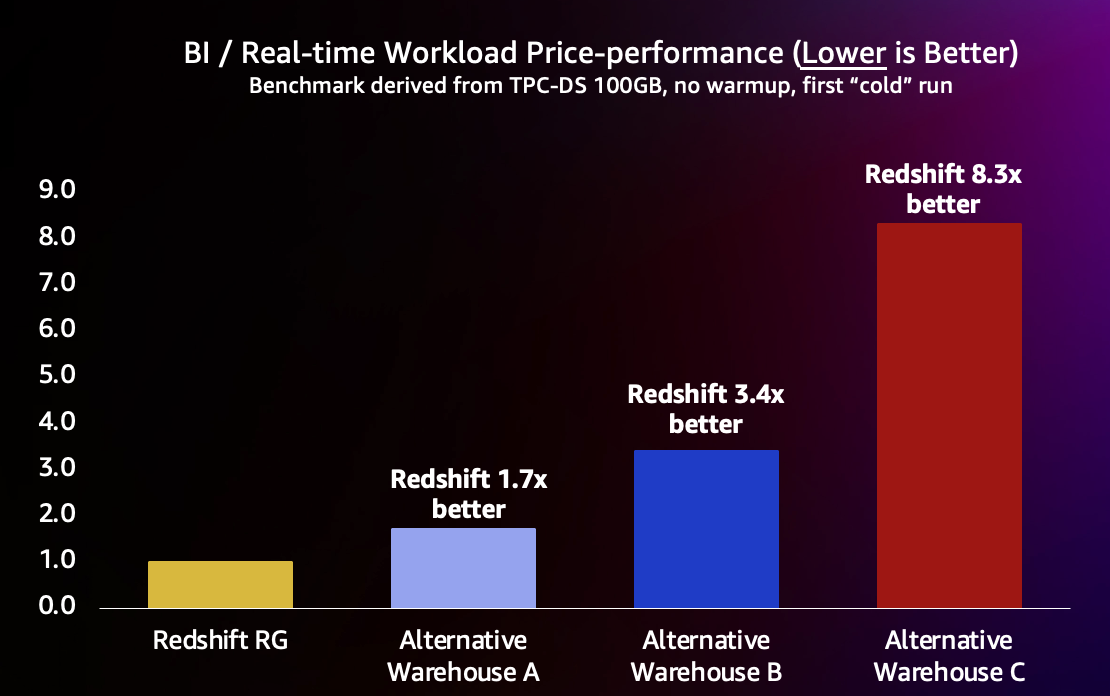
The new query startup optimization in Amazon Redshift continues our commitment to fast performance across analytical workloads. By reducing compilation overhead, we’ve made BI dashboards and real-time analytics applications more responsive, while maintaining the query execution performance that Amazon Redshift is known for.
Because this optimization is automatically enabled for all Amazon Redshift customers, you can start experiencing these benefits immediately. No configuration changes or query rewrites are required. Your existing queries will run faster.
To learn more, visit Amazon Redshift. To get started, you can try Amazon Redshift Serverless and start querying data in minutes without setting up or managing data warehouse infrastructure. For more details on performance best practices, see the Amazon Redshift Database Developer Guide.
The benchmark used in this post is derived from the industry-standard TPC-DS benchmark, and has the following characteristics:
SELECT queries. It does not include maintenance and throughput steps.We call this benchmark the Cloud Data Warehouse Benchmark, and you can reproduce the preceding benchmark results using the scripts, queries, and data available on GitHub. It is derived from the TPC-DS benchmark and is not comparable to published TPC-DS results, because our test results do not comply with the specification.
Each workload has unique characteristics. If you’re starting out, a proof of concept is the best way to understand how Amazon Redshift performs for your requirements. When running your own proof of concept, focus on proper cluster sizing and the right metrics: query throughput (the number of queries per hour) and price performance. You can make a data-driven decision by requesting assistance with a proof of concept or by working with a system integration and consulting partner.
To stay current with the latest developments in Amazon Redshift, subscribe to the What’s New in Amazon Redshift RSS feed.
Post Syndicated from Nidhi Nayak original https://aws.amazon.com/blogs/big-data/optimize-your-tableau-integration-with-amazon-redshift-serverless/
This is a guest blog post co-written by Adiascar Cisneros, from Tableau at Salesforce.
Integrating Tableau with Amazon Redshift Serverless gives you high-performance analytics with serverless scaling and minimal capacity planning. Although automatic scaling handles warehouse management for you, optimization requires a strategic approach to data modeling, security, and query management.
In this post, we provide a guide to help you use Tableau’s Relationships and Amazon Redshift Serverless architecture to deliver sub-second insights while maximizing every Redshift Processing Unit (RPU). We also provide guidance on five key areas: data model architecture for optimal query performance, security configuration and access control, performance optimization through smart configuration, cost management strategies, and query and join optimization techniques.
Before implementing these optimization strategies, make sure you have:
The success of any analytics system begins with its data model. True scalability starts with the end-user experience. Your data model is more than a storage structure. It’s the foundation of dashboard responsiveness. By aligning your database design in Amazon Redshift with your analytical requirements, you empower Tableau to generate highly efficient queries, reducing costs and keeping your users engaged with the data.
When connecting to Amazon Redshift, we recommend using Tableau’s logical data model, specifically Relationships. With Relationship, you can preserve the native level of detail for each table, so Tableau can perform join culling and dynamically query only the specific tables needed for a particular visualization.
When designing your Amazon Redshift schema, implement a well-structured star or snowflake schema, or one big denormalized table where appropriate. This allows Tableau to optimize query execution automatically. Modern Amazon Redshift deployments benefit significantly from Automatic Table Optimization (ATO), which uses AI and machine learning (ML) to continuously monitor and adjust sort keys and distribution keys. To take advantage of ATO, keep sort keys and distribution styles at their default AUTO setting when you create tables. ATO then continuously monitors workload patterns and adjusts keys to improve query performance.
Start by implementing Relationships in your existing workbooks to take advantage of join culling and improved query performance.
Native database drivers provide enhanced security features and better integration with Amazon Redshift capabilities compared to generic ODBC or JDBC alternatives.
The integrity of your analytics relies on the quality of the connection between your platforms. Use the native Amazon Redshift driver rather than generic ODBC or JDBC alternatives. The native driver is specifically engineered to use the advanced capabilities of Amazon Redshift and supports modern security protocols, such as AWS IAM Identity Center, out of the box. By prioritizing the native driver, you verify that your connection uses the latest security patches and performance optimizations, establishing a hardened and efficient entry point for your data. For more information, see Integrate Tableau and Okta with Amazon Redshift using AWS IAM Identity Center.
In Amazon Redshift, cursors are used to retrieve a result set from a query and process the data row-by-row or in smaller chunks rather than loading the entire set into memory at once. For high-scale environments, stable connections depend on how you handle large result sets. In some high-volume scenarios, Amazon Redshift cursors can introduce resource overhead that impacts user concurrency. Monitor your workload and, if necessary, fine-tune your connection configurations using Tableau Data Customization (TDC) files. TDC files are XML configuration files that customize how Tableau connects to your database. Specifically, validate whether disabling cursors improves throughput.
Important: This configuration loads the entire dataset into memory. For large datasets, this might cause performance degradation or out-of-memory errors. Evaluate your dataset size and business requirements before you turn on this setting. This is a key step in tuning your deployment, helping verify that your Amazon Redshift resources remain available and responsive for secure, ad-hoc analysis.
Follow security best practices while deploying Amazon Redshift Serverless. Configure security groups to control inbound access from Tableau Server and Desktop IP ranges. IAM authentication must be the primary method, complemented by SSL/TLS encryption for all connections.
Role-based access control (RBAC) forms the backbone of your security framework:
For authorization, implement a layered security model:
GRANT statements.Audit your current connection types and migrate to the native Amazon Redshift driver if you’re using ODBC or JDBC connections.
Smart configuration spans how much data you query, where you push complex logic, how you design dashboards, and how you tune connections. The following sections cover each area.
To maximize workbook efficiency, start by rigorously managing your data volume. Although Amazon Redshift handles large datasets well, your dashboard should query only what is strictly necessary. Use Tableau Hyper Extracts for production environments to provide a consistent, high-speed cache that offloads repetitive query processing from Amazon Redshift. If a live connection is required, strictly limit your data intake by using Data Source Filters and hiding all unused fields. This helps verify that Tableau generates leaner queries, significantly reducing network latency and processing time.
Next, shift the burden of complexity away from the visualization layer. Materialize calculations within your extracts or push complex logic (especially row-level string manipulations and regex) directly down to the Amazon Redshift database level. By pre-calculating these values before the user ever loads the dashboard, you eliminate expensive runtime processing.
Simplify your logic within Tableau by using native features like CASE statements or Sets rather than complex IF/THEN statements. Testing shows these methods perform significantly faster for grouping dimensions.
Additionally, optimize the rendering process by streamlining your dashboard design:
Optimize Tableau’s performance by enabling connection pooling tailored to your concurrent user count. Configure datetime handling and parallel query execution settings to match your workload patterns.
You can enhance the automatic resource management of Amazon Redshift Serverless through parameter optimization. Key parameters include:
OFF during development to verify you’re testing against live query performance, not cached results. Set it to ON in production.Choosing between extracts and live queries is a foundational architectural decision. We recommend a hybrid approach tailored to specific use cases rather than a one-size-fits-all policy.
Live queries are best for real-time analytics. They use Amazon Redshift Serverless automatic scaling to query massive datasets in place. Use this approach for:
Keep in mind that live connections rely entirely on the database’s performance, so optimizing your Amazon Redshift tables and using materialization techniques within the database is important for maintaining interactivity.
For scenarios when data is static or where query performance is critical, Tableau Hyper Extracts provide a high-speed cache that shifts the processing load from Amazon Redshift to Tableau’s data engine. This is valuable for dashboards with complex calculations (such as row-level string manipulations or heavy aggregations) where an extract can pre-materialize results, effectively baking in the logic before the user ever loads the view. By using extracts for these heavy workloads, you reduce the compute load on Amazon Redshift, lowering costs while delivering sub-second response times to end users.
To maximize efficiency, right-size your extracts for your dashboard’s specific needs:
SELECT * mentality.Balance performance and cost by aligning your connection choice with business freshness requirements and data complexity. Monitor usage patterns to refine this balance over time.
Optimize your star schema joins and queries to reduce execution time and compute costs by using Tableau Relationships. Relationships keep tables separate, allowing Tableau to automatically query only the necessary tables for the fields in the view. Relationships are more flexible and often perform better than joins because they don’t force a row-level merge on all fields.
Inefficient joins and poorly optimized queries force Amazon Redshift to scan unnecessary data, increasing both query execution time and compute costs.
Avoid Custom SQL, which forces Tableau to wrap queries in complex sub-selects. Instead, connect directly to tables or views to let the database optimizer function effectively.
Define primary and foreign keys in your Amazon Redshift schema to allow Tableau to assume referential integrity.
Important: Amazon Redshift does not enforce primary or foreign key constraints. They are informational only, and the query optimizer uses them to generate more efficient execution plans. You’re responsible for data integrity at the application or ETL layer. For more information, see Defining constraints. Assume Referential Integrity is a Tableau setting that tells the engine to trust defined key relationships without validating them at query time, reducing query complexity.
Use Materialized Views to pre-compute heavy aggregations, which reduces execution time for frequently accessed data patterns. For example, create materialized views for common date-based aggregations or customer-level summaries.
Optimize Amazon Redshift Serverless by denormalizing data to minimize complex joins. After you apply these changes, use Tableau’s Performance Recorder to regularly validate your query speeds and identify bottlenecks.
Amazon Redshift Serverless charges in RPU-hours on a per-second basis (60-second minimum), so you only pay for the workloads you run.
Optimizing query volumes and resource usage helps you control Amazon Redshift Serverless costs and maintain predictable spending. To help control compute costs, optimize Tableau queries before they reach Amazon Redshift by using Data Source Filters and ‘Hide All Unused Fields.’ This forces the generation of lean SELECT statements that scan only the necessary rows and columns. Because Amazon Redshift Serverless scales resources based on workload, reducing data volume and complexity at the Tableau source layer can help lower RPU consumption and costs.
For more information, see Amazon Redshift Serverless billing.
Tableau Hyper Extracts act as a cost buffer for high-traffic dashboards. By extracting data into Tableau’s in-memory engine, database costs are typically incurred during scheduled refreshes rather than for every individual user interaction. For live connections, maximize Tableau’s caching architecture by setting server cache policies to “Refresh less often,” ensuring that repetitive dashboard views are served instantly from memory and avoid redundant, billable queries.
Monitor RPU usage patterns and set billing alerts to maintain cost control:
To avoid incurring ongoing charges, delete the resources you created while testing the configurations described in this post.
For more information about managing Amazon Redshift Serverless resources, see Billing for Amazon Redshift Serverless.
This post covered key optimization strategies for Tableau and Amazon Redshift Serverless integration: data model architecture using Relationships, security configuration with native drivers and AWS IAM, performance optimization through extracts and smart configuration, cost management with RPU monitoring, and query optimization techniques.
As AI-driven optimization evolves, staying informed about Amazon Redshift AI features and best practices, including Tableau Pulse, is key. Regularly review your configuration, performance, and security to verify that your Tableau and Amazon Redshift Serverless integration remains secure, cost-effective, and high-performing.
Optimization is an ongoing, iterative process. To keep your environment optimized, regularly review your settings, monitor performance, and adapt as workload patterns evolve. This approach maintains a cost-effective analytics environment that scales with your organization.
Ready to build a secure, high-performance analytics solution that delivers both speed and cost efficiency? Visit the Salesforce and AWS partnership webpage to start scaling your insights today.
Post Syndicated from Micah Walter original https://aws.amazon.com/blogs/aws/aws-weekly-roundup-agentic-cx-designer-for-amazon-connect-customer-ec2-ami-watermarks-open-governance-for-mysql-and-more-june-29-2026/
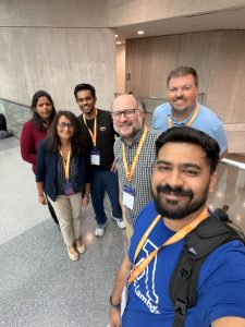 It has been a busy stretch on the AWS Summit circuit. At the New York City Summit, I delivered a workshop called Building AI architectures with AWS Serverless, and it was a lot of fun watching builders wire up agents and serverless services to solve real problems in a single afternoon. This week I am heading down to the Washington, DC Summit, which always puts a spotlight on innovation in the public sector. If you are going to be there, come say hello.
A question I hear a lot at these events is how teams can put AI to work without waiting on a long engineering backlog, and this week’s biggest launch speaks directly to that, with Amazon Connect Customer introducing a no-code way for business teams to design AI powered customer experiences themselves. Now, let’s get into this week’s AWS news.
Headlines
Amazon Connect Customer launched the Agentic CX designer (NLX) in preview, a no-code canvas for designing and deploying AI powered self service experiences. Business teams can build and launch voice and digital experiences that bring agentic and deterministic AI together in one governed flow, going from design to testing and simulation to production ready experiences in weeks rather than months. The launch also includes Live Sync in preview, a patented technology that drives a customer’s web or mobile experience in real time as they speak or type. A caller can complete a form or pull up the right product page without ever leaving the conversation. To see how this reshapes who designs customer experience, read the blog post on how the business user is the new architect of customer experience and visit the Amazon Connect Customer page.
Last week’s launches
Here are some launches and updates from this past week that caught my attention:
For a full list of AWS announcements, be sure to keep an eye on the What’s New with AWS page.
Other AWS news
Here are some additional posts and resources that you might find interesting:
For a full list of AWS blog posts, be sure to keep an eye on the AWS Blogs page.
Looking for ways to connect with builders in person? Check out the AWS Summits coming to a city near you, find a local AWS Community Day led by user groups around the world, and explore tutorials, community content, and ways to grow your skills over at the AWS Builder Center.
That’s all for this week. Check back next Monday for another Weekly Roundup!
-Micah
Post Syndicated from Bruce Schneier original https://www.schneier.com/blog/archives/2026/06/factoring-rsa-keys-with-many-zeros.html
Interesting research on a new class of weak RSA keys: keys with lots of zeros. It turns out that these keys are out in the wild.
The badkeys project is an open-source service that checks public keys for known vulnerabilities. While developing this tool, Hanno collected a massive number of real-world keys from public sources, including Certificate Transparency logs, internet-wide TLS and SSH scans, PGP keys, and many others. By searching this dataset for unexpectedly sparse RSA moduli, we uncovered a large number of keys in the wild with the patterns in Figure 1.
Both patterns include several regularly spaced blocks of all zeros interleaved with seemingly random data. Pattern 1 appears in CT logs for certificates issued to several large organizations, including Yahoo and Verizon, and on some devices running NetApp software. Fortunately, these certificates have already expired, but we still shared our findings with these companies. We wanted to learn more about which product could be responsible for generating these keys, but we did not hear back. Pattern 2 appears on SSH hosts running the CompleteFTP software from EnterpriseDT. The underlying vulnerability affects RSA keys generated using versions 10.0.012.0.0 (Dec 2016Mar 2019) and DSA keys generated with v10.0.023.0.4 (Dec 2016Dec 2023).
These vulnerabilities affect a small minority of hosts on the internet, but the more interesting takeaway is that independent cryptographic implementations failed in similar ways. More implementations may include the same bugs, and so it’s worth tailoring cryptanalytic algorithms for this particular type of failure.
The article doesn’t speculate, but I will. This could be a deliberately designed backdoor, of the sort I wrote about back in 2013. I could imagine some government agency figuring out how to break this class of RSA keys, and then convincing different providers to hand them out to users.
Post Syndicated from LastWeekTonight original https://www.youtube.com/shorts/tsLKSaGj6pY
Post Syndicated from corbet original https://lwn.net/Articles/1078539/
Linus Torvalds released 7.2-rc1
and closed the 7.2 merge window on June 28; by that time, 13,412
non-merge commits had found their way into the mainline. That makes this
the busiest merge window since the 6.7 development cycle in 2024 (15,418
commits, including 2,800 for the entire bcachefs development history).
Just under half of those commits arrived after LWN’s summary of the first half of the merge
window was written. As usual, the commits in the latter part of the
merge window were more heavily focused on fixes, but there were still a lot
of new features and significant changes merged as well.
Post Syndicated from jzb original https://lwn.net/Articles/1079385/
The xsnow
application, which generates an animated snowfall effect (and other
pleasant diversions) for X11 desktops, does not seem like an obvious
channel for political statements. Nevertheless, xsnow’s maintainer
seems to have included a political protest in the program: an
Easter egg that is triggered when the program’s language is set to Russia
(“ru”). One user has complained that this functionality should be
removed from the Debian xsnow
package, but Debian does not seem to have any rules that forbid
such a feature outright.
Post Syndicated from jzb original https://lwn.net/Articles/1080144/
The Kubernetes project has published a blog
post explaining its AI
policy:
The main problem is that AI has made generating code fast but there
has been very little improvement in maintaining code bases. In this
post, we will highlight the ways the Kubernetes community is adapting
to the world of AI assisted coding.The first step of this journey was to develop an AI policy. This
seems mundane and bureaucratic but there were many PRs that derailed
into discussions around AI usage. The AI policy helps steer the
conversation around the project’s stance on AI and provides a clear
signal to contributors on how to use these tools responsibly.
Of note, the project requires disclosure when AI tools have been
used to assist in the creation of a contribution but forbids the use
of listing AI as a co-author or including “assisted-by” or
“co-developed” trailers to attribute work to an LLM tool.
Post Syndicated from jzb original https://lwn.net/Articles/1080143/
Mageia 10 has been
released with the 6.18 Linux kernel, DNF 5.4.0, RPM 4.20.1,
and an increase in hardware requirements for x86 32-bit systems; users now
need a CPU with SSE2 features. See the release
notes for a full list of updates, and the errata page
for known problems.
Post Syndicated from Satish Kamat original https://aws.amazon.com/blogs/compute/building-fault-tolerant-multi-agent-ai-workflows-with-aws-lambda-durable-functions/
Agentic AI workflows coordinate multiple agents that reason, plan, and act across multi-step processes. Each step is expensive, non-deterministic, and unpredictable in latency. Human review gates can pause execution for days. Transient failures are expected, and restarting a half-finished workflow wastes time and money. Duplicate actions, like charging a payment twice or sending the same request again, create financial and compliance risk. Until now, solving these problems meant building custom infrastructure such as state machines, queues, checkpoint stores before writing a single line of business logic.
Prior authorization is one of the most time-consuming steps in healthcare delivery. A provider must get approval from an insurer before certain treatments or medications are covered. The insurer evaluates whether the care is medically necessary, safe, and cost-effective.
Agentic AI is transforming this process. What previously took days — extracting clinical data, evaluating medical necessity, checking payer-specific criteria, and getting physician sign-off — can now be handled by AI agents that pull records, apply guidelines, and draft justification letters automatically.
This post shows how AWS Lambda durable functions can orchestrate an agentic healthcare prior authorization workflow. The pipeline coordinates multiple AI agents, a human review gate, and an external payer submission into a single fault-tolerant function. Using two key patterns — callbacks for human-in-the-loop approvals and asynchronous agent invocations, and polling for long-running external tasks — Lambda durable functions let you focus on the clinical workflow rather than building custom state machines, retry logic, and checkpoint infrastructure.
Lambda durable functions extend the standard Lambda programming model with a checkpoint and replay mechanism. You wrap your handler with the durable execution SDK, which enhances the Lambda context with durable operations such as context.step(), context.waitForCallback(), and context.waitForCondition(). These operations checkpoint progress, handle failures, and suspend execution during wait periods. If a failure occurs or the function resumes after being suspended, Lambda invokes your function again. It restores the previous state by replaying the event handler from the start and skipping over previously completed durable operations. Lambda durable functions offer additional patterns such as parallel execution, durable invocations, and saga-style compensations. Refer to the AWS Durable Execution SDK Developer Guide for the full set of capabilities.
Agentic AI workflows are a natural fit for durable functions because each agent invocation is typically expensive, slow, and prone to transient failures, which are exactly the properties that benefit from automatic checkpointing and replay. Beyond orchestrating agent steps, durable functions can pause the workflow execution for external input. You can suspend the execution until a human approval arrives, or poll an external system for completion with configurable backoff. For on-demand functions, you don’t incur compute charges while execution is suspended (see Lambda pricing for details).
The prior authorization workflow orchestrator coordinates four AI agents, a human review gate, and a payer submission.
waitForCallback(), the function incurs no compute charges while the physician takes minutes, hours, or days to respond.clientRequestToken (shown in the code below) to help prevent duplicate submissions. It then polls the payer’s adjudication status using waitForCondition() with exponential backoff, suspending between each check.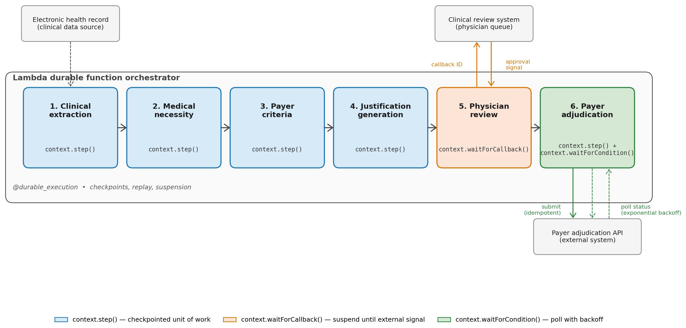
Figure 2. The six-stage prior authorization pipeline, orchestrated by a single Lambda durable function.
The entire pipeline, from agent steps to human review to payer submission and polling, lives in a single function that reads top to bottom:
The orchestrator is designed to handle the failure modes that come up in real workflows:
approved: false, the orchestrator returns a REJECTED status, and no payer submission occurs.waitForCondition() raises a timeout error after the configured attempt limit, which you can catch and route to a manual review queue or compensating action.clientRequestToken derived from the execution ID, retries against the payer are idempotent at the payer API level, which helps prevent duplicate authorization requests.The callback pattern allows the orchestrator to suspend execution and wait for an external signal before resuming. When the durable function reaches a context.waitForCallback(), it sends a unique callbackId to an external system and then suspends. When the external system completes its work, it calls the Lambda API with SendDurableExecutionCallbackSuccess (or SendDurableExecutionCallbackFailure) to resume the orchestrator from where it left off.
In the prior authorization pipeline, this is how the physician review step works. After the justification generation agent produces a letter, the orchestrator emits a callback ID to the clinical review system and suspends. The physician receives the draft in their review queue, reads it, and either approves or rejects it through the review UI. The UI calls the Lambda callback API with the result, and the orchestrator resumes with the approval decision.
Because the function is fully suspended, it incurs no compute charges during the review window, whether that’s 10 minutes or 3 days.
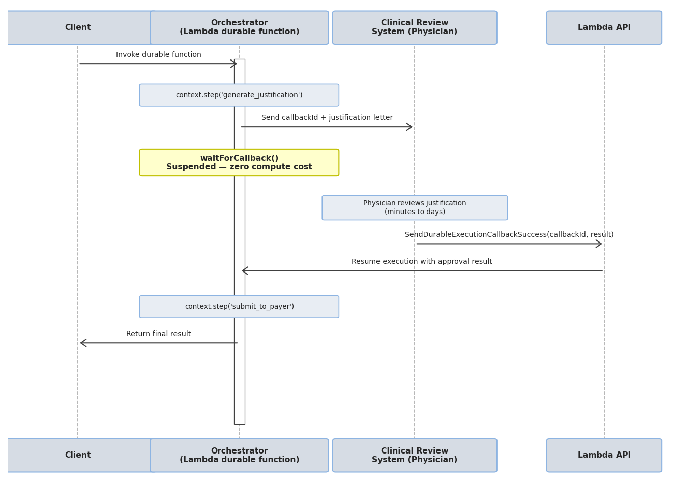
Figure 3. The callback flow for the physician review step. The orchestrator emits a callback ID to the clinical review system and suspends. When the physician approves or rejects, the review system calls SendDurableExecutionCallbackSuccess to resume the orchestrator with the decision.
The callback pattern is appropriate when:
When an external system cannot send a callback, for example a payer API that offers no webhook support, the polling pattern provides an alternative. The orchestrator monitors the long-running task by periodically checking its status using context.waitForCondition().
It runs a check function periodically as configured by a wait strategy and evaluates the result. If the task isn’t complete, suspends for a configurable delay before checking again. The function incurs no compute charges during each wait interval. Each poll result is automatically checkpointed, so on replay the orchestrator skips previously completed checks.
In the prior authorization pipeline, this is how the payer adjudication step works. Most payer APIs accept a submission and return a tracking ID, but don’t push a completion signal back. The orchestrator calls waitForCondition() with the payer’s status API, an exponential backoff strategy (30 seconds to 5 minutes), and a maximum attempt count that covers the payer’s typical adjudication window.
Lambda durable functions provide waitForCondition() with built-in support for configurable backoff strategies, maximum attempt limits, and timeouts, which can help reduce the need for separate polling infrastructure such as scheduled rules, state machines, or custom retry logic.
Figure 4. The polling flow for the payer adjudication step
Polling is appropriate when:
Here are a few implications when using orchestration of agentic workflows with Lambda durable functions:
clientRequestToken, which helps the payer deduplicate on their side. This is an important property when duplicate authorization requests can trigger compliance issues.context.logger) is replay-aware, meaning that it automatically suppresses duplicate log lines during replay.ApproximateRunningDurableExecutions, DurableExecutionDuration, and DurableExecutionFailed, so you can track running workflows, detect failures, and set alarms at the execution level. Lambda also publishes durable execution status change events to Amazon EventBridge (RUNNING, SUCCEEDED, FAILED, TIMED_OUT) for triggering notifications or downstream workflows, and you can enable AWS X-Ray for distributed tracing across the entire execution. For more details, see Monitoring durable functions in the Lambda developer guide.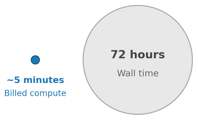
To accelerate building agentic workflow orchestration with Lambda durable functions, you can use the Kiro power for Lambda durable functions or the Agent Plugin for AWS Serverless, which is available in any AI coding assistant tool that supports agent plugins such as Claude Code and Cursor. You can also install agent skills from the plugin individually in any AI coding assistant tool that supports agent skills. This helps your coding agents such as Kiro to:
context.step(), wait_for_callback(), and wait_for_condition() calls based on the described stages.Agentic AI workflows can be non-deterministic, long-running, and failure-prone. Lambda durable functions can help address these challenges by adding checkpointing, replay, and suspension to the Lambda programming model, so completed work is skipped on retry and failures resume exactly where they occurred.
In this post, we walked through a healthcare prior authorization pipeline to illustrate two patterns: Callbacks for human-in-the-loop approvals and asynchronous agent invocations, and polling for monitoring long-running external tasks.
Beyond these two patterns, Lambda durable functions offer additional capabilities for building resilient workflows such as parallel execution, child contexts for isolated execution context for grouping operations, and saga-style compensations. Refer to the Lambda durable functions Developer Guide for the full set of capabilities. For pricing of on-demand and provisioned-concurrency functions, see the Lambda pricing page.
Get started with Lambda durable functions with examples from Serverlessland and install the Agent Plugin for AWS Serverless.
Post Syndicated from jzb original https://lwn.net/Articles/1080075/
Security updates have been issued by AlmaLinux (containernetworking-plugins, golang, kernel, libpng, libpng15, nginx, opencryptoki, perl-IO-Compress, thunderbird, and tigervnc), Debian (chromium, gdcm, incus, libhtml-parser-perl, lxd, openvpn, tor, and xorg-server), Fedora (chromium, docker-buildkit, docker-buildx, dotnet10.0, dotnet8.0, dotnet9.0, krita, ldns, libssh2, liferea, lighttpd, mariadb10.11, mariadb11.8, moby-engine, nginx, nginx-mod-brotli, nginx-mod-fancyindex, nginx-mod-headers-more, nginx-mod-js-challenge, nginx-mod-modsecurity, nginx-mod-naxsi, nginx-mod-vts, openbao, pacemaker, pgadmin4, podman-tui, prometheus-podman-exporter, python-jupyter-server, python-mistune, python-postorius, python-pydantic-settings, python3-docs, python3.14, thunderbird, tigervnc, tinyproxy, and util-linux), Mageia (krb5), Oracle (.NET 10.0, .NET 8.0, .NET 9.0, bind, dracut, fence-agents, firefox, frr, frr10, glib2, glibc, gnutls, golang, kernel, libpng, libpng15, libreoffice, libxml2, libxslt, mod_http2, mysql:8.4, nginx:1.26, openssl, php:8.3, podman, postgresql-jdbc, python3.14, redis, rsync, thunderbird, tomcat, valkey, and vim), Red Hat (osbuild-composer), and SUSE (agama-web-ui, asn1c, assimp, assimp-devel, aws-iam-authenticator, calibre, clamav, corepack24, dovecot22, exiv2, frr, giflib, glances-common, google-osconfig-agent, GraphicsMagick, gvim, haproxy, hydra, ImageMagick, jupyter-nbclassic, kernel, libsoup, libsoup2, libssh2-1, nano, NetworkManager-applet-openvpn, nodejs22, openbabel, opensc, openssl-3, pacemaker, python, python-base, python-doc, python311-pdm, python311-py7zr, python311-pypdf, python36, tar, trivy, util-linux, xen, and xtrabackup).
Post Syndicated from Netflix Technology Blog original https://netflixtechblog.com/genpage-towards-end-to-end-generative-homepage-construction-at-netflix-77146fba8a08
Authors: Lequn Wang, Jiangwei Pan, and Linas Baltrunas
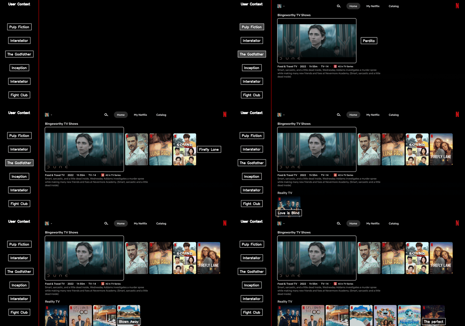
The Netflix homepage is the first thing users see when they open the app and the primary way they discover content to enjoy. Almost every part of it is personalized, including which rows appear, which entities show up within those rows, and how everything is arranged on the page.
Constructing that homepage is a genuinely hard problem. It is not simply producing one ranked list. The homepage is a structured, two-dimensional layout, made up of recommendation rows and the entities within them. Here, an entity can be a movie, show, game, live event, or other recommendable item. Each choice can affect the value of the others. Traditionally, it is built through a complex, multi-stage pipeline, with separate components for candidate generation and ranking at both the row and entity levels.
We saw an opportunity to rethink this design. Large language models have shown that a single generative model can perform diverse tasks just by generating a response to a prompt. Inspired by this prompt-response paradigm, we trained a single generative model to build the homepage by directly answering one question:
Given everything we know about this user and this request, what homepage should we generate to maximize user satisfaction?
We call this approach GenPage. It treats the user history and request context as the prompt, and autoregressively generates the entire homepage as the response (Figure 1). Unlike most generative recommenders, such as TIGER, HSTU, and OneRec, which generate flat ranked lists, GenPage generates the rows, entities, and layout together.
This shift is motivated by several goals:
Bringing GenPage into production at Netflix also required solving challenges specific to industry-scale recommender systems. Because the homepage is generated in real time, serving latency is a primary engineering constraint. We also need to handle entity cold start in a constantly evolving catalog, keep the model fresh as user interests and cultural trends shift, and enforce complex product and business rules on the generated output.
Despite these challenges, GenPage has already had substantial production impact. In an online A/B test against a mature, highly optimized multi-stage production recommender, GenPage delivered statistically significant gains on the core user engagement metric we use for launch decisions, while reducing end-to-end serving latency by 20%.
Offline, two findings stood out. First, enriching the prompt helped more than scaling model capacity in our current regime. Second, RL post-training increased homepage diversity even though diversity was not part of the objective.
We expect this approach to generalize to many personalization settings. In this post, we focus on Netflix homepage construction as a concrete case study, sharing our design, trade-offs, and lessons learned.
Moving from a traditional recommender to a generative transformer requires us to rethink how the data is represented. Similar to how an LLM turns text into tokens, GenPage represents both the user context and the generated homepage as one sequence of discrete tokens (Figure 2). This sequence includes the full structured homepage layout, with multiple rows and the entities inside them, so the model can generate the page holistically rather than scoring each row or entity in isolation.
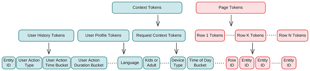
Each training example represents a homepage impression and consists of three components:
Only the context and page are tokenized as model inputs and outputs. Feedback is used to derive supervision signals via our internal reward system (see the Reward system section).
Instead of using an off-the-shelf text tokenizer, we build a domain-specific tokenizer for the homepage construction data. This is a proven approach in recommender systems and other specialized domains including computer vision, biology, and chemistry, where the raw data is not naturally represented as text. Compared with generic text tokenization, this gives us two key advantages:
Context tokens encode user engagement history, user profile, and request context.
We represent user history as a sequence of user actions. For each action, we extract key metadata, including the action type, entity ID, timestamp, and duration. These actions include both explicit signals, such as play, add to My List, and thumbs-up, and implicit signals, such as trailer views or visits to a details page.
User profile tokens capture attributes such as language and profile type. Request context tokens encode signals like time of day, day of week, and device.
Some data sources are too long to include directly as raw token sequences. A user’s full impression history, for example, would be prohibitively expensive to represent in full. In these cases, we use a summarized version. This is a pragmatic trade-off: while GenPage aims to operate on raw inputs as much as possible, handcrafted summaries still introduce a form of prompt engineering into the pipeline. Learning to compress these long data sources end to end is an important direction for future work.
To help the model distinguish between data sources, we insert special tokens that mark the start of each segment. Continuous signals, such as timestamps and durations, are bucketized into discrete ranges to keep the vocabulary finite.
Each entity, such as a show, movie, or game, and each row, such as Korean TV Shows, is represented as a single token. The homepage is serialized in layout order: left to right, then top to bottom. We update the entity and row vocabulary daily to incorporate newly added entities and rows. Entities that are still out of vocabulary at serving time are handled through semantic embedding fusion and fallback tokens, both described later.
In principle, the same paradigm can extend to any output that can be expressed as a linear token sequence. This includes layouts beyond the current two-dimensional structure, such as one-dimensional feeds or mixed layouts, as well as personalized UI components and per-entity outputs such as personalized artwork. We leave these extensions to future work.
To make recommendations responsive to in-session user preferences, the homepage is often generated incrementally, a few rows at a time. Before each pagination request, we append the page tokens from previously generated rows to the prompt, along with the user’s latest engagements on those rows from Netflix’s real-time event-logging infrastructure. This allows the model to generate the next set of recommendations using both the user’s long-term preferences and their most recent in-session behavior.
To quantify the long-term value of a recommendation, we rely on an internal reward system described in prior work. The reward system is tuned through online A/B testing to align with long-term user satisfaction and serves as the primary supervision signal for both supervised and reinforcement learning.
The reward system processes user feedback and assigns a scalar reward for every impressed entity on the homepage. For instance, a TV show binge-watched in one night reflects stronger user satisfaction and receives a higher reward than a movie watched for only 10 minutes. An impressed entity that the user abandons receives a negative reward.
We define the page-level reward as the sum of rewards across all impressed entities on the homepage.
GenPage uses a standard decoder-only transformer architecture, the same general architecture behind many modern LLMs. This choice keeps the model simple and flexible, while also letting us benefit from the broad ecosystem of tooling around transformer training and serving.
One architectural detail is that we untie the input embedding and output projection weights. This is useful because pretraining and post-training place different demands on the logits. Next-token prediction pretraining optimizes a softmax over the vocabulary, while weighted binary classification (WBC) post-training optimizes per-token sigmoid scores, as described below. Untying the weights gives the model more flexibility to adapt to both objectives.
Our training pipeline mirrors the LLM recipe: we first teach the model the “language” of the Netflix homepage through pretraining, then align its outputs with user satisfaction through post-training. For post-training, we explore two alternative approaches: weighted binary classification (WBC) and reinforcement learning (RL).
WBC is simpler to optimize and aligns directly with the entity-level objectives of our production ranking models. RL is harder to evaluate and optimize, but it is the key path to GenPage’s full vision of page-level optimization, with the flexibility to incorporate test-time reasoning and multi-token entity representations.
We pretrain the model with a standard next-token prediction objective: given the context tokens and a prefix of page tokens, the model learns to predict the next page token. This stage focuses on representation learning, teaching the model the relationship between user contexts and successful homepages. Note that our context-page training examples resemble the prompt-response pairs used in LLM supervised fine-tuning (SFT) more than the raw text used in LLM pretraining. We nonetheless call this stage pretraining because we train the model from scratch rather than fine-tuning from an existing checkpoint.
Unlike LLMs, which often face a scarcity of high-quality labeled data, recommender systems have an abundance of user feedback. For pretraining, we use homepage impressions that received positive feedback when served in production, bootstrapping the model to generate pages similar to those produced by the existing production system.
However, pretraining mainly teaches GenPage to imitate the production system. It does not directly optimize the magnitude of the reward, and as GenPage becomes part of production, repeatedly training on pages generated by earlier versions of the model can risk model degeneration. To address these limitations, we explore two post-training approaches.
One effective way to align the generative model with user satisfaction is weighted binary classification (WBC). At a high level, WBC turns generation into token-level value prediction: given the user context and the tokens generated so far, the model learns to estimate the value of generating each possible next row or entity token.
This objective is easier to optimize than page-level RL. By decomposing the homepage into per-token targets, WBC provides token-level credit assignment by construction, rather than requiring RL to infer how each generated decision contributed to the final page-level reward.
This training setup is enabled by our custom tokenization. Each page token corresponds directly to a specific entity or row, making it straightforward to assign a reward. For every impressed entity on the page, our reward system provides a scalar reward based on user feedback. For each impressed row, we derive a row-level reward by aggregating the rewards of the entities in that row.
From each reward, we derive a binary label from its sign, such as positive engagement versus abandonment, and a weight from its magnitude, such as binge-watching receiving a higher weight than a short play. We then optimize a weighted binary cross-entropy loss on the logit for the corresponding token. Under this setup, the logit for a token can be interpreted as the model’s value estimate for generating that token at that position.
Although the model is trained as a value predictor, it can still generate pages autoregressively. At each step, the model scores the candidate next tokens, greedily selects the token with the highest value, and appends it to the prefix. This process repeats token by token until the full homepage is generated.
Our second post-training approach is reinforcement learning (RL). WBC is effective for optimizing entity-level metrics, but it does not directly optimize the homepage as a whole. RL treats page generation as a sequential decision-making problem, allowing the model to optimize a page-level reward while preserving the flexibility of autoregressive generation.
This opens the door to several important capabilities:
Inspired by the RLHF recipe used to align large language models, we adopt a two-step approach. First, we train a reward model that predicts the page-level reward for a generated page. This reward model is distinct from the reward system described earlier. The reward system converts observed user feedback into a scalar reward for a page that was actually shown, whereas the reward model predicts the page-level reward for a generated page without showing it to the user. This prediction is what lets RL optimize against arbitrary candidate pages during training.
Training against a reward model avoids the high variance of off-policy correction on logged or predicted propensities, but introduces the risk of reward hacking. Since the reward model is trained on data generated from the production policy, it is most reliable on pages similar to those the production policy generates. We therefore use a KL penalty to keep the policy close to the pretrained checkpoint, which itself was trained to mimic the production policy. This keeps the pages within the reward model’s region of coverage and limits opportunities for reward hacking.
For the RL algorithm, we adopt Dr. GRPO, a variant of GRPO that mitigates biases in the training objective. To train the model within this framework, we need the following components:
New entities lack the rich interaction data needed to learn robust token embeddings. We address this through two complementary strategies:
At Netflix scale, daily retraining of a large transformer from scratch is prohibitively expensive, but recommendation models must remain fresh to capture shifting trends and new catalog additions. We address this with a multi-cadence incremental training strategy (Figure 3).
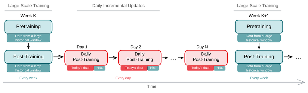
Our training pipeline operates on a cyclic schedule with two distinct rhythms. At a tunable cadence, we conduct a large-scale pretraining and post-training pass on data from a broad historical window. Between these passes, each day we perform an incremental update by continuing post-training from the previous day’s checkpoint, using a mix of the latest day’s data and a sampled subset of past data. This helps the model stay current with new trends and catalog changes while preventing overfitting and catastrophic forgetting.
To manage the daily influx of new tokens (e.g., new entities, rows), we employ fallback tokens. New tokens are initialized using fallback tokens of their type (e.g., [Row_Fallback_Token] for new rows, [Entity_Fallback_Token] for new entities). During training, we randomly replace a small percentage of known tokens with fallback tokens, teaching the model to handle unknown tokens gracefully.
A Netflix homepage must satisfy structural constraints (e.g., organized as a list of rows) as well as product logic such as deduplication, row pinning, and category consistency (e.g., entities in a Comedy row must be comedies). While training signals can encourage rule adherence, they cannot guarantee strict compliance.
We enforce these rules at inference time through constrained decoding. At each autoregressive generation step, we compute a mask of eligible tokens based on the applicable business rules and apply it to the output logits, allowing only rule-compliant tokens to be generated. This is greatly simplified by our custom tokenization: because each entity and row is a single token, business rules map directly to token-level masks, avoiding the multi-token bookkeeping that constrained decoding requires over a text vocabulary. For example, to pin a specific row (e.g., popular games) at a fixed position (e.g., row position 2), we simply mask out all other tokens at that position.
Autoregressive generation ensures that each newly generated token is conditioned on the full preceding context, but generating every entity token one at a time can be expensive. We leverage the structure of the homepage to balance inference efficiency with the amount of contextual information available to each generated token.
Within each row, the first few entities are especially important: they receive the most user attention and strongly shape the row’s perceived quality and theme. To reduce inference latency, we use a hybrid row decoding strategy. The model autoregressively generates only the first few entities in each row. Conditioned on this generated prefix, we obtain logits for all eligible entities in a single forward pass and select the top-scoring remaining entities, subject to the same inference-time business-rule constraints described above.
This approach preserves autoregressive conditioning where it matters most while avoiding the latency and cost of decoding long rows token by token.
We ran a series of ablations on Netflix internal data to understand how different components of GenPage affect model quality. Because the system was developed iteratively, individual ablations span different training configurations and data snapshots, so we report only relative comparisons within each study. Unless otherwise noted, experiments use ~200M-parameter models and report results on a held-out evaluation set.
We compare WBC post-training with and without a preceding next-token-prediction pretraining stage. Figure 4 shows that pretraining yields substantial improvements across all metrics.
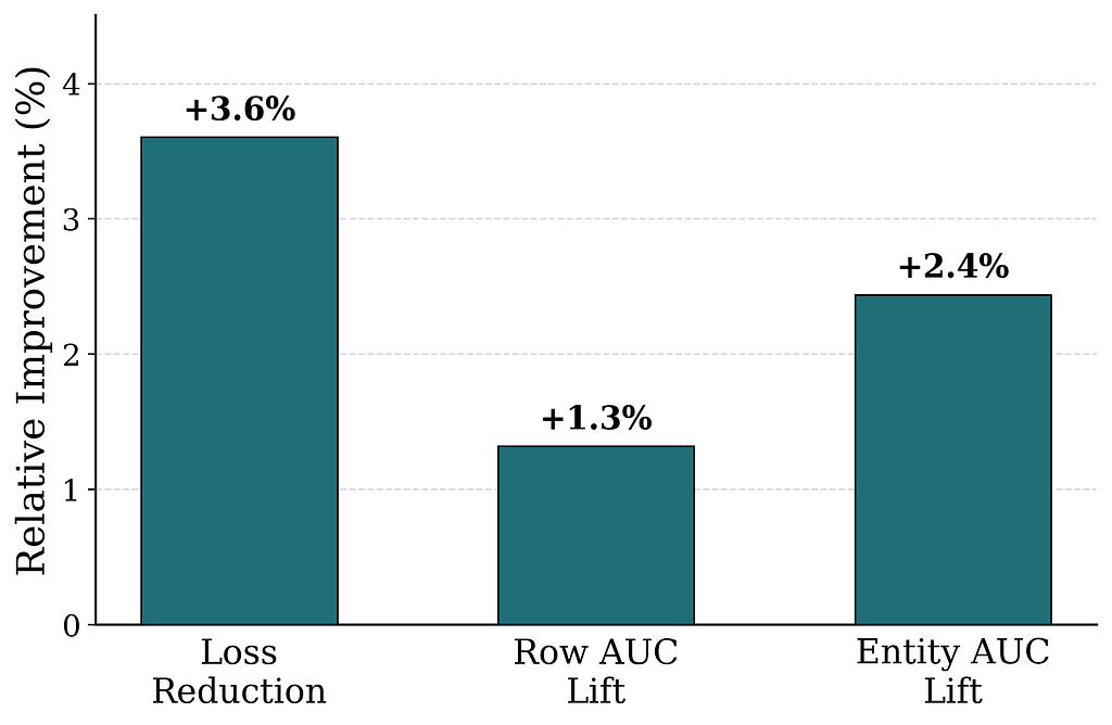
The gains may look small in absolute terms, but they are large in our production regime: setting aside the sample weighting, an Entity AUC lift from 0.91 to 0.92 means that for a randomly drawn pair of impressed entities, the model’s misranking rate drops from 9% to 8% — a magnitude of improvement we rarely observe from a single change on a mature production system. Pretraining the model on the “language” of the Netflix homepage provides a strong initialization for post-training, mirroring the pretrain-then-post-train recipe behind modern LLMs.
We sweep model size from ~120M to ~900M parameters (Figure 5) and report the next-token-prediction loss from pretraining and the WBC loss from post-training. Both losses decrease in a power-law-like fashion, mirroring the scaling trends seen in LLMs. This confirms that the generative approach scales favorably with model size, suggesting that recommendation quality can be further improved by scaling capacity.
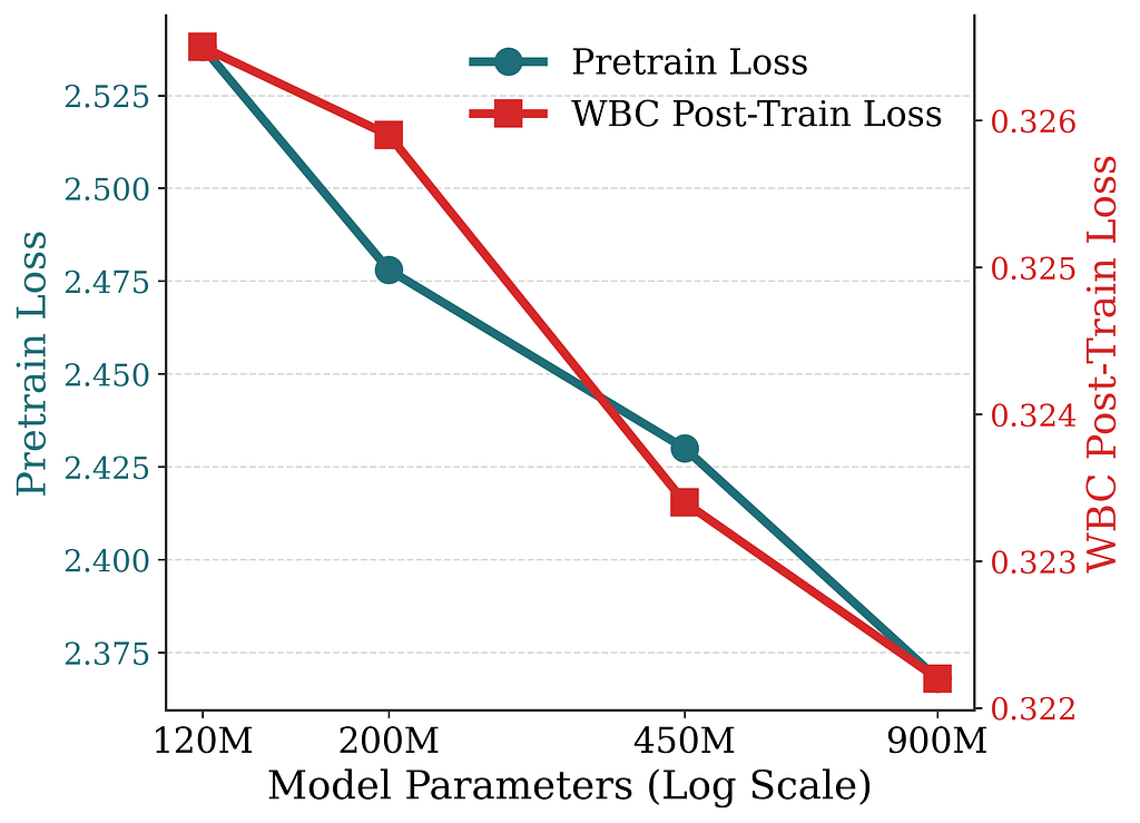
Over the course of development, we progressively enriched the prompt, both by adding new data sources to the context and by refining how each source is tokenized. With model size held fixed, the WBC post-training loss decreases substantially as the context is enriched (Figure 6).
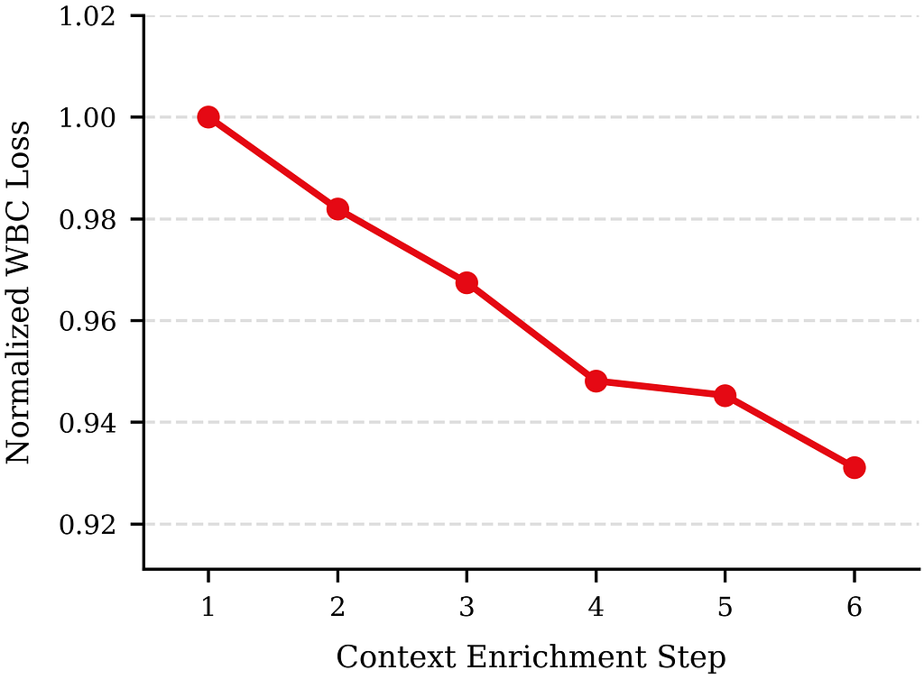
The model-size sweep and the context-enrichment sweep span different axes and are not strictly comparable: the model-size study covers roughly an order of magnitude in parameters, while the context study spans the full trajectory of our prompt design. Even so, the gap between the two is striking. Scaling the model from 120M to 900M parameters reduces WBC loss by roughly 1.3%, whereas the cumulative effect of enriching the context is around 6.9%. In several cases, a single well-designed context addition delivers a larger improvement than the entire ~7.5× model-capacity scaling.
This suggests that, in our regime, enriching the prompt — both what we put in the context and how we tokenize it — yields a substantially larger improvement than scaling model capacity. Personalization quality appears to be bottlenecked first by the information and representation available to the model, and only then by capacity. We expect context enrichment to dominate until the context is saturated, at which point model capacity becomes the primary driver.
In offline evaluations (Figure 7), RL post-training consistently improves the page-level reward over the pretrained checkpoint, but this is largely confirmatory: the reward is computed using the same model the policy is optimizing against. More interestingly, although diversity is not part of the RL objective, homepage diversity — measured via pairwise embedding distance among entities on the page — also increases over the course of training. This suggests that the RL-trained policy is optimizing the page as a whole rather than myopically optimizing each token in isolation.
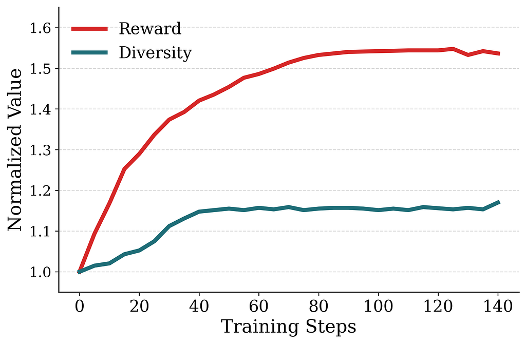
We conducted an online A/B test against the current production homepage recommender using GenPage. In this test, GenPage decoded over the existing production row and entity candidate sets, which help handle many business rules (such as eligibility).
Figure 8 shows the result: all variants delivered statistically significant improvements on the core user engagement metric we use for launch decisions (p < 0.001) against a mature, highly optimized multi-stage production baseline. The variants differed in their training-data configurations; that they all delivered comparable lifts suggests the gain is robust to these design choices rather than dependent on a particular configuration.
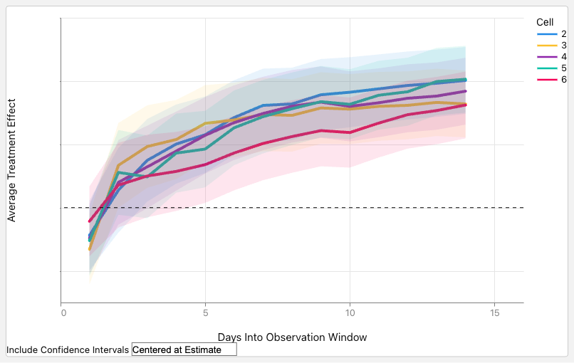
Alongside the engagement wins, we observed unintended shifts in the distribution of impressed entity categories (e.g., new vs. established titles, TV shows vs. movies). These shifts are not necessarily negative, but they are not something we explicitly optimized for, and they warrant deeper investigation. We suspect these shifts reflect GenPage personalizing more precisely than the production stack — consistent with an increase in homepage impression efficiency, i.e., users engaging with what they saw using fewer impressions. This sharper personalization appears to surface production-inherited components (such as the reward system) that aren’t yet aligned with the new generative paradigm. We plan to characterize the drivers of these shifts and, where appropriate, tune these components so the resulting distributions better align with desired product behavior.
We also observed strong responsiveness to in-session signals: the latest in-session actions quickly influenced subsequent recommendations and faded back to long-term preferences after a day or two, confirming that the model effectively attends to action timestamps. This responsiveness emerges naturally from the generative formulation, without the extensive manual feature engineering used in our production stack.
Contrary to the common assumption that generative models are slower, GenPage reduced end-to-end serving latency by 20% relative to the baseline. By replacing multiple ranking stages and heavy feature computation with a single transformer operating on raw tokenized inputs, we eliminated substantial serving complexity and computational overhead. Custom tokenization and hybrid row decoding further reduced the number of decoding steps, and thus latency. The 20% reduction was achieved without exhausting the available optimizations; further reductions are possible, and this headroom can be reinvested in capacity or richer prompts.
We presented GenPage, an early step toward end-to-end generative Netflix homepage construction: representing user context as a tokenized prompt and generating the entire homepage autoregressively in real time. This collapses the traditional multi-stage recommender stack into a single transformer that can be optimized end-to-end.
In online A/B tests against a mature, highly optimized multi-stage production system, GenPage delivered statistically significant gains on the core user engagement metric we use for launch decisions, while reducing end-to-end serving latency by 20%. Achieving this required adapting the LLM training recipe — pretraining followed by WBC or RL post-training — together with a set of domain-specific techniques: custom tokenization for serving efficiency and product control, context injection and semantic embedding fusion for entity cold start, multi-cadence incremental training for model freshness, constrained decoding for business-rule enforcement, and hybrid row decoding for inference efficiency.
Two offline findings stand out. First, in our current regime, enriching the prompt yields a substantially larger improvement than scaling model capacity — a takeaway we expect to generalize to other industry-scale personalization settings, at least until the available context is fully exploited. Second, RL post-training increases homepage diversity even though diversity is not part of the objective — an indication that page-level optimization captures interactions across rows and entities.
Several pieces of the full vision are still in progress: long context still relies on handcrafted summarization, and broader LLM-style capabilities — language, multimodality, and reasoning — have not yet been incorporated. One promising direction here is a hybrid tokenization combining our domain-specific tokens with generic text tokens, retaining structured control while inheriting the strengths of general-purpose LLMs; conceptually, this introduces an additional recommendation modality into an LLM.
More broadly, we expect many advances from the LLM ecosystem to transfer naturally to this setting, and the boundary between an LLM and a recommender system may increasingly blur. Our results suggest this is a viable path toward simpler recommender systems that align more directly with user satisfaction.
Contributors to this work (in alphabetical order): Abhishek Agrawal, Baolin Li, Casey Stella, Daneo Zhang, Dan Zheng, Donnie DeBoer, Fengdi Che, Fernando Amat Gil, Grace Huang, Inbar Naor, Ishita Verma, Jason Uh, Jimmy Patel, Justin Basilico, Lanxi Huang, Lingyi Liu, Liping Peng, Louis Wang, Michelle Kislak, Nathan Kallus, Nicolas Hortiguera, Paran Jain, Qusai Al-Rabadi, Rein Houthooft, Ryan Lee, Santino Ramos, Scarlet Chen, Shaojing Li, Sheallika Singh, Si Cheng, Wei Wang, and ZQ Zhang.

GenPage: Towards End-to-End Generative Homepage Construction at Netflix was originally published in Netflix TechBlog on Medium, where people are continuing the conversation by highlighting and responding to this story.