Tag Archives: Analytics

iostudio delivers key metrics to public sector recruiters with Amazon QuickSight

Post Syndicated from Jon Walker original https://aws.amazon.com/blogs/big-data/iostudio-delivers-key-metrics-to-public-sector-recruiters-with-amazon-quicksight/

This is a guest post by Jon Walker and Ari Orlinsky from iostudio written in collaboration with Sumitha AP from AWS.

iostudio is an award-winning marketing agency based in Nashville, TN. We build solutions that bring brands to life, making content and platforms work together. We serve our customers, who range from small technology startups to government agencies, as a social media strategy partner with in-house video production capabilities, a creative resource that provides data-driven insights about a campaign’s performance, a content marketing machine with connections across the United States, and a sophisticated customer engagement partner.

We wanted to include interactive, real-time visualizations to support recruiters from one of our government clients. Our previous solution offered visualization of key metrics, but point-in-time snapshots produced only in PDF format. We chose Amazon QuickSight because it gave us dynamic and interactive dashboards embedded in our application, while saving us money and development time.

In this post, we discuss how we built a solution using QuickSight that delivers real-time visibility of key metrics to public sector recruiters.

Modernized analytics and reporting

At iostudio, we faced the challenge of modernizing our government client’s static recruitment marketing analytics solution. Given the limitations of the static PDF charts used for its recruitment marketing data, we recognized the opportunity to introduce real-time interactive dashboards to improve insights needed to drive recruitment marketing initiatives. With the solution we built using QuickSight, recruiters are given access to rich visualizations on interactive dashboards in real time, eliminating uncertainty about whether the information they are looking at is accurate.

We created a QuickSight dashboard as a proof of concept, and it surpassed our expectations because of its advanced visualizations. We embedded QuickSight dashboards into our web application, making it seamless for recruiters to log in and get the insights they need. Because we used QuickSight anonymous embedding APIs, we were able to do this without registering and managing all our users in QuickSight. After this initial proof of concept, we gained confidence in our solution quickly, and we were able to build and launch our solution to production within 4–6 weeks. As a result, we reduced our development time by 60%, allowing us to bring this embedded analytics solution to our government client faster. We also saved 75% on our annual external software costs. Switching to QuickSight has enabled us to better serve our customers.

Taking care of sensitive data

iostudio operates in the AWS GovCloud environment because many of our customers are government agencies. This makes protecting customer data even more important. When building our solution for recruiters, we needed to ensure that recruiters can only see data related to the marketing campaigns that are assigned to them. We used row-level security with tag-based rules in QuickSight to restrict data on a per-user basis.

Integrating with AWS

With the AWS technology stack, we were able to create a custom-fit solution using a regionally diverse, service-oriented model to improve our time to deliver interactive reporting to our customers while also trimming costs. With AWS, we aren’t forced to pay for a bundle with services that we don’t use. We can pick what we need, and use what we need with pay-as-you-go pricing.

Our client had previously been using a data integration tool called Pentaho to get data from different sources into one place, which wasn’t an optimal solution. The following diagram illustrates our updated solution architecture using AWS services.

The custom-fit solution that we built uses AWS Lambda to extract data from three key data sources: a referral marketing tool, Google analytics data, and call center operations data. The data lands in an Amazon Simple Storage Service (Amazon S3) bucket, and from there AWS Glue jobs are used to transform the data and load it into another S3 bucket. QuickSight is connected to this data using Amazon Athena, helping us create real-time and interactive dashboards. This end-to-end extract, transform, and load (ETL) process is run with the help of AWS Step Functions, giving us the ability to orchestrate and monitor all the steps of the ETL process seamlessly.

Conclusion

By switching to QuickSight, we were able to provide our client’s recruiters with key metrics in real time, while reducing our development time and cutting costs significantly. Because the components in the architecture are reusable and interoperable, we were able to extend this solution to even more of our customers.

To learn more about how you can embed customized data visuals and interactive dashboards into any application, visit Amazon QuickSight Embedded.


About the Authors

Jon Walker, Senior Director of Engineering, is a native Nashvillian who has been in the technology field for over 19 years. He oversees enterprise-wide system engineering, development, and technology programs for large federal and DoD clients, as well as iostudio’s commercial clients.

Ari Orlinsky, Director of Information Services, leads iostudio’s Information Systems Department, responsible for AWS Cloud, SaaS applications, on-premises technology, risk assessment, compliance, budgeting, and human resource management. With nearly 20 years’ experience in strategic IS and technology operations, Ari has developed a keen enthusiasm for emerging technologies, DOD security and compliance, large format interactive experiences, and customer service communication technologies. As iostudio’s Technical Product Owner across internal and client-facing applications including a cloud-based omni-channel contact center platform, he advocates for secure deployment of applicable technologies to the cloud while ensuring resilient on-premises data center solutions.

Sumitha AP is a Sr. Solutions Architect at AWS. Sumitha works with SMB customers to help them design secure, scalable, reliable, and cost-effective solutions in the AWS Cloud. She has a focus on data and analytics and provides guidance on building analytics solutions on AWS.

Enable business users to analyze large datasets in your data lake with Amazon QuickSight

Post Syndicated from Eliad Maimon original https://aws.amazon.com/blogs/big-data/enable-business-users-to-analyze-large-datasets-in-your-data-lake-with-amazon-quicksight/

This blog post is co-written with Ori Nakar from Imperva.

Imperva Cloud WAF protects hundreds of thousands of websites and blocks billions of security events every day. Events and many other security data types are stored in Imperva’s Threat Research Multi-Region data lake.

Imperva harnesses data to improve their business outcomes. To enable this transformation to a data-driven organization, Imperva brings together data from structured, semi-structured, and unstructured sources into a data lake. As part of their solution, they are using Amazon QuickSight to unlock insights from their data.

Imperva’s data lake is based on Amazon Simple Storage Service (Amazon S3), where data is continually loaded. Imperva’s data lake has a few dozen different datasets, in the scale of petabytes. Each day, TBs of new data is added to the data lake, which is then transformed, aggregated, partitioned, and compressed.

In this post, we explain how Imperva’s solution enables users across the organization to explore, visualize, and analyze data using Amazon Redshift Serverless, Amazon Athena, and QuickSight.

Challenges and needs

A modern data strategy gives you a comprehensive plan to manage, access, analyze, and act on data. AWS provides the most complete set of services for the entire end-to-end data journey for all workloads, all types of data, and all desired business outcomes. In turn, this makes AWS the best place to unlock value from your data and turn it into insight.

Redshift Serverless is a serverless option of Amazon Redshift that allows you to run and scale analytics without having to provision and manage data warehouse clusters. Redshift Serverless automatically provisions and intelligently scales data warehouse capacity to deliver high performance for all your analytics. You just need to load and query your data, and you only pay for the compute used for the duration of the workloads on a per-second basis. Redshift Serverless is ideal when it’s difficult to predict compute needs such as variable workloads, periodic workloads with idle time, and steady-state workloads with spikes.

Athena is an interactive query service that makes it easy to analyze data in Amazon S3 using standard SQL. Athena is serverless, straightforward to use, and makes it simple for anyone with SQL skills to quickly analyze large-scale datasets in multiple Regions.

QuickSight is a cloud-native business intelligence (BI) service that you can use to visually analyze data and share interactive dashboards with all users in the organization. QuickSight is fully managed and serverless, requires no client downloads for dashboard creation, and has a pay-per-session pricing model that allows you to pay for dashboard consumption. Imperva uses QuickSight to enable users with no technical expertise, from different teams such as marketing, product, sales, and others, to extract insight from the data without the help of data or research teams.

QuickSight offers SPICE, an in-memory, cloud-native data store that allows end-users to interactively explore data. SPICE provides consistently fast query performance and automatically scales for high concurrency. With SPICE, you save time and cost because you don’t need to retrieve data from the data source (whether a database or data warehouse) every time you change an analysis or update a visual, and you remove the load of concurrent access or analytical complexity off the underlying data source with the data.

In order for QuickSight to consume data from the data lake, some of the data undergoes additional transformations, filters, joins, and aggregations. Imperva cleans their data by filtering incomplete records, reducing the number of records by aggregations, and applying internal logic to curate millions of security incidents out of hundreds of millions of records.

Imperva had the following requirements for their solution:

  • High performance with low query latency to enable interactive dashboards
  • Continuously update and append data to queryable sources from the data lake
  • Data freshness of up to 1 day
  • Low cost
  • Engineering efficiency

The challenge faced by Imperva and many other companies is how to create a big data extract, transform, and load (ETL) pipeline solution that fits these requirements.

In this post, we review two approaches Imperva implemented to address their challenges and meet their requirements. The solutions can be easily implemented while maintaining engineering efficiency, especially with the introduction of Redshift Serverless.

Imperva’s solutions

Imperva needed to have the data lake’s data available through QuickSight continuously. The following solutions were chosen to connect the data lake to QuickSight:

  • QuickSight caching layer, SPICE – Use Athena to query the data into a QuickSight SPICE dataset
  • Redshift Serverless – Copy the data to Redshift Serverless and use it as a data source

Our recommendation is to use a solution based on the use case. Each solution has its own advantages and challenges, which we discuss as part of this post.

The high-level flow is the following:

  • Data is continuously updated from the data lake into either Redshift Serverless or the QuickSight caching layer, SPICE
  • An internal user can create an analysis and publish it as a dashboard for other internal or external users

The following architecture diagram shows the high-level flow.

High-level flow

In the following sections, we discuss the details about the flow and the different solutions, including a comparison between them, which can help you choose the right solution for you.

Solution 1: Query with Athena and import to SPICE

QuickSight provides inherent capabilities to upload data using Athena into SPICE, which is a straightforward approach that meets Imperva’s requirements regarding simple data management. For example, it suits stable data flows without frequent exceptions, which may result in SPICE full refresh.

You can use Athena to load data into a QuickSight SPICE dataset, and then use the SPICE incremental upload option to load new data to the dataset. A QuickSight dataset will be connected to a table or a view accessible by Athena. A time column (like day or hour) is used for incremental updates. The following table summarizes the options and details.

Option Description Pros/Cons
Existing table Use the built-in option by QuickSight. Not flexible—the table is imported as is in the data lake.
Dedicated view

A view will let you better control the data in your dataset. It allows joining data, aggregation, or choosing a filter like the date you want to start importing data from.

Note that QuickSight allows building a dataset based on custom SQL, but this option doesn’t allow incremental updates.

Large Athena resource consumption on a full refresh.
Dedicated ETL

Create a dedicated ETL process, which is similar to a view, but unlike the view, it allows reuse of the results in case of a full refresh.

In case your ETL or view contains grouping or other complex operations, you know that these operations will be done only by the ETL process, according to the schedule you define.

Most flexible, but requires ETL development and implementation and additional Amazon S3 storage.

The following architecture diagram details the options for loading data by Athena into SPICE.

Architecture diagram details the options for loading data by Athena into SPICE

The following code provides a SQL example for a view creation. We assume the existence of two tables, customers and events, with one join column called customer_id. The view is used to do the following:

  • Aggregate the data from daily to weekly, and reduce the number of rows
  • Control the start date of the dataset (in this case, 30 weeks back)
  • Join the data to add more columns (customer_type) and filter it
CREATE VIEW my_dataset AS
SELECT DATE_ADD('day', -DAY_OF_WEEK(day) + 1, day) AS first_day_of_week,
       customer_type, event_type, COUNT(events) AS total_events
FROM my_events INNER JOIN my_customers USING (customer_id)
WHERE customer_type NOT IN ('Reseller')
      AND day BETWEEN DATE_ADD('DAY',-7 * 30 -DAY_OF_WEEK(CURRENT_DATE) + 1, CURRENT_DATE)
      AND DATE_ADD('DAY', -DAY_OF_WEEK(CURRENT_DATE), CURRENT_DATE)
GROUP BY 1, 2, 3

Solution 2: Load data into Redshift Serverless

Redshift Serverless provides full visibility to the data, which can be viewed or edited at any time. For example, if there is a delay in adding data to the data lake or the data isn’t properly added, with Redshift Serverless, you can edit data using SQL statements or retry data loading. Redshift Serverless is a scalable solution that doesn’t have a dataset size limitation.

Redshift Serverless is used as a serving layer for the datasets that are to be used in QuickSight. The pricing model for Redshift Serverless is based on storage utilization and the run of queries; idle compute resources have no associated cost. Setting up a cluster is simple and doesn’t require you to choose node types or amount of storage. You simply load the data to tables you create and start working.

To create a new dataset, you need to create an Amazon Redshift table and run the following process every time data is added:

  1. Transform the data using an ETL process (optional):
    • Read data from the tables.
    • Transform to the QuickSight dataset schema.
    • Write the data to an S3 bucket and load it to Amazon Redshift.
  2. Delete old data if it exists to avoid duplicate data.
  3. Load the data using the COPY command.

The following architecture diagram details the options to load data into Redshift Serverless with or without an ETL process.

Architecture diagram details the options to load data into Redshift Serverless with or without an ETL process

The Amazon Redshift COPY command is simple and fast. For example, to copy daily partition Parquet data, use the following code:

COPY my_table
FROM 's3://my_bucket/my_table/day=2022-01-01'
IAM_ROLE 'my_role' 
FORMAT AS PARQUET

Use the following COPY command to load the output file of the ETL process. Values will be truncated according to Amazon Redshift column size. The column truncation is important because, unlike in the data lake, in Amazon Redshift, the column size must be set. This option prevents COPY failures:

COPY my_table
FROM 's3://my_bucket/my_table/day=2022-01-01'
IAM_ROLE 'my_role' 
FORMAT AS JSON GZIP TRUNCATECOLUMNS

The Amazon Redshift COPY operation provides many benefits and options. It supports multiple formats as well as column mapping, escaping, and more. It also allows more control over data format, object size, and options to tune the COPY operation for improved performance. Unlike data in the data lake, Amazon Redshift has column length specifications. We use TRUNCATECOLUMNS to truncates the data in columns to the appropriate number of characters so that it fits the column specification.

Using this method provides full control over the data. In case of a problem, we can repair parts of the table by deleting old data and loading the data again. It’s also possible to use the QuickSight dataset JOIN option, which is not available in SPICE when using incremental update.

Additional benefit of this approach is that the data is available for other clients and services looking to use the same data, such as SQL clients or notebooks servers such as Apache Zeppelin.

Conclusion

QuickSight allows Imperva to expose business data to various departments within an organization. In the post, we explored approaches for importing data from a data lake to QuickSight, whether continuously or incrementally.

However, it’s important to note that there is no one-size-fits-all solution; the optimal approach will depend on the specific use case. Both options—continuous and incremental updates—are scalable and flexible, with no significant cost differences observed for our dataset and access patterns.

Imperva found incremental refresh to be very useful and uses it for simple data management. For more complex datasets, Imperva has benefitted from the greater scalability and flexibility provided by Redshift Serverless.

In cases where a higher degree of control over the datasets was required, Imperva chose Redshift Serverless so that data issues could be addressed promptly by deleting, updating, or inserting new records as necessary.

With the integration of dashboards, individuals can now access data that was previously inaccessible to them. Moreover, QuickSight has played a crucial role in streamlining our data distribution processes, enabling data accessibility across all departments within the organization.

To learn more, visit Amazon QuickSight.


About the Authors

Eliad Maimon is a Senior Startups Solutions Architect at AWS in Tel-Aviv with over 20 years of experience in architecting, building, and maintaining software products. He creates architectural best practices and collaborates with customers to leverage cloud and innovation, transforming businesses and disrupting markets. Eliad is specializing in machine learning on AWS, with a focus in areas such as generative AI, MLOps, and Amazon SageMaker.

Ori Nakar is a principal cyber-security researcher, a data engineer, and a data scientist at Imperva Threat Research group. Ori has many years of experience as a software engineer and engineering manager, focused on cloud technologies and big data infrastructure.

Enforce boundaries on AWS Glue interactive sessions

Post Syndicated from Nicolas Jacob Baer original https://aws.amazon.com/blogs/big-data/enforce-boundaries-on-aws-glue-interactive-sessions/

AWS Glue interactive sessions allow engineers to build, test, and run data preparation and analytics workloads in an interactive notebook. Interactive sessions provide isolated development environments, take care of the underlying compute cluster, and allow for configuration to stop idling resources.

Glue interactive sessions provides default recommended configurations, and also allows users to customize the session to meet their needs. For example, you can provision more workers to experiment on a larger dataset or set the idle timeout for long-running workloads. With the flexibility to change these options depending on the workload, you may need ensure that the options are changed within specific boundaries and apply a control mechanism.

In this post, we present the process of deploying a reusable solution to enforce AWS Glue interactive session limits on three options: connection, number of workers, and maximum idle time. The first option addresses the need for applying custom inspection and controls on traffic, for example by enforcing an interactive session to only be run inside a VPC. The other two enforce limits on costs and usage of AWS Glue resources by enforcing an upper boundary on the number of workers and idle time per session. You can further extend the solution for other properties or services within AWS Glue.

Overview of solution

The proposed architecture is built on serverless components and runs whenever a new AWS Glue interactive session is created.

Architecture Diagram of the Solution

The workflow steps are as follows:

  1. A data engineer creates a new AWS Glue interactive session either through the AWS Management Console or in a Jupyter notebook locally.
  2. The interactive session produces a new event to AWS CloudTrail for the CreateSession event with all relevant information to identify and inspect a session as soon as the session is initiated.
  3. An Amazon EventBridge rule filters the CloudTrail events and invokes an AWS Lambda function to inspect the CreateSession event.
  4. The Lambda function inspects the CreateSession event and checks for all defined boundary conditions. Currently, the boundaries configurable with this solution are limited to maximum number of workers, idle timeout in minutes, and deployment with connection enforced.
  5. If any of the defined boundary conditions are not met, for example too many workers are provisioned for the session, depending on the provided configuration, the function ends the interactive session immediately and sends an email via Amazon Simple Notification Service (Amazon SNS). If the session hasn’t started yet, the function will wait for it to start before taking any action.
  6. If the session was stopped, an email is sent to an SNS topic. There is no information available in the interactive session notebook on the reason for the ending of the session. Therefore, additional context information is provided through the SNS topic to the data engineers.
  7. If the function fails, the sessions are logged in a dead-letter queue inside Amazon Simple Queue Service (Amazon SQS). Furthermore, the queue is monitored and in case of a message, it will trigger an Amazon CloudWatch alarm.

The following steps walk you through how to build and deploy the solution. The code is available in the GitHub repo.

Prerequisites

For this walkthrough, you should have the following prerequisites:

Overview of the deployed resources

All the necessary resources are defined in an AWS CloudFormation file located under cfn/template.yaml. To deploy those resources, we use AWS Serverless Application Model (AWS SAM), which enables us to conveniently build and package all the dependencies and also manages the AWS CloudFormation steps for us.

The CloudFormation stack deploys the following resources:

  • A Lambda function with its library, both defined under the directory src/functions. The function is the control. It will validate that the session is started within the limits defined.
  • An EventBridge rule. This event listens to CloudTrail and in case of a new interactive session, will trigger the control Lambda function.
  • An SQS dead-letter queue (DLQ) attached to the Lambda function. This keeps a record of events that triggered a Lambda function failure.
  • Two CloudWatch alarms monitoring the Lambda function failures and the messages in the DLQ.

If notification via email is enabled, two more resources are deployed:

Additionally, AWS CloudFormation deploys all the necessary AWS Identity and Access Management (IAM) roles and policies, and an AWS Key Management Service (AWS KMS) key to ensure that the exchanged data is encrypted.

Deploy the solution

To facilitate the deployment lifecycle, including the setup of the user local environment, we provide a Makefile that describes all the necessary steps. Make sure you have your AWS credentials renewed and have access to your account. For more information, refer to Configuration and credential file settings.

  • Explore the Makefile and adjust the Region and stack name as needed by modifying the values of the variables AWS_REGION and STACK_NAME.
  • Set KILL_SESSION = "True" if you want to immediately stop the interactive session that has been found out of boundaries. Allowed values are True or False; the default is True.
  • Set NOTIFICATION_EMAIL_ADDRESS = <[email protected]> in the Makefile if you want get notified when a session has been found out of boundaries.
  • Set values for your controls:
    • ENFORCE_VPC_CONNECTION to stop sessions not running inside a VPC (true or false).
    • MAX_WORKERS to set the maximum number of workers for a session (numeric).
    • MAX_IDLE_TIMEOUT_MINUTES to define the maximum idle time for sessions in minutes (numeric).
  • Install all the prerequisite libraries:
    make install-pre-requisites

    These will be installed under a newly created Python virtual environment inside this repository in the directory .venv.

  • Deploy the new stack:
    make deploy

    This command will complete the following tasks:

    • Check if the prerequisites are met.
    • Perform pytest unittest on the Python files.
    • Validate the CloudFormation template.
    • Build the artifacts (Lambda function and Lambda layers).
    • Deploy the resources via AWS SAM.

Test the solution

Refer to Introducing AWS Glue interactive sessions for Jupyter for information about running an interactive session. If you follow the instructions in the post (see the section Run your first code cell and author your AWS Glue notebook), the initialization of the interactive session should fail with an error similar to the following.

Example of code in the cell:

from awsglue.context import GlueContext
from awsglue.job import Job
from awsglue.transforms import *
from awsglue.utils import getResolvedOptions
from pyspark.context import SparkContext
sc3 = SparkContext.getOrCreate()
glueContext1 = GlueContext(sc3)
spark = glueContext1.spark_session
job = Job(glueContext1)

Received output:

Authenticating with profile=XXXXXXXX
glue_role_arn defined by user: arn:aws:iam::XXXXXXXXXX:role/XXXXXXXX
Trying to create a Glue session for the kernel.
Worker Type: G.1X
Number of Workers: 5
Session ID: XXXXXXXXXXXXX
Applying the following default arguments:
--glue_kernel_version 0.35
--enable-glue-datacatalog true
Waiting for session xxxxxxxxx to get into ready status...
Session xxxxxxxxx has been created
Exception encountered while running statement: An error occurred (EntityNotFoundException) when calling the GetStatement operation: Session ID xxxxxxxxx not found

If you enabled the email feature, you should also get an email notification.

You can also check on the AWS Glue console that your session ID isn’t listed.

Clean up

Clean up the deployed resources by running the following command:

make clean-up

Note that the resources deployed from following the recommended post, Introducing AWS Glue interactive sessions for Jupyter, will not be removed with the previous command.

Limitations

The delivery guarantee for CloudTrail events to EventBridge are best effort. This means CloudTrail will attempt to deliver all events to EventBridge, but in some rare cases, an event might not be delivered. For more information, refer to Events from AWS services.

Conclusion

This post described how to build, deploy, and test a solution to enforce boundary conditions on AWS Glue interactive sessions in order to enforce constraints on the number of workers, idle timeouts, and AWS Glue connection.

You can adapt this solution based on your needs and further extend it to allow controls on other options.

To learn more about how to use AWS Glue interactive sessions, refer to Introducing AWS Glue interactive sessions for Jupyter and Author AWS Glue jobs with PyCharm using AWS Glue interactive sessions.


About the Authors

Nicolas Jacob Baer is a Senior Cloud Application Architect with a strong focus on data engineering and machine learning, based in Switzerland. He works closely with enterprise customers to design data platforms and build advanced analytics/ml use-cases.

Luca Mazzaferro is a Senior DevOps Architect at Amazon Web Services. He likes to have infrastructure automated, reproducible and secured. In his free time he likes to cook, especially pizza.

Kemeng Zhang is a Cloud Application Architect with a strong focus on machine learning and UX, based in Switzerland. She works closely with customers to design user experiences and build advanced analytics/ml use-cases.

Mark Walser, a Senior Global Data Architect at Amazon Web Services, collaborates with customers to develop innovative Big Data solutions that solve business problems and speed up the adoption of AWS services. Outside of work, he finds pleasure in running, swimming, and all things related to technology.

Gal blog picGal Heyne is a Product Manager for AWS Glue with a strong focus on AI/ML, data engineering and BI, based in California. She is passionate about developing a deep understanding of customer’s business needs and collaborating with engineers to design easy to use data products.

Get started managing partitions for Amazon S3 tables backed by the AWS Glue Data Catalog

Post Syndicated from Anderson dos Santos original https://aws.amazon.com/blogs/big-data/get-started-managing-partitions-for-amazon-s3-tables-backed-by-the-aws-glue-data-catalog/

Large organizations processing huge volumes of data usually store it in Amazon Simple Storage Service (Amazon S3) and query the data to make data-driven business decisions using distributed analytics engines such as Amazon Athena. If you simply run queries without considering the optimal data layout on Amazon S3, it results in a high volume of data scanned, long-running queries, and increased cost.

Partitioning is a common technique to lay out your data optimally for distributed analytics engines. By partitioning your data, you can restrict the amount of data scanned by downstream analytics engines, thereby improving performance and reducing the cost for queries.

In this post, we cover the following topics related to Amazon S3 data partitioning:

  • Understanding table metadata in the AWS Glue Data Catalog and S3 partitions for better performance
  • How to create a table and load partitions in the Data Catalog using Athena
  • How partitions are stored in the table
  • Different ways to add partitions in a table on the Data Catalog
  • Partitioning data stored in Amazon S3 while ingestion and catalog

Understanding table metadata in the Data Catalog and S3 partitions for better performance

A table in the AWS Glue Data Catalog is the metadata definition that organizes the data location, data type, and column schema, which represents the data in a data store. Partitions are data organized hierarchically, defining the location where the data for a particular partition resides. Partitioning your data allows you to limit the amount of data scanned by S3 SELECT, thereby improving performance and reducing cost.

There are a few factors to consider when deciding the columns on which to partition. For example, if you’re using columns as filters, don’t use a column that is partitioning too finely, or don’t choose a column where your data is heavily skewed to one partition value. You can partition your data by any column. Partition columns are usually designed by a common query pattern in your use case. For example, a common practice is to partition the data based on year/month/day because many queries tend to run time series analyses in typical use cases. This often leads to a multi-level partitioning scheme. Data is organized in a hierarchical directory structure based on the distinct values of one or more columns.

Let’s look at an example of how partitioning works.

Files corresponding to a single day’s worth of data are placed under a prefix such as s3://my_bucket/logs/year=2023/month=06/day=01/.

If your data is partitioned per day, every day you have a single file, such as the following:

  • s3://my_bucket/logs/year=2023/month=06/day=01/file1_example.json
  • s3://my_bucket/logs/year=2023/month=06/day=02/file2_example.json
  • s3://my_bucket/logs/year=2023/month=06/day=03/file3_example.json

We can use a WHERE clause to query the data as follows:

SELECT * FROM table WHERE year=2023 AND month=06 AND day=01

The preceding query reads only the data inside the partition folder year=2023/month=06/day=01 instead of scanning through the files under all partitions. Therefore, it only scans the file file1_example.json.

Systems such as Athena, Amazon Redshift Spectrum, and now AWS Glue can use these partitions to filter data by value, eliminating unnecessary (partition) requests to Amazon S3. This capability can improve the performance of applications that specifically need to read a limited number of partitions. For more information about partitioning with Athena and Redshift Spectrum, refer to Partitioning data in Athena and Creating external tables for Redshift Spectrum, respectively.

How to create a table and load partitions in the Data Catalog using Athena

Let’s begin by understanding how to create a table and load partitions using DDL (Data Definition Language) queries in Athena. Note that to demonstrate the various methods of loading partitions into the table, we need to delete and recreate the table multiple times throughout the following steps.

First, we create a database for this demo.

  1. On the Athena console, choose Query editor.

If this is your first time using the Athena query editor, you need to configure and specify an S3 bucket to store the query results.

  1. Create a database with the following command:
CREATE DATABASE partitions_blog;

  1. In the Data pane, for Database, choose the database partitions_blog.
  2. Create the table impressions following the example in Hive JSON SerDe. Replace <myregion> in s3://<myregion>.elasticmapreduce/samples/hive-ads/tables/impressions with the Region identifier where you run Athena (for example, s3://us-east-1.elasticmapreduce/samples/hive-ads/tables/impressions).
  3. Run the following query to create the table:
CREATE EXTERNAL TABLE impressions (
    requestbegintime string,
    adid string,
    impressionid string,
    referrer string,
    useragent string,
    usercookie string,
    ip string,
    number string,
    processid string,
    browsercookie string,
    requestendtime string,
    timers struct
                <
                 modellookup:string, 
                 requesttime:string
                >,
    threadid string, 
    hostname string,
    sessionid string
)   
PARTITIONED BY (dt string)
ROW FORMAT SERDE 'org.apache.hive.hcatalog.data.JsonSerDe'
LOCATION 's3://us-east-1.elasticmapreduce/samples/hive-ads/tables/impressions';

The following screenshot shows the query in the query editor.

  1. Run the following query to review the data:
SELECT * FROM impressions;

You can’t see any results because the partitions aren’t loaded yet.

If the partition isn’t loaded into a partitioned table, when the application downloads the partition metadata, the application will not be aware of the S3 path that needs to be queried. For more information, refer to Why do I get zero records when I query my Amazon Athena table.

  1. Load the partitions using the command MSCK REPAIR TABLE.

The MSCK REPAIR TABLE command was designed to manually add partitions that are added to or removed from the file system, such as HDFS or Amazon S3, but are not present in the metastore.

  1. Query the table again to see the results.

After the MSCK REPAIR TABLE command scans Amazon S3 and adds partitions to AWS Glue for Hive-compatible partitions, the records under the registered partitions are now returned.

How partitions are stored in the table metadata

We can list the table partitions in Athena by running the SHOW PARTITIONS command, as shown in the following screenshot.

We also can see the partition metadata on the AWS Glue console. Complete the following steps:

  1. On the AWS Glue console, choose Tables in the navigation pane under Data Catalog.
  2. Choose the impressions table in the partitions_blog database.
  3. On the Partitions tab, choose View Properties next to a partition to view its details.

The following screenshot shows an example of the partition properties.

We can also get the partitions using the AWS Command Line Interface (AWS CLI) command get-partitions, as shown in the following screenshot.

From the get-partitions, the element “Values” defines the partition value and “Location” defines the S3 path to be queried by the application:

"Values": [
                "2009-04-12-19-05"
            ]

When querying the data from the partition dt="2009-04-12-19-05", the application lists and reads only the files in the S3 path s3://us-east-1.elasticmapreduce/samples/hive-ads/tables/impressions/dt="2009-04-12-19-05".

Different ways to add partitions in a table on the Data Catalog

There are multiple ways to load partitions into the table. You can create tables and partitions directly using the AWS Glue API, SDKs, AWS CLI, DDL queries on Athena, using AWS Glue crawlers, or using AWS Glue ETL jobs.

For the next examples, we need to drop and recreate the table. Run the following command in the Athena query editor:

DROP table impressions;

After that, recreate the table:

CREATE EXTERNAL TABLE impressions (
    requestbegintime string,
    adid string,
    impressionid string,
    referrer string,
    useragent string,
    usercookie string,
    ip string,
    number string,
    processid string,
    browsercookie string,
    requestendtime string,
    timers struct
                <
                 modellookup:string, 
                 requesttime:string
                >,
    threadid string, 
    hostname string,
    sessionid string
)   
PARTITIONED BY (dt string)
ROW FORMAT SERDE 'org.apache.hive.hcatalog.data.JsonSerDe'
LOCATION 's3://us-east-1.elasticmapreduce/samples/hive-ads/tables/impressions';

Creating partitions individually

If the data arrives in an S3 bucket at a scheduled time, for example every hour or once a day, you can individually add partitions. One way of doing so is by running an ALTER TABLE ADD PARTITION DDL query on Athena.

We use Athena for this query as an example. You can do the same from Hive on Amazon EMR, Spark on Amazon EMR, AWS Glue for Apache Spark jobs, and more.

To load partitions using Athena, we need to use the ALTER TABLE ADD PARTITION command, which can create one or more partitions in the table. ALTER TABLE ADD PARTITION supports partitions created on Amazon S3 with camel case (s3://bucket/table/dayOfTheYear=20), Hive format (s3://bucket/table/dayoftheyear=20), and non-Hive style partitioning schemes used by AWS CloudTrail logs, which use separate path components for date parts, such as s3://bucket/data/2021/01/26/us/6fc7845e.json.

To load partitions into a table, you can run the following query in the Athena query editor:

ALTER TABLE impressions 
  ADD PARTITION (dt = '2009-04-12-19-05');


Refer to ALTER TABLE ADD PARTITION for more information.

Another option is using AWS Glue APIs. AWS Glue provides two APIs to load partitions into table create_partition() and batch_create_partition(). For the API parameters, refer to CreatePartition.

The following example uses the AWS CLI:

aws glue create-partition \
    --database-name partitions_blog \
    --table-name impressions \
    --partition-input '{
                            "Values":["2009-04-14-13-00"],
                            "StorageDescriptor":{
                                "Location":"s3://us-east-1.elasticmapreduce/samples/hive-ads/tables/impressions/dt=2009-04-14-13-00",
                                "InputFormat": "org.apache.hadoop.mapred.TextInputFormat",
                                "SerdeInfo": {
                                    "SerializationLibrary": "org.apache.hive.hcatalog.data.JsonSerDe"
                                }
                            }
                        }'

Both commands (ALTER TABLE in Athena and the AWS Glue API create-partition) will create partition enhancing from the table definition.

Load multiple partitions using MSCK REPAIR TABLE

You can load multiple partitions in Athena. MSCK REPAIR TABLE is a DDL statement that scans the entire S3 path defined in the table’s Location property. Athena lists the S3 path searching for Hive-compatible partitions, then loads the existing partitions into the AWS Glue table’s metadata. A table needs to be created in the Data Catalog, and the data source must be from Amazon S3 before it can run. You can create a table with AWS Glue APIs or by running a CREATE TABLE statement in Athena. After the table creation, run MSCK REPAIR TABLE to load the partitions.

The parameter DDL query timeout in the service quotas defines how long a DDL statement can run. The runtime increases accordingly to the number of folders or partitions in the S3 path.

The MSCK REPAIR TABLE command is best used when creating a table for the first time or when there is uncertainty about parity between data and partition metadata. It supports folders created in lowercase and using Hive-style partitions format (for example, year=2023/month=6/day=01). Because MSCK REPAIR TABLE scans both the folder and its subfolders to find a matching partition scheme, you should keep data for separate tables in separate folder hierarchies.

Every MSCK REPAIR TABLE command lists the entire folder specified in the table location. If you add new partitions frequently (for example, every 5 minutes or every hour), consider scheduling an ALTER TABLE ADD PARTITION statement to load only the partitions defined in the statement instead of scanning the entire S3 path.

The partitions created in the Data Catalog by MSCK REPAIR TABLE enhance the schema from the table definition. Note that Athena doesn’t charge for DDL statements, making MSCK REPAIR TABLE a more straightforward and affordable way to load partitions.

Add multiple partitions using an AWS Glue crawler

An AWS Glue crawler offers more features when loading partitions into the table. A crawler automatically identifies partitions in Amazon S3, extracts metadata, and creates table definitions in the Data Catalog. Crawlers can crawl the following file-based and table-based data stores.

Crawlers can help automate table creation and loading partitions into tables. They are charged per hour, and bill per second. You can optimize the crawler’s performance by altering parameters like the sample size or by specifying it to crawl new folders only.

If the schema of the data changes, the crawler will update the table and partition schemas accordingly. The crawler configuration options have parameters such as update the table definition in the Data Catalog, add new columns only, and ignore the change and don’t update the table in the Data Catalog, which tell the crawler how to update the table when needed and evolve the table schema.

Crawlers can create and update multiple tables from the same data source. When an AWS Glue crawler scans Amazon S3 and detects multiple directories, it uses a heuristic to determine where the root for a table is in the directory structure and which directories are partitions for the table.

To create an AWS Glue crawler, complete the following steps:

  1. On the AWS Glue console, choose Crawlers in the navigation pane under Data Catalog.
  2. Choose Create crawler.
  3. Provide a name and optional description, then choose Next.
  4. Under Data source configuration, select Not yet and choose Add a data source.
  5. For Data source, choose S3.
  6. For S3 path, enter the path of the impression data (s3://us-east-1.elasticmapreduce/samples/hive-ads/tables/impressions).
  7. Select a preference for subsequent crawler runs.
  8. Choose Add an S3 data source.
  9. Select your data source and choose Next.
  10. Under IAM role, either choose an existing AWS Identity and Access Management (IAM) role or choose Create new IAM role.
  11. Choose Next.
  12. For Target database, choose partitions_blog.
  13. For Table name prefix, enter crawler_.

We use the table prefix to add a custom prefix in front of the table name. For example, if you leave the prefix field empty and start the crawler on s3://my-bucket/some-table-backup, it creates a table with the name some-table-backup. If you add crawler_ as a prefix, it a creates table called crawler_some-table-backup.

  1. Choose your crawler schedule, then choose Next.
  2. Review your settings and create the crawler.
  3. Select your crawler and choose Run.

Wait for the crawler to finish running.

You can go to Athena and check the table was created:

SHOW PARTITIONS crawler_impressions;

Partitioning data stored in Amazon S3 while ingestion and cataloging

The previous examples work with data that already exists in Amazon S3. If you’re using AWS Glue jobs to write data on Amazon S3, you have the option to create partitions with DynamicFrames by enabling the “enableUpdateCatalog=True” parameter. Refer to Creating tables, updating the schema, and adding new partitions in the Data Catalog from AWS Glue ETL jobs for more information.

DynamicFrame supports native partitioning using a sequence of keys, using the partitionKeys option when you create a sink. For example, the following Python code writes out a dataset to Amazon S3 in Parquet format into directories partitioned by the ‘year’ field. After ingesting the data and registering partitions from the AWS Glue job, you can utilize these partitions from queries running on other analytics engines such as Athena.

## Create partitioned table in Glue Data Catalog using DynamicFrame

#Read Dataset
datasource0 = glueContext.create_dynamic_frame.from_catalog(
      database = "default", 
      table_name = "flight_delays_pq", 
      transformation_ctx = "datasource0")

#Create Sink
sink = glueContext.getSink(
    connection_type="s3", 
    path="s3://BUCKET/glueetl/",
    enableUpdateCatalog=True,
    partitionKeys=[ "year"])
    
sink.setFormat("parquet", useGlueParquetWriter=True)

sink.setCatalogInfo(catalogDatabase="default", catalogTableName="test_table")

#Write data, create table and add partitions
sink.writeFrame(datasource0)
job.commit()

Conclusion

This post showed multiple methods for partitioning your Amazon S3 data, which helps reduce costs by avoiding unnecessary data scanning and also improves the overall performance of your processes. We further described how AWS Glue makes effective metadata management for partitions possible, allowing you to optimize your storage and query operations in AWS Glue and Athena. These partitioning methods can help optimize scanning high volumes of data or long-running queries, as well as reduce the cost of scanning.

We hope you try out these options!


About the authors

Anderson Santos is a Senior Solutions Architect at Amazon Web Services. He works with AWS Enterprise customers to provide guidance and technical assistance, helping them improve the value of their solutions when using AWS.

Arun Pradeep Selvaraj is a Senior Solutions Architect and is part of Analytics TFC at AWS. Arun is passionate about working with his customers and stakeholders on digital transformations and innovation in the cloud while continuing to learn, build and reinvent. He is creative, fast-paced, deeply customer-obsessed and leverages the working backwards process to build modern architectures to help customers solve their unique challenges.

Patrick Muller is a Senior Solutions Architect and a valued member of the Datalab. With over 20 years of expertise in analytics, data warehousing, and distributed systems, he brings extensive knowledge to the table. Patrick’s passion lies in evaluating new technologies and assisting customers with innovative solutions. During his free time, he enjoys watching soccer.

Accelerate onboarding and seamless integration with ThoughtSpot using Amazon Redshift partner integration

Post Syndicated from Antony Prasad Thevaraj original https://aws.amazon.com/blogs/big-data/accelerate-onboarding-and-seamless-integration-with-thoughtspot-using-amazon-redshift-partner-integration/

Amazon Redshift is a fast, petabyte-scale cloud data warehouse that makes it simple and cost-effective to analyze all of your data using standard SQL. Tens of thousands of customers today rely on Amazon Redshift to analyze exabytes of data and run complex analytical queries, making it the most widely used cloud data warehouse. You can run and scale analytics in seconds on all your data without having to manage your data warehouse infrastructure.

Today, we are excited to announce ThoughtSpot as a new BI partner available through Amazon Redshift partner integration. You can onboard with ThoughtSpot in minutes directly from the Amazon Redshift console and gain faster data-driven insights. Businesses typically look at ways to derive business insights. This is where modern analytics providers such as ThoughtSpot provide value. With its powerful AI-based search, live visualizations, and developer tools and APIs for sharing embedded analytics, ThoughtSpot democratizes access to data by providing self-service tools for all users.

In this post, you will learn how to integrate seamlessly with ThoughtSpot from the Amazon Redshift console. With the loosely coupled nature of the modern data stack, it’s simple to connect Amazon Redshift with ThoughtSpot. No data movement or replication is required.

ThoughtSpot: Live analytics for your modern data stack

Static dashboards cannot deliver consistent and reliable insights at the speed and global scale that customers demand. They lack the following:

  • Opportunities for collaboration
  • Discovery and reusability
  • Secure remote data and insight access
  • Rapid use case development with single-touch insight provisioning

ThoughtSpot empowers everyone to create, consume, and operationalize data-driven insights. ThoughtSpot consumer-grade search and AI technology delivers true self-service analytics that anyone can use, while its developer-friendly platform ThoughtSpot Everywhere makes it easy to build interactive data apps that integrate with your existing cloud provider.

As organizations increasingly move to the cloud, ThoughtSpot helps them quickly unlock value from their investment. ThoughtSpot’s simple search functionality enables you to easily ask and answer data questions in seconds to unearth impactful insights directly in Amazon Redshift. ThoughtSpot for AWS provides enterprises with more freedom and flexibility by eliminating the need to move data between cloud sources so that businesses can immediately benefit from data-driven decision-making.

ThoughtSpot is an AWS Data and Analytics Competency Partner with the Amazon Redshift Ready product designation. ThoughtSpot is also part of the Powered by Amazon Redshift program.

Integrate ThoughtSpot using Amazon Redshift partner integration

Complete the following steps to integrate ThoughtSpot with Amazon Redshift:

  1. On the Amazon Redshift console, choose Clusters in the navigation pane.
  2. Select your cluster and on the Actions menu, choose Add AWS Partner integration.

Alternatively, you can choose your individual cluster and on its details page, choose Add partner integration.

  1. Select ThoughtSpot as your desired BI partner.
  2. Choose Next.

  1. Choose Add partner.

  1. Log in on the ThoughtSpot landing page.

  1. Select Continue to Setup.

  1. On the Amazon Redshift connection details page, enter your Amazon Redshift database password for Password.
  2. Choose Continue.

To connect to your Amazon Redshift cluster, make sure to enable the Publicly accessible option and allow list the ThoughtSpot IP in your Amazon Redshift cluster’s security group.

  1. Select your desired tables and choose Update.
  2. If a prompt appears, choose Update again.

After you have successfully integrated with ThoughtSpot, you will see an Active status in the Integrations section on the Amazon Redshift console.

Congratulations! You’re now ready to start visualizing data using ThoughtSpot. The following example shows you trends in sales growth YTD, current sales trends across regions, and a comparison between product type sales between the current year and the previous year. You can slice and dice the dataset based on the granularity defined by the user.

Partner feedback

“ThoughtSpot is thrilled to expand our long-time cooperation with AWS with the announcement of our Amazon Redshift partner integration. Leading organizations are already extracting value from their data using AI-powered analytics on Amazon Redshift, and today we are making it even more frictionless for Amazon Redshift users to launch ThoughtSpot’s free trial to solve real problems quickly.”

– Kuntal Vahalia, SVP of WW Partners & APAC

Conclusion

In this post, we discussed how Amazon Redshift partner integration provides a fast-onboarding experience and allows you to create valuable business insights by integrating with ThoughtSpot. ThoughtSpot enables you to unlock the value of your modern data stack by empowering your entire organization with live analytics and data search, while Amazon Redshift provides a modern data warehouse experience for you to manage analytics at scale.

If you’re an AWS Partner and would like to integrate your product into the Amazon Redshift console, contact [email protected] for additional information and guidance. This console partner integration functionality is available to new and existing customers at no additional cost. To get started and learn more, see Integrating Amazon Redshift with an AWS Partner.


About the Authors

Antony Prasad Thevaraj is a Sr. Partner Solutions Architect in Data and Analytics at AWS. He has over 12 years of experience as a Big Data Engineer, and has worked on building complex ETL and ELT pipelines for various business units.

Maneesh Sharma is a Senior Database Engineer at AWS with more than a decade of experience designing and implementing large-scale data warehouse and analytics solutions. He collaborates with various Amazon Redshift Partners and customers to drive better integration.

Stream VPC Flow Logs to Datadog via Amazon Kinesis Data Firehose

Post Syndicated from Chaitanya Shah original https://aws.amazon.com/blogs/big-data/stream-vpc-flow-logs-to-datadog-via-amazon-kinesis-data-firehose/

It’s common to store the logs generated by customer’s applications and services in various tools. These logs are important for compliance, audits, troubleshooting, security incident responses, meeting security policies, and many other purposes. You can perform log analysis on these logs to understand users’ application behavior and patterns to make informed decisions.

When running workloads on Amazon Web Services (AWS), you need to analyze Amazon Virtual Private Cloud (Amazon VPC) Flow Logs to track the IP traffic going to and from the network interfaces for the workloads in their VPC. Analyzing VPC flow logs helps you understand how your applications are communicating over the VPC network and acts as a main source of information to the network in your VPC.

You can easily deliver data to supported destinations using the Amazon Kinesis Data Firehose integration with VPC flow logs. Kinesis Data Firehose is a fully managed service for delivering near-real-time streaming data to various destinations for storage and performing near-real-time analytics. With its extensible data transformation capabilities, you can also streamline log processing and log delivery pipelines into a single Kinesis Data Firehose delivery stream. You can perform analytics on VPC flow logs delivered from your VPC using the Kinesis Data Firehose integration with Datadog as a destination.

Datadog is a monitoring and security platform and AWS Partner Network (APN) Advanced Technology Partner with AWS Competencies in AWS Cloud Operations, DevOps, Migration, Security, Networking, Containers, and Microsoft Workloads, along with many others.

Datadog enables you to easily explore and analyze logs to gain deeper insights into the state of your applications and AWS infrastructure. You can analyze all your AWS service logs while storing only the ones you need, generate metrics from aggregated logs to uncover, and send alerts about trends in your AWS services.

In this post, you learn how to integrate VPC flow logs with Kinesis Data Firehose and deliver it to Datadog.

Solution overview

This solution uses native integration of VPC flow logs streaming to Kinesis Data Firehose. We use a Kinesis Data Firehose delivery stream to buffer the streamed VPC flow logs to a Datadog destination endpoint in your Datadog account. You can use these logs with Datadog Log Management and Datadog Cloud SIEM to analyze the health, performance, and security of your cloud resources.

The following diagram illustrates the solution architecture.

We walk you through the following high-level steps:

  1. Link your AWS account with your Datadog account.
  2. Create the Kinesis Data Firehose stream where VPC service streams the flow logs.
  3. Create the VPC flow log subscription to Kinesis Data Firehose.
  4. Visualize VPC flow logs in the Datadog dashboard.

The account ID 123456781234 used in this post is a dummy account. It is used only for demonstration purposes.

Prerequisites

You should have the following prerequisites:

Link your AWS account with your Datadog account for AWS integration

Follow the instructions provided on the Datadog website for AWS Integration. To configure log archiving and enrich the log data sent from your AWS account with useful context, link the accounts. When you complete the linking setup, proceed to the following step.

Create a Kinesis Data Firehose stream

Now that your Datadog integration with AWS is complete, you can create a Kinesis Data Firehose delivery stream where VPC Flow Logs are streamed by following these steps:

  1. On the Amazon Kinesis console, choose Kinesis Data Firehose in the navigation pane.
  2. Choose Create delivery stream.
  3. Choose Direct PUT as the source.
  4. Set Destination as Datadog.
    Create delivery stream
  1. For Delivery stream name, enter PUT-DATADOG-DEMO.
  2. Keep Data transformation set to Disabled under Transform records.
  3. In Destination settings, for HTTP endpoint URL, choose the desired log’s HTTP endpoint based on your Region and Datadog account configuration.
    Kinesis delivery stream configuration
  4. For API key, enter your Datadog API key.

This allows your delivery stream to publish VPC Flow logs to the Datadog endpoint. API keys are unique to your organization. An API key is required by the Datadog Agent to submit metrics and events to Datadog.

  1. Set Content encoding to GZIP to reduce the size of data transferred.
  2. Set the Retry duration to 60.You can change the Retry duration value if you need to. This depends on the request handling capacity of the Datadog endpoint.
    Kinesis destination settings
    Under Buffer hints, Buffer size and Buffer interval are set with default values for Datadog integration.
    Kinesis buffer settings
  1. Under Backup settings, as mentioned in the prerequisites, choose the S3 bucket that you created to store failed logs and backup with specific prefix.
  2. Under S3 buffer hints section, set Buffer size to 5 and Buffer interval to 300.

You can change the S3 buffer size and interval based on your requirements.

  1. Under S3 compression and encryption, select GZIP for Compression for data records or another compression method of your choice.

Compressing data reduces the required storage space.

  1. Select Disabled for Encryption of the data records. You can enable encryption of the data records to secure access to your logs.
    Kinesis stream backup settings
  1. Optionally, in Advanced settings, select Enable server-side encryption for source records in delivery stream.
    You can use AWS managed keys or a CMK managed by you for the encryption type.
  1. Enable CloudWatch error logging.
  2. Choose Create or update IAM role, which is created by Kinesis Data Firehose as part of this stream.
    Kinesis stream Advanced settings
  1. Choose Next.
  2. Review your settings.
  3. Choose Create delivery stream.

Create a VPC flow logs subscription

Create a VPC flow logs subscription for the Kinesis Data Firehose delivery stream you created in the previous step:

  1. On the Amazon VPC console, choose Your VPCs.
  2. Select the VPC that you to create the flow log for.
  3. On the Actions menu, choose Create flow log.
    AWS VPCs
  1. Select All to send all flow log records to the Firehose destination.

If you want to filter the flow logs, you could alternatively select Accept or Reject.

  1. For Maximum aggregation interval, select 10 minutes or the minimum setting of 1 minute if you need the flow log data to be available for near-real-time analysis in Datadog.
  2. For Destination, select Send to Kinesis Data Firehose in the same account if the delivery stream is set up on the same account where you create the VPC flow logs.

If you want to send the data to a different account, refer to Publish flow logs to Kinesis Data Firehose.

  1. Choose an option for Log record format:
  2. If you leave Log record format as the AWS default format, the flow logs are sent as version 2 format.
  3. Alternatively, you can specify the custom fields for flow logs to capture and send it to Datadog.

For more information on log format and available fields, refer to Flow log records.

  1. Choose Create flow log.
    Create VPC Flow log

Now let’s explore the VPC flow logs in Datadog.

Visualize VPC flow logs in the Datadog dashboard

In the Logs Search option in the navigation pane, filter to source:vpc. The VPC flow logs from your VPC are in the Datadog Log Explorer and are automatically parsed so you can analyze your logs by source, destination, action, or other attributes.

Datadog Logs Dashboard

Clean up

After you test this solution, delete all the resources you created to avoid incurring future charges. Refer to the following links for instructions for deleting the resources:

Conclusion

In this post, we walked through a solution of how to integrate VPC flow logs with a Kinesis Data Firehose delivery stream, deliver it to a Datadog destination with no code, and visualize it in a Datadog dashboard. With Datadog, you can easily explore and analyze logs to gain deeper insights into the state of your applications and AWS infrastructure.

Try this new, quick, and hassle-free way of sending your VPC flow logs to a Datadog destination using Kinesis Data Firehose.


About the Author

Chaitanya Shah - AWS Chaitanya Shah is a Sr. Technical Account Manager(TAM) with AWS, based out of New York. He has over 22 years of experience working with enterprise customers. He loves to code and actively contributes to the AWS solutions labs to help customers solve complex problems. He provides guidance to AWS customers on best practices for their AWS Cloud migrations. He is also specialized in AWS data transfer and the data and analytics domain.

Accelerate data science feature engineering on transactional data lakes using Amazon Athena with Apache Iceberg

Post Syndicated from Vivek Gautam original https://aws.amazon.com/blogs/big-data/accelerate-data-science-feature-engineering-on-transactional-data-lakes-using-amazon-athena-with-apache-iceberg/

Amazon Athena is an interactive query service that makes it easy to analyze data in Amazon Simple Storage Service (Amazon S3) and data sources residing in AWS, on-premises, or other cloud systems using SQL or Python. Athena is built on open-source Trino and Presto engines, and Apache Spark frameworks, with no provisioning or configuration effort required. Athena is serverless, so there is no infrastructure to manage, and you pay only for the queries that you run.

Apache Iceberg is an open table format for very large analytic datasets. It manages large collections of files as tables, and it supports modern analytical data lake operations such as record-level insert, update, delete, and time travel queries. Athena supports read, time travel, write, and DDL queries for Apache Iceberg tables that use the Apache Parquet format for data and the AWS Glue Data Catalog for their metastore.

Feature engineering is a process of identifying and transforming raw data (images, text files, videos, and so on), backfilling missing data, and adding one or more meaningful data elements to provide context so a machine learning (ML) model can learn from it. Data labeling is required for various use cases, including forecasting, computer vision, natural language processing, and speech recognition.

Combined with the capabilities of Athena, Apache Iceberg delivers a simplified workflow for data scientists to create new data features without needing to copy or recreate the entire dataset. You can create features using standard SQL on Athena without using any other service for feature engineering. Data scientists can reduce the time spent preparing and copying datasets, and instead focus on data feature engineering, experimentation, and analyzing data at scale.

In this post, we review the benefits of using Athena with the Apache Iceberg open table format and how it simplifies common feature engineering tasks for data scientists. We demonstrate how Athena can convert an existing table in Apache Iceberg format, then add columns, delete columns, and modify the data in the table without recreating or copying the dataset, and use these capabilities to create new features on Apache Iceberg tables.

Solution overview

Data scientists are generally accustomed to working with large datasets. Datasets are usually stored in either JSON, CSV, ORC, or Apache Parquet format, or similar read-optimized formats for fast read performance. Data scientists often create new data features, and backfill such data features with aggregated and ancillary data. Historically, this task was accomplished by creating a view on top of the table with the underlying data in Apache Parquet format, where such columns and data were added at runtime or by creating a new table with additional columns. Although this workflow is well-suited for many use cases, it’s inefficient for large datasets, because data would need to be generated at runtime or datasets would need to be copied and transformed.

Athena has introduced ACID (Atomicity, Consistency, Isolation, Durability) transaction capabilities that add INSERT, UPDATE, DELETE, MERGE, and time travel operations built on Apache Iceberg tables. These capabilities enable data scientists to create new data features and drop existing data features on existing datasets without worrying about copying or transforming the dataset or abstracting it with a view. Data scientists can focus on feature engineering work and avoid copying and transforming the datasets.

The Athena Iceberg UPDATE operation writes Apache Iceberg position delete files and newly updated rows as data files in the same transaction. You can make record corrections via a single UPDATE statement.

With the release of Athena engine version 3, the capabilities for Apache Iceberg tables are enhanced with the support for operations such as CREATE TABLE AS SELECT (CTAS) and MERGE commands that streamline the lifecycle management of your Iceberg data. CTAS makes it fast and efficient to create tables from other formats such as Apache Paquet, and MERGE INTO conditional updates, deletes, or inserts rows into an Iceberg table. A single statement can combine update, delete, and insert actions.

Prerequisites

Set up an Athena workgroup with Athena engine version 3 to use CTAS and MERGE commands with an Apache Iceberg table. To upgrade your existing Athena engine to version 3 in your Athena workgroup, follow the instructions in Upgrade to Athena engine version 3 to increase query performance and access more analytics features or refer to Changing the engine version in the Athena console.

Dataset

For demonstration, we use an Apache Parquet table that contains several million records of randomly distributed fictitious sales data from the last several years stored in an S3 bucket. Download the dataset, unzip it to your local computer, and upload it to your S3 bucket. In this post, we uploaded our dataset to s3://sample-iceberg-datasets-xxxxxxxxxxx/sampledb/orders_and_customers/.

The following table shows the layout for the table customer_orders.

Column Name Data Type Description
orderkey string Order number for the order
custkey string Customer identification number
orderstatus string Status of the order
totalprice string Total price of the order
orderdate string Date of the order
orderpriority string Priority of the order
clerk string Name of the clerk who processed the order
shippriority string Priority on the shipping
name string Customer name
address string Customer address
nationkey string Customer nation key
phone string Customer phone number
acctbal string Customer account balance
mktsegment string Customer market segment

Perform feature engineering

As a data scientist, we want to perform feature engineering on the customer orders data by adding calculated one year total purchases and one year average purchases for each customer in the existing dataset. For demonstration purposes, we created the customer_orders table in the sampledb database using Athena as shown in the following DDL command. (You can use any of your existing datasets and follow the steps mentioned in this post.) The customer_orders dataset was generated and stored in the S3 bucket location s3://sample-iceberg-datasets-xxxxxxxxxxx/sampledb/orders_and_customers/ in Parquet format. This table is not an Apache Iceberg table.

CREATE EXTERNAL TABLE sampledb.customer_orders(
  `orderkey` string, 
  `custkey` string, 
  `orderstatus` string, 
  `totalprice` string, 
  `orderdate` string, 
  `orderpriority` string, 
  `clerk` string, 
  `shippriority` string, 
  `name` string, 
  `address` string, 
  `nationkey` string, 
  `phone` string, 
  `acctbal` string, 
  `mktsegment` string)
ROW FORMAT SERDE 
  'org.apache.hadoop.hive.ql.io.parquet.serde.ParquetHiveSerDe' 
STORED AS INPUTFORMAT 
  'org.apache.hadoop.hive.ql.io.parquet.MapredParquetInputFormat' 
OUTPUTFORMAT 
  'org.apache.hadoop.hive.ql.io.parquet.MapredParquetOutputFormat'
LOCATION
  's3://sample-iceberg-datasets-xxxxxxxxxxx/sampledb/orders_and_customers/'
TBLPROPERTIES (
  'classification'='parquet');

Validate the data in the table by running a query:

SELECT * 
from sampledb.customer_orders 
limit 10;

We want to add new features to this table to get a deeper understanding of customer sales, which can result in faster model training and more valuable insights. To add new features to the dataset, convert the customer_orders Athena table to Apache Iceberg table on Athena. Issue a CTAS query statement to create a new table with Apache Iceberg format from the customer_orders table. While doing so, a new feature is added to get the total purchase amount in the past year (max year of the dataset) by each customer.

In the following CTAS query, a new column named one_year_sales_aggregate with the default value as 0.0 of data type double is added and table_type is set to ICEBERG:

CREATE TABLE  sampledb.customers_orders_aggregate
WITH (table_type = 'ICEBERG',
   format = 'PARQUET', 
   location = 's3://sample-iceberg-datasets-xxxxxxxxxxxx/sampledb/customer_orders_aggregate', 
   is_external = false
   ) 
AS 
SELECT 
orderkey,
custkey,
orderstatus,
totalprice,
orderdate, 
orderpriority, 
clerk, 
shippriority, 
name, 
address, 
nationkey, 
phone, 
acctbal, 
mktsegment,
0.0 as one_year_sales_aggregate
from sampledb.customer_orders;

Issue the following query to verify the data in the Apache Iceberg table with the new column one_year_sales_aggregate values as 0.0:

SELECT custkey, totalprice, one_year_sales_aggregate 
from sampledb.customers_orders_aggregate 
limit 10;

We want to populate the values for the new feature one_year_sales_aggregate in the dataset to get the total purchase amount for each customer based on their purchases in the past year (max year of the dataset). Issue a MERGE query statement to the Apache Iceberg table using Athena to populate values for the one_year_sales_aggregate feature:

MERGE INTO sampledb.customers_orders_aggregate coa USING 
    (select custkey, 
            date_format(CAST(orderdate as date), '%Y ') as    orderdate, 
            sum(CAST(totalprice as double)) as one_year_sales_aggregate
    FROM sampledb.customers_orders_aggregate o
    where date_format(CAST(o.orderdate as date), '%Y ') = (select date_format(max(CAST(orderdate as date)), '%Y ') from sampledb.customers_orders_aggregate)
    group by custkey, date_format(CAST(orderdate as date), '%Y ')) sales_one_year_agg
    ON (coa.custkey = sales_one_year_agg.custkey)
    WHEN MATCHED
        THEN UPDATE SET one_year_sales_aggregate = sales_one_year_agg.one_year_sales_aggregate;

Issue the following query to validate the updated value for total spend by each customer in the past year:

SELECT custkey, totalprice, one_year_sales_aggregate
from sampledb.customers_orders_aggregate limit 10;

We decide to add another feature onto an existing Apache Iceberg table to compute and store the average purchase amount in the past year by each customer. Issue an ALTER query statement to add a new column to an existing table for feature one_year_sales_average:

ALTER TABLE sampledb.customers_orders_aggregate
ADD COLUMNS (one_year_sales_average double);

Before populating the values to this new feature, you can set the default value for the feature one_year_sales_average to 0.0. Using the same Apache Iceberg table on Athena, issue an UPDATE query statement to populate the value for the new feature as 0.0:

UPDATE sampledb.customers_orders_aggregate
SET one_year_sales_average = 0.0;

Issue the following query to verify the updated value for average spend by each customer in the past year is set to 0.0:

SELECT custkey, orderdate, totalprice, one_year_sales_aggregate, one_year_sales_average 
from sampledb.customers_orders_aggregate 
limit 10;

Now we want to populate the values for the new feature one_year_sales_average in the dataset to get the average purchase amount for each customer based on their purchases in the past year (max year of the dataset). Issue a MERGE query statement to the existing Apache Iceberg table on Athena using the Athena engine to populate values for the feature one_year_sales_average:

MERGE INTO sampledb.customers_orders_aggregate coa USING 
    (select custkey, 
            date_format(CAST(orderdate as date), '%Y') as orderdate, 
            avg(CAST(totalprice as double)) as one_year_sales_average
    FROM sampledb.customers_orders_aggregate o
    where date_format(CAST(o.orderdate as date), '%Y') = (select date_format(max(CAST(orderdate as date)), '%Y') from sampledb.customers_orders_aggregate)
    group by custkey, date_format(CAST(orderdate as date), '%Y')) sales_one_year_avg
    ON (coa.custkey = sales_one_year_avg.custkey)
    WHEN MATCHED
        THEN UPDATE SET one_year_sales_average = sales_one_year_avg.one_year_sales_average;

Issue the following query to verify the updated values for average spend by each customer:

SELECT custkey, orderdate, totalprice, one_year_sales_aggregate, one_year_sales_average 
from sampledb.customers_orders_aggregate 
limit 10;

Once additional data features have been added to the dataset, data scientists generally proceed to train ML models and make inferences using Amazon Sagemaker or equivalent toolset.

Conclusion

In this post, we demonstrated how to perform feature engineering using Athena with Apache Iceberg. We also demonstrated using the CTAS query to create an Apache Iceberg table on Athena from an existing dataset in Apache Parquet format, adding new features in an existing Apache Iceberg table on Athena using the ALTER query, and using UPDATE and MERGE query statements to update the feature values of existing columns.

We encourage you to use CTAS queries to create tables quickly and efficiently, and use the MERGE query statement to synchronize tables in one step to simplify data preparations and update tasks when transforming the features using Athena with Apache Iceberg. If you have comments or feedback, please leave them in the comments section.


About the Authors

Vivek Gautam is a Data Architect with specialization in data lakes at AWS Professional Services. He works with enterprise customers building data products, analytics platforms, and solutions on AWS. When not building and designing modern data platforms, Vivek is a food enthusiast who also likes to explore new travel destinations and go on hikes.

Mikhail Vaynshteyn is a Solutions Architect with Amazon Web Services. Mikhail works with healthcare and life sciences customers to build solutions that help improve patients’ outcomes. Mikhail specializes in data analytics services.

Naresh Gautam is a Data Analytics and AI/ML leader at AWS with 20 years of experience, who enjoys helping customers architect highly available, high-performance, and cost-effective data analytics and AI/ML solutions to empower customers with data-driven decision-making. In his free time, he enjoys meditation and cooking.

Harsha Tadiparthi is a specialist Principal Solutions Architect, Analytics at AWS. He enjoys solving complex customer problems in databases and analytics and delivering successful outcomes. Outside of work, he loves to spend time with his family, watch movies, and travel whenever possible.

Introducing Timing Insights: new performance metrics via our GraphQL API

Post Syndicated from Jon Levine original http://blog.cloudflare.com/introducing-timing-insights/

Introducing Timing Insights: new performance metrics via our GraphQL API

Introducing Timing Insights: new performance metrics via our GraphQL API

If you care about the performance of your website or APIs, it’s critical to understand why things are slow.

Today we're introducing new analytics tools to help you understand what is contributing to "Time to First Byte" (TTFB) of Cloudflare and your origin. TTFB is just a simple timer from when a client sends a request until it receives the first byte in response. Timing Insights breaks down TTFB from the perspective of our servers to help you understand what is slow, so that you can begin addressing it.

But wait – maybe you've heard that you should stop worrying about TTFB? Isn't Cloudflare moving away from TTFB as a metric? Read on to understand why there are still situations where TTFB matters.

Why you may need to care about TTFB

It's true that TTFB on its own can be a misleading metric. When measuring web applications, metrics like Web Vitals provide a more holistic view into user experience. That's why we offer Web Analytics and Lighthouse within Cloudflare Observatory.

But there are two reasons why you still may need to pay attention to TTFB:

1. Not all applications are websites
More than half of Cloudflare traffic is for APIs, and many customers with API traffic don't control the environments where those endpoints are called. In those cases, there may not be anything you can monitor or improve besides TTFB.

2. Sometimes TTFB is the problem
Even if you are measuring Web Vitals metrics like LCP, sometimes the reason your site is slow is because TTFB is slow! And when that happens, you need to know why, and what you can do about it.

When you need to know why TTFB is slow, we’re here to help.

How Timing Insights can help

We now expose performance data through our GraphQL Analytics API that will let you query TTFB performance, and start to drill into what contributes to TTFB.

Specifically, customers on our Pro, Business, and Enterprise plans can now query for the following fields in the httpRequestsAdaptiveGroups dataset:

Time to First Byte (edgeTimeToFirstByteMs)

What is the time elapsed between when Cloudflare started processing the first byte of the request received from an end user, until when we started sending a response?

Origin DNS lookup time (edgeDnsResponseTimeMs)

If Cloudflare had to resolve a CNAME to reach your origin, how long did this take?

Origin Response Time (originResponseDurationMs)

How long did it take to reach, and receive a response from your origin?

We are exposing each metric as an average, median, 95th, and 99th percentiles (i.e. P50 / P95 / P99).

The httpRequestAdaptiveGroups dataset powers the Traffic analytics page in our dashboard, and represents all of the HTTP requests that flow through our network. The upshot is that this dataset gives you the ability to filter and “group by” any aspect of the HTTP request.

An example of how to use Timing Insights

Let’s walk through an example of how you’d actually use this data to pin-point a problem.

To start with, I want to understand the lay of the land by querying TTFB at various quantiles:

query TTFBQuantiles($zoneTag: string) {
  viewer {
    zones(filter: {zoneTag: $zoneTag}) {
      httpRequestsAdaptiveGroups {
        quantiles {
          edgeTimeToFirstByteMsP50
          edgeTimeToFirstByteMsP95
          edgeTimeToFirstByteMsP99
        }
      }
    }
  }
}

Response:
{
  "data": {
    "viewer": {
      "zones": [
        {
          "httpRequestsAdaptiveGroups": [
            {
              "quantiles": {
                "edgeTimeToFirstByteMsP50": 32,
                "edgeTimeToFirstByteMsP95": 1392,
                "edgeTimeToFirstByteMsP99": 3063,
              }
            }
          ]
        }
      ]
    }
  }
}

This shows that TTFB is over 1.3 seconds at P95 – that’s fairly slow, given that best practices are for 75% of pages to finish rendering within 2.5 seconds, and TTFB is just one component of LCP.

If I want to dig into why TTFB, it would be helpful to understand which URLs are slowest. In this query I’ll filter to that slowest 5% of page loads, and now look at the aggregate time taken – this helps me understand which pages contribute most to slow loads:

query slowestURLs($zoneTag: string, $filter:filter) {
  viewer {
    zones(filter: {zoneTag: $zoneTag}) {
      httpRequestsAdaptiveGroups(limit: 3, filter: {edgeTimeToFirstByteMs_gt: 1392}, orderBy: [sum_edgeTimeToFirstByteMs_DESC]) {
        sum {
          edgeTimeToFirstByteMs
        }
        dimensions {
          clientRequestPath
        }
      }
    }
  }
}

Response:
{
  "data": {
    "viewer": {
      "zones": [
        {
          "httpRequestsAdaptiveGroups": [
            {
              "dimensions": {
                "clientRequestPath": "/api/v2"
              },
              "sum": {
                "edgeTimeToFirstByteMs": 1655952
              }
            },
            {
              "dimensions": {
                "clientRequestPath": "/blog"
              },
              "sum": {
                "edgeTimeToFirstByteMs": 167397
              }
            },
            {
              "dimensions": {
                "clientRequestPath": "/"
              },
              "sum": {
                "edgeTimeToFirstByteMs": 118542
              }
            }
          ]
        }
      ]
    }
  }
}

Based on this query, it looks like the /api/v2 path is most often responsible for these slow requests. In order to know how to fix the problem, we need to know why these pages are slow. To do this, we can query for the average (mean) DNS and origin response time for queries on these paths, where TTFB is above our P95 threshold:

query originAndDnsTiming($zoneTag: string, $filter:filter) {
  viewer {
    zones(filter: {zoneTag: $zoneTag}) {
      httpRequestsAdaptiveGroups(filter: {edgeTimeToFirstByteMs_gt: 1392, clientRequestPath_in: [$paths]}) {
        avg {
          originResponseDurationMs
          edgeDnsResponseTimeMs
        }
      }
    }
}

Response:
{
  "data": {
    "viewer": {
      "zones": [
        {
          "httpRequestsAdaptiveGroups": [
            {
              "average": {
                "originResponseDurationMs": 4955,
                "edgeDnsResponseTimeMs": 742,
              }
            }
          ]
        }
      ]
    }
  }
}

According to this, most of the long TTFB values are actually due to resolving DNS! The good news is that’s something we can fix – for example, by setting longer TTLs with my DNS provider.

Conclusion

Coming soon, we’ll be bringing this to Cloudflare Observatory in the dashboard so that you can easily explore timing data via the UI.

And we’ll be adding even more granular metrics so you can see exactly which components are contributing to high TTFB. For example, we plan to separate out the difference between origin “connection time” (how long it took to establish a TCP and/or TLS connection) vs “application response time” (how long it took an HTTP server to respond).

We’ll also be making improvements to our GraphQL API to allow more flexible querying – for example, the ability to query arbitrary percentiles, not just 50th, 95th, or 99th.

Start using the GraphQL API today to get Timing Insights, or hop on the discussion about our Analytics products in Discord.

Ingest, transform, and deliver events published by Amazon Security Lake to Amazon OpenSearch Service

Post Syndicated from Kevin Fallis original https://aws.amazon.com/blogs/big-data/ingest-transform-and-deliver-events-published-by-amazon-security-lake-to-amazon-opensearch-service/

With the recent introduction of Amazon Security Lake, it has never been simpler to access all your security-related data in one place. Whether it’s findings from AWS Security Hub, DNS query data from Amazon Route 53, network events such as VPC Flow Logs, or third-party integrations provided by partners such as Barracuda Email Protection, Cisco Firepower Management Center, or Okta identity logs, you now have a centralized environment in which you can correlate events and findings using a broad range of tools in the AWS and partner ecosystem.

Security Lake automatically centralizes security data from cloud, on-premises, and custom sources into a purpose-built data lake stored in your account. With Security Lake, you can get a more complete understanding of your security data across your entire organization. You can also improve the protection of your workloads, applications, and data. Security Lake has adopted the Open Cybersecurity Schema Framework (OCSF), an open standard. With OCSF support, the service can normalize and combine security data from AWS and a broad range of enterprise security data sources.

When it comes to near-real-time analysis of data as it arrives in Security Lake and responding to security events your company cares about, Amazon OpenSearch Service provides the necessary tooling to help you make sense of the data found in Security Lake.

OpenSearch Service is a fully managed and scalable log analytics framework that is used by customers to ingest, store, and visualize data. Customers use OpenSearch Service for a diverse set of data workloads, including healthcare data, financial transactions information, application performance data, observability data, and much more. Additionally, customers use the managed service for its ingest performance, scalability, low query latency, and ability to analyze large datasets.

This post shows you how to ingest, transform, and deliver Security Lake data to OpenSearch Service for use by your SecOps teams. We also walk you through how to use a series of prebuilt visualizations to view events across multiple AWS data sources provided by Security Lake.

Understanding the event data found in Security Lake

Security Lake stores the normalized OCSF security events in Apache Parquet format—an optimized columnar data storage format with efficient data compression and enhanced performance to handle complex data in bulk. Parquet format is a foundational format in the Apache Hadoop ecosystem and is integrated into AWS services such as Amazon Redshift Spectrum, AWS Glue, Amazon Athena, and Amazon EMR. It’s a portable columnar format, future proofed to support additional encodings as technology develops, and it has library support across a broad set of languages like Python, Java, and Go. And the best part is that Apache Parquet is open source!

The intent of OCSF is to provide a common language for data scientists and analysts that work with threat detection and investigation. With a diverse set of sources, you can build a complete view of your security posture on AWS using Security Lake and OpenSearch Service.

Understanding the event architecture for Security Lake

Security Lake provides a subscriber framework to provide access to the data stored in Amazon S3. Services such as Amazon Athena and Amazon SageMaker use query access. The solution, in this post, uses data access to respond to events generated by Security Lake.

When you subscribe for data access, events arrive via Amazon Simple Queue Service (Amazon SQS). Each SQS event contains a notification object that has a “pointer” via data used to create a URL to the Parquet object on Amazon S3. Your subscriber processes the event, parses the data found in the object, and transforms it to whatever format makes sense for your implementation.

The solution we provide in this post uses a subscriber for data access. Let’s drill down into what the implementation looks like so that you understand how it works.

Solution overview

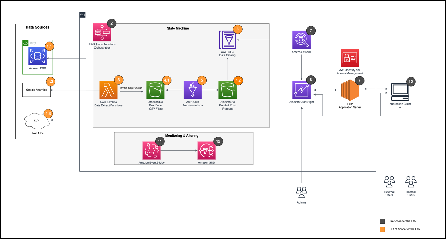
The high-level architecture for integrating Security Lake with OpenSearch Service is as follows.

The workflow contains the following steps:

  1. Security Lake persists Parquet formatted data into an S3 bucket as determined by the administrator of Security Lake.
  2. A notification is placed in Amazon SQS that describes the key to get access to the object.
  3. Java code in an AWS Lambda function reads the SQS notification and prepares to read the object described in the notification.
  4. Java code uses Hadoop, Parquet, and Avro libraries to retrieve the object from Amazon S3 and transform the records in the Parquet object into JSON documents for indexing in your OpenSearch Service domain.
  5. The documents are gathered and then sent to your OpenSearch Service domain, where index templates map the structure into a schema optimized for Security Lake logs in OCSF format.

Steps 1–2 are managed by Security Lake; steps 3–5 are managed by the customer. The shaded components are your responsibility. The subscriber implementation for this solution uses Lambda and OpenSearch Service, and these resources are managed by you.

If you are evaluating this as solution for your business, remember that Lambda has a 15-minute maximum execution time at the time of this writing. Security Lake can produce up to 256MB object sizes and this solution may not be effective for your company’s needs at large scale. Various levers in Lambda have impacts on the cost of the solution for log delivery. Make cost conscious decisions when evaluating sample solutions. This implementation using Lambda is suitable for smaller companies where to volume of logs for CloudTrail and VPC flow logs are more suitable for a Lambda based approach where the cost to transform and deliver logs to Amazon OpenSearch Service are more budget friendly.

Now that you have some context, let’s start building the implementation for OpenSearch Service!

Prerequisites

Creation of Security Lake for your AWS accounts is a prerequisite for building this solution. Security Lake integrates with an AWS Organizations account to enable the offering for selected accounts in the organization. For a single AWS account that doesn’t use Organizations, you can enable Security Lake without the need for Organizations. You must have administrative access to perform these operations. For multiple accounts, it’s suggested that you delegate the Security Lake activities to another account in your organization. For more information about enabling Security Lake in your accounts, review Getting started.

Additionally, you may need to take the provided template and adjust it to your specific environment. The sample solution relies on access to a public S3 bucket hosted for this blog so egress rules and permissions modifications may be required if you use S3 endpoints.

This solution assumes that you’re using a domain deployed in a VPC. Additionally, it assumes that you have fine-grained access controls enabled on the domain to prevent unauthorized access to data you store as part of the integration with Security Lake. VPC-deployed domains are privately routable and have no access to the public internet by design. If you want to access your domain in a more public setting, you need to create a NGINX proxy to broker a request between public and private settings.

The remaining sections in this post are focused on how to create the integration with OpenSearch Service.

Create the subscriber

To create your subscriber, complete the following steps:

  1. On the Security Lake console, choose Subscribers in the navigation pane.
  2. Choose Create subscriber.
  3. Under Subscriber details, enter a meaningful name and description.
  4. Under Log and event sources, specify what the subscriber is authorized to ingest. For this post, we select All log and event sources.
  5. For Data access method, select S3.
  6. Under Subscriber credentials, provide the account ID and an external ID for which AWS account you want to provide access.
  7. For Notification details, select SQS queue.
  8. Choose Create when you are finished filling in the form.

It will take a minute or so to initialize the subscriber framework, such as the SQS integration and the permission generated so that you can access the data from another AWS account. When the status changes from Creating to Created, you have access to the subscriber endpoint on Amazon SQS.

  1. Save the following values found in the subscriber Details section:
    1. AWS role ID
    2. External ID
    3. Subscription endpoint

Use AWS CloudFormation to provision Lambda integration between the two services

An AWS CloudFormation template takes care of a large portion of the setup for the integration. It creates the necessary components to read the data from Security Lake, transform it into JSON, and then index it into your OpenSearch Service domain. The template also provides the necessary AWS Identity and Access Management (IAM) roles for integration, the tooling to create an S3 bucket for the Java JAR file used in the solution by Lambda, and a small Amazon Elastic Compute Cloud (Amazon EC2) instance to facilitate the provisioning of templates in your OpenSearch Service domain.

To deploy your resources, complete the following steps:

  1. On the AWS CloudFormation console, create a new stack.
  2. For Prepare template, select Template is ready.
  3. Specify your template source as Amazon S3 URL.

You can either save the template to your local drive or copy the link for use on the AWS CloudFormation console. In this example, we use the template URL that points to a template stored on Amazon S3. You can either use the URL on Amazon S3 or install it from your device.

  1. Choose Next.
  2. Enter a name for your stack. For this post, we name the stack blog-lambda. Start populating your parameters based on the values you copied from Security Lake and OpenSearch Service. Ensure that the endpoint for the OpenSearch domain has a forward slash / at the end of the URL that you copy from OpenSearch Service.
  3. Populate the parameters with values you have saved or copied from OpenSearch Service and Security Lake, then choose Next.
  4. Select Preserve successfully provisioned resources to preserve the resources in case the stack roles back so you can debug the issues.
  5. Scroll to bottom of page and choose Next.
  6. On the summary page, select the check box that acknowledges IAM resources will be created and used in this template.
  7. Choose Submit.

The stack will take a few minutes to deploy.

  1. After the stack has deployed, navigate to the Outputs tab for the stack you created.
  2. Save the CommandProxyInstanceID for executing scripts and save the two role ARNs to use in the role mappings step.

You need to associate the IAM roles for the tooling instance and the Lambda function with OpenSearch Service security roles so that the processes can work with the cluster and the resources within.

Provision role mappings for integrations with OpenSearch Service

With the template-generated IAM roles, you need to map the roles using role mapping to the predefined all_access role in your OpenSearch Service cluster. You should evaluate your specific use of any roles and ensure they are aligned with your company’s requirements.

  1. In OpenSearch Dashboards, choose Security in the navigation pane.
  2. Choose Roles in the navigation pane and look up the all_access role.
  3. On the role details page, on the Mapped users tab, choose Manage mapping.
  4. Add the two IAM roles found in the outputs of the CloudFormation template, then choose Map.

Provision the index templates used for OCSF format in OpenSearch Service

Index templates have been provided as part of the initial setup. These templates are crucial to the format of the data so that ingestion is efficient and tuned for aggregations and visualizations. Data that comes from Security Lake is transformed into a JSON format, and this format is based directly on the OCSF standard.

For example, each OCSF category has a common Base Event class that contains multiple objects that represent details like the cloud provider in a Cloud object, enrichment data using an Enrichment object that has a common structure across events but can have different values based on the event, and even more complex structures that have inner objects, which themselves have more inner objects such as the Metadata object, still part of the Base Event class. The Base Event class is the foundation for all categories in OCSF and helps you with the effort of correlating events written into Security Lake and analyzed in OpenSearch.

OpenSearch is technically schema-less. You don’t have to define a schema up front. The OpenSearch engine will try to guess the data types and the mappings found in the data coming from Security Lake. This is known as dynamic mapping. The OpenSearch engine also provides you with the option to predefine the data you are indexing. This is known as explicit mapping. Using explicit mappings to identifying your data source types and how they are stored at time of ingestion is key to getting high volume ingest performance for time-centric data indexed at heavy load.

In summary, the mapping templates use composable templates. In this construct, the solution establishes an efficient schema for the OCSF standard and gives you the capability to correlate events and specialize on specific categories in the OCSF standard.

You load the templates using the tools proxy created by your CloudFormation template.

  1. On the stack’s Outputs tab, find the parameter CommandProxyInstanceID.

We use that value to find the instance in AWS Systems Manager.

  1. On the Systems Manager console, choose Fleet manager in the navigation pane.
  2. Locate and select your managed node.
  3. On the Node actions menu, choose Start terminal session.
  4. When you’re connected to the instance, run the following commands:
    cd;pwd
    . /usr/share/es-scripts/es-commands.sh | grep -o '{\"acknowledged\":true}' | wc -l

You should see a final result of 42 occurrences of {“acknowledged”:true}, which demonstrates the commands being sent were successful. Ignore the warnings you see for migration. The warnings don’t affect the scripts and as of this writing can’t be muted.

  1. Navigate to Dev Tools in OpenSearch Dashboards and run the following command:
    GET _cat/templates

This confirms that the scripts were successful.

Install index patterns, visualizations, and dashboards for the solution

For this solution, we prepackaged a few visualizations so that you can make sense of your data. Download the visualizations to your local desktop, then complete the following steps:

  1. In OpenSearch Dashboards, navigate to Stack Management and Saved Objects.
  2. Choose Import.
  3. Choose the file from your local device, select your import options, and choose Import.

You will see numerous objects that you imported. You can use the visualizations after you start importing data.

Enable the Lambda function to start processing events into OpenSearch Service

The final step is to go into the configuration of the Lambda function and enable the triggers so that the data can be read from the subscriber framework in Security Lake. The trigger is currently disabled; you need to enable it and save the config. You will notice the function is throttled, which is by design. You need to have templates in the OpenSearch cluster so that the data indexes in the desired format.

  1. On the Lambda console, navigate to your function.
  2. On the Configurations tab, in the Triggers section, select your SQS trigger and choose Edit.
  3. Select Activate trigger and save the setting.
  4. Choose Edit concurrency.
  5. Configure your concurrency and choose Save.

Enable the function by setting the concurrency setting to 1. You can adjust the setting as needed for your environment.

You can review the Amazon CloudWatch logs on the CloudWatch console to confirm the function is working.

You should see startup messages and other event information that indicates logs are being processed. The provided JAR file is set for information level logging and if needed, to debug any concerns, there is a verbose debug version of the JAR file you can use. Your JAR file options are:

If you choose to deploy the debug version, the verbosity of the code will show some error-level details in the Hadoop libraries. To be clear, Hadoop code will display lots of exceptions in debug mode because it tests environment settings and looks for things that aren’t provisioned in your Lambda environment, like a Hadoop metrics collector. Most of these startup errors are not fatal and can be ignored.

Visualize the data

Now that you have data flowing into OpenSearch Service from Security Lake via Lambda, it’s time to put those imported visualizations to work. In OpenSearch Dashboards, navigate to the Dashboards page.

You will see four primary dashboards aligned around the OCSF category for which they support. The four supported visualization categories are for DNS activity, security findings, network activity, and AWS CloudTrail using the Cloud API.

Security findings

The findings dashboard is a series of high-level summary information that you use for visual inspection of AWS Security Hub findings in a time window specified by you in the dashboard filters. Many of the encapsulated visualizations give “filter on click” capabilities so you can narrow your discoveries. The following screenshot shows an example.

The Finding Velocity visualization shows findings over time based on severity. The Finding Severity visualization shows which “findings” have passed or failed, and the Findings table visualization is a tabular view with actual counts. Your goal is to be near zero in all the categories except informational findings.

Network activity

The network traffic dashboard provides an overview for all your accounts in the organization that are enabled for Security Lake. The following example is monitoring 260 AWS accounts, and this dashboard summarizes the top accounts with network activities. Aggregate traffic, top accounts generating traffic and top accounts with the most activity are found in the first section of the visualizations.

Additionally, the top accounts are summarized by allow and deny actions for connections. In the visualization below, there are fields that you can drill down into other visualizations. Some of these visualizations have links to third party website that may or may not be allowed in your company. You can edit the links in the Saved objects in the Stack Management plugin.

For drill downs, you can drill down by choosing the account ID to get a summary by account. The list of egress and ingress traffic within a single AWS account is sorted by the volume of bytes transferred between any given two IP addresses.

Finally, if you choose the IP addresses, you’ll be redirected to Project Honey Pot, where you can see if the IP address is a threat or not.

DNS activity

The DNS activity dashboard shows you the requestors for DNS queries in your AWS accounts. Again, this is a summary view of all the events in a time window.

The first visualization in the dashboard shows DNS activity in aggregate across the top five active accounts. Of the 260 accounts in this example, four are active. The next visualization breaks the resolves down by the requesting service or host, and the final visualization breaks out the requestors by account, VPC ID, and instance ID for those queries run by your solutions.

API Activity

The final dashboard gives an overview of API activity via CloudTrail across all your accounts. It summarizes things like API call velocity, operations by service, top operations, and other summary information.

If we look at the first visualization in the dashboard, you get an idea of which services are receiving the most requests. You sometimes need to understand where to focus the majority of your threat discovery efforts based on which services may be consumed differently over time. Next, there are heat maps that break down API activity by region and service and you get an idea of what type of API calls are most prevalent in your accounts you are monitoring.

As you scroll down on the form, more details present themselves such as top five services with API activity and the top API operations for the organization you are monitoring.

Conclusion

Security Lake integration with OpenSearch Service is easy to achieve by following the steps outlined in this post. Security Lake data is transformed from Parquet to JSON, making it readable and simple to query. Enable your SecOps teams to identify and investigate potential security threats by analyzing Security Lake data in OpenSearch Service. The provided visualizations and dashboards can help to navigate the data, identify trends and rapidly detect any potential security issues in your organization.

As next steps, we recommend to use the above framework and associated templates that provide you with easy steps to visualize your Security Lake data using OpenSearch Service.

In a series of follow-up posts, we will review the source code and walkthrough published examples of the Lambda ingestion framework in the AWS Samples GitHub repo. The framework can be modified for use in containers to help address companies that have longer processing times for large files published in Security Lake. Additionally, we will discuss how to detect and respond to security events using example implementations that use OpenSearch plugins such as Security Analytics, Alerting, and the Anomaly Detection available in Amazon OpenSearch Service.


About the authors

Kevin Fallis (@AWSCodeWarrior) is an Principal AWS Specialist Search Solutions Architect. His passion at AWS is to help customers leverage the correct mix of AWS services to achieve success for their business goals. His after-work activities include family, DIY projects, carpentry, playing drums, and all things music.

Jimish Shah is a Senior Product Manager at AWS with 15+ years of experience bringing products to market in log analytics, cybersecurity, and IP video streaming. He’s passionate about launching products that offer delightful customer experiences, and solve complex customer problems. In his free time, he enjoys exploring cafes, hiking, and taking long walks

Ross Warren is a Senior Product SA at AWS for Amazon Security Lake based in Northern Virginia. Prior to his work at AWS, Ross’ areas of focus included cyber threat hunting and security operations. When he is not talking about AWS he likes to spend time with his family, bake bread, make sawdust and enjoy time outside.

Optimize queries using dataset parameters in Amazon QuickSight

Post Syndicated from Anwar Ali original https://aws.amazon.com/blogs/big-data/optimize-queries-using-dataset-parameters-in-amazon-quicksight/

Amazon QuickSight powers data-driven organizations with unified business intelligence (BI) at hyperscale. With QuickSight, all users can meet varying analytic needs from the same source of truth through modern interactive dashboards, paginated reports, embedded analytics and natural language queries.

We have introduced dataset parameters, a new kind of parameter in QuickSight that can help you create interactive experiences in your dashboards. In this post, we dive deeper into what dataset parameters are, explain the key differences between dataset and analysis parameters, and discuss different use cases for dataset parameters along their benefits.

Introduction to dataset parameters

Before going deep into dataset parameters, let’s first discuss QuickSight analysis parameters. QuickSight analysis parameters are named variables that can transfer a value for use by an action or an object. Parameters help users create interactive experiences in their dashboards. You can tie parameters with other features in the QuickSight analysis. For example, a dashboard user can reference a parameter value in multiple places, using controls, filters, and actions, and also within calculated fields, narratives, and dynamic titles. Then the visuals in the dashboard react to the user’s selection of parameter value. Parameters can also help connect one dashboard to another, allowing a dashboard user to drill down into data that’s in a different analysis.

Dataset parameters, on the other hand, are defined at the dataset level. With dataset parameters, authors can optimize the experience and load time of dashboards that are connected live to external SQL-based sources. When readers interact with their data, the selection and actions they make in controls, filters, and visuals can be propagated to the data sources via live, custom, parameterized SQL queries. By mapping multiple dataset parameters to analysis parameters, users can create a wide variety of experiences using controls, user actions, parameterized URLs, and calculated fields, as well as dynamic visuals’ titles and insights.

In the following example, dataset owners connected via direct query to a table containing data about taxi rides in New York. They can add a WHERE clause in their custom SQL to filter the dataset based on the end-user’s input of a specific pickup date that will be later provided by the dashboard readers. In the SQL query, the rows are filtered by the date in the dataset parameter <<$pPickupDate>> if it matches the date in the pickupdate column. This way, the dataset size can be significantly smaller for users that are only interested in data for a specific taxi ride date. See the following code:

SELECT *
FROM nytaxidata
WHERE pickupdate = <<$pPickupDate>>

To allow users to provide multiple values in the parameter, you can create a multi-value parameter (for example, pPickupDates), and insert the parameter into an IN phrase as follows:

SELECT *
FROM nytaxidata
WHERE pickupdate in (<<$pPickupDates>>)

Use cases for dataset parameters

In this section, we discuss common use cases using dataset parameters and their benefits.

Optimized custom SQL in direct queries

With dataset parameters, you no longer have to trade-off between the flexibility of using custom SQL logic and the performance of an optimized SQL query. Parameterized datasets can be filtered to a relatively smaller result set when loaded. Authors and readers can benefit from the faster load of analyses and dashboards for the first time using default values, as well as for later queries when data is sliced and diced using filter controls on the dashboard. Also, data owners benefit from their datasets putting less load on backend database resources, making it more scalable and performant to serve higher user concurrency.

The performance gains will be evident when you work with direct query datasets that have complex custom SQL, such as nested queries that have to filter the data in the inner sections of the query.

Generic datasets reusable across analyses

Dataset parameters can enable datasets to be largely reused across various analyses, thereby reducing the effort for the data owners to prepare and maintain the datasets. Whether you have a SPICE dataset or direct query dataset, with dataset parameters, you can port calculated field referencing parameters from the analysis to the dataset. Authors can now reuse calculated fields referencing parameters created by dataset owners in a dataset, rather than recreate these fields across multiple analysis.

With the option to port parameter-dependent calculated fields from the analysis to the underlying datasets, dataset parameters can help you create the same calculated fields in the dataset and reuse them across multiple analyses. This is important for governance use cases as well: dataset owners can move the parameter-dependent calculated fields from the analysis to protect the business logic, ensuring that their calculated fields can’t be modified by analyses’ authors.

Simpler dataset maintenance with repeatable variables

When you have a dataset that refers to a static value (placeholder) in multiple places in custom SQL and calculated fields, you can now create a dataset parameter and reuse it in multiple places. This will help in better code maintainability. (Note that inserting parameters in custom SQL is only available in direct query.)

Solution overview

In this scenario, we create a custom SQL direct query dataset to observe unoptimized SQL queries that are generated without dataset parameters, and demonstrate how your current custom SQL queries run if you don’t use dataset parameters. Then we modify the custom SQL, add the dataset parameter, and show the optimized query generated for the same dataset if we use dataset parameters.

In this example, we use an Amazon RDS for PostgreSQL database. However, this feature will work with any SQL-based data source in QuickSight.

Query your data with analysis parameters

To set up your data source, dataset, and analysis, complete the following steps. If you’re using real data, you can skip to the next section.

  1. Create a QuickSight data source.

The following screenshot shows sample connection details.

create a datasource

  1. Create a new direct query custom SQL dataset.

We are using sample data from NYC OpenData for New York taxi rides with a subset of approximately 1 million records. The data is loaded in an RDS for PostgreSQL database table called nytaxidata.

create a sample dataset nytaxidata

  1. Create a sample analysis using the dataset you just created. Choose the table visual and add a few columns from the Fields list.

create a sample analysis using nytaxidata dataset

  1. Reload the analysis and observe the query generated on the PostgreSQL database.

You will notice it loads the full dataset (select * from nytaxidata) as referenced in the screenshot below from RDS Performance Insight.

SQL from performance insight, unoptimized SQL inner query without where clause

  1. Add an analysis parameter-based filter control to the QuickSight analysis. Change the value of this filter control (analysis parameter in this case).

creating analysis parameter with a control

The inner query over the dataset still uses custom SQL without using the filter in the WHERE clause. This filter control parameter is still part of the WHERE clause of the outer query, so the custom SQL fetches the complete result set as part of the inner query. This may not be the case if you use database tables as a dataset rather than a custom SQL query as a dataset. With a dataset based directly on tables, parameter values are passed to the database in the WHERE clause.

SQL from performance insight, unoptimized SQL inner query without where clause with analysis parameter

So how do we overcome the challenge of being able to include the parameter in the WHERE clause in custom SQL datasets? With dataset parameters!

Optimize your query with dataset parameters

Let’s look at a few scenarios where we can use dataset parameters to send more optimized queries to the database.

  1. Create a dataset parameter (for example, pDSfareamount) and add it to the WHERE clause with an equality predicate in the custom SQL.Observe if there is any change in the SQL query that was passed to the database.

creating dataset parameter

This time, you will see optimized SQL generated using the default parameter value in the WHERE clause of the inner query (select * from nytaxidata where fare_amount=0). This results in better query performance for direct query datasets.

optimized sql generated with dataset parameter

Map dataset parameters with analysis parameters

Dataset parameters can be mapped to analysis parameters and user-selected values can pass to the dataset parameters from the interactions on the dashboard at run time.

You can use a single analysis parameter and map it to multiple dataset parameters. The parent analysis parameter can now be linked with a filter control or an action, and can help you filter multiple datasets based on custom SQL.

In this section, we map a dataset parameter with an analysis parameter and bind it with a filter control at runtime.

  1. First, we create an analysis parameter and map it to a dataset parameter (we use the dataset parameter we created earlier).

mapping analysis parameter with a dataset parameter

  1. Now the analysis parameter (for this example, pAfareamount) is created. You can create the control object Fare Amount to dynamically change the dataset parameter value from the analysis or dashboard using a parameter control. You can bind pAfareamount with a QuickSight filter to pass values to the dataset parameter dynamically. When you’re changing values in a parameter control, you will find optimized SQL on the backend database with the WHERE predicate in inner query generated.

chaing value of analysis parameter mapped to dataste parameter via filter control

Additional examples using dataset parameters

So far, we have used dataset parameters with an equality predicate.Let’s look at a few more scenarios using dataset parameters.

  1. The following screenshot demonstrates using a dataset parameter with a range predicate of custom SQL.

dataset parameter with non equality predicate

  1. The following example illustrates using two dataset parameters with a between operator.

two dataset parameters with between operator

  1. The following example shows using a dataset parameter within a calculation.

dataset parameter used in calculated field based on ifelse condition

  1. We can also use a dataset parameter with a scalar user-defined function (UDF). In the following example, we have a scalar function is_holiday(pickupdate), which takes a pickupdate as a parameter and returns a flag of 0 or 1 based on whether pickupdate is a public holiday.

dataset parameter used with scalar user defined function

  1. Additionally, we can use a dataset parameter to derive a calculated field. In the following example, we need to calculate the surcharge_amount dynamically based on a value specified at runtime and the number of passengers. We use a dataset parameter along with a case statement to calculate the desired surcharge_amount.

dataset paramter with calculated field case statement

  1. The final example illustrates how to move calculations using parameters in the analysis to the dataset for reusability.

porting dataset parameter from analysis to dataset

Dataset parameter limitations

The following are the known limitations (as of this writing) that you may encounter when working with dataset parameters in QuickSight:

  • Dataset parameters can’t be inserted into custom SQL of datasets stored in SPICE.
  • Dynamic defaults can only be configured on the analysis page of the analysis that is using the dataset. You can’t configure a dynamic default at the dataset level.
  • The Select all option is not supported on multi-value controls of analysis parameters that are mapped to dataset parameters (but there is a workaround that you can follow).
  • Cascading controls are not supported for dataset parameters.
  • Dataset parameters can only be used by dataset filters when the dataset is using a direct query.
  • When dashboard readers schedule emailed reports, selected controls don’t propagate to the dataset parameters that are included in the report that is attached to the email. Instead, the default values of the parameters are used.

Refer to Using dataset parameters in Amazon QuickSight for more information.

Conclusion

In this post, we showed you how to create QuickSight dataset parameters and map them to analysis parameters. Dataset parameters help improve your QuickSight dashboard performance for direct query custom SQL datasets by generating optimized SQL queries. We also showed a few examples of how to use dataset parameters in SQL range predicates, calculated fields, scalar UDFs, and case statements.

Dataset parameters enable dataset owners to centrally create and govern parameter-dependent calculated fields at the dataset level. Such calculated fields can be reused across multiple analyses, and cannot be tampered with by analysis authors.

We hope you will find dataset parameters in QuickSight useful. We have already seen how the feature is creatively used in a wide range of use cases. We recommend that you review your existing direct query custom SQL datasets in your QuickSight deployment to look for candidates for optimization, or take advantage of the other benefits of dataset parameters. For example, BI teams can benefit from dataset parameters by reusing the same dataset with different values in the parameter to analyze different slices of the same data, such as different regions, products, or customers by industry segments.

Are you considering migrating legacy reports to QuickSight? Dataset parameters can help enterprise BI developers reduce the migration effort of legacy reports that already have parameterized SQL queries in the legacy queries. These SQL queries can be passed along their parameters to QuickSight datasets via automations with the help of QuickSight APIs (and a few adjustments to the queries if the parameters are marked differently).

For more information on dataset parameters, refer to Using dataset parameters in Amazon QuickSight.


About the authors

Anwar Ali is a Specialist Solutions Architect for Amazon QuickSight. Anwar has over 18 years of experience implementing enterprise business intelligence (BI), data analytics and database solutions . He specializes in integration of BI solutions with business applications, helping customers in BI architecture design patterns and best practices.

Salim Khan is a Specialist Solutions Architect for Amazon QuickSight. Salim has over 16 years of experience implementing enterprise business intelligence (BI) solutions. Prior to AWS, Salim worked as a BI consultant catering to industry verticals like Automotive, Healthcare, Entertainment, Consumer, Publishing and Financial Services. He has delivered business intelligence, data warehousing, data integration and master data management solutions across enterprises.

Gil Raviv is a Principal Product Manager for Amazon QuickSight, AWS’ cloud-native, fully managed SaaS BI service. As a thought-leader in BI, Gil accelerated the growth of global BI practices at AWS and Avanade, and has guided Fortune 1000 enterprises in their Data & AI journey. As a passionate evangelist, author and blogger of low-code/no-code data prep and analytic tools, Gil was awarded 5 times as a Microsoft MVP (Most Valuable Professional).

Efficiently crawl your data lake and improve data access with an AWS Glue crawler using partition indexes

Post Syndicated from Srividya Parthasarathy original https://aws.amazon.com/blogs/big-data/efficiently-crawl-your-data-lake-and-improve-data-access-with-aws-glue-crawler-using-partition-indexes/

In today’s world, customers manage vast amounts of data in their Amazon Simple Storage Service (Amazon S3) data lakes, which requires convoluted data pipelines to continuously understand the changes in the data layout and make them available to consuming systems. AWS Glue crawlers provide a straightforward way to catalog data in the AWS Glue Data Catalog that removes the heavy lifting when it comes to schema management and data classification. AWS Glue crawlers extract the data schema and partitions from Amazon S3 to automatically populate the Data Catalog, keeping the metadata current.

But with data growing exponentially over time, the number of partitions in a given table can grow significantly. Because analytics services like Amazon Athena query a table containing millions of partitions, the time needed to retrieve the partition increases and can cause query runtime to increase.

Today, AWS Glue crawler support has been expanded to automatically add partition indexes for newly discovered tables to optimize query processing on the partitioned dataset. Now, when the crawler creates a new Data Catalog table during a crawler run, it also creates a partition index by default, with the largest permutation of all numeric and string type partition columns as keys. The Data Catalog then creates a searchable index based on these keys, reducing the time required to retrieve and filter partition metadata on tables with millions of partitions. The creation of partition indexes benefits the analytics workloads running on Athena, Amazon EMR, Amazon Redshift Spectrum, and AWS Glue.

In this post, we describe how to create partition indexes with an AWS Glue crawler and compare the query performance improvement when accessing the crawled data with and without a partition index from Athena.

Solution overview

We use an AWS CloudFormation template to create our solution resources. In the following steps, we demonstrate how to configure the AWS Glue crawler to create a partition index using either the AWS Glue console or the AWS Command Line Interface (AWS CLI). Then we compare the query performance improvements using Athena.

Prerequisites

To follow along with this post, you must have access to an AWS Identity and Access Management (IAM) administrator role to create resources using AWS CloudFormation.

Set up your solution resources

The CloudFormation template generates the following resources:

  • IAM roles and policies
  • An AWS Glue database to hold the schema
  • An AWS Glue crawler pointing to a highly partitioned dataset
  • An Athena workgroup and bucket to store query results

Complete the following steps to set up the solution resources:

  1. Log in to the AWS Management Console as an IAM administrator.
  2. Choose Launch Stack to deploy the CloudFormation template:
  3. For DatabaseName, keep the default blog_partition_index_crawlerdb.
  4. Choose Next.
  5. Review the details on the final page and select I acknowledge that AWS CloudFormation might create IAM resources.
  6. Choose Create stack.
  7. When the stack is complete, on the AWS CloudFormation console, navigate to the Outputs tab of the stack.
  8. Note down values of DatabaseName and GlueCrawlerName.

Some of the resources that this stack deploys incur costs when in use.

Edit and run the AWS Glue crawler

To configure and run the AWS Glue crawler, complete the following steps:

  1. On the AWS Glue console, choose Crawlers in the navigation pane.
  2. Locate the crawler blog-partition-index-crawler and choose Edit.
  3. In the Set output and scheduling section, under Advanced options, select Create partition indexes automatically.
  4. Review and update the crawler settings.

Alternatively, you can configure your crawler using the AWS CLI (provide your IAM role and Region):

aws glue create-crawler --name blog-partition-index-crawler --targets '{ "S3Targets": [{ "Path": "s3://awsglue-datasets/examples/highly-partitioned-table/"}] }' --database-name "blog_partition_index_crawlerdb" --role <Crawler_IAM_role> --configuration "{\"Version\":1.0,\"CreatePartitionIndex\":true}" --region <region_name>
  1. Now run the crawler and verify that the crawler run is complete.

This is highly partitioned dataset and will take approximately 90 minutes to complete.

Verify the partitioned table

In the AWS Glue database blog_partition_index_crawlerdb, verify that the table highly_partitioned_table is created.

By default, the crawler determines an index based on the largest permutation of partition columns of valid column types in the same order of partition columns, which are either numeric or string. For the table created by the crawler (highly_partitioned_table), we have partition columns year (string), month (string), day (string), and hour (string).

Based on this definition, the crawler created an index on the permutation of year, month, day, and hour. The crawler created the indexes prefixed with crawler_ on any partition index created by default.

Verify the same by navigating to the table highly_partitioned_table on the AWS Glue console and choosing the Indexes tab.

The crawler was able to crawl the S3 data source and successfully populate the partition indexes for the table.

Compare the query performance improvements using Athena

First, we query the table in Athena without using the partition index. To verify the tables using Athena, complete the following steps:

  1. On the Athena console, choose crawler-primary-workgroup as the Athena workgroup and choose Acknowledge.
  2. Run the following query:
    select count(*), sum(value) from blog_partition_index_crawlerdb.highly_partitioned_table where year='1980' and month='01' and day ='01'

The following screenshot shows the query took approximately 32 seconds without filtering enabled using the partition index.

  1. Now we enable the partition index on the Athena query:
    ALTER TABLE blog_partition_index_crawlerdb.highly_partitioned_table
    SET TBLPROPERTIES ('partition_filtering.enabled' = 'true')

  2. Run the following query again and note the runtime:
    select count(*), sum(value) from blog_partition_index_crawlerdb.highly_partitioned_table where year=‘1980’ and month=‘01’ and day =‘01’

The following screenshot shows the query took only 700 milliseconds, which is much faster with filtering enabled using the partition index.

Clean up

To avoid unwanted charges to your AWS account, you can delete the AWS resources:

  1. Sign in to the CloudFormation console as the IAM admin used for creating the CloudFormation stack.
  2. Delete the CloudFormation stack you created.

Conclusion

In this post, we explained how to configure an AWS crawler to create partition indexes and compared the query performance when accessing the data with indexes from Athena.

If no partition indexes are present on the table, AWS Glue loads all the partitions of the table, and then filters the loaded partitions, which results in inefficient retrieval of metadata. Analytics services like Redshift Spectrum, Amazon EMR, and AWS Glue ETL Spark DataFrames can now utilize indexes for fetching partitions, resulting in significant query performance.

For more information on partition indexes and query performance across various analytical engines, refer to Improve Amazon Athena query performance using AWS Glue Data Catalog partition indexes and Improve query performance using AWS Glue partition indexes.

Special thanks to everyone who contributed to this crawler feature launch: Yuhang Chen, Kyle Duong,and Mita Gavade.


About the authors

Srividya Parthasarathy is a Senior Big Data Architect on the AWS Lake Formation team. She enjoys building data mesh solutions and sharing them with the community.

Sandeep Adwankar is a Senior Technical Product Manager at AWS. Based in the California Bay Area, he works with customers around the globe to translate business and technical requirements into products that enable customers to improve how they manage, secure, and access data.

Enable data collaboration among public health agencies with AWS Clean Rooms – Part 1

Post Syndicated from Venkata Kampana original https://aws.amazon.com/blogs/big-data/part-1-enable-data-collaboration-among-public-health-agencies-with-aws-clean-rooms/

In this post, we show how you can use AWS Clean Rooms to enable data collaboration between public health agencies. Public health governmental agencies need to understand trends related to a variety of health conditions and care across populations in order to create policies and treatments with the goal of improving the well-being of the various communities they serve.

In order to do this, these agencies need to analyze data from many sources, such as clinical organizations, non-clinical community organizations, and administrative data from other government agencies, so they can identify trends around health conditions and treatments across populations. Public health needs to understand what is happening to populations within the communities they serve.

Because they are looking at populations at risk, they need the flexibility of a line list of cases, stripped of personally identifiable information (PII). With this information, they can assess risk based on a variety of demographic and social factors available in the data sources without divulging PII. The list gives them flexibility to apply more complex analyses, such as regression, on the linked data as well. Programs like MENDS, MDPHnet, and CODI have explored using clinical data in distributed networks to understand the burden of chronic diseases in communities for years. Challenges facing these programs include complex data sharing rules and distributed analytics approaches, across networks of data providers. MENDS and MDPHnet, for example, run analytics at the organization level without deduplicating across sites. Individual queries are pushed to each site where they are processed and reviewed by humans, and combined output is sent to the public health agency.

AWS Clean Rooms offers an opportunity to reduce the burden on data providers in programs like these, while enabling public health agencies to analyze data using their own queries and mitigate risks to data privacy by preventing access to the underlying raw data.

Overview of AWS Clean Rooms

AWS Clean Rooms was first announced at AWS re:Invent 2022, and is now generally available. AWS Clean Rooms allows customers and their partners to more easily and securely collaborate on their collective datasets—without sharing or copying the underlying data with each other. AWS Clean Rooms provides a broad set of privacy-enhancing controls that help protect sensitive data, including query controls, query output restrictions, query logging, and cryptographic computing tools.

With AWS Clean Rooms, you can collaborate and analyze data with other parties in the collaboration without either party having to share or copy the raw data. AWS Clean Rooms is a stateless service; it doesn’t store the data. Instead, it reads the data from where it lives, applies restrictions that protect each participant’s underlying data at query runtime, and returns the results. Queries can be written to intersect and analyze data sources using common metadata elements (for example, geography, shared identifiers, or other demographic factors), generating row-level lists of the overlap between the data sources or aggregated counts by population, condition, or other strata.

AWS Clean Rooms helps public health agencies analyze collective data to gain a more complete view of the health and well-being of their communities, while maintaining the security and privacy of the data.

Solution overview

Before we get started with AWS Clean Rooms, let’s first talk about some of the service’s key concepts:

  • Collaborations – This is a secure logical boundary in AWS Clean Rooms created by the collaboration creator. When creating the collaboration, the creator can invite additional members to join the collaboration. Invited participants can see the list of collaboration members before they accept the invitation to join the collaboration.
  • Members – This refers to AWS customers who are participants in a collaboration. All collaboration members can join data; however, only one member can query and receive results per collaboration, and that member is immutable.
  • Analysis rules – AWS Clean Rooms supports two types of analysis rules:
    • Aggregation – Members can run queries that aggregate statistics using COUNT, SUM, or AVG functions along optional dimensions. Aggregation queries won’t reveal row-level data.
    • List – Members can run queries that output row-level data of the overlap between two tables.
  • Configured tables – Members can configure existing AWS Glue tables for use in AWS Clean Rooms. This data is stored in Amazon Simple Storage Service (Amazon S3) in open data formats and cataloged in the AWS Glue Data Catalog. Each configured table contains an analysis rule that determines how the data can be queried. After it’s configured, members can associate the configured table to one or more collaborations.

Getting started with AWS Clean Rooms is a four-step process:

  1. The creator configures a collaboration and invites one or more members to the collaboration.
  2. The invited member joins the collaboration.
  3. Members can configure the existing AWS Glue tables for use in AWS Clean Rooms.
  4. Members with permission to do so can run queries in the collaboration.

Prerequisites

For this walkthrough, you need the following:

Create a collaboration and invite one or more members

You must define your collaboration configuration on the AWS Clean Rooms console, via the AWS Command Line Interface (AWS CLI), or with an AWS SDK. We demonstrate how to configure this on the console.

  1. On the AWS Clean Rooms console, choose Create collaboration.

  2. For Name, enter a name (for example, Demo collaboration).
  3. For Description, add an optional description.
  4. In the Members section, add the following members:
    1. Member 1 – Enter a member display name (your AWS account ID is automatically populated).
    2. Member 2 – Enter a member display name and the AWS account ID for the member you want to invite.
    3. Choose Add another member to add more members.
  5. In the Member abilities section, choose one member who will query and receive results.
  6. In the Query logging section, select Support query logging for this collaboration to log the queries in Amazon CloudWatch logs.
  7. Choose Next.
  8. In the Collaboration membership section, select the storage option you prefer for CloudWatch.
  9. Choose Next.
  10. On the Review and create page, choose Create collaboration and membership after reviewing the details to ensure accuracy.

Congratulations on creating your first collaboration! You can see the collaboration details on the Collaborations page.

Join the collaboration

Each collaboration member can log in to AWS Clean Rooms console, review the invitation, and decide to join the collaboration by following these steps:

  1. On the AWS Clean Rooms console, choose Collaborations in the navigation pane.
  2. On the Available to join tab, choose the collaboration you were invited to.

On the details page, you can review the member abilities.

  1. Select your preferred log storage option and choose Create membership.
  2. On the confirmation page, verify that the members listed align with your data sharing agreements, then choose Create membership.

After you create your membership, your member status is changed to Active on the collaboration dashboard.

Configure existing AWS Glue tables for use in AWS Clean Rooms

AWS Clean Rooms doesn’t require you to make a copy of the data because it reads the data from Amazon S3. This eliminates the need to copy and load your data into destinations outside your respective AWS account, or use third-party services to facilitate data sharing.

Each collaboration member can create configured tables, an AWS Clean Rooms resource that contains reference to the AWS Glue Data Catalog with underlying data that defines how that data can be used. The configured table can be used across many collaborations.

  1. On the AWS Clean Rooms console, choose Configured tables in the navigation pane.
  2. Choose Configure new table.
  3. Choose the database to populate the list of AWS Glue tables, and choose the table you want to associate with the collaboration.

For each selected table, you can determine which columns can be accessed in the collaboration.

  1. Select All columns or select Custom list to choose a subset of columns to be available in the collaboration.
  2. Enter a name for the configured table.
  3. Choose Configure new table.

In addition to column-level access controls, AWS Clean Rooms provides fine-grained query controls called analysis rules. With built-in and flexible analysis rules, you can tailor queries to specific business needs. As discussed earlier, AWS Clean Rooms provides two types of analysis rules:

  • Aggregation analysis rules – These allow queries that aggregate data without revealing row-level information. Available functions include COUNT, SUM, and AVG, along optional dimensions.
  • List analysis rules – These allow queries that output row-level attribute analyses of the overlap between the tables in the collaboration space.

Both rule types allow data owners to mandate a join between their datasets and the datasets of the collaborator running the query. This limits the results to just their intersection of the collaborators datasets.

  1. On the configured table, choose Configure analysis rule to configure the analysis rules.
  2. For this post, we select List because we want to query patients’ immunization status by joining with immunization data from other contributors.
  3. Select the creation method and select Next.
  4. To define the criteria for the table joins, in the Join controls section, choose the column names appropriate for the join.
  5. To specify which columns will be outputted, identify those in the List controls section.
  6. Choose Next.
  7. Choose Configure analysis rule on the Review and configure page.

You will see the message Successfully configured list analysis rule on the configured tables page.

  1. Choose Associate to collaboration to link this table to the collaboration you created.
  2. Review the details on the Associate table page and choose Associate table.

The collaboration page will display a list of tables that are associated by you to the collaboration.

Each member of the collaboration must repeat the aforementioned steps to associate their AWS Glue Data Catalog tables to the collaboration. For this post, the other members of the collaboration follow these same steps to associate their data to the collaboration. Then the collaboration will list all tables associated by other members.

After defining the analysis rules on the configured tables and associating them to the collaboration, the members who can query and receive results can start writing queries according to the restrictions defined by each participating collaboration member. The following section includes example collaboration queries.

Run queries in the collaboration

The following screenshot is an example of a query that won’t be successful because * is not supported. Column names must be specified in the query.

The following screenshot is an example of a query that won’t be successful because you can’t link columns that members restricted in your joins.

The following screenshot is an example of a query that will be successful because it uses permitted columns (columns that are part of the list analysis rule) in the select clause and join condition.

The sample datasets (Patient and Immunization) used in this post include a unique identifier (patient ID). However, in a real-world scenario, this might not be the case. In those situations, you may consider using privacy-preserving record linkage (PPRL) to create a unique deidentified token. For example, the CDC’s CODI program deduplicates across data owners by obfuscating PII behind each organization’s firewall in a standardized way. That obfuscated information is joined to create a unique deidentified token for each individual that is analyzed across data sources. If public health agencies want to conduct analyses based on individually linked longitudinal data, they could apply PPRL to each data source and use that metadata element to link the data sources in AWS Clean Rooms before conducting their analytics.

Clean up

As part of this walkthrough, you provisioned an AWS Clean Rooms collaboration, invited other members to join the collaboration, and configured tables. To delete these resources, refer to Leaving the collaboration and Disassociating configured tables.

Conclusion

In this post, we showed you how to create a collaboration, invite other members to the collaboration, configure existing AWS Glue Catalog tables, apply analysis rules, and run sample queries on the AWS Clean Rooms console. In Part 2 of this series, we demonstrate how to automate query runs using AWS Lambda, query the results using Amazon Athena, and publish dashboards using Amazon QuickSight.


About the Authors

Venkata Kampana is a Senior Solutions Architect in the AWS Health and Human Services team and is based in Sacramento, CA. In that role, he helps public sector customers achieve their mission objectives with well-architected solutions on AWS.

Dr. Dawn Heisey-Grove is the public health analytics leader for Amazon Web Services’ state and local government team. In this role, she’s responsible for helping state and local public health agencies think creatively about how to achieve their analytics challenges and long-term goals. She’s spent her career finding new ways to use existing or new data to support public health surveillance and research.

Jim Daniel is the Public Health lead at Amazon Web Services. Previously, he held positions with the United States Department of Health and Human Services for nearly a decade, including Director of Public Health Innovation and Public Health Coordinator. Before his government service, Jim served as the Chief Information Officer for the Massachusetts Department of Public Health.

Improved resiliency with backpressure and admission control for Amazon OpenSearch Service

Post Syndicated from Ketan Verma original https://aws.amazon.com/blogs/big-data/improved-resiliency-with-backpressure-and-admission-control-for-amazon-opensearch-service/

Amazon OpenSearch Service is a managed service that makes it simple to secure, deploy, and operate OpenSearch clusters at scale in the AWS Cloud. Last year, we introduced Shard Indexing Backpressure and admission control, which monitors cluster resources and incoming traffic to selectively reject requests that would otherwise pose stability risks like out of memory and impact cluster performance due to memory contentions, CPU saturation and GC overhead, and more.

We are now excited to introduce Search Backpressure and CPU-based admission control for OpenSearch Service, which further enhances the resiliency of clusters. These improvements are available for all OpenSearch versions 1.3 or higher.

Search Backpressure

Backpressure prevents a system from being overwhelmed with work. It does so by controlling the traffic rate or by shedding excessive load in order to prevent crashes and data loss, improve performance, and avoid total failure of the system.

Search Backpressure is a mechanism to identify and cancel in-flight resource-intensive search requests when a node is under duress. It’s effective against search workloads with anomalously high resource usage (such as complex queries, slow queries, many hits, or heavy aggregations), which could otherwise cause node crashes and impact the cluster’s health.

Search Backpressure is built on top of the task resource tracking framework, which provides an easy-to-use API to monitor each task’s resource usage. Search Backpressure uses a background thread that periodically measures the node’s resource usage and assigns a cancellation score to each in-flight search task based on factors like CPU time, heap allocations, and elapsed time. A higher cancellation score corresponds to a more resource-intensive search request. Search requests are cancelled in descending order of their cancellation score to recover nodes quickly, but the number of cancellations is rate-limited to avoid wasteful work.

The following diagram illustrates the Search Backpressure workflow.

Search requests return an HTTP 429 “Too Many Requests” status code upon cancellation. OpenSearch returns partial results if only some shards fail and partial results are allowed. See the following code:

{
    "error": {
        "root_cause": [
            {
                "type": "task_cancelled_exception",
                "reason": "cancelled task with reason: heap usage exceeded [403mb >= 77.6mb], elapsed time exceeded [1.7m >= 45s]"
            }
        ],
        "type": "search_phase_execution_exception",
        "reason": "SearchTask was cancelled",
        "phase": "fetch",
        "grouped": true,
        "failed_shards": [
            {
                "shard": 0,
                "index": "nyc_taxis",
                "node": "9gB3PDp6Speu61KvOheDXA",
                "reason": {
                    "type": "task_cancelled_exception",
                    "reason": "cancelled task with reason: heap usage exceeded [403mb >= 77.6mb], elapsed time exceeded [1.7m >= 45s]"
                }
            }
        ],
        "caused_by": {
            "type": "task_cancelled_exception",
            "reason": "cancelled task with reason: heap usage exceeded [403mb >= 77.6mb], elapsed time exceeded [1.7m >= 45s]"
        }
    },
    "status": 429
}

Monitoring Search Backpressure

You can monitor the detailed Search Backpressure state using the node stats API:

curl -X GET "https://{endpoint}/_nodes/stats/search_backpressure"

You can also view the cluster-wide summary of cancellations using Amazon CloudWatch. The following metrics are now available in the ES/OpenSearchService namespace:

  • SearchTaskCancelled – The number of coordinator node cancellations
  • SearchShardTaskCancelled – The number of data node cancellations

The following screenshot shows an example of tracking these metrics on the CloudWatch console.

CPU-based admission control

Admission control is a gatekeeping mechanism that proactively limits the number of requests to a node based on its current capacity, both for organic increases and spikes in traffic.

In addition to the JVM memory pressure and request size thresholds, it now also monitors each node’s rolling average CPU usage to reject incoming _search and _bulk requests. It prevents nodes from being overwhelmed with too many requests leading to hot spots, performance problems, request timeouts, and other cascading failures. Excessive requests return an HTTP 429 “Too Many Requests” status code upon rejection.

Handling HTTP 429 errors

You’ll receive HTTP 429 errors if you send excessive traffic to a node. It indicates either insufficient cluster resources, resource-intensive search requests, or an unintended spike in the workload.

Search Backpressure provides the reason for rejection, which can help fine-tune resource-intensive search requests. For traffic spikes, we recommend client-side retries with exponential backoff and jitter.

You can also follow these troubleshooting guides to debug excessive rejections:

Conclusion

Search Backpressure is a reactive mechanism to shed excessive load, while admission control is a proactive mechanism to limit the number of requests to a node beyond its capacity. Both work in tandem to improve the overall resiliency of an OpenSearch cluster.

Search Backpressure is available in OpenSearch, and we are always looking for external contributions. You can refer to the RFC to get started.


About the authors

Ketan Verma is a Senior SDE working on Amazon OpenSearch Service. He is passionate about building large-scale distributed systems, improving performance, and simplifying complex ideas with simple abstractions. Outside work, he likes to read and improve his home barista skills.

Suresh N S is a Senior SDE working on Amazon OpenSearch Service. He is passionate towards solving problems in large scale distributed systems.

Pritkumar Ladani is an SDE-2 working on Amazon OpenSearch Service. He likes to contribute to open source software development, and is passionate about distributed systems. He is an amateur badminton player and enjoys trekking.

Bukhtawar Khan is a Principal Engineer working on Amazon OpenSearch Service. He is interested in building distributed and autonomous systems. He is a maintainer and an active contributor to OpenSearch.

AWS Professional Services scales by improving performance and democratizing data with Amazon QuickSight

Post Syndicated from Ameya Agavekar original https://aws.amazon.com/blogs/big-data/aws-professional-services-scales-by-improving-performance-and-democratizing-data-with-amazon-quicksight/

The AWS Professional Services (ProServe) Insights team builds global operational data products that serve over 8,000 users within Amazon. Our team was formed in 2019 as an informal group of four analysts who supported ad hoc analysis for a division of ProServe consultants. ProServe is responsible for assisting enterprises as they shift to the cloud by incorporating Amazon Web Services (AWS) into their overall architecture. In recent years, the demand for domain expertise (ProServe) grew as various industries and organizations accelerated the move to the cloud.

We work hand in hand with customer teams and AWS partners to provide deep expertise in the architecture, design, development, and implementation of cloud computing initiatives that result in real business outcomes.

As our organization grew rapidly, we built new tools to scale analytical insights into our customers’ sales and delivery mechanisms. We were frustrated by the limitations of our previous business intelligence (BI) solution, which was holding us back from our vision to accelerate data sharing, team collaboration, and security within Amazon. To scale and continue innovating, we developed a secure Amazon QuickSight environment for our internal customers.

In this post, we discuss how QuickSight has helped us improve our performance, democratize our data, and provide insights to our internal customers at scale.

Enabling teams to build their own analyses at scale

The Insights team builds dashboards and supports thousands of internal consultants and hundreds of analysts and engineers across the globe who drive local products and insights. As a team of engineers focused on building a single source of truth within Amazon, we wanted a BI tool that was cost-effective, secure, and integrated seamlessly with the other AWS services we use. ProServe team members need to make strategic decisions on behalf of customers, and we play a key role by providing the tools they need to make the right decisions. We’ve made a big impact with QuickSight because it doesn’t require in-depth knowledge about data visualizations to build dashboards and provide insights, empowering our users to build what they need.

Our QuickSight instance is secure and tailored to use the Amazon active directory framework. We also helped 13 Amazon teams to set up their own instances. The teams we serve have benefited from our switch to QuickSight. For example, AWS Professional Services launched Financial Insights Tool (FIT) 2 years ago, a QuickSight dashboard that reports project financials, project revenue leakage, and margin erosion by evaluating actuals and forecasts at any granularity. FIT saves 30 minutes per project per Engagement Manager (EM) per week, and securely centralizes project financials into a scalable tool. This empowers EMs to avoid building disparate local reporting that creates logic inconsistencies and data security issues.

One of our ProServe teams has 19 dashboards on QuickSight, including Catalog, Trend and Analysis, KPI Monitoring, Business Management, and Quality Control. In 2022, one of the KPI Monitoring dashboards helped save at least 5,600 hours in total across 230 managers and 2,000 consultants. Last year, this team also reported over 29,600 distinct views on their 19 dashboards.

Additionally, we launched the first iteration of a hygiene dashboard in February 2022. This dashboard helps our operations team and end customers improve the data quality of key attribution and reduce manual intervention. The hygiene dashboard makes sure all the checks are enabled to safely promote customer outcomes with better planning and forecasting capabilities. The adoption of the dashboard led to a 73% reduction in hygiene issues from February 2022 to February 2023. We attribute this reduction to better inspection from weekly business reviews, and with this dashboard as an inspection tool delivered via email subscription to our stakeholders.

Improved performance and flexibility

To onboard a new reader or author on our previous BI tool, we had to provide a new license each time. This manual process was time-consuming and costly. The QuickSight usage-based pricing model makes sure that we can provide analytics and insights to all users without the need to pay ahead for user-specific licenses. QuickSight guarantees that we can provide everyone access by default, enabling data democratization in ways we couldn’t before. Since moving to QuickSight, we have scaled from 1,400 licenses to over 8,000 unique viewers, thanks to its auto scaling capability. QuickSight is fully managed, serverless, and can automatically scale to tens of thousands of users without any infrastructure to manage or capacity to plan for.

We used to have to track our dashboard loading times on our previous tool, but QuickSight has made that a thing of the past. With QuickSight SPICE (Super-fast, Parallel, In-memory Calculation Engine), our dashboards load in seconds, not minutes. Our high impact dashboards for ProServe weekly business reviews, utilization and time card deep dive, and impact points use the powerful SPICE functionality, which has support for up to 1 billion rows.

The Weekly Business Review (WBR) Backlog Summary dashboard that replaced the complex scorecards with interactive QuickSight visuals:

Implementing the FAIRS data sharing framework

QuickSight improves the ability to securely Find, Access, Interoperate, and Reuse (FAIRS) the data across ProServe, AWS, and Amazon. This framework can be described as follows:

  • Findable – Metadata and data should be easy to find for both humans and computers. All datasets and dashboards in the same account provide us an opportunity to see the big picture. This streamlines the reports’ and dashboards’ dictionary-building process for ProServe. Automatic discovery of datasets, reports, and dashboards improves the analytical community’s efficiency and productivity.
  • Accessible – Users need to be able to access the data they need easily and securely. In our case, we can control the access using appropriate roles, groups, and highly secure authentication methods not only for users but also for our data sources, datasets, and dashboards using Amazon Active Directory Connected Groups.
  • Interoperable – As the worldwide central team across 10 geographies and over 2,000 practices, our data needs to interoperate with applications or workflows for analysis, storage, and processing. This allows many different parts of the organization to collaborate as a cohesive unit.
  • Reusable – The ultimate goal of FAIRS is to optimize the reuse of data. To achieve this, metadata and data should be well-described so that they can be replicated or combined in different settings. This way, we can save time and focus our analysis on diving deeper into the insights.
  • Security – Security is job Zero. We believe that everyone should have secure data access to make data-driven decisions. At ProServe, we use Amazon Active Directory, column-level security (CLS), and row-level security (RLS) to maintain the high bar in data security.

QuickSight has brought us closer to achieving FAIRS than we could get with our previous BI solution. Dashboards are easily searchable, highly collaborative, and secure.

The User Activities Tracking dashboard created by ProServe’s QuickSight administrators:

Seamless AWS Integration

QuickSight integrates seamlessly with other AWS services such as Amazon SageMaker to use machine learning insights within a low code or no code environment. Our users can simply connect to any of the QuickSight supported data sources—including Amazon Simple Storage Service (Amazon S3), Amazon Athena, Amazon Relational Database Service (Amazon RDS), and Amazon Redshift—and select the SageMaker model they want to use for prediction. QuickSight has also made it possible for dashboard development from non-analyst roles.

QuickSight is constantly evolving. Eighty-four features were added in 2022. One of those features is asset management, which has made it easier for us to transfer assets from one group to another to onboard new employees. With QuickSight, we have reached over 9,200 distinct viewers and over 500,000 total views at Amazon with 485 dashboards.

The Skills dashboard representing the percentage match of top 100 skills entered by each specialization:

QuickSight has enabled us to scale with the growth of our team without sacrificing our performance. Instead, we improved our performance and democratized our data, thanks to great capabilities such as SPICE, the flexibility of the product, and its seamless integration with the other AWS services. We look forward to continuing to provide solutions to our internal customers by exploring other QuickSight capabilities such as Amazon QuickSight Q, embedded analytics, and more.

To learn more about how QuickSight can help your business with dashboards, reports, and more, visit Amazon QuickSight.


About the Authors

Ameya Agavekar is a results-driven, highly skilled data strategist. Ameya leads the data engineering and data science function for AWS Professional Services World-Wide Business Insights & Analytics team. Outside of work, Ameya is a professional pilot. He enjoys serving community by applying his unique flying skills with the US Airforce auxiliary Civil Air Patrol.

Tucker Shouse leads the AWS Professional Services World-Wide Business Insights & Analytics team. Prior to AWS, Tucker worked with financial services, retail, healthcare, and non-profit clients to develop digital and data products and strategies as a Manager at Alvarez & Marsal Corporate Performance Improvement. Outside of work, Tucker enjoys spending time with his wife and daughter enjoying the outdoors and music.

Best practices for running production workloads using Amazon MSK tiered storage

Post Syndicated from Nagarjuna Koduru original https://aws.amazon.com/blogs/big-data/best-practices-for-running-production-workloads-using-amazon-msk-tiered-storage/

In the second post of the series, we discussed some core concepts of the Amazon Managed Streaming for Apache Kafka (Amazon MSK) tiered storage feature and explained how read and write operations work in a tiered storage enabled cluster.

This post focuses on how to properly size your MSK tiered storage cluster, which metrics to monitor, and the best practices to consider when running a production workload.

Sizing a tiered storage cluster

Sizing and capacity planning are critical aspects of designing and operating a distributed system. It involves estimating the resources required to handle the expected workload and ensure the system can scale and perform efficiently. In the context of a distributed system like Kafka, sizing involves determining the number of brokers, the number of partitions, and the amount of storage and memory required for each broker. Capacity planning involves estimating the expected workload, including the number of producers, consumers, and the throughput requirements.

Let’s assume a scenario where the producers are evenly balancing the load between brokers, brokers host the same number of partitions, there are enough partitions to ingest the throughput, and consumers consume directly from the tip of the stream. The brokers are receiving the same load and doing the same work. We therefore just focus on Broker1 in the following diagram of a data flow within a cluster.

Theoretical sustained throughput with tiered storage

We derive the following formula for the theoretical sustained throughput limit tcluster given the infrastructure characteristics of a specific cluster with tiered storage enabled on all topics:

max(tcluster) <= min {

max(tstorage) * #brokers/(r + 1 + #non_tip_local_consumer_groups),
max(tNetworkAttachedStorage) * #brokers/(r + 1 + #non_tip_local_consumer_groups),
max(tEC2network) * #brokers/(#tip_consumer_groups + r + #remote_consumer_groups)

}

This formula contains the following values:

  • tCluster – Total ingress produce throughput sent to the cluster
  • tStorage – Storage volume throughput supported
  • tNetworkAttachedStorage – Network attached storage to the Amazon Elastic Compute Cloud (Amazon EC2) instance network throughput
  • tEC2network – EC2 instance network bandwidth
  • non_tip_local_consumer_groups – Number of consumer groups reading from network attached storage at ingress rate
  • tip_consumer_groups – Number of consumer groups reading from page cache at ingress rate
  • remote_consumer_groups – Number of consumer groups reading from remote tier at ingress rate
  • r – Replication factor of the Kafka topic

Note that in the first post , we didn’t differentiate between different types of consumer groups. With tiered storage, some consumer groups might be consuming from remote. These remote consumers might ultimately catch up and start reading from local storage and finally catch up to the tip. Therefore, we model these three different consumer groups in the equation to account for their impact on infrastructure usage. In the following sections, we provide derivations of this equation.

Derivation of throughput limit from network attached storage bottleneck

Because Amazon MSK uses network attached storage for local storage, both network attached storage throughput and bandwidth should be accounted for. Total throughput bandwidth requirement is a combination of ingress and egress from the network attached storage backend. The ingress throughput of the storage backend depends on the data that producers are sending directly to the broker plus the replication traffic the broker is receiving from its peers. With tiered storage, Amazon MSK also uses network attached storage to read and upload rolled segments to the remote tier. This doesn’t come from the page cache and needs to be accounted for at the rate of ingress. Any non-tip consumers at ingress rate also consume network attached storage throughput and are accounted for in the equation. Therefore, max throughput is bounded by network attached storage based on the following equation:

max(tcluster) <= min {

max(tstorage) * #brokers/(r + 1 + #non_tip_local_consumer_groups),
max(tNetworkAttachedStorage) * #brokers/(r + 1 + #non_tip_local_consumer_groups)

}

Derivation of throughput limit from EC2 network bottleneck

Unlike network attached storage, the network is full duplex, meaning that if the EC2 instance supports X MB/s network, it supports X MB/s in and X MB/s out. The network throughput requirement depends on the data that producers are sending directly to the broker plus the replication traffic the broker is receiving from its peers. It also includes the replication traffic out and consumers traffic out from this broker. With tiered storage, we need to reserve additional ingress rate for uploads to the remote tier and support reads from the remote tier for consumer groups reading from remote offset. Both of these add to the network out requirements, which is bounded by the following equation:

max(tcluster) <= min {

max(tEC2network) * #brokers/(#tip_consumer_groups + r + #remote_consumer_groups)

}

Combining the second and third equations provides the first formula, which determines the max throughput bound based on broker infrastructure limits.

How to apply this formula to size your cluster

With this formula, you can calculate the upper bound for throughput you can achieve for your workloads. In practice, the workloads may be bottlenecked by other broker resources like CPU, memory, and disk, so it’s important to do load tests. To simplify your sizing estimate, you can use the MSK Sizing and Pricing spreadsheet (for more information, refer to Best Practices).

Let’s consider a workload where your ingress and egress rates are 20MB/s, with a replication factor of 3, and you want to retain data in your Kafka cluster for 7 days. This workload requires 6x m5.large brokers, with 34.6 TB local storage, which will cost $6,034.00 monthly (estimated). But if you use tiered storage for the same workload with local retention of 4 hours and overall data retention of 7 days, it requires 3x m5.large brokers, with 0.8 TB local storage and 12 TB of tiered storage, which will cost $1,958.00 monthly(estimated). If you want to read all the historic data one time, it will cost $17.00 ($0.0015 per GB retrieval cost). In this example with tiered storage, you save around 67.6% of your overall cost.

We recommend planning for Availability Zone redundancy in production workloads considering the broker safety factor in the calculation, which is 1 in this example. We also recommend running performance tests to ensure CPU is less than 70% on your brokers at the target throughput derived based on this formula or Excel calculation. In addition, you should also use the per-broker partition limit in your calculation to account for other bottlenecks based on the partition count.

The following figure shows an example of Amazon MSK sizing.

Monitoring and continuous optimization for a tiered storage enabled cluster

In previous sections, we emphasized the importance of determining the correct initial cluster size. However, it’s essential to recognize that sizing efforts shouldn’t cease after the initial setup. Continual monitoring and evaluation of your workload are necessary to ensure that the broker size remains appropriate. Amazon MSK offers metric monitoring and alarm capabilities to provide visibility into cluster performance. In the post Best practices for right-sizing your Apache Kafka clusters to optimize performance and cost, we discussed key metrics to focus on. In this post, we delve deeper into additional metrics related to tiered storage and other optimization considerations for a tiered storage enabled cluster:

  • TotalTierBytesLag indicates the total number of bytes of the data that is eligible for tiering on the broker and hasn’t been transferred to the tiered storage yet. This metric shows the efficiency of upstream data transfer. As the lag increases, the amount of data that hasn’t yet persisted in the tiered storage increases. The impact is the network attached storage disk may fill up, which you should monitor. You should also monitor this metric and generate an alarm if the lag is continuously growing and you see increased network attached storage usage. If the tiering lag is too high, you can reduce ingress traffic to allow the tiered storage to catch up.
  • Although tiered storage provides on-demand, virtually unlimited storage capacity without provisioning any additional resources, you should still do proper capacity planning for your local storage, configure alerts for KafkaDataLogsDiskUsed metrics, and have a buffer on network attached storage capacity planning. Monitor this metric and generate an alarm if the metric reaches or exceeds 60%. For a tiered storage enabled topic, configure local retention accordingly to reduce network attached storage usage.
  • The theoretical max ingress we can achieve on an MSK cluster with tiered storage is 20–25% lower than a non-tiered storage enabled cluster due to additional network attached storage bandwidth required to transparently move data from the local to the remote tier. Plan for the capacity (brokers, storage, gp2 vs. gp3) using the formula we discussed to derive max ingress for your cluster based on the number of consumer groups and load test your workloads to identify the sustained throughput limit. Exercising excess ingress to the cluster or egress from the remote tier above the planned capacity can impact your tip produce or consume traffic.
  • The gp3 volume type offers SSD-performance at a 20% lower cost per GB than gp2 volumes. Furthermore, by decoupling storage performance from capacity, you can easily provision higher IOPS and throughput without the need to provision additional block storage capacity. Therefore, we recommend using gp3 for a tiered storage enabled cluster by specifying provisioned throughput for larger instance types.
  • If you specified a custom cluster configuration, check the num.replica.fetchers, num.io.threads, and num.network.threads configuration parameters on your cluster. We recommend leaving it as the default Amazon MSK configuration unless you have specific use case.

This is only the most relevant guidance related to tiered storage. For further guidance on monitoring and best practices of your cluster, refer to Best practices.

Conclusion

You should now have a solid understanding of how Amazon MSK tiered storage works and the best practices to consider for your production workload when utilizing this cost-effective storage tier. With tiered storage, we remove the compute and storage coupling, which can benefit workloads that need larger disk capacity and are underutilizing compute just to provision storage.

We are eager to learn about your current approach in building real-time data streaming applications. If you’re starting your journey with Amazon MSK tiered storage, we suggest following the comprehensive Getting Started guide available in Tiered storage. This guide provides detailed instructions and practical steps to help you gain hands-on experience and effectively take advantage of the benefits of tiered storage for your streaming applications.

If you have any questions or feedback, please leave them in the comments section.


About the authors

Nagarjuna Koduru is a Principal Engineer in AWS, currently working for AWS Managed Streaming For Kafka (MSK). He led the teams that built MSK Serverless and MSK Tiered storage products. He previously led the team in Amazon JustWalkOut (JWO) that is responsible for realtime tracking of shopper locations in the store. He played pivotal role in scaling the stateful stream processing infrastructure to support larger store formats and reducing the overall cost of the system. He has keen interest in stream processing, messaging and distributed storage infrastructure.

Masudur Rahaman Sayem is a Streaming Data Architect at AWS. He works with AWS customers globally to design and build data streaming architectures to solve real-world business problems. He specializes in optimizing solutions that use streaming data services and NoSQL. Sayem is very passionate about distributed computing.

How Klarna Bank AB built real-time decision-making with Amazon Kinesis Data Analytics for Apache Flink

Post Syndicated from Nir Tsruya original https://aws.amazon.com/blogs/big-data/how-klarna-bank-ab-built-real-time-decision-making-with-amazon-kinesis-data-analytics-for-apache-flink/

This is a joint post co-authored with Nir Tsruya from Klarna Bank AB.

Klarna is a leading global payments and shopping service, providing smarter and more flexible shopping and purchase experiences to 150 million active consumers across more than 500,000 merchants in 45 countries. Klarna offers direct payments, pay after delivery options, and instalment plans in a smooth one-click purchase experience that lets consumers pay when and how they prefer to. The ability to utilize data to make near-real-time decisions is a source of competitive advantage for Klarna.

This post presents a reference architecture for real-time queries and decision-making on AWS using Amazon Kinesis Data Analytics for Apache Flink. In addition, we explain why the Klarna Decision Tooling team selected Kinesis Data Analytics for Apache Flink for their first real-time decision query service. We show how Klarna uses Kinesis Data Analytics for Apache Flink as part of an end-to-end solution including Amazon DynamoDB and Apache Kafka to process real-time decision-making.

AWS offers a rich set of services that you can use to realize real-time insights. These services include Kinesis Data Analytics for Apache Flink, the solution Klarna that uses to underpin automated decision-making in their business today. Kinesis Data Analytics for Apache Flink allows you to easily build stream processing applications for a variety of sources including Amazon Kinesis Data Streams, Amazon Managed Streaming for Apache Kafka (Amazon MSK), and Amazon MQ.

The challenge: Real-time decision-making at scale

Klarna’s customers expect a real-time, frictionless, online experience when shopping and paying online. In the background, Klarna needs to assess risks such as credit risk, fraud attempts, and money laundering for every customer credit request in every operating geography. The outcome of this risk assessment is called a decision. Decisions generate millions of risk assessment transactions a day that must be run in near-real time. The final decision is the record of whether Klarna has approved or rejected the request to extend credit to a consumer. These underwriting decisions are critical artefacts. First, they contain information that must be persisted for legal reasons. Second, they are used to build profiles and models that are fed into underwriting policies to improve the decision process. Under the hood, a decision is the sum of a number of transactions (for example, credit checks), coordinated and persisted via a decision store.

Klarna wanted to build a framework to ensure decisions persist successfully, ensuring timely risk assessment and quick decisions for customers. First, the Klarna team looked to solve the problem of producing and capturing decisions by using a combination of Apache Kafka and AWS Lambda. By publishing decision artefacts directly to a Kafka topic, the Klarna team found that high latency could cause long transaction wait times or transactions to be rejected altogether, leading to delays in getting ratified decisions to customers in a timely fashion and potential lost revenue. This approach also caused operational overhead for the Klarna team, including management of the schema evolution, replaying old events, and native integration of Lambda with their self-managed Apache Kafka clusters.

Design requirements

Klarna was able to set out their requirements for a solution to capture risk assessment artefacts (decisions), acting as a source of truth for all underwriting decisions within Klarna. The key requirements included at-least once reliability and millisecond latency, enabling real-time access to decision-making and the ability to replay past events in case of missing data in downstream systems. Additionally, the team needed a system that could scale to keep pace with Klarna’s rapid [10 times] growth.

Solution overview

The solution consists of two components: a combination of an highly available API with DynamoDB as the data store to store each decision, and Amazon DynamoDB Streams with Kinesis Data Analytics. Kinesis Data Analytics is a fully managed Apache Flink service and used to stream, process, enrich, and standardize the decision in real time and replay past events (if needed).

The following diagram illustrates the overall flow from end-user to the downstream systems.

The flow includes the following steps:

  1. As the end-user makes a purchase, the policy components assess risk and the decision is sent to a decision store via the Decision Store API.
  2. The Decision Store API persists the data in DynamoDB and responds to the requester. Decisions for each transaction are time-ordered and streamed by DynamoDB Streams. Decision Store also enables centralised schema management and handles evolution of event schemas.
  3. The Kinesis Data Analytics for Apache Flink application is the consumer of DynamoDB streams. The application makes sure that the decisions captured are conforming to the expected event schema that is then published to a Kafka topic to be consumed by various downstream systems. Here, Kinesis Data Analytics for Apache Flink plays a vital part in the delivery of those events: aggregating, enriching, and mapping data to adhere to the event schema. This provides a standardized way for consumers to access decisions from their respective producers. The application enables at-least once delivery capability, and Flink’s checkpoint and retry mechanism guarantees that every event is processed and persisted.
  4. The published Kafka events are consumed by the downstream systems and stored in an Amazon Simple Storage Service (Amazon S3) bucket. The events stored in Amazon S3 reflect every decision ever taken by the producing policy components, and can be used by the decision store to backfill and replay any past events. In addition to preserving the history of decision events, events are also stored as a set of variables in the variable store.
  5. Policy components use the variable store to check for similar past decisions to determine if a request can be accepted or denied immediately. The request is then processed as described by the preceding workflow, and the next subsequent request will be answered by the variable store based on the result of the previous decision.

The decision store provides a standardized workflow for processing and producing events for downstream systems and customer support. With all the events captured and safely stored in DynamoDB, the decision store provides an API for support engineers (and other supporting tools like chatbots) to query and access past decisions in near-real time.

Solution impact

The solution provided benefits in three areas.

First, the managed nature of Kinesis Data Analytics allowed the Klarna team to focus on value-adding application development instead of managing infrastructure. The team is able to onboard new use cases in less than a week. They can take full advantage of the auto scaling feature in Kinesis Data Analytics and pre-built sources and destinations.

Second, the team can use Apache Flink to ensure the accuracy, completeness, consistency, and reliability of data. Flink’s native capability of stateful computation and data accuracy through the use of checkpoints and savepoints directly supports Klarna team’s vision to add more logic into the pipelines, allowing the team to expand to different use cases confidently. Additionally, the low latency of the service ensures that enriched decision artefacts are available to consumers and subsequently to the policy agents for future decision-making in near-real time.

Third, the solution enables the Klarna team to take advantage of the Apache Flink open-source community, which provides rich community support and the opportunity to contribute back to the community by bug fixing or adding new features.

This solution has proven to scale with increased adoption of a new use case, translating to a 10-times increase in events over 3 months.

Lessons learned

The Klarna team faced a few challenges with Flink serialization and upgrading Apache Flink versions. Flink serialization is an interesting concept and critical for the application’s performance. Flink uses a different set of serializers in order to serialize data between the operators. It’s up to the team to configure the best and most efficient serializer based on the use case. The Klarna team configured the objects as Flink POJO, which reduced the pipeline runtime by 85%. For more information, refer to Flink Serialization Tuning Vol. 1: Choosing your Serializer — if you can before deploying a Flink application to production.

The other challenge faced by the team was upgrading the Apache Flink version in Kinesis Data Analytics. Presently, the Kinesis Data Analytics for Apache Flink application requires the creation of a new Kinesis Data Analytics for Apache Flink application. Currently, reusing a snapshot (the binary artefact representing the state of the Flink application, used to restore the application to the last checkpoint taken) is not possible between two different applications. For that reason, upgrading the Apache Flink version requires additional steps in order to ensure the application doesn’t lose data.

What’s next for Klarna and Kinesis Data Analytics for Apache Flink?

The team is looking into expanding the usage of Kinesis Data Analytics and Flink in Klarna. Because the team is already highly experienced in the technology, their first ambition will be to own the infrastructure of a Kinesis Data Analytics for Apache Flink deployment, and connect it to different Klarna data sources. The team then will host business logic provided by other departments in Klarna such as Fraud Prevention. This will allow the specialised teams to concentrate on the business logic and fraud detection algorithms, while decision tooling will handle the infrastructure.

What next Overview

Klarna, AWS, and the Flink community

A key part of choosing Kinesis Data Analytics for Apache Flink was the open-source community and support.

Several teams within Klarna created different implementations of a Flink DynamoDB connector, which were used internally by multiple teams. Klarna then identified the opportunity to create a single maintained DynamoDB Flink connector and contribute it to the open-source community. This has initiated a collaboration within Klarna, led by the Klarna Flink experts and accompanied by Flink open-source contributors from AWS.

The main principle for designing the DynamoDB Flink connector was utilizing the different write capacity modes of DynamoDB. DynamoDB supports On-demand and Provisioned capacity modes and each behaves differently when it comes to how it handles incoming throughput. On-demand mode will automatically scale up DynamoDB write capacity and apply itself to the incoming load. However, Provisioned mode is more limiting, and will throttle incoming traffic according to the provisioned write capacity.

To comply with this process, the DynamoDB Flink connector was designed to allow concurrent writes to DynamoDB. The number of concurrent requests can be configured to comply with DynamoDB’s capacity mode. In addition, the DynamoDB Flink connector supports backpressure handling in case the DynamoDB write provisioning is low compared to the incoming load from the Apache Flink application.

At the time of writing, the DynamoDB Flink connector has been open sourced.

Conclusion

Klarna has successfully been running Kinesis Data Analytics for Apache Flink in production since October 2020. It provides several key benefits. The Klarna development team can focus on development, not on cluster and operational management. Their applications can be quickly modified and uploaded. The low latency properties of the service ensure a near-real-time experience for end-users, data consumers, and producers, which underpin risk assessment and the decision-making processes underpinning continuous traffic growth. At the same time, exactly-once processing in combination with Flink checkpoints and savepoints means that critical decision-making and legal data is not lost.

To learn more about Kinesis Data Analytics and getting started, refer to Using a Studio notebook with Kinesis Data Analytics for Apache Flink and More Kinesis Data Analytics Solutions on GitHub.


About the authors

Nir Tsruya is a Lead Engineer in Klarna. He leads 2 engineering teams focusing mainly on real time data processing and analytics at large scale.

Ankit Gupta is a Senior Solutions Architect at Amazon Web Serves based in Stockholm, Sweden, where we helps customers across the Nordics succeed in Cloud. He’s particularly passionate about building strong Networking foundation in Cloud.

Daniel Arenhage is a Solutions Architect at Amazon Web Services based in Gothenburg, Sweden.

AWS Week in Review – Automate DLQ Redrive for SQS, Lambda Supports Ruby 3.2, and More – June 12, 2023

Post Syndicated from Marcia Villalba original https://aws.amazon.com/blogs/aws/aws-week-in-review-automate-dlq-redrive-for-sqs-lambda-supports-ruby-3-2-and-more-june-12-2023/

Today I’m boarding a plane for Madrid. I will attend the AWS Summit Madrid this Thursday, and I will take Serverlesspresso with me. Serverlesspresso is a demo that we take to events, in where you can learn how to build event-driven architectures with serverless. If you are visiting an AWS Summit, most probably you will find one of our booths.

Serverlesspresso at Madrid

Last Week’s Launches
Here are some launches that got my attention during the previous week.

Amazon SQS – Customers were very excited when we announced the DLQ redrive for Amazon SQS as that feature helped them to easily redirect the failed messages. This week we added support for AWS SDK and CLI for this feature, allowing you to redrive the messages on the DLQ automatically, making it even easier to use this feature. You can read Seb’s blog post about this new feature to learn how to get started.

AWS Lambda – AWS Lambda now supports Ruby 3.2. Ruby 3.2 has many new improvements, for example, passing anonymous arguments to functions or having endless methods. Check out this blog post that goes in depth into each of the new features.

Amazon Fraud DetectorAmazon Fraud Detector supports event orchestration with Amazon EventBridge. This is a very important feature because now you can act on the different events that Fraud Detector emits, for example, send notifications to different stakeholders.

AWS Glue – This week, AWS Glue made two important announcements. First, it announced the general availability of AWS Glue for Ray, a new data integration engine option for AWS Glue. Ray is a popular new open-source compute framework that helps developers to scale their Python workloads. In addition, AWS Glue announced AWS Glue Data Quality, a new capability that automatically measures and monitors data lake and data pipeline quality.

Amazon Elastic Container Registry (Amazon ECR)AWS Signer and Amazon ECR announced a new feature that allows you to sign and verify container images. You can use Signer to validate that only container images you have approved are deployed in your Amazon Elastic Kubernetes Service (Amazon EKS) clusters.

Amazon QuickSightAmazon QuickSight now supports APIs to automate asset deployment, so you can replicate the same QuickSight assets in multiple Regions and account easily. You can read more on how to use those APIs in this blog post.

For a full list of AWS announcements, be sure to keep an eye on the What’s New at AWS page.

Other AWS News
Some other updates and news that you may have missed:

Upcoming AWS Events
Check your calendars and sign up for these AWS events:

  • AWS Silicon Innovation Day (June 21) – A one-day virtual event that focuses on AWS Silicon and how you can take advantage of AWS’s unique offerings. Learn more and register here.
  • AWS Global Summits – There are many summits going on right now around the world: Toronto (June 14), Madrid (June 15), and Milano (June 22).
  • AWS Community Day – Join a community-led conference run by AWS user group leaders in your region: Chicago (June 15), Manila (June 29–30), Chile (July 1), and Munich (September 14).
  • CDK Day CDK Day is happening again this year on September 29. The call for papers for this event is open, and this year we are also accepting talks in Spanish. Submit your talk here.

That’s all for this week. Check back next Monday for another Week in Review!

This post is part of our Week in Review series. Check back each week for a quick roundup of interesting news and announcements from AWS!

— Marcia

Improve table readability and identify outliers with data bars in Amazon QuickSight

Post Syndicated from Bhupinder Chadha original https://aws.amazon.com/blogs/big-data/improve-table-readability-and-identify-outliers-with-data-bars-in-amazon-quicksight/

Amazon QuickSight is a scalable, serverless, machine learning (ML)-powered business intelligence (BI) solution that makes it simple to connect to your data, create interactive dashboards, get access to ML-enabled insights, enable natural language querying of your data, and share visuals and dashboards with tens of thousands of internal and external users, either within QuickSight itself or embedded into any application.

Recently, we launched some new features for tables and pivot tables in QuickSight centered around interactivity and performance. These new features enabled users to alter field visibility, load tables faster, and build consistency across different interactions. In the continuous streak of providing rich user experiences and readability, QuickSight is now introducing data bars for table visual.

In this post, we demonstrate how to use data bars to improve table readability and identify outliers.

Introduction to data bars

Tables are a popular way of organizing and presenting data, but it could be difficult for reading and understanding data, especially in large datasets. One way to make table presentation effective is to provide a visual representation with data bars.

Data bars are essentially bar charts displayed for a given column, where the length of the bar represents each cell value relative to the range of values within the same column. Data bars are very efficient in enabling user focus on outliers and emerging data patterns or trends, especially when dealing with large volumes of data. Data bars improve the readability and navigation of complex tables by integrating tabular data with visualizations. Their visual nature enables quick comprehension and understanding, making them a popular choice for displaying and analyzing data. With QuickSight, you can now use data bars on numeric fields and adjust your color scheme for both positive and negative values individually.

Solution overview

Our use case focuses on AnyHealth Inc., a large hospital corporation in the US. They manage different hospitals across different regions of the country. As part of their analytics requirements, they want to be able to quickly find outliers and determine health economics outcomes. They use QuickSight for their visualizations. With the recent addition of data bars to the available table visuals, AnyHealth can get these insights with ease. Not only that, they can also get the information by reading through the cells. With data bars, they are instantly able to identify the outliers visually, identify values that significantly deviate from rest of the data, and monitor emerging trends. With data bars, understanding and reading the tables has been a breeze.

In the following sections, we examine two use cases using data bars in QuickSight.

Identify outliers with data bars visually

To add a table visual to the analysis with data bars, we create a table visual with at least one metric in the Values field well. In this example, we create a table to load profits across various hospitals and categories. The following screenshot shows our initial data.

Complete the following steps to configure a visualization:

  1. On the table visual, choose the pencil icon to open the Format visual navigation pane.
  2. In the navigation pane, expand the Visuals drop-down menu and choose ADD DATA BARS.
  3. For Value field, choose Profit. By default, data bars are configured for two colors: green for positive values and red for negative values.

Note: Data bars are applicable only on the Values field of the visual.

  1. To further configure these colors, choose the paint bucket icon and choose your preferred color.
  2. Close the Data bars menu.

The data bars visualization now appears in the table and an instant outlier can be identified at South Hospital in Ante/Post Partum category.

Display various metrics on the same scale

AnyHealth often has several metrics that they want to visualize and compare side by side, sliced by a single dimension on a same metric scale. For this use case, they want to visualize revenue, profit, and price sliced by the Hospital dimension. Having all these metrics on the same scale is challenging because the numbers vary greatly. With data bars, AnyHealth was able to achieve this in a very simple and clean way, which enabled them to show their data without additional calculations.

The following screenshot shows the example implementation.

Conclusion

In this post, we looked at the data bars feature in QuickSight, its various use cases, and how to configure them. With data bars, you can analyze and quickly scan a table to see the values of a cell. Furthermore, you can use data bars to identify outliers visually that deviate from the rest of the data. Data bars can be very powerful when it comes to understanding and reading data in tables. Start using data bars to enrich your dashboards’ current visualization and unlock new business use cases today!

If you have any questions or feedback, please leave a comment.

For additional discussions and help getting answers to your questions, check out the QuickSight Community.


About the authors

Bhupinder Chadha is a senior product manager for Amazon QuickSight focused on visualization and front end experiences. He is passionate about BI, data visualization and low-code/no-code experiences. Prior to QuickSight he was the lead product manager for Inforiver, responsible for building a enterprise BI product from ground up. Bhupinder started his career in presales, followed by a small gig in consulting and then PM for xViz, an add on visualization product.

Raji Sivasubramaniam is a Sr. Solutions Architect at AWS, focusing on Analytics. Raji is specialized in architecting end-to-end Enterprise Data Management, Business Intelligence and Analytics solutions for Fortune 500 and Fortune 100 companies across the globe. She has in-depth experience in integrated healthcare data and analytics with wide variety of healthcare datasets including managed market, physician targeting and patient analytics.

Srikanth Baheti is a Specialized World Wide Principal Solution Architect for Amazon QuickSight. He started his career as a consultant and worked for multiple private and government organizations. Later he worked for PerkinElmer Health and Sciences & eResearch Technology Inc, where he was responsible for designing and developing high traffic web applications, highly scalable and maintainable data pipelines for reporting platforms using AWS services and Serverless computing.

Joulica unifies real-time and historical customer experience analytics with Amazon QuickSight

Post Syndicated from Tony McCormack original https://aws.amazon.com/blogs/big-data/joulica-unifies-real-time-and-historical-customer-experience-analytics-with-amazon-quicksight/

This is a guest post by Tony McCormack from Joulica.

Joulica is an Ireland-based startup in the contact center industry. Our founders previously led contact center research and development for a global contact center technology provider, and we founded Joulica because we saw that the shift to the cloud and growing demand for data and analytics would transform the customer service industry. Our platform delivers real-time and historical analytics across the wide variety of data sources and customer interaction channels that are now common in most organizations.

It is our mission to make customer experience analytics accessible to all users in an organization. Our customers need to have instant access to the current state of ongoing customer engagements as well trends and historical data patterns. They find it difficult to harness all of the data sources needed to achieve this, particularly in real time. To help solve this problem, we chose Amazon QuickSight, a cloud-native business intelligence tool that allows you to embed insightful analytics into any application with customized, interactive visuals and dashboards.

In this post, we discuss how QuickSight has allowed us to achieve our goal of unifying real-time and historical analytics for our customers.

Embedding QuickSight to provide a 360-degree view

At Joulica, our specialty is real-time analytics. Real-time analytics means that as soon as new data is available, analytics are updated, including any visualizations that are currently being viewed by end-users. The rich embedding capability of QuickSight allowed us to use QuickSight for historical analytics and our technology for real-time analytics, all in one place. Visual embedding with QuickSight has saved us greater than two resource years of research and development time, enabling us to serve customers sooner. We have also been able integrate Joulica real-time analytics into QuickSight dashboards—so within QuickSight, our users can use both standard QuickSight visualizations and Joulica widgets, as shown in the following example.

Our customer journey analytics go beyond typical contact center reporting, and stitches together how customers interact with organizations across channels. By pushing our analytics to QuickSight, we allow users to dive deep into patterns as well as individual customer journeys.

Integration with Amazon Connect and other AWS services

One of the main reasons we chose QuickSight was because of its alignment with Amazon Connect and the extended set of Contact Center services that AWS provides. As the leading provider of analytics for Amazon Connect, this was essential. We are deeply integrated with the full capabilities of Amazon Connect, including Amazon Lex and Contact Lens. In the preceding example of a QuickSight dashboard, we see that as soon as a KPI is updated, the visualization automatically updates. Behind the scenes, Joulica is ingesting Agent Event Streams, Contact Events, and a host of real-time data feeds from Amazon Connect, analyzing them and pushing a stream of real-time analytics to these widgets. This enables our customers to have up-to-date information, in addition to the historical context, empowering them to improve contact center performance and make better decisions. This is all visualized within QuickSight.

We can also ingest data from Amazon Kinesis and Apache Kafka, allowing live analytics from additional data sources to be visualized.

Empowering our customers with insights in QuickSight

The key goals driving the need for analytics in the contact center industry are customer experience optimization as well as efficiency gains. This is relevant across all customer touchpoints, including digital channels, traditional contact center channels, and emerging areas such as social and smart devices. In addition to KPIs related to service levels and agent performance, organizations need access to customer feedback and sentiment analytics, as well as an explanation of how these are related to business performance such as sales and customer retention. With QuickSight, we can offer out-of-the box analytics for all of these areas. The following example shows how easy it is to use the Quicksight visual embedding feature to extend one of our real-time visualizations to show a geographic breakdown of customer survey results.

Thanks to the QuickSight and AWS pay-as-you-go pricing model, we can provide real-time and historical embedded analytics to our customers automatically. We have saved significantly by choosing QuickSight, both in cost and development time, and the cost savings provided by Quicksight is passed down to our customers. Like AWS, our pricing is usage-based, meaning that our customers can scale as their operations grow.

We currently have customers in North America, United Kingdom, the EU, and APAC. As we continue to grow, we plan to explore other QuickSight features like Amazon QuickSight Q, as we pursue providing more ways for our customers to analyze, visualize, and interpret their contact center data.

To learn more about how you can embed customized data visuals and interactive dashboards into any application, visit Amazon QuickSight Embedded. To learn more about Joulica, please visit Joulica.io.


About the Author

Tony McCormack is the CEO and Co-founder of Joulica. Based in Galway, Ireland, he is focused on providing enterprise-grade reporting and analytics for Amazon Connect, Salesforce Service Cloud, and other platforms in the customer experience market. He has extensive experience in the contact center domain, with a passion for real-time analytics and their integration into end-user applications.

Choosing an open table format for your transactional data lake on AWS

Post Syndicated from Shana Schipers original https://aws.amazon.com/blogs/big-data/choosing-an-open-table-format-for-your-transactional-data-lake-on-aws/

A modern data architecture enables companies to ingest virtually any type of data through automated pipelines into a data lake, which provides highly durable and cost-effective object storage at petabyte or exabyte scale. This data is then projected into analytics services such as data warehouses, search systems, stream processors, query editors, notebooks, and machine learning (ML) models through direct access, real-time, and batch workflows. Data in customers’ data lakes is used to fulfil a multitude of use cases, from real-time fraud detection for financial services companies, inventory and real-time marketing campaigns for retailers, or flight and hotel room availability for the hospitality industry. Across all use cases, permissions, data governance, and data protection are table stakes, and customers require a high level of control over data security, encryption, and lifecycle management.

This post shows how open-source transactional table formats (or open table formats) can help you solve advanced use cases around performance, cost, governance, and privacy in your data lakes. We also provide insights into the features and capabilities of the most common open table formats available to support various use cases.

You can use this post for guidance when looking to select an open table format for your data lake workloads, facilitating the decision-making process and potentially narrowing down the available options. The content of this post is based on the latest open-source releases of the reviewed formats at the time of writing: Apache Hudi v0.13.0, Apache Iceberg 1.2.0, and Delta Lake 2.3.0.

Advanced use cases in modern data lakes

Data lakes offer one of the best options for cost, scalability, and flexibility to store data, allowing you to retain large volumes of structured and unstructured data at a low cost, and to use this data for different types of analytics workloads—from business intelligence reporting to big data processing, real-time analytics, and ML—to help guide better decisions.

Despite these capabilities, data lakes are not databases, and object storage does not provide support for ACID processing semantics, which you may require to effectively optimize and manage your data at scale across hundreds or thousands of users using a multitude of different technologies. For example:

  • Performing efficient record-level updates and deletes as data changes in your business
  • Managing query performance as tables grow to millions of files and hundreds of thousands of partitions
  • Ensuring data consistency across multiple concurrent writers and readers
  • Preventing data corruption from write operations failing partway through
  • Evolving table schemas over time without (partially) rewriting datasets

These challenges have become particularly prevalent in use cases such as CDC (change data capture) from relational database sources, privacy regulations requiring deletion of data, and streaming data ingestion, which can result in many small files. Typical data lake file formats such as CSV, JSON, Parquet, or Orc only allow for writes of entire files, making the aforementioned requirements hard to implement, time consuming, and costly.

To help overcome these challenges, open table formats provide additional database-like functionality that simplifies the optimization and management overhead of data lakes, while still supporting storage on cost-effective systems like Amazon Simple Storage Service (Amazon S3). These features include:

  • ACID transactions – Allowing a write to completely succeed or be rolled back in its entirety
  • Record-level operations – Allowing for single rows to be inserted, updated, or deleted
  • Indexes – Improving performance in addition to data lake techniques like partitioning
  • Concurrency control – Allowing for multiple processes to read and write the same data at the same time
  • Schema evolution – Allowing for columns of a table to be added or modified over the life of a table
  • Time travel – Enabling you to query data as of a point in time in the past

In general, open table formats implement these features by storing multiple versions of a single record across many underlying files, and use a tracking and indexing mechanism that allows an analytics engine to see or modify the correct version of the records they are accessing. When records are updated or deleted, the changed information is stored in new files, and the files for a given record are retrieved during an operation, which is then reconciled by the open table format software. This is a powerful architecture that is used in many transactional systems, but in data lakes, this can have some side effects that have to be addressed to help you align with performance and compliance requirements. For instance, when data is deleted from an open table format, in some cases only a delete marker is stored, with the original data retained until a compaction or vacuum operation is performed, which performs a hard deletion. For updates, previous versions of the old values of a record may be retained until a similar process is run. This can mean that data that should be deleted isn’t, or that you store a significantly larger number of files than you intend to, increasing storage cost and slowing down read performance. Regular compaction and vacuuming must be run, either as part of the way the open table format works, or separately as a maintenance procedure.

The three most common and prevalent open table formats are Apache Hudi, Apache Iceberg, and Delta Lake. AWS supports all three of these open table formats, and in this post, we review the features and capabilities of each, how they can be used to implement the most common transactional data lake use cases, and which features and capabilities are available in AWS’s analytics services. Innovation around these table formats is happening at an extremely rapid pace, and there are likely preview or beta features available in these file formats that aren’t covered here. All due care has been taken to provide the correct information as of time of writing, but we also expect this information to change quickly, and we’ll update this post frequently to contain the most accurate information. Also, this post focuses only on the open-source versions of the covered table formats, and doesn’t speak to extensions or proprietary features available from individual third-party vendors.

How to use this post

We encourage you to use the high-level guidance in this post with the mapping of functional fit and supported integrations for your use cases. Combine both aspects to identify what table format is likely a good fit for a specific use case, and then prioritize your proof of concept efforts accordingly. Most organizations have a variety of workloads that can benefit from an open table format, but today no single table format is a “one size fits all.” You may wish to select a specific open table format on a case-by-case basis to get the best performance and features for your requirements, or you may wish to standardize on a single format and understand the trade-offs that you may encounter as your use cases evolve.

This post doesn’t promote a single table format for any given use case. The functional evaluations are only intended to help speed up your decision-making process by highlighting key features and attention points for each table format with each use case. It is crucial that you perform testing to ensure that a table format meets your specific use case requirements.

This post is not intended to provide detailed technical guidance (e.g. best practices) or benchmarking of each of the specific file formats, which are available in AWS Technical Guides and benchmarks from the open-source community respectively.

Choosing an open table format

When choosing an open table format for your data lake, we believe that there are two critical aspects that should be evaluated:

  • Functional fit – Does the table format offer the features required to efficiently implement your use case with the required performance? Although they all offer common features, each table format has a different underlying technical design and may support unique features. Each format can handle a range of use cases, but they also offer specific advantages or trade-offs, and may be more efficient in certain scenarios as a result of its design.
  • Supported integrations – Does­ the table format integrate seamlessly with your data environment? When evaluating a table format, it’s important to consider supported engine integrations on dimensions such as support for reads/writes, data catalog integration, supported access control tools, and so on that you have in your organization. This applies to both integration with AWS services and with third-party tools.

General features and considerations

The following table summarizes general features and considerations for each file format that you may want to take into account, regardless of your use case. In addition to this, it is also important to take into account other aspects such as the complexity of the table format and in-house skills.

. Apache Hudi Apache Iceberg Delta Lake
Primary API
  • Spark DataFrame
  • SQL
  • Spark DataFrame
Write modes
  • Copy On Write approach only
Supported data file formats
  • Parquet
  • ORC
  • HFile
  • Parquet
  • ORC
  • Avro
  • Parquet
File layout management
  • Compaction to reorganize data (sort) and merge small files together
Query optimization
S3 optimizations
  • Metadata reduces file listing operations
Table maintenance
  • Automatic within writer
  • Separate processes
  • Separate processes
  • Separate processes
Time travel
Schema evolution
Operations
  • Hudi CLI for table management, troubleshooting, and table inspection
  • No out-of-the-box options
Monitoring
  • No out-of-the-box options that are integrated with AWS services
  • No out-of-the-box options that are integrated with AWS services
Data Encryption
  • Server-side encryption on Amazon S3 supported
  • Server-side encryption on Amazon S3 supported
Configuration Options
  • High configurability:

Extensive configuration options for customizing read/write behavior (such as index type or merge logic) and automatically performed maintenance and optimizations (such as file sizing, compaction, and cleaning)

  • Medium configurability:

Configuration options for basic read/write behavior (Merge On Read or Copy On Write operation modes)

  • Low configurability:

Limited configuration options for table properties (for example, indexed columns)

Other
  • Savepoints allow you to restore tables to a previous version without having to retain the entire history of files
  • Iceberg supports S3 Access Points in Spark, allowing you to implement failover across AWS Regions using a combination of S3 access points, S3 cross-Region replication, and the Iceberg Register Table API
  • Shallow clones allow you to efficiently run tests or experiments on Delta tables in production, without creating copies of the dataset or affecting the original table.
AWS Analytics Services Support*
Amazon EMR Read and write Read and write Read and write
AWS Glue Read and write Read and write Read and write
Amazon Athena (SQL) Read Read and write Read
Amazon Redshift (Spectrum) Read Currently not supported Read
AWS Glue Data Catalog Yes Yes Yes

* For table format support in third-party tools, consult the official documentation for the respective tool.
Amazon Redshift only supports Delta Symlink tables (see Creating external tables for data managed in Delta Lake for more information).
Refer to Working with other AWS services in the Lake Formation documentation for an overview of table format support when using Lake Formation with other AWS services.

Functional fit for common use cases

Now let’s dive deep into specific use cases to understand the capabilities of each open table format.

Getting data into your data lake

In this section, we discuss the capabilities of each open table format for streaming ingestion, batch load and change data capture (CDC) use cases.

Streaming ingestion

Streaming ingestion allows you to write changes from a queue, topic, or stream into your data lake. Although your specific requirements may vary based on the type of use case, streaming data ingestion typically requires the following features:

  • Low-latency writes – Supporting record-level inserts, updates, and deletes, for example to support late-arriving data
  • File size management – Enabling you to create files that are sized for optimal read performance (rather than creating one or more files per streaming batch, which can result in millions of tiny files)
  • Support for concurrent readers and writers – Including schema changes and table maintenance
  • Automatic table management services – Enabling you to maintain consistent read performance

In this section, we talk about streaming ingestion where records are just inserted into files, and you aren’t trying to update or delete previous records based on changes. A typical example of this is time series data (for example sensor readings), where each event is added as a new record to the dataset. The following table summarizes the features.

. Apache Hudi Apache Iceberg Delta Lake
Functional fit
Considerations Hudi’s default configurations are tailored for upserts, and need to be tuned for append-only streaming workloads. For example, Hudi’s automatic file sizing in the writer minimizes operational effort/complexity required to maintain read performance over time, but can add a performance overhead at write time. If write speed is of critical importance, it can be beneficial to turn off Hudi’s file sizing, write new data files for each batch (or micro-batch), then run clustering later to create better sized files for read performance (using a similar approach as Iceberg or Delta).
  • Iceberg doesn’t optimize file sizes or run automatic table services (for example, compaction or clustering) when writing, so streaming ingestion will create many small data and metadata files. Frequent table maintenance needs to be performed to prevent read performance from degrading over time.
  • Delta doesn’t optimize file sizes or run automatic table services (for example, compaction or clustering) when writing, so streaming ingestion will create many small data and metadata files. Frequent table maintenance needs to be performed to prevent read performance from degrading over time.
Supported AWS integrations
  • Amazon EMR (Spark Structured Streaming (streaming sink and forEachBatch), Flink, Hudi DeltaStreamer)
  • AWS Glue (Spark Structured Streaming (streaming sink and forEachBatch), Hudi DeltaStreamer)
  • Amazon Kinesis Data Analytics
  • Amazon Managed Streaming for Apache Kafka (MSK Connect)
  • Amazon EMR (Spark Structured Streaming (only forEachBatch), Flink)
  • AWS Glue (Spark Structured Streaming (only forEachBatch))
  • Amazon Kinesis Data Analytics
Conclusion Good functional fit for all append-only streaming when configuration tuning for append-only workloads is acceptable. Good fit for append-only streaming with larger micro-batch windows, and when operational overhead of table management is acceptable. Good fit for append-only streaming with larger micro-batch windows, and when operational overhead of table management is acceptable.

When streaming data with updates and deletes into a data lake, a key priority is to have fast upserts and deletes by being able to efficiently identify impacted files to be updated.

. Apache Hudi Apache Iceberg Delta Lake
Functional fit
  • Iceberg offers a Merge On Read strategy to enable fast writes.
  • Streaming upserts into Iceberg tables are natively supported with Flink, and Spark can implement streaming ingestion with updates and deletes using a micro-batch approach with MERGE INTO.
  • Using column statistics, Iceberg offers efficient updates on tables that are sorted on a “key” column.
  • Streaming ingestion with updates and deletes into OSS Delta Lake tables can be implemented using a micro-batch approach with MERGE INTO.
  • Using data skipping with column statistics, Delta offers efficient updates on tables that are sorted on a “key” column.
Considerations
  • Hudi’s automatic optimizations in the writer (for example, file sizing) add performance overhead at write time.
  • Reading from Merge On Read tables is generally slower than Copy On Write tables due to log files. Frequent compaction can be used to optimize read performance.
  • Iceberg uses a MERGE INTO approach (a join) for upserting data. This is more resource intensive and less performant for streaming data ingestion with frequent commits on (large unsorted) tables, because full table or partition scans would be performed on unsorted tables.
  • Iceberg does not optimize file sizes or run automatic table services (for example, compaction) when writing, so streaming ingestion will create many small data and metadata files. Frequent table maintenance needs to be performed to prevent read performance from degrading over time.
  • Reading from tables using the Merge On Read approach is generally slower than tables using only the Copy On Write approach due to delete files. Frequent compaction can be used to optimize read performance.
  • Iceberg Merge On Read currently does not support dynamic file pruning using its column statistics during merges and updates. This has impact on write performance, resulting in full table joins.
  • Delta uses a Copy On Write strategy that is not optimized for fast (streaming) writes, as it rewrites entire files for record updates.
  • Delta uses a MERGE INTO approach (a join). This is more resource intensive (less performant) and not suited for streaming data ingestion with frequent commits on large unsorted tables, because full table or partition scans would be performed on unsorted tables.
  • No auto file sizing is performed; separate table management processes are required (which can impact writes).
Supported AWS integrations
  • Amazon EMR (Spark Structured Streaming (streaming sink and forEachBatch), Flink, Hudi DeltaStreamer)
  • AWS Glue (Spark Structured Streaming (streaming sink and forEachBatch), Hudi DeltaStreamer)
  • Amazon Kinesis Data Analytics
  • Amazon Managed Streaming for Apache Kafka (MSK Connect)
  • Amazon EMR (Spark Structured Streaming (only forEachBatch), Flink)
  • Amazon Kinesis Data Analytics
  • Amazon EMR (Spark Structured Streaming (only forEachBatch))
  • AWS Glue (Spark Structured Streaming (only forEachBatch))
  • Amazon Kinesis Data Analytics
Conclusion Good fit for lower-latency streaming with updates and deletes thanks to native support for streaming upserts, indexes for upserts, and automatic file sizing and compaction. Good fit for streaming with larger micro-batch windows and when the operational overhead of table management is acceptable. Can be used for streaming data ingestion with updates/deletes if latency is not a concern, because a Copy-On-Write strategy may not deliver the write performance required by low latency streaming use cases.

Change data capture

Change data capture (CDC) refers to the process of identifying and capturing changes made to data in a database and then delivering those changes in real time to a downstream process or system—in this case, delivering CDC data from databases into Amazon S3.

In addition to the aforementioned general streaming requirements, the following are key requirements for efficient CDC processing:

  • Efficient record-level updates and deletes – With the ability to efficiently identify files to be modified (which is important to support late-arriving data).
  • Native support for CDC – With the following options:
  • CDC record support in the table format – The table format understands how to process CDC-generated records and no custom preprocessing is required for writing CDC records to the table.
  • CDC tools natively supporting the table format – CDC tools understand how to process CDC-generated records and apply them to the target tables. In this case, the CDC engine writes to the target table without another engine in between.

Without support for the two CDC options, processing and applying CDC records correctly into a target table will require custom code. With a CDC engine, each tool likely has its own CDC record format (or payload). For example, Debezium and AWS Database Migration Service (AWS DMS) each have their own specific record formats, and need to be transformed differently. This must be considered when you are operating CDC at scale across many tables.

All three table formats allow you to implement CDC from a source database into a target table. The difference for CDC with each format lies mainly in the ease of implementing CDC pipelines and supported integrations.

. Apache Hudi Apache Iceberg Delta Lake
Functional fit
  • Hudi’s DeltaStreamer utility provides a no-code/low-code option to efficiently ingest CDC records from different sources into Hudi tables.
  • Upserts using indexes allow you to quickly identify the target files for updates, without having to perform a full table join.
  • Unique record keys and deduplication natively enforce source databases’ primary keys and prevent duplicates in the data lake.
  • Out of order records are handled via the pre-combine feature.
  • Native support (through record payload formats) is offered for CDC formats like AWS DMS and Debezium, eliminating the need to write custom CDC preprocessing logic in the writer application to correctly interpret and apply CDC records to the target table. Writing CDC records to Hudi tables is as simple as writing any other records to a Hudi table.
  • Partial updates are supported, so the CDC payload format does not need to include all record columns.
  • Flink CDC is the most convenient way to set up CDC from downstream data sources into Iceberg tables. It supports upsert mode and can interpret CDC formats such as Debezium natively.
  • Using column statistics, Iceberg offers efficient updates on tables that are sorted on a “key” column.
  • CDC into Delta tables can be implemented using third-party tools or using Spark with custom processing logic.
  • Using data skipping with column statistics, Delta offers efficient updates on tables that are sorted on a “key” column.
Considerations
  • Natively supported payload formats can be found in the Hudi code repo. For other formats, consider creating a custom payload or adding custom logic to the writer application to correctly process and apply CDC records of that format to target Hudi tables.
  • Iceberg uses a MERGE INTO approach (a join) for upserting data. This is more resource intensive and less performant, particularly on large unsorted tables where a MERGE INTO operation could require a full table scan.
  • Regular compaction should be implemented to maintain sort order over time in order to prevent MERGE INTO performance degrading.
  • Iceberg has no native support for CDC payload formats (for example, AWS DMS or Debezium). When using other engines than Flink CDC (such as Spark), custom logic needs to be added to the writer application in order to correctly process and apply CDC records to target Iceberg tables (for example, deduplication or ordering based on operation).
  • Deduplication to enforce primary key constraints needs to be handled in the Iceberg writer application.
  • No support for out of order records handling.
  • Delta does not use indexes for upserts, but uses a MERGE INTO approach instead (a join). This is more resource intensive and less performant on large unsorted tables because those would require full table or partition scans.
  • Regular clustering should be implemented to maintain sort order over time in order to prevent MERGE INTO performance degrading.
  • Delta Lake has no native support for CDC payload formats (for example, AWS DMS or Debezium). When using Spark for ingestion, custom logic needs to be added to the writer application in order to correctly process and apply CDC records to target Delta tables (for example, deduplication or ordering based on operation).
  • Record updates on unsorted Delta tables results in full table or partition scans
  • No support for out of order records handling.
Natively supported CDC formats
  • AWS DMS
  • Debezium
  • None
  • None
CDC tool integrations
  • DeltaStreamer
  • Flink CDC
  • Debezium
  • Flink CDC
  • Debezium
  • Debezium
Conclusion All three formats can implement CDC workloads. Apache Hudi offers the best overall technical fit for CDC workloads as well as the most options for efficient CDC pipeline design: no-code/low-code with DeltaStreamer, third-party CDC tools offering native Hudi integration, or a Spark/Flink engine using CDC record payloads offered in Hudi.

Batch loads

If your use case requires only periodic writes but frequent reads, you may want to use batch loads and optimize for read performance.

Batch loading data with updates and deletes is perhaps the simplest use case to implement with any of the three table formats. Batch loads typically don’t require low latency, allowing them to benefit from the operational simplicity of a Copy On Write strategy. With Copy On Write, data files are rewritten to apply updates and add new records, minimizing the complexity of having to run compaction or optimization table services on the table.

. Apache Hudi Apache Iceberg Delta Lake
Functional fit
  • Copy On Write is supported.
  • Automatic file sizing while writing is supported, including optimizing previously written small files by adding new records to them.
  • Multiple index types are provided to optimize update performance for different workload patterns.
  • Copy On Write is supported.
  • File size management is performed within each incoming data batch (but it is not possible to optimize previously written data files by adding new records to them).
  • Copy On Write is supported.
  • File size can be indirectly managed within each data batch by setting the max number of records per file (but it is not possible to optimize previously written data files by adding new records to them).
Considerations
  • Configuring Hudi according to your workload pattern is imperative for good performance (see Apache Hudi on AWS for guidance).
  • Data deduplication needs to be handled in the writer application.
  • If a single data batch does not contain sufficient data to reach a target file size, compaction can be performed to merge smaller files together afterwards.
  • Ensuring data is sorted on a “key” column is imperative for good update performance. Regular sorting compaction should be considered to maintain sorted data over time.
  • Data deduplication needs to be handled in the writer application.
  • If a single data batch does not contain sufficient data to reach a target file size, compaction can be performed to merge smaller files together afterwards.
  • Ensuring data is sorted on a “key” column is imperative for good update performance. Regular clustering should be considered to maintain sorted data over time.
Supported AWS integrations
  • Amazon EMR (Spark)
  • AWS Glue (Spark)
  • Amazon EMR (Spark, Presto, Trino, Hive)
  • AWS Glue (Spark)
  • Amazon Athena (SQL)
  • Amazon EMR (Spark, Trino)
  • AWS Glue (Spark)
Conclusion All three formats are well suited for batch loads. Apache Hudi supports the most configuration options and may increase the effort to get started, but provides lower operational effort due to automatic table management. On the other hand, Iceberg and Delta are simpler to get started with, but require some operational overhead for table maintenance.

Working with open table formats

In this section, we discuss the capabilities of each open table format for common use cases when working with open table formats: optimizing read performance, incremental data processing and processing deletes to comply with privacy regulations.

Optimizing read performance

The preceding sections primarily focused on write performance for specific use cases. Now let’s explore how each open table format can support optimal read performance. Although there are some cases where data is optimized purely for writes, read performance is typically a very important dimension on which you should evaluate an open table format.

Open table format features that improve query performance include the following:

  • Indexes, (column) statistics, and other metadata – Improves query planning and file pruning, resulting in reduced data scanned
  • File layout optimization – Enables query performance:
  • File size management – Properly sized files provide better query performance
  • Data colocation (through clustering) according to query patterns – Reduces the amount of data scanned by queries
. Apache Hudi Apache Iceberg Delta Lake
Functional fit
  • Auto file sizing when writing results in good file sizes for read performance. On Merge On Read tables, automatic compaction and clustering improves read performance.
  • Metadata tables eliminate slow S3 file listing operations. Column statistics in the metadata table can be used for better file pruning in query planning (data skipping feature).
  • Clustering data for better data colocation with hierarchical sorting or z-ordering.
  • Hidden partitioning prevents unintentional full table scans by users, without requiring them to specify partition columns explicitly.
  • Column and partition statistics in manifest files speed up query planning and file pruning, and eliminate S3 file listing operations.
  • Optimized file layout for S3 object storage using random prefixes is supported, which minimizes chances of S3 throttling.
  • Clustering data for better data colocation with hierarchical sorting or z-ordering.
  • File size can be indirectly managed within each data batch by setting the max number of records per file (but not optimizing previously written data files by adding new records to existing files).
  • Generated columns avoid full table scans.
  • Data skipping is automatically used in Spark.
  • Clustering data for better data colocation using z-ordering.
Considerations
  • Data skipping using metadata column stats has to be supported in the query engine (currently only in Apache Spark).
  • Snapshot queries on Merge On Read tables have higher query latencies than on Copy On Write tables. This latency impact can be reduced by increasing the compaction frequency.
  • Separate table maintenance needs to be performed to maintain read performance over time.
  • Reading from tables using a Merge On Read approach is generally slower than tables using only a Copy On Write approach due to delete files. Frequent compaction can be used to optimize read performance.
  • Currently, only Apache Spark can use data skipping.
  • Separate table maintenance needs to be performed to maintain read performance over time.
Optimization & Maintenance Processes
  • Compaction of log files in Merge On Read tables can be run as part of the writing application or as a separate job using Spark on Amazon EMR or AWS Glue. Compaction does not interfere with other jobs or queries.
  • Clustering runs as part of the writing application or in a separate job using Spark on Amazon EMR or AWS Glue because clustering can interfere with other transactions.
  • See Apache Hudi on AWS for guidance.
  • Compaction API in Delta Lake can group small files or cluster data, and it can interfere with other transactions.
  • This process has to be scheduled separately by the user on a time or event basis.
  • Spark can be used to perform compaction in services like Amazon EMR or AWS Glue.
Conclusion For achieving good read performance, it’s important that your query engine supports the optimization features offered by the table formats. When using Spark, all three formats provide good read performance when properly configured. When using Trino (and therefore Athena as well), Iceberg will likely provide better query performance because the data skipping feature of Hudi and Delta is not supported in the Trino engine. Make sure to evaluate this feature support for your query engine of choice.

Incremental processing of data on the data lake

At a high level, incremental data processing is the movement of new or fresh data from a source to a destination. To implement incremental extract, transform, and load (ETL) workloads efficiently, we need to be able to retrieve only the data records that have been changed or added since a certain point in time (incrementally) so we don’t need to reprocess unnecessary data (such as entire partitions). When your data source is an open table format table, we can take advantage of incremental queries to facilitate more efficient reads in these table formats.

. Apache Hudi Apache Iceberg Delta Lake
Functional fit
  • Full incremental pipelines can be built using Hudi’s incremental queries, which capture record-level changes on a Hudi table (including updates and deletes) without the need to store and manage change data records.
  • Hudi’s DeltaStreamer utility offers simple no-code/low-code options to build incremental Hudi pipelines.
  • Iceberg incremental queries can only read new records (no updates) from upstream Iceberg tables and replicate to downstream tables.
  • Incremental pipelines with record-level changes (including updates and deletes) can be implemented using the changelog view procedure.
  • Full incremental pipelines can be built using Delta’s Change Data Feed (CDF) feature, which captures record-level changes (including updates and deletes) using change data records.
Considerations
  • ETL engine used needs to support Hudi’s incremental query type.
  • A view has to be created to incrementally read data between two table snapshots containing updates and deletes.
  • A new view has to be created (or recreated) for reading changes from new snapshots.
  • Record-level changes can only be captured from the moment CDF is turned on.
  • CDF stores change data records on storage, so a storage overhead is incurred and lifecycle management and cleaning of change data records is required.
Supported AWS integrations Incremental queries are supported in:

  • Amazon EMR (Spark, Flink, Hive, Hudi DeltaStreamer)
  • AWS Glue (Spark, Hudi DeltaStreamer)
  • Amazon Kinesis Data Analytics
Incremental queries supported in:

  • Amazon EMR (Spark, Flink)
  • AWS Glue (Spark)
  • Amazon Kinesis Data Analytics

CDC view supported in:

  • Amazon EMR (Spark)
  • AWS Glue (Spark)
CDF supported in:

  • Amazon EMR (Spark)
  • AWS Glue (Spark)
Conclusion Best functional fit for incremental ETL pipelines using a variety of engines, without any storage overhead. Good fit for implementing incremental pipelines using Spark if the overhead of creating views is acceptable. Good fit for implementing incremental pipelines using Spark if the additional storage overhead is acceptable.

Processing deletes to comply with privacy regulations

Due to privacy regulations like the General Data Protection Regulation (GDPR) and California Consumer Privacy Act (CCPA), companies across many industries need to perform record-level deletes on their data lake for “right to be forgotten” or to correctly store changes to consent on how their customers’ data can be used.

The ability to perform record-level deletes without rewriting entire (or large parts of) datasets is the main requirement for this use case. For compliance regulations, it’s important to perform hard deletes (deleting records from the table and physically removing them from Amazon S3).

. Apache Hudi Apache Iceberg Delta Lake
Functional fit Hard deletes are performed by Hudi’s automatic cleaner service. Hard deletes can be implemented as a separate process. Hard deletes can be implemented as a separate process.
Considerations Hudi cleaner needs to be configured according to compliance requirements to automatically remove older file versions in time (within a compliance window), otherwise time travel or rollback operations could recover deleted records. Previous snapshots need to be (manually) expired after the delete operation, otherwise time travel operations could recover deleted records. The vacuum operation needs to be run after the delete, otherwise time travel operations could recover deleted records.
Conclusion This use case can be implemented using all three formats, and in each case, you must ensure that your configuration or background pipelines implement the cleanup procedures required to meet your data retention requirements.

Conclusion

Today, no single table format is the best fit for all use cases, and each format has its own unique strengths for specific requirements. It’s important to determine which requirements and use cases are most crucial and select the table format that best meets those needs.

To speed up the selection process of the right table format for your workload, we recommend the following actions:

  • Identify what table format is likely a good fit for your workload using the high-level guidance provided in this post
  • Perform a proof of concept with the identified table format from the previous step to validate its fit for your specific workload and requirements

Keep in mind that these open table formats are open source and rapidly evolve with new features and enhanced or new integrations, so it can be valuable to also take into consideration product roadmaps when deciding on the format for your workloads.

AWS will continue to innovate on behalf of our customers to support these powerful file formats and to help you be successful with your advanced use cases for analytics in the cloud. For more support on building transactional data lakes on AWS, get in touch with your AWS Account Team, AWS Support, or review the following resources:


About the Authors

Shana Schipers is an Analytics Specialist Solutions Architect at AWS, focusing on big data. She supports customers worldwide in building transactional data lakes using open table formats like Apache Hudi, Apache Iceberg and Delta Lake on AWS.

Ian Meyers is a Director of Product Management for AWS Analytics Services. He works with many of AWS largest customers on emerging technology needs, and leads several data and analytics initiatives within AWS including support for Data Mesh.


Carlos Rodrigues is a Big Data Specialist Solutions Architect at AWS. He helps customers worldwide building transactional data lakes on AWS using open table formats like Apache Hudi and Apache Iceberg.