Tag Archives: Analytics

Empower your Jira data in a data lake with Amazon AppFlow and AWS Glue

Post Syndicated from Tom Romano original https://aws.amazon.com/blogs/big-data/empower-your-jira-data-in-a-data-lake-with-amazon-appflow-and-aws-glue/

In the world of software engineering and development, organizations use project management tools like Atlassian Jira Cloud. Managing projects with Jira leads to rich datasets, which can provide historical and predictive insights about project and development efforts.

Although Jira Cloud provides reporting capability, loading this data into a data lake will facilitate enrichment with other business data, as well as support the use of business intelligence (BI) tools and artificial intelligence (AI) and machine learning (ML) applications. Companies often take a data lake approach to their analytics, bringing data from many different systems into one place to simplify how the analytics are done.

This post shows you how to use Amazon AppFlow and AWS Glue to create a fully automated data ingestion pipeline that will synchronize your Jira data into your data lake. Amazon AppFlow provides software as a service (SaaS) integration with Jira Cloud to load the data into your AWS account. AWS Glue is a serverless data discovery, load, and transformation service that will prepare data for consumption in BI and AI/ML activities. Additionally, this post strives to achieve a low-code and serverless solution for operational efficiency and cost optimization, and the solution supports incremental loading for cost optimization.

Solution overview

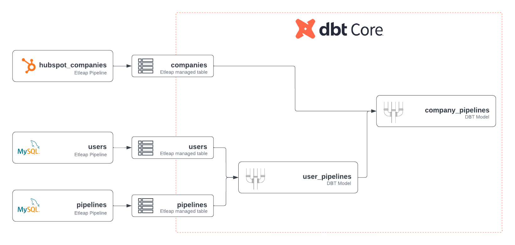
This solution uses Amazon AppFlow to retrieve data from the Jira Cloud. The data is synchronized to an Amazon Simple Storage Service (Amazon S3) bucket using an initial full download and subsequent incremental downloads of changes. When new data arrives in the S3 bucket, an AWS Step Functions workflow is triggered that orchestrates extract, transform, and load (ETL) activities using AWS Glue crawlers and AWS Glue DataBrew. The data is then available in the AWS Glue Data Catalog and can be queried by services such as Amazon Athena, Amazon QuickSight, and Amazon Redshift Spectrum. The solution is completely automated and serverless, resulting in low operational overhead. When this setup is complete, your Jira data will be automatically ingested and kept up to date in your data lake!

The following diagram illustrates the solution architecture.

The Jira Appflow Architecture is shown. The Jira Cloud data is retrieved by Amazon AppFlow and is stored in Amazon S3. This triggers an Amazon EventBridge event that runs an AWS Step Functions workflow. The workflow uses AWS Glue to catalog and transform the data, The data is then queried with QuickSight.

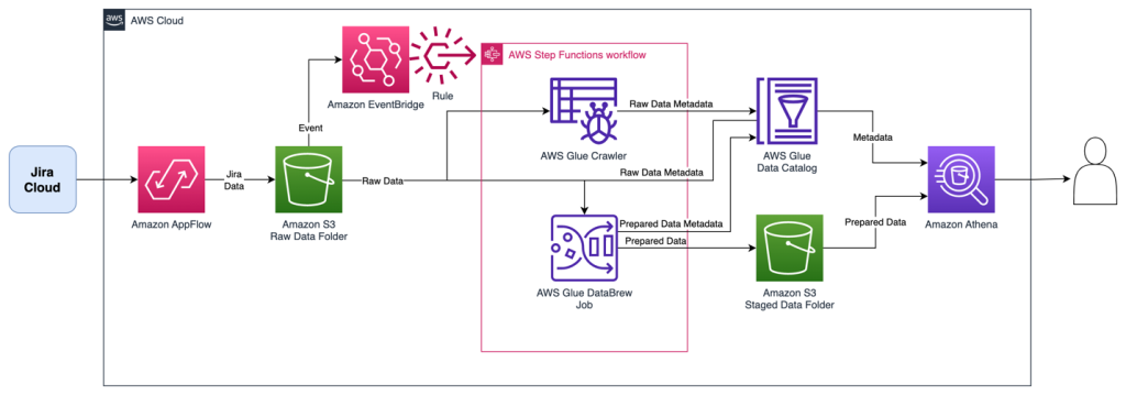
The Step Functions workflow orchestrates the following ETL activities, resulting in two tables:

  • An AWS Glue crawler collects all downloads into a single AWS Glue table named jira_raw. This table is comprised of a mix of full and incremental downloads from Jira, with many versions of the same records representing changes over time.
  • A DataBrew job prepares the data for reporting by unpacking key-value pairs in the fields, as well as removing depreciated records as they are updated in subsequent change data captures. This reporting-ready data will available in an AWS Glue table named jira_data.

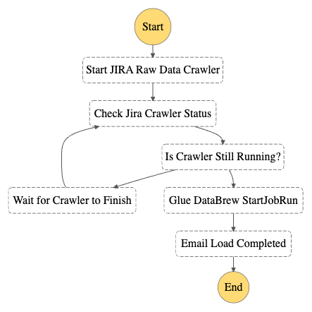
The following figure shows the Step Functions workflow.

A diagram represents the AWS Step Functions workflow. It contains the steps to run an AWS Crawler, wait for it's completion, and then run a AWS Glue DataBrew data transformation job.

Prerequisites

This solution requires the following:

  • Administrative access to your Jira Cloud instance, and an associated Jira Cloud developer account.
  • An AWS account and a login with access to the AWS Management Console. Your login will need AWS Identity and Access Management (IAM) permissions to create and access the resources in your AWS account.
  • Basic knowledge of AWS and working knowledge of Jira administration.

Configure the Jira Instance

After logging in to your Jira Cloud instance, you establish a Jira project with associated epics and issues to download into a data lake. If you’re starting with a new Jira instance, it helps to have at least one project with a sampling of epics and issues for the initial data download, because it allows you to create an initial dataset without errors or missing fields. Note that you may have multiple projects as well.

An image show a Jira Cloud example, with several issues arranged in a Kansan board.

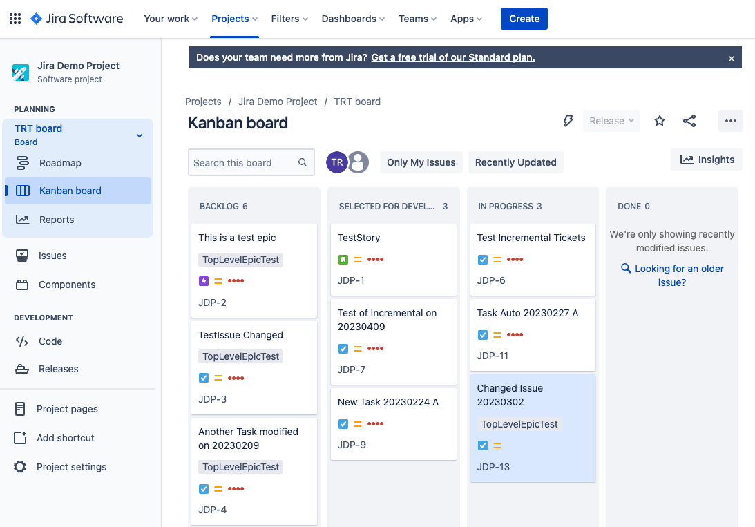
After you have established your Jira project and populated it with epics and issues, ensure you also have access to the Jira developer portal. In later steps, you use this developer portal to establish authentication and permissions for the Amazon AppFlow connection.

Provision resources with AWS CloudFormation

For the initial setup, you launch an AWS CloudFormation stack to create an S3 bucket to store data, IAM roles for data access, and the AWS Glue crawler and Data Catalog components. Complete the following steps:

  1. Sign in to your AWS account.
  2. Click Launch Stack:
  3. For Stack name, enter a name for the stack (the default is aws-blog-jira-datalake-with-AppFlow).
  4. For GlueDatabaseName, enter a unique name for the Data Catalog database to hold the Jira data table metadata (the default is jiralake).
  5. For InitialRunFlag, choose Setup. This mode will scan all data and disable the change data capture (CDC) features of the stack. (Because this is the initial load, the stack needs an initial data load before you configure CDC in later steps.)
  6. Under Capabilities and transforms, select the acknowledgement check boxes to allow IAM resources to be created within your AWS account.
  7. Review the parameters and choose Create stack to deploy the CloudFormation stack. This process will take around 5–10 minutes to complete.
    An image depicts the Amazon CloudFormation configuration steps, including setting a stack name, setting parameters to "jiralake" and "Setup" mode, and checking all IAM capabilities requested.
  8. After the stack is deployed, review the Outputs tab for the stack and collect the following values to use when you set up Amazon AppFlow:
    • Amazon AppFlow destination bucket (o01AppFlowBucket)
    • Amazon AppFlow destination bucket path (o02AppFlowPath)
    • Role for Amazon AppFlow Jira connector (o03AppFlowRole)
      An image demonstrating the Amazon Cloudformation "Outputs" tab, highlighting the values to add to the Amazon AppFlow configuration.

Configure Jira Cloud

Next, you configure your Jira Cloud instance for access by Amazon AppFlow. For full instructions, refer to Jira Cloud connector for Amazon AppFlow. The following steps summarize these instructions and discuss the specific configuration to enable OAuth in the Jira Cloud:

  1. Open the Jira developer portal.
  2. Create the OAuth 2 integration from the developer application console by choosing Create an OAuth 2.0 Integration. This will provide a login mechanism for AppFlow.
  3. Enable fine-grained permissions. See Recommended scopes for the permission settings to grant AppFlow appropriate access to your Jira instance.
  4. Add the following permission scopes to your OAuth app:
    1. manage:jira-configuration
    2. read:field-configuration:jira
  5. Under Authorization, set the Call Back URL to return to Amazon AppFlow with the URL https://us-east-1.console.aws.amazon.com/AppFlow/oauth.
  6. Under Settings, note the client ID and secret to use in later steps to set up authentication from Amazon AppFlow.

Create the Amazon AppFlow Jira Cloud connection

In this step, you configure Amazon AppFlow to run a one-time full data fetch of all your data, establishing the initial data lake:

  1. On the Amazon AppFlow console, choose Connectors in the navigation pane.
  2. Search for the Jira Cloud connector.
  3. Choose Create flow on the connector tile to create the connection to your Jira instance.
    An image of Amazon AppFlor, showing the search for the "Jira Cloud" connector.
  4. For Flow name, enter a name for the flow (for example, JiraLakeFlow).
  5. Leave the Data encryption setting as the default.
  6. Choose Next.
    The Amazon AppFlow Jira connector configuration, showing the Flow name set to "JiraLakeFlow" and clicking the "next" button.
  7. For Source name, keep the default of Jira Cloud.
  8. Choose Create new connection under Jira Cloud connection.
  9. In the Connect to Jira Cloud section, enter the values for Client ID, Client secret, and Jira Cloud Site that you collected earlier. This provides the authentication from AppFlow to Jira Cloud.
  10. For Connection Name, enter a connection name (for example, JiraLakeCloudConnection).
  11. Choose Connect. You will be prompted to allow your OAuth app to access your Atlassian account to verify authentication.
    An image of the Amazon AppFlow conflagration, reflecting the completion of the prior steps.
  12. In the Authorize App window that pops up, choose Accept.
  13. With the connection created, return to the Configure flow section on the Amazon AppFlow console.
  14. For API version, choose V2 to use the latest Jira query API.
  15. For Jira Cloud object, choose Issue to query and download all issues and associated details.
    An image of the Amazon AppFlow configuration, reflecting the completion of the prior steps.
  16. For Destination Name in the Destination Details section, choose Amazon S3.
  17. For Bucket details, choose the S3 bucket name that matches the Amazon AppFlow destination bucket value that you collected from the outputs of the CloudFormation stack.
  18. Enter the Amazon AppFlow destination bucket path to complete the full S3 path. This will send the Jira data to the S3 bucket created by the CloudFormation script.
  19. Leave Catalog your data in the AWS Glue Data Catalog unselected. The CloudFormation script uses an AWS Glue crawler to update the Data Catalog in a different manner, grouping all the downloads into a common table, so we disable the update here.
  20. For File format settings, select Parquet format and select Preserve source data types in Parquet output. Parquet is a columnar format to optimize subsequent querying.
  21. Select Add a timestamp to the file name for Filename preference. This will allow you to easily find data files downloaded at a specific date and time.
    An image of the Amazon AppFlow configuration, reflecting the completion of the prior steps.
  22. For now, select Run on Demand for the Flow trigger to run the full load flow manually. You will schedule downloads in a later step when implementing CDC.
  23. Choose Next.
    An image of the Amazon AppFlow Flow Trigger configuration, reflecting the completion of the prior steps.
  24. On the Map data fields page, select Manually map fields.
  25. For Source to destination field mapping, choose the drop-down box under Source field name and select Map all fields directly. This will bring down all fields as they are received, because we will instead implement data preparation in later steps.
    An image of the Amazon AppFlow configuration, reflecting the completion of steps 24 & 25.
  26. Under Partition and aggregation settings, you can set up the partitions in a way that works for your use case. For this example, we use a daily partition, so select Date and time and choose Daily.
  27. For Aggregation settings, leave it as the default of Don’t aggregate.
  28. Choose Next.
    An image of the Amazon AppFlow configuration, reflecting the completion of steps 26-28.
  29. On the Add filters page, you can create filters to only download specific data. For this example, you download all the data, so choose Next.
  30. Review and choose Create flow.
  31. When the flow is created, choose Run flow to start the initial data seeding. After some time, you should receive a banner indicating the run finished successfully.
    An image of the Amazon AppFlow configuration, reflecting the completion of step 31.

Review seed data

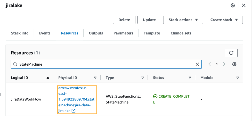
At this stage in the process, you now have data in your S3 environment. When new data files are created in the S3 bucket, it will automatically run an AWS Glue crawler to catalog the new data. You can see if it’s complete by reviewing the Step Functions state machine for a Succeeded run status. There is a link to the state machine on the CloudFormation stack’s Resources tab, which will redirect you to the Step Functions state machine.

A image showing the CloudFormation resources tab of the stack, with a link to the AWS Step Functions workflow.

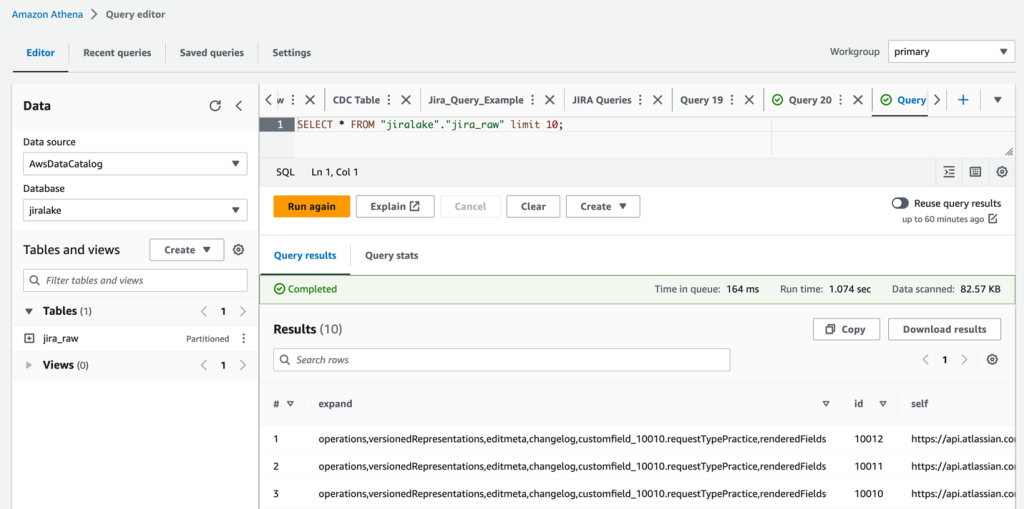
When the state machine is complete, it’s time to review the raw Jira data with Athena. The database is as you specified in the CloudFormation stack (jiralake by default), and the table name is jira_raw. If you kept the default AWS Glue database name of jiralake, the Athena SQL is as follows:

SELECT * FROM "jiralake"."jira_raw" limit 10;

If you explore the data, you’ll notice that most of the data you would want to work with is actually packed into a column called fields. This means the data is not available as columns in your Athena queries, making it harder to select, filter, and sort individual fields within an Athena SQL query. This will be addressed in the next steps.

An image demonstrating the Amazon Athena query SELECT * FROM "jiralake"."jira_raw" limit 10;

Set up CDC and unpack the fields columns

To add the ongoing CDC and reformat the data for analytics, we introduce a DataBrew job to transform the data and filter to the most recent version of each record as changes come in. You can do this by updating the CloudFormation stack with a flag that includes the CDC and data transformation steps.

  1. On the AWS CloudFormation console, return to the stack.
  2. Choose Update.
  3. Select Use current template and choose Next.
    An image showing Amazon CloudFormation, with steps 1-3 complete.
  4. For SetupOrCDC, choose CDC, then choose Next. This will enable both the CDC steps and the data transformation steps for the Jira data.
    An image showing Amazon CloudFormation, with step 4 complete.
  5. Continue choosing Next until you reach the Review section.
  6. Select I acknowledge that AWS CloudFormation might create IAM resources, then choose Submit.
    An image showing Amazon CloudFormation, with step 5-6 complete.
  7. Return to the Amazon AppFlow console and open your flow.
  8. On the Actions menu, choose Edit flow. We will now edit the flow trigger to run an incremental load on a periodic basis.
  9. Select Run flow on schedule.
  10. Configure the desired repeats, as well as start time and date. For this example, we choose Daily for Repeats and enter 1 for the number of days you’ll have the flow trigger. For Starting at, enter 01:00.
  11. Select Incremental transfer for Transfer mode.
  12. Choose Updated on the drop-down menu so that changes will be captured based on when the records were updated.
  13. Choose Save. With these settings in our example, the run will happen nightly at 1:00 AM.
    An image showing the Flow Trigger, with incremental transfer selected.

Review the analytics data

When the next incremental load occurs that results in new data, the Step Functions workflow will start the DataBrew job and populate a new staged analytical data table named jira_data in your Data Catalog database. If you don’t want to wait, you can trigger the Step Functions workflow manually.

The DataBrew job performs data transformation and filtering tasks. The job unpacks the key-values from the Jira JSON data and the raw Jira data, resulting in a tabular data schema that facilitates use with BI and AI/ML tools. As Jira items are changed, the changed item’s data is resent, resulting in multiple versions of an item in the raw data feed. The DataBrew job filters the raw data feed so that the resulting data table only contains the most recent version of each item. You could enhance this DataBrew job to further customize the data for your needs, such as renaming the generic Jira custom field names to reflect their business meaning.

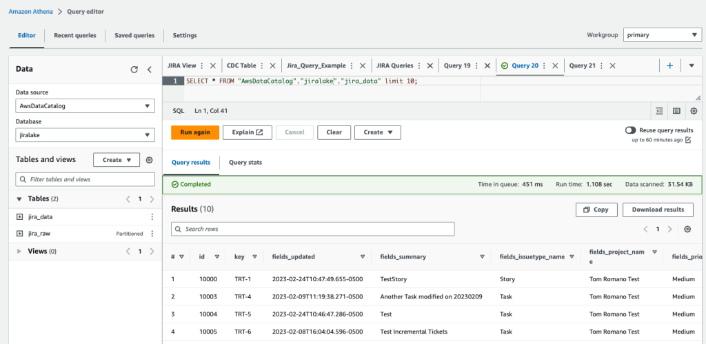
When the Step Functions workflow is complete, we can query the data in Athena again using the following query:

SELECT * FROM "jiralake"."jira_data" limit 10;

You can see that in our transformed jira_data table, the nested JSON fields are broken out into their own columns for each field. You will also notice that we’ve filtered out obsolete records that have been superseded by more recent record updates in later data loads so the data is fresh. If you want to rename custom fields, remove columns, or restructure what comes out of the nested JSON, you can modify the DataBrew recipe to accomplish this. At this point, the data is ready to be used by your analytics tools, such as Amazon QuickSight.

An image demonstrating the Amazon Athena query SELECT * FROM "jiralake"."jira_data" limit 10;

Clean up

If you would like to discontinue this solution, you can remove it with the following steps:

  1. On the Amazon AppFlow console, deactivate the flow for Jira, and optionally delete it.
  2. On the Amazon S3 console, select the S3 bucket for the stack, and empty the bucket to delete the existing data.
  3. On the AWS CloudFormation console, delete the CloudFormation stack that you deployed.

Conclusion

In this post, we created a serverless incremental data load process for Jira that will synchronize data while handling custom fields using Amazon AppFlow, AWS Glue, and Step Functions. The approach uses Amazon AppFlow to incrementally load the data into Amazon S3. We then use AWS Glue and Step Functions to manage the extraction of the Jira custom fields and load them in a format to be queried by analytics services such as Athena, QuickSight, or Redshift Spectrum, or AI/ML services like Amazon SageMaker.

To learn more about AWS Glue and DataBrew, refer to Getting started with AWS Glue DataBrew. With DataBrew, you can take the sample data transformation in this project and customize the output to meet your specific needs. This could include renaming columns, creating additional fields, and more.

To learn more about Amazon AppFlow, refer to Getting started with Amazon AppFlow. Note that Amazon AppFlow supports integrations with many SaaS applications in addition to the Jira Cloud.

To learn more about orchestrating flows with Step Functions, see Create a Serverless Workflow with AWS Step Functions and AWS Lambda. The workflow could be enhanced to load the data into a data warehouse, such as Amazon Redshift, or trigger a refresh of a QuickSight dataset for analytics and reporting.

In future posts, we will cover how to unnest parent-child relationships within the Jira data using Athena and how to visualize the data using QuickSight.


About the Authors

Tom Romano is a Sr. Solutions Architect for AWS World Wide Public Sector from Tampa, FL, and assists GovTech and EdTech customers as they create new solutions that are cloud native, event driven, and serverless. He is an enthusiastic Python programmer for both application development and data analytics, and is an Analytics Specialist. In his free time, Tom flies remote control model airplanes and enjoys vacationing with his family around Florida and the Caribbean.

Shane Thompson is a Sr. Solutions Architect based out of San Luis Obispo, California, working with AWS Startups. He works with customers who use AI/ML in their business model and is passionate about democratizing AI/ML so that all customers can benefit from it. In his free time, Shane loves to spend time with his family and travel around the world.

A side-by-side comparison of Apache Spark and Apache Flink for common streaming use cases

Post Syndicated from Deepthi Mohan original https://aws.amazon.com/blogs/big-data/a-side-by-side-comparison-of-apache-spark-and-apache-flink-for-common-streaming-use-cases/

Apache Flink and Apache Spark are both open-source, distributed data processing frameworks used widely for big data processing and analytics. Spark is known for its ease of use, high-level APIs, and the ability to process large amounts of data. Flink shines in its ability to handle processing of data streams in real-time and low-latency stateful computations. Both support a variety of programming languages, scalable solutions for handling large amounts of data, and a wide range of connectors. Historically, Spark started out as a batch-first framework and Flink began as a streaming-first framework.

In this post, we share a comparative study of streaming patterns that are commonly used to build stream processing applications, how they can be solved using Spark (primarily Spark Structured Streaming) and Flink, and the minor variations in their approach. Examples cover code snippets in Python and SQL for both frameworks across three major themes: data preparation, data processing, and data enrichment. If you are a Spark user looking to solve your stream processing use cases using Flink, this post is for you. We do not intend to cover the choice of technology between Spark and Flink because it’s important to evaluate both frameworks for your specific workload and how the choice fits in your architecture; rather, this post highlights key differences for use cases that both these technologies are commonly considered for.

Apache Flink offers layered APIs that offer different levels of expressiveness and control and are designed to target different types of use cases. The three layers of API are Process Functions (also known as the Stateful Stream Processing API), DataStream, and Table and SQL. The Stateful Stream Processing API requires writing verbose code but offers the most control over time and state, which are core concepts in stateful stream processing. The DataStream API supports Java, Scala, and Python and offers primitives for many common stream processing operations, as well as a balance between code verbosity or expressiveness and control. The Table and SQL APIs are relational APIs that offer support for Java, Scala, Python, and SQL. They offer the highest abstraction and intuitive, SQL-like declarative control over data streams. Flink also allows seamless transition and switching across these APIs. To learn more about Flink’s layered APIs, refer to layered APIs.

Apache Spark Structured Streaming offers the Dataset and DataFrames APIs, which provide high-level declarative streaming APIs to represent static, bounded data as well as streaming, unbounded data. Operations are supported in Scala, Java, Python, and R. Spark has a rich function set and syntax with simple constructs for selection, aggregation, windowing, joins, and more. You can also use the Streaming Table API to read tables as streaming DataFrames as an extension to the DataFrames API. Although it’s hard to draw direct parallels between Flink and Spark across all stream processing constructs, at a very high level, we could say Spark Structured Streaming APIs are equivalent to Flink’s Table and SQL APIs. Spark Structured Streaming, however, does not yet (at the time of this writing) offer an equivalent to the lower-level APIs in Flink that offer granular control of time and state.

Both Flink and Spark Structured Streaming (referenced as Spark henceforth) are evolving projects. The following table provides a simple comparison of Flink and Spark capabilities for common streaming primitives (as of this writing).

. Flink Spark
Row-based processing Yes Yes
User-defined functions Yes Yes
Fine-grained access to state Yes, via DataStream and low-level APIs No
Control when state eviction occurs Yes, via DataStream and low-level APIs No
Flexible data structures for state storage and querying Yes, via DataStream and low-level APIs No
Timers for processing and stateful operations Yes, via low level APIs No

In the following sections, we cover the greatest common factors so that we can showcase how Spark users can relate to Flink and vice versa. To learn more about Flink’s low-level APIs, refer to Process Function. For the sake of simplicity, we cover the four use cases in this post using the Flink Table API. We use a combination of Python and SQL for an apples-to-apples comparison with Spark.

Data preparation

In this section, we compare data preparation methods for Spark and Flink.

Reading data

We first look at the simplest ways to read data from a data stream. The following sections assume the following schema for messages:

symbol: string,
price: int,
timestamp: timestamp,
company_info:
{
    name: string,
    employees_count: int
}

Reading data from a source in Spark Structured Streaming

In Spark Structured Streaming, we use a streaming DataFrame in Python that directly reads the data in JSON format:

spark = ...  # spark session

# specify schema
stock_ticker_schema = ...

# Create a streaming DataFrame
df = spark.readStream \
    .format("kafka") \
    .option("kafka.bootstrap.servers", "mybroker1:port") \
    .option("topic", "stock_ticker") \
    .load()
    .select(from_json(col("value"), stock_ticker_schema).alias("ticker_data")) \
    .select(col("ticker_data.*"))

Note that we have to supply a schema object that captures our stock ticker schema (stock_ticker_schema). Compare this to the approach for Flink in the next section.

Reading data from a source using Flink Table API

For Flink, we use the SQL DDL statement CREATE TABLE. You can specify the schema of the stream just like you would any SQL table. The WITH clause allows us to specify the connector to the data stream (Kafka in this case), the associated properties for the connector, and data format specifications. See the following code:

# Create table using DDL

CREATE TABLE stock_ticker (
  symbol string,
  price INT,
  timestamp TIMESTAMP(3),
  company_info STRING,
  WATERMARK FOR timestamp AS timestamp - INTERVAL '3' MINUTE
) WITH (
 'connector' = 'kafka',
 'topic' = 'stock_ticker',
 'properties.bootstrap.servers' = 'mybroker1:port',
 'properties.group.id' = 'testGroup',
 'format' = 'json',
 'json.fail-on-missing-field' = 'false',
 'json.ignore-parse-errors' = 'true'
)

JSON flattening

JSON flattening is the process of converting a nested or hierarchical JSON object into a flat, single-level structure. This converts multiple levels of nesting into an object where all the keys and values are at the same level. Keys are combined using a delimiter such as a period (.) or underscore (_) to denote the original hierarchy. JSON flattening is useful when you need to work with a more simplified format. In both Spark and Flink, nested JSONs can be complicated to work with and may need additional processing or user-defined functions to manipulate. Flattened JSONs can simplify processing and improve performance due to reduced computational overhead, especially with operations like complex joins, aggregations, and windowing. In addition, flattened JSONs can help in easier debugging and troubleshooting data processing pipelines because there are fewer levels of nesting to navigate.

JSON flattening in Spark Structured Streaming

JSON flattening in Spark Structured Streaming requires you to use the select method and specify the schema that you need flattened. JSON flattening in Spark Structured Streaming involves specifying the nested field name that you’d like surfaced to the top-level list of fields. In the following example, company_info is a nested field and within company_info, there’s a field called company_name. With the following query, we’re flattening company_info.name to company_name:

stock_ticker_df = ...  # Streaming DataFrame w/ schema shown above

stock_ticker_df.select("symbol", "timestamp", "price", "company_info.name" as "company_name")

JSON flattening in Flink

In Flink SQL, you can use the JSON_VALUE function. Note that you can use this function only in Flink versions equal to or greater than 1.14. See the following code:

SELECT
   symbol,
   timestamp,
   price,
   JSON_VALUE(company_info, 'lax $.name' DEFAULT NULL ON EMPTY) AS company_name
FROM
   stock_ticker

The term lax in the preceding query has to do with JSON path expression handling in Flink SQL. For more information, refer to System (Built-in) Functions.

Data processing

Now that you have read the data, we can look at a few common data processing patterns.

Deduplication

Data deduplication in stream processing is crucial for maintaining data quality and ensuring consistency. It enhances efficiency by reducing the strain on the processing from duplicate data and helps with cost savings on storage and processing.

Spark Streaming deduplication query

The following code snippet is related to a Spark Streaming DataFrame named stock_ticker. The code performs an operation to drop duplicate rows based on the symbol column. The dropDuplicates method is used to eliminate duplicate rows in a DataFrame based on one or more columns.

stock_ticker = ...  # Streaming DataFrame w/ schema shown above

stock_ticker.dropDuplicates("symbol")

Flink deduplication query

The following code shows the Flink SQL equivalent to deduplicate data based on the symbol column. The query retrieves the first row for each distinct value in the symbol column from the stock_ticker stream, based on the ascending order of proctime:

SELECT symbol, timestamp, price
FROM (
  SELECT *,
    ROW_NUMBER() OVER (PARTITION BY symbol ORDER BY proctime ASC) AS row_num
  FROM stock_ticker)
WHERE row_num = 1

Windowing

Windowing in streaming data is a fundamental construct to process data within specifications. Windows commonly have time bounds, number of records, or other criteria. These time bounds bucketize continuous unbounded data streams into manageable chunks called windows for processing. Windows help in analyzing data and gaining insights in real time while maintaining processing efficiency. Analyses or operations are performed on constantly updating streaming data within a window.

There are two common time-based windows used both in Spark Streaming and Flink that we will detail in this post: tumbling and sliding windows. A tumbling window is a time-based window that is a fixed size and doesn’t have any overlapping intervals. A sliding window is a time-based window that is a fixed size and moves forward in fixed intervals that can be overlapping.

Spark Streaming tumbling window query

The following is a Spark Streaming tumbling window query with a window size of 10 minutes:

stock_ticker = ...  # Streaming DataFrame w/ schema shown above

# Get max stock price in tumbling window
# of size 10 minutes
visitsByWindowAndUser = visits
   .withWatermark("timestamp", "3 minutes")
   .groupBy(
      window(stock_ticker.timestamp, "10 minutes"),
      stock_ticker.symbol)
   .max(stock_ticker.price)

Flink Streaming tumbling window query

The following is an equivalent tumbling window query in Flink with a window size of 10 minutes:

SELECT symbol, MAX(price)
  FROM TABLE(
    TUMBLE(TABLE stock_ticker, DESCRIPTOR(timestamp), INTERVAL '10' MINUTES))
  GROUP BY ticker;

Spark Streaming sliding window query

The following is a Spark Streaming sliding window query with a window size of 10 minutes and slide interval of 5 minutes:

stock_ticker = ...  # Streaming DataFrame w/ schema shown above

# Get max stock price in sliding window
# of size 10 minutes and slide interval of size
# 5 minutes

visitsByWindowAndUser = visits
   .withWatermark("timestamp", "3 minutes")
   .groupBy(
      window(stock_ticker.timestamp, "10 minutes", "5 minutes"),
      stock_ticker.symbol)
   .max(stock_ticker.price)

Flink Streaming sliding window query

The following is a Flink sliding window query with a window size of 10 minutes and slide interval of 5 minutes:

SELECT symbol, MAX(price)
  FROM TABLE(
    HOP(TABLE stock_ticker, DESCRIPTOR(timestamp), INTERVAL '5' MINUTES, INTERVAL '10' MINUTES))
  GROUP BY ticker;

Handling late data

Both Spark Structured Streaming and Flink support event time processing, where a field within the payload can be used for defining time windows as distinct from the wall clock time of the machines doing the processing. Both Flink and Spark use watermarking for this purpose.

Watermarking is used in stream processing engines to handle delays. A watermark is like a timer that sets how long the system can wait for late events. If an event arrives and is within the set time (watermark), the system will use it to update a request. If it’s later than the watermark, the system will ignore it.

In the preceding windowing queries, you specify the lateness threshold in Spark using the following code:

.withWatermark("timestamp", "3 minutes")

This means that any records that are 3 minutes late as tracked by the event time clock will be discarded.

In contrast, with the Flink Table API, you can specify an analogous lateness threshold directly in the DDL:

WATERMARK FOR timestamp AS timestamp - INTERVAL '3' MINUTE

Note that Flink provides additional constructs for specifying lateness across its various APIs.

Data enrichment

In this section, we compare data enrichment methods with Spark and Flink.

Calling an external API

Calling external APIs from user-defined functions (UDFs) is similar in Spark and Flink. Note that your UDF will be called for every record processed, which can result in the API getting called at a very high request rate. In addition, in production scenarios, your UDF code often gets run in parallel across multiple nodes, further amplifying the request rate.

For the following code snippets, let’s assume that the external API call entails calling the function:

response = my_external_api(request)

External API call in Spark UDF

The following code uses Spark:

class Predict(ScalarFunction):
def open(self, function_context):

with open("resources.zip/resources/model.pkl", "rb") as f:
self.model = pickle.load(f)

def eval(self, x):
return self.model.predict(x)

External API call in Flink UDF

For Flink, assume we define the UDF callExternalAPIUDF, which takes as input the ticker symbol symbol and returns enriched information about the symbol via a REST endpoint. We can then register and call the UDF as follows:

callExternalAPIUDF = udf(callExternalAPIUDF(), result_type=DataTypes.STRING())

SELECT
    symbol, 
    callExternalAPIUDF(symbol) as enriched_symbol
FROM stock_ticker;

Flink UDFs provide an initialization method that gets run one time (as opposed to one time per record processed).

Note that you should use UDFs judiciously as an improperly implemented UDF can cause your job to slow down, cause backpressure, and eventually stall your stream processing application. It’s advisable to use UDFs asynchronously to maintain high throughput, especially for I/O-bound use cases or when dealing with external resources like databases or REST APIs. To learn more about how you can use asynchronous I/O with Apache Flink, refer to Enrich your data stream asynchronously using Amazon Kinesis Data Analytics for Apache Flink.

Conclusion

Apache Flink and Apache Spark are both rapidly evolving projects and provide a fast and efficient way to process big data. This post focused on the top use cases we commonly encountered when customers wanted to see parallels between the two technologies for building real-time stream processing applications. We’ve included samples that were most frequently requested at the time of this writing. Let us know if you’d like more examples in the comments section.


About the author

Deepthi Mohan is a Principal Product Manager on the Amazon Kinesis Data Analytics team.

Karthi Thyagarajan was a Principal Solutions Architect on the Amazon Kinesis team.

Simplify external object access in Amazon Redshift using automatic mounting of the AWS Glue Data Catalog

Post Syndicated from Maneesh Sharma original https://aws.amazon.com/blogs/big-data/simplify-external-object-access-in-amazon-redshift-using-automatic-mounting-of-the-aws-glue-data-catalog/

Amazon Redshift is a petabyte-scale, enterprise-grade cloud data warehouse service delivering the best price-performance. Today, tens of thousands of customers run business-critical workloads on Amazon Redshift to cost-effectively and quickly analyze their data using standard SQL and existing business intelligence (BI) tools.

Amazon Redshift now makes it easier for you to run queries in AWS data lakes by automatically mounting the AWS Glue Data Catalog. You no longer have to create an external schema in Amazon Redshift to use the data lake tables cataloged in the Data Catalog. Now, you can use your AWS Identity and Access Management (IAM) credentials or IAM role to browse the Glue Data Catalog and query data lake tables directly from Amazon Redshift Query Editor v2 or your preferred SQL editors.

This feature is now available in all AWS commercial and US Gov Cloud Regions where Amazon Redshift RA3, Amazon Redshift Serverless, and AWS Glue are available. To learn more about auto-mounting of the Data Catalog in Amazon Redshift, refer to Querying the AWS Glue Data Catalog.

Enabling easy analytics for everyone

Amazon Redshift is helping tens of thousands of customers manage analytics at scale. Amazon Redshift offers a powerful analytics solution that provides access to insights for users of all skill levels. You can take advantage of the following benefits:

  • It enables organizations to analyze diverse data sources, including structured, semi-structured, and unstructured data, facilitating comprehensive data exploration
  • With its high-performance processing capabilities, Amazon Redshift handles large and complex datasets, ensuring fast query response times and supporting real-time analytics
  • Amazon Redshift provides features like Multi-AZ (preview) and cross-Region snapshot copy for high availability and disaster recovery, and provides authentication and authorization mechanisms to make it reliable and secure
  • With features like Amazon Redshift ML, it democratizes ML capabilities across a variety of user personas
  • The flexibility to utilize different table formats such as Apache Hudi, Delta Lake, and Apache Iceberg (preview) optimizes query performance and storage efficiency
  • Integration with advanced analytical tools empowers you to apply sophisticated techniques and build predictive models
  • Scalability and elasticity allow for seamless expansion as data and workloads grow

Overall, Amazon Redshift empowers organizations to uncover valuable insights, enhance decision-making, and gain a competitive edge in today’s data-driven landscape.

Amazon Redshift Top Benefits

Amazon Redshift Top Benefits

The new automatic mounting of the AWS Glue Data Catalog feature enables you to directly query AWS Glue objects in Amazon Redshift without the need to create an external schema for each AWS Glue database you want to query. With automatic mounting the Data Catalog, Amazon Redshift automatically mounts the cluster account’s default Data Catalog during boot or user opt-in as an external database, named awsdatacatalog.

Relevant use cases for automatic mounting of the AWS Glue Data Catalog feature

You can use tools like Amazon EMR to create new data lake schemas in various formats, such as Apache Hudi, Delta Lake, and Apache Iceberg (preview). However, when analysts want to run queries against these schemas, it requires administrators to create external schemas for each AWS Glue database in Amazon Redshift. You can now simplify this integration using automatic mounting of the AWS Glue Data Catalog.

The following diagram illustrates this architecture.

Solution overview

You can now use SQL clients like Amazon Redshift Query Editor v2 to browse and query awsdatacatalog. In Query Editor V2, to connect to the awsdatacatalog database, choose the following:

Complete the following high-level steps to integrate the automatic mounting of the Data Catalog using Query Editor V2 and a third-party SQL client:

  1. Provision resources with AWS CloudFormation to populate Data Catalog objects.
  2. Connect Redshift Serverless and query the Data Catalog as a federated user using Query Editor V2.
  3. Connect with Redshift provisioned cluster and query the Data Catalog using Query Editor V2.
  4. Configure permissions on catalog resources using AWS Lake Formation.
  5. Federate with Redshift Serverless and query the Data Catalog using Query Editor V2 and a third-party SQL client.
  6. Discover the auto-mounted objects.
  7. Connect with Redshift provisioned cluster and query the Data Catalog as a federated user using a third-party client.
  8. Connect with Amazon Redshift and query the Data Catalog as an IAM user using third-party clients.

The following diagram illustrates the solution workflow.

Prerequisites

You should have the following prerequisites:

Provision resources with AWS CloudFormation to populate Data Catalog objects

In this post, we use an AWS Glue crawler to create the external table ny_pub stored in Apache Parquet format in the Amazon Simple Storage Service (Amazon S3) location s3://redshift-demos/data/NY-Pub/. In this step, we create the solution resources using AWS CloudFormation to create a stack named CrawlS3Source-NYTaxiData in either us-east-1 (use the yml download or launch stack) or us-west-2 (use the yml download or launch stack). Stack creation performs the following actions:

  • Creates the crawler NYTaxiCrawler along with the new IAM role AWSGlueServiceRole-RedshiftAutoMount
  • Creates automountdb as the AWS Glue database

When the stack is complete, perform the following steps:

  1. On the AWS Glue console, under Data Catalog in the navigation pane, choose Crawlers.
  2. Open NYTaxiCrawler and choose Run crawler.

After the crawler is complete, you can see a new table called ny_pub in the Data Catalog under the automountdb database.


Alternatively, you can follow the manual instructions from the Amazon Redshift labs to create the ny_pub table.

Connect with Redshift Serverless and query the Data Catalog as a federated user using Query Editor V2

In this section, we use an IAM role with principal tags to enable fine-grained federated authentication to Redshift Serverless to access auto-mounting AWS Glue objects.

Complete the following steps:

  1. Create an IAM role and add following permissions. For this post, we add full AWS Glue, Amazon Redshift, and Amazon S3 permissions for demo purposes. In an actual production scenario, it’s recommended to apply more granular permissions.

  2. On the Tags tab, create a tag with Key as RedshiftDbRoles and Value as automount.
  3. In Query Editor V2, run the following SQL statement as an admin user to create a database role named automount:
    Create role automount;

  4. Grant usage privileges to the database role:
    GRANT USAGE ON DATABASE awsdatacatalog to role automount;

  5. Switch the role to automountrole by passing the account number and role name.
  6. In the Query Editor v2, choose your Redshift Serverless endpoint (right-click) and choose Create connection.
  7. For Authentication, select Federated user.
  8. For Database, enter the database name you want to connect to.
  9. Choose Create connection.

You’re now ready to explore and query the automatic mounting of the Data Catalog in Redshift Serverless.

Connect with Redshift provisioned cluster and query the Data Catalog using Query Editor V2

To connect with Redshift provisioned cluster and access the Data Catalog, make sure you have completed the steps in the preceding section. Then complete the following steps:

  1. Connect to Redshift Query Editor V2 using the database user name and password authentication method. For example, connect to the dev database using the admin user and password.
  2. In an editor tab, assuming the user is present in Amazon Redshift, run the following SQL statement to grant an IAM user access to the Data Catalog:
    GRANT USAGE ON DATABASE awsdatacatalog to "IAMR:automountrole";

  3. As an admin user, choose the Settings icon, choose Account settings, and select Authenticate with IAM credentials.
  4. Choose Save.
  5. Switch roles to automountrole by passing the account number and role name.
  6. Create or edit the connection and use the authentication method Temporary credentials using your IAM identity.

For more information about this authentication method, see Connecting to an Amazon Redshift database.

You are ready to explore and query the automatic mounting of the Data Catalog in Amazon Redshift.

Discover the auto-mounted objects

This section illustrates the SHOW commands for discovery of auto-mounted objects. See the following code:

// Discovery of Glue databases at the schema level 
SHOW SCHEMAS FROM DATABASE awsdatacatalog;

// Discovery of Glue tables 
 Syntax: SHOW TABLES FROM SCHEMA awsdatacatalog.<glue_db_name>;
Example: SHOW TABLES FROM SCHEMA awsdatacatalog.automountdb;

// Disocvery of Glue table columns 
 Syntax: SHOW COLUMNS FROM TABLE awsdatacatalog.<glue_db_name>.<glue_table_name>;
Example: SHOW COLUMNS FROM TABLE awsdatacatalog.automountdb.ny_pub;

Configure permissions on catalog resources using AWS Lake Formation

To maintain backward compatibility with AWS Glue, Lake Formation has the following initial security settings:

  • The Super permission is granted to the group IAMAllowedPrincipals on all existing Data Catalog resources
  • The Use only IAM access control setting is enabled for new Data Catalog resources

These settings effectively cause access to Data Catalog resources and Amazon S3 locations to be controlled solely by IAM policies. Individual Lake Formation permissions are not in effect.

In this step, we will configure permissions on catalog resources using AWS Lake Formation. Before you create the Data Catalog, you need to update the default settings of Lake Formation so that access to Data Catalog resources (databases and tables) is managed by Lake Formation permissions:

  1. Change the default security settings for new resources. For instructions, see Change the default permission model.
  2. Change the settings for existing Data Catalog resources. For instructions, see Upgrading AWS Glue data permissions to the AWS Lake Formation model.

For more information, refer to Changing the default settings for your data lake.

Federate with Redshift Serverless and query the Data Catalog using Query Editor V2 and a third-party SQL client

With Redshift Serverless, you can connect to awsdatacatalog from a third-party client as a federated user from any identity provider (IdP). In this section, we will configure permission on catalog resources for Federated IAM role in AWS Lake Formation. Using AWS Lake Formation with Redshift, currently permission can be applied on IAM user or IAM role level.

To connect as a federated user, we will be using Redshift Serverless. For setup instructions, refer to Single sign-on with Amazon Redshift Serverless with Okta using Amazon Redshift Query Editor v2 and third-party SQL clients.

There are additional changes required on following resources:

  1. In Amazon Redshift, as an admin user, grant the usage to each federated user who needs access on awsdatacatalog:
    GRANT USAGE ON DATABASE awsdatacatalog to "IAMR:[email protected]";

If the user doesn’t exist in Amazon Redshift, you may need to create the IAM user with the password disabled as shown in the following code and then grant usage on awsdatacatalog:

Create User "IAMR:[email protected]" with password disable;
  1. On the Lake Formation console, assign permissions on the AWS Glue database to the IAM role that you created as part of the federated setup.
    1. Under Principals, select IAM users and roles.
    2. Choose IAM role oktarole.
    3. Apply catalog resource permissions, selecting automountdb database and granting appropriate table permissions.
  2. Update the IAM role used in the federation setup. In addition to the permissions added to the IAM role, you need to add AWS Glue permissions and Amazon S3 permissions to access objects from Amazon S3. For this post, we add full AWS Glue and AWS S3 permissions for demo purposes. In an actual production scenario, it’s recommended to apply more granular permissions.

Now you’re ready to connect to Redshift Serverless using the Query Editor V2 and federated login.

  1. Use the SSO URL from Okta and log in to your Okta account with your user credentials. For this demo, we log in with user Ethan.
  2. In the Query Editor v2, choose your Redshift Serverless instance (right-click) and choose Create connection.
  3. For Authentication, select Federated user.
  4. For Database, enter the database name you want to connect to.
  5. Choose Create connection.
  6. Run the command select current_user to validate that you are logged in as a federated user.

User Ethan will be able to explore and access awsdatacatalog data.

To connect Redshift Serverless with a third-party client, make sure you have followed all the previous steps.

For SQLWorkbench setup, refer to the section Configure the SQL client (SQL Workbench/J) in Single sign-on with Amazon Redshift Serverless with Okta using Amazon Redshift Query Editor v2 and third-party SQL clients.

The following screenshot shows that federated user ethan is able to query the awsdatacatalog tables using three-part notation:

Connect with Redshift provisioned cluster and query the Data Catalog as a federated user using third-party clients

With Redshift provisioned cluster, you can connect with awsdatacatalog from a third-party client as a federated user from any IdP.

To connect as a federated user with the Redshift provisioned cluster, you need to follow the steps in the previous section that detailed how to connect with Redshift Serverless and query the Data Catalog as a federated user using Query Editor V2 and a third-party SQL client.

There are additional changes required in IAM policy. Update the IAM policy with the following code to use the GetClusterCredentialsWithIAM API:

{
    "Version": "2012-10-17",
    "Statement": [
        {
            "Sid": "VisualEditor0",
            "Effect": "Allow",
            "Action": "iam:ListGroups",
            "Resource": "*"
        },
        {
            "Sid": "VisualEditor1",
            "Effect": "Allow",
            "Action": "redshift:GetClusterCredentialsWithIAM",
            "Resource": "arn:aws:redshift:us-east-2:01234567891:dbname:redshift-cluster-1/dev"
        }
    ]
}

Now you’re ready to connect to Redshift provisioned cluster using a third-party SQL client as a federated user.

For SQLWorkbench setup, refer to the section Configure the SQL client (SQL Workbench/J) in the post Single sign-on with Amazon Redshift Serverless with Okta using Amazon Redshift Query Editor v2 and third-party SQL clients.

Make the following changes:

  • Use the latest Redshift JDBC driver because it only supports querying the auto-mounted Data Catalog table for federated users
  • For URL, enter jdbc:redshift:iam://<cluster endpoint>:<port>:<databasename>?groupfederation=true. For example, jdbc:redshift:iam://redshift-cluster-1.abdef0abc0ab.us-east-2.redshift.amazonaws.com:5439/dev?groupfederation=true.

In the preceding URL, groupfederation is a mandatory parameter that allows you to authenticate with the IAM credentials.

The following screenshot shows that federated user ethan is able to query the awsdatacatalog tables using three-part notation.

Connect and query the Data Catalog as an IAM user using third-party clients

In this section, we provide instructions to set up a SQL client to query the auto-mounted awsdatacatalog.

Use three-part notation to reference the awsdatacatalog table in your SELECT statement. The first part is the database name, the second part is the AWS Glue database name, and the third part is the AWS Glue table name:

SELECT * FROM awsdatacatalog.<aws-glue-db-name>.<aws-glue-table-name>;

You can perform various scenarios that read the Data Catalog data and populate Redshift tables.

For this post, we use SQLWorkbench/J as the SQL client to query the Data Catalog. To set up SQL Workbench/J, complete the following steps:

  1. Create a new connection in SQL Workbench/J and choose Amazon Redshift as the driver.
  2. Choose Manage drivers and add all the files from the downloaded AWS JDBC driver pack .zip file (remember to unzip the .zip file).

You must use the latest Redshift JDBC driver because it only supports querying the auto-mounted Data Catalog table.

  1. For URL, enter jdbc:redshift:iam://<cluster endpoint>:<port>:<databasename>?profile=<profilename>&groupfederation=true. For example, jdbc:redshift:iam://redshift-cluster-1.abdef0abc0ab.us-east-2.redshift.amazonaws.com:5439/dev?profile=user2&groupfederation=true.

We are using profile-based credentials as an example. You can use any AWS profile or IAM credential-based authentication as per your requirement. For more information on IAM credentials, refer to Options for providing IAM credentials.

The following screenshot shows that IAM user johndoe is able to list the awsdatacatalog tables using the SHOW command.

The following screenshot shows that IAM user johndoe is able to query the awsdatacatalog tables using three-part notation:

If you get the following error while using groupfederation=true, you need to use the latest Redshift driver:

Something unusual has occurred to cause the driver to fail. Please report this exception:Authentication with plugin is not supported for group federation [SQL State=99999]

Clean up

Complete the following steps to clean up your resources:

  1. Delete the IAM role automountrole.
  2. Delete the CloudFormation stack CrawlS3Source-NYTaxiData to clean up the crawler NYTaxiCrawler, the automountdb database from the Data Catalog, and the IAM role AWSGlueServiceRole-RedshiftAutoMount.
  3. Update the default settings of Lake Formation:
    1. In the navigation pane, under Data catalog, choose Settings.
    2. Select both access control options choose Save.
    3. In the navigation pane, under Permissions, choose Administrative roles and tasks.
    4. In the Database creators section, choose Grant.
    5. Search for IAMAllowedPrincipals and select Create database permission.
    6. Choose Grant.

Considerations

Note the following considerations:

  • The Data Catalog auto-mount provides ease of use to analysts or database users. The security setup (setting up the permissions model or data governance) is owned by account and database administrators.
    • To achieve fine-grained access control, build a permissions model in AWS Lake Formation.
    • If the permissions have to be maintained at the Redshift database level, leave the AWS Lake Formation default settings as is and then run grant/revoke in Amazon Redshift.
  • If you are using a third-party SQL editor, and your query tool does not support browsing of multiple databases, you can use the “SHOW“ commands to list your AWS Glue databases and tables. You can also query awsdatacatalog objects using three-part notation (SELECT * FROM awsdatacatalog.<aws-glue-db-name>.<aws-glue-table-name>;) provided you have access to the external objects based on the permission model.

Conclusion

In this post, we introduced the automatic mounting of AWS Glue Data Catalog, which makes it easier for customers to run queries in their data lakes. This feature streamlines data governance and access control, eliminating the need to create an external schema in Amazon Redshift to use the data lake tables cataloged in AWS Glue Data Catalog. We showed how you can manage permission on auto-mounted AWS Glue-based objects using Lake Formation. The permission model can be easily managed and organized by administrators, allowing database users to seamlessly access external objects they have been granted access to.

As we strive for enhanced usability in Amazon Redshift, we prioritize unified data governance and fine-grained access control. This feature minimizes manual effort while ensuring the necessary security measures for your organization are in place.

For more information about automatic mounting of the Data Catalog in Amazon Redshift, refer to Querying the AWS Glue Data Catalog.


About the Authors

Maneesh Sharma is a Senior Database Engineer at AWS with more than a decade of experience designing and implementing large-scale data warehouse and analytics solutions. He collaborates with various Amazon Redshift Partners and customers to drive better integration.

Debu-PandaDebu Panda is a Senior Manager, Product Management at AWS. He is an industry leader in analytics, application platform, and database technologies, and has more than 25 years of experience in the IT world.

Rohit Vashishtha is a Senior Analytics Specialist Solutions Architect at AWS based in Dallas, Texas. He has 17 years of experience architecting, building, leading, and maintaining big data platforms. Rohit helps customers modernize their analytic workloads using the breadth of AWS services and ensures that customers get the best price/performance with utmost security and data governance.

Find the best Amazon Redshift configuration for your workload using Redshift Test Drive

Post Syndicated from Sathiish Kumar original https://aws.amazon.com/blogs/big-data/find-the-best-amazon-redshift-configuration-for-your-workload-using-redshift-test-drive/

Amazon Redshift is a widely used, fully managed, petabyte-scale cloud data warehouse. Tens of thousands of customers use Amazon Redshift to process exabytes of data every day to power their analytics workloads. With the launch of Amazon Redshift Serverless and the various deployment options Amazon Redshift provides (such as instance types and cluster sizes), customers are looking for tools that help them determine the most optimal data warehouse configuration to support their Redshift workload.

In this post, we answer that question by using Redshift Test Drive, an open-source tool that lets you evaluate which different data warehouse configurations options are best suited for your workload. We created Redshift Test Drive from SimpleReplay and redshift-config-compare (see Compare different node types for your workload using Amazon Redshift for more details) to provide a single entry point for finding the best Amazon Redshift configuration for your workload. Redshift Test Drive also provides additional features such as a self-hosted analysis UI and the ability to replicate external objects that a Redshift workload may interact with.

Amazon Redshift RA3 with managed storage is the newest instance type for Provisioned clusters. It allows you to scale and pay for compute and storage independently, as well as use advanced features such as cross-cluster data sharing and cross-Availability Zone cluster relocation. Many customers using previous generation instance types want to upgrade their clusters to RA3 instance types. In this post, we show you how to use Redshift Test Drive to evaluate the performance of an RA3 cluster configuration for your Redshift workloads.

Solution overview

At its core, Redshift Test Drive replicates a workload by extracting queries from the source Redshift data warehouse logs (shown as Workload Extractor in the following figure) and replays the extracted workload against the target Redshift data warehouses (Workload Replayer).

If these workloads interact with external objects via Amazon Redshift Spectrum (such as the AWS Glue Data Catalog) or COPY commands, Redshift Test Drive offers an external object replicator utility to clone these objects to facilitate replay.

Workload replicator architecture

Redshift Test Drive uses this process of workload replication for two main functionalities: comparing configurations and comparing replays.

Compare Amazon Redshift configurations

Redshift Test Drive’s ConfigCompare utility (based on redshift-config-compare tool) helps you find the best Redshift data warehouse configuration by using your workload to run performance and functional tests on different configurations in parallel. This utility’s automation starts by creating a new AWS CloudFormation stack based on this CloudFormation template. The CloudFormation stack creates an AWS Step Function state machine, which internally uses AWS Lambda functions to trigger AWS Batch jobs to run workload comparison across different Redshift instance types. These jobs extract the workload from the source Redshift data warehouse log location across the specified workload time (as provided in the config parameters) and then replays the extracted workload against a list of different target Redshift data warehouse configurations as provided in the configuration file. When the replay is complete, the Step Functions state machine uploads the performance stats for the target configurations to an Amazon Simple Storage Service (Amazon S3) bucket and creates external schemas that can then be queried from any Redshift target to identify a target configuration that meets your performance requirements.

The following diagram illustrates the architecture of this utility.

Architecture of ConfigCompare utility

Compare replay performance

Redshift Test Drive also provides the ability to compare the replay runs visually using a self-hosted UI tool. This tool reads the stats generated by the workload replicator (stored in Amazon S3) and helps compare the replay runs across key performance indicators such as longest running queries, error distribution, queries with most deviation of latency across runs, and more.

The following diagram illustrates the architecture for the UI.

Replay Performance analysis UI architecture

Walkthrough overview

In this post, we provide a step-by-step walkthrough of using Redshift Test Drive to automatically replay your workload against different Amazon Redshift configurations with the ConfigCompare utility. Subsequently, we use the self-hosted analysis UI utility to analyze the output of ConfigCompare for determining the optimal target warehouse configuration to migrate or upgrade. The following diagram illustrates the workflow.

Walkthrough Steps

Prerequisites

The following prerequisites should be addressed before we run the ConfigCompare utility:

  • Enable audit logging and user-activity logging in your source cluster.
  • Take a snapshot of the source Redshift data warehouse.
  • Export your source parameter group and WLM configurations to Amazon S3. The parameter group can be exported using the AWS Command Line Interface (AWS CLI), for example, using CloudShell, by running the following code:
    aws redshift describe-cluster-parameters —parameter-group-name <YOUR-SOURCE-CLUSTER-PARAMETER-GROUP-NAME> —output json >> param_group_src.json
    
    aws s3 cp param_group_src.json s3://<YOUR-BUCKET-NAME>/param_group_src.json

  • The WLM configurations can be copied as JSON in the console, from where you can enter them into a file and upload it to Amazon S3. If you want to test any alternative WLM configurations (such as comparing manual vs. auto WLM or enabling concurrency scaling), you can create a separate file with that target configuration and upload it to Amazon S3 as well.
  • Identify the target configurations you want to test. If you’re upgrading from DC2 to RA3 node types, refer to Upgrading to RA3 node types for recommendations.

For this walkthrough, let’s assume you have an existing Redshift data warehouse configuration with a two-node dc2.8xlarge provisioned cluster. You want to validate whether upgrading your current configuration to a decoupled architecture using the RA3 provisioned node type or Redshift Serverless would meet your workload price/performance requirements.

The following table summarizes the Redshift data warehouse configurations that are evaluated as part of this test.

Warehouse Type Number of Nodes/Base RPU Option
dc2.8xlarge 2 default auto WLM
ra3.4xlarge 4 default auto WLM
Redshift Serverless 64 auto scaling
Redshift Serverless 128 auto scaling

Run the ConfigCompare utility

Before you run the utility, customize the details of the workload to replay, including the time period and the target warehouse configurations to test, in a JSON file. Upload this file to Amazon S3 and copy the S3 URI path to use as an input parameter for the CloudFormation template that deploys the resources for the remaining orchestration.

You can read more about the individual components and inputs of JSON file in the Readme.

For our use case, we use the following JSON file as an input to the utility:

{
   "SNAPSHOT_ID": "redshift-cluster-manual-snapshot",
   "SNAPSHOT_ACCOUNT_ID": "123456789012",

   "PARAMETER_GROUP_CONFIG_S3_PATH": "s3://nodeconfig-artifacts/pg_config.json",

   "DDL_AND_COPY_SCRIPT_S3_PATH": "N/A",
   "SQL_SCRIPT_S3_PATH":"N/A",
   "NUMBER_OF_PARALLEL_SESSIONS_LIST": "N/A",
   "SIMPLE_REPLAY_LOG_LOCATION":"s3://redshift-logging-xxxxxxxx/RSLogs/",
   "SIMPLE_REPLAY_EXTRACT_START_TIME":"2023-01-28T15:45:00+00:00",
   "SIMPLE_REPLAY_EXTRACT_END_TIME":"2023-01-28T16:15:00+00:00",

   "SIMPLE_REPLAY_EXTRACT_OVERWRITE_S3_PATH":"N/A",
   "SIMPLE_REPLAY_OVERWRITE_S3_PATH":"N/A",

   "SIMPLE_REPLAY_UNLOAD_STATEMENTS": "true",

   "AUTO_PAUSE": true,
   "DATABASE_NAME": "database_name",

   "CONFIGURATIONS": [
    	{
      	"TYPE": "Provisioned",
      	"NODE_TYPE": "dc2.8xlarge",
      	"NUMBER_OF_NODES": "6",
      	"WLM_CONFIG_S3_PATH": "s3://nodeconfig-artifacts/wlm.json"
     },
     {
      	"TYPE": "Provisioned",
      	"NODE_TYPE": "ra3.4xlarge",
      	"NUMBER_OF_NODES": "12",
      	"WLM_CONFIG_S3_PATH": "s3://nodeconfig-artifacts/wlm.json"
     },
     {
      	"TYPE": "Serverless",
      	"BASE_RPU": "128"
     },
     {
      	"TYPE": "Serverless",
      	"BASE_RPU": "64"
     }
   ]
}

The utility deploys all the data warehouse configurations included in the CONFIGURATIONS section of the JSON file. A replica of the source configuration is also included to be used for a baseline of the existing workload performance.

After this file is fully configured and uploaded to Amazon S3, navigate to the AWS CloudFormation console and create a new stack based on the this CloudFormation template and specify the relevant parameters. For more details on the individual parameters, refer to the GitHub repo. The following screenshot shows the parameters used for this walkthrough.

Configuration parameters for Cloudformation Template

After this is updated, proceed with the subsequent steps on the AWS CloudFormation console to launch a new stack.

When the stack is fully created, select the stack and open the Resources tab. Here, you can search for the term StepFunctions and choose the hyperlink next to the RedshiftConfigTestingStepFunction physical ID to open the Step Functions state machine to run the utility.

Searching for ConfigTestingStepFunction

On the Step Functions page that opens, choose Start execution. Leave the default values and choose Start execution to trigger the run. Monitor the progress of the state machine’s run on the graph view of the page. The full run will take approximately the same time as the time window that was specified in the JSON configuration file.

StepFunction Execution example

When the status of the run changes from Running to Succeeded, the run is complete.

Analyze the results

When the Step Functions state machine run is complete, the performance metrics are uploaded to the S3 bucket created by the CloudFormation template initially. To analyze the performance of the workload across different configurations, you can use the self-hosted UI tool that comes with Redshift Test Drive. Set up this tool for your workload by following the instructions provided in this Readme.

After you point the UI to the S3 location that has the stats from the ConfigCompare run, the Replays section will populate with the analysis for replays found in the input S3 location. Select the target configurations you want to compare and choose Analysis to navigate to the comparisons page.

AnalysisUI example list of replays

You can use the Filter Results section to denote which query types, users, and time frame to compare, and the Analysis section will expand to a section providing analysis of all the selected replays. Here you can see a comparison of the SELECT queries run by the ad hoc user of the replay.

AnalysisUI filter results

The following screenshot shows an example of the analysis of a replay. These results show the distribution of queries completed over the full run for a given user and query type, allowing us to identify periods of high and low activity. We can also see runtimes of these queries, aggregated as percentiles, average, and standard deviation. For example, the P50 value indicates that 50% of queries ran within 26.564 seconds. The parameters used to filter for specific users, query types, and runtimes can be dynamically updated to allow the results and comparisons to be comprehensively investigated according to the specific performance requirements each individual use case demands.

AnalysisUI compare throughput example

Troubleshooting

As shown in the solution architecture, the main moving parts in the ConfigCompare automation are AWS CloudFormation, Step Functions (internally using Lambda), and AWS Batch.

If any resource in the CloudFormation stack fails to deploy, we recommend troubleshooting the issue based on the error shown on the AWS CloudFormation console.

To troubleshoot errors with the Step Functions state machine, locate the Amazon CloudWatch logs for a step by navigating to the state machine’s latest run on the Step Functions console and choosing CloudWatch Logs for the failed Step Functions step. After resolving the error, you can restart the state machine by choosing New execution.

Troubleshooting Step Function

For AWS Batch errors, locate the AWS Batch logs by navigating to the AWS CloudFormation console and choosing the Resources tab in the CloudFormation stack. On this tab, search for LogGroup to find the AWS Batch run logs.

Troubleshooting Cloudwatch logs

For more information about common errors and their solutions, refer to the Test Drive Readme.

Clean up

When you have completed the evaluation, we recommend manually deleting the deployed Redshift warehouses to avoid any on-demand charges that could accrue. After this, you can delete the CloudFormation stack to clean up other resources.

Limitations

Some of the limitations for the WorkloadReplicator (the core utility supporting the ConfigCompare tool) are outlined in the Readme.

Conclusion

In this post, we demonstrated the process of finding the right Redshift data warehouse configuration using Redshift Test Drive. The utility offers an easy-to-use tool to replicate the workload of your choice against customizable data warehouse configurations. It also provides a self-hosted analysis UI to help you dive deeper into the stats generated during the replication process.

Get started with Test Drive today by following the instructions provided in the Readme. For an in-depth overview of the config compare automation, refer to Compare different node types for your workload using Amazon Redshift. If you’re migrating from DC2 or DS2 node types to RA3, refer to our recommendations on node count and type as a benchmark.


About the Authors

Sathiish Kumar is a Software Development Manager at Amazon Redshift and has worked on building end-to-end applications using different database and technology solutions over the last 10 years. He is passionate about helping his customers find the quickest and the most optimized solution to their problems by leveraging open-source technologies.

Julia Beck is an Analytics Specialist Solutions Architect at AWS. She supports customers in validating analytics solutions by architecting proof of concept workloads designed to meet their specific needs.

Ranjan Burman is an Analytics Specialist Solutions Architect at AWS. He specializes in Amazon Redshift and helps customers build scalable analytical solutions. He has more than 16 years of experience in different database and data warehousing technologies. He is passionate about automating and solving customer problems with cloud solutions.

Improved scalability and resiliency for Amazon EMR on EC2 clusters

Post Syndicated from Ravi Kumar Singh original https://aws.amazon.com/blogs/big-data/improved-scalability-and-resiliency-for-amazon-emr-on-ec2-clusters/

Amazon EMR is the cloud big data solution for petabyte-scale data processing, interactive analytics, and machine learning using open-source frameworks such as Apache Spark, Apache Hive, and Presto. Customers asked us for features that would further improve the resiliency and scalability of their Amazon EMR on EC2 clusters, including their large, long-running clusters. We have been hard at work to meet those needs. Over the past 12 months, we have worked backward from customer requirements and launched over 30 new features that improve the resiliency and scalability of your Amazon EMR on EC2 clusters. This post covers some of these key enhancements across three main areas:

  • Improved cluster utilization with optimized scaling experience
  • Minimized interruptions with enhanced resiliency and availability
  • Improved cluster resiliency with upgraded logging and debugging capabilities

Let’s dive into each of these areas.

Improved cluster utilization with optimized scaling experience

Customers use Amazon EMR to run diverse analytics workloads with varying SLAs, ranging from near-real-time streaming jobs to exploratory interactive workloads and everything in between. To cater to these dynamic workloads, you can resize your clusters either manually or by enabling automatic scaling. You can also use the Amazon EMR managed scaling feature to automatically resize your clusters for optimal performance at the lowest possible cost. To ensure swift cluster resizes, we implemented multiple improvements that are available in the latest Amazon EMR releases:

  • Enhanced resiliency of cluster scaling workflow to EC2 Spot Instance interruptions – Many Amazon EMR customers use EC2 Spot Instances for their Amazon EMR on EC2 clusters to reduce costs. Spot Instances are spare Amazon Elastic Compute Cloud (Amazon EC2) compute capacity offered at discounts of up to 90% compared to On-Demand pricing. However, Amazon EC2 can reclaim Spot capacity with a two-minute warning, which can lead to interruptions in workload. We identified an issue where the cluster’s scaling operation gets stuck when over a hundred core nodes launched on Spot Instances are reclaimed by Amazon EC2 throughout the life of the cluster. Starting with Amazon EMR version 6.8.0, we mitigated this issue by fixing a gap in the process HDFS uses to decommission nodes that caused the scaling operations to get stuck. We contributed this improvement back to the open-source community, enabling seamless recovery and efficient scaling in the event of Spot interruptions.
  • Improve cluster utilization by recommissioning recently decommissioned nodes for Spark workloads within seconds – Amazon EMR allows you to scale down your cluster without affecting your workload by gracefully decommissioning core and task nodes. Furthermore, to prevent task failures, Apache Spark ensures that decommissioning nodes are not assigned any new tasks. However, if a new job is submitted immediately before these nodes are fully decommissioned, Amazon EMR will trigger a scale-up operation for the cluster. This results in these decommissioning nodes to be immediately recommissioned and added back into the cluster. Due to a gap in Apache Spark’s recommissioning logic, these recommissioned nodes would not accept new Spark tasks for up to 60 minutes. We enhanced the recommissioning logic, which ensures recommissioned nodes would start accepting new tasks within seconds, thereby improving cluster utilization. This improvement is available in Amazon EMR release 6.11 and higher.
  • Minimized cluster scaling interruptions due to disk over-utilization – The YARN ResourceManager exclude file is a key component of Apache Hadoop that Amazon EMR uses to centrally manage cluster resources for multiple data-processing frameworks. This exclude file contains a list of nodes to be removed from the cluster to facilitate a cluster scale-down operation. With Amazon EMR release 6.11.0, we improved the cluster scaling workflow to reduce scale-down failures. This improvement minimizes failures due to partial updates or corruption in the exclude file caused by low disk space. Additionally, we built a robust file recovery mechanism to restore the exclude file in case of corruption, ensuring uninterrupted cluster scaling operations.

Minimized interruptions with enhanced resiliency and availability

Amazon EMR offers high availability and fault tolerance for your big data workloads. Let’s look at a few key improvements we launched in this area:

  • Improved fault tolerance to hardware reconfiguration – Amazon EMR offers the flexibility to decouple storage and compute. We observed that customers often increase the size of or add incremental block-level storage to their EC2 instances as their data processing volume and concurrency grow. Starting with Amazon EMR release 6.11.0, we made the EMR cluster’s local storage file system more resilient to unpredictable instance reconfigurations such as instance restarts. By addressing scenarios where an instant restart could result in the block storage device name to change, we eliminated the risk of the cluster becoming inoperable or losing data.
  • Reduce cluster startup time for Kerberos-enabled EMR clusters with long-running bootstrap actions – Multiple customers use Kerberos for authentication and run long-running bootstrap actions on their EMR clusters. In Amazon EMR 6.9.0 and higher releases, we fixed a timing sequence mismatch issue that occurs between Apache BigTop and the Amazon EMR on EC2 cluster startup sequence. This timing sequence mismatch occurs when a system attempts to perform two or more operations at the same time instead of doing them in the proper sequence. This issue caused certain cluster configurations to experience instance startup timeouts. We contributed a fix to the open-source community and made additional improvements to the Amazon EMR startup sequence to prevent this condition, resulting in cluster start time improvements of up to 200% for such clusters.

Improved cluster resiliency with upgraded logging and debugging capabilities

Effective log management is essential to ensure log availability and maintain the health of EMR clusters. This becomes especially critical when you’re running multiple custom client tools and third-party applications on your Amazon EMR on EC2 clusters. Customers depend on EMR logs, in addition to EMR events, to monitor cluster and workload health, troubleshoot urgent issues, simplify security audit, and enhance compliance. Let’s look at a few key enhancements we made in this area:

  • Upgraded on-cluster log management daemon – Amazon EMR now automatically restarts the log management daemon if it’s interrupted. The Amazon EMR on-cluster log management daemon archives logs to Amazon Simple Storage Service (Amazon S3) and deletes them from instance storage. This minimizes cluster failures due to disk over-utilization, while allowing the log files to remain accessible even after the cluster or node stops. This upgrade is available in Amazon EMR release 6.10.0 and higher. For more information, see Configure cluster logging and debugging.
  • Enhanced cluster stability with improved log rotation and monitoring – Many of our customers have long-running clusters that have been operating for years. Some open-source application logs such as Hive and Kerberos logs that are never rotated can continue to grow on these long-running clusters. This could lead to disk over-utilization and eventually result in cluster failures. We enabled log rotation for such log files to minimize disk, memory, and CPU over-utilization scenarios. Furthermore, we expanded our log monitoring to include additional log folders. These changes, available starting with Amazon EMR version 6.10.0, minimize situations where EMR cluster resources are over-utilized, while ensuring log files are archived to Amazon S3 for a wider variety of use cases.

Conclusion

In this post, we highlighted the improvements that we made in Amazon EMR on EC2 with the goal to make your EMR clusters more resilient and stable. We focused on improving cluster utilization with the improved and optimized scaling experience for EMR workloads, minimized interruptions with enhanced resiliency and availability for Amazon EMR on EC2 clusters, and improved cluster resiliency with upgraded logging and debugging capabilities. We will continue to deliver further enhancements with new Amazon EMR releases. We invite you to try new features and capabilities in the latest Amazon EMR releases and get in touch with us through your AWS account team to share your valuable feedback and comments. To learn more and get started with Amazon EMR, check out the tutorial Getting started with Amazon EMR.


About the Authors

Ravi Kumar is a Senior Product Manager for Amazon EMR at Amazon Web Services.

Kevin Wikant is a Software Development Engineer for Amazon EMR at Amazon Web Services.

End-to-end development lifecycle for data engineers to build a data integration pipeline using AWS Glue

Post Syndicated from Noritaka Sekiyama original https://aws.amazon.com/blogs/big-data/end-to-end-development-lifecycle-for-data-engineers-to-build-a-data-integration-pipeline-using-aws-glue/

Data is a key enabler for your business. Many AWS customers have integrated their data across multiple data sources using AWS Glue, a serverless data integration service, in order to make data-driven business decisions. To grow the power of data at scale for the long term, it’s highly recommended to design an end-to-end development lifecycle for your data integration pipelines. The following are common asks from our customers:

  • Is it possible to develop and test AWS Glue data integration jobs on my local laptop?
  • Are there recommended approaches to provisioning components for data integration?
  • How can we build a continuous integration and continuous delivery (CI/CD) pipeline for our data integration pipeline?
  • What is the best practice to move from a pre-production environment to production?

To tackle these asks, this post defines the development lifecycle for data integration and demonstrates how software engineers and data engineers can design an end-to-end development lifecycle using AWS Glue, including development, testing, and CI/CD, using a sample baseline template.

End-to-end development lifecycle for a data integration pipeline

Today, it’s common to define not only data integration jobs but also all the data components in code. This means that you can rely on standard software best practices to build your data integration pipeline. The software development lifecycle on AWS defines the following six phases: Plan, Design, Implement, Test, Deploy, and Maintain.

In this section, we discuss each phase in the context of data integration pipeline.

Plan

In the planning phase, developers collect requirements from stakeholders such as end-users to define a data requirement. This could be what the use cases are (for example, ad hoc queries, dashboard, or troubleshooting), how much data to process (for example, 1 TB per day), what kinds of data, how many different data sources to pull from, how much data latency to accept to make it queryable (for example, 15 minutes), and so on.

Design

In the design phase, you analyze requirements and identify the best solution to build the data integration pipeline. In AWS, you need to choose the right services to achieve the goal and come up with the architecture by integrating those services and defining dependencies between components. For example, you may choose AWS Glue jobs as a core component for loading data from different sources, including Amazon Simple Storage Service (Amazon S3), then integrating them and preprocessing and enriching data. Then you may want to chain multiple AWS Glue jobs and orchestrate them. Finally, you may want to use Amazon Athena and Amazon QuickSight to present the enriched data to end-users.

Implement

In the implementation phase, data engineers code the data integration pipeline. They analyze the requirements to identify coding tasks to achieve the final result. The code includes the following:

  • AWS resource definition
  • Data integration logic

When using AWS Glue, you can define the data integration logic in a job script, which can be written in Python or Scala. You can use your preferred IDE to implement AWS resource definition using the AWS Cloud Development Kit (AWS CDK) or AWS CloudFormation, and also the business logic of AWS Glue job scripts for data integration. To learn more about how to implement your AWS Glue job scripts locally, refer to Develop and test AWS Glue version 3.0 and 4.0 jobs locally using a Docker container.

Test

In the testing phase, you check the implementation for bugs. Quality analysis includes testing the code for errors and checking if it meets the requirements. Because many teams immediately test the code you write, the testing phase often runs parallel to the development phase. There are different types of testing:

  • Unit testing
  • Integration testing
  • Performance testing

For unit testing, even for data integration, you can rely on a standard testing framework such as pytest and ScalaTest. To learn more about how to achieve unit testing locally, refer to Develop and test AWS Glue version 3.0 and 4.0 jobs locally using a Docker container.

Deploy

When data engineers develop a data integration pipeline, you code and test on a different copy of the product than the one that the end-users have access to. The environment that end-users use is called production, whereas other copies are said to be in the development or the pre-production environment.

Having separate build and production environments ensures that you can continue to use the data integration pipeline even while it’s being changed or upgraded. The deployment phase includes several tasks to move the latest build copy to the production environment, such as packaging, environment configuration, and installation.

The following components are deployed through the AWS CDK or AWS CloudFormation:

  • AWS resources
  • Data integration job scripts for AWS Glue

AWS CodePipeline helps you to build a mechanism to automate deployments among different environments, including development, pre-production, and production. When you commit your code to AWS CodeCommit, CodePipeline automatically provisions AWS resources based on the CloudFormation templates included in the commit and uploads script files included in the commit to Amazon S3.

Maintain

Even after you deploy your solution to a production environment, it’s not the end of your project. You need to monitor the data integration pipeline continuously and keep maintaining and improving it. More specifically, you also need to fix bugs, resolve customer issues, and manage software changes. In addition, you need to monitor the overall system performance, security, and user experience to identify new ways to improve the existing data integration pipeline.

Solution overview

Typically, you have multiple accounts to manage and provision resources for your data pipeline. In this post, we assume the following three accounts:

  • Pipeline account – This hosts the end-to-end pipeline
  • Dev account – This hosts the integration pipeline in the development environment
  • Prod account – This hosts the data integration pipeline in the production environment

If you want, you can use the same account and the same Region for all three.

To start applying this end-to-end development lifecycle model to your data platform easily and quickly, we prepared the baseline template aws-glue-cdk-baseline using the AWS CDK. The template is built on top of AWS CDK v2 and CDK Pipelines. It provisions two kinds of stacks:

  • AWS Glue app stack – This provisions the data integration pipeline: one in the dev account and one in the prod account
  • Pipeline stack – This provisions the Git repository and CI/CD pipeline in the pipeline account

The AWS Glue app stack provisions the data integration pipeline, including the following resources:

  • AWS Glue jobs
  • AWS Glue job scripts

The following diagram illustrates this architecture.

At the time of publishing of this post, the AWS CDK has two versions of the AWS Glue module: @aws-cdk/aws-glue and @aws-cdk/aws-glue-alpha, containing L1 constructs and L2 constructs, respectively. The sample AWS Glue app stack is defined using aws-glue-alpha, the L2 construct for AWS Glue, because it’s straightforward to define and manage AWS Glue resources. If you want to use the L1 construct, refer to Build, Test and Deploy ETL solutions using AWS Glue and AWS CDK based CI/CD pipelines.

The pipeline stack provisions the entire CI/CD pipeline, including the following resources:

The following diagram illustrates the pipeline workflow.

Every time the business requirement changes (such as adding data sources or changing data transformation logic), you make changes on the AWS Glue app stack and re-provision the stack to reflect your changes. This is done by committing your changes in the AWS CDK template to the CodeCommit repository, then CodePipeline reflects the changes on AWS resources using CloudFormation change sets.

In the following sections, we present the steps to set up the required environment and demonstrate the end-to-end development lifecycle.

Prerequisites

You need the following resources:

Initialize the project

To initialize the project, complete the following steps:

  1. Clone the baseline template to your workplace:
    $ git clone [email protected]:aws-samples/aws-glue-cdk-baseline.git
    $ cd aws-glue-cdk-baseline.git

  2. Create a Python virtual environment specific to the project on the client machine:
    $ python3 -m venv .venv

We use a virtual environment in order to isolate the Python environment for this project and not install software globally.

  1. Activate the virtual environment according to your OS:
    • On MacOS and Linux, use the following command:
      $ source .venv/bin/activate

    • On a Windows platform, use the following command:
      % .venv\Scripts\activate.bat

After this step, the subsequent steps run within the bounds of the virtual environment on the client machine and interact with the AWS account as needed.

  1. Install the required dependencies described in requirements.txt to the virtual environment:
    $ pip install -r requirements.txt
    $ pip install -r requirements-dev.txt

  2. Edit the configuration file default-config.yaml based on your environments (replace each account ID with your own):
    pipelineAccount:
    awsAccountId: 123456789101
    awsRegion: us-east-1
    
    devAccount:
    awsAccountId: 123456789102
    awsRegion: us-east-1
    
    prodAccount:
    awsAccountId: 123456789103
    awsRegion: us-east-1

  3. Run pytest to initialize the snapshot test files by running the following command:
    $ python3 -m pytest --snapshot-update

Bootstrap your AWS environments

Run the following commands to bootstrap your AWS environments:

  1. In the pipeline account, replace PIPELINE-ACCOUNT-NUMBER, REGION, and PIPELINE-PROFILE with your own values:
    $ cdk bootstrap aws://<PIPELINE-ACCOUNT-NUMBER>/<REGION> --profile <PIPELINE-PROFILE> \
    --cloudformation-execution-policies arn:aws:iam::aws:policy/AdministratorAccess

  2. In the dev account, replace PIPELINE-ACCOUNT-NUMBER, DEV-ACCOUNT-NUMBER, REGION, and DEV-PROFILE with your own values:
    $ cdk bootstrap aws://<DEV-ACCOUNT-NUMBER>/<REGION> --profile <DEV-PROFILE> \
    --cloudformation-execution-policies arn:aws:iam::aws:policy/AdministratorAccess \
    --trust <PIPELINE-ACCOUNT-NUMBER>

  3. In the prod account, replace PIPELINE-ACCOUNT-NUMBER, PROD-ACCOUNT-NUMBER, REGION, and PROD-PROFILE with your own values:
    $ cdk bootstrap aws://<PROD-ACCOUNT-NUMBER>/<REGION> --profile <PROD-PROFILE> \
    --cloudformation-execution-policies arn:aws:iam::aws:policy/AdministratorAccess \
    --trust <PIPELINE-ACCOUNT-NUMBER>

When you use only one account for all environments, you can just run the cdk bootstrap command one time.

Deploy your AWS resources

Run the command using the pipeline account to deploy the resources defined in the AWS CDK baseline template:

$ cdk deploy --profile <PIPELINE-PROFILE>

This creates the pipeline stack in the pipeline account and the AWS Glue app stack in the development account.

When the cdk deploy command is completed, let’s verify the pipeline using the pipeline account.

On the CodePipeline console, navigate to GluePipeline. Then verify that GluePipeline has the following stages: Source, Build, UpdatePipeline, Assets, DeployDev, and DeployProd. Also verify that the stages Source, Build, UpdatePipeline, Assets, DeployDev have succeeded, and DeployProd is pending. It can take about 15 minutes.

Now that the pipeline has been created successfully, you can also verify the AWS Glue app stack resource on the AWS CloudFormation console in the dev account.

At this step, the AWS Glue app stack is deployed only in the dev account. You can try to run the AWS Glue job ProcessLegislators to see how it works.

Configure your Git repository with CodeCommit

In an earlier step, you cloned the Git repository from GitHub. Although it’s possible to configure the AWS CDK template to work with GitHub, GitHub Enterprise, or Bitbucket, for this post, we use CodeCommit. If you prefer those third-party Git providers, configure the connections and edit pipeline_stack.py to define the variable source to use the target Git provider using CodePipelineSource.

Because you already ran the cdk deploy command, the CodeCommit repository has already been created with all the required code and related files. The first step is to set up access to CodeCommit. The next step is to clone the repository from the CodeCommit repository to your local. Run the following commands:

$ mkdir aws-glue-cdk-baseline-codecommit
$ cd aws-glue-cdk-baseline-codecommit
$ git clone ssh://git-codecommit.us-east-1.amazonaws.com/v1/repos/aws-glue-cdk-baseline

In the next step, we make changes in this local copy of the CodeCommit repository.

End-to-end development lifecycle

Now that the environment has been successfully created, you’re ready to start developing a data integration pipeline using this baseline template. Let’s walk through end-to-end development lifecycle.

When you want to define your own data integration pipeline, you need to add more AWS Glue jobs and implement job scripts. For this post, let’s assume the use case to add a new AWS Glue job with a new job script to read multiple S3 locations and join them.

Implement and test in your local environment

First, implement and test the AWS Glue job and its job script in your local environment using Visual Studio Code.

Set up your development environment by following the steps in Develop and test AWS Glue version 3.0 and 4.0 jobs locally using a Docker container. The following steps are required in the context of this post:

  1. Start Docker.
  2. Pull the Docker image that has the local development environment using the AWS Glue ETL library:
    $ docker pull public.ecr.aws/glue/aws-glue-libs:glue_libs_4.0.0_image_01

  3. Run the following command to define the AWS named profile name:
    $ PROFILE_NAME="<DEV-PROFILE>"

  4. Run the following command to make it available with the baseline template:
    $ cd aws-glue-cdk-baseline/
    $ WORKSPACE_LOCATION=$(pwd)

  5. Run the Docker container:
    $ docker run -it -v ~/.aws:/home/glue_user/.aws -v $WORKSPACE_LOCATION:/home/glue_user/workspace/ -e AWS_PROFILE=$PROFILE_NAME -e DISABLE_SSL=true 
    --rm -p 4040:4040 -p 18080:18080 
    --name glue_pyspark public.ecr.aws/glue/aws-glue-libs:glue_libs_4.0.0_image_01 pyspark

  6. Start Visual Studio Code.
  7. Choose Remote Explorer in the navigation pane, then choose the arrow icon of the workspace folder in the container public.ecr.aws/glue/aws-glue-libs:glue_libs_4.0.0_image_01.

If the workspace folder is not shown, choose Open folder and select /home/glue_user/workspace.

Then you will see a view similar to the following screenshot.

Optionally, you can install AWS Tool Kit for Visual Studio Code, and start Amazon CodeWhisperer to enable code recommendations powered by machine learning model. For example, in aws_glue_cdk_baseline/job_scripts/process_legislators.py, you can put comments like “# Write a DataFrame in Parquet format to S3”, press Enter key, then CodeWhisperer will recommend a code snippet similar to the following:

CodeWhisperer on Visual Studio Code

Now you install the required dependencies described in requirements.txt to the container environment.

  1. Run the following commands in the terminal in Visual Studio Code:
    $ pip install -r requirements.txt
    $ pip install -r requirements-dev.txt

  2. Implement the code.

Now let’s make the required changes for a new AWS Glue job here.

  1. Edit the file aws_glue_cdk_baseline/glue_app_stack.py. Let’s add the following new code block after the existing job definition of ProcessLegislators in order to add the new AWS Glue job JoinLegislators:
            self.new_glue_job = glue.Job(self, "JoinLegislators",
                executable=glue.JobExecutable.python_etl(
                    glue_version=glue.GlueVersion.V4_0,
                    python_version=glue.PythonVersion.THREE,
                    script=glue.Code.from_asset(
                        path.join(path.dirname(__file__), "job_scripts/join_legislators.py")
                    )
                ),
                description="a new example PySpark job",
                default_arguments={
                    "--input_path_orgs": config[stage]['jobs']['JoinLegislators']['inputLocationOrgs'],
                    "--input_path_persons": config[stage]['jobs']['JoinLegislators']['inputLocationPersons'],
                    "--input_path_memberships": config[stage]['jobs']['JoinLegislators']['inputLocationMemberships']
                },
                tags={
                    "environment": self.environment,
                    "artifact_id": self.artifact_id,
                    "stack_id": self.stack_id,
                    "stack_name": self.stack_name
                }
            )

Here, you added three job parameters for different S3 locations using the variable config. It is the dictionary generated from default-config.yaml. In this baseline template, we use this central config file for managing parameters for all the Glue jobs in the structure <stage name>/jobs/<job name>/<parameter name>. In the proceeding steps, you provide those locations through the AWS Glue job parameters.

  1. Create a new job script called aws_glue_cdk_baseline/job_scripts/join_legislators.py:
    aws_glue_cdk_baseline/job_scripts/join_legislators.py:
    
    import sys
    from pyspark.context import SparkContext
    from awsglue.context import GlueContext
    from awsglue.job import Job
    from awsglue.transforms import Join
    from awsglue.utils import getResolvedOptions
    
    
    class JoinLegislators:
        def __init__(self):
            params = []
            if '--JOB_NAME' in sys.argv:
                params.append('JOB_NAME')
                params.append('input_path_orgs')
                params.append('input_path_persons')
                params.append('input_path_memberships')
            args = getResolvedOptions(sys.argv, params)
    
            self.context = GlueContext(SparkContext.getOrCreate())
            self.job = Job(self.context)
    
            if 'JOB_NAME' in args:
                jobname = args['JOB_NAME']
                self.input_path_orgs = args['input_path_orgs']
                self.input_path_persons = args['input_path_persons']
                self.input_path_memberships = args['input_path_memberships']
            else:
                jobname = "test"
                self.input_path_orgs = "s3://awsglue-datasets/examples/us-legislators/all/organizations.json"
                self.input_path_persons = "s3://awsglue-datasets/examples/us-legislators/all/persons.json"
                self.input_path_memberships = "s3://awsglue-datasets/examples/us-legislators/all/memberships.json"
            self.job.init(jobname, args)
        
        def run(self):
            dyf = join_legislators(self.context, self.input_path_orgs, self.input_path_persons, self.input_path_memberships)
            df = dyf.toDF()
            df.printSchema()
            df.show()
            print(df.count())
    
    def read_dynamic_frame_from_json(glue_context, path):
        return glue_context.create_dynamic_frame.from_options(
            connection_type='s3',
            connection_options={
                'paths': [path],
                'recurse': True
            },
            format='json'
        )
    
    def join_legislators(glue_context, path_orgs, path_persons, path_memberships):
        orgs = read_dynamic_frame_from_json(glue_context, path_orgs)
        persons = read_dynamic_frame_from_json(glue_context, path_persons)
        memberships = read_dynamic_frame_from_json(glue_context, path_memberships)
        orgs = orgs.drop_fields(['other_names', 'identifiers']).rename_field('id', 'org_id').rename_field('name', 'org_name')
        dynamicframe_joined = Join.apply(orgs, Join.apply(persons, memberships, 'id', 'person_id'), 'org_id', 'organization_id').drop_fields(['person_id', 'org_id'])
        return dynamicframe_joined
    
    if __name__ == '__main__':
        JoinLegislators().run()

  2. Create a new unit test script for the new AWS Glue job called aws_glue_cdk_baseline/job_scripts/tests/test_join_legislators.py:
    import pytest
    import sys
    import join_legislators
    from pyspark.context import SparkContext
    from awsglue.context import GlueContext
    from awsglue.job import Job
    from awsglue.utils import getResolvedOptions
    
    @pytest.fixture(scope="module", autouse=True)
    def glue_context():
        sys.argv.append('--JOB_NAME')
        sys.argv.append('test_count')
    
        args = getResolvedOptions(sys.argv, ['JOB_NAME'])
        context = GlueContext(SparkContext.getOrCreate())
        job = Job(context)
        job.init(args['JOB_NAME'], args)
    
        yield(context)
    
    def test_counts(glue_context):
        dyf = join_legislators.join_legislators(glue_context, 
            "s3://awsglue-datasets/examples/us-legislators/all/organizations.json",
            "s3://awsglue-datasets/examples/us-legislators/all/persons.json", 
            "s3://awsglue-datasets/examples/us-legislators/all/memberships.json")
        assert dyf.toDF().count() == 10439

  3. In default-config.yaml, add the following under prod and dev:
     JoinLegislators:
          inputLocationOrgs: "s3://awsglue-datasets/examples/us-legislators/all/organizations.json"
          inputLocationPersons: "s3://awsglue-datasets/examples/us-legislators/all/persons.json"
          inputLocationMemberships: "s3://awsglue-datasets/examples/us-legislators/all/memberships.json"

  4. Add the following under "jobs" in the variable config in tests/unit/test_glue_app_stack.py, tests/unit/test_pipeline_stack.py, and tests/snapshot/test_snapshot_glue_app_stack.py (no need to replace S3 locations):
    ,
                "JoinLegislators": {
                    "inputLocationOrgs": "s3://path_to_data_orgs",
                    "inputLocationPersons": "s3://path_to_data_persons",
                    "inputLocationMemberships": "s3://path_to_data_memberships"
                }

  5. Choose Run at the top right to run the individual job scripts.

If the Run button is not shown, install Python into the container through Extensions in the navigation pane.

  1. For local unit testing, run the following command in the terminal in Visual Studio Code:
    $ cd aws_glue_cdk_baseline/job_scripts/
    $ python3 -m pytest

Then you can verify that the newly added unit test passed successfully.

  1. Run pytest to initialize the snapshot test files by running following command:
    $ cd ../../
    $ python3 -m pytest --snapshot-update

Deploy to the development environment

Complete following steps to deploy the AWS Glue app stack to the development environment and run integration tests there:

  1. Set up access to CodeCommit.
  2. Commit and push your changes to the CodeCommit repo:
    $ git add .
    $ git commit -m "Add the second Glue job"
    $ git push

You can see that the pipeline is successfully triggered.

Integration test

There is nothing required for running the integration test for the newly added AWS Glue job. The integration test script integ_test_glue_app_stack.py runs all the jobs including a specific tag, then verifies the state and its duration. If you want to change the condition or the threshold, you can edit assertions at the end of the integ_test_glue_job method.

Deploy to the production environment

Complete the following steps to deploy the AWS Glue app stack to the production environment:

  1. On the CodePipeline console, navigate to GluePipeline.
  2. Choose Review under the DeployProd stage.
  3. Choose Approve.

Wait for the DeployProd stage to complete, then you can verify the AWS Glue app stack resource in the dev account.

Clean up

To clean up your resources, complete following steps:

  1. Run the following command using the pipeline account:
    $ cdk destroy --profile <PIPELINE-PROFILE>

  2. Delete the AWS Glue app stack in the dev account and prod account.

Conclusion

In this post, you learned how to define the development lifecycle for data integration and how software engineers and data engineers can design an end-to-end development lifecycle using AWS Glue, including development, testing, and CI/CD, through a sample AWS CDK template. You can get started building your own end-to-end development lifecycle for your workload using AWS Glue.


About the author

Noritaka Sekiyama is a Principal Big Data Architect on the AWS Glue team. He works based in Tokyo, Japan. He is responsible for building software artifacts to help customers. In his spare time, he enjoys cycling with his road bike.

Build data integration jobs with AI companion on AWS Glue Studio notebook powered by Amazon CodeWhisperer

Post Syndicated from Noritaka Sekiyama original https://aws.amazon.com/blogs/big-data/build-data-integration-jobs-with-ai-companion-on-aws-glue-studio-notebook-powered-by-amazon-codewhisperer/

Data is essential for businesses to make informed decisions, improve operations, and innovate. Integrating data from different sources can be a complex and time-consuming process. AWS offers AWS Glue to help you integrate your data from multiple sources on serverless infrastructure for analysis, machine learning (ML), and application development. AWS Glue provides different authoring experiences for you to build data integration jobs. One of the most common options is the notebook. Data scientists tend to run queries interactively and retrieve results immediately to author data integration jobs. This interactive experience can accelerate building data integration pipelines.

Recently, AWS announced general availability of Amazon CodeWhisperer. Amazon CodeWhisperer is an AI coding companion that uses foundational models under the hood to improve developer productivity. This works by generating code suggestions in real time based on developers’ comments in natural language and prior code in their integrated development environment (IDE). AWS also announced the Amazon CodeWhisperer Jupyter extension to help Jupyter users by generating real-time, single-line, or full-function code suggestions for Python notebooks on Jupyter Lab and Amazon SageMaker Studio.

Today, we are excited to announce that AWS Glue Studio notebooks now support Amazon CodeWhisperer for AWS Glue users to improve your experience and help boost development productivity. Now, in your Glue Studio notebook, you can write a comment in natural language (in English) that outlines a specific task, such as “Create a Spark DataFrame from a json file.”. Based on this information, CodeWhisperer recommends one or more code snippets directly in the notebook that can accomplish the task. You can quickly accept the top suggestion, view more suggestions, or continue writing your own code.

This post demonstrates how the user experience on AWS Glue Studio notebook has been changed with the Amazon CodeWhisperer integration.

Prerequisites

Before going forward with this tutorial, you need to complete the following prerequisites:

  1. Set up AWS Glue Studio.
  2. Configure an AWS Identity and Access Management (IAM) role to interact with Amazon CodeWhisperer. Attach the following policy to your IAM role for the AWS Glue Studio notebook:
    {
        "Version": "2012-10-17",
        "Statement": [
            {
                "Sid": "CodeWhispererPermissions",
                "Effect": "Allow",
                "Action": [
                    "codewhisperer:GenerateRecommendations"
                ],
                "Resource": "*"
            }
        ]
    }

Getting Started

Let’s get started. Create a new AWS Glue Studio notebook job by completing the following steps:

  1. On the AWS Glue console, choose Notebooks under ETL jobs in the navigation pane.
  2. Select Jupyter Notebook and choose Create.
  3. For Job name, enter codewhisperer-demo.
  4. For IAM Role, select your IAM role that you configured as a prerequisite.
  5. Choose Start notebook.

A new notebook is created with sample cells.

At the bottom, there is a menu named CodeWhisperer. By choosing this menu, you can see the shortcuts and several options, including disabling auto-suggestions.

Let’s try your first recommendation by Amazon CodeWhisperer. Note that this post contains examples of recommendations, but you may see different code snippets recommended by Amazon CodeWhisperer.

Add a new cell and enter your comment to describe what you want to achieve. After you press Enter, the recommended code is shown.

If you press Tab, then code is chosen. If you press arrow keys, then you can select other recommendations. You can learn more in User actions.

Now let’s read a JSON file from Amazon Simple Storage Service (Amazon S3). Enter the following code comment into a notebook cell and press Enter:

# Create a Spark DataFrame from a json file

CodeWhisperer will recommend a code snippet similar to the following:

def create_spark_df_from_json(spark, file_path):
    return spark.read.json(file_path)

Now use this method to utilize the suggested code snippet:

df = create_spark_df_from_json(spark, "s3://awsglue-datasets/examples/us-legislators/all/persons.json")
df.show()

The proceeding code returns the following output:

+----------+--------------------+----------+-----------+------+----------+--------------------+--------------------+--------------------+--------------------+--------------------+------------------+--------------------+----------------+
|birth_date|     contact_details|death_date|family_name|gender|given_name|                  id|         identifiers|               image|              images|               links|              name|         other_names|       sort_name|
+----------+--------------------+----------+-----------+------+----------+--------------------+--------------------+--------------------+--------------------+--------------------+------------------+--------------------+----------------+
|1944-10-15|                null|      null|    Collins|  male|   Michael|0005af3a-9471-4d1...|[{C000640, biogui...|https://theunited...|[{https://theunit...|[{Wikipedia (de),...|       Mac Collins|[{bar, Mac Collin...|Collins, Michael|
|1969-01-31|[{fax, 202-226-07...|      null|   Huizenga|  male|      Bill|00aa2dc0-bfb6-441...|[{Bill Huizenga, ...|https://theunited...|[{https://theunit...|[{Wikipedia (de),...|     Bill Huizenga|[{da, Bill Huizen...|  Huizenga, Bill|
|1959-09-28|[{phone, 202-225-...|      null|    Clawson|  male|    Curtis|00aca284-9323-495...|[{C001102, biogui...|https://theunited...|[{https://theunit...|[{Wikipedia (comm...|      Curt Clawson|[{bar, Curt Claws...| Clawson, Curtis|
|1930-08-14|                null|2001-10-26|    Solomon|  male|    Gerald|00b73df5-4180-441...|[{S000675, biogui...|https://theunited...|[{https://theunit...|[{Wikipedia (de),...|    Gerald Solomon|[{null, Gerald B....| Solomon, Gerald|
|1960-05-28|[{fax, 202-225-42...|      null|     Rigell|  male|    Edward|00bee44f-db04-4a7...|[{R000589, biogui...|https://theunited...|[{https://theunit...|[{Wikipedia (de),...|   E. Scott Rigell|[{null, Scott Rig...|  Rigell, Edward|
|1951-05-20|[{twitter, MikeCr...|      null|      Crapo|  male|   Michael|00f8f12d-6e27-4a2...|[{Mike Crapo, bal...|https://theunited...|[{https://theunit...|[{Wikipedia (da),...|        Mike Crapo|[{da, Mike Crapo,...|  Crapo, Michael|
|1926-05-12|                null|      null|      Hutto|  male|      Earl|015d77c8-6edb-4ed...|[{H001018, biogui...|https://theunited...|[{https://theunit...|[{Wikipedia (de),...|        Earl Hutto|[{null, Earl Dewi...|     Hutto, Earl|
|1937-11-07|                null|2015-11-19|      Ertel|  male|     Allen|01679bc3-da21-482...|[{E000208, biogui...|https://theunited...|[{https://theunit...|[{Wikipedia (de),...|       Allen Ertel|[{null, Allen E. ...|    Ertel, Allen|
|1916-09-01|                null|2007-11-24|     Minish|  male|    Joseph|018247d0-2961-423...|[{M000796, biogui...|https://theunited...|[{https://theunit...|[{Wikipedia (de),...|     Joseph Minish|[{bar, Joseph Min...|  Minish, Joseph|
|1957-08-04|[{phone, 202-225-...|      null|    Andrews|  male|    Robert|01b100ac-192e-4b5...|[{A000210, biogui...|https://theunited...|[{https://theunit...|[{Wikipedia (de),...| Robert E. Andrews|[{null, Rob Andre...| Andrews, Robert|
|1957-01-10|[{fax, 202-225-57...|      null|     Walden|  male|      Greg|01bc21bf-8939-487...|[{Greg Walden, ba...|https://theunited...|[{https://theunit...|[{Wikipedia (comm...|       Greg Walden|[{bar, Greg Walde...|    Walden, Greg|
|1919-01-17|                null|1987-11-29|      Kazen|  male|   Abraham|02059c1e-0bdf-481...|[{K000025, biogui...|https://theunited...|[{https://theunit...|[{Wikipedia (de),...|Abraham Kazen, Jr.|[{null, Abraham K...|  Kazen, Abraham|
|1960-01-11|[{fax, 202-225-67...|      null|     Turner|  male|   Michael|020aa7dd-54ef-435...|[{Michael R. Turn...|https://theunited...|[{https://theunit...|[{Wikipedia (comm...| Michael R. Turner|[{null, Mike Turn...| Turner, Michael|
|1942-06-28|                null|      null|      Kolbe|  male|     James|02141651-eca2-4aa...|[{K000306, biogui...|https://theunited...|[{https://theunit...|[{Wikipedia (de),...|         Jim Kolbe|[{ca, Jim Kolbe, ...|    Kolbe, James|
|1941-03-08|[{fax, 202-225-79...|      null|  Lowenthal|  male|      Alan|0231c6ef-6e92-49b...|[{Alan Lowenthal,...|https://theunited...|[{https://theunit...|[{Wikipedia (de),...| Alan S. Lowenthal|[{null, Alan Lowe...| Lowenthal, Alan|
|1952-01-09|[{fax, 202-225-93...|      null|    Capuano|  male|   Michael|0239032f-be5c-4af...|[{Michael Capuano...|https://theunited...|[{https://theunit...|[{Wikipedia (de),...|Michael E. Capuano|[{null, Mike Capu...|Capuano, Michael|
|1951-10-19|[{fax, 202-225-56...|      null|   Schrader|  male|      Kurt|0263f619-eff8-4e1...|[{Kurt Schrader, ...|https://theunited...|[{https://theunit...|[{Wikipedia (de),...|     Kurt Schrader|[{bar, Kurt Schra...|  Schrader, Kurt|
|1947-06-13|[{fax, 202-225-69...|      null|     Nadler|  male|   Jerrold|029e793d-ec40-4a1...|[{N000002, biogui...|https://theunited...|[{https://theunit...|[{Wikipedia (de),...|    Jerrold Nadler|[{ca, Jerrold Nad...| Nadler, Jerrold|
|1970-02-03|[{fax, 202-225-82...|      null|     Graves|  male|       Tom|02b621fc-0523-449...|[{Tom Graves, bal...|https://theunited...|[{https://theunit...|[{Wikipedia (de),...|        Tom Graves|[{bar, Tom Graves...|     Graves, Tom|
|1932-05-09|                null|      null|   McMillan|  male|      John|03018f7c-f866-419...|[{M000566, biogui...|https://theunited...|[{https://theunit...|[{Wikipedia (de),...|     John McMillan|[{null, Alex McMi...|  McMillan, John|
+----------+--------------------+----------+-----------+------+----------+--------------------+--------------------+--------------------+--------------------+--------------------+------------------+--------------------+----------------+
only showing top 20 rows

As you can see from the result, you can quickly utilize the code snippet recommended by Amazon CodeWhisperer.

Examples of code recommendations

In this section, we provide additional examples of code recommendations. Note that these are just our examples, and different code snippets may be suggested by Amazon CodeWhisperer.

Add a column with a calculation

In extract, transform, and load (ETL) use cases, it’s common to add new columns from existing columns. When we need to add columns to our Spark DataFrame, we can articulate with a high level of detail to Amazon CodeWhisperer what type of column we need added and its respective attributes:

# Add age column to a given person DataFrame
# age is calculated from current date and birth_date. When death_date is not null, then use death_date to calculate age

Amazon CodeWhisperer will recommend a code snippet similar to the following:

def add_age_column(df):
    # Use current date to calculate age
    current_date = current_timestamp()
    # Use birth_date column to calculate age
    df = df.withColumn("age", datediff(current_date, df.birth_date) / 365)
    # Use death_date column to calculate age
    df = df.withColumn("age", when(df.death_date.isNull(), df.age).otherwise(datediff(df.death_date, df.birth_date) / 365))
    return df

It can be utilized as follows:

df = add_age_column(df)
df.show()

The preceding code returns the following output:

+----------+--------------------+----------+-----------+------+----------+--------------------+--------------------+--------------------+--------------------+--------------------+------------------+--------------------+----------------+------------------+--------------------+
|birth_date|     contact_details|death_date|family_name|gender|given_name|                  id|         identifiers|               image|              images|               links|              name|         other_names|       sort_name|               age|        current_date|
+----------+--------------------+----------+-----------+------+----------+--------------------+--------------------+--------------------+--------------------+--------------------+------------------+--------------------+----------------+------------------+--------------------+
|1944-10-15|                null|      null|    Collins|  male|   Michael|0005af3a-9471-4d1...|[{C000640, biogui...|https://theunited...|[{https://theunit...|[{Wikipedia (de),...|       Mac Collins|[{bar, Mac Collin...|Collins, Michael| 78.71506849315068|2023-06-14 06:12:...|
|1969-01-31|[{fax, 202-226-07...|      null|   Huizenga|  male|      Bill|00aa2dc0-bfb6-441...|[{Bill Huizenga, ...|https://theunited...|[{https://theunit...|[{Wikipedia (de),...|     Bill Huizenga|[{da, Bill Huizen...|  Huizenga, Bill|  54.4027397260274|2023-06-14 06:12:...|
|1959-09-28|[{phone, 202-225-...|      null|    Clawson|  male|    Curtis|00aca284-9323-495...|[{C001102, biogui...|https://theunited...|[{https://theunit...|[{Wikipedia (comm...|      Curt Clawson|[{bar, Curt Claws...| Clawson, Curtis| 63.75342465753425|2023-06-14 06:12:...|
|1930-08-14|                null|2001-10-26|    Solomon|  male|    Gerald|00b73df5-4180-441...|[{S000675, biogui...|https://theunited...|[{https://theunit...|[{Wikipedia (de),...|    Gerald Solomon|[{null, Gerald B....| Solomon, Gerald| 71.24931506849315|2023-06-14 06:12:...|
|1960-05-28|[{fax, 202-225-42...|      null|     Rigell|  male|    Edward|00bee44f-db04-4a7...|[{R000589, biogui...|https://theunited...|[{https://theunit...|[{Wikipedia (de),...|   E. Scott Rigell|[{null, Scott Rig...|  Rigell, Edward|63.087671232876716|2023-06-14 06:12:...|
|1951-05-20|[{twitter, MikeCr...|      null|      Crapo|  male|   Michael|00f8f12d-6e27-4a2...|[{Mike Crapo, bal...|https://theunited...|[{https://theunit...|[{Wikipedia (da),...|        Mike Crapo|[{da, Mike Crapo,...|  Crapo, Michael| 72.11780821917809|2023-06-14 06:12:...|
|1926-05-12|                null|      null|      Hutto|  male|      Earl|015d77c8-6edb-4ed...|[{H001018, biogui...|https://theunited...|[{https://theunit...|[{Wikipedia (de),...|        Earl Hutto|[{null, Earl Dewi...|     Hutto, Earl| 97.15616438356165|2023-06-14 06:12:...|
|1937-11-07|                null|2015-11-19|      Ertel|  male|     Allen|01679bc3-da21-482...|[{E000208, biogui...|https://theunited...|[{https://theunit...|[{Wikipedia (de),...|       Allen Ertel|[{null, Allen E. ...|    Ertel, Allen| 78.08493150684932|2023-06-14 06:12:...|
|1916-09-01|                null|2007-11-24|     Minish|  male|    Joseph|018247d0-2961-423...|[{M000796, biogui...|https://theunited...|[{https://theunit...|[{Wikipedia (de),...|     Joseph Minish|[{bar, Joseph Min...|  Minish, Joseph|  91.2904109589041|2023-06-14 06:12:...|
|1957-08-04|[{phone, 202-225-...|      null|    Andrews|  male|    Robert|01b100ac-192e-4b5...|[{A000210, biogui...|https://theunited...|[{https://theunit...|[{Wikipedia (de),...| Robert E. Andrews|[{null, Rob Andre...| Andrews, Robert|  65.9041095890411|2023-06-14 06:12:...|
|1957-01-10|[{fax, 202-225-57...|      null|     Walden|  male|      Greg|01bc21bf-8939-487...|[{Greg Walden, ba...|https://theunited...|[{https://theunit...|[{Wikipedia (comm...|       Greg Walden|[{bar, Greg Walde...|    Walden, Greg| 66.46849315068494|2023-06-14 06:12:...|
|1919-01-17|                null|1987-11-29|      Kazen|  male|   Abraham|02059c1e-0bdf-481...|[{K000025, biogui...|https://theunited...|[{https://theunit...|[{Wikipedia (de),...|Abraham Kazen, Jr.|[{null, Abraham K...|  Kazen, Abraham| 68.91232876712328|2023-06-14 06:12:...|
|1960-01-11|[{fax, 202-225-67...|      null|     Turner|  male|   Michael|020aa7dd-54ef-435...|[{Michael R. Turn...|https://theunited...|[{https://theunit...|[{Wikipedia (comm...| Michael R. Turner|[{null, Mike Turn...| Turner, Michael|63.465753424657535|2023-06-14 06:12:...|
|1942-06-28|                null|      null|      Kolbe|  male|     James|02141651-eca2-4aa...|[{K000306, biogui...|https://theunited...|[{https://theunit...|[{Wikipedia (de),...|         Jim Kolbe|[{ca, Jim Kolbe, ...|    Kolbe, James| 81.01643835616439|2023-06-14 06:12:...|
|1941-03-08|[{fax, 202-225-79...|      null|  Lowenthal|  male|      Alan|0231c6ef-6e92-49b...|[{Alan Lowenthal,...|https://theunited...|[{https://theunit...|[{Wikipedia (de),...| Alan S. Lowenthal|[{null, Alan Lowe...| Lowenthal, Alan| 82.32328767123288|2023-06-14 06:12:...|
|1952-01-09|[{fax, 202-225-93...|      null|    Capuano|  male|   Michael|0239032f-be5c-4af...|[{Michael Capuano...|https://theunited...|[{https://theunit...|[{Wikipedia (de),...|Michael E. Capuano|[{null, Mike Capu...|Capuano, Michael| 71.47671232876712|2023-06-14 06:12:...|
|1951-10-19|[{fax, 202-225-56...|      null|   Schrader|  male|      Kurt|0263f619-eff8-4e1...|[{Kurt Schrader, ...|https://theunited...|[{https://theunit...|[{Wikipedia (de),...|     Kurt Schrader|[{bar, Kurt Schra...|  Schrader, Kurt|  71.7013698630137|2023-06-14 06:12:...|
|1947-06-13|[{fax, 202-225-69...|      null|     Nadler|  male|   Jerrold|029e793d-ec40-4a1...|[{N000002, biogui...|https://theunited...|[{https://theunit...|[{Wikipedia (de),...|    Jerrold Nadler|[{ca, Jerrold Nad...| Nadler, Jerrold| 76.05479452054794|2023-06-14 06:12:...|
|1970-02-03|[{fax, 202-225-82...|      null|     Graves|  male|       Tom|02b621fc-0523-449...|[{Tom Graves, bal...|https://theunited...|[{https://theunit...|[{Wikipedia (de),...|        Tom Graves|[{bar, Tom Graves...|     Graves, Tom|53.394520547945206|2023-06-14 06:12:...|
|1932-05-09|                null|      null|   McMillan|  male|      John|03018f7c-f866-419...|[{M000566, biogui...|https://theunited...|[{https://theunit...|[{Wikipedia (de),...|     John McMillan|[{null, Alex McMi...|  McMillan, John| 91.15890410958905|2023-06-14 06:12:...|
+----------+--------------------+----------+-----------+------+----------+--------------------+--------------------+--------------------+--------------------+--------------------+------------------+--------------------+----------------+------------------+--------------------+
only showing top 20 rows

Sort and extract records

You can use Amazon CodeWhisperer for sorting data and extracting records within a Spark DataFrame as well:

# Show top 5 oldest persons from DataFrame
# Use age column

Amazon CodeWhisperer will recommend a code snippet similar to the following:

def get_oldest_person(df):
    return df.orderBy(desc("age")).limit(5)

It can be utilized as follows:

get_oldest_person(df).show()

The preceding code returns the following output:

+----------+---------------+----------+-----------+------+----------+--------------------+--------------------+--------------------+--------------------+--------------------+---------------+--------------------+---------------+------------------+--------------------+
|birth_date|contact_details|death_date|family_name|gender|given_name|                  id|         identifiers|               image|              images|               links|           name|         other_names|      sort_name|               age|        current_date|
+----------+---------------+----------+-----------+------+----------+--------------------+--------------------+--------------------+--------------------+--------------------+---------------+--------------------+---------------+------------------+--------------------+
|1919-08-22|           null|      null|       Winn|  male|    Edward|942d20ed-d838-436...|[{W000636, biogui...|https://theunited...|[{https://theunit...|[{Wikipedia (de),...|Larry Winn, Jr.|[{null, Larry Win...|   Winn, Edward|103.88219178082191|2023-06-14 06:13:...|
|1920-03-23|           null|      null|      Smith|  male|      Neal|84a9cbe4-651b-46d...|[{S000596, biogui...|https://theunited...|[{https://theunit...|[{Wikipedia (de),...|     Neal Smith|[{null, Neal Edwa...|    Smith, Neal| 103.2958904109589|2023-06-14 06:13:...|
|1920-09-17|           null|      null|       Holt|female|  Marjorie|8bfb671a-3147-4bc...|[{H000747, biogui...|https://theunited...|[{https://theunit...|[{Wikipedia (de),...|  Marjorie Holt|[{bar, Marjorie H...| Holt, Marjorie| 102.8082191780822|2023-06-14 06:13:...|
|1921-03-05|           null|      null|     Bedell|  male|   Berkley|896f0ce3-afe4-4ea...|[{B000298, biogui...|https://theunited...|[{https://theunit...|[{Wikipedia (de),...| Berkley Bedell|[{ca, Berkley Bed...|Bedell, Berkley|102.34520547945205|2023-06-14 06:13:...|
|1921-06-23|           null|      null|    Findley|  male|      Paul|2811f793-1108-4fb...|[{F000123, biogui...|https://theunited...|[{https://theunit...|[{Wikipedia (azb)...|   Paul Findley|[{azb, پاول فایند...|  Findley, Paul|102.04383561643836|2023-06-14 06:13:...|
+----------+---------------+----------+-----------+------+----------+--------------------+--------------------+--------------------+--------------------+--------------------+---------------+--------------------+---------------+------------------+--------------------+

Generate sample datasets in a Spark DataFrame

Amazon CodeWhisperer is powerful enough to generate sample Spark DataFrames as well, which can be done like so:

# Generate sample Spark DataFrame of country name and country code
# First column name is country_name, and second column name is country_code

Amazon CodeWhisperer will recommend a code snippet similar to the following:

def get_country_code_df(spark):
    return spark.createDataFrame(
        [("United States", "US"), ("United Kingdom", "UK"), ("Canada", "CA")],
        ["country_name", "country_code"]
    )

It can be utilized as follows:

df = get_country_code_df(spark)
df.show()

The preceding code returns the following output:

+--------------+------------+
|  country_name|country_code|
+--------------+------------+
| United States|          US|
|United Kingdom|          UK|
|        Canada|          CA|
+--------------+------------+

Generate transformations in SQL

We can also use Amazon CodeWhisperer to create a code snippet for transformation in SQL and create a new table from the SQL query results (CTAS) like so:

# Generate CTAS query by selecting all the records in a table with grouping by a given column

Amazon CodeWhisperer will recommend a code snippet similar to following:

def generate_ctas_query_with_group_by(table_name, group_by_col):
    ctas_query = "CREATE TABLE " + table_name + " AS SELECT * FROM " + table_name + " GROUP BY " + group_by_col
    return ctas_query

Conclusion

In this post, we demonstrated how AWS Glue Studio notebook integration with Amazon CodeWhisperer helps you build data integration jobs faster. This integration is available today in US East (N. Virginia). You can start using the AWS Glue Studio notebook with Amazon CodeWhisperer to accelerate building your data integration jobs. To get started with AWS Glue, visit AWS Glue.

Learn more

To learn more about using AWS Glue notebooks and Amazon CodeWhisperer, check out the following video.


About the authors

Noritaka Sekiyama is a Principal Big Data Architect on the AWS Glue team. He works based in Tokyo, Japan. He is responsible for building software artifacts to help customers. In his spare time, he enjoys cycling with his road bike.

Gal blog picGal Heyne is a Product Manager for AWS Glue with a strong focus on AI/ML, data engineering, and BI, and is based in California. She is passionate about developing a deep understanding of customers’ business needs and collaborating with engineers to design easy-to-use data products. In her spare time, she enjoys playing card games.

AWS Entity Resolution: Match and Link Related Records from Multiple Applications and Data Stores

Post Syndicated from Danilo Poccia original https://aws.amazon.com/blogs/aws/aws-entity-resolution-match-and-link-related-records-from-multiple-applications-and-data-stores/

As organizations grow, the records that contain information about customers, businesses, or products tend to be increasingly fragmented and siloed across applications, channels, and data stores. Because information can be gathered in different ways, there is also the issue of different but equivalent data, such as for street addresses (“5th Avenue” and “5th Ave”). As a consequence, it’s not easy to link related records together to create a unified view and gain better insights.

For example, companies want to run advertising campaigns to reach consumers across multiple applications and channels with personalized messaging. Companies often have to deal with disparate data records that contain incomplete or conflicting information, creating a difficult matching process.

In the retail industry, companies have to reconcile, across their supply chain and stores, products that use multiple and different product codes, such as stock keeping units (SKUs), universal product codes (UPCs), or proprietary codes. This prevents them from analyzing information quickly and holistically.

One way to address this problem is to build bespoke data resolution solutions such as complex SQL queries interacting with multiple databases, or train machine learning (ML) models for record matching. But these solutions take months to build, require development resources, and are costly to maintain.

To help you with that, today we’re introducing AWS Entity Resolution, an ML-powered service that helps you match and link related records stored across multiple applications, channels, and data stores. You can get started in minutes configuring entity resolution workflows that are flexible, scalable, and can seamlessly connect to your existing applications.

AWS Entity Resolution offers advanced matching techniques, such as rule-based matching and machine learning models, to help you accurately link related sets of customer information, product codes, or business data codes. For example, you can use AWS Entity Resolution to create a unified view of your customer interactions by linking recent events (such as ad clicks, cart abandonment, and purchases) into a unique entity ID, or better track products that use different codes (like SKUs or UPCs) across your stores.

With AWS Entity Resolution, you can improve matching accuracy and protect data security while minimizing data movement because it reads records where they already live. Let’s see how that works in practice.

Using AWS Entity Resolution
As part of my analytics platform, I have a comma-separated values (CSV) file containing one million fictitious customers in an Amazon Simple Storage Service (Amazon S3) bucket. These customers come from a loyalty program but can have applied through different channels (online, in store, by post), so it’s possible that multiple records relate to the same customer.

This is the format of the data in the CSV file:

loyalty_id, rewards_id, name_id, first_name, middle_initial, last_name, program_id, emp_property_nbr, reward_parent_id, loyalty_program_id, loyalty_program_desc, enrollment_dt, zip_code,country, country_code, address1, address2, address3, address4, city, state_code, state_name, email_address, phone_nbr, phone_type

I use an AWS Glue crawler to automatically determine the content of the file and keep the metadata table updated in the data catalog so that it’s available for my analytics jobs. Now, I can use the same setup with AWS Entity Resolution.

In the AWS Entity Resolution console, I choose Get started to see how to set up a matching workflow.

Console screenshot.

To create a matching workflow, I first need to define my data with a schema mapping.

Console screenshot.

I choose Create schema mapping, enter a name and description, and select the option to import the schema from AWS Glue. I could also define a custom schema using a step-by-step flow or a JSON editor.

Console screenshot.

I select the AWS Glue database and table from the two dropdowns to import columns and pre-populate the input fields.

Console screenshot.

I select the Unique ID from the dropdown. The unique ID is the column that can distinctly reference each row of my data. In this case, it’s the loyalty_id in the CSV file.

Console screenshot.

I select the input fields that are going to be used for matching. In this case, I choose the columns from the dropdown that can be used to recognize if multiple records are related to the same customer. If some columns aren’t required for matching but are required in the output file, I can optionally add them as pass-through fields. I choose Next.

Console screenshot.

I map the input fields to their input type and match key. In this way, AWS Entity Resolution knows how to use these fields to match similar records. To continue, I choose Next.

Console screenshot.

Now, I use grouping to better organize the data I need to compare. For example, the First name, Middle name, and Last name input fields can be grouped together and compared as a Full name.

Console screenshot.

I also create a group for the Address fields.

Console screenshot.

I choose Next and review all configurations. Then, I choose Create schema mapping.

Now that I’ve created the schema mapping, I choose Matching workflows from the navigation pane and then Create matching workflow.

Console screenshot.

I enter a name and a description. Then, to configure the input data, I select the AWS Glue database and table and the schema mapping.

Console screenshot.

To give the service access to the data, I select a service role that I configured previously. The service role gives access to the input and output S3 buckets and the AWS Glue database and table. If the input or output buckets are encrypted, the service role can also give access to the AWS Key Management Service (AWS KMS) keys needed to encrypt and decrypt the data. I choose Next.

Console screenshot.

I have the option to use a rule-based or ML-powered matching method. Depending on the method, I can use a manual or automatic processing cadence to run the matching workflow job. For now, I select Machine learning matching and Manual for the Processing cadence, and then choose Next.

Console screenshot.

I configure an S3 bucket as the output destination. Under Data format, I select Normalized data so that special characters and extra spaces are removed, and data is formatted to lowercase.

Console screenshot.

I use the default Encryption settings. For Data output, I use the default so that all input fields are included. For security, I can hide fields to exclude them from output or hash fields I want to mask. I choose Next.

I review all settings and choose Create and run to complete the creation of the matching workflow and run the job for the first time.

After a few minutes, the job completes. According to this analysis, of the 1 million records, only 835 thousand are unique customers. I choose View output in Amazon S3 to download the output files.

Console screenshot.

In the output files, each record has the original unique ID (loyalty_id in this case) and a newly assigned MatchID. Matching records, related to the same customers, have the same MatchID. The ConfidenceLevel field describes the confidence that machine learning matching has that the corresponding records are actually a match.

I can now use this information to have a better understanding of customers who are subscribed to the loyalty program.

Availability and Pricing
AWS Entity Resolution is generally available today in the following AWS Regions: US East (Ohio, N. Virginia), US West (Oregon), Asia Pacific (Seoul, Singapore, Sydney, Tokyo), and Europe (Frankfurt, Ireland, London).

With AWS Entity Resolution, you pay only for what you use based on the number of source records processed by your workflows. Pricing doesn’t depend on the matching method, whether it’s machine learning or rule-based record matching. For more information, see AWS Entity Resolution pricing.

Using AWS Entity Resolution, you gain a deeper understanding of how data is linked. That helps you deliver new insights, enhance decision making, and improve customer experiences based on a unified view of their records.

Simplify the way you match and link related records across applications, channels, and data stores with AWS Entity Resolution.

Danilo


P.S. We’re focused on improving our content to provide a better customer experience, and we need your feedback to do so. Please take this quick survey to share insights on your experience with the AWS Blog. Note that this survey is hosted by an external company, so the link does not lead to our website. AWS handles your information as described in the AWS Privacy Notice.

Enable data analytics with Talend and Amazon Redshift Serverless

Post Syndicated from Tamara Astakhova original https://aws.amazon.com/blogs/big-data/enable-data-analytics-with-talend-and-amazon-redshift-serverless/

This is a guest post co-written with Cameron Davie from Talend.

Today, in order to accelerate and scale data analytics, companies are looking for an approach to minimize infrastructure management and predict computing needs for different types of workloads, including spikes and ad hoc analytics.

The integration of Talend Cloud and Talend Stitch with Amazon Redshift Serverless can help you achieve successful business outcomes without data warehouse infrastructure management.

In this post, we demonstrate how Talend easily integrates with Redshift Serverless to help you accelerate and scale data analytics with trusted data.

About Redshift Serverless

Redshift Serverless makes it simple to run and scale analytics without having to manage your data warehouse infrastructure. Data scientists, developers, and data analysts can access meaningful insights and build data-driven applications with zero maintenance. Redshift Serverless automatically provisions and intelligently scales data warehouse capacity to deliver fast performance for even the most demanding and unpredictable workloads, and you pay only for what you use. You can load your data and start querying in your favorite business intelligence (BI) tools, build machine learning (ML) models in SQL, or combine your data with third-party data for new insights because Redshift Serverless seamlessly integrates with your data landscape. Existing Amazon Redshift customers can migrate their Redshift clusters to Redshift Serverless using the Amazon Redshift console or API without making changes to their applications and have the advantage of using this capability.

About Talend

Talend is an AWS ISV Partner with the Amazon Redshift Ready Product designation and AWS Competencies in both Data and Analytics and Migration. Talend Cloud combines data integration, data integrity, and data governance in a single, unified platform that makes it easy to collect, transform, clean, govern, and share your data. Talend Stitch is fully managed, scalable service that helps replicate data into your cloud data warehouse and quickly access analytics to make better, faster decisions.

Solution overview

The integration of Talend with Amazon Redshift adds new features and capabilities. As of this writing, Talend has 14 distinct native connectivity and configuration components for Amazon Redshift, which are fully documented in the Talend Help Center.

From the Talend Studio interface, there are no differences or changes required to support or access a Redshift Serverless instance or provisioned cluster.

In the following sections, we detail the steps to integrate the Talend Studio interface with Redshift Serverless.

Prerequisites

To complete the integration, you need a Redshift Serverless data warehouse. For setup instructions, see the Getting Started Guide. You also need a Talend Cloud account and Talend Studio. For setup instructions, see the Talend Cloud installation guide.

Integrate Talend Studio with Redshift Serverless

In the Talend Studio interface, you first create and establish a connection to Redshift Serverless. Then you add an output component to standard loading from your desired source into your Redshift Serverless data warehouse, using the established connection. The alternative step is to use a bulk loading component to load large amounts of data directly to your Redshift Serverless data warehouse, using the tRedshiftBulkExec component. Complete the following steps:

  1. Configure a tRedshiftConnection component to connect to Redshift Serverless:
    • For Database, choose Amazon Redshift.
    • Leave the values for Property Type and Driver version as default.
    • For Host, enter the Redshift Serverless endpoint’s host URL.
    • For Port, enter 5349.
    • For Database, enter your database name.
    • For Schema, enter your preferred schema.
    • For Username and Password, enter your user name and password, respectively.

Follow security best practices by using a strong password policy and regular password rotation to reduce the risk of password-based attacks or exploits.

For more information on how to connect to a database, refer to tDBConnection.

After you create the connection object, you can add an output component to your Talend Studio job. The output component defines that the data being processed in the job’s workflow will land in Redshift Serverless. The following examples show standard output and bulk loading output.

  1. Add a tRedshiftOutput database component.

tRedshiftOutput database component

  1. Configure the tRedshiftOutput database component to write, update, make changes to the connected Redshift Serverless data warehouse.
  2. When using the tRedshiftOutput component, select Use an existing component and choose the connection you created.

This step makes sure that this component is pre-configured.

tDBOutput component

For more information on how to set up a tDBOutput component, see tDBOutput.

  1. Alternatively, you can configure a tRedshiftBulkExec database component to run the insert operations on the connected Redshift Serverless data warehouse.

Using the tRedshiftBulkExec database component allows you to mass load data files directly from Amazon Simple Storage Service (Amazon S3) into Redshift Serverless as tables. The following screenshot illustrates that Talend is able to use connection information in a job across multiple components, saving time and effort when establishing connections to both Amazon Redshift and Amazon S3.

  1. When using the tRedshiftBulkExec component, select Use an existing component for Database settings and choose the connection you created.

This makes sure that this component is preconfigured.

  1. For S3 Setting, select Use an existing S3 connection and enter your existing connection that you will configure separately.

tDBBulkExec component

For more information on how to set up a tDBBulkExec component, see tDBBulkExec.

As well as Talend Cloud for enterprise-level data transformation needs, you could also use Talend Stitch to handle data ingestion and data replication to Redshift Serverless. All configuration for ingestion or replicating data from your desired sources to Redshift Serverless is done in a single input screen.

  1. Provide the following parameters:
    • For Display Name, enter your preferred display name for this connection.
    • For Description, enter a description of the connection. This is optional.
    • For Host, enter the Redshift Serverless endpoint’s host URL.
    • For Port, enter 5349.
    • For Database, enter your database name.
    • For Username and Password, enter your user name and password, respectively.

All support documents and information (including diagrams, steps, and screenshots) can be found in the Talend Cloud and Talend Stitch documentation.

Summary

In this post, we demonstrated how the integration of Talend with Redshift Serverless helps you quickly integrate multiple data sources into a fully managed, secure platform and immediately enable business-wide analytics.

Check out AWS Marketplace and sign up for a free trial with Talend. For more information about Redshift Serverless, refer to the Getting Started Guide.


About the Authors

Tamara Astakhova is a Sr. Partner Solutions Architect in Data and Analytics at AWS. She has over 18 years of experience in the architecture and development of large-scale data analytics systems. Tamara is working with strategic partners helping them build complex AWS-optimized architectures.

Cameron Davie is a Principal Solutions Engineer for the Tech Alliances team. He oversees the technical responsibilities of Talend’s most strategic ISV partnerships. Cameron has been with Talend for 6 years in this role, working directly as the primary technical resource for partners such as AWS, Snowflake, and more. Cameron’s role at Talend is primarily focused on technical enablement and evangelism. This includes showcasing key capabilities of our partners’ solution internally as well as demonstrating Talend’s core technical capabilities with the technical sellers at Talend’s strategic ISV partners. Cameron is a veteran of ISV partnerships and enterprise software, with over 23 years of experience. Before Talend, he spent 14 years at SAP on their OEM/Embedded Solutions partnership team.

Maneesh Sharma is a Senior Database Engineer at AWS with more than a decade of experience designing and implementing large-scale data warehouse and analytics solutions. He collaborates with various Amazon Redshift Partners and customers to drive better integration.

Implement tag-based access control for your data lake and Amazon Redshift data sharing with AWS Lake Formation

Post Syndicated from Praveen Kumar original https://aws.amazon.com/blogs/big-data/implement-tag-based-access-control-for-your-data-lake-and-amazon-redshift-data-sharing-with-aws-lake-formation/

Data-driven organizations treat data as an asset and use it across different lines of business (LOBs) to drive timely insights and better business decisions. Many organizations have a distributed tools and infrastructure across various business units. This leads to having data across many instances of data warehouses and data lakes using a modern data architecture in separate AWS accounts.

Amazon Redshift data sharing allows you to securely share live, transactionally consistent data in one Amazon Redshift data warehouse with another Redshift data warehouse within the same AWS account, across accounts, and across Regions, without needing to copy or move data from one cluster to another. Customers want to be able to manage their permissions in a central place across all of their assets. Previously, the management of Redshift datashares was limited to only within Amazon Redshift, which made it difficult to manage your data lake permissions and Amazon Redshift permissions in a single place. For example, you had to navigate to an individual account to view and manage access information for Amazon Redshift and the data lake on Amazon Simple Storage Service (Amazon S3). As an organization grows, administrators want a mechanism to effectively and centrally manage data sharing across data lakes and data warehouses for governance and auditing, and to enforce fine-grained access control.

We recently announced the integration of Amazon Redshift data sharing with AWS Lake Formation. With this feature, Amazon Redshift customers can now manage sharing, apply access policies centrally, and effectively scale the permission using LF-Tags.

Lake Formation has been a popular choice for centrally governing data lakes backed by Amazon S3. Now, with Lake Formation support for Amazon Redshift data sharing, it opens up new design patterns and broadens governance and security posture across data warehouses. With this integration, you can use Lake Formation to define fine-grained access control on tables and views being shared with Amazon Redshift data sharing for federated AWS Identity and Access Management (IAM) users and IAM roles. Lake Formation also provides tag-based access control (TBAC), which can be used to simplify and scale governance of data catalog objects such as databases and tables.

In this post, we discuss this new feature and how to implement TBAC for your data lake and Amazon Redshift data sharing on Lake Formation.

Solution overview

Lake Formation tag-based access control (LF-TBAC) allows you to group similar AWS Glue Data Catalog resources together and define the grant or revoke permissions policy by using an LF-Tag expression. LF-Tags are hierarchical in that when a database is tagged with an LF-Tag, all tables in that database inherit the tag, and when a LF-Tag is applied to a table, all the columns within that table inherit the tag. Inherited tags then can be overridden if needed. You then can create access policies within Lake Formation using LF-Tag expressions to grant principals access to tagged resources using an LF-Tag expression. See Managing LF-Tags for metadata access control for more details.

To demonstrate LF-TBAC with central data access governance capability, we use the scenario where two separate business units own particular datasets and need to share data across teams.

We have a customer care team who manages and owns the customer information database including customer demographics data. And have a marketing team who owns a customer leads dataset, which includes information on prospective customers and contact leads.

To be able to run effective campaigns, the marketing team needs access to the customer data. In this post, we demonstrate the process of sharing this data that is stored in the data warehouse and giving the marketing team access. Furthermore, there are personally identifiable information (PII) columns within the customer dataset that should only be accessed by a subset of power users on a need-to-know basis. This way, data analysts within marketing can only see non-PII columns to be able to run anonymous customer segment analysis, but a group of power users can access PII columns (for example, customer email address) to be able to run campaigns or surveys for specific groups of customers.

The following diagram shows the structure of the datasets that we work with in this post and a tagging strategy to provide fine-grained column-level access.

Beyond our tagging strategy on the data resources, the following table gives an overview of how we should grant permissions to our two personas via tags.

IAM Role Persona Resource Type Permission LF-Tag expression
marketing-analyst A data analyst in the marketing team DB describe (department:marketing OR department:customer) AND classification:private
. Table select (department:marketing OR department:customer) AND classification:private
. . . . .
marketing-poweruser A privileged user in the marketing team DB describe (department:marketing OR department:customer) AND classification: private
. Table (Column) select (department:marketing OR department:customer) AND (classification:private OR classification:pii-sensitive)

The following diagram gives a high-level overview of the setup that we deploy in this post.

The following is a high-level overview of how to use Lake Formation to control datashare permissions:

Producer Setup:

  1. In the producers AWS account, the Amazon Redshift administrator that owns the customer database creates a Redshift datashare on the producer cluster and grants usage to the AWS Glue Data Catalog in the same account.
  2. The producer cluster administrator authorizes the Lake Formation account to access the datashare.
  3. In Lake Formation, the Lake Formation administrator discovers and registers the datashares. They must discover the AWS Glue ARNs they have access to and associate the datashares with an AWS Glue Data Catalog ARN. If you’re using the AWS Command Line Interface (AWS CLI), you can discover and accept datashares with the Redshift CLI operations describe-data-shares and associate-data-share-consumer. To register a datashare, use the Lake Formation CLI operation register-resource.
  4. The Lake Formation administrator creates a federated database in the AWS Glue Data Catalog; assigns tags to the databases, tables, and columns; and configures Lake Formation permissions to control user access to objects within the datashare. For more information about federated databases in AWS Glue, see Managing permissions for data in an Amazon Redshift datashare.

Consumer Setup:

  1. On the consumer side (marketing), the Amazon Redshift administrator discovers the AWS Glue database ARNs they have access to, creates an external database in the Redshift consumer cluster using an AWS Glue database ARN, and grants usage to database users authenticated with IAM credentials to start querying the Redshift database.
  2. Database users can use the views SVV_EXTERNAL_TABLES and SVV_EXTERNAL_COLUMNS to find all the tables or columns within the AWS Glue database that they have access to; then they can query the AWS Glue database’s tables.

When the producer cluster administrator decides to no longer share the data with the consumer cluster, the producer cluster administrator can revoke usage, deauthorize, or delete the datashare from Amazon Redshift. The associated permissions and objects in Lake Formation are not automatically deleted.

Prerequisites:

To follow the steps in this post, you must satisfy the following prerequisites:

Deploy environment including producer and consumer Redshift clusters

To follow along the steps outlined in this post, deploy following AWS CloudFormation stack that includes necessary resources to demonstrate the subject of this post:

  1. Choose Launch stack to deploy a CloudFormation template.
  2. Provide an IAM role that you have already configured as a Lake Formation administrator.
  3. Complete the steps to deploy the template and leave all settings as default.
  4. Select I acknowledge that AWS CloudFormation might create IAM resources, then choose Submit.

This CloudFormation stack creates the following resources:

  • Producer Redshift cluster – Owned by the customer care team and has customer and demographic data on it.
  • Consumer Redshift cluster – Owned by the marketing team and is used to analyze data across data warehouses and data lakes.
  • S3 data lake – Contains the web activity and leads datasets.
  • Other necessary resources to demonstrate the process of sharing data – For example, IAM roles, Lake Formation configuration, and more. For a full list of resources created by the stack, examine the CloudFormation template.

After you deploy this CloudFormation template, resources created will incur cost to your AWS account. At the end of the process, make sure that you clean up resources to avoid unnecessary charges.

After the CloudFormation stack is deployed successfully (status shows as CREATE_COMPLETE), take note of the following items on the Outputs tab:

  • Marketing analyst role ARN
  • Marketing power user role ARN
  • URL for Amazon Redshift admin password stored in AWS Secrets Manager

Create a Redshift datashare and add relevant tables

On the AWS Management Console, switch to the role that you nominated as Lake Formation admin when deploying the CloudFormation template. Then go to Query Editor v2. If this is the first time using Query Editor V2 in your account, follow these steps to configure your AWS account.

The first step in Query Editor is to log in to the customer Redshift cluster using the database admin credentials to make your IAM admin role a DB admin on the database.

  1. Choose the options menu (three dots) next to the lfunified-customer-dwh cluster and choose Create connection.

  2. Select Database user name and password.
  3. Leave Database as dev.
  4. For User name, enter admin.
  5. For Password, complete the following steps:
    1. Go to the console URL, which is the value of the RedShiftClusterPassword CloudFormation output in previous step. The URL is the Secrets Manager console for this password.
    2. Scroll down to the Secret value section and choose Retrieve secret value.
    3. Take note of the password to use later when connecting to the marketing Redshift cluster.
    4. Enter this value for Password.
  6. Choose Create connection.

Create a datashare using a SQL command

Complete the following steps to create a datashare in the data producer cluster (customer care) and share it with Lake Formation:

  1. On the Amazon Redshift console, in the navigation pane, choose Editor, then Query editor V2.
  2. Choose (right-click) the cluster name and choose Edit connection or Create connection.
  3. For Authentication, select Temporary credentials using your IAM identity.

Refer to Connecting to an Amazon Redshift database to learn more about the various authentication methods.

  1. For Database, enter a database name (for this post, dev).
  2. Choose Create connection to connect to the database.
  3. Run the following SQL commands to create the datashare and add the data objects to be shared:
    create datashare customer_ds;
    ALTER DATASHARE customer_ds ADD SCHEMA PUBLIC;
    ALTER DATASHARE customer_ds ADD TABLE customer;

  4. Run the following SQL command to share the customer datashare to the current account via the AWS Glue Data Catalog:
    GRANT USAGE ON DATASHARE customer_ds TO ACCOUNT '<aws-account-id>' via DATA CATALOG;

  5. Verify the datashare was created and objects shared by running the following SQL command:
    DESC DATASHARE customer_ds;

Take note of the datashare producer cluster name space and account ID, which will be used in the following step. You can complete the following actions on the console, but for simplicity, we use AWS CLI commands.

  1. Go to CloudShell or your AWS CLI and run the following AWS CLI command to authorize the datashare to the Data Catalog so that Lake Formation can manage them:
    aws redshift authorize-data-share \
    --data-share-arn 'arn:aws:redshift:<aws-region>:<aws-account-id>:datashare:<producer-cluster-namespace>/customer_ds' \
    --consumer-identifier DataCatalog/<aws-account-id>

The following is an example output:

 {
    "DataShareArn": "arn:aws:redshift:us-east-2:<aws-account-id>:datashare:cd8d91b5-0c17-4567-a52a-59f1bdda71cd/customer_ds",
    "ProducerArn": "arn:aws:redshift:us-east-2:<aws-account-id>:namespace:cd8d91b5-0c17-4567-a52a-59f1bdda71cd",
    "AllowPubliclyAccessibleConsumers": false,
    "DataShareAssociations": [{
        "ConsumerIdentifier": "DataCatalog/<aws-account-id>XX",
        "Status": "AUTHORIZED",
        "CreatedDate": "2022-11-09T21:10:30.507000+00:00",
        "StatusChangeDate": "2022-11-09T21:10:50.932000+00:00"
    }]
}

Take note of your datashare ARN that you used in this command to use in the next steps.

Accept the datashare in the Lake Formation catalog

To accept the datashare, complete the following steps:

  1. Run the following AWS CLI command to accept and associate the Amazon Redshift datashare to the AWS Glue Data Catalog:
    aws redshift associate-data-share-consumer --data-share-arn 'arn:aws:redshift:<aws-region>:<aws-account-id>:datashare:<producer-cluster-namespace>/customer_ds' \
    --consumer-arn arn:aws:glue:<aws-region>:<aws-account-id>:catalog

The following is an example output:

{
 "DataShareArn": "arn:aws:redshift:us-east-2:<aws-account-id>:datashare:cfd5fcbd-3492-42b5-9507-dad5d87f7427/customer_ds",
 "ProducerArn": "arn:aws:redshift:us-east-2:<aws-account-id>:namespace:cfd5fcbd-3492-42b5-9507-dad5d87f7427",
 "AllowPubliclyAccessibleConsumers": false,
 "DataShareAssociations": [
 {
 "ConsumerIdentifier": "arn:aws:glue:us-east-2:<aws-account-id>:catalog",
 "Status": "ACTIVE",
 "ConsumerRegion": "us-east-2",
 "CreatedDate": "2023-05-18T12:25:11.178000+00:00",
 "StatusChangeDate": "2023-05-18T12:25:11.178000+00:00"
 }
 ]
}
  1. Register the datashare in Lake Formation:
    aws lakeformation register-resource \
     --resource-arn arn:aws:redshift:<aws-region>:<producer-aws-account-id>:datashare:<producer-cluster-namespace>/customer_ds

  2. Create the AWS Glue database that points to the accepted Redshift datashare:
    aws glue create-database --region <aws-region> --cli-input-json '{
        "CatalogId": "<aws-account-id>",
        "DatabaseInput": {
            "Name": "customer_db_shared",
            "FederatedDatabase": {
                "Identifier": "arn:aws:redshift:<aws-region>:<producer-aws-account-id>:datashare:<producer-cluster-namespace>/customer_ds",
                "ConnectionName": "aws:redshift"
            }
        }
    }'

  3. To verify, go to the Lake Formation console and check that the database customer_db_shared is created.

Now the data lake administrator can view and grant access on both the database and tables to the data consumer team (marketing) personas using Lake Formation TBAC.

Assign Lake Formation tags to resources

Before we grant appropriate access to the IAM principals of the data analyst and power user within the marketing team, we have to assign LF-tags to tables and columns of the customer_db_shared database. We then grant these principals permission to appropriate LF-tags.

To assign LF-tags, follow these steps:

  1. Assign the department and classification LF-tag to customer_db_shared (Redshift datashare) based on the tagging strategy table in the solution overview. You can run the following actions on the console, but for this post, we use the following AWS CLI command:
    aws lakeformation add-lf-tags-to-resource --cli-input-json '{
        "CatalogId": "<aws-account-id>",
        "Resource": {
        "Database": {
        "CatalogId": "<aws-account-id>",
        "Name": "customer_db_shared"
        }
        },
        "LFTags": [
        {
        "CatalogId": "<aws-account-id>",
        "TagKey": "department",
        "TagValues": [
        "customer"]
        },
        {
        "CatalogId": "<aws-account-id>",
        "TagKey": "classification",
        "TagValues": [
        "private"]
        }
        ]
        }'

If the command is successful, you should get a response like the following:

{
"Failures": []
}
  1. Assign the appropriate department and classification LF-tag to marketing_db (on the S3 data lake):
    aws lakeformation add-lf-tags-to-resource --cli-input-json '{
        "CatalogId": "<aws-account-id>",
        "Resource": {
        "Database": {
        "CatalogId": "<aws-account-id>",
        "Name": "lfunified_marketing_dl_db"
        }
        },
        "LFTags": [
        {
        "CatalogId": "<aws-account-id>",
        "TagKey": "department",
        "TagValues": [
        "marketing"]
        },
        {
        "CatalogId": "<aws-account-id>",
        "TagKey": "classification",
        "TagValues": [
        "private"]
        }
        ]
        }'

Note that although you only assign the department and classification tag on the database level, it gets inherited by the tables and columns within that database.

  1. Assign the classification pii-sensitive LF-tag to PII columns of the customer table to override the inherited value from the database level:
    aws lakeformation add-lf-tags-to-resource --cli-input-json '{
        "CatalogId": "<aws-account-id>",
        "Resource": {
        "TableWithColumns": {
        "CatalogId": "<aws-account-id>",
        "DatabaseName": "customer_db_shared",
        "Name": "public.customer",
        "ColumnNames":["c_first_name","c_last_name","c_email_address"]
        }
        },
        "LFTags": [
        {
        "CatalogId": "<aws-account-id>",
        "TagKey": "classification",
        "TagValues": [
        "pii-sensitive"]
        }
        ]
        }'

Grant permission based on LF-tag association

Run the following two AWS CLI commands to allow the marketing data analyst access to the customer table excluding the pii-sensitive (PII) columns. Replace the value for DataLakePrincipalIdentifier with the MarketingAnalystRoleARN that you noted from the outputs of the CloudFormation stack:

aws lakeformation grant-permissions --cli-input-json '{
    "CatalogId": "<aws-account-id>",
    "Principal": {"DataLakePrincipalIdentifier" : "<MarketingAnalystRoleARN-from-CloudFormation-Outputs>"},
    "Resource": {
    "LFTagPolicy": {
    "CatalogId": "<aws-account-id>",
    "ResourceType": "DATABASE",
    "Expression": [{"TagKey": "department","TagValues": ["marketing","customer"]},{"TagKey": "classification","TagValues": ["private"]}]
    }
    },
    "Permissions": [
    "DESCRIBE"
    ],
    "PermissionsWithGrantOption": []
}'
aws lakeformation grant-permissions --cli-input-json '{
    "CatalogId": "<aws-account-id>",
    "Principal": {"DataLakePrincipalIdentifier" : "<MarketingAnalystRoleARN-from-CloudFormation-Outputs>"},
    "Resource": {
    "LFTagPolicy": {
    "CatalogId": "<aws-account-id>",
    "ResourceType": "TABLE",
    "Expression": [{"TagKey": "department","TagValues": ["marketing","customer"]},{"TagKey": "classification","TagValues": ["private"]}]
    }
    },
    "Permissions": [
    "SELECT"
    ],
    "PermissionsWithGrantOption": []
}'

We have now granted marketing analysts access to the customer database and tables that are not pii-sensitive.

To allow marketing power users access to table columns with restricted LF-tag (PII columns), run the following AWS CLI command:

aws lakeformation grant-permissions --cli-input-json '{
    "CatalogId": "<aws-account-id>",
    "Principal": {"DataLakePrincipalIdentifier" : "<MarketingPowerUserRoleARN-from-CloudFormation-Outputs>"},
    "Resource": {
    "LFTagPolicy": {
    "CatalogId": "<aws-account-id>",
    "ResourceType": "DATABASE",
    "Expression": [{"TagKey": "department","TagValues": ["marketing","customer"]},{"TagKey": "classification","TagValues": ["private"]}]
    }
    },
    "Permissions": [
    "DESCRIBE"
    ],
    "PermissionsWithGrantOption": []
}'
aws lakeformation grant-permissions --cli-input-json '{
    "CatalogId": "<aws-account-id>",
    "Principal": {"DataLakePrincipalIdentifier" : "<MarketingPowerUserRoleARN-from-CloudFormation-Outputs>"},
    "Resource": {
    "LFTagPolicy": {
    "CatalogId": "<aws-account-id>",
    "ResourceType": "TABLE",
    "Expression": [{"TagKey": "department","TagValues": ["marketing","customer"]},{"TagKey": "classification","TagValues": ["private", "pii-sensitive"]}]
    }
    },
    "Permissions": [
    "SELECT"
    ],
    "PermissionsWithGrantOption": []
}'

We can combine the grants into a single batch grant permissions call:

aws lakeformation batch-grant-permissions --region us-east-1 --cli-input-json '{
    "CatalogId": "<aws-account-id>",
 "Entries": [
 {  "Id": "1",
    "Principal": {"DataLakePrincipalIdentifier" : "arn:aws:iam:: <aws-account-id>:role/Blog-MarketingAnalystRole-1CYV6JSNN14E3"},
    "Resource": {
    "LFTagPolicy": {
    "CatalogId": "<aws-account-id>",
    "ResourceType": "DATABASE",
    "Expression": [{"TagKey": "department","TagValues": ["marketing","customer"]},{"TagKey": "classification","TagValues": ["private"]}]
    }
    },
    "Permissions": [
    "DESCRIBE"
    ],
    "PermissionsWithGrantOption": []
    },
    {  "Id": "2",
    "Principal": {"DataLakePrincipalIdentifier" : "arn:aws:iam:: <aws-account-id>:role/Blog-MarketingAnalystRole-1CYV6JSNN14E3"},
    "Resource": {
    "LFTagPolicy": {
    "CatalogId": "<aws-account-id>",
    "ResourceType": "TABLE",
    "Expression": [{"TagKey": "department","TagValues": ["marketing","customer"]},{"TagKey": "classification","TagValues": ["private"]}]
    }
    },
    "Permissions": [
    "SELECT"
    ],
    "PermissionsWithGrantOption": []
    },
     {  "Id": "3",
    "Principal": {"DataLakePrincipalIdentifier" : "arn:aws:iam:: <aws-account-id>:role/Blog-MarketingPoweruserRole-RKKM0TWQBP0W"},
    "Resource": {
    "LFTagPolicy": {
    "CatalogId": "<aws-account-id>",
    "ResourceType": "DATABASE",
    "Expression": [{"TagKey": "department","TagValues": ["marketing","customer"]},{"TagKey": "classification","TagValues": ["private", "pii-sensitive"]}]
    }
    },
    "Permissions": [
    "DESCRIBE"
    ],
    "PermissionsWithGrantOption": []
    },
    {  "Id": "4",
    "Principal": {"DataLakePrincipalIdentifier" : "arn:aws:iam:: <aws-account-id>:role/Blog-MarketingPoweruserRole-RKKM0TWQBP0W"},
    "Resource": {
    "LFTagPolicy": {
    "CatalogId": "<aws-account-id>",
    "ResourceType": "TABLE",
    "Expression": [{"TagKey": "department","TagValues": ["marketing","customer"]},{"TagKey": "classification","TagValues": ["private", "pii-sensitive"]}]
    }
    },
    "Permissions": [
    "SELECT"
    ],
    "PermissionsWithGrantOption": []
    }
    ]
 }'

Validate the solution

In this section, we go through the steps to test the scenario.

Consume the datashare in the consumer (marketing) data warehouse

To enable the consumers (marketing team) to access the customer data shared with them via the datashare, first we have to configure Query Editor v2. This configuration is to use IAM credentials as the principal for the Lake Formation permissions. Complete the following steps:

  1. Sign in to the console using the admin role you nominated in running the CloudFormation template step.
  2. On the Amazon Redshift console, go to Query Editor v2.
  3. Choose the gear icon in the navigation pane, then choose Account settings.
  4. Under Connection settings, select Authenticate with IAM credentials.
  5. Choose Save.

Now let’s connect to the marketing Redshift cluster and make the customer database available to the marketing team.

  1. Choose the options menu (three dots) next to the Serverless:lfunified-marketing-wg cluster and choose Create connection.
  2. Select Database user name and password.
  3. Leave Database as dev.
  4. For User name, enter admin.
  5. For Password, enter the same password you retrieved from Secrets Manger in an earlier step.
  6. Choose Create connection.
  7. Once successfully connected, choose the plus sign and choose Editor to open a new Query Editor tab.
  8. Make sure that you specify the Serverless: lfunified-marketing-wg workgroup and dev database.
  9. To create the Redshift database from the shared catalog database, run the following SQL command on the new tab:
    CREATE DATABASE ext_customerdb_shared FROM ARN 'arn:aws:glue:<aws-region>:<aws-account-id>:database/customer_db_shared' WITH DATA CATALOG SCHEMA "customer_db_shared"

  10. Run the following SQL commands to create and grant usage on the Redshift database to the IAM roles for the power users and data analyst. You can get the IAM role names from the CloudFormation stack outputs:
    CREATE USER IAMR:"lf-redshift-ds-MarketingAnalystRole-XXXXXXXXXXXX" password disable;
    GRANT USAGE ON DATABASE ext_customerdb_shared to IAMR:"lf-redshift-ds-MarketingAnalystRole-XXXXXXXXXXXX";
    
    CREATE USER IAMR:"lf-redshift-ds-MarketingPoweruserRole-YYYYYYYYYYYY" password disable;
    GRANT USAGE ON DATABASE ext_customerdb_shared to IAMR:"lf-redshift-ds-MarketingPoweruserRole-YYYYYYYYYYYY";

Create the data lake schema in AWS Glue and allow the marketing power role to query the lead and web activity data

Run the following SQL commands to make the lead data in the S3 data lake available to the marketing team:

create external schema datalake from data catalog
database 'lfunified_marketing_dl_db' 
iam_role 'SESSION'
catalog_id '<aws-account-id>';
GRANT USAGE ON SCHEMA datalake TO IAMR:"lf-redshift-ds-MarketingAnalystRole-XXXXXXXXXXXX";
GRANT USAGE ON SCHEMA datalake TO IAMR:"lf-redshift-ds-MarketingPoweruserRole-YYYYYYYYYYYY";

Query the shared dataset as a marketing analyst user

To validate that the marketing team analysts (IAM role marketing-analyst-role) have access to the shared database, perform the following steps:

  1. Sign in to the console (for convenience, you can use a different browser) and switch your role to lf-redshift-ds-MarketingAnalystRole-XXXXXXXXXXXX.
  2. On the Amazon Redshift console, go to Query Editor v2.
  3. To connect to the consumer cluster, choose the Serverless: lfunified-marketing-wg consumer data warehouse in the navigation pane.
  4. When prompted, for Authentication, select Federated user.
  5. For Database, enter the database name (for this post, dev).
  6. Choose Save.
  7. Once you’re connected to the database, you can validate the current logged-in user with the following SQL command:
    select current_user;

  8. To find the federated databases created on the consumer account, run the following SQL command:
    SHOW DATABASES FROM DATA CATALOG ACCOUNT '<aws-account-id>';

  9. To validate permissions for the marketing analyst role, run the following SQL command:
    select * from ext_customerdb_shared.public.customer limit 10;

As you can see in the following screenshot, the marketing analyst is able to successfully access the customer data but only the non-PII attributes, which was our intention.

  1. Now let’s validate that the marketing analyst doesn’t have access to the PII columns of the same table:
    select c_customer_email from ext_customerdb_shared.public.customer limit 10;

Query the shared datasets as a marketing power user

To validate that the marketing power users (IAM role lf-redshift-ds-MarketingPoweruserRole-YYYYYYYYYYYY) have access to pii-sensetive columns in the shared database, perform the following steps:

  1. Sign in to the console (for convenience, you can use a different browser) and switch your role to lf-redshift-ds-MarketingPoweruserRole-YYYYYYYYYYYY.
  2. On the Amazon Redshift console, go to Query Editor v2.
  3. To connect to the consumer cluster, choose the Serverless: lfunified-marketing-wg consumer data warehouse in the navigation pane.
  4. When prompted, for Authentication, select Federated user.
  5. For Database, enter the database name (for this post, dev).
  6. Choose Save.
  7. Once you’re connected to the database, you can validate the current logged-in user with the following SQL command:
    select current_user;

  8. Now let’s validate that the marketing power role has access to the PII columns of the customer table:
    select c_customer_id, c_first_name, c_last_name,c_customer_email from customershareddb.public.customer limit 10;

  9. Validate that the power users within the marketing team can now run a query to combine data across different datasets that they have access to in order to run effective campaigns:
    SELECT
        emailaddress as emailAddress,  customer.c_first_name as firstName, customer.c_last_name as lastName, leadsource, contactnotes, usedpromo
    FROM
        "dev"."datalake"."lead" as lead
    JOIN ext_customerdb_shared.public.customer as customer
    ON lead.emailaddress = customer.c_email_address
    WHERE lead.donotreachout = 'false'

Clean up

After you complete the steps in this post, to clean up resources, delete the CloudFormation stack:

  1. On the AWS CloudFormation console, select the stack you deployed in the beginning of this post.
  2. Choose Delete and follow the prompts to delete the stack.

Conclusion

In this post, we showed how you can use Lake Formation tags and manage permissions for your data lake and Amazon Redshift data sharing using Lake Formation. Using Lake Formation LF-TBAC for data governance helps you manage your data lake and Amazon Redshift data sharing permissions at scale. Also, it enables data sharing across business units with fine-grained access control. Managing access to your data lake and Redshift datashares in a single place enables better governance, helping with data security and compliance.

If you have questions or suggestions, submit them in the comments section.

For more information on Lake Formation managed Amazon Redshift data sharing and tag-based access control, refer to Centrally manage access and permissions for Amazon Redshift data sharing with AWS Lake Formation and Easily manage your data lake at scale using AWS Lake Formation Tag-based access control.


About the Authors

Praveen Kumar is an Analytics Solution Architect at AWS with expertise in designing, building, and implementing modern data and analytics platforms using cloud-native services. His areas of interests are serverless technology, modern cloud data warehouses, streaming, and ML applications.

Srividya Parthasarathy is a Senior Big Data Architect on the AWS Lake Formation team. She enjoys building data mesh solutions and sharing them with the community.

Paul Villena is an Analytics Solutions Architect in AWS with expertise in building modern data and analytics solutions to drive business value. He works with customers to help them harness the power of the cloud. His areas of interests are infrastructure as code, serverless technologies, and coding in Python.

Mostafa Safipour is a Solutions Architect at AWS based out of Sydney. He works with customers to realize business outcomes using technology and AWS. Over the past decade, he has helped many large organizations in the ANZ region build their data, digital, and enterprise workloads on AWS.

Query your Apache Hive metastore with AWS Lake Formation permissions

Post Syndicated from Aarthi Srinivasan original https://aws.amazon.com/blogs/big-data/query-your-apache-hive-metastore-with-aws-lake-formation-permissions/

Apache Hive is a SQL-based data warehouse system for processing highly distributed datasets on the Apache Hadoop platform. There are two key components to Apache Hive: the Hive SQL query engine and the Hive metastore (HMS). The Hive metastore is a repository of metadata about the SQL tables, such as database names, table names, schema, serialization and deserialization information, data location, and partition details of each table. Apache Hive, Apache Spark, Presto, and Trino can all use a Hive Metastore to retrieve metadata to run queries. The Hive metastore can be hosted on an Apache Hadoop cluster or can be backed by a relational database that is external to a Hadoop cluster. Although the Hive metastore stores the metadata of tables, the actual data of the table could be residing on Amazon Simple Storage Service (Amazon S3), the Hadoop Distributed File System (HDFS) of the Hadoop cluster, or any other Hive-supported data stores.

Because Apache Hive was built on top of Apache Hadoop, many organizations have been using the software from the time they have been using Hadoop for big data processing. Also, Hive metastore provides flexible integration with many other open-source big data software like Apache HBase, Apache Spark, Presto, and Apache Impala. Therefore, organizations have come to host huge volumes of metadata of their structured datasets in the Hive metastore. A metastore is a critical part of a data lake, and having this information available, wherever it resides, is important. However, many AWS analytics services don’t integrate natively with the Hive metastore, and therefore, organizations have had to migrate their data to the AWS Glue Data Catalog to use these services.

AWS Lake Formation has launched support for managing user access to Apache Hive metastores through a federated AWS Glue connection. Previously, you could use Lake Formation to manage user permissions on AWS Glue Data Catalog resources only. With the Hive metastore connection from AWS Glue, you can connect to a database in a Hive metastore external to the Data Catalog, map it to a federated database in the Data Catalog, apply Lake Formation permissions on the Hive database and tables, share them with other AWS accounts, and query them using services such as Amazon Athena, Amazon Redshift Spectrum, Amazon EMR, and AWS Glue ETL (extract, transform, and load). For additional details on how the Hive metastore integration with Lake Formation works, refer to Managing permissions on datasets that use external metastores.

Use cases for Hive metastore integration with the Data Catalog include the following:

  • An external Apache Hive metastore used for legacy big data workloads like on-premises Hadoop clusters with data in Amazon S3
  • Transient Amazon EMR workloads with underlying data in Amazon S3 and the Hive metastore on Amazon Relational Database Service (Amazon RDS) clusters.

In this post, we demonstrate how to apply Lake Formation permissions on a Hive metastore database and tables and query them using Athena. We illustrate a cross-account sharing use case, where a Lake Formation steward in producer account A shares a federated Hive database and tables using LF-Tags to consumer account B.

Solution overview

Producer account A hosts an Apache Hive metastore in an EMR cluster, with underlying data in Amazon S3. We launch the AWS Glue Hive metastore connector from AWS Serverless Application Repository in account A and create the Hive metastore connection in account A’s Data Catalog. After we create the HMS connection, we create a database in account A’s Data Catalog (called the federated database) and map it to a database in the Hive metastore using the connection. The tables from the Hive database are then accessible to the Lake Formation admin in account A, just like any other tables in the Data Catalog. The admin continues to set up Lake Formation tag-based access control (LF-TBAC) on the federated Hive database and share it to account B.

The data lake users in account B will access the Hive database and tables of account A, just like querying any other shared Data Catalog resource using Lake Formation permissions.

The following diagram illustrates this architecture.

The solution consists of steps in both accounts. In account A, perform the following steps:

  1. Create an S3 bucket to host the sample data.
  2. Launch an EMR 6.10 cluster with Hive. Download the sample data to the S3 bucket. Create a database and external tables, pointing to the downloaded sample data, in its Hive metastore.
  3. Deploy the application GlueDataCatalogFederation-HiveMetastore from AWS Serverless Application Repository and configure it to use the Amazon EMR Hive metastore. This will create an AWS Glue connection to the Hive metastore that shows up on the Lake Formation console.
  4. Using the Hive metastore connection, create a federated database in the AWS Glue Data Catalog.
  5. Create LF-Tags and associate them to the federated database.
  6. Grant permissions on the LF-Tags to account B. Grant database and table permissions to account B using LF-Tag expressions.

In account B, perform the following steps:

  1. As a data lake admin, review and accept the AWS Resource Access Manager (AWS RAM) invites for the shares from account A.
  2. The data lake admin then sees the shared database and tables. The admin creates a resource link to the database and grants fine-grained permissions to a data analyst in this account.
  3. Both the data lake admin and the data analyst query the Hive tables that are available to them using Athena.

Account A has the following personas:

  • hmsblog-producersteward – Manages the data lake in the producer account A

Account B has the following personas:

  • hmsblog-consumersteward – Manages the data lake in the consumer account B
  • hmsblog-analyst – A data analyst who needs access to selected Hive tables

Prerequisites

To follow the tutorial in this post, you need the following:

Lake Formation and AWS CloudFormation setup in account A

To keep the setup simple, we have an IAM admin registered as the data lake admin. Complete the following steps:

  1. Sign into the AWS Management Console and choose the us-west-2 Region.
  2. On the Lake Formation console, under Permissions in the navigation pane, choose Administrative roles and tasks.
  3. Choose Manage Administrators in the Data lake administrators section.
  4. Under IAM users and roles, choose the IAM admin user that you are logged in as and choose Save.
  5. Choose Launch Stack to deploy the CloudFormation template:
  6. Choose Next.
  7. Provide a name for the stack and choose Next.
  8. On the next page, choose Next.
  9. Review the details on the final page and select I acknowledge that AWS CloudFormation might create IAM resources.
  10. Choose Create.

Stack creation takes about 10 minutes. The stack establishes the producer account A setup as follows:

  • Creates an S3 data lake bucket
  • Registers the data lake bucket to Lake Formation with the Enable catalog federation flag
  • Launches an EMR 6.10 cluster with Hive and runs two steps in Amazon EMR:
    • Downloads the sample data from public S3 bucket to the newly created bucket
    • Creates a Hive database and four external tables for the data in Amazon S3, using a HQL script
  • Creates an IAM user (hmsblog-producersteward) and sets this user as Lake Formation administrator
  • Creates LF-Tags (LFHiveBlogCampaignRole = Admin, Analyst)

Review CloudFormation stack output in account A

To review the output of your CloudFormation stack, complete the following steps:

  1. Log in to the console as the IAM admin user you used earlier to run the CloudFormation template.
  2. Open the CloudFormation console in another browser tab.
  3. Review and note down the stack Outputs tab details.
  4. Choose the link under Value for ProducerStewardCredentials.

This will open the AWS Secrets Manager console.

  1. Choose Retrieve value and note down the credentials of hmsblog-producersteward.

Set up a federated AWS Glue connection in account A

To set up a federated AWS Glue connection, complete the following steps:

  1. Open the AWS Serverless Application Repository console in another browser tab.
  2. In the navigation pane, choose Available applications.
  3. Select Show apps that create custom IAM roles or resource policies.
  4. In the search bar, enter Glue.

This will list various applications.

  1. Choose the application named GlueDataCatalogFederation-HiveMetastore.

This will open the AWS Lambda console configuration page for a Lambda function that runs the connector application code.

To configure the Lambda function, you need details of the EMR cluster launched by the CloudFormation stack.

  1. On another tab of your browser, open the Amazon EMR console.
  2. Navigate to the cluster launched for this post and note down the following details from the cluster details page:
    1. Primary node public DNS
    2. Subnet ID
    3. Security group ID of the primary node

  3. Back on the Lambda configuration page, under Review, configure, and deploy, in the Application settings section, provide the following details. Leave the rest as the default values.
    1. For GlueConnectionName, enter hive-metastore-connection.
    2. For HiveMetastoreURIs enter thrift://<Primary-node-public-DNS-of your-EMR>:9083. For example, thrift://ec2-54-70-203-146.us-west-2.compute.amazonaws.com:9083, where 9083 is the Hive metastore port in EMR cluster.
    3. For VPCSecurityGroupIds, enter the security group ID of the EMR primary node.
    4. For VPCSubnetIds, enter the subnet ID of the EMR cluster.
  4. Choose Deploy.

Wait for the Create Completed status of the Lambda application. You can review the details of the Lambda application on the Lambda console.

  1. Open Lake Formation console and in the navigation pane, choose Data sharing.

You should see hive-metastore-connection under Connections.

  1. Choose it and review the details.
  2. In the navigation pane, under Administrative roles and tasks, choose LF-Tags.

You should see the created LF-tag LFHiveBlogCampaignRole with two values: Analyst and Admin.

  1. Choose LF-Tag permissions and choose Grant.
  2. Choose IAM users and roles and enter hmsblog-producersteward.
  3. Under LF-Tags, choose Add LF-Tag.
  4. Enter LFHiveBlogCampaignRole for Key and enter Analyst and Admin for Values.
  5. Under Permissions, select Describe and Associate for LF-Tag permissions and Grantable permissions.
  6. Choose Grant.

This gives LF-Tags permissions for the producer steward.

  1. Log out as the IAM administrator user.

Grant Lake Formation permissions as producer steward

Complete the following steps:

  1. Sign in to the console as hmsblog-producersteward, using the credentials from the CloudFormation stack Output tab that you noted down earlier.
  2. On the Lake Formation console, in the navigation pane, choose Administrative roles and tasks.
  3. Under Database creators, choose Grant.
  4. Add hmsblog-producersteward as a database creator.
  5. In the navigation pane, choose Data sharing.
  6. Under Connections, choose the hive-metastore-connection hyperlink.
  7. On the Connection details page, choose Create database.
  8. For Database name, enter federated_emrhivedb.

This is the federated database in the local AWS Glue Data Catalog that will point to a Hive metastore database. This is a one-to-one mapping of a database in the Data Catalog to a database in the external Hive metastore.

  1. For Database identifier, enter the name of the database in the EMR Hive metastore that was created by the Hive SQL script. For this post, we use emrhms_salesdb.
  2. Once created, select federated_emrhivedb and choose View tables.

This will fetch the database and table metadata from the Hive metastore on the EMR cluster and display the tables created by the Hive script.

Now you associate the LF-Tags created by the CloudFormation script on this federated database and share it to the consumer account B using LF-Tag expressions.

  1. In the navigation pane, choose Databases.
  2. Select federated_emrhivedb and on the Actions menu, choose Edit LF-Tags.
  3. Choose Assign new LF-Tag.
  4. Enter LFHiveBlogCampaignRole for Assigned keys and Admin for Values, then choose Save.
  5. In the navigation pane, choose Data lake permissions.
  6. Choose Grant.
  7. Select External accounts and enter the consumer account B number.
  8. Under LF-Tags or catalog resources, choose Resource matched by LF-Tags.
  9. Choose Add LF-Tag.
  10. Enter LFHiveBlogCampaignRole for Key and Admin for Values.
  11. In the Database permissions section, select Describe for Database permissions and Grantable permissions.
  12. In the Table permissions section, select Select and Describe for Table permissions and Grantable permissions.
  13. Choose Grant.
  14. In the navigation pane, under Administrative roles and tasks, choose LF-Tag permissions.
  15. Choose Grant.
  16. Select External accounts and enter the account ID of consumer account B.
  17. Under LF-Tags, enter LFHiveBlogCampaignRole for Key and enter Analyst and Admin for Values.
  18. Under Permissions, select Describe and Associate under LF-Tag permissions and Grantable permissions.
  19. Choose Grant and verify that the granted LF-Tag permissions display correctly.
  20. In the navigation pane, choose Data lake permissions.

You can review and verify the permissions granted to account B.

  1. In the navigation pane, under Administrative roles and tasks, choose LF-Tag permissions.

You can review and verify the permissions granted to account B.

  1. Log out of account A.

Lake Formation and AWS CloudFormation setup in account B

To keep the setup simple, we use an IAM admin registered as the data lake admin.

  1. Sign into the AWS Management Console of account B and select the us-west-2 Region.
  2. On the Lake Formation console, under Permissions in the navigation pane, choose Administrative roles and tasks.
  3. Choose Manage Administrators in the Data lake administrators section.
  4. Under IAM users and roles, choose the IAM admin user that you are logged in as and choose Save.
  5. Choose Launch Stack to deploy the CloudFormation template:
  6. Choose Next.
  7. Provide a name for the stack and choose Next.
  8. On the next page, choose Next.
  9. Review the details on the final page and select I acknowledge that AWS CloudFormation might create IAM resources.
  10. Choose Create.

Stack creation should take about 5 minutes. The stack establishes the producer account B setup as follows:

  • Creates an IAM user hmsblog-consumersteward and sets this user as Lake Formation administrator
  • Creates another IAM user hmsblog-analyst
  • Creates an S3 data lake bucket to store Athena query results, with ListBucket and write object permissions to both hmsblog-consumersteward and hmsblog-analyst

Note down the stack output details.

Accept resource shares in account B

Sign in to the console as hmsblog-consumersteward and complete the following steps:

  1. On the AWS CloudFormation console, navigate to the stack Outputs tab.
  2. Choose the link for ConsumerStewardCredentials to be redirected to the Secrets Manager console.
  3. On the Secrets Manager console, choose Retrieve secret value and copy the password for the consumer steward user.
  4. Use the ConsoleIAMLoginURL value from the CloudFormation template Output to log in to account B with the consumer steward user name hmsblog-consumersteward and the password you copied from Secrets Manager.
  5. Open the AWS RAM console in another browser tab.
  6. In the navigation pane, under Shared with me, choose Resource shares to view the pending invitations.

You should see two resource share invitations from producer account A: one for a database-level share and one for a table-level share.

  1. Choose each resource share link, review the details, and choose Accept.

After you accept the invitations, the status of the resource shares changes from Pending to Active.

  1. Open the Lake Formation console in another browser tab.
  2. In the navigation pane, choose Databases.

You should see the shared database federated_emrhivedb from producer account A.

  1. Choose the database and choose View tables to review the list of tables shared under that database.

You should see the four tables of the Hive database that is hosted on the EMR cluster in the producer account.

Grant permissions in account B

To grant permissions in account B, complete the following steps as hmsblog-consumersteward:

  1. On the Lake Formation console, in the navigation pane, choose Administrative roles and tasks.
  2. Under Database creators, choose Grant.
  3. For IAM users and roles, enter hmsblog-consumersteward.
  4. For Catalog permissions, select Create database.
  5. Choose Grant.

This allows hmsblog-consumersteward to create a database resource link.

  1. In the navigation pane, choose Databases.
  2. Select federated_emrhivedb and on the Actions menu, choose Create resource link.
  3. Enter rl_federatedhivedb for Resource link name and choose Create.
  4. Choose Databases in the navigation pane.
  5. Select the resource link rl_federatedhivedb and on the Actions menu, choose Grant.
  6. Choose hmsblog-analyst for IAM users and roles.
  7. Under Resource link permissions, select Describe, then choose Grant.
  8. Select Databases in the navigation pane.
  9. Select the resource link rl_federatedhivedb and on the Actions menu, choose Grant on target.
  10. Choose hmsblog-analyst for IAM users and roles.
  11. Choose hms_productcategory and hms_supplier for Tables.
  12. For Table permissions, select Select and Describe, then choose Grant.
  13. In the navigation pane, choose Data lake permissions and review the permissions granted to hms-analyst.

Query the Apache Hive database of the producer from the consumer Athena

Complete the following steps:

  1. On the Athena console, navigate to the query editor.
  2. Choose Edit settings to configure the Athena query results bucked.
  3. Browse and choose the S3 bucket hmsblog-athenaresults-<your-account-B>-us-west-2 that the CloudFormation template created.
  4. Choose Save.

hmsblog-consumersteward has access to all four tables under federated_emrhivedb from the producer account.

  1. In the Athena query editor, choose the database rl_federatedhivedb and run a query on any of the tables.

You were able to query an external Apache Hive metastore database of the producer account through the AWS Glue Data Catalog and Lake Formation permissions using Athena from the recipient consumer account.

  1. Sign out of the console as hmsblog-consumersteward and sign back in as hmsblog-analyst.
  2. Use the same method as explained earlier to get the login credentials from the CloudFormation stack Outputs tab.

hmsblog-analyst has Describe permissions on the resource link and access to two of the four Hive tables. You can verify that you see them on the Databases and Tables pages on the Lake Formation console.

On the Athena console, you now configure the Athena query results bucket, similar to how you configured it as hmsblog-consumersteward.

  1. In the query editor, choose Edit settings.
  2. Browse and choose the S3 bucket hmsblog-athenaresults-<your-account-B>-us-west-2 that the CloudFormation template created.
  3. Choose Save.
  4. In the Athena query editor, choose the database rl_federatedhivedb and run a query on the two tables.
  5. Sign out of the console as hmsblog-analyst.

You were able to restrict sharing the external Apache Hive metastore tables using Lake Formation permissions from one account to another and query them using Athena. You can also query the Hive tables using Redshift Spectrum, Amazon EMR, and AWS Glue ETL from the consumer account.

Clean up

To avoid incurring charges on the AWS resources created in this post, you can perform the following steps.

Clean up resources in account A

There are two CloudFormation stacks associated with producer account A. You need to delete the dependencies and the two stacks in the correct order.

  1. Log in as the admin user to producer account B.
  2. On the Lake Formation console, choose Data lake permissions in the navigation pane.
  3. Choose Grant.
  4. Grant Drop permissions to your role or user on federated_emrhivedb.
  5. In the navigation pane, choose Databases.
  6. Select federated_emrhivedb and on the Actions menu, choose Delete to delete the federated database that is associated with the Hive metastore connection.

This makes the AWS Glue connection’s CloudFormation stack ready to be deleted.

  1. In the navigation pane, choose Administrative roles and tasks.
  2. Under Database creators, select Revoke and remove hmsblog-producersteward permissions.
  3. On the CloudFormation console, delete the stack named serverlessrepo-GlueDataCatalogFederation-HiveMetastore first.

This is the one created by your AWS SAM application for the Hive metastore connection. Wait for it to complete deletion.

  1. Delete the CloudFormation stack that you created for the producer account set up.

This deletes the S3 buckets, EMR cluster, custom IAM roles and policies, and the LF-Tags, database, tables, and permissions.

Clean up resources in account B

Complete the following steps in account B:

  1. Revoke permission to hmsblog-consumersteward as database creator, similar to the steps in the previous section.
  2. Delete the CloudFormation stack that you created for the consumer account setup.

This deletes the IAM users, S3 bucket, and all the permissions from Lake Formation.

If there are any resource links and permissions left, delete them manually in Lake Formation from both accounts.

Conclusion

In this post, we showed you how to launch the AWS Glue Hive metastore federation application from AWS Serverless Application Repository, configure it with a Hive metastore running on an EMR cluster, create a federated database in the AWS Glue Data Catalog, and map it to a Hive metastore database on the EMR cluster. We illustrated how to share and access the Hive database tables for a cross-account scenario and the benefits of using Lake Formation to restrict permissions.

All Lake Formation features such as sharing to IAM principals within same account, sharing to external accounts, sharing to external account IAM principals, restricting column access, and setting data filters work on federated Hive database and tables. You can use any of the AWS analytics services that are integrated with Lake Formation, such as Athena, Redshift Spectrum, AWS Glue ETL, and Amazon EMR to query the federated Hive database and tables.

We encourage you to check out the features of the AWS Glue Hive metastore federation connector and explore Lake Formation permissions on your Hive database and tables. Please comment on this post or talk to your AWS Account Team to share feedback on this feature.

For more details, see Managing permissions on datasets that use external metastores.


About the authors

Aarthi Srinivasan is a Senior Big Data Architect with AWS Lake Formation. She likes building data lake solutions for AWS customers and partners. When not on the keyboard, she explores the latest science and technology trends and spends time with her family.

Dimensional modeling in Amazon Redshift

Post Syndicated from Bernard Verster original https://aws.amazon.com/blogs/big-data/dimensional-modeling-in-amazon-redshift/

Amazon Redshift is a fully managed and petabyte-scale cloud data warehouse that is used by tens of thousands of customers to process exabytes of data every day to power their analytics workload. You can structure your data, measure business processes, and get valuable insights quickly can be done by using a dimensional model. Amazon Redshift provides built-in features to accelerate the process of modeling, orchestrating, and reporting from a dimensional model.

In this post, we discuss how to implement a dimensional model, specifically the Kimball methodology. We discuss implementing dimensions and facts within Amazon Redshift. We show how to perform extract, transform, and load (ELT), an integration process focused on getting the raw data from a data lake into a staging layer to perform the modeling. Overall, the post will give you a clear understanding of how to use dimensional modeling in Amazon Redshift.

Solution overview

The following diagram illustrates the solution architecture.

In the following sections, we first discuss and demonstrate the key aspects of the dimensional model. After that, we create a data mart using Amazon Redshift with a dimensional data model including dimension and fact tables. Data is loaded and staged using the COPY command, the data in the dimensions is loaded using the MERGE statement, and facts will be joined to the dimensions where insights are derived from. We schedule the loading of the dimensions and facts using the Amazon Redshift Query Editor V2. Lastly, we use Amazon QuickSight to gain insights on the modeled data in the form of a QuickSight dashboard.

For this solution, we use a sample dataset (normalized) provided by Amazon Redshift for event ticket sales. For this post, we have narrowed down the dataset for simplicity and demonstration purposes. The following tables show examples of the data for ticket sales and venues.

According to the Kimball dimensional modeling methodology, there are four key steps in designing a dimensional model:

  1. Identify the business process.
  2. Declare the grain of your data.
  3. Identify and implement the dimensions.
  4. Identify and implement the facts.

Additionally, we add a fifth step for demonstration purposes, which is to report and analyze business events.

Prerequisites

For this walkthrough, you should have the following prerequisites:

Identify the business process

In simple terms, identifying the business process is identifying a measurable event that generates data within an organization. Usually, companies have some sort of operational source system that generates their data in its raw format. This is a good starting point to identify various sources for a business process.

The business process is then persisted as a data mart in the form of dimensions and facts. Looking at our sample dataset mentioned earlier, we can clearly see the business process is the sales made for a given event.

A common mistake made is using departments of a company as the business process. The data (business process) needs to be integrated across various departments, in this case, marketing can access the sales data. Identifying the correct business process is critical—getting this step wrong can impact the entire data mart (it can cause the grain to be duplicated and incorrect metrics on the final reports).

Declare the grain of your data

Declaring the grain is the act of uniquely identifying a record in your data source. The grain is used in the fact table to accurately measure the data and enable you to roll up further. In our example, this could be a line item in the sales business process.

In our use case, a sale can be uniquely identified by looking at the transaction time when the sale took place; this will be the most atomic level.

Identify and implement the dimensions

Your dimension table describes your fact table and its attributes. When identifying the descriptive context of your business process, you store the text in a separate table, keeping the fact table grain in mind. When joining the dimensions table to the fact table, there should only be a single row associated to the fact table. In our example, we use the following table to be separated into a dimensions table; these fields describe the facts that we will measure.

When designing the structure of the dimensional model (the schema), you can either create a star or snowflake schema. The structure should closely align with the business process; therefore, a star schema is best fit for our example. The following figure shows our Entity Relationship Diagram (ERD).

In the following sections, we detail the steps to implement the dimensions.

Stage the source data

Before we can create and load the dimensions table, we need source data. Therefore, we stage the source data into a staging or temporary table. This is often referred to as the staging layer, which is the raw copy of the source data. To do this in Amazon Redshift, we use the COPY command to load the data from the dimensional-modeling-in-amazon-redshift public S3 bucket located on the us-east-1 Region. Note that the COPY command uses an AWS Identity and Access Management (IAM) role with access to Amazon S3. The role needs to be associated with the cluster. Complete the following steps to stage the source data:

  1. Create the venue source table:
CREATE TABLE public.venue (
    venueid bigint,
    venuename character varying(100),
    venuecity character varying(30),
    venuestate character(2),
    venueseats bigint
) DISTSTYLE AUTO
        SORTKEY
    (venueid);
  1. Load the venue data:
COPY public.venue
FROM 's3://redshift-blogs/dimensional-modeling-in-amazon-redshift/venue.csv'
IAM_ROLE '<Your IAM role arn>'
DELIMITER ','
REGION 'us-east-1'
IGNOREHEADER 1
  1. Create the sales source table:
CREATE TABLE public.sales (
    salesid integer,
    venueid character varying(256),
    saletime timestamp without time zone,
    qtysold BIGINT,
    commission numeric(18,2),
    pricepaid numeric(18,2)
) DISTSTYLE AUTO;
  1. Load the sales source data:
COPY public.sales
FROM 's3://redshift-blogs/dimensional-modeling-in-amazon-redshift/sales.csv'
IAM_ROLE '<Your IAM role arn>'
DELIMITER ','
REGION 'us-east-1'
IGNOREHEADER 1
  1. Create the calendar table:
CREATE TABLE public.DimCalendar(
    dateid smallint,
        caldate date,
        day varchar(20),
        week smallint,
        month varchar(20),
        qtr varchar(20),
        year smallint,
        holiday boolean
) DISTSTYLE AUTO
SORTKEY
    (dateid);
  1. Load the calendar data:
COPY public.DimCalendar
FROM 's3://redshift-blogs/dimensional-modeling-in-amazon-redshift/date.csv'
IAM_ROLE '<Your IAM role arn>'
DELIMITER ',' 
REGION 'us-east-1'
IGNOREHEADER 1

Create the dimensions table

Designing the dimensions table can depend on your business requirement—for example, do you need to track changes to the data over time? There are seven different dimension types. For our example, we use type 1 because we don’t need to track historical changes. For more about type 2, refer to Simplify data loading into Type 2 slowly changing dimensions in Amazon Redshift. The dimensions table will be denormalized with a primary key, surrogate key, and a few added fields to indicate changes to the table. See the following code:

create schema SalesMart;
CREATE TABLE SalesMart.DimVenue( 
    "VenueSkey" int IDENTITY(1,1) primary key
    ,"VenueId" VARCHAR NOT NULL
    ,"VenueName" VARCHAR NULL
    ,"VenueCity" VARCHAR NULL
    ,"VenueState" VARCHAR NULL
    ,"VenueSeats" INT NULL
    ,"InsertedDate" DATETIME NOT NULL
    ,"UpdatedDate" DATETIME NOT NULL
) 
diststyle AUTO;

A few notes on creating the dimensions table creation:

  • The field names are transformed into business-friendly names
  • Our primary key is VenueID, which we use to uniquely identify a venue at which the sale took place
  • Two additional rows will be added, indicating when a record was inserted and updated (to track changes)
  • We are using an AUTO distribution style to give Amazon Redshift the responsibility to choose and adjust the distribution style

Another important factor to consider in dimensional modelling is the usage of surrogate keys. Surrogate keys are artificial keys that are used in dimensional modelling to uniquely identify each record in a dimension table. They are typically generated as a sequential integer, and they don’t have any meaning in the business domain. They offer several benefits, such as ensuring uniqueness and improving performance in joins, because they’re typically smaller than natural keys and as surrogate keys they don’t change over time. This allows us to be consistent and join facts and dimensions more easily.

In Amazon Redshift, surrogate keys are typically created using the IDENTITY keyword. For example, the preceding CREATE statement creates a dimension table with a VenueSkey surrogate key. The VenueSkey column is automatically populated with unique values as new rows are added to the table. This column can then be used to join the venue table to the FactSaleTransactions table.

A few tips for designing surrogate keys:

  • Use a small, fixed-width data type for the surrogate key. This will improve performance and reduce storage space.
  • Use the IDENTITY keyword, or generate the surrogate key using a sequential or GUID value. This will ensure that the surrogate key is unique and can’t be changed.

Load the dim table using MERGE

There are numerous ways to load your dim table. Certain factors need to be considered—for example, performance, data volume, and perhaps SLA loading times. With the MERGE statement, we perform an upsert without needing to specify multiple insert and update commands. You can set up the MERGE statement in a stored procedure to populate the data. You then schedule the stored procedure to run programmatically via the query editor, which we demonstrate later in the post. The following code creates a stored procedure called SalesMart.DimVenueLoad:

CREATE OR REPLACE PROCEDURE SalesMart.DimVenueLoad()
AS $$
BEGIN
MERGE INTO SalesMart.DimVenue USING public.venue as MergeSource
ON SalesMart.DimVenue.VenueId = MergeSource.VenueId
WHEN MATCHED
THEN
UPDATE
SET VenueName = ISNULL(MergeSource.VenueName, 'Unknown')
, VenueCity = ISNULL(MergeSource.VenueCity, 'Unknown')
, VenueState = ISNULL(MergeSource.VenueState, 'Unknown')
, VenueSeats = ISNULL(MergeSource.VenueSeats, -1)
, UpdatedDate = GETDATE()
WHEN NOT MATCHED
THEN
INSERT (
VenueId
, VenueName
, VenueCity
, VenueState
, VenueSeats
, UpdatedDate
, InsertedDate
)
VALUES (
ISNULL(MergeSource.VenueId, -1)
, ISNULL(MergeSource.VenueName, 'Unknown')
, ISNULL(MergeSource.VenueCity, 'Unknown')
, ISNULL(MergeSource.VenueState, 'Unknown')
, ISNULL(MergeSource.VenueSeats, -1)
, ISNULL(GETDATE() , '1900-01-01')
);
END;
$$
LANGUAGE plpgsql;

A few notes on the dimension loading:

  • When a record in inserted for the first time, the inserted date and updated date will be populated. When any values change, the data is updated and the updated date reflects the date when it was changed. The inserted date remains.
  • Because the data will be used by business users, we need to replace NULL values, if any, with more business-appropriate values.

Identify and implement the facts

Now that we have declared our grain to be the event of a sale that took place at a specific time, our fact table will store the numeric facts for our business process.

We have identified the following numerical facts to measure:

  • Quantity of tickets sold per sale
  • Commission for the sale

Implementing the Fact

There are three types of fact tables (transaction fact table, periodic snapshot fact table, and accumulating snapshot fact table). Each serves a different view of the business process. For our example, we use a transaction fact table. Complete the following steps:

  1. Create the fact table
CREATE TABLE SalesMart.FactSaleTransactions( 
    CalendarDate date NOT NULL
    ,SaleTransactionTime DATETIME NOT NULL
    ,VenueSkey INT NOT NULL
    ,QuantitySold BIGINT NOT NULL
    ,SaleComission NUMERIC NOT NULL
    ,InsertedDate DATETIME DEFAULT GETDATE()
) diststyle AUTO;

An inserted date with a default value is added, indicating if and when a record was loaded. You can use this when reloading the fact table to remove the already loaded data to avoid duplicates.

Loading the fact table consists of a simple insert statement joining your associated dimensions. We join from the DimVenue table that was created, which describes our facts. It’s best practice but optional to have calendar date dimensions, which allow the end-user to navigate the fact table. Data can either be loaded when there is a new sale, or daily; this is where the inserted date or load date comes in handy.

We load the fact table using a stored procedure and use a date parameter.

  1. Create the stored procedure with the following code. To keep the same data integrity that we applied in the dimension load, we replace NULL values, if any, with more business appropriate values:
create or replace procedure SalesMart.FactSaleTransactionsLoad(loadate datetime)
language plpgsql
as
    $$
begin
--------------------------------------------------------------------
/*** Delete records loaded for the day, should there be any ***/
--------------------------------------------------------------------
Delete from SalesMart.FactSaleTransactions
where cast(InsertedDate as date) = CAST(loadate as date);
RAISE INFO 'Deleted rows for load date: %', loadate;
--------------------------------------------------------------------
/*** Insert records ***/
--------------------------------------------------------------------
INSERT INTO SalesMart.FactSaleTransactions (
CalendarDate    
,SaleTransactionTime    
,VenueSkey  
,QuantitySold  
,Salecomission
)
SELECT DISTINCT
    ISNULL(c.caldate, '1900-01-01') as CalendarDate
    ,ISNULL(a.saletime, '1900-01-01') as SaleTransactionTime
    ,ISNULL(b.VenueSkey, -1) as VenueSkey
    ,ISNULL(a.qtysold, 0) as QuantitySold
    ,ISNULL(a.commission, 0) as SaleComission
FROM
    public.sales as a
 
LEFT JOIN SalesMart.DimVenue as b
on a.venueid = b.venueid
 
LEFT JOIN public.DimCalendar as c
on to_char(a.saletime,'YYYYMMDD') = to_char(c.caldate,'YYYYMMDD');
--Optional filter, should you want to load only the latest data from source
--where cast(a.saletime as date) = cast(loadate as date);
  
end;
$$;
  1. Load the data by calling the procedure with the following command:
call SalesMart.FactSaleTransactionsLoad(getdate())

Schedule the data load

We can now automate the modeling process by scheduling the stored procedures in Amazon Redshift Query Editor V2. Complete the following steps:

  1. We first call the dimension load and after the dimension load runs successfully, the fact load begins:
BEGIN;
----Insert Dim Loads
call SalesMart.DimVenueLoad();

----Insert Fact Loads. They will only run if the DimLoad is successful
call SalesMart.FactSaleTransactionsLoad(getdate());
END;

If the dimension load fails, the fact load will not run. This ensures consistency in the data because we don’t want to load the fact table with outdated dimensions.

  1. To schedule the load, choose Schedule in Query Editor V2.

  1. We schedule the query to run every day at 5:00 AM.
  2. Optionally, you can add failure notifications by enabling Amazon Simple Notification Service (Amazon SNS) notifications.

Report and analysis the data in Amazon Quicksight

QuickSight is a business intelligence service that makes it easy to deliver insights. As a fully managed service, QuickSight lets you easily create and publish interactive dashboards that can then be accessed from any device and embedded into your applications, portals, and websites.

We use our data mart to visually present the facts in the form of a dashboard. To get started and set up QuickSight, refer to Creating a dataset using a database that’s not autodiscovered.

After you create your data source in QuickSight, we join the modeled data (data mart) together based on our surrogate key skey. We use this dataset to visualize the data mart.

Our end dashboard will contain the insights of the data mart and answer critical business questions, such as total commission per venue and dates with the highest sales. The following screenshot shows the final product of the data mart.

Clean up

To avoid incurring future charges, delete any resources you created as part of this post.

Conclusion

We have now successfully implemented a data mart using our DimVenue, DimCalendar, and FactSaleTransactions tables. Our warehouse is not complete; as we can expand the data mart with more facts and implement more marts, and as the business process and requirements grow over time, so will the data warehouse. In this post, we gave an end-to-end view on understanding and implementing dimensional modeling in Amazon Redshift.

Get started with your Amazon Redshift dimensional model today.


About the Authors

Bernard Verster is an experienced cloud engineer with years of exposure in creating scalable and efficient data models, defining data integration strategies, and ensuring data governance and security. He is passionate about using data to drive insights, while aligning with business requirements and objectives.

Abhishek Pan is a WWSO Specialist SA-Analytics working with AWS India Public sector customers. He engages with customers to define data-driven strategy, provide deep dive sessions on analytics use cases, and design scalable and performant analytical applications. He has 12 years of experience and is passionate about databases, analytics, and AI/ML. He is an avid traveler and tries to capture the world through his camera lens.

Introducing field-based coloring experience for Amazon QuickSight

Post Syndicated from Bhupinder Chadha original https://aws.amazon.com/blogs/big-data/introducing-field-based-coloring-experience-for-amazon-quicksight/

Color plays a crucial role in visualizations. It conveys meaning, captures attention, and enhances aesthetics. You can quickly grasp important information when key insights and data points pop with color. However, it’s important to use color judiciously to enhance readability and ensure correct interpretation. Color should also be accessible and consistent to enable users to establish visual patterns and comprehend data effectively.

In line with data visualization best practices, Amazon QuickSight is announcing the launch of field-based coloring options, which provides a fresh approach to configuring colors across visuals in addition to the visual-level color settings. With field-based colors, you can now enjoy the following benefits:

  • Consistent coloring across visuals using the same Color field
  • The ability to assign custom colors to dimension values at the field level
  • The ability to persist default color consistency during visual interactions, such as filtering and sorting

Consistent coloring experience across visuals

At present, users in QuickSight can either assign colors to their charts using themes or the on-visual menu. In addition to these options, the launch of field-based coloring allows authors to specify colors on a per-field basis, simplifying the process of setting colors and ensuring consistency across all visuals that use the same field. The following example shows that, before this feature was available, both charts using the color field Ship region displayed different colors across the field values.

With the implementation of field colors, authors now have the capability to maintain consistent color schemes across visuals that utilize the same field. This is achieved by defining distinct colors for each field value, which ensures uniformity throughout. In contrast to the previous example, both charts now showcase consistent colors for the Ship region field.

Consistent coloring experience with visual interaction

In the past, the default coloring logic used to be based on the sorting order, which means that colors would stay the same for a given sort order. However, this caused inconsistency because the same values could display different colors when the sorting order changed or when they were filtered. The following example shows that the colors for each segment field (Online, In-Store, and Catalog) on the donut chart differ from the colors on the bar chart after sorting.

The assigned colors persist and remain unchanged during any visual interaction, such as sorting or filtering, by defining field-based colors. Notice that, after sorting the donut chart another way, the legend order changes, but the colors remain the same.

How to customize field colors

In this section, we demonstrate the various ways you can customize field colors.

Edit field color

There are two ways to add or edit field-based color:

  • Fields list pane – Select the field in your analysis and choose Edit field colors from the context menu. This allows you to choose your own colors for each value.
  • On-visual menu – To define or modify colors another way, you can simply select the legend or the desired data point. Access the context menu and choose Edit field colors. This opens the Edit field colors pane, which is filtered to display the selected value and allows for easy and convenient color customization.

Note the following considerations:

  • Colors defined at a visual level override field-based colors.
  • You can assign colors to a maximum of 50 values per field. If you want more than 50, you’ll need to reset a previously assigned color to continue.

Reset visual color

If your visuals have colors assigned through the on-visual menu, the field-based colors aren’t visible. This is because on-visual colors take precedence over the field-based color settings. However, you can easily reset the visual-based colors to reveal the underlying field-based colors in such cases.

Reset field colors

If you want to change the color of a specific value, simply choose the reset icon next to the edited color. Alternatively, if you want to reset all colors, choose Reset colors at the bottom. This restores all edited values to their default color assignment.

Unused color (stale color assignment)

When values that you’ve assigned colors to no longer appear in data, QuickSight labels the values as unused. You can view the unused color assignments and choose to delete them if you’d like.

Conclusion

Field-based coloring options in QuickSight simplify the process of achieving consistent and visually appealing visuals. The persistence of default colors during interactions, such as filtering and sorting, enhances the user experience. Start using field-based coloring today for consistent coloring experience and to enable better comparisons and pattern recognition for effective data interpretation and decision-making.


About the author

Bhupinder Chadha is a senior product manager for Amazon QuickSight focused on visualization and front end experiences. He is passionate about BI, data visualization and low-code/no-code experiences. Prior to QuickSight he was the lead product manager for Inforiver, responsible for building a enterprise BI product from ground up. Bhupinder started his career in presales, followed by a small gig in consulting and then PM for xViz, an add on visualization product.

Create a comprehensive view of AWS support cases with Amazon QuickSight

Post Syndicated from Yash Bindlish original https://aws.amazon.com/blogs/big-data/create-a-comprehensive-view-of-aws-support-cases-with-amazon-quicksight/

AWS customers are looking for an efficient tracking method of support cases raised with AWS Support across their multiple interconnected accounts. Having a unified view lets the cloud operations team derive actionable insights across the support cases raised by different business units and accounts. This helps ensure that the team has a comprehensive understanding of the state of existing support cases and can quickly identify and work with teams to resolve them. The team can also prioritize their responses based on the severity of impact of the issues and take action on cases that need acknowledgement or additional information. AWS Systems Manager is the operations hub for your AWS applications and resources and a secure end-to-end management solution for hybrid cloud environments that enables secure operations at scale. AWS Systems Manager Explorer provides a summary of support cases across your AWS accounts to help you get better visibility into the operational health of your AWS environment.

This post describes how Amazon QuickSight dashboards can help you visualize your support cases in a single pane of glass using data extracts from Systems Manager. QuickSight meets varying analytic needs from the same source of truth through modern interactive dashboards, paginated reports, embedded analytics, and natural language queries.

Solution overview

The following architecture diagram illustrates the use of Systems Manager to provide a summary of support cases across your AWS accounts. The solution automates the collection process using a Systems Manager Automation document, scheduling automations within a maintenance window. When the Systems Manager configuration is done, the automation extracts the all support cases across the organization and creates a CSV file in an Amazon Simple Storage Service (Amazon S3) bucket. From the S3 bucket, we integrate with Amazon Athena to create a table, and lastly we visualize all support cases in QuickSight. Note that for aggregating data across multiple accounts, they must reside within a single AWS Organization. Implementing the solution requires the following steps:

  1. Set up a Systems Manager maintenance window.
  2. Register an automation task in the maintenance window.
  3. Create a database in the AWS Glue Data Catalog.
  4. Create a custom classifier for an AWS Glue crawler.
  5. Create and run an AWS Glue crawler.
  6. Create views in Athena.
  7. Visualize AWS support cases in QuickSight.

Prerequisites

Before you get started, complete the following prerequisites:

  1. Have a Business or Enterprise support plan for your AWS accounts.
  2. Enable and set up Athena.
  3. Enable QuickSight in your data collection account. For instructions, refer to Setting up for Amazon QuickSight.
  4. Create an S3 bucket where Systems Manager Automation will export support cases.
  5. Follow the steps in Centralized view of support cases opened from multiple AWS accounts using AWS Systems Manager to establish Systems Manager Explorer and create a resource data sync for data aggregation.
  6. Create an Amazon Simple Notification Service (SNS) topic. Use the following command to create an SNS topic named SSM-supportcases-notification and subscribe an email address:
aws sns create-topic --name SSM-supportcases-notification

You should see the following output:

{
	"SubscriptionArn": "arn:aws:sns:us-east-1:12345678901A:SSM-supportcases-notification:5d906xxxx-7c8x-45dx-a9dx-0484e31c98xx"
}

For more information, refer to Creating an Amazon SNS topic.

  1. Have an AWS Identity and Access Manager (IAM) Systems Manager Explorer Exporting OpsData role. The role AmazonSSMExplorerExport allows Explorer to export OpsData to a CSV file. For more information, refer to Exporting OpsData from Systems Manager Explorer.
  2. Have Systems Manager permissions for maintenance windows. For more information, refer to Use the console to configure permissions for maintenance windows.

After you have all the prerequisites in place, follow the step-by-step instructions in the rest of this post.

Set up a Systems Manager maintenance window

Maintenance windows, a capability of Systems Manager, help you define a schedule for AWS support cases to extract at a predefined schedule. For instructions on creating a maintenance window, see Create a maintenance window (console).

Register an automation task with a maintenance window

In this step, you add a task to a maintenance window. Tasks are the actions performed when a maintenance window runs. For instructions on registering an automation task to a maintenance window, see Schedule automations with maintenance windows.

  1. Provide a name for the maintenance task and choose the automation document AWS-ExportOpsDataToS3

2. Enter the following details in the Input parameters section.

Variable Description Value
assumeRole (Required) The role ARN to assume during the automation run The role you created as a prerequisite
filters (Optional) Filters for the getOpsSummary request Leave blank
syncName (Optional) The name of the resource data sync The sync name that you created as a prerequisite
resultAttribute (Optional) The result attribute for the getOpsSummary request AWS:SupportCenterCase
columnFields (Optional) The column fields to write to the output file “DisplayId”,”SourceAccountId”,”Subject”,”Status”,”ServiceCode”,”CategoryCode”,”SeverityCode”,”TimeCreated”
s3BucketName (Required) The S3 bucket where you want to download the output file The S3 bucket that you created as a prerequisite
snsTopicArn (Required) The SNS topic ARN to notify when the download is complete The ARN for the SNS topic that you created as a prerequisite
snsSuccessMessage (Optional) The message to send when a document is complete Leave blank
columnFieldsWithType (Optional) The fully qualified column fields to write to the output file Leave blank
resultAttributeList (Optional) The multiple result attributes for the getOpsSummary request Leave blank

  1. Choose the IAM service role you created as a prerequisite.
  2. Choose Register Automation task.


After you successfully register the task, the automation will run, and you will see CSV files getting created in your S3 bucket. In our use case, we set the rate expression as 1 day. However, you can use a lesser frequency such as 1 hour or even 5 minutes to test the functionality.

Create a database in the AWS Glue Data Catalog

Before you can create an AWS Glue crawler, you need to create a database in the Data Catalog, which is a container that holds tables. You use databases to organize your tables into separate categories. In our use case, support cases data resides in an S3 bucket.

  1. On the AWS Glue console, create a new database.
  2. For Name, enter a name (for example, aws_support_cases).
  3. Add an optional location and description.
  4. Choose Create database.

For more information about AWS Glue databases, refer to Working with databases on the AWS Glue console.

Create a custom classifier

Crawlers invoke classifiers to infer the schema of your data. We need to create a custom classifier because when we extract the support cases, every column in a potential header parses as a string data type. When creating your classifier, choose Has headings and add the following:

number,DisplayId,SourceAccountId,Subject,Status,ServiceCode,CategoryCode,SeverityCode,TimeCreated

For more information on classifiers, refer to Adding classifiers to a crawler in AWS Glue.

Create an AWS Glue crawler

To create a crawler that reads files stored on Amazon S3, complete the following steps:

  1. On the AWS Glue console, in the navigation pane, choose Crawlers.
  2. On the Crawlers page, choose Add crawler.
  3. For Crawler name, enter support cases extract, then choose Next.
  4. For the crawler source type, choose Data stores, then choose Next.

Now let’s point the crawler to your data.

  1. On the Add a data store page, choose the Amazon S3 data store.
  2. For Crawl data in, choose Specified path in this account.
  3. For Include path, enter the path where the crawler can find the support cases data, which is s3://S3_BUCKET_PATH. After you enter the path, the title of this field changes to Include path.
  4. Choose Next.

The crawler also needs permissions to access the data store and create objects in the Data Catalog.

  1. To configure these permissions, choose Create an IAM role. The IAM role name starts with AWSGlueServiceRole-; you enter the last part of the role name (for this post, we enter Crawlercases).
  2. Choose Next.

Crawlers create tables in your Data Catalog. Tables are contained in a database in the Data Catalog.

  1. Choose Target database and select the database you created.

Now we create a schedule for the crawler.

  1. For Frequency, choose Daily
  2. Choose Next.
  3. Verify the choices you made. If you see any mistakes, you can choose Edit to return to previous pages and make changes.
  4. After you have reviewed the information, choose Finish to create the crawler.

For more information on creating an AWS Glue crawler, refer to Adding an AWS Glue crawler.

Create views in Athena

After the AWS Glue crawler is configured successfully, we query the data from the database and table created by the crawler and create views in Athena. The data source for the dashboard will be an Athena view of your existing support_cases database. We create a view in Athena with a group by condition.

Create the view case_summary_view by modifying the table name support_cases from the following code and run the query in the Athena query editor:

CREATE OR REPLACE VIEW "case_summary_view" AS SELECT DISTINCT DisplayId caseid , SourceAccountId accountid , Subject case_subject , Status case_status , ServiceCode case_service , CategoryCode case_category , CAST("substring"(TimeCreated, 1, 10) AS date) case_created_on FROM "AwsDataCatalog"."aws_support_cases"."aws_support_cases_report" GROUP BY DisplayId, SourceAccountId, Subject, Status, ServiceCode, CategoryCode, SeverityCode, TimeCreated

Visualize AWS support cases in QuickSight

After we create the Athena view, we can create a dashboard in QuickSight. Before connecting QuickSight to Athena, make sure to grant QuickSight access to Athena and the associated S3 buckets in your account. For details, refer to Authorizing connections to Amazon Athena.

  1. On the QuickSight console, choose Datasets in the navigation pane.
  2. Choose New dataset.
  3. Choose Athena as your data source.
  4. For Data source name¸ enter AWS_Support_Cases.
  5. Choose Create data source.
  6. For Database, choose the aws_support_cases database, which contains the views you created (refer to the Athena console if you are unsure which ones to select)
  7. For Tables, select the case_summary_view table that we created as part of the steps in Athena.
  8. Choose Edit/Preview data.
  9. Select SPICE to change your query mode.

Now you can create the sheet aws_support_cases in the analysis.

  1. Choose Publish & Visualize.
  2. Select the sheet type that you want (Interactive sheet or Paginated report). For this post, we select Interactive sheet.
  3. Choose Add.


Refer to Starting an analysis in Amazon QuickSight for more information about creating an analysis.

  1. In Sheet 1 of the newly created analysis, under Fields list, choose case_category and case_status.
  2. For Visual types, choose a clustered bar combo chart.

This type of visual returns the count of records by case category.

  1. To add more visuals to the workspace, choose Add, then Add visual.

In the second visual, we create a donut chart with the field case_status to count the number of overall cases.

  1. Next, we create a word cloud to display how often AWS support cases have been raised by which AWS account.

The word cloud shows the top 100 accounts by default (if you have data for more than one account) and displays the account with the maximum number of entries in a higher font size. If you wanted to show just the top account, you would have to configure a top 1 filter.

  1. Next, we create a stacked bar combo chart to display cases with service type, using the fields case_created_on, caseid, and case_service.
  2. Next, we create a table visual to display all case details in table format (select all available fields).


The following screenshot shows a visualization of all fields of support cases in tabular format.

19. Adjust the size and position of the visuals to fit the layout of your analysis.


The following screenshot shows our final dashboard for support cases.

You’ve now set up a fully functional AWS support cases dashboard at an organizational view. You can share the dashboard with your cloud platform and operations teams. For more information, refer to Sharing Amazon QuickSight dashboards.

Clean up

When you don’t need this dashboard anymore, complete the following steps to delete the AWS resources you created to avoid ongoing charges to your account:

  1. Delete the Amazon S3 Bucket
  2. Delete the SNS topic.
  3. Delete the IAM roles.
  4. Cancel your QuickSight subscription. You should only delete your QuickSight account if you explicitly set it up to follow this post and are absolutely sure that it’s not being used by any other users.

Conclusion

This post outlined the steps and resources required to construct a customized analytics dashboard in QuickSight, empowering you to attain comprehensive visibility and valuable insights into support cases generated across multiple accounts within your organization. To learn more about how QuickSight can help your business with dashboards, reports, and more, visit Amazon QuickSight.


About the authors

Yash Bindlish is a Enterprise Support Manager at Amazon Web Services. He has more than 17 years of industry experience including roles in cloud architecture, systems engineering, and infrastructure. He works with Global Enterprise customers and help them build, scalable, modern and cost effective solutions on their growth journey with AWS. He loves solving complex problems with his solution-oriented approach.

Shivani Reddy is a Technical Account Manager (TAM) at AWS with over 12 years of IT experience. She has worked in a variety of roles, including application support engineer, Linux systems engineer, and administrator. In her current role, she works with global customers to help them build sustainable software solutions. She loves the customer management aspect of her job and enjoys working with customers to solve problems and find solutions that meet their specific needs.

Vega Cloud brings FinOps solutions to their customers faster by embedding Amazon QuickSight

Post Syndicated from Kris Bliesner original https://aws.amazon.com/blogs/big-data/vega-cloud-brings-finops-solutions-to-their-customers-faster-by-embedding-amazon-quicksight/

This is a guest post authored by Kris Bliesner and Mike Brown from Vega Cloud.

Vega Cloud is a premier member of the FinOps Foundation, a program by Linux Foundation supporting FinOps practitioners on cloud financial management best practices. Vega Cloud provides a place where finance, engineers, and innovators come together to accelerate the business value of the cloud with concrete curated data, context-relevant recommendations, and automation to achieve cost savings. Vega Cloud’s platform is based on the FinOps Foundation’s best practices and removes the confusion behind the business value of cloud services and accelerates strategic decisions while maintaining cost optimization. Vega’s curated reports provide actionable insights to accelerate time-to-value from years into days. On average, Vega’s customers immediately identify 15–25% of underutilized cloud spend with a clear direction on how to reallocate the funds to maximize business impact.

Vega Cloud has been growing rapidly and saw an opportunity to accelerate cloud intelligence at hyperscale. Engineering leadership chose Amazon QuickSight, which allowed Vega to add insightful analytics into its platform with customized interactive visuals and dashboards, while scaling at a lower cost without the need to manage infrastructure.

In this post, we discuss how Vega uses QuickSight to bring cloud intelligence solutions to our customers.

Bringing solutions to market at a fast pace

The Vega Cloud Platform was designed from the start by cloud pioneers to enable businesses to get the most value out of their cloud spend. This is done by a multi-step process that starts with data analytics and ends with automation to remediate inefficiencies. The Vega Cloud Platform consumes customer billing and usage information from cloud providers and third parties, and uses that data to show customers what they are spending and which services they are consuming, with business context to help the customer with chargebacks and cost inquiries. The Vega Cloud Platform then analyzes the data collected and produces context relevant recommendations across five major categories: financial, waste elimination, utilization, process, and architecture. Finally, the Vega Cloud Platform enables customers to choose which recommendations to implement through automated processes and immediately receive cost benefits without massive amounts of work by end developers or app teams.

Vega is constantly updating and improving the platform by adding more recommendation types, deeper analytics, and easier automation to save time. When looking for an embedded analytics solution to bring these insights to customers, Vega looked for a tool that would allow us to keep up with our rapid growth and iterate quickly. With QuickSight, Vega has been able to scale from the proof of concept stage to enterprise-level analytics and visualizations as the company grows. QuickSight enables our product team to ship product quickly and rapidly test customer feedback and assumptions. Vega has tremendously reduced the time from idea to implementation for the analytics solutions by using QuickSight.

Using embedded QuickSight saved Vega 6–12 months of development time, allowing us to go to market sooner. Vega Cloud’s team of certified FinOps practitioners—a unique combination of finance professionals, architects, FinOps practitioners, educators, engineers, financial analysts, and data analysts with deep expertise in multi-cloud environments—can focus on driving business growth and meeting customer needs. QuickSight gives the Vega team one place to build reports and dashboards, allowing the Vega Cloud Platform to deliver data analytics to customers quickly and consistently. The Vega Cloud Platform uses QuickSight APIs to seamlessly onboard new users. In addition to the cost savings Vega Cloud has achieved by saving development time, QuickSight doesn’t require licensing or maintenance costs. The AWS pay-as-you-go pricing model allowed Vega Cloud to hit the ground running and scale with real-time demand.

Creating a powerful array of solutions for customers

By embedding QuickSight, Vega Cloud has been able to bring a wealth of information to cloud consumers, helping them gain value and efficiencies. For example, an enterprise customer in the energy industry engaged Vega for cloud cost optimization and saw monthly savings exceeding 25% with cumulative savings of over $1.36 million over 11 months. They moved from 24% Reserved Instance/Savings Plans (RI/SP) coverage to 53% coverage. Their optimization efforts led them to increase their cloud commit by 10 times over 5 years.

The Vega Cloud Platform has two SKUs that use embedded QuickSight: Vega Inform and Vega Optimize. Vega Inform is about cost allocation, chargebacks and showbacks, anomaly detection, spend analysis, and deep usage analytics. Vega Optimize is an easy-to-use set of dashboards to help customers better understand the optimization opportunities they have across their entire enterprise. In the Vega Inform SKU, the Vega Cloud Platform provides true multi-cloud cost reporting with cash and fiscal views and the ability to switch between them seamlessly. The Vega Cloud Platform is a curated data platform to ensure customers avoid garbage in/garbage out scenarios. Vega curates customer usage and billing data to verify billing rates, usage, and credit allocation, and then enables retroactive cleanups to historical spend.

Vega Optimize is a core piece of the Vega Cloud Platform and allows end-users to see cost-optimization recommendations with business context added using the embedded QuickSight dashboards. The Vega Cloud Platform enables end-users to self-manage and approve optimization recommendations for implementation—ensuring that businesses are taking the actions they need to better manage their cloud investments.

Vega customers can identify and act upon near-term optimization opportunities prioritized by business impact and level of effort, as well as identify, purchase, and track committed use resources. QuickSight enables end-users to easily filter down data to exactly what the user wants to see. Doing so enables questions to be answered more quickly, which ensures the right optimization takes place in a timely manner. The depth and breadth of data the Vega Cloud Platform consumes and surfaces to end-users via QuickSight provides customers with a platform approach to enabling FinOps within their organizations.

Powerful and dynamic QuickSight features

The Vega Cloud Platform ingests billions of lines of data on behalf of customers, which must be converted into actionable insight and personalized to a decision-maker’s role inside the organization. Processing terabytes of data can lead to delayed and infrequent reports, slowing down an organization’s ability to respond and compete in their respective markets. It is paramount that customers have consistent, dependable access to timely reports with the correct business context. QuickSight is powered by SPICE (Super-fast, Parallel, In-memory Calculation Engine), a robust in-memory engine that now supports up to 1 billion rows of data. Thanks to the Vega Cloud Platform’s implementation of QuickSight, Vega has offloaded the responsibility including engineering from customers to ingest and curate billions of rows of data every day. The Vega Cloud Platform uses role-based permissions, with row-level security from QuickSight, to centralize and tailor data to prioritize actionable insights with the ability to quickly investigate details to provide evidence-based decisions to customers.

QuickSight allows Vega to highlight data that is considered high-cost or high-value to its customers so that they can take quick action. This is accomplished by purpose-built dashboards based on over a decade of experience to ensure customers see the items that will be most impactful in their optimization efforts. The advanced visualizations, sorting, and filtering capabilities of QuickSight allow the Vega Cloud Platform to scale usage by multiple groups within a business, including finance, DevOps, IT and many others. Along with QuickSight, the Vega Cloud Platform uses many other AWS services, including but not limited to Amazon Relational Database Service (Amazon RDS), Amazon Redshift, Amazon Athena, AWS Glue, and more.

Scaling into the future with QuickSight

Vega is focused on continuing to provide customers with cloud intelligence at hyperscale using QuickSight. The Vega Cloud Platform roadmap includes a proof of concept for Amazon QuickSight Q, which would give customers the ability to ask questions in natural language and receive accurate answers with relevant visualizations that help users gain insights from the data. This also includes paginated reports, which makes it easier for customers to create, schedule, and share reports.

QuickSight has enabled Vega Cloud to grow rapidly, while saving time and money and delivering FinOps solutions to businesses in any and every vertical industry consuming cloud at scale.

To learn more about how you can embed customized data visuals and interactive dashboards into any application, visit Amazon QuickSight Embedded.


About the Authors

Kris Bliesner, CEO, Vega Cloud is a seasoned technology leader with over 25 years of experience in IT management, cloud computing, and consumer-based technology. As the co-founder and CEO of Vega Cloud, Kris continues to be at the forefront of revolutionizing cloud infrastructure optimization.

Mike Brown, CTO, Vega Cloud is a highly-skilled technology leader and co-founder of Vega Cloud, where he currently serves as the Chief Technology Officer (CTO). With a proven track record in driving technological innovation, Mike has been instrumental in shaping the application architecture and solutions for the company.

Configure end-to-end data pipelines with Etleap, Amazon Redshift, and dbt

Post Syndicated from Zygimantas Koncius original https://aws.amazon.com/blogs/big-data/configure-end-to-end-data-pipelines-with-etleap-amazon-redshift-and-dbt/

This blog post is co-written with Zygimantas Koncius from Etleap.

Organizations use their data to extract valuable insights and drive informed business decisions. With a wide array of data sources, including transactional databases, log files, and event streams, you need a simple-to-use solution capable of efficiently ingesting and transforming large volumes of data in real time, ensuring data cleanliness, structural integrity, and data team collaboration.

In this post, we explain how data teams can quickly configure low-latency data pipelines that ingest and model data from a variety of sources, using Etleap’s end-to-end pipelines with Amazon Redshift and dbt. The result is robust and flexible data products with high scalability and best-in-class query performance.

Introduction to Amazon Redshift

Amazon Redshift is a fast, fully-managed, self-learning, self-tuning, petabyte-scale, ANSI-SQL compatible, and secure cloud data warehouse. Thousands of customers use Amazon Redshift to analyze exabytes of data and run complex analytical queries. Amazon Redshift Serverless makes it straightforward to run and scale analytics in seconds without having to manage the data warehouse. It automatically provisions and scales the data warehouse capacity to deliver high performance for demanding and unpredictable workloads, and you only pay for the resources you use. Amazon Redshift helps you break down the data silos and allows you to run unified, self-service, real-time, and predictive analytics on all data across your operational databases, data lake, data warehouse, and third-party datasets with built-in governance. Amazon Redshift delivers up to five times better price performance than other cloud data warehouses out of the box and helps you keep costs predictable.

Introduction to dbt

dbt is a SQL-based transformation workflow that is rapidly emerging as the go-to standard for data analytics teams. For straightforward use cases, dbt provides a simple yet robust SQL transformation development pattern. For more advanced scenarios, dbt models can be expanded using macros created with the Jinja templating language and external dbt packages, providing additional functionality.

One of the key advantages of dbt is its ability to foster seamless collaboration within and across data analytics teams. A strong emphasis on version control empowers teams to track and review the history of changes made to their models. A comprehensive testing framework ensures that your models consistently deliver accurate and reliable data, while modularity enables faster development via component reusability. Combined, these features can improve your data team’s velocity, ensure higher data quality, and empower team members to assume ownership.

dbt is popular for transforming big datasets, so it’s important that the data warehouse that runs the transformations provide a lot of computational capacity at the lowest possible cost. Amazon Redshift is capable of fulfilling both of these requirements, with features such as concurrency scaling, RA3 nodes, and Redshift Serverless.

To take advantage of dbt’s capabilities, you can use dbt Core, an open-source command-line tool that serves as the interface to using dbt. By running dbt Core along with dbt’s Amazon Redshift adapter, you can compile and run your models directly within your Amazon Redshift data warehouse.

Introduction to Etleap

Etleap is an AWS Advanced Technology Partner with the AWS Data & Analytics Competency and Amazon Redshift Service Ready designation. Etleap simplifies the data pipeline building experience. A cloud-native platform that seamlessly integrates with AWS infrastructure, Etleap consolidates data without the need for coding. Automated issue detection pinpoints problems so data teams can stay focused on analytics initiatives, not data pipelines. Etleap integrates key Amazon Redshift features into its product, such as streaming ingestion, Redshift Serverless, and data sharing.

In Etleap, pre-load transformations are primarily used for cleaning and structuring data, whereas post-load SQL transformations enable multi-table joins and dataset aggregations. Bridging the gap between data ingestion and SQL transformations comes with multiple challenges, such as dependency management, scheduling issues, and monitoring the data flow. To help you address these challenges, Etleap introduced end-to-end pipelines that use dbt Core models to combine data ingestion with modeling.

Etleap end-to-end data pipelines

The following diagram illustrates Etleap’s end-to-end pipeline architecture and an example data flow.

Etleap end-to-end data pipelines combine data ingestion with modeling in the following way: a cron schedule first triggers ingestion of data required by the models. Once all the ingestion is complete, a user-defined dbt build is run, which performs post-load SQL transformations and aggregations on the data that has just been ingested by ingestion pipelines.

End-to-end pipelines offer several advantages over running dbt workflows in isolation, including dependency management, scheduling and latency, Amazon Redshift workload synchronization, and managed infrastructure.

Dependency management

In a typical dbt use case, the data that dbt performs SQL transformations on is ingested by an extract, transform, and load (ETL) tool such as Etleap. Tables ingested by ETL processes in dbt projects are usually referenced as dbt sources. Those source references need to be maintained either manually or using custom solutions. This is often a laborious and error-prone process. Etleap eliminates these processes by automatically keeping your dbt source list up to date. Additionally, any changes made to the dbt project or ingestion pipeline will be validated by Etleap, ensuring that the changes are compatible and won’t disrupt your dbt builds.

Scheduling and latency

End-to-end pipelines allow you to monitor and minimize end-to-end latency. This is achieved by using a single end-to-end pipeline schedule, which eliminates the need for an independent ingestion pipeline and dbt job-level schedules. When the schedule triggers the end-to-end pipeline, the ingestion processes will run. The dbt workflow will start only after the data for every table used in the dbt SQL models is up to date. This removes the need for additional scheduling components outside of Etleap, which reduces data stack complexity. It also ensures that all data involved in dbt transformations is at least as recent as the scheduled trigger time. Consequently, data in all the final tables or views will be up to date as of the scheduled trigger time.

Amazon Redshift workload synchronization

Due to pipelines and dbt builds running on the same schedule and triggering only the required parts of data ingestion and dbt transformations, higher workload synchronization is achieved. This means that customers using Redshift Serverless can further minimize their compute usage, driving their costs down further.

Managed infrastructure

One of the challenges when using dbt Core is the need to set up and maintain your own infrastructure in which the dbt jobs can be run efficiently and securely. As a software as a service (SaaS) provider, Etleap provides highly scalable and secure dbt Core infrastructure out of the box, so there’s no infrastructure management required by your data teams.

Solution overview

To illustrate how end-to-end pipelines can address a data analytics team’s needs, we use an example based on Etleap’s own customer success dashboard.

For Etleap’s customer success team, it’s important to track changes in the number of ingestion pipelines customers have. To meet the team’s requirements, the data analyst needs to ingest the necessary data from internal systems into an Amazon Redshift cluster. They then need to develop dbt models and schedule an end-to-end pipeline. This way, Etleap’s customer success team has dashboard-ready data that is consistently up to date.

Ingest data from the sources

In Etleap’s case, the internal entities are stored in a MySQL database, and customer relationships are managed via HubSpot. Therefore, the data analyst must first ingest all data from the MySQL user and pipeline tables as well as the companies entity from HubSpot into their Amazon Redshift cluster. They can achieve this by logging into Etleap and configuring ingestion pipelines through the UI.

Develop the dbt models

After the data has been loaded into Amazon Redshift, the data analyst can begin creating dbt models by using queries that join the HubSpot data with internal entities. The first model, user_pipelines.sql, joins the users table with the pipelines table based on the foreign key user_id stored in the pipelines table, as shown in the following code. Note the use of source notation to reference the source tables, which were ingested using ingestion pipelines.

select u.domain, p.name, p.create_date
from {{source('mysql', 'users')}} u
join {{source('mysql', 'pipelines')}} p on p.user_id = u.id
user_pipelines.sql model

The second model, company_pipelines.sql, joins the HubSpot companies table with the user_pipelines table, which is created by the first dbt model, based on the email domain. Note the usage of ref notation to reference the first model:

select c.name as company_name, up.name as user_name, up.create_date as pipeline_create_date
from {{source('hubspot', 'companies')}} hc
join {{ref('user_pipelines')}} up on up.domain = hc.domain
company_pipelines.sql model

After creating these models in the dbt project, the data analyst will have achieved the data flow summarized in the following figure.

Test the dbt workflow

Finally, the data analyst can define a dbt selector to select the newly created models and run the dbt workflow locally. This creates the views and tables defined by the models in their Amazon Redshift cluster.

The resulting company_pipelines table enables the team to track metrics, such as the number of pipelines created by each customer or the number of pipelines created on any particular day.

Schedule an end-to-end pipeline in Etleap

After the data analyst has developed the initial models and queries, they can schedule an Etleap end-to-end pipeline by choosing the selector and defining a desired cron schedule. The end-to-end pipeline matches the sources to pipelines and takes care of running the ingestion pipelines as well as dbt builds on a defined schedule, ensuring high freshness of the data.

The following screenshot of the Etleap UI shows the configuration of an end-to-end pipeline, including its cron schedule, which models are included in the dbt build, and the mapping of inferred dbt sources to Etleap pipelines.

Summary

In this post, we described how Etleap’s end-to-end pipelines enable data teams to simplify their data integration and transformation workflows as well as achieve higher data freshness. In particular, we illustrated how data teams can use Etleap with dbt and Amazon Redshift to run their data ingestion pipelines with post-load SQL transformations with minimal effort required by the team.

Start using Amazon Redshift or Amazon Redshift Serverless to take advantage of their powerful SQL transformations. To get started with Etleap, start a free trial or request a tailored demo.


About the authors

Zygimantas Koncius is an engineer at Etleap with 3 years of experience in developing robust and performant ETL software. In addition to development work, he maintains Etleap infrastructure and provides deep-level technical customer support.

Sudhir Gupta is a Principal Partner Solutions Architect, Analytics Specialist at AWS with over 18 years of experience in Databases and Analytics. He helps AWS partners and customers design, implement, and migrate large-scale data & analytics (D&A) workloads. As a trusted advisor to partners, he enables partners globally on AWS D&A services, builds solutions/accelerators, and leads go-to-market initiatives.

Amazon Mexico FP&A dives deep into financial data with Amazon QuickSight

Post Syndicated from Gonzalo Lezma original https://aws.amazon.com/blogs/big-data/amazon-mexico-fpa-dives-deep-into-financial-data-with-amazon-quicksight/

This is a guest post by Gonzalo Lezma from Amazon Mexico FP&A.

The Financial Planning and Analysis (FP&A) team in Mexico provides strategic support to Amazon’s CFO and executive team on planning, analysis, and reporting related to Amazon Mexico. We produce and manage key finance deliverables, such as internal profit and loss (P&L) reports for all business groups. We are also involved in planning processes, such as monthly forecast estimates, annual operating plans, and 3-year forecasts.

Our team needed to address five key challenges: manual recurrent reporting, managing data from different sources, moving away from large and slow spreadsheets, enabling ad hoc data insights extraction by business users, and variance analysis. To tackle these issues, we chose Amazon QuickSight for our business intelligence (BI) needs.

In this post, I discuss how QuickSight has enabled us to focus on financial and business analysis that helps drive business strategy.

Fully automating recurrent reporting

Creating and maintaining reports manually is time-consuming due to dense data granularity and multiple business groups and sub-products. This involves a lot of data to process and numerous stakeholders to please. Therefore, recurrent reporting requires allocating human hours to elaborate those reports, check the spreadsheet formulas, and rely on attention to detail to validate the numbers to report.

QuickSight dashboards show the Profit and Loss (P&L), which update as soon as databases refresh, simplifying recurrent reporting dramatically. There is no need for human intervention, which eliminates any risk of error during the elaboration of recurrent reporting. The maintenance and elaboration time has decreased from a week to zero for processes that are currently in QuickSight. We employ the QuickSight alerts feature (as shown in the following screenshot) to remain informed when specific metrics exceed a predefined threshold. This enables us to stay cognizant of significant changes in our P&L at a granular level.

Data from different sources

With new marketplaces and channels constantly emerging in Mexico, not all of them are integrated into the financial planning system; therefore, shadow P&Ls and reports are common and unavoidable. Therefore, the team has to find ways to track them without compromising accuracy or consistency, which poses significant additional challenges. Moreover, with multiple channels and teams reporting those numbers, it’s time-consuming to manually update the data source from every team we work with.

QuickSight can onboard data on channels and products that are relatively new and haven’t been onboarded to official planning systems. The team has numerous options to load data, including Amazon Redshift, CSV files, and Excel spreadsheets. There is virtually no limit on the granularity and scope of our reports.

Large and slow spreadsheets

Although spreadsheets are a popular tool for financial analysis, they have limitations for large and complex datasets. This affects performance, reliability, and validation. Spreadsheets become slow, bulky, and prone to errors, making it challenging to manage large datasets efficiently.

The SPICE (Super-fast, Parallel, In-memory Calculation Engine) in-memory engine that QuickSight uses is unparalleled, compared with other solutions the team tried in the past such as Tableau and Excel, eliminating the need for large spreadsheets dramatically. In addition to the time spent in elaborating the reports, the team was having a hard time reading and visualizing them.

The MX Financial Planning and Analysis Dashboard shown below shows the main contributors to the Gross Merchandise Sales for our business. If sales growth is at 20.92% as it says in the graph, we know that 9.09% is due to our NAFN channel. The graph at the bottom shows which products drove the sales increase.

Ad hoc data insights extraction

The finance space frequently requires ad hoc financial data on recent historic trends for a particular product and timespan. Given the number of channels, products, and scenarios the team works on, this creates a big problem to tackle. Extracting these data insights requires significant bandwidth, which can take away from other essential tasks the team needs to focus on.

Amazon QuickSight Q can answer any simple question about the data in a straightforward and nimble manner, allowing the team to handle ad hoc data insights using natural language requests. The following screenshot shows a graph we frequently get using Q to report shipping costs.

Variance analysis

Providing accurate and insightful variance analysis is a significant challenge for anyone working in financial analysis (for example, explaining price or profit per unit by separating mix effect and rate effect). Huge and difficult-to-understand spreadsheets might sound familiar to anyone who has tried to tackle this problem in the finance space.

With QuickSight URL actions (as shown in the following gif and screenshot), the team can right-click on the variance they want to dissect and link to another sheet with granular detail that has a decomposition of the main drivers explaining that particular variance, replacing the huge and cumbersome Excel variance analysis tool the team used to have.

Summary

All in all, the dynamic and interactive nature of the dashboards allows our internal users to go deeper into the data with just a click of the mouse. Now, building visualizations is intuitive, insightful, and fast. In fact, the whole solution and tools were built without the need of a dedicated BI team. In addition to this, we developed internal QuickSight dashboards to view our own customers’ QuickSight usage, so we have perfect visibility on which areas and users are more active and which features are more used by our partners.

With our QuickSight solution, we have automation, self-service, speedy reaction to requests, and flexibility.

To learn more about how QuickSight can help your business with dashboards, reports, and more, visit Amazon QuickSight.


About the Author

Gonzalo Lezma is the Mexico Finance Manager for the Amazon LATAM Finance Team. He is a lifelong learner, tech and data lover.

New Solution – Clickstream Analytics on AWS for Mobile and Web Applications

Post Syndicated from Sébastien Stormacq original https://aws.amazon.com/blogs/aws/new-solution-clickstream-analytics-on-aws-for-mobile-and-web-applications/

Starting today, you can deploy on your AWS account an end-to-end solution to capture, ingest, store, analyze, and visualize your customers’ clickstreams inside your web and mobile applications (both for Android and iOS). The solution is built on top of standard AWS services.

This new solution Clickstream Analytics on AWS allows you to keep your data in the security and compliance perimeter of your AWS account and customize the processing and analytics as you require, giving you the full flexibility to extract value for your business. For example, many business line owners want to combine clickstream analytics data with business system data to gain more comprehensive insights. Storing clickstream analysis data in your AWS account allows you to cross reference the data with your existing business system, which is complex to implement when you use a third-party analytics solution that creates an artificial data silo.

Clickstream Analytics on AWS is available from the AWS Solutions Library at no cost, except for the services it deploys on your account.

Why Analyze Your Applications Clickstreams?
Organizations today are in search of vetted solutions and architectural guidance to rapidly solve business challenges. Whether you prefer off-the-shelf deployments or customizable architectures, the AWS Solutions Library carries solutions built by AWS and AWS Partners for a broad range of industry and technology use cases.

When I talk with mobile and web application developers or product owners, you often tell me that you want to use a clickstream analysis solution to understand your customers’ behavior inside your application. Click stream analysis solutions help you to identify popular and frequently visited screens, analyze navigation patterns, identify bottlenecks and drop-off points, or perform A/B testing of functionalities such as the pay wall, but you face two challenges to adopt or build a click stream analysis solution.

Either you use a third-party library and analytics solution that sends all your application and customer data to an external provider, which causes security and compliance risks and makes it more difficult to reference your existing business data to enrich the analysis, or you dedicate time and resources to build your own solution based on AWS services, such as Amazon Kinesis (for data ingestion), Amazon EMR (for processing), Amazon Redshift (for storage), and Amazon QuickSight (for visualization). Doing so ensures your application and customer data stay in the security perimeter of your AWS account, which is already approved and vetted by your information and security team. Often, building such a solution is an undifferentiated task that drives resources and budget away from developing the core business of your application.

Introducing Clickstream Analytics on AWS
The new solution Clickstream Analytics on AWS provides you with a backend for data ingestion, processing, and visualization of click stream data. It’s shipped as an AWS CloudFormation template that you can easily deploy into the AWS account of your choice.

In addition to the backend component, the solution provides you with purpose-built Java and Swift SDKs to integrate into your mobile applications (for both Android and iOS). The SDKs automatically collects data and provide developers with an easy-to-use API to collect application-specific data. They manage the low-level tasks of buffering the data locally, sending them to the backend, managing the retries in case of communication errors, and more.

The following diagram shows you the high-level architecture of the solution.

Clickstream analysis - architecture

The solution comes with an easy-to-use console to configure your solution. For example, it allows you to choose between three AWS services to ingest the application clickstream data: Amazon Managed Streaming for Apache Kafka, Amazon Kinesis Data Streams, or Amazon Simple Storage Service (Amazon S3). You can create multiple data pipelines for multiple applications or teams, each using a different configuration. This allows you to adjust the backend to the application user base and requirements.

You can use plugins to transform the data during the processing phase. The solution comes with two plugins preinstalled: User-Agent enrichment and IP address enrichment to add additional data that’s related to the User-Agent and the geolocation of the IP address used by the client applications.

By default, it provides a Amazon Redshift Serverless cluster to minimize the costs, but you can select a provisioned Amazon Redshift configuration to meet your performance and budget requirements.

Finally, the solution provides you with a set of pre-assembled visualization dashboards to report on user acquisition, user activity, and user engagement. The dashboard consumes the data available in Amazon Redshift. You’re free to develop other analytics and other dashboards using the tools and services of your choice.

Let’s See It in Action
The best way to learn how to deploy and to configure Clickstream Analytics on AWS is to follow the tutorial steps provided by the Clickstream Analytics on AWS workshop.

The workshop goes into great detail about each step. Here are the main steps I did to deploy the solution:

1. I create the control plane (the management console) of the solution using this CloudFormation template. The output of the template contains the URL to the management console. I later receive an email with a temporary password for the initial connection.

2. On the Clickstream Analytics console, I create my first project and define various network parameters such as the VPC, subnets, and security groups. I also select the service to use for data ingestion and my choice of configuration for Amazon Redshift.

Clickstream analysis - Create project

Clickstream analysis - data sink

3. When I enter all configuration data, the console creates the data plane for my application.

AWS services and solutions are usually built around a control plane and one or multiple data planes. In the context of Clickstream Analytics, the control plane is the console that I use to define my data acquisition and analysis project. The data plane is the infrastructure to receive, analyze, and visualize my application data. Now that I define my project, the console generates and launches another CloudFormation template to create and manage the data plane.

4. The Clickstream Analytics console generates a JSON configuration file to include into my application and it shares the Java or Swift code to include into my Android or iOS application. The console provides instructions to add the clickstream analysis as a dependency to my application. I also update my application code to insert the code suggested and start to deploy.

Clickstream analysis - code for your applications

5. After my customers start to use the mobile app, I access the Clickstream Analytics dashboard to visualize the data collected.

The Dashboards
Clickstream Analytics dashboards are designed to provide a holistic view of the user lifecycle: the acquisition, the engagement, the activity, and the retention. In addition, it adds visibility into user devices and geographies. The solution automatically generates visualizations in these six categories: Acquisition, Engagement, Activity, Retention, Devices, and Navigation path. Here are a couple of examples.

The Acquisition dashboard reports the total number of users, the registered number of users (the ones that signed in), and the number of users by traffic source. It also computes the new users and registered users’ trends.

Clickstream analysis - acquisition dashboard

The Engagement dashboard reports the user engagement level (the number of user sessions versus the time users spent on my application). Specifically, I have access to the number of engaged sessions (sessions that last more than 10 seconds or have at least two screen views), the engagement rate (the percentage of engaged sessions from the total number of sessions), and the average engagement time.

Clickstream analysis - engagement dashboard

The Activity dashboard shows the event and actions taken by my customers in my application. It reports data, such as the number of events and number of views (or screens) shown, with the top events and views shown for a given amount of time.

Clickstream analysis - activity dashboard

The Retention tab shows user retention over time: the user stickiness for your daily, weekly, and monthly active users. It also shows the rate of returning users versus new users.

Clickstream analysis - retention

The Device tab shows data about your customer’s devices: operating systems, versions, screen sizes, and language.

Clickstream analysis - devices dashboard

And finally, the Path explorer dashboard shows your customers’ navigation path into the screens of your applications.

Clickstream analysis - path explorer dashboard

As I mentioned earlier, all the data are available in Amazon Redshift, so you’re free to build other analytics and dashboards.

Pricing and Availability
The Clickstream Analytics solution is available free of charge. You pay for the AWS services provisioned for you, including Kinesis or Amazon Redshift. Cost estimates depend on the configuration that you select. For example, the size of the Kinesis and Amazon Redshift cluster you select for your data ingestion and analytics needs, or the volume of data your applications send to the pipeline both affect the monthly cost of the solution.

To learn how to get started with this solution, take the Clickstream Analytics workshop today and stop sharing your customer and application clickstream data with third-party solutions.

— seb

Position2’s Arena Calibrate helps customers drive marketing efficiency with Amazon QuickSight Embedded

Post Syndicated from Vinod Nambiar original https://aws.amazon.com/blogs/big-data/position2s-arena-calibrate-helps-customers-drive-marketing-efficiency-with-amazon-quicksight-embedded/

This is a guest post by Vinod Nambiar from Position2.

Position2 is a leading US-based growth marketing services provider focused on data-driven strategy and technology to deliver growth with improved return on investment (ROI).

Position2 was established in 2006 in Silicon Valley and has a clientele spanning American Express, Lenovo, Fujitsu, and Thales. We work with clients ranging from VC-funded startups to Fortune 500 firms. Our 200-member team is based in the US and Bangalore, comprising marketing and software experts, engineers, data scientists, client management, creative writers, and designers. The team brings deep domain expertise in digital, B2B, B2C, analytics, technology, mobile, marketing automation, and UX/UI domain. Our integrated campaigns are powered by cutting-edge content creation, digital advertising, web design/development, marketing automation, and analytics.

We have built two software products to help our customers drive digital marketing success and growth:

  • Arena is an easy-to-use, intuitive platform that provides clients with a single interface to engage with Position2. It includes project management, process workflows, collaboration, and performance tracking, helping deliver superior customer experience, transparency, and real-time data.
  • Arena Calibrate is a customizable digital marketing dashboard that helps marketers track their cross-platform performance at a glance, saving them hours of manual work. Its machine learning (ML) engine provides automated insights to improve campaign performance and ROI.

In this post, we share how Arena Calibrate helps our customers drive marketing efficiency using Amazon QuickSight Embedded.

Beyond services to a data automation and reporting platform

Very early on, we realized that in order to move the needle on marketing efficiency, we needed to go beyond marketing services and help clients master their data analytics and reporting.

Marketing data challenges are real, and we previously faced them every day across our agency. We’ve used a wide variety of tools in the market, but most of them ultimately expect the user to spend significant energy performing time-consuming analytics activities, like configuring data/platform connectors and building datasets. After all that, we were still missing out on proactive analysis that identifies trends and uncovers optimization opportunities.

We know there are many businesses out there facing similar challenges. This led us to build Arena Calibrate by using the best ML algorithms, data connectors, and business intelligence (BI) platforms.

Arena Calibrate helps marketers leap ahead with the best tech stack available without breaking their budget.

In-depth insights in time: Enter Amazon QuickSight

The challenge was to get data from multiple platforms into one place accurately, automatically, and easily. Each platform has data in different formats. We wanted to help customers answer questions such as, “How do you track your customers’ journey through the funnel? Can you leverage advanced BI techniques to get meaningful insights when you have the data?”

We evaluated a range of products before zeroing in on Amazon QuickSight, a unified, serverless BI service enabling organizations to deliver data-driven insights to all users.

The three primary reasons we selected QuickSight were:

  • Better together with AWS – We were already using AWS for our Arena platform, including services such as Amazon Simple Storage Service (Amazon S3), Amazon Elastic Compute Cloud (Amazon EC2), Amazon Elastic Block Store (Amazon EBS), and Application Load Balancer. As a result, we wanted to continue using AWS services to ensure seamless integration within our technology stack.
  • Customization and automation flexibility – The QuickSight API allowed us to have customization using AWS Identity Access Management (IAM). APIs helped us with authorization and authentication. With IAM APIs, we were able to create users and map them to the required permissions and roles, thereby giving the right permissions to the right dashboards.
  • Pay as you go model – Consumption-based pricing ensured flexibility for our customers and us by allowing us to innovate with no monetary risks. We could start small and grow with time without being locked into expensive user-based and capacity-based contracts.

Enabling customers to visualize marketing performance and success

The focus of marketing professionals today is twofold: brand building and revenue growth marketing, which ensures that all your marketing operations can be tracked back to revenue and sales. While the former is a longer-term focus, the latter needs operations to be tracked minutely and any changes need to be incorporated immediately to ensure Return on Ad Spend (ROAS).

Arena Calibrate’s advanced software and BI service package allows you to quickly understand the overall health of your marketing funnel and drive impact on lead generation, marketing-qualified leads (MQLs), sales-qualified leads (SQLs), Customer Acquisition Cost (CAC), and ROAS. We provide insights across the funnel from lead to revenue. Our clients use our dashboards to make marketing decisions like campaign performance, website traffic changes, and audience segmentation. The built-in ML engine helps optimize marketing campaigns by adjusting the targeting, messaging, and timing of campaigns based on their performance.

We use QuickSight as the base for our visualization platform, and clients can visualize predictive forecasting models on ad spend and revenue; make decisions based on optimizing spend and arresting churn; and identify high-value customer segments, marketing channel effectiveness, conversion rates, customer acquisition costs, or ROI. We also use QuickSight ML insights to augment trend analysis and automate anomaly detection for our users.

Arena Calibrate enables users to connect to their data sources in minutes and launch their dashboards quickly with ready-made templates. Our BI team is then available to customize the dashboard for deeper insights and gather accurate ROI.

QuickSight is embedded into Arena Calibrate. The QuickSight API allowed us to generate the signed dashboard URL, which was then embedded into Arena Calibrate.

The following screenshot of Arena Calibrate shows the Campaign Performance dashboard.

The Pay-per-click (PPC) & Search Engine Marketing (SEM) dashboard lets you deep dive into key metrics by campaigns, assets, ad formats, landing pages, and device types to better gauge performance.

The E-Commerce dashboard lets you monitor the performance of your online store through key metrics such as abandoned cart rate, average order value, cart conversion rate, and more.

The Cross Channel Campaign Performance dashboard lets you consolidate performance of all relevant metrics across your ad campaigns, enabling you to evaluate campaign ROAS and revenue from one place.

Today, there are dozens of customer dashboards powered by QuickSight across diverse sectors ranging from software as a service (SaaS) to FinTech, IT to healthcare.

Position2’s customer focus

We broadly serve two segments of users. Our Position2 services clients automatically have access to the Arena Calibrate dashboard for their business. The pricing for the dashboard is included in the service fee, in most cases.

Arena Calibrate is also available as a standalone BI platform. Here we combine product-led growth (PLG) and sales to attract prospects largely in the SMB and enterprise markets. Prospects can sign up online, connect their platforms, and test-drive Arena Calibrate by integrating up to five standard data sources for free.

We follow a tiered pricing approach based on the number of platforms and the types of platforms (for example, advertising, marketing automation, or CRM) the user needs to integrate, as well as customization needs.

Cost reduction by 50% and accelerated time-to-value with QuickSight

QuickSight allows us to centralize our organization’s BI reporting—both for internal and external purposes. We pull data from the various sources, then use Snowflake as a database and QuickSight as our visualization tool. The QuickSight in-memory engine SPICE (Super-fast, Parallel, In-memory Calculation Engine) on top of its native integration with Snowflake has improved the dashboard load times by up to 20%. Also, the QuickSight console makes it simple to set up datasets for SPICE. There were direct cost savings when we moved to QuickSight because billing is usage-based. We dropped our costs by approximately 50%.

The comprehensive access and security capabilities of QuickSight allow us to support our enterprise customers by providing the right access to relevant dashboards to the right users with ease. QuickSight allows us to make customizations tailored to each customer’s unique requirements. For example, for newer users, we create dashboards by reusing templates and changing the datasets relevant to them—a process we are currently in the process of automating using QuickSight APIs.

QuickSight, along with Snowflake’s transformation and automation capabilities, has allowed us to reduce our dashboard publishing time from 2 days to 2 hours. Templates have helped us reuse the dashboard layout. Customers appreciate seeing various dashboards in one place—across product lines, business lines, and more. With no or very less engineering effort, the BI team is able to build dashboards. We could also enable author embedding with ease, because it doesn’t require any extra coding or licensing with QuickSight.

The BI team also prefers the features such as iFrame-based embedding and reliability of QuickSight over our previous tool. Our prior tool was slow to render, had stability issues, and had lot of downtime, unlike QuickSight, a serverless, auto-scaling BI service.

We have been able to drive effectiveness through a better understanding of spend and the ability to channel the spend to the best possible outcome drivers. In addition, we have seen efficiency gains by faster time to insights and reduced the need to move across multiple tools to access marketing operations data. Overall, we have seen an increase in ROAS across our client base by 3–5% and productivity gains across clients and services teams by 20–25%.

Calibrating the data-driven future

The long-term vision for Arena Calibrate is to empower the data-driven marketer. With advancements in AI and data analytics, Position2 is well placed to analyze customers’ data and provide actionable insights and recommendations to improve the performance of campaigns and drive growth. We look forward to the continued collaboration with QuickSight to enable this journey.

To learn more about how QuickSight can help your business with dashboards, reports, and more, visit Amazon QuickSight.


About the Author

Vinod Nambiar is the co-founder at Arena and Managing Director of Position2. An engineer with a passion for advertising, Vinod has been instrumental in designing all processes for delivery operations. His passion is to explore how the latest developments in technology can transform digital marketing. He is associated with various global forums in digital marketing and has been part of the faculty at leading marketing institutes in India like Northpoint and Mudra Institute of Communications. When not thinking digital, he can be found doing yoga and reading books ranging from spiritual to fiction. He lives with his wife and two children in Bangalore.

Getting started guide for near-real time operational analytics using Amazon Aurora zero-ETL integration with Amazon Redshift

Post Syndicated from Rohit Vashishtha original https://aws.amazon.com/blogs/big-data/getting-started-guide-for-near-real-time-operational-analytics-using-amazon-aurora-zero-etl-integration-with-amazon-redshift/

Amazon Aurora zero-ETL integration with Amazon Redshift was announced at AWS re:Invent 2022 and is now available in public preview for Amazon Aurora MySQL-Compatible Edition 3 (compatible with MySQL 8.0) in regions us-east-1, us-east-2, us-west-2, ap-northeast-1 and eu-west-1. For more details, refer to the What’s New Post.

In this post, we provide step-by-step guidance on how to get started with near-real time operational analytics using this feature.

Challenges

Customers across industries today are looking to increase revenue and customer engagement by implementing near-real time analytics use cases like personalization strategies, fraud detection, inventory monitoring, and many more. There are two broad approaches to analyzing operational data for these use cases:

  • Analyze the data in-place in the operational database (e.g. read replicas, federated query, analytics accelerators)
  • Move the data to a data store optimized for running analytical queries such as a data warehouse

The zero-ETL integration is focused on simplifying the latter approach.

A common pattern for moving data from an operational database to an analytics data warehouse is via extract, transform, and load (ETL), a process of combining data from multiple sources into a large, central repository (data warehouse). ETL pipelines can be expensive to build and complex to manage. With multiple touchpoints, intermittent errors in ETL pipelines can lead to long delays, leaving applications that rely on this data to be available in the data warehouse with stale or missing data, further leading to missed business opportunities.

For customers that need to run unified analytics across data from multiple operational databases, solutions that analyze data in-place may work great for accelerating queries on a single database, but such systems have a limitation of not being able to aggregate data from multiple operational databases.

Zero-ETL

At AWS, we have been making steady progress towards bringing our zero-ETL vision to life. With Aurora zero-ETL integration with Amazon Redshift, you can bring together the transactional data of Aurora with the analytics capabilities of Amazon Redshift. It minimizes the work of building and managing custom ETL pipelines between Aurora and Amazon Redshift. Data engineers can now replicate data from multiple Aurora database clusters into the same or a new Amazon Redshift instance to derive holistic insights across many applications or partitions. Updates in Aurora are automatically and continuously propagated to Amazon Redshift so the data engineers have the most recent information in near-real time. Additionally, the entire system can be serverless and can dynamically scale up and down based on data volume, so there’s no infrastructure to manage.

When you create an Aurora zero-ETL integration with Amazon Redshift, you continue to pay for Aurora and Amazon Redshift usage with existing pricing (including data transfer). The Aurora zero-ETL integration with Amazon Redshift feature is available at no additional cost.

With Aurora zero-ETL integration with Amazon Redshift, the integration replicates data from the source database into the target data warehouse. The data becomes available in Amazon Redshift within seconds, allowing users to use the analytics features of Amazon Redshift and capabilities like data sharing, workload optimization autonomics, concurrency scaling, machine learning, and many more. You can perform real-time transaction processing on data in Aurora while simultaneously using Amazon Redshift for analytics workloads such as reporting and dashboards.

The following diagram illustrates this architecture.

Solution overview

Let’s consider TICKIT, a fictional website where users buy and sell tickets online for sporting events, shows, and concerts. The transactional data from this website is loaded into an Aurora MySQL 3.03.1 (or higher version) database. The company’s business analysts want to generate metrics to identify ticket movement over time, success rates for sellers, and the best-selling events, venues, and seasons. They would like to get these metrics in near-real time using a zero-ETL integration.

The integration is set up between Amazon Aurora MySQL-Compatible Edition 3.03.1 (source) and Amazon Redshift (destination). The transactional data from the source gets refreshed in near-real time on the destination, which processes analytical queries.

You can use either the provisioned or serverless option for both Amazon Aurora MySQL-Compatible Edition as well as Amazon Redshift. For this illustration, we use a provisioned Aurora database and an Amazon Redshift Serverless data warehouse. For the complete list of public preview considerations, please refer to the feature AWS documentation.

The following diagram illustrates the high-level architecture.

The following are the steps needed to set up zero-ETL integration. For complete getting started guides, refer to the following documentation links for Aurora and Amazon Redshift.

  1. Configure the Aurora MySQL source with a customized DB cluster parameter group.
  2. Configure the Amazon Redshift Serverless destination with the required resource policy for its namespace.
  3. Update the Redshift Serverless workgroup to enable case-sensitive identifiers.
  4. Configure the required permissions.
  5. Create the zero-ETL integration.
  6. Create a database from the integration in Amazon Redshift.

Configure the Aurora MySQL source with a customized DB cluster parameter group

To create an Aurora MySQL database, complete the following steps:

  1. On the Amazon RDS console, create a DB cluster parameter group called zero-etl-custom-pg.

Zero-ETL integrations require specific values for the Aurora DB cluster parameters that control binary logging (binlog). For example, enhanced binlog mode must be turned on (aurora_enhanced_binlog=1).

  1. Set the following binlog cluster parameter settings:
    1. binlog_backup=0
    2. binlog_replication_globaldb=0
    3. binlog_format=ROW
    4. aurora_enhanced_binlog=1
    5. binlog_row_metadata=FULL
    6. binlog_row_image=FULL
  2. Choose Save changes.
  3. Choose Databases in the navigation pane, then choose Create database.
  4. For Available versions, choose Aurora MySQL 3.03.1 (or higher).
  5. For Templates, select Production.
  6. For DB cluster identifier, enter zero-etl-source-ams.
  7. Under Instance configuration, select Memory optimized classes and choose a suitable instance size (the default is db.r6g.2xlarge).
  8. Under Additional configuration, for DB cluster parameter group, choose the parameter group you created earlier (zero-etl-custom-pg).
  9. Choose Create database.

In a couple of minutes, it should spin up an Aurora MySQL database as the source for zero-ETL integration.

Configure the Redshift Serverless destination

For our use case, create a Redshift Serverless data warehouse by completing the following steps:

  1. On the Amazon Redshift console, choose Serverless dashboard in the navigation pane.
  2. Choose Create preview workgroup.
  3. For Workgroup name, enter zero-etl-target-rs-wg.
  4. For Namespace, select Create a new namespace and enter zero-etl-target-rs-ns.
  5. Navigate to the namespace zero-etl-target-rs-ns and choose the Resource policy tab.
  6. Choose Add authorized principals.
  7. Enter either the Amazon Resource Name (ARN) of the AWS user or role, or the AWS account ID (IAM principals) that are allowed to create integrations in this namespace.

An account ID is stored as an ARN with root user.

  1. Add an authorized integration source to the namespace and specify the ARN of the Aurora MySQL DB cluster that’s the data source for the zero-ETL integration.
  2. Choose Save changes.

You can get the ARN for the Aurora MySQL source on the Configuration tab as shown in the following screenshot.

Update the Redshift Serverless workgroup to enable case-sensitive identifiers

Use the AWS Command Line Interface (AWS CLI) to run the update-workgroup action:

aws redshift-serverless update-workgroup --workgroup-name zero-etl-target-rs-wg --config-parameters parameterKey=enable_case_sensitive_identifier,parameterValue=true --region us-east-1

You can use AWS CloudShell or another interface like Amazon Elastic Compute Cloud (Amazon EC2) with an AWS user configuration that can update the Redshift Serverless parameter group. The following screenshot illustrates how to run this on CloudShell.

The following screenshot shows how to run the update-workgroup command on Amazon EC2.

Configure required permissions

To create a zero-ETL integration, your user or role must have an attached identity-based policy with the appropriate AWS Identity and Access Management (IAM) permissions. The following sample policy allows the associated principal to perform the following actions:

  • Create zero-ETL integrations for the source Aurora DB cluster.
  • View and delete all zero-ETL integrations.
  • Create inbound integrations into the target data warehouse. This permission is not required if the same account owns the Amazon Redshift data warehouse and this account is an authorized principal for that data warehouse. Also note that Amazon Redshift has a different ARN format for provisioned and serverless:
    • Provisioned clusterarn:aws:redshift:{region}:{account-id}:namespace:namespace-uuid
    • Serverlessarn:aws:redshift-serverless:{region}:{account-id}:namespace/namespace-uuid

Complete the following steps to configure the permissions:

  1. On the IAM console, choose Policies in the navigation pane.
  2. Choose Create policy.
  3. Create a new policy called rds-integrations using the following JSON:
    {
        "Version": "2012-10-17",
        "Statement": [{
            "Effect": "Allow",
            "Action": [
                "rds:CreateIntegration"
            ],
            "Resource": [
                "arn:aws:rds:{region}:{account-id}:cluster:source-cluster",
                "arn:aws:rds:{region}:{account-id}:integration:*"
            ]
        },
        {
            "Effect": "Allow",
            "Action": [
                "rds:DescribeIntegration"
            ],
            "Resource": ["*"]
        },
        {
            "Effect": "Allow",
            "Action": [
                "rds:DeleteIntegration"
            ],
            "Resource": [
                "arn:aws:rds:{region}:{account-id}:integration:*"
            ]
        },
        {
            "Effect": "Allow",
            "Action": [
                "redshift:CreateInboundIntegration"
            ],
            "Resource": [
                "arn:aws:redshift:{region}:{account-id}:cluster:namespace-uuid"
            ]
        }]
    }

Policy preview:

If you see IAM policy warnings for the RDS policy actions, this is expected because the feature is in public preview. These actions will become part of IAM policies when the feature is generally available. It’s safe to proceed.

  1. Attach the policy you created to your IAM user or role permissions.

Create the zero-ETL integration

To create the zero-ETL integration, complete the following steps:

  1. On the Amazon RDS console, choose Zero-ETL integrations in the navigation pane.
  2. Choose Create zero-ETL integration.
  3. For Integration name, enter a name, for example zero-etl-demo.
  4. For Aurora MySQL source cluster, browse and choose the source cluster zero-etl-source-ams.
  5. Under Destination, for Amazon Redshift data warehouse, choose the Redshift Serverless destination namespace (zero-etl-target-rs-ns).
  6. Choose Create zero-ETL integration.

To specify a target Amazon Redshift data warehouse that’s in another AWS account, you must create a role that allows users in the current account to access resources in the target account. For more information, refer to Providing access to an IAM user in another AWS account that you own.

Create a role in the target account with the following permissions:

{
   "Version":"2012-10-17",
   "Statement":[
      {
         "Effect":"Allow",
         "Action":[
            "redshift:DescribeClusters",
            "redshift-serverless:ListNamespaces"
         ],
         "Resource":[
            "*"
         ]
      }
   ]
}

The role must have the following trust policy, which specifies the target account ID. You can do this by creating a role with a trusted entity as an AWS account ID in another account.

{
   "Version":"2012-10-17",
   "Statement":[
      {
         "Effect":"Allow",
         "Principal":{
            "AWS": "arn:aws:iam::{external-account-id}:root"
         },
         "Action":"sts:AssumeRole"
      }
   ]
}

The following screenshot illustrates creating this on the IAM console.

Then while creating the zero-ETL integration, choose the destination account ID and the name of the role you created to proceed further, for Specify a different account option.

You can choose the integration to view the details and monitor its progress. It takes a few minutes to change the status from Creating to Active. The time varies depending on size of the dataset already available in the source.

Create a database from the integration in Amazon Redshift

To create your database, complete the following steps:

  1. On the Redshift Serverless dashboard, navigate to the zero-etl-target-rs-ns namespace.
  2. Choose Query data to open Query Editor v2.
  3. Connect to the preview Redshift Serverless data warehouse by choosing Create connection.
  4. Obtain the integration_id from the svv_integration system table:

    select integration_id from svv_integration; ---- copy this result, use in the next sql

  5. Use the integration_id from the previous step to create a new database from the integration:
    CREATE DATABASE aurora_zeroetl FROM INTEGRATION '<result from above>';

The integration is now complete, and an entire snapshot of the source will reflect as is in the destination. Ongoing changes will be synced in near-real time.

Analyze the near-real time transactional data

Now we can run analytics on TICKIT’s operational data.

Populate the source TICKIT data

To populate the source data, complete the following steps:

  1. Connect to your Aurora MySQL cluster and create a database/schema for the TICKIT data model, verify that the tables in that schema have a primary key, and initiate the load process:
    mysql -h <amazon_aurora_mysql_writer_endpoint> -u admin -p

You can use the script from the following HTML file to create the sample database demodb (using the tickit.db model) in Amazon Aurora MySQL-Compatible edition.

  1. Run the script to create the tickit.db model tables in the demodb database/schema:
  2. Load data from Amazon Simple Storage Service (Amazon S3), record the finish time for change data capture (CDC) validations at destination, and observe how active the integration was.

The following are common errors associated with load from Amazon S3:

  • For the current version of the Aurora MySQL cluster, we need to set the aws_default_s3_role parameter in the DB cluster parameter group to the role ARN that has the necessary Amazon S3 access permissions.
  • If you get an error for missing credentials (for example, Error 63985 (HY000): S3 API returned error: Missing Credentials: Cannot instantiate S3 Client), you probably haven’t associated your IAM role to the cluster. In this case, add the intended IAM role to the source Aurora MySQL cluster.

Analyze the source TICKIT data in the destination

On the Redshift Serverless dashboard, open Query Editor v2 using the database you created as part of the integration setup. Use the following code to validate the seed or CDC activity:

SELECT * FROM SYS_INTEGRATION_ACTIVITY;

Choose the cluster or workgroup and database created from integration on the drop-down menu and run tickit.db sample analytic queries.

Monitoring

You can query the following system views and tables in Amazon Redshift to get information about your Aurora zero-ETL integrations with Amazon Redshift:

In order to view the integration-related metrics published to Amazon CloudWatch, navigate to Amazon Redshift console. Choose Zero-ETL integrations from left navigation pane and click on the integration links to display activity metrics.

Available metrics on the Redshift console are Integration metrics and table statistics, with table statistics providing details of each table replicated from Aurora MySQL to Amazon Redshift.

Integration metrics contains table replication success/failure counts and lag details:

Clean up

When you delete a zero-ETL integration, Aurora removes it from your Aurora cluster. Your transactional data isn’t deleted from Aurora or Amazon Redshift, but Aurora doesn’t send new data to Amazon Redshift.

To delete a zero-ETL integration, complete the following steps:

  1. On the Amazon RDS console, choose Zero-ETL integrations in the navigation pane.
  2. Select the zero-ETL integration that you want to delete and choose Delete.
  3. To confirm the deletion, choose Delete.

Conclusion

In this post, we showed you how to set up Aurora zero-ETL integration from Amazon Aurora MySQL-Compatible Edition to Amazon Redshift. This minimizes the need to maintain complex data pipelines and enables near-real time analytics on transactional and operational data.

To learn more about Aurora zero-ETL integration with Amazon Redshift, visit documentation for Aurora and Amazon Redshift.


About the Authors

Rohit Vashishtha is a Senior Analytics Specialist Solutions Architect at AWS based in Dallas, Texas. He has 17 years of experience architecting, building, leading, and maintaining big data platforms. Rohit helps customers modernize their analytic workloads using the breadth of AWS services and ensures that customers get the best price/performance with utmost security and data governance.

Vijay Karumajji is a Database Solutions Architect with Amazon Web Services. He works with AWS customers to provide guidance and technical assistance on database projects, helping them improve the value of their solutions when using AWS.

BP Yau is a Sr Partner Solutions Architect at AWS. He is passionate about helping customers architect big data solutions to process data at scale. Before AWS, he helped Amazon.com Supply Chain Optimization Technologies migrate its Oracle data warehouse to Amazon Redshift and build its next generation big data analytics platform using AWS technologies.

Jyoti Aggarwal is a Product Manager on the Amazon Redshift team based in Seattle. She has spent the last 10 years working on multiple products in the data warehouse industry.

Adam Levin is a Product Manager on the Amazon Aurora team based in California. He has spent the last 10 years working on various cloud database services.