Business intelligence (BI) and IT operations (BIOps) teams often need to automate and accelerate the deployment of BI assets to ensure business continuity. We heard that you wanted an automated and scalable way to deploy, back up, and replicate Amazon QuickSight assets at scale so that BIOps teams within your organization can work in an agile manner.
Today, we are releasing six new QuickSight APIs to allow programmatic access to export and import QuickSight assets—dashboards, analyses, datasets including ingestion schedules, data sources, themes, and VPC configurations—across accounts and environments. These new APIs allow you to interact with a collection of assets in a lift-and-shift manner for deployment across QuickSight accounts, enable backup and restore, and support replication so you can automate workflows and achieve your desired infrastructure setup. These new capabilities bring greater agility to your BIOps teams, allowing you to automate and seamlessly integrate QuickSight assets into existing infrastructure.
Prior to this launch, you needed to have an in-depth understanding of QuickSight asset relationships and couldn’t deploy, back up, or replicate at scale in an automated manner. In this post, we cover the capabilities of the new APIs in detail and go over common use cases.
Export APIs
You can use the following APIs to initiate, track, and describe the export jobs that produce the bundle files from the source account. A bundle file is a zip file (with the .qs extension) that contains assets specified by the caller, and optionally all dependencies of the assets. The APIs are as follows:
DescribeAssetBundleExportJob – Use this synchronous API to get the status of your export job. When successful, this API call response will have a presigned URL to fetch the asset bundle.
ListAssetBundleExportJobs – Use this synchronous API to list past export jobs. The list will contain both finished and running jobs from the past 15 days.
Import APIs
These APIs initiate, track, and describe the import jobs that take the bundle file as input and create or update assets in the destination account:
ListAssetBundleImportJobs – Use this synchronous API to list past import jobs. The list will contain both finished and running jobs from the past 15 days.
Supported assets
You can export and import the following assets with these APIs:
Analyses
Dashboards
Data sources
Datasets including scheduled and incremental refreshes
Themes
VPC connections
Asset bundle output format
The output of the export job is a single zip file with the .qs extension. This zip file contains a separate folder for each asset type. Each folder contains a single JSON file for each asset with the resourceId as the file name. This folder structure makes it easy to commit the contents into a version control system like Git, so you can get the benefits of a complete version history.
The Asset-bundle API can also export QuickSight assets as AWS CloudFormation templates, one of the most popular infrastructure as code (IaC) frameworks. It makes it easy to manage your QuickSight assets at scale and automate your deployments. AWS CloudFormation also has built-in transaction and rollback capabilities, ensuring that all your environments are consistent and your assets are deployed correctly every time. Finally, you can use the CloudFormation templates to recreate your QuickSight resources in case of a disaster.
Permissions required
These APIs are available to users with AWS Identity and Access Management (IAM) permissions to run these APIs. The following IAM policy allows an IAM user to get access to these APIs:
Let’s consider a fictional company, AnyCompany, which owns healthcare facilities across the globe. They have set up a development QuickSight account for authors to create and update QuickSight assets and a separate production account. In some cases due, to data residency regulation, they have to maintain the same assets across multiple Regions. AnyCompany is scaling their business and they want to automate deployment within and across multiple QuickSight accounts and back up QuickSight assets on a schedule.
AnyCompany has the following key deployment and backup requirements:
Deployment – Deploy QuickSight assets across Regions and multiple accounts:
Deployment to the production account – AnyCompany wants to automate the deployment of QuickSight assets from their development to their production account.
Deployment to different Regions in the same account – AnyCompany’s central IT team needs to deploy dashboards and datasets across various Regions to meet data residency requirements.
Deployment to multiple accounts in different Regions – To meet their end customer requirements of separate QuickSight accounts, AnyCompany needs to deploy the dashboards and datasets across multiple accounts.
Deployment in the same account and same Region – AnyCompany consolidates all non-production environment into one QuickSight account. However, there has to be different dashboards and datasets for each non-production environment, such as development and testing.
Backup and restore – As AnyCompany rolls out critical dashboards for business, it needs to ensure high availability of the dashboards. As part of their strategy, AnyCompany wants to maintain a backup of assets to restore in case of disasters.
Deployment history – As part of the governed process, AnyCompany’s central IT team needs to have a history of deployments in each environment.
In the following sections, we discuss how to meet these requirements.
Deploy to a production account
The following figure shows the sequence of steps in the deployment process through the new asset deployment APIs.
For deployments, the import job API provides the capability to pass data source configurations to point to the respective test or production instances of data sources. In the preceding sequence flow, we use the AWS Command Line Interface (AWS CLI) to showcase the capability, but you can invoke the APIs through your automation pipeline using AWS SDKs.
The output of the DescribeAssetBundleExportJob API call contains the presigned URL, which you use to download your respective assets and subsequently upload them to a dedicated S3 bucket in the target account.
The import job (StartAssetBundleImportJob) is initiated in the target account using S3Uri as one of the input parameters. You can also change the data source configuration while initiating the job. In the following example, the S3 manifest file location for the S3 data source is overridden:
Deploy to different Regions in the different accounts
To comply with data residency regulations, data can’t be moved outside a Region in certain countries. Therefore, the dashboards have to be deployed in each of these Regions. QuickSight provides the option to pass an asset bundle extracted from the source environment as a base64 encoded string for the import job (StartAssetBundleImportJob):
When using a centralized account approach for all the lower environments, AnyCompany wanted to have the same dashboards within a single Region to be able to connect with different data sources. To achieve this, they used the optional parameter resource-id-prefix in the import job (StartAssetBundleImportJob) to create a unique ID for each environment:
AnyCompany deploys business-critical dashboards, and it’s important for them to have proper backup and version control processes. They run scheduled export jobs at regular intervals along with asset deployments. Additionally, they use asset bundle APIs to meet their version control requirements.
The following screenshot shows the content of a sample bundle.
Deployment history
AnyCompany needs to track the deployment history of all the assets in all environments. They achieved this goal by using the ListAssetBundleExportJobs and ListAssetBundleImportJobs APIs to fetch the deployment history in a given account.
The following code is for ListAssetBundleExportJobs:
Asset bundle APIs provide methods for automation and acceleration in the deployment process across multiple environments. This post illustrated various use cases where you can apply these APIs for automation and scale. For more information, refer to Amazon QuickSight and What’s New in the Amazon QuickSight User Guide.
If you have any questions or feedback, please leave a comment. For additional discussions and help getting answers to your questions, check out the QuickSight Community.
About the authors
Vetri Natarajan is a Specialist Solutions Architect for Amazon QuickSight. Vetri has 15 years of experience implementing enterprise business intelligence (BI) solutions and greenfield data products. Vetri specializes in integration of BI solutions with business applications and enable data-driven decisions.
Zhao Pan is a software development manager for Amazon QuickSight. He is working to provide a delightful developer experience to our customers to automate and streamline their BI operations. He has 20 years of software development experience in various tech stacks. Prior to QuickSight he was a people and technical leader at ADP building a next-gen platform for human capital management. When he is not at his desk, he can usually be found in his garage building one contraption or another.
Mayank Agarwal is a product manager for Amazon QuickSight, AWS’ cloud-native, fully managed BI service. He focuses on embedded analytics and developer experience. He started his career as an embedded software engineer developing handheld devices. Prior to QuickSight he was leading engineering teams at Credence ID, developing custom mobile embedded device and web solutions using AWS services that make biometric enrollment and identification fast, intuitive, and cost-effective for Government sector, healthcare and transaction security applications.
In January 2021, we gave you a behind-the-scenes look at how we built Waiting Room on Cloudflare’s Durable Objects. Today, we are thrilled to announce the launch of Waiting Room Analytics and tell you more about how we built this feature. Waiting Room Analytics offers insights into end-user experience and provides visualizations of your waiting room traffic. These new metrics enable you to make well-informed configuration decisions, ensuring an optimal end-user experience while protecting your site from overwhelming traffic spikes.
If you’ve ever bought tickets for a popular concert online you’ll likely have been put in a virtual queue. That’s what Waiting Room provides. It keeps your site up and running in the face of overwhelming traffic surges. Waiting Room sends excess visitors to a customizable virtual waiting room and admits them to your site as spots become available.
While customers have come to rely on the protection Waiting Room provides against traffic surges, they have faced challenges analyzing their waiting room’s performance and impact on end-user flow. Without feedback about waiting room traffic as it relates to waiting room settings, it was challenging to make Waiting Room configuration decisions.
Up until now, customers could only monitor their waiting room's status endpoint to get a general idea of waiting room traffic. This endpoint displays the current number of queued users, active users on the site, and the estimated wait time shown to the last user in line.
The status endpoint is still a great tool for at a glance understanding of the near real-time status of a waiting room. However, there were many questions customers had about their waiting room that were either difficult or impossible to answer using the status endpoint, such as:
How long did visitors wait in the queue?
What was my peak number of visitors?
How long was the pre-queue for my online event?
How did changing my waiting room's settings impact wait times?
Today, Waiting Room is ready to answer those questions and more with the launch of Waiting Room Analytics, available in the Waiting Room dashboard to all Business and Enterprise plans! We will show you the new waiting room metrics available and review how these metrics can help you make informed decisions about your waiting room's settings. We'll also walk you through the unique challenge of how we built Waiting Room Analytics on our distributed network.
How Waiting Room settings impact traffic
Before covering the newly available Waiting Room metrics, let's review some key settings you configure when creating a waiting room. Understanding these settings is essential as they directly impact your waiting room's analytics, traffic, and user experience.
When configuring a waiting room, you will first define traffic limits to your site by setting two values–Total active users and New users per minute. Total active users is a target threshold for how many simultaneous users you want to allow on the pages covered by your waiting room. Waiting Room will kick in as traffic ramps up to keep active users near this limit. The other value which will control the volume of traffic allowed past your waiting room is New users per minute. This setting defines the target threshold for the maximum rate of user influx to your application. Waiting Room will kick in when the influx accelerates to keep this rate near your limits. Queuing occurs when traffic is at or near your New users per minute or Total active users target values.
The two other settings which will impact your traffic flow and user wait times are Session duration and session renewal. The session duration setting determines how long it takes for end-user sessions to expire, thereby freeing up spots on your site. If you enable session renewal, users can stay on your site as long as they want, provided they make a request once every session_duration minutes. If you disable session renewal, users' sessions will expire after the duration you set for session_duration has run out. After the session expires, the user will be issued a new waiting room cookie upon their next request. If there is active queueing, this user will be placed in the back of the queue. Otherwise, they can continue browsing for another session_duration minutes.
Let's walk through the new analytics available in the Waiting Room dashboard, which allows you to see how these settings can impact waiting room throughput, how many users get queued, and how long users wait to enter your site from the queue.
Waiting Room Analytics in the dash
To access metrics for a waiting room, navigate to the Waiting Room dashboard, where you can find pre-built visualizations of your waiting room traffic. The dashboard offers at-a-glance metrics for the peak waiting room traffic over the last 24 hours.
To dig deeper and analyze up to 30 days of historical data, open your waiting room's analytics by selecting View more.
Alternatively, we've made it easy to hone in on analytics for a past waiting room event (within the last 30 days). You can automatically open the analytics dashboard to a past event's exact start and end time, including the pre-queueing period by selecting the blue link in the events table.
User insights
The first two metrics–Time in queue and Time on origin–provide insights into your end-users' experience and behavior. The time in queue values help you understand how long queued users waited before accessing your site over the time period selected. The time on origin values shed light on end-user behavior by displaying an estimate of the range of time users spend on your site before leaving. If session renewal is disabled, this time will max out at session_duration and reflect the time at which users are issued a new waiting room cookie. For both metrics, we provide time for both the typical user, represented by a range of the 50th and 75th percentile of users, as well as for the top 5% of users who spend the longest in the queue or on your site.
If session renewal is disabled, keeping an eye on Time on origin values is especially important. When sessions do not renew, once a user's session has expired, they are given a new waiting room cookie upon their next request. The user will be put at the back of the line if there is active queueing. Otherwise, they will continue browsing, but their session timer will start over and your analytics will never show a Time on origin greater than your configured session duration, even if individual users are on your site longer than the session duration. If session renewal is disabled and the typical time on origin is close to your configured session duration, this could be an indicator you may need to give your users more time to complete their journey before putting them back in line.
Analyze past waiting room traffic
Scrolling down the page, you will find visualizations of your user traffic compared to your waiting room's target thresholds for Total active users and New users per minute. These two settings determine when your waiting room will start queueing as traffic increases. The Total active users setting controls the number of concurrent users on your site, while the New users per minute threshold restricts the flow rate of users onto your site.
To zoom in on a time period, you can drag your cursor from the left to the right of the time period you are interested in and the other graphs, in addition to the insights will update to reflect this time period.
On the Active users graph, each bar represents the maximum number of queued users stacked on top of the maximum number of users on your site at that point in time. The example below shows how the waiting room kicked in at different times with respect to the active user threshold. The total length of the bar illustrates how many total users were either on the site or waiting to enter the site at that point in time, with a clear divide between those two values where the active user threshold kicked in. Hover over any bar to display a tooltip with the exact values for the period you are interested in.
Easily identify peak traffic and when waiting room started queuing to protect your site from a traffic surge.
Below the Active users chart is the New users per minute graph, which shows the rate of users entering your application per minute compared to your configured threshold. Make sure to review this graph to identify any surges in the rate of users to your application that may have caused queueing.
The New users per minute graph helps you identify peaks in the rate of users entering your site which triggered queueing.This graph shows queued user and active user data from the same time period as the spike seen in New users per minute graph above. When analyzing your waiting room’s metrics, be sure to review both graphs to understand which Waiting Room traffic setting triggered queueing and to what extent.
Adjusting settings with Waiting Room Analytics
By leveraging the insights provided by the analytics dashboard, you can fine-tune your waiting room settings while ensuring a safe and seamless user experience. A common concern for customers is longer than desired wait times during high traffic periods. We will walk through some guidelines for evaluating peak traffic and settings’ adjustments that could be made.
Identify peak traffic. The first step is to identify when peak traffic occurred. To do so, zoom out to 30 days or some time period inclusive of a known high traffic event. Reviewing the graph, locate a period of time where traffic peaked and use your cursor to highlight from the left to right of the peak. This will zoom in to that time period, updating all other values on the analytics page.
Evaluate wait times. Now that you have honed in on the time period of peak traffic, review the Time in queue metric to analyze if the wait times during peak traffic were acceptable. If you determine that wait times were significantly longer than you had anticipated, consider the following options to reduce wait times for your next traffic peak.
Decrease session duration when session renewal is enabled. This is a safe option as it does not increase the allowed load to your site. By decreasing this duration, you decrease the amount of time it takes for spots to open up as users go idle. This is a good option if your customer journey is typically request heavy, such as a checkout flow. For other situations, such as video streaming or long-form content viewing, this may not be a good option as users may not make frequent requests even though they are not actually idle.
Disable session renewal. This option also does not increase the allowed load to your site. Disabling session renewal means that users will have session_duration minutes to stay on the site before being put back in the queue. This option is popular for high demand events such as product drops, where customers want to give as many users as possible a fair chance to participate and avoid inventory hoarding. When disabling session renewal, review your waiting room’s analytics to determine an appropriate session duration to set.
The Time on origin values will give you an idea of how long users need before leaving your site. In the example below, the session duration is set to 10 minutes but even the users who spend the longest only spend around 5 minutes on the site. With the session renewal disabled, this customer could reduce wait times by decreasing the session duration to 5 minutes without disruption to most users, allowing for more users to get access.
Adjust Total active users or New users per minute settings. Lastly, you can decrease wait times by increasing your waiting room’s traffic limits–Total active users or New users per minute. This is the most sure-fire way to reduce wait times but it also requires more consideration. Before increasing either limit, you will need to evaluate if it is safe to do so and make small, iterative adjustments to these limits, monitoring certain signals to ensure your origin is still able to handle the load. A few things to consider monitoring as you adjust settings are origin CPU usage and memory utilization, and increases in 5xx errors which can be reviewed in Cloudflare’s Web Analytics tab. Analyze historical traffic patterns during similar events or periods of high demand. If you observe that previous traffic surges were successfully managed without site instability or crashes, it provides a strong signal that you can consider increasing waiting room limits.
Utilize the Active user chart as well as the New users per minute chart to determine which limit is primarily responsible for triggering queuing so that you know which limit to adjust. After considering these signals and making adjustments to your waiting room’s traffic limits, closely monitor the impact of these changes using the waiting room analytics dashboard. Continuously assess the performance and stability of your site, keeping an eye on server metrics and user feedback.
How we built Waiting Room Analytics
At Cloudflare, we love to build on top of our own products. Waiting Room is built on Workers and Durable Objects. Workers have the ability to auto-scale based on the request rate. They are built using isolates enabling them to spin up hundreds or thousands of isolates within 5 milliseconds without much overhead. Every request that goes to an application behind a waiting room, goes to a Worker.
We optimized the way in which we track end users visiting the application while maintaining their position in the queue. Tracking every user individually would incur more overhead in terms of maintaining state, consuming more CPU & memory. Instead, we decided to divide the users into buckets based on the timestamp of the first request made by the end user. For example, all the users who visited a waiting room between 00:00:00 and 00:00:59 for the first time are assigned to the bucket 00:00:00. Every end user gets a unique encrypted cookie on the first request to the waiting room. The contents of the cookie keep getting updated based on the status of the users in the queue. Once the end user is accepted to the origin, we set the cookie expiry to session_duration minutes, which can be set in the dashboard, from the last request timestamp. In the cookie we track the timestamp of when the end user joined the queue which is used in the calculation of time waited in queue.
Collection of metrics in a distributed environment
a
In a distributed environment, the challenge when building out analytics is to collect data from multiple nodes and aggregate them. Each worker running at every data center sees user requests and needs to report metrics based on those to another coordinating service at every data center. The data aggregation could have been done in two ways.
i) Writing data from every worker when a request is received In this design, every worker that receives a request is responsible for reporting the metrics. This would enable us to write the raw data to our analytics pipeline. We would not have the overhead of aggregating the data before writing. This would mean that we would write data for every request, but Waiting Room configurations are minute based and every user is put into a bucket based on the timestamp of the first request. All our configurations are minute and user based and the data written from workers is not related to time or user.
ii) Using the existing aggregation pipeline Waiting Room is designed in such a way that we do not track every request, instead we group users into buckets based on the first time we saw them. This is tracked in the cookie that is issued to the user when they make the first request. In the current system, the data reported by the workers is sent upstream to the data center coordinator which is responsible for aggregating the data seen from all the workers for that particular data center. This aggregated data is then further processed and sent upstream to the global Durable Object which aggregates the data from all the other data centers. This data is used for making decisions whether to queue the user or to send them to the origin.
We decided to use the existing pipeline that is used for Waiting Room routing for analytics. Data aggregated this way provides more value to customers as it matches the model we use for routing decisions. Therefore, customers can see directly how changing their settings affects waiting room behavior. Also, it is an optimization in terms of space. Instead of writing analytics data per request, we are writing a pre-processed and aggregated analytics log every minute. This way the data is much less noisy.
This diagram depicts that multiple workers from different locations receive requests and talk to the data center coordinators respectively which aggregate data and report the aggregated keys upstream to the Global Durable Object. The Global Durable Objects further aggregate all the keys received from the data center coordinators to compute a global aggregate key.
Histograms
The metrics available via Cloudflare’s GraphQL API are a combination of configured values set by the customer when creating a waiting room and values that are computed based on traffic seen by a waiting room. Waiting Room aggregates data every minute for each metric based on the requests it sees. While some metrics like new users per minute, total active users are counts and can be pre-processed and aggregated with a simple summation, metrics like time on origin and total time waited in queue cannot simply be added together into a single metric.
For example, there could be users who waited in the queue for four minutes and there could be a new user who joined the queue two minutes ago. However, if we simply sum these two data points, it would not make sense because six minutes would be an incorrect representation of the total time waited in the queue. Therefore, to capture this value more accurately, we store the data in a histogram. This enables us to represent the typical case (50th percentile) and the approximate worst case (in this case 95th percentile) for that metric.
Intuitively, we decided to store time on origin and total time waited in queue into a histogram distribution so that we would be able to represent the data and calculate quantiles precisely. We used Hdr Histogram – A High Dynamic Range Histogram for recording the data in histograms. Hdr Histograms are scalable and we were able to record dynamic numbers of values with auto-resizing without inflating CPU, memory or introducing latency. The time to record a value in the Hdr Histograms range from 3-6 nanoseconds. Querying and recording values can be done in constant time. Two histogram data structures can simply be added together into a bigger histogram. Also, the histograms can be compressed and encoded/decoded into base64 strings. This enabled us to scalably pass the data structure within our internal services for further aggregation.
The memory footprint of hdr histograms is constant and depends on the size of the bucket, precision and range of the histogram. The size of the bucket we use is the default 32 bits bucket size. The precision of the histogram is set to include up to three significant digits. The histogram has a dynamic range of values enabled through the use of the auto-resize functionality. However, to ensure efficient data storage, a limit of 5,000 recorded points per minute has been imposed. Although this limit was chosen arbitrarily, it has proven to be adequate for storing data points transmitted from the workers to the Durable Objects on a minute-by-minute basis.
The requests to the website behind a Waiting Room go to a Cloudflare data center that is close to their location. Our workers from around the world record values in the histogram which is compressed and sent to the data center Durable Object periodically. The histograms from multiple workers are uncompressed and aggregated into a single histogram per data center. The resulting histogram is compressed and sent upstream to the Global Durable objects where the histograms from all data centers receiving traffic are uncompressed and aggregated. The resulting histogram is the final data structure which is used for statistical analysis. We directly query the aggregated histogram for the quantile values. The histogram objects were instantiated once at the start of the service, they were reset after every successful sync with the upstream service.
Writing data to the pipeline
The global Durable Object aggregates all the metrics, computes quantiles and sends the data to a worker which is responsible for analytics reporting. This worker reads data from Workers KV in order to get the Waiting Room configurations. All the metrics are aggregated into a single analytics message. These messages are written every minute to Clickhouse. We leveraged an internal version of Workers Analytics Engine in order to write the data. This allowed us to quickly write our logs to Clickhouse with minimum interactions with all the systems involved in the pipeline.
We write analytics events from the runtime in the form of blobs and doubles with a specific schema and the event data gets written to a Clickhouse cluster. We extract the data into a Clickhouse view and apply ABR to facilitate fast queries at any timescale. You can expand the time range to vary from 30 minutes to 30 days without any lag. ABR adaptively chooses the resolution of data based on the query. For example, it would choose a lower resolution for a long time range and vice versa. As of now, the analytics data is available in the Clickhouse table for 30 days, implying that you can not query data older than 30 days in the dashboard as well.
Sampling
Waiting Room Analytics samples the data in order to effectively run large queries while providing consistent response times. Indexing the data on Waiting Room id has enabled us to run quicker and more efficient scans, however we still need to elegantly handle unbounded data. To tackle this we use Adaptive Bit Rate which enables us to write the data at multiple resolutions (100%, 10%, 1%…) and then read the best resolution of the data. The sample rate “adapts” based on how long the query takes to run. If the query takes too long to run in 100% resolution, the next resolution is picked and so on until the first successful result. However, since we pre-process and aggregate data before writing to the pipeline, we expect 100% resolution of data on reads for shorter periods of time (up to 7 days). For a longer time range, the data will be sampled.
Get Waiting Room Analytics via GraphQL API
Lastly, to make metrics available to customers and to the Waiting Room dashboard, we exposed the analytics data available in Clickhouse via GraphQL API.
If you prefer to build your own dashboards or systems based on waiting room traffic data, then Waiting Room Analytics via GraphQL API is for you. Build your own custom dashboards using the GraphQL framework and use a GraphQL client such as GraphiQL to run queries and explore the schema.
The Waiting Room Analytics dataset can be found under the Zones Viewer as waitingRoomAnalyticsAdaptive and waitingRoomAnalyticsAdaptiveGroups. You can filter the dataset per zone, waiting_room_id and the request time period, see the dataset schema under ZoneWaitingRoomAnalyticsAdaptive. You can order the data by ascending or descending order of the metric values.
You can explore the dimensions under waitingRoomAnalyticsAdaptiveGroups that can be used to group the data based on time, Waiting Room id and so on. The "max", “min”, “avg”, “sum” functions give the maximum, minimum, average and sum values of a metric aggregated over a time period. Additionally, there is a function called "avgWeighted" that calculates the weighted average of the metric. This approach is used for metrics stored in histograms, such as the time spent on the origin and total time waited. Instead of using a simple average, the weighted average is computed to provide a more accurate representation. This approach takes into account the distribution and significance of different data points, ensuring a more precise analysis and interpretation of the metric.
For example, to evaluate the weighted average for time spent on origin, the value of total active users is used as a weight. To better illustrate this concept, let’s consider an example. Imagine there is a website behind a Waiting Room and we want to evaluate the average time spent on the origin over a certain time period, let’s say an hour. During this hour, the number of active users on the website fluctuates. At some points, there may be more users actively browsing the site while at other times the number of active users might decrease. To calculate the weighted average for the time spent on the origin, we take into account the number of total active users at each instant in time. The rationale behind this is that the more users are actively using the website, the more representative their time spent on origin becomes in relation to the overall user activity.
By incorporating the total active users as weights in the calculation, we give more importance to the time spent on the origin during periods when there are more users actively engaging with the website. This provides a more accurate representation of the average time spent on the origin, accounting for variations in user activity throughout the designated time period.
The value of new users per minute is used as a weight to compute the weighted average for total time waited in queue. This is because when we talk about the total time weighted in the queue, the value of new users per minute for that instant in time takes importance as it signifies the number of users that joined the queue and certainly went into the origin.
You can apply these aggregation functions to the list of metrics exposed under each function. However, if you just want the logs per minute for a time period, rather than the breakdown of the time period (minute, fifteen minutes, hours), you can remove the datetime dimension from the query. For a list of sample queries to get you started, refer to our dev docs.
Below is a query to calculate the average, maximum and minimum of total active users, estimated wait time, total queued users and session duration every fifteen minutes. It also calculates the weighted average of time spent in queue and time spent on origin. The query is done on the zone level. The response is obtained in a JSON format.
Following is an example query to find the weighted averages of time on origin (50th percentile) and total time waited (90th percentile) for a certain period and aggregate this data over one hour.
You can find more examples in our developer documentation. Waiting Room Analytics is live and available to all Business and Enterprise customers and we are excited for you to explore it! Don’t have a waiting room set up? Make sure your site is always protected from unexpected traffic surges. Try out Waiting Room today!
Amazon EMR on EKS provides a deployment option for Amazon EMR that allows organizations to run open-source big data frameworks on Amazon Elastic Kubernetes Service (Amazon EKS). With EMR on EKS, Spark applications run on the Amazon EMR runtime for Apache Spark. This performance-optimized runtime offered by Amazon EMR makes your Spark jobs run fast and cost-effectively. The EMR runtime provides up to 5.37 times better performance and 76.8% cost savings, when compared to using open-source Apache Spark on Amazon EKS.
Building on the success of Amazon EMR on EKS, customers have been running and managing jobs using the emr-containers API, creating EMR virtual clusters, and submitting jobs to the EKS cluster, either through the AWS Command Line Interface (AWS CLI) or Apache Airflow scheduler. However, other customers running Spark applications have chosen Spark Operator or native spark-submit to define and run Apache Spark jobs on Amazon EKS, but without taking advantage of the performance gains from running Spark on the optimized EMR runtime. In response to this need, starting from EMR 6.10, we have introduced a new feature that lets you use the optimized EMR runtime while submitting and managing Spark jobs through either Spark Operator or spark-submit. This means that anyone running Spark workloads on EKS can take advantage of EMR’s optimized runtime.
In this post, we walk through the process of setting up and running Spark jobs using both Spark Operator and spark-submit, integrated with the EMR runtime feature. We provide step-by-step instructions to assist you in setting up the infrastructure and submitting a job with both methods. Additionally, you can use the Data on EKS blueprint to deploy the entire infrastructure using Terraform templates.
Infrastructure overview
In this post, we walk through the process of deploying a comprehensive solution using eksctl, Helm, and AWS CLI. Our deployment includes the following resources:
A VPC, EKS cluster, and managed node group, set up with the eksctl tool
Essential Amazon EKS managed add-ons, such as the VPC CNI, CoreDNS, and KubeProxy set up with the eksctl tool
Cluster Autoscaler and Spark Operator add-ons, set up using Helm
Before proceeding to the next step and running the eksctl command, you need to set up your local AWS credentials profile. For instructions, refer to Configuration and credential file settings.
Deploy the VPC, EKS cluster, and managed add-ons
The following configuration uses us-west-1 as the default Region. To run in a different Region, update the region and availabilityZones fields accordingly. Also, verify that the same Region is used in the subsequent steps throughout the post.
Enter the following code snippet into the terminal where your AWS credentials are set up. Make sure to update the publicAccessCIDRs field with your IP before you run the command below. This will create a file named eks-cluster.yaml:
Use the following command to create the EKS cluster : eksctl create cluster -f eks-cluster.yaml
Deploy Cluster Autoscaler
Cluster Autoscaler is crucial for automatically adjusting the size of your Kubernetes cluster based on the current resource demands, optimizing resource utilization and cost. Create an autoscaler-helm-values.yaml file and install the Cluster Autoscaler using Helm:
cat <<EOF >autoscaler-helm-values.yaml
---
autoDiscovery:
    clusterName: emr-spark-operator
    tags:
      - k8s.io/cluster-autoscaler/enabled
      - k8s.io/cluster-autoscaler/{{ .Values.autoDiscovery.clusterName }}
awsRegion: us-west-1 # Make sure the region same as the EKS Cluster
rbac:
  serviceAccount:
    create: false
    name: cluster-autoscaler
EOF
You can also set up Karpenter as a cluster autoscaler to automatically launch the right compute resources to handle your EKS cluster’s applications. You can follow this blog on how to setup and configure Karpenter.
Deploy Spark Operator
Spark Operator is an open-source Kubernetes operator specifically designed to manage and monitor Spark applications running on Kubernetes. It streamlines the process of deploying and managing Spark jobs, by providing a Kubernetes custom resource to define, configure and run Spark applications, as well as manage the job life cycle through Kubernetes API. Some customers prefer using Spark Operator to manage Spark jobs because it enables them to manage Spark applications just like other Kubernetes resources.
Currently, customers are building their open-source Spark images and using S3a committers as part of job submissions with Spark Operator or spark-submit. However, with the new job submission option, you can now benefit from the EMR runtime in conjunction with EMRFS. Starting with Amazon EMR 6.10 and for each upcoming version of the EMR runtime, we will release the Spark Operator and its Helm chart to use the EMR runtime.
In this section, we show you how to deploy a Spark Operator Helm chart from an Amazon Elastic Container Registry (Amazon ECR) repository and submit jobs using EMR runtime images, benefiting from the performance enhancements provided by the EMR runtime.
Install Spark Operator with Helm from Amazon ECR
The Spark Operator Helm chart is stored in an ECR repository. To install the Spark Operator, you first need to authenticate your Helm client with the ECR repository. The charts are stored under the following path: ECR_URI/spark-operator.
Authenticate your Helm client and install the Spark Operator:
You can authenticate to other EMR on EKS supported Regions by obtaining the AWS account ID for the corresponding Region. For more information, refer to how to select a base image URI.
Install Spark Operator
You can now install Spark Operator using the following command:
To verify that the operator has been installed correctly, run the following command:
helm list --namespace spark-operator -o yaml
Set up the Spark job execution role and service account
In this step, we create a Spark job execution IAM role and a service account, which will be used in Spark Operator and spark-submit job submission examples.
First, we create an IAM policy that will be used by the IAM Roles for Service Accounts (IRSA). This policy enables the driver and executor pods to access the AWS services specified in the policy. Complete the following steps:
As a prerequisite, either create an S3 bucket (aws s3api create-bucket --bucket <ENTER-S3-BUCKET> --create-bucket-configuration LocationConstraint=us-west-1 --region us-west-1) or use an existing S3 bucket. Replace <ENTER-S3-BUCKET> in the following code with the bucket name.
Create a policy file that allows read and write access to an S3 bucket:
aws iam create-policy --policy-name emr-job-execution-policy --policy-document file://job-execution-policy.json
Next, create the service account named emr-job-execution-sa-role as well as the IAM roles. The following eksctl command creates a service account scoped to the namespace and service account defined to be used by the executor and driver. Make sure to replace <ENTER_YOUR_ACCOUNT_ID> with your account ID before running the command:
Create an S3 bucket policy to allow only the execution role create in step 4 to write and read from the S3 bucket create in step 1. Make sure to replace <ENTER_YOUR_ACCOUNT_ID> with your account ID before running the command:
Apply the Kubernetes role and role binding definition with the following command:
kubectl apply -f emr-job-execution-rbac.yaml
So far, we have completed the infrastructure setup, including the Spark job execution roles. In the following steps, we run sample Spark jobs using both Spark Operator and spark-submit with the EMR runtime.
Configure the Spark Operator job with the EMR runtime
In this section, we present a sample Spark job that reads data from public datasets stored in S3 buckets, processes them, and writes the results to your own S3 bucket. Make sure that you update the S3 bucket in the following configuration by replacing <ENTER_S3_BUCKET> with the URI to your own S3 bucket refered in step 2of the “Set up the Spark job execution role and service account”section. Also, note that we are using data-team-a as a namespace and emr-job-execution-sa as a service account, which we created in the previous step. These are necessary to run the Spark job pods in the dedicated namespace, and the IAM role linked to the service account is used to access the S3 bucket for reading and writing data.
Most importantly, notice the image field with the EMR optimized runtime Docker image, which is currently set to emr-6.10.0. You can change this to a newer version when it’s released by the Amazon EMR team. Also, when configuring your jobs, make sure that you include the sparkConf and hadoopConf settings as defined in the following manifest. These configurations enable you to benefit from EMR runtime performance, AWS Glue Data Catalog integration, and the EMRFS optimized connector.
Create the file (emr-spark-operator-example.yaml) locally and update the S3 bucket location so that you can submit the job as part of the next step:
Run the following command to submit the job to the EKS cluster:
kubectl apply -f emr-spark-operator-example.yaml
The job may take 4–5 minutes to complete, and you can verify the successful message in the driver pod logs.
Verify the job by running the following command:
kubectl get pods -n data-team-a
Enable access to the Spark UI
The Spark UI is an important tool for data engineers because it allows you to track the progress of tasks, view detailed job and stage information, and analyze resource utilization to identify bottlenecks and optimize your code. For Spark jobs running on Kubernetes, the Spark UI is hosted on the driver pod and its access is restricted to the internal network of Kubernetes. To access it, we need to forward the traffic to the pod with kubectl. The following steps take you through how to set it up.
Run the following command to forward traffic to the driver pod:
kubectl port-forward <driver-pod-name> 4040:4040
You should see text similar to the following:
Forwarding from 127.0.0.1:4040 -> 4040
Forwarding from [::1]:4040 → 4040
If you didn’t specify the driver pod name at the submission of the SparkApplication, you can get it with the following command:
kubectl get pods -l spark-role=driver,spark-app-name=<your-spark-app-name> -o jsonpath='{.items[0].metadata.name}'
Open a browser and enter http://localhost:4040 in the address bar. You should be able to connect to the Spark UI.
Spark History Server
If you want to explore your job after its run, you can view it through the Spark History Server. The preceding SparkApplication definition has the event log enabled and stores the events in an S3 bucket with the following path: s3://YOUR-S3-BUCKET/. For instructions on setting up the Spark History Server and exploring the logs, refer to Launching the Spark history server and viewing the Spark UI using Docker.
spark-submit
spark-submit is a command line interface for running Apache Spark applications on a cluster or locally. It allows you to submit applications to Spark clusters. The tool enables simple configuration of application properties, resource allocation, and custom libraries, streamlining the deployment and management of Spark jobs.
Beginning with Amazon EMR 6.10, spark-submit is supported as a job submission method. This method currently only supports cluster mode as the submission mechanism. To submit jobs using the spark-submit method, we reuse the IAM role for the service account we set up earlier. We also use the S3 bucket used for the Spark Operator method. The steps in this section take you through how to configure and submit jobs with spark-submit and benefit from EMR runtime improvements.
In order to submit a job, you need to use the Spark version that matches the one available in Amazon EMR. For Amazon EMR 6.10, you need to download the Spark 3.3 version.
You also need to make sure you have Java installed in your environment.
Unzip the file and navigate to the root of the Spark directory.
In the following code, replace the EKS endpoint as well as the S3 bucket then run the script:
The job takes about 7 minutes to complete with two executors of one core and 1 G of memory.
Using custom kubernetes schedulers
Customers running a large volume of jobs concurrently might face challenges related to providing fair access to compute capacity that they aren’t able to solve with the standard scheduling and resource utilization management Kubernetes offers. In addition, customers that are migrating from Amazon EMR on Amazon Elastic Compute Cloud (Amazon EC2) and are managing their scheduling with YARN queues will not be able to transpose them to Kubernetes scheduling capabilities.
To overcome this issue, you can use custom schedulers like Apache Yunikorn or Volcano.Spark Operator natively supports these schedulers, and with them you can schedule Spark applications based on factors such as priority, resource requirements, and fairness policies, while Spark Operator simplifies application deployment and management. To set up Yunikorn with gang scheduling and use it in Spark applications submitted through Spark Operator, refer to Spark Operator with YuniKorn.
Clean up
To avoid unwanted charges to your AWS account, delete all the AWS resources created during this deployment:
eksctl delete cluster -f eks-cluster.yaml
Conclusion
In this post, we introduced the EMR runtime feature for Spark Operator and spark-submit, and explored the advantages of using this feature on an EKS cluster. With the optimized EMR runtime, you can significantly enhance the performance of your Spark applications while optimizing costs. We demonstrated the deployment of the cluster using the eksctl tool, , you can also use the Data on EKS blueprints for deploying a production-ready EKS which you can use for EMR on EKS and leverage these new deployment methods in addition to the EMR on EKS API job submission method. By running your applications on the optimized EMR runtime, you can further enhance your Spark application workflows and drive innovation in your data processing pipelines.
About the Authors
Lotfi Mouhib is a Senior Solutions Architect working for the Public Sector team with Amazon Web Services. He helps public sector customers across EMEA realize their ideas, build new services, and innovate for citizens. In his spare time, Lotfi enjoys cycling and running.
Vara Bonthu is a dedicated technology professional and Worldwide Tech Leader for Data on EKS, specializing in assisting AWS customers ranging from strategic accounts to diverse organizations. He is passionate about open-source technologies, data analytics, AI/ML, and Kubernetes, and boasts an extensive background in development, DevOps, and architecture. Vara’s primary focus is on building highly scalable data and AI/ML solutions on Kubernetes platforms, helping customers harness the full potential of cutting-edge technology for their data-driven pursuits.
Our journey started by working backward from our customers who create, manage, and operate data lakes and data warehouses for analytics and machine learning. To make confident business decisions, the underlying data needs to be accurate and recent. Otherwise, data consumers lose trust in the data and make suboptimal or incorrect decisions. For example, medical researchers found that across 79,000 emergency department encounters of pediatric patients in a hospital, incorrect or missing patient weight measurements led to medication dosing errors in 34% of cases. A data quality check to identify missing patient weight measurements or a check to ensure patients’ weights are trending within certain thresholds would have alerted respective teams to identify these discrepancies.
For our customers, setting up these data quality checks is manual, time consuming, and error prone. It takes days for data engineers to identify and implement data quality rules. They have to gather detailed data statistics, such as minimums, maximums, averages, and correlations. They have to then review the data statistics to identify data quality rules, and write code to implement these checks in their data pipelines. Data engineers must then write code to monitor data pipelines, visualize quality scores, and alert them when anomalies occur. They have to repeat these processes across thousands of datasets and the hundreds of data pipelines populating them. Some customers adopt commercial data quality solutions; however, these solutions require time-consuming infrastructure management and are expensive. Our customers needed a simple, cost-effective, and automatic way to manage data quality.
In this post, we discuss the capabilities and features of AWS Glue Data Quality.
Capabilities of AWS Glue Data Quality
AWS Glue Data Quality accelerates your data quality journey with the following key capabilities:
Serverless – AWS Glue Data Quality is a feature of AWS Glue, which eliminates the need for infrastructure management, patching, and maintenance.
Reduced manual efforts with recommending data quality rules and out-of-the-box rules – AWS Glue Data Quality computes data statistics such as minimums, maximums, histograms, and correlations for datasets. It then uses these statistics to automatically recommend data quality rules that check for data freshness, accuracy, and integrity. This reduces manual data analysis and rule identification efforts from days to hours. You can then augment recommendations with out-of-the-box data quality rules. The following table lists the rules that are supported by AWS Glue Data Quality as of writing. For an up-to-date list, refer to Data Quality Definition Language (DQDL).
Rule Type
Description
AggregateMatch
Checks if two datasets match by comparing summary metrics like total sales amount. Useful for customers to compare if all data is ingested from source systems.
ColumnCorrelation
Checks how well two columns are corelated.
ColumnCount
Checks if any columns are dropped.
ColumnDataType
Checks if a column is compliant with a data type.
ColumnExists
Checks if columns exist in a dataset. This allows customers building self-service data platforms to ensure certain columns are made available.
ColumnLength
Checks if length of data is consistent.
ColumnNamesMatchPattern
Checks if column names match defined patterns. Useful for governance teams to enforce column name consistency.
ColumnValues
Checks if data is consistent per defined values. This rule supports regular expressions.
Completeness
Checks for any blank or NULLs in data.
CustomSql
Customers can implement almost any type of data quality checks in SQL.
DataFreshness
Checks if data is fresh.
DatasetMatch
Compares two datasets and identifies if they are in sync.
DistinctValuesCount
Checks for duplicate values.
Entropy
Checks for entropy of the data.
IsComplete
Checks if 100% of the data is complete.
IsPrimaryKey
Checks if a column is a primary key (not NULL and unique).
IsUnique
Checks if 100% of the data is unique.
Mean
Checks if the mean matches the set threshold.
ReferentialIntegrity
Checks if two datasets have referential integrity.
RowCount
Checks if record counts match a threshold.
RowCountMatch
Checks if record counts between two datasets match.
StandardDeviation
Checks if standard deviation matches the threshold.
SchemaMatch
Checks if schema between two datasets match.
Sum
Checks if sum matches a set threshold.
Uniqueness
Checks if uniqueness of dataset matches a threshold.
UniqueValueRatio
Checks if the unique value ration matches a threshold.
Embedded in customer workflow – AWS Glue Data Quality has to blend into customer workflows for it to be useful. Disjointed experiences create friction in getting started. You can access AWS Glue Data Quality from the AWS Glue Data Catalog, allowing data stewards to set up rules while they are using the Data Catalog. You can also access AWS Glue Data Quality from Glue Studio (AWS Glue’s visual authoring tool), Glue Studio notebooks (a notebook-based interface for coders to create data integration pipelines), and interactive sessions, an API where data engineers can submit jobs from their choice of code editor.
Pay-as-you-go and cost-effective – AWS Glue Data Quality is charged based on the compute used. This simple pricing model doesn’t lock you into annual licenses. AWS Glue ETL-based data quality checks can use Flex execution, which is 34% cheaper for non-SLA sensitive data quality checks. Additionally, AWS Glue Data Quality rules on data pipelines can help you save costs because you don’t have to waste compute resources on bad quality data when detected early. Also, when data quality checks are configured as part of data pipelines, you only incur an incremental cost because the data is already read and mostly in memory.
Built on open-source – AWS Glue Data Quality is built on open-source DeeQu, a library that is used internally by Amazon to manage the quality of data lakes over 60 PB. DeeQu is optimized to run data quality rules in minimal passes that makes it efficient. The rules that are authored in AWS Glue Data Quality can be run in any environment that can run DeeQu, allowing you to stay in an open-source solution.
Simplified rule authoring language – As part of AWS Glue Data Quality, we announced Data Quality Definition Language (DQDL). DQDL attempts to standardize data quality rules so that you can use the same data quality rules across different databases and engines. DQDL is simple to author and read, and brings the goodness of code that developers like, such as version control and deployment. To demonstrate the simplicity of this language, the following example shows three rules that check if record counts are greater than 10, and ensures that VendorID doesn’t have any empty values and VendorID has a certain range of values:
AWS Glue Data Quality has several key enhancements from the preview version:
Error record identification – You need to know which records failed data quality checks. We have launched this capability in AWS Glue ETL, where the data quality transform now enriches the input dataset with new columns that identify which records failed data quality checks. This can help you quarantine bad data so that only good records flow into your data repositories.
New rule types that validate data across multiple datasets – With new rule types like ReferentialIntegrity, DatasetMatches, RowCountMatches, and AggregateMatches, you can compare two datasets to ensure that data integrity is maintained. The SchemaMatch rule type ensures that the dataset accurately matches a set schema, preventing downstream errors that may be caused by schema changes.
Amazon EventBridge integration – Integration with Amazon EventBridge enables you to simplify how you set up alerts when quality rules fail. A one-time setup is now sufficient to alert data consumers about data quality failures.
AWS CloudFormation support – With support for AWS CloudFormation, AWS Glue Data Quality now enables you to easily deploy data quality rules in many environments
Join support in CustomSQL rule type – You can now join datasets in CustomSQL rule types to write complex business rules.
New data source support – You can check data quality on open transactional formats such as Apache HUDI, Apache Iceberg, and Delta Lake. Additionally, you can set up data quality rules on Amazon Redshift and Amazon Relational Database Service (Amazon RDS) data sources cataloged in the AWS Glue Data Catalog.
Summary
AWS Data Quality is now Generally Available. To help you get started, we have created a five-part blog series:
Get started today with AWS Glue Data Quality and tell us what you think.
About the authors
Shiv Narayanan is a Technical Product Manager for AWS Glue’s data management capabilities like data quality, sensitive data detection and streaming capabilities. Shiv has over 20 years of data management experience in consulting, business development and product management.
Tome Tanasovski is a Technical Manager at AWS, for a team that manages capabilities into Amazon’s big data platforms via AWS Glue. Prior to working at AWS, Tome was an executive for a market-leading global financial services firm in New York City where he helped run the Firm’s Artificial Intelligence & Machine Learning Center of Excellence. Prior to this role he spent nine years in the Firm focusing on automation, cloud, and distributed computing. Tome has a quarter-of-a-century worth of experience in technology in the Tri-state area across a wide variety of industries including big tech, finance, insurance, and media.
Brian Ross is a Senior Software Development Manager at AWS. He has spent 24 years building software at scale and currently focuses on serverless data integration with AWS Glue. In his spare time, he studies ancient texts, cooks modern dishes and tries to get his kids to do both.
Alona Nadler is AWS Glue Head of Product and is responsible for AWS Glue Service. She has a long history of working in the enterprise software and data services spaces. When not working, Alona enjoys traveling and playing tennis.
AWS Glue Data Quality allows you to measure and monitor the quality of data in your data repositories. It’s important for business users to be able to see quality scores and metrics to make confident business decisions and debug data quality issues. AWS Glue Data Quality generates a substantial amount of operational runtime information during the evaluation of rulesets.
An operational scorecard is a mechanism used to evaluate and measure the quality of data processed and validated by AWS Glue Data Quality rulesets. It provides insights and metrics related to the performance and effectiveness of data quality processes.
In this post, we highlight the seamless integration of Amazon Athena and Amazon QuickSight, which enables the visualization of operational metrics for AWS Glue Data Quality rule evaluation in an efficient and effective manner.
This post is Part 5 of a five-post series to explain how to build dashboards to measure and monitor your data quality:
Part 5: Visualize data quality score and metrics generated by AWS Glue Data Quality
Solution overview
The solution allows you to build your AWS Glue Data Quality score and metrics dashboard using QuickSight in an easy and straightforward manner. The following architecture diagram shows an overview of the complete pipeline.
To test the solution, we can use the following AWS CloudFormationtemplate. The CloudFormation template creates the EventBridge rule, Lambda function, and S3 bucket to store the data quality results.
If you deployed the CloudFormation template in the previous post, you don’t need to deploy it again in this step.
The following screenshot shows a line of code in which the Lambda function writes the results from AWS Glue Data Quality to an S3 bucket. As depicted, the data will be stored in JSON format and organized according to the time horizon, facilitating convenient access and analysis of the data over time.
Set up the AWS Glue Data Catalog using a crawler
Complete the following steps to create an AWS Glue crawler and set up the Data Catalog:
On the AWS Glue console, choose Crawlers in the navigation pane.
Choose Create crawler.
For Name, enter data-quality-result-crawler, then choose Next.
For Database name, enter data-quality-result-database, then choose Create.
For Table name prefix, enter dq_, then choose Next.
Choose Create crawler.
On the Crawlers page, select data-quality-result-crawler and choose Run.
When the crawler is complete, you can see the AWS Glue Data Catalog table definition.
After you create the table definition on the AWS Glue Data Catalog, you can use Athena to query the Data Catalog table.
Query the Data Catalog table using Athena
Athena is an interactive query service that makes it easy to analyze data in Amazon S3 and the AWS Glue Data Catalog using standard SQL. Athena is serverless, so there is no infrastructure to manage, and you pay only for the queries that you run on datasets at petabyte scale.
The purpose of this step is to understand our data quality statistics at the table level as well as at the ruleset level. Athena provides simple queries to assist you with this task. Use the queries in this section to analyze your data quality metrics and create an Athena view to use to build a QuickSight dashboard in the next step.
Query 1
The following is a simple SELECT query on the Data Catalog table:
SELECT * FROM "data-quality-result-database"."dq_gluedataqualitylogs" limit 10;
The following screenshot shows the output.
Before we run the second query, let’s check the schema for the table dq_gluedataqualitylogs.
The following screenshot shows the output.
The table shows that one of the columns, resultrun, is the array data type. In order to work with this column in QuickSight, we need to perform an additional step to transform it into multiple strings. This is necessary because QuickSight doesn’t support the array data type.
Query 2
Use the following query to review the data in the resultrun column:
SELECT resultrun FROM "data-quality-result-database"."dq_gluedataqualitylogs" limit 10;
The following screenshot shows the output.
Query 3
The following query flattens an array into multiple rows using CROSS JOIN in conjunction with the unnest operator and creates a view on the selected columns:
CREATE OR REPLACE VIEW data_quality_result_view AS
SELECT "databasename","tablename",
"ruleset_name","runid", "resultid",
"state", "numrulessucceeded",
"numrulesfailed", "numrulesskipped",
"score", "year","month",
"day",runs.name,runs.result,
runs.evaluationmessage,runs.Description
FROM "dq_gluedataqualitylogs"
CROSS JOIN unnest(resultrun) AS t(runs)
The following screenshot shows the output.
Verify the columns that were created using the unnest operator.
The following screenshot shows the output.
Query 4
Verify the Athena view created in the previous query:
SELECT * FROM data_quality_result_view LIMIT 10
The following screenshot shows the output.
Visualize the data with QuickSight
Now that you can query your data in Athena, you can use QuickSight to visualize the results. Complete the following steps:
Sign in to the QuickSight console.
In the upper right corner of the console, choose Admin/username, then choose Manage QuickSight.
Choose Security and permissions.
Under QuickSight access to AWS services, choose Add or remove.
Choose Amazon Athena, then choose Next.
Give QuickSight access to the S3 bucket where your data quality result is stored.
Create your datasets
Before you can analyze and visualize the data in QuickSight, you must create datasets for your Athena view (data_quality_result_view). Complete the following steps:
On the Datasets page, choose New dataset, then choose Athena.
Choose the AWS Glue database that you created earlier.
Select Import to SPICE (alternatively, you can select Directly query your data).
Choose Visualize.
Build your dashboard
Create your analysis with one donut chart, one pivot table, one vertical stacked bar, and one funnel chart that use the different fields in the dataset. QuickSight offers a wide range of charts and visuals to help you create your dashboard. For more information, refer to Visual types in Amazon QuickSight.
Clean up
To avoid incurring future charges, delete the resources created in this post.
Conclusion
In this post, we provide insights into running Athena queries and building customized dashboards in QuickSight to understand data quality metrics. This gives you a great starting point for using this solution with your datasets and applying business rules to build a complete data quality framework to monitor issues within your datasets.
Zack Zhou is a Software Development Engineer on the AWS Glue team.
Deenbandhu Prasad is a Senior Analytics Specialist at AWS, specializing in big data services. He is passionate about helping customers build modern data architecture on the AWS Cloud. He has helped customers of all sizes implement data management, data warehouse, and data lake solutions.
Avik Bhattacharjee is a Senior Partner Solutions Architect at AWS. He works with customers to build IT strategy, making digital transformation through the cloud more accessible, focusing on big data and analytics and AI/ML.
Amit Kumar Panda is a Data Architect at AWS Professional Services who is passionate about helping customers build scalable data analytics solutions to enable making critical business decisions.
Alerts and notifications play a crucial role in maintaining data quality because they facilitate prompt and efficient responses to any data quality issues that may arise within a dataset. By establishing and configuring alerts and notifications, you can actively monitor data quality and receive timely alerts when data quality issues are identified. This proactive approach helps mitigate the risk of making decisions based on inaccurate information. Furthermore, it allows for necessary actions to be taken, such as rectifying errors in the data source, refining data transformation processes, and updating data quality rules.
We are excited to announce that AWS Glue Data Quality is now generally available, offering built-in integration with Amazon EventBridge and AWS Step Functions to streamline event-driven data quality management. You can access this feature today in the available Regions. It simplifies your experience of monitoring and evaluating the quality of your data.
This post is Part 4 of a five-post series to explain how to set up alerts and orchestrate data quality rules with AWS Glue Data Quality:
In this post, we provide a comprehensive guide on enabling alerts and notifications using Amazon Simple Notification Service (Amazon SNS) We walk you through the step-by-step process of using EventBridge to establish rules that activate an AWS Lambda function when the data quality outcome aligns with the designated pattern. The Lambda function is responsible for converting the data quality metrics and dispatching them to the designated email addresses via Amazon SNS.
To expedite the implementation of the solution, we have prepared an AWS CloudFormation template for your convenience. AWS CloudFormation serves as a powerful management tool, enabling you to define and provision all necessary infrastructure resources within AWS using a unified and standardized language.
The solution aims to automate data quality evaluation for AWS Glue Data Catalog tables (data quality at rest) and allows you to configure email notifications when the AWS Glue Data Quality results become available.
The following architecture diagram provides an overview of the complete pipeline.
The data pipeline consists of the following key steps:
The first step involves AWS Glue Data Quality evaluations that are automated using Step Functions. The workflow is designed to start the evaluations based on the rulesets defined on the dataset (or table). The workflow accepts input parameters provided by the user.
An EventBridge rule receives an event notification from the AWS Glue Data Quality evaluations including the results. The rule evaluates the event payload based on the predefined rule and then triggers a Lambda function for notification.
The Lambda function sends an SNS notification containing data quality statistics to the designated email address. Additionally, the function writes the customized result to the specified Amazon Simple Storage Service (Amazon S3) bucket, ensuring its persistence and accessibility for further analysis or processing.
The following sections discuss the setup for these steps in more detail.
Deploy resources with AWS CloudFormation
We create several resources with AWS CloudFormation, including a Lambda function, EventBridge rule, Step Functions state machine, and AWS Identity and Access Management (IAM) role. Complete the following steps:
To launch the CloudFormation stack, choose Launch Stack:
Provide your email address for EmailAddressAlertNotification, which will be registered as the target recipient for data quality notifications.
Leave the other parameters at their default values and create the stack.
The stack takes about 4 minutes to complete.
Record the outputs listed on the Outputs tab on the AWS CloudFormation console.
Navigate to the S3 bucket created by the stack (DataQualityS3BucketNameStaging) and upload the file yellow_tripdata_2022-01.parquet file.
Check your email for a message with the subject “AWS Notification – Subscription Confirmation” and confirm your subscription.
Now that the CloudFormation stack is complete, let’s update the Lambda function code before running the AWS Glue Data Quality pipeline using Step Functions.
Update the Lambda function
This section explains the steps to update the Lambda function. We modify the ARN of Amazon SNS and the S3 output bucket name based on the resources created by AWS CloudFormation.
Complete the following steps:
On the Lambda console, choose Functions in the navigation pane.
Choose the function GlueDataQualityBlogAlertLambda-xxxx (created by the CloudFormation template in the previous step).
Modify the values for sns_topic_arn and s3bucket with the corresponding values from the CloudFormation stack outputs for SNSTopicNameAlertNotification and DataQualityS3BucketNameOutputs, respectively.
On the File menu, choose Save.
Choose Deploy.
Now that we’ve updated the Lambda function, let’s check the EventBridge rule created by the CloudFormation template.
Review and analyze the EventBridge rule
This section explains the significance of the EventBridge rule and how rules use event patterns to select events and send them to specific targets. In this section, we create a rule with an event pattern set as Data Quality Evaluations Results Available and configure the target as a Lambda function.
On the EventBridge console, choose Rules in the navigation pane.
Choose the rule GlueDataQualityBlogEventBridge-xxxx.
On the Event pattern tab, we can review the source event pattern. Event patterns are based on the structure and content of the events generated by various AWS services or custom applications.
We set the source as aws-glue-dataquality with the event pattern detail type Data Quality Evaluations Results Available.
On the Targets tab, you can review the specific actions or services that will be triggered when an event matches a specified pattern.
Here, we configure EventBridge to invoke a specific Lambda function when an event matches the defined pattern.
This allows you to run serverless functions in response to events.
Now that you understand the EventBridge rule, let’s review the AWS Glue Data Quality pipeline created by Step Functions.
Set up and deploy the Step Functions state machine
AWS CloudFormation created the StateMachineGlueDataQualityCustomBlog-xxxx state machine to orchestrate the evaluation of existing AWS Glue Data Quality rules, creation of custom rules if needed, and subsequent evaluation of the ruleset. Complete the following steps to configure and run the state machine:
On the Step Functions console, choose State machines in the navigation pane.
Open the state machine StateMachineGlueDataQualityCustomBlog-xxxx.
Choose Edit.
Modify row 80 with the IAM role ARN starting with GlueDataQualityBlogStepsFunctionRole-xxxx and choose Save.
Step Functions needs certain permissions (least priviledge) to run the state machine and evaluate the AWS Glue Data Quality ruleset.
This step assumes the existence of the ruleset and runs the workflow as depicted in the following screenshot. It runs the data quality ruleset evaluation and writes results to the S3 bucket.
If it doesn’t find the ruleset name in the data quality rules, it will create a custom ruleset for you and perform the data quality ruleset evaluation. AWS Step Functions is creating the custom ruleset. Below is a code snippet from the state machine code.
State machine results and run options
The Step Functions state machine has run AWS the Glue Data Quality evaluation. Now EventBridge matches the pattern Data Quality Evaluations Results Available and triggers the Lambda function. The Lambda function writes customized AWS Glue Data Quality metrics results to the S3 bucket and sends an email notification via Amazon SNS.
The following sample email provides operational metrics for the AWS Glue Data Quality ruleset evaluation. It provides details about the ruleset name, the number of rules passed or failed, and the score. This helps you visualize the results of each rule along with the evaluation message if a rule fails.
You have the flexibility to choose between two run modes for the Step Functions workflow:
The first option is on-demand mode, where you manually trigger the Step Functions workflow whenever you want to initiate the AWS Glue Data Quality evaluation.
Alternatively, you can schedule the entire Step Functions workflow using EventBridge. With EventBridge, you can define a schedule or specific triggers to automatically initiate the workflow at predetermined intervals or in response to specific events. This automated approach reduces the need for manual intervention and streamlines the data quality evaluation process. For more details, refer to Schedule a Serverless Workflow.
Clean up
To avoid incurring future charges and to clean up unused roles and policies, delete the resources you created:
On the AWS CloudFormation console, choose Stacks in the navigation pane.
Select your stack and delete it.
If you’re continuing to Part 5 in this series, you can skip this step.
Conclusion
In this post, we discussed three key steps that organizations can take to optimize data quality and reliability on AWS:
Create a CloudFormation template to ensure consistency and reproducibility in deploying AWS resources.
Integrate AWS Glue Data Quality ruleset evaluation and Lambda to automatically evaluate data quality and receive event-driven alerts and email notifications via Amazon SNS. This significantly enhances the accuracy and reliability of your data.
Use Step Functions to orchestrate AWS Glue Data Quality ruleset actions. You can create and evaluate custom and recommended rulesets, optimizing data quality and accuracy.
These steps form a comprehensive approach to data quality and reliability on AWS, helping organizations maintain high standards and achieve their goals.
If you require any assistance in constructing this pipeline within the AWS Lake Formation environment or if you have any inquiries regarding this post, please inform us in the comments section or initiate a new thread on the Lake Formation forum.
About the authors
Avik Bhattacharjee is a Senior Partner Solution Architect at AWS. He works with customers to build IT strategy, making digital transformation through the cloud more accessible, focusing on big data and analytics and AI/ML.
Amit Kumar Panda is a Data Architect at AWS Professional Services who is passionate about helping customers build scalable data analytics solutions to enable making critical business decisions.
Neel Patel is a software engineer working within GlueML. He has contributed to the AWS Glue Data Quality feature and hopes it will expand the repertoire for all AWS CloudFormation users along with displaying the power and usability of AWS Glue as a whole.
Edward Cho is a Software Development Engineer at AWS Glue. He has contributed to the AWS Glue Data Quality feature as well as the underlying open-source project Deequ.
Data is the lifeblood of modern businesses. In today’s data-driven world, companies rely on data to make informed decisions, gain a competitive edge, and provide exceptional customer experiences. However, not all data is created equal. Poor-quality data can lead to incorrect insights, bad decisions, and lost opportunities.
AWS Glue Data Quality measures and monitors the quality of your dataset. It supports both data quality at rest and data quality in AWS Glue extract, transform, and load (ETL) pipelines. Data quality at rest focuses on validating the data stored in data lakes, databases, or data warehouses. It ensures that the data meets specific quality standards before it is consumed. Data quality in ETL pipelines, on the other hand, ensures the quality of data as it moves through the ETL process. It helps identify data quality issues during the ETL pipeline, allowing for early detection and correction of problems and prevents the failure of the data pipeline because of data quality issues.
This is Part 3 of a five-post series on AWS Glue Data Quality. In this post, we demonstrate the advanced data quality checks that you can typically perform when bringing data from a database to an Amazon Simple Storage Service (Amazon S3) data lake. Check out the other posts in this series:
Let’s consider an example use case where we have a database named classicmodels that contains retail data for a car dealership. This example database includes sample data for various entities, such as Customers, Products, ProductLines, Orders, OrderDetails, Payments, Employees, and Offices. You can find more details about this example database in MySQL Sample Database.
In this scenario, we assume the role of a data engineer who is responsible for building a data pipeline. The primary objective is to extract data from a relational database, specifically an Amazon RDS for MySQL database, and store it in Amazon S3, which serves as a data lake. After the data is loaded into the data lake, the data engineer is also responsible for performing data quality checks to ensure that the data in the data lake maintains its quality. To achieve this, the data engineer uses the newly launched AWS Glue Data Quality evaluation feature.
The following diagram illustrates the entity relationship model that describes the relationships between different tables. In this post, we use the employees, customers, and products table.
Solution overview
This solution focuses on transferring data from an RDS for MySQL database to Amazon S3 and performing data quality checks using the AWS Glue ETL pipeline and AWS Glue Data Catalog. The workflow involves the following steps:
Data is extracted from the RDS for MySQL database using AWS Glue ETL.
The extracted data is stored in Amazon S3, which serves as the data lake.
The Data Catalog and AWS Glue ETL pipeline are utilized to validate the successful completion of data ingestion by performing data quality checks on the data stored in Amazon S3.
The following diagram illustrates the solution architecture.
To implement the solution, we complete the following steps:
Establish a connection to the RDS for MySQL instance from AWS Cloud9.
Run an AWS Glue crawler on the RDS for MySQL database.
Validate the Data Catalog.
Run an AWS Glue ETL job to bring data from Amazon RDS for MySQL to Amazon S3.
Evaluate the advanced data quality rules in the ETL job.
Evaluate the advanced data quality rules in the Data Catalog.
Set up resources with AWS CloudFormation
This post includes a CloudFormation template for a quick setup. You can review and customize it to suit your needs. The template generates the following resources:
An RDS for MySQL database instance (source)
An S3 bucket for the data lake (destination)
An AWS Glue ETL job to bring data from source to destination
An AWS Glue crawler to crawl the RDS for MySQL databases and create a centralized Data Catalog
An AWS Cloud9 environment to connect to the RDS DB instance and create a sample dataset
An Amazon VPC, public subnet, two private subnets, internet gateway, NAT gateway, and route tables
To launch the CloudFormation stack, complete the following steps:
Sign in to the AWS CloudFormation console.
Choose Launch Stack:
Choose Next.
For DatabaseUserPassword, enter your preferred password.
Choose Next.
Scroll to the end and choose Next.
Select I acknowledge that AWS CloudFormation might create IAM resources with custom names and choose Submit.
This stack can take around 10 minutes to complete, after which you can view the deployed stack on the AWS CloudFormation console.
Establish a connection to the RDS for MySQL instance from AWS Cloud9
To connect to the RDS for MySQL instance, complete the following steps:
On the AWS Cloud9 console, choose Open under Cloud9 IDE for your environment.
Run the following command to the AWS Cloud9 terminal. Provide your values for the MySQL endpoint (located on the CloudFormation stack’s Outputs tab), database user name, and database user password:
$ mysql --host=<MySQLEndpoint> --user=<DatabaseUserName> password=<password>
On the File menu, choose Upload from Local Files and upload the file to AWS Cloud9.
Run the following SQL commands within the downloaded file:
MySQL [(none)]> source mysqlsampledatabase.sql
Retrieve a list of tables using the following SQL statement and make sure that eight tables are loaded successfully:
use classicmodels;
show tables;
Run an AWS Glue crawler on the RDS for MySQL database
To run your crawler, complete the following steps:
On the AWS Glue console, choose Crawlers under Data Catalog in the navigation pane.
Locate and run the crawler dq-rds-crawler.
The crawler will take a few minutes to crawl all the tables from the classicmodels database.
Validate the AWS Glue Data Catalog
To validate the Data Catalog when the crawler is complete, complete the following steps:
On the AWS Glue console, choose Databases under Data Catalog in the navigation pane.
Choose the mysql_private_classicmodels database.
You will able to see all the RDS tables available under mysql_private_classicmodels.
Run an AWS Glue ETL job to bring data from Amazon RDS for MySQL to Amazon S3
To run your ETL job, complete the following steps:
On the AWS Glue console, choose Visual ETL under ETL jobs in the navigation pane.
Select dq-rds-to-s3 from the job list and choose Run job.
When the job is complete, you will able to see three new tables under mysql_s3_db. It may take a few minutes to complete.
Now let’s dive into evaluating the data quality rules.
Evaluate the advanced data quality rules in the ETL job
In this section, we evaluate the results of different data quality rules.
ReferentialIntegrity
Let’s start with referential integrity. The ReferentialIntegrity data quality ruleset is currently supported in ETL jobs. This feature ensures that the relationships between tables in a database are maintained. It checks if the foreign key relationships between tables are valid and consistent, helping to identify any referential integrity violations.
On the AWS Glue console, choose Visual ETL under ETL jobs in the navigation pane.
In AWS Glue Studio, select Visual with a blank canvas.
Provide a name for your job; for example, RDS ReferentialIntegrity.
Choose the plus sign in the AWS Glue Studio canvas and on the Data tab, choose AWS Glue Data Catalog.
For Name, enter a name for your data source; for example, employees.
For Database, choose mysql_private_classicmodels.
For Table, choose mysql_classicmodels_employees.
Choose the plus sign in the AWS Glue Studio canvas and on the Data tab, choose AWS Glue Data Catalog.
For Name, enter a name for your data source; for example, customers.
For Database, choose mysql_private_classicmodels.
For Table, choose mysql_classicmodels_employees.
Choose the plus sign in the AWS Glue Studio canvas and on the Transform tab, choose Evaluate Data Quality.
For Node parents, choose employees and customers.
For Aliases for referenced data source, select Primary source for employees and for customers, enter the alias customers.
All other datasets are used as references to ensure that the primary dataset has good-quality data.
Search for ReferentialIntegrity under Rule types and choose the plus sign to add an example ReferentialIntegrity rule.
Replace the rule with the following code and keep the remaining options as default:
Rules = [
    ReferentialIntegrity "employeenumber" "customers.salesRepEmployeeNumber" between 0.6 to 0.7
]
Under Data quality action, select Publish results to Amazon CloudWatch and select Fail job without loading target data.
On the Job details tab, choose GlueServiceRole-for-gluedq-blog for IAM role and keep the remaining options as default.
Choose Run and wait for the job to complete.
It will take a few minutes to complete.
When the job is complete, navigate to the Data quality tab and locate the Data quality results section.
You can confirm if the job completed successfully and which data quality rules it passed. In this example, it indicates that 60–70% of EmployeeNumber from the employees table are present in the customers table.
DatasetMatch compares two datasets to identify differences and similarities. You can use it to detect changes between datasets or to find duplicates, missing values, or inconsistencies across datasets.
On the AWS Glue console, choose Visual ETL under ETL jobs in the navigation pane.
In AWS Glue Studio, select Visual with a blank canvas.
Provide a name for your job; for example, RDS DatasetMatch.
Choose the plus sign in the AWS Glue Studio canvas and on the Data tab, choose AWS Glue Data Catalog.
For Name, enter a name for your data source; for example, rds_employees_primary.
For Database, choose mysql_private_classicmodels.
For Table, choose mysql_classicmodels_employees.
Choose the plus sign in the AWS Glue Studio canvas and on the Data tab, choose AWS Glue Data Catalog.
For Name, enter a name for your data source; for example, s3_employees_reference.
For Database, choose mysql_s3_db.
For Table, choose s3_employees.
Choose the plus sign in the AWS Glue Studio canvas and on the Transform tab, choose Evaluate Data Quality.
For Node parents, choose employees and customers.
For Aliases for referenced data source, select Primary source for rds_employees_primary and for s3_employees_reference, enter the alias reference.
Replace the default example rules with the following code and keep the remaining options as default:
On the Job details tab, choose GlueServiceRole-for-gluedq-blog for IAM role and keep the remaining options as default.
Choose Run and wait for the job to complete.
When the job is complete, navigate to the Data quality tab and locate the Data quality results section.
In this example, it indicates both datasets are identical.
AggregateMatch
AggregateMatch verifies the accuracy of aggregated data. It compares the aggregated values in a dataset against the expected results to identify any discrepancies, such as incorrect sums, averages, counts, or other aggregate calculations. This is a performant option to evaluate if two datasets match at an aggregate level. For this rule, we clone the previous job we created for DatasetMatch.
On the AWS Glue console, choose Visual ETL under ETL jobs in the navigation pane.
Select RDS DatasetMatch and on the Actions menu, choose Clone job.
Change the job name to DQ AggregateMatch.
Change the dataset rds_employees_primary to rds_products_primary and the table to mysql_classicmodels_products.
Change the dataset s3_orders_reference to s3_products_reference and the table to s3_products.
Choose Evaluate Data Quality, and under Node parents, choose rds_products_primary and s3_products_reference.
When the job is complete, navigate to the Data quality tab and locate the Data quality results section.
The results indicate that the avg(msrp) on both datasets is the same.
RowCountMatch
RowCountMatch checks the number of rows in a dataset and compares it to an expected count. It helps identify missing or extra rows in a dataset, ensuring data completeness. For this rule, we edit the job we created earlier for AggregateMatch.
On the AWS Glue console, choose Visual ETL under ETL jobs in the navigation pane.
Select RDS AggregateMatch and on the Actions menu, choose Edit job.
Choose Evaluate Data Quality and choose the plus sign next to RowCountMatch.
Keep the default data quality rules and choose Save:
RowCountMatch "reference" = 1.0
Choose Run and wait for the job to complete.
When the job is complete, navigate to the Data quality tab and locate the Data quality results section.
It shows that the DQ RowCountMatch rule failed, indicating a mismatch between the row count of the source RDS table and the target S3 table. Further investigation reveals that the ETL job ran four times for the Products table, and the row counts didn’t match.
SchemaMatch
SchemaMatch validates the schema of two datasets matches. It checks if the actual data types match the expected data types and flags any inconsistencies, such as a numeric column containing non-numeric values. For this rule, we edit the job we used for AggregateMatch.
On the AWS Glue console, choose Visual ETL under ETL jobs in the navigation pane.
Select RDS AggregateMatch and on the Actions menu, choose Edit job.
Choose Evaluate Data Quality and choose the plus sign next to RowCountMatch.
Update the default rules with the following code and save the job:
SchemaMatch "reference" = 1.0
Choose Run and wait for the job to complete.
When the job is complete, navigate to the Data quality tab and locate the Data quality results section.
It should show a successful completion with a Rule passed status, indicating that the schemas of both datasets are identical.
Evaluate the advanced data quality rules in the Data Catalog
The AWS Glue Data Catalog also supports advanced data quality rules. For this post, we show one example of an aggregate match between Amazon S3 and Amazon RDS.
On the AWS Glue console, choose Databases in the navigation pane.
Choose the mysql_private_classicmodels database to view the three tables created under it.
Choose the mysql_classicmodels_products table.
On the Data quality tab, choose Create data quality rules.
Search for AggregateMatch and choose the plus sign to view the default example rule.
reference is the alias of the secondary dataset defined in the AWS Glue ETL job. For the Data Catalog, you can use <database_name>.<table_name>.<column_name> to reference secondary datasets.
Choose Save ruleset and provide the name production_catalog_dq_check.
Choose GlueServiceRole-for-gluedq-blog for IAM role and keep the remaining options as default.
Choose Run and wait for the data quality check to complete.
When the job is complete, you can confirm that both data quality checks passed.
With these advanced data quality features of AWS Glue Data Quality, you can enhance the reliability, accuracy, and consistency of your data, leading to better insights and decision-making.
Clean up
To clean up your resources, complete the following steps:
Data quality refers to the accuracy, completeness, consistency, timeliness, and validity of the information being collected, processed, and analyzed. High-quality data is essential for businesses to make informed decisions, gain valuable insights, and maintain their competitive advantage. As data complexity increases, advanced rules are critical to handle complex data quality challenges. The rules we demonstrated in this post can help you manage the quality of data that lives in disparate data sources, providing you the capabilities to reconcile them. Try them out and provide your feedback on what other use cases you need to solve!
About the authors
Navnit Shukla is AWS Specialist Solutions Architect in Analytics. He is passionate about helping customers uncover insights from their data. He builds solutions to help organizations make data-driven decisions.
Rahul Sharma is a Software Development Engineer at AWS Glue. He focuses on building distributed systems to support features in AWS Glue. He has a passion for helping customers build data management solutions on the AWS Cloud.
Edward Cho is a Software Development Engineer at AWS Glue. He has contributed to the AWS Glue Data Quality feature as well as the underlying open-source project Deequ.
Shriya Vanvari is a Software Developer Engineer in AWS Glue. She is passionate about learning how to build efficient and scalable systems to provide better experience for customers. Outside of work, she enjoys reading and chasing sunsets.
AWS Glue is a serverless data integration service that makes it simple to discover, prepare, and combine data for analytics, machine learning (ML), and application development. You can use AWS Glue to create, run, and monitor data integration and ETL (extract, transform, and load) pipelines and catalog your assets across multiple data stores.
Hundreds of thousands of customers use data lakes for analytics and ML to make data-driven business decisions. Data consumers lose trust in data if it isn’t accurate and recent, making data quality essential for undertaking optimal and correct decisions.
Evaluation of the accuracy and freshness of data is a common task for engineers. Currently, various tools are available to evaluate data quality. However, these tools often require manual processes of data discovery and expertise in data engineering and coding.
AWS Glue Data Quality is a new feature of AWS Glue that measures and monitors the data quality of Amazon Simple Storage Service (Amazon S3)-based data lakes, data warehouses, and other data repositories. AWS Glue Data Quality can be accessed in the AWS Glue Data Catalog and in AWS Glue ETL jobs.
This is Part 1 of a five-part series of posts to explain how AWS Glue Data Quality works. Check out the next posts in the series:
Part 1: Getting started with AWS Glue Data Quality from the AWS Glue Data Catalog
In this post, we explore using the AWS Glue Data Quality feature by generating data quality recommendations and running data quality evaluations on your table in the Data Catalog. Then we demonstrate how to analyze your AWS Glue Data Quality run results through Amazon Athena.
Explore recommendation rulesets and define rulesets to evaluate your table
In this section, we generate data quality rule recommendations from AWS Glue Data Quality. We use these recommendations to run a data quality task against our dataset to obtain an analysis of our data.
Complete the following steps:
On the AWS Glue console, under Data Catalog in the navigation pane, choose Tables.
Choose the data_quality_tripdata_table table created via the CloudFormation stack.
Choose the Data quality tab.
In this section, you will find a video to get you started with AWS Glue Data Quality. It also lists features, pricing, and documentation.
Choose Create data quality rules.
This is the ruleset console. You will find a Request data quality rule recommendations banner at the top. AWS Glue will scan your data and automatically generate rule recommendations.
Choose Recommend rules.
For IAM role, choose the IAM role created as part of the Cloud Formation template (GlueDataQualityBlogRole).
Optionally, you can filter your data before reading on column values. This feature is available for Amazon S3-based data sources.
For Requested number of workers, allocate the number of workers to run the recommendation task. For this post, we use the default value of 5.
For Task timeout, set the runtime for this task. For this post, we use the default of 120 minutes.
Choose Recommend rules.
The recommendation task will start instantly, and you will observe the status on the top changes to Starting.
Next, we add some of these recommended rules into our ruleset.
When you see the recommendation run as Completed, choose Insert rule recommendations to select the rules that are recommended for you.
Make sure to place the cursor inside the brackets Rules = [ ].
Select the following rules:
ColumnValues “VendorID” <=6
Completeness “passenger_count”>=0.97
Choose Add selected rules.
You can see that these rules were automatically added to the ruleset.
Understanding AWS Glue Data Quality recommendations
AWS Glue Data Quality recommendations are suggestions generated by the AWS Glue Data Quality service and are based on the shape of your data. These recommendations automatically take into account aspects like row counts, mean, standard deviation, and so on, and generate a set of rules for you to use as a starting point.
The dataset used here was the NYC Taxi dataset. Based on this, the columns in this dataset, and the values of those columns, AWS Glue Data Quality recommends a set of rules. In total, the recommendation service automatically took into consideration all the columns of the dataset, and recommended 55 rules.
Some of these rules are:
ColumnValues “VendorID” <=6 – The ColumnValues rule type checks the percentage of complete (non-null) values in a column against a given expression. This rule resolves to true if the rule type response is less than or equal to value 6.
Completeness “passenger_count”>=0.97 – The Completeness rule type checks the percentage of complete (non-null) values in a column against a given expression. In this case, the rule checks if more than 97% of the values in a column are complete.
In addition to adding auto-generated recommendation rules, we manually add some rules to the ruleset. AWS Glue Data Quality provides some out-of-the-box rule types to choose from. For this post, we manually add the IsComplete rule for VendorID.
In the left pane, on the Rule types tab, search IsComplete rule type and choose the plus sign next to IsComplete to add this rule.
For the value within the quotation marks, enter VendorID.
Conversely, you could navigate to the Schema tab and add IsComplete to VendorID.
Choose Save ruleset.
Next, we add a CustomSQL rule by selecting the rule type CustomSql, that validates that there are no fares charged for a trip if there are no passengers. This is to identify if there are any fraudulent transactions for fare_amount > 0 where passenger_count = 0. The rule is:
CustomSql "select count(*) from primary where passenger_count=0 and fare_amount > 0" = 0
There are two ways to provide the table name:
Either you can use the keyword “primary” for the table under consideration
You can use the full path such as database_name.table_name
On the Rule types tab, choose the plus sign next to CustomSQL and enter the SQL statement.
The final ruleset looks like the following screenshot.
Choose Save ruleset.
For Ruleset name, enter a name.
Choose Save ruleset.
On the ruleset page, choose Run.
For IAM role¸ choose GlueDataQualityBlogRole.
Select Publish run metrics to Amazon CloudWatch.
For Data quality result location, enter the S3 bucket location for the data quality results which is already created for you as part of Cloud Formation template (for this post, data-quality-tripdata-results).
For Run frequency, choose On demand.
Expand Additional configurations.
For Requested number of workers, enter 5.
Leave the remaining fields as is and choose Run.
The status changes to Starting.
When it’s complete, choose the ruleset and choose Run history.
Choose the run ID to find more about the run details.
Under Data quality result, you will also observe the result shows as DQ passed or DQ failed.
In the Evaluation run details section, you will find all the details about the data quality task run and rules that passed or failed. You can either view these results by navigating to the S3 bucket or downloading the results. Observe that the data quality task failed because one of the rules failed.
For the first section, AWS Glue Data Quality suggested 51 rules, based on the column values and the data within our NYC Taxi dataset. We selected a few rules out of the 51 rules into a ruleset and ran an AWS Glue Data Quality evaluation task using our ruleset against our dataset. In our results, we see the status of each rule within the run details of the data quality task.
Analyze your AWS Glue Data Quality evaluation results with Athena
If you have multiple AWS Glue Data Quality evaluation results against a dataset, you might want to track the trends of the dataset’s quality over a period of time. To achieve this, we can export our AWS Glue Data Quality evaluation results to Amazon S3, and use Athena to run analytical queries against the exported results. You could further use the results in Amazon QuickSight to build dashboards to have a graphical representation of your data quality trends
In Part 3 of this series, we show the steps needed to start tracking data on your dataset’s quality.
For our data quality runs that we set up in the previous sections, we set the Data quality results location parameter to the bucket location specified by the CloudFormation stack. After each successful run, you should see a Parquet format file that contains a single JSONL file being exported to your selected S3 location, corresponding to that particular run.
Complete the following steps to analyze the data:
Navigate to Amazon Athena and on the console, navigate to Query Editor.
Run the following CREATE TABLE statement (replace the <my_table_name> with a relevant value of your choice and <GlueDataQualityResultsS3Bucket_from_cfn> with the S3 bucket name to store data-quality results; the bucket name will have trailing keyword results, for example <given-name-results>. For this post, it is data-quality-tripdata-results.
After you create the table, you should be able to run queries to analyze your data quality results.
For example, consider the following query that shows the passed AWS Glue Data Quality evaluations against the table data_quality_tripdata_table within a certain time window. You can select the datetime values from the data quality results table (that you created above) <my_table_name> from the columns evaluationcompletedon to specify values for parse_datetime() within a certain duration in the following query:
SELECT * from `<my_table_name>`
WHERE "outcome" = 'Passed'
AND "tablename" = `data_quality_tripdata_table`
AND "evaluationcompletedon" between
parse_datetime('2023-05-12 00:00:00:000', 'yyyy-MM-dd HH:mm:ss:SSS') AND parse_datetime('2023-05-12 21:16:21:804', 'yyyy-MM-dd HH:mm:ss:SSS');
The output of the preceding query shows us details about all the runs with “outcome” = ‘Passed’ that ran against the NYC Taxi dataset table (“tablename” = ‘data_quality_tripdata_table’). The output also provides details about the rules passed and evaluated metrics.
As you can see, we are able to get detailed information about our AWS Glue Data Quality evaluations via the results uploaded to Amazon S3 and perform more detailed analysis.
Set up alerts and notifications using EventBridge and Amazon SNS
Alerts and notifications are important for data quality to enable timely and effective responses to data quality issues that arise in the dataset. By setting up alerts and notifications, you can proactively monitor the data quality and be alerted as soon as any data quality issues are detected. This reduces the risk of making decisions based on incorrect information.
AWS Glue Data Quality also offers integration with EventBridge for alerting and notification by triggering an AWS Lambda function that sends a customized SNS notification when the AWS Glue Data Quality ruleset evaluation is complete. Now you can receive event-driven alerts and email notifications via Amazon SNS. This integration significantly enhances the accuracy and reliability of data.
Clean up
To clean up your resources, complete the following steps:
On the Athena console, delete the table created for data quality analysis.
On the CloudWatch console, delete the alarms created.
If you deployed the sample CloudFormation stack, delete the stack via the AWS CloudFormation console. You will need to empty the S3 bucket before you delete the bucket.
If you enabled your AWS Glue Data Quality runs to output to Amazon S3, empty those buckets as well.
Conclusion
In this post, we talked about the ease and speed of incorporating data quality rules using AWS Glue Data Quality into your Data Catalog tables. We also talked about how to run recommendations and evaluate data quality against your tables. We then discussed analyzing the data quality results via Athena, and discussed integrations with EventBridge and Amazon SNS for alerts and notifications to get notified for data quality issues.
Stuti Deshpande is an Analytics Specialist Solutions Architect at AWS. She works with customers around the globe, providing them strategic and architectural guidance on implementing analytics solutions using AWS. She has extensive experience in Big Data, ETL, and Analytics. In her free time, Stuti likes to travel, learn new dance forms, and enjoy quality time with family and friends.
Aniket Jiddigoudar is a Big Data Architect on the AWS Glue team. He works with customers to help improve their big data workloads. In his spare time, he enjoys trying out new food, playing video games, and kickboxing.
Joseph Barlan is a Frontend Engineer at AWS Glue. He has over 5 years of experience helping teams build reusable UI components and is passionate about frontend design systems. In his spare time, he enjoys pencil drawing and binge watching tv shows.
Jesus Max Hernandez is a Software Development Engineer at AWS Glue. He joined the team in August after graduating from The University of Texas at El Paso. Outside of work, you can find him practicing guitar or playing softball in Central Park.
Divya Gaitonde
is a UX designer at AWS Glue. She has over 8 years of experience driving impact through data-driven products and seamless experiences. Outside of work, you can find her catching up on reading or people watching at a museum.
In the first post of the series, we described some core concepts of Apache Kafka cluster sizing, the best practices for optimizing the performance, and the cost of your Kafka workload.
This post explains how the underlying infrastructure affects Kafka performance when you use Amazon Managed Streaming for Apache Kafka (Amazon MSK) tiered storage. We delve deep into the core components of Amazon MSK tiered storage and address questions such as: How does read and write work in a tiered storage-enabled cluster?
In the subsequent post, we’ll discuss the latency impact, recommended metrics to monitor, and conclude with guidance on key considerations in a production tiered storage-enabled cluster.
How Amazon MSK tiered storage works
To understand the internal architecture of Amazon MSK tiered storage, let’s first discuss some fundamentals of Kafka topics, partitions, and how read and write works.
A logical stream of data in Kafka is referred to as a topic. A topic is broken down into partitions, which are physical entities used to distribute load across multiple server instances (brokers) that serve reads and writes.
A partition––also designated as topic-partition as it’s relative to a given topic––can be replicated, which means there are several copies of the data in the group of brokers forming a cluster. Each copy is called a replica or a log. One of these replicas, called the leader, serves as the reference. It’s where the ingress traffic is accepted for the topic-partition.
A log is an append-only sequence of log segments. Log segments contain Kafka data records, which are added to the end of the log or the active segment.
Log segments are stored as regular files. On the file system, Kafka identifies the file of a log segment by putting the offset of the first data record it contains in its file name. The offset of a record is simply a monotonic index assigned to a record by Kafka when it’s appended to the log. The segment files of a log are stored in a directory dedicated to the associated topic-partition.
When Kafka reads data from an arbitrary offset, it first looks up the segment that contains that offset from the segment file name, then the specific record location inside that file using an offset index. Offset indexes are materialized on a dedicated file stored with segment files in the topic-partition directory. There is also timeindex to seek by timestamp.
For every partition, Kafka also stores a journal of leadership changes in a file called leader-epoch-checkpoint. This file contains mapping of leader epoch to startOffset of the epoch. Whenever a new leader is elected for a partition by the Kafka controller, this data is updated and propagated to all brokers. A leader epoch is a 32-bit, monotonically increasing number representing continuous period of leadership of a single partition. It’s marked on all the Kafka records. The following code is the local storage layout of topic cars and partition 0 containing two segments (0, 35):
$ ls /kafka-cluster/broker-1/data/cars-0/

00000000000000000000.log
00000000000000000000.index
00000000000000000000.timeindex
00000000000000000035.log
00000000000000000035.index
00000000000000000035.timeindex
leader-epoch-checkpoint
Kafka manages the lifecycle of these segment files. It creates a new one when a new segment needs to be created, for instance, if the current segment reaches its configured max size. It deletes one when the target retention period of the data it contains is reached, or the total maximal size of the log is reached. Data is deleted from the tail of the logs and corresponds to the oldest data of the append-only log of the topic-partition.
KIP-405 or tiered storage in Apache Kafka
The ability to tier data, in other words, transfer data (log, index, timeindex, and leader-epoch-checkpoint) from a local file system to another storage system based on time and size-based retention policies, is a feature built in Apache Kafka as part of KIP-405.
The KIP-405 isn’t in official Kafka version yet. Amazon MSK internally implemented tiered storage functionality on top of official Kafka version 2.8.2. Amazon MSK exposes this functionality on AWS specific 2.8.2.tiered Kafka version. With this feature, you can separate retention settings for local and remote retention. Data in the local tier is retained until the data gets copied to the remote tier even after the local retention expires. Data in the remote tier is retained until the remote retention expires. KIP-405 proposes a pluggable architecture allowing you to plugin custom remote storage and metadata storage backends. The following diagram illustrates the broker three key components.
The components are as follows:
RemoteLogManager (RLM) – A new component corresponding to LogManager for the local tier. It delegates copy, fetch, and delete of completed and non-active partition segments to a pluggable RemoteStorageManager implementation and maintains respective remote log segment metadata through pluggable RemoteLogMetadataManager implementation.
RemoteStorageManager (RSM) – A pluggable interface that provides the lifecycle of remote log segments.
RemoteLogMetadataManager (RLMM) – A pluggable interface that provides the lifecycle of metadata about remote log segments.
How data is moved to the remote tier for a tiered storage-enabled topic
In a tiered storage-enabled topic, each completed segment for a topic-partition triggers the leader of the partition to copy the data to the remote storage tier. The completed log segment is removed from the local disks when Amazon MSK finishes moving that log segment to the remote tier and after it meets the local retention policy. This frees up local storage space.
Let’s consider a hypothetical scenario: you have a topic with one partition. Prior to enabling tiered storage for this topic, there are three log segments. One of the segments is active and receiving data, and the other two segments are complete.
After you enable tiered storage for this topic with two days of local retention and five days of overall retention, Amazon MSK copies log segment 1 and 2 to tiered storage. Amazon MSK also retains the primary storage copy of segments 1 and 2. The active segment 3 isn’t eligible to copy over to tiered storage yet. In this timeline, none of the retention settings are applied yet for any of the messages in segment 1 and segment 2.
After 2 days, the primary retention settings take effect for the segment 1 and segment 2 that Amazon MSK copied to the tiered storage. Segments 1 and 2 now expire from the local storage. Active segment 3 is neither eligible for expiration nor eligible to copy over to tiered storage yet because it’s an active segment.
After 5 days, overall retention settings take effect, and Amazon MSK clears log segments 1 and 2 from tiered storage. Segment 3 is neither eligible for expiration nor eligible to copy over to tiered storage yet because it’s active.
That’s how the data lifecycle works on a tiered storage-enabled cluster.
Amazon MSK immediately starts moving data to tiered storage as soon as a segment is closed. The local disks are freed up when Amazon MSK finishes moving that log segment to remote tier and after it meets the local retention policy.
How read works in a tiered storage-enabled topic
For any read request, ReplicaManager tries to process the request by sending it to ReadFromLocalLog. And if the process returns offset out of range exception, it delegates the read call to RemoteLogManager to read from tiered storage. On the read path, the RemoteStorageManager starts fetching the data in chunks from remote storage, which means that for the first few bytes, your consumer experiences higher latency, but as the system starts buffering the segment locally, your consumer experiences latency similar to reading from local storage. One of the advantages of this approach is that the data is served instantly from the local buffer if there are multiple consumers reading from the same segment.
If your consumer is configured to read from the closest replica, there might be a possibility that the consumer from a different consumer group reads the same remote segment using a different broker. In that case, they experience the same latency behavior we described previously.
Conclusion
In this post, we discussed the core components of the Amazon MSK tiered storage feature and explained how the data lifecycle works in a cluster enabled with tiered storage. Stay tuned for our upcoming post, in which we delve into the best practices for sizing and running a tiered storage-enabled cluster in production.
We would love to hear how you’re building your real-time data streaming applications today. If you’re just getting started with Amazon MSK tiered storage, we recommend getting hands-on with the guidelines available in the tiered storage documentation.
If you have any questions or feedback, please leave them in the comments section.
About the authors
Nagarjuna Koduru is a Principal Engineer in AWS, currently working for AWS Managed Streaming For Kafka (MSK). He led the teams that built MSK Serverless and MSK Tiered storage products. He previously led the team in Amazon JustWalkOut (JWO) that is responsible for realtime tracking of shopper locations in the store. He played pivotal role in scaling the stateful stream processing infrastructure to support larger store formats and reducing the overall cost of the system. He has keen interest in stream processing, messaging and distributed storage infrastructure.
Masudur Rahaman Sayem is a Streaming Data Architect at AWS. He works with AWS customers globally to design and build data streaming architectures to solve real-world business problems. He specializes in optimizing solutions that use streaming data services and NoSQL. Sayem is very passionate about distributed computing.
This is a guest post by Joseph Landucci from BWH Hotels. In their own words, “BWH Hotels is a leading, global hospitality enterprise comprised of three hotel companies, including WorldHotels, Best WesternHotels & Resorts and SureStay Hotels. Our mission is to deliver trusted guest experiences, drive hotel success and foster a caring, inclusive culture that respects the environment. Technology plays a key role in meeting these standards.
My team supports analytics throughout BWH Hotels, including some affiliate and international organizations. Four years ago, we switched to Amazon QuickSight, a fully managed, cloud-native business intelligence (BI) service, and have not looked back. In March 2021, I wrote about how QuickSight had helped us cut costs by over 70%, while also improving our operations. Since then, we have moved fully onto Amazon Web Services (AWS) from IBM Cognos and Oracle, and improved our BI adoption while navigating the effects of the COVID-19 pandemic.
In this post, I discuss how we are using QuickSight today, how it helped us through the pandemic and how we are using it to build the future of our business.
Migrating to AWS and QuickSight
After a six-month proof of concept, we decided to move fully to AWS for our data and analytics needs. Our previous BI solution, IBM Cognos, was prohibitively expensive because we had to pay for a license for each user. After we made the decision to make QuickSight our BI solution, we were able to move our hotels from Cognos to QuickSight within 10 months. Our affiliate users made the migration four months later, followed by our corporate users.
Having used Cognos since 2008, this was not just a lift-and-shift migration. We determined what dashboards and data we needed to migrate from our previous solution to QuickSight. During the migration, we discovered that a significant portion of what was in Cognos wasn’t being used. With AWS Database Migration Service (AWS DMS), we were able to put our data into Amazon Redshift and then build dashboards with QuickSight.
Navigating the pandemic with consumption-based pricing
Shortly after we switched to AWS and QuickSight, the COVID-19 pandemic hit, which impacted the hospitality industry considerably. If we hadn’t made this migration, we would have been stuck with fixed licensing costs. Thanks to the AWS pay-as-you-go pricing model, we were able to only pay for what we needed when demand was lower in 2020. Then when travel increased again, we were able to seamlessly scale back up with demand.
This consumption-based pricing model was one of the reasons we chose QuickSight, which turned out to be a game changer during an unanticipated event. We didn’t have to do any of the scaling down and then jump back up ourselves.
Increased usage and functionality
Even as we have reduced costs, our enterprise BI adoption and usage has gone up almost tenfold. Our corporate users and hoteliers find QuickSight much more intuitive than Cognos. We have 24,000 registered users and 8,000 monthly active users within BWH Hotels.
With greater usage comes greater responsibility for governance and training. When we began the move to AWS, we had a weekly governance meeting, which we have now moved to biweekly. In this governance meeting, we determined how we were going to standardize data handling and set rules. These meetings also gave us the opportunity to provide training on the new tools we were using, like QuickSight. Finally, we also had learning sessions which team members were able to access virtually. Now, whenever a new team begins to use QuickSight, we have 3–4 years’ worth of training material to help them get up to speed. We have also found the training resources provided by QuickSight to be valuable.
Improving our business with QuickSight
The BWH Hotels Revenue Management team was an early adopter of QuickSight. We have around 20–30 specific revenue management dashboards used both by corporate and hoteliers worldwide. Our sales team has implemented QuickSight to perform recency, frequency and monetary (RFM) analysis to determine which customers it should prioritize. With these dashboards, our sales teams at both the corporate and property levels are able to score customer and corporate accounts so that they can optimize how they use their time. We have also begun to experiment with sentiment analysis based on call center data that is fed into Amazon Transcribe. Gathering a multitude of data and then visualizing it in QuickSight has made us a much nimbler organization.
We are also excited about the value we are able to provide to our hoteliers with QuickSight Paginated Reports for creating billing invoices. With this new feature, our hotel operators no longer need to go onto the credit card processing portal to access transactions. They can access the information they need right within QuickSight.
Building for the future
In the near future, we plan to embed QuickSight into our property management system (PMS), AutoClerk. This will provide BWH Hotels and our hoteliers with analytics within their PMS, saving them time and giving them easy access to the information they need to improve their businesses. By including analytics, AutoClerk will provide incredible value to customers.
By switching to QuickSight, BWH Hotels has provided more value to our hoteliers – increasing adoption, saving money and building for the future.
To learn more about how QuickSight can help your business with dashboards, reports and more, visit Amazon QuickSight.
About the Author Joseph W. Landucci serves as Director of Technology Management at BWHHotels where he has spent over eight years building and evolving their data management strategy. In this role he is responsible for the management and strategic direction of six product teams: Database, Revenue Management Systems, Data Services, Loyalty Applications, Loyalty Automation and Enterprise Analytics.
Amazon Redshift is a widely used, fully managed, petabyte-scale cloud data warehouse. Tens of thousands of customers use Amazon Redshift to process exabytes of data every day to power their analytic workloads. Customers are looking for tools that make it easier to migrate from other data warehouses, such as Google BigQuery, to Amazon Redshift to take advantage of the service price-performance, ease of use, security, and reliability.
The solution provides a scalable and managed data migration workflow to migrate data from Google BigQuery to Amazon Simple Storage Service (Amazon S3), and then from Amazon S3 to Amazon Redshift. This pre-built solution scales to load data in parallel using input parameters.
The following architecture diagram shows how the solution works. It starts with setting up the migration configuration to connect to Google BigQuery, then converts the database schemas, and finally migrates the data to Amazon Redshift.
The workflow contains the following steps:
A configuration file is uploaded to an S3 bucket you have chosen for this solution. This JSON file contains the migration metadata, namely the following:
A list of Google BigQuery projects and datasets.
A list of all tables to be migrated for each project and dataset pair.
The Step Functions state machine iterates on the tables to be migrated and runs an AWS Glue Python shell job to extract the metadata from Google BigQuery and store it in an Amazon DynamoDB table used for tracking the tables’ migration status.
The state machine iterates on the metadata from this DynamoDB table to run the table migration in parallel, based on the maximum number of migration jobs without incurring limits or quotas on Google BigQuery. It performs the following steps:
Runs the AWS Glue migration job for each table in parallel.
Tracks the run status in the DynamoDB table.
After the tables have been migrated, checks for errors and exits.
The data exported from Google BigQuery is saved to Amazon S3. We use Amazon S3 (even though AWS Glue jobs can write directly to Amazon Redshift tables) for a few specific reasons:
We can decouple the data migration and the data load steps.
It offers more control on the load steps, with the ability to reload the data or pause the process.
It provides fine-grained monitoring of the Amazon Redshift load status.
The Custom Auto Loader Framework automatically creates schemas and tables in the target database and continuously loads data from Amazon S3 to Amazon Redshift.
A few additional points to note:
If you have already created the target schema and tables in the Amazon Redshift database, you can configure the Custom Auto Loader Framework to not automatically detect and convert the schema.
As of this writing, neither the AWS SCT nor Custom Auto Loader Framework support the conversion of nested data types (record, array and struct). Amazon Redshift supports semistructured data using the Super data type, so if your table uses such complex data types, then you need to create the target tables manually.
An S3 bucket. If you don’t want to use one of your existing buckets, you can create a new one. Note the name of the bucket to use later when you pass it to the CloudFormation stack as an input parameter.
A configuration file with the list of tables to be migrated. This file should have the following structure:
Create an IAM role for AWS Glue (and note down the name of the IAM role).
Subscribe to and activate the Google BigQuery Connector for AWS Glue.
Deploy the solution using AWS CloudFormation
To deploy the solution stack using AWS CloudFormation, complete the following steps:
Choose Launch Stack:
This template provisions the AWS resources in the us-east-1 Region. If you want to deploy to a different Region, download the template bigquery-cft.yaml and launch it manually: on the AWS CloudFormation console, choose Create stack with new resources and upload the template file you downloaded.
The list of provisioned resources is as follows:
An EventBridge rule to start the Step Functions state machine on the upload of the configuration file.
A Step Functions state machine that runs the migration logic. The following diagram illustrates the state machine.
An AWS Glue Python shell job used to extract the metadata from Google BigQuery. The metadata will be stored in an DynamoDB table, with a calculated attribute to prioritize the migration job. By default, the connector creates one partition per 400 MB in the table being read (before filtering). As of this writing, the Google BigQuery Storage API has a maximum quota for parallel read streams, so we set the limit for worker nodes for tables larger than 400 GB. We also calculate the max number of jobs that can run in parallel based on those values.
An AWS Glue ETL job used to extract the data from each Google BigQuery table and saves it in Amazon S3 in Parquet format.
A DynamoDB table (bq_to_s3_tracking) used to store the metadata for each table to be migrated (size of the table, S3 path used to store the migrated data, and the number of workers needed to migrate the table).
A DynamoDB table (bq_to_s3_maxstreams) used to store the maximum number of streams per state machine run. This helps us minimize job failures due to limits or quotas. Use the Cloud Formation template to customize the name of the DynamoDB table. The prefix for the DynamoDB table is bq_to_s3.
The IAM roles needed by the state machine and AWS Glue jobs.
Choose Next.
For Stack name, enter a name.
For Parameters, enter the parameters listed in the following table, then choose Create.
CloudFormation Template Parameter
Allowed Values
Description
InputBucketName
S3 bucket name
The S3 bucket where the AWS Glue job stores the migrated data.
The data will be actually stored in a folder named s3-redshift-loader-source, which is used by the Custom Auto Loader Framework.
InputConnectionName
AWS Glue connection name, the default is glue-bq-connector-24
The name of the AWS Glue connection that is created using the Google BigQuery connector.
InputDynamoDBTablePrefix
DynamoDB table name prefix, the default is bq_to_s3
The prefix that will be used when naming the two DynamoDB tables created by the solution.
InputGlueETLJob
AWS Glue ETL job name, the default is bq-migration-ETL
The name you want to give to the AWS Glue ETL job. The actual script is saved in the S3 path specified in the parameter InputGlueS3Path.
InputGlueMetaJob
AWS Glue Python shell job name, the default is bq-get-metadata
The name you want to give to AWS Glue Python shell job. The actual script is saved in the S3 path specified in the parameter InputGlueS3Path.
InputGlueS3Path
S3 path, the default is s3://aws-glue-scripts-${AWS::Account}-${AWS::Region}/admin/
This is the S3 path in which the stack will copy the scripts for AWS Glue jobs. Remember to replace: ${AWS::Account} with the actual AWS account ID and ${AWS::Region} with the Region you plan to use, or provide your own bucket and prefix in a complete path.
InputMaxParallelism
Number of parallel migration jobs to run, the default is 30
The maximum number of tables you want to migrate concurrently.
InputBQSecret
AWS Secrets Manager secret name
The name of the AWS Secrets Manager secret in which you stored the Google BigQuery credential.
InputBQProjectName
Google BigQuery project name
The name of your project in Google BigQuery in which you want to store temporary tables; you will need write permissions on the project.
StateMachineName
Step Functions state machine name, the default is
bq-to-s3-migration-state-machine
The name of the Step Functions state machine.
SourceS3BucketName
S3 bucket name, the default is aws-blogs-artifacts-public
The S3 bucket where the artifacts for this post are stored.
Do not change the default.
Deploy and configure the Custom Auto Loader Framework to load files from Amazon S3 to Amazon Redshift
The Custom Auto Loader Framework utility makes data ingestion to Amazon Redshift simpler and automatically loads data files from Amazon S3 to Amazon Redshift. The files are mapped to the respective tables by simply dropping files into preconfigured locations on Amazon S3. For more details about the architecture and internal workflow, refer to Custom Auto Loader Framework.
To set up the Custom Auto Loader Framework, complete the following steps:
Choose Launch Stack to deploy the CloudFormation stack in the us-east-1 Region:
On the AWS CloudFormation console, choose Next.
Provide the following parameters to help ensure the successful creation of resources. Make sure you have collected these values beforehand.
Parameter Name
Allowed Values
Description
CopyCommandSchedule
cron(0/5 * ? * * *)
The EventBridge rules KickoffFileProcessingSchedule and QueueRSProcessingSchedule are triggered based on this schedule. The default is 5 minutes.
DatabaseName
dev
The Amazon Redshift database name.
DatabaseSchemaName
public
The Amazon Redshift schema name.
DatabaseUserName
demo
The Amazon Redshift user name who has access to run COPY commands on the Amazon Redshift database and schema.
RedshiftClusterIdentifier
democluster
The Amazon Redshift cluster name.
RedshiftIAMRoleARN
arn:aws:iam::7000000000:role/RedshiftDemoRole
The Amazon Redshift cluster attached role, which has access to the S3 bucket. This role is used in COPY commands.
SourceS3Bucket
Your-bucket-name
The S3 bucket where data is located. Use the same bucket you used to store the migrated data as indicated in the previous stack.
CopyCommandOptions
delimiter '|' gzip
Provide the additional COPY command data format parameters as follows:
delimiter '|' dateformat 'auto' TIMEFORMAT 'auto'
InitiateSchemaDetection
Yes
The setting to dynamically detect the schema prior to file upload.
The following screenshot shows an example of our parameters.
Choose Create.
Monitor the progress of the Stack creation and wait until it is complete.
To verify the Custom Auto Loader Framework configuration, log in to the Amazon S3 console and navigate to the S3 bucket you provided as a value to the SourceS3Bucket parameter.
You should see a new directory called s3-redshift-loader-source is created.
Test the solution
To test the solution, complete the following steps:
Create the configuration file based on the prerequisites. You can also download the demo file.
To set up the S3 bucket, on the Amazon S3 console, navigate to the folder bq-mig-config in the bucket you provided in the stack.
Upload the config file into it.
To enable EventBridge notifications to the bucket, open the bucket on the console and on the Properties tab, locate Event notifications.
In the Amazon EventBridge section, choose Edit.
Select On, then choose Save changes.
On AWS Step Function console, monitor the run of the state machine.
Monitor the status of the loads in Amazon Redshift. For instructions, refer to Viewing Current Loads.
Open the Amazon Redshift Query Editor V2 and query your data.
Pricing considerations
You might have egress charges for migrating data out of Google BigQuery into Amazon S3. Review and calculate the cost for moving your data on your Google cloud billing console. As of this writing, AWS Glue 3.0 or later charges $0.44 per DPU-hour, billed per second, with a 1-minute minimum for Spark ETL jobs. For more information, see AWS Glue Pricing. With auto scaling enabled, AWS Glue automatically adds and removes workers from the cluster depending on the parallelism at each stage or microbatch of the job run.
Clean up
To avoid incurring future charges, clean up your resources:
Delete the CloudFormation solution stack.
Delete the CloudFormation Custom Auto Loader Framework stack.
Conclusion
In this post, we demonstrated how to build a scalable and automated data pipeline to migrate your data from Google BigQuery to Amazon Redshift. We also highlighted how the Custom Auto Loader framework can automate the schema detection, create tables for your S3 files, and continuously load the files into your Amazon Redshift warehouse. With this approach, you can automate the migration of entire projects (even multiple projects at the time) in Google BigQuery to Amazon Redshift. This helps improve data migration times into Amazon Redshift significantly through the automatic table migration parallelization.
The auto-copy feature in Amazon Redshift simplifies automatic data loading from Amazon S3 with a simple SQL command, users can easily automate data ingestion from Amazon S3 to Amazon Redshift using the Amazon Redshift auto-copy preview feature
Tahir Aziz is an Analytics Solution Architect at AWS. He has worked with building data warehouses and big data solutions for over 13 years. He loves to help customers design end-to-end analytics solutions on AWS. Outside of work, he enjoys traveling and cooking.
Ritesh Kumar Sinha is an Analytics Specialist Solutions Architect based out of San Francisco. He has helped customers build scalable data warehousing and big data solutions for over 16 years. He loves to design and build efficient end-to-end solutions on AWS. In his spare time, he loves reading, walking, and doing yoga.
Fabrizio Napolitano is a Principal Specialist Solutions Architect for DB and Analytics. He has worked in the analytics space for the last 20 years, and has recently and quite by surprise become a Hockey Dad after moving to Canada.
Manjula Nagineni is a Senior Solutions Architect with AWS based in New York. She works with major financial service institutions, architecting and modernizing their large-scale applications while adopting AWS Cloud services. She is passionate about designing big data workloads cloud-natively. She has over 20 years of IT experience in software development, analytics, and architecture across multiple domains such as finance, retail, and telecom.
Sohaib Katariwala is an Analytics Specialist Solutions Architect at AWS. He has over 12 years of experience helping organizations derive insights from their data.
This is a guest post by Brian Kasen and Rebecca McAlpine from Trakstar, now a part of Mitratech.
Trakstar, now a part of Mitratech, is a human resources (HR) software company that serves customers from small businesses and educational institutions to large enterprises, globally. Trakstar supercharges employee performance around pivotal moments in talent development. Our team focuses on helping HR leaders make smarter decisions to attract, retain, and engage their workforce. Trakstar has been used by HR leaders for over 20 years, specifically in the areas of applicant tracking, performance management, and learning management.
In 2023, Trakstar joined Mitratech’s world-class portfolio of Human Resources and Compliance products. This includes complementary solutions for OFCCP compliance management; diversity, equity, and inclusion (DEI) strategy and recruiting (now with Circa); advanced background screening; I-9 compliance; workflow automation; policy management; and more.
In 2022, Trakstar launched what is now called Trakstar Insights, which unlocks new analytical insights for HR across the employee life cycle. It’s powered by Amazon QuickSight, a cloud-native business intelligence (BI) tool that enables embedded customized, interactive visuals and dashboards within the product experience.
In this post, we discuss how we use QuickSight to deliver powerful HR analytics to over 3,000 customers and 43,000 users while forecasting savings of 84% year-over-year as compared to our legacy reporting solutions.
The evolving HR landscape
Over the past few years, new realities have emerged, creating unfamiliar challenges for businesses and new opportunities for HR leaders. In 2020, new working arrangements spawned by immediate necessity, with many companies shifting to fully remote or hybrid setups for the first time. As we still adapt to this new environment, organizations have trouble finding talent, with record-level resignation rates and a tight labor market.
As companies look to combat these new challenges, we’ve seen the rise of the Chief People Officer because organizations now recognize people as their greatest asset. With our three products, Trakstar Hire, Trakstar Perform, and Trakstar Learn, HR leaders can use data to take an integrated approach and foster a better employee experience.
Choosing QuickSight to bring solutions to the new reality of work
To help HR leaders navigate the new challenges of our time and answer new questions, we decided to embed interactive dashboards directly into each Trakstar product focused on the growing area of people analytics. QuickSight allowed us to meet our customers’ needs quickly and played a key role in our overall analytics strategy. Because QuickSight is fully managed and serverless, we were able to focus on building value for customers and develop an embedded dashboard delivery solution to support all three products, rather than focusing on managing and optimizing infrastructure. QuickSight allowed us to focus on building dashboards that address key pain points for customers and rapidly innovate.
In a 12-month timespan, we designed and launched five workforce dashboards to over 20,000 users, spanning hiring, performance, learning, and peer group benchmarking. During the same 12-month time period, in addition to our Trakstar Insights dashboard releases, we also migrated Trakstar Learn’s legacy reporting to QuickSight, which supports an additional 20,000 users.
Delighting our customers by embedding QuickSight
Our goal was to build something that would delight our customers by making a material difference in their daily lives. We set out to create something that went beyond a typical Minimum Viable Product, but rather create a Minimum Lovable Product. By this, we mean delivering something that would make the most significant difference for customers in the shortest time possible.
We used QuickSight to build a curated dashboard that went beyond traditional dashboards of bar charts and tables. Our dashboards present retention trends, hiring trends, and learning outcomes supplemented with data narratives that empower our customers to easily interpret trends and make data-driven decisions.
In January 2022, we launched the Perform Insights dashboards. This enabled our customers to see their data in a way they had never seen before. With this dashboard, HR leaders can compare organizational strengths and weaknesses over time. The power of QuickSight lets our customers slice and dice the data in different ways. As shown in the following screenshot, customers can filter by Review Process Type or Group Type and then take actionable next steps based on data. They can see where top and bottom performers reside within teams and take steps to retain top performers and address lower-performing employees. These were net new analytics for our HR customers.
Our investment in building with QuickSight was quickly validated just days after launch. One of our sales reps was able to engage a lost opportunity and land a multi-year contract for double our typical average contract value. We followed up our first dashboard launch by expanding Trakstar Insights into our other products with the Learning Insights dashboard for Trakstar Learn and Hiring Insights for Trakstar Hire (see the following screenshots). These dashboards provided new lenses into how customers can look at their recruitment and training data.
Through our benchmarking dashboards, we empowered our customers so they can now compare their trends against other Trakstar customers in the same industry or of similar size, as shown in the following screenshots. These benchmarking dashboards can help our customers answer the “Am I normal?” question when it comes to talent acquisition and other areas.
Telling a story with people data for reporting
With the custom narrative visual type in QuickSight, our benchmarking dashboards offer dynamic, customer-specific interpretations of their trends and do the heavy lifting interpretation for them while providing action-oriented recommendations. The burden of manual spreadsheet creation, manual export, data manipulation, and analysis has been eliminated for our customers. They can now simply screenshot sections from the dashboards, drop them into a slide deck, and then speak confidently with their executive teams on what the trends mean for their organization, thereby saving tremendous time and effort and opening the door for new opportunities.
A Trakstar Hire customer shared with us, “You literally just changed my life. I typically spend hours creating slides, and this is the content—right here, ready to screenshot for my presentations!”
Building on our success with QuickSight
With the success of launching Trakstar Insights with QuickSight, we knew we could modernize the reporting functionality in Trakstar Learn by migrating to QuickSight from our legacy embedded BI vendor. Our legacy solution was antiquated and expensive. QuickSight brings a more cohesive and modern look to reporting at a significantly lower overall cost. With the session-based pricing model in QuickSight, we are projecting to save roughly 84% this year while offering customers a more powerful analytics experience.
Summary
Building with QuickSight has helped us thrive by delivering valuable HR solutions to our customers. We are excited to continue innovating with QuickSight to deliver even more value to our customers.
To learn more about how you can embed customized data visuals and interactive dashboards into any application, visit Amazon QuickSight Embedded.
About the authors:
Brian Kasen is the Director, Business Intelligence at Mitratech. He is passionate about helping HR leaders be more data-driven in their efforts to hire, retain, and engage their employees. Prior to Mitratech, Brian spent much of his career building analytic solutions across a range of industries, including higher education, restaurant, and software.
Rebecca McAlpine is the Senior Product Manager for Trakstar Insights at Mitratech. Her experience in HR tech experience has allowed her to work in various areas, including data analytics, business systems optimization, candidate experience, job application management, talent engagement strategy, training, and performance management.
Data transformation plays a pivotal role in providing the necessary data insights for businesses in any organization, small and large. To gain these insights, customers often perform ETL (extract, transform, and load) jobs from their source systems and output an enriched dataset. Many organizations today are using AWS Glue to build ETL pipelines that bring data from disparate sources and store the data in repositories like a data lake, database, or data warehouse for further consumption. These organizations are looking for ways they can reduce cost across their IT environments and still be operationally performant and efficient.
Picture a scenario where you, the VP of Data and Analytics, are in charge of your data and analytics environments and workloads running on AWS where you manage a team of data engineers and analysts. This team is allowed to create AWS Glue for Spark jobs in development, test, and production environments. During testing, one of the jobs wasn’t configured to automatically scale its compute resources, resulting in jobs timing out, costing the organization more than anticipated. The next steps usually include completing an analysis of the jobs, looking at cost reports to see which account generated the spike in usage, going through logs to see when what happened with the job, and so on. After the ETL job has been corrected, you may want to implement monitoring and set standard alert thresholds for your AWS Glue environment.
This post will help organizations proactively monitor and cost optimize their AWS Glue environments by providing an easier path for teams to measure efficiency of their ETL jobs and align configuration details according to organizational requirements. Included is a solution you will be able to deploy that will notify your team via email about any Glue job that has been configured incorrectly. Additionally, a weekly report is generated and sent via email that aggregates resource usage and provides cost estimates per job.
AWS Glue cost considerations
AWS Glue for Apache Spark jobs are provisioned with a number of workers and a worker type. These jobs can be either G.1X, G.2X, G.4X, G.8X or Z.2X (Ray) worker types that map to data processing units (DPUs). DPUs include a certain amount of CPU, memory, and disk space. The following table contains more details.
Worker Type
DPUs
vCPUs
Memory (GB)
Disk (GB)
G.1X
1
4
16
64
G.2X
2
8
32
128
G.4X
4
16
64
256
G.8X
8
32
128
512
Z.2X
2
8
32
128
For example, if a job is provisioned with 10 workers as G.1X worker type, the job will have access to 40 vCPU and 160 GB of RAM to process data and double using G.2X. Over-provisioning workers can lead to increased cost, due to not all workers being utilized efficiently.
In April 2022, Auto Scaling for AWS Glue was released for AWS Glue version 3.0 and later, which includes AWS Glue for Apache Spark and streaming jobs. Enabling auto scaling on your Glue for Apache Spark jobs will allow you to only allocate workers as needed, up to the worker maximum you specify. We recommend enabling auto scaling for your AWS Glue 3.0 & 4.0 jobs because this feature will help reduce cost and optimize your ETL jobs.
Amazon CloudWatch metrics are also a great way to monitor your AWS Glue environment by creating alarms for certain metrics like average CPU or memory usage. To learn more about how to use CloudWatch metrics with AWS Glue, refer to Monitoring AWS Glue using Amazon CloudWatch metrics.
The following solution provides a simple way to set AWS Glue worker and job duration thresholds, configure monitoring, and receive emails for notifications on how your AWS Glue environment is performing. If a Glue job finishes and detects worker or job duration thresholds were exceeded, it will notify you after the job run has completed, failed, or timed out.
Solution overview
The following diagram illustrates the solution architecture.
When you deploy this application via AWS Serverless Application Model (AWS SAM), it will ask what AWS Glue worker and job duration thresholds you would like to set to monitor the AWS Glue for Apache Spark and AWS Glue for Ray jobs running in that account. The solution will use these values as the decision criteria when invoked. The following is a breakdown of each step in the architecture:
Any AWS Glue for Apache Spark job that succeeds, fails, stops, or times out is sent to Amazon EventBridge.
EventBridge picks up the event from AWS Glue and triggers an AWS Lambda function.
The Lambda function processes the event and determines if the data and analytics team should be notified about the particular job run. The function performs the following tasks:
If the AWS Glue job succeeded or was stopped without going over the worker or job duration thresholds, or is tagged to not be monitored, no alerts or notifications are sent.
If the job succeeded but ran with a worker or job duration thresholds higher than allowed, or the job either failed or timed out, Amazon SNS sends a notification to the designated email with information about the AWS Glue job, run ID, and reason for alerting, along with a link to the specific run ID on the AWS Glue console.
The function logs the job run information to Amazon DynamoDB for a weekly aggregated report delivered to email. The Dynamo table has Time to Live enabled for 7 days, which keeps the storage to minimum.
Once a week, the data within DynamoDB is aggregated by a separate Lambda function with meaningful information like longest-running jobs, number of retries, failures, timeouts, cost analysis, and more.
Amazon Simple Email Service (Amazon SES) is used to deliver the report because it can be better formatted than using Amazon SNS. The email is formatted via HTML output that provides tables for the aggregated job run data.
The data and analytics team is notified about the ongoing job runs through Amazon SNS, and they receive the weekly aggregation report through Amazon SES.
Note that AWS Glue Python shell and streaming ETL jobs are not supported because they’re not in scope of this solution.
GlueJobWorkerThreshold – Enter the maximum number of workers you want an AWS Glue job to be able to run with before sending threshold alert. The default is 10. An alert will be sent if a Glue job runs with higher workers than specified.
GlueJobDurationThreshold – Enter the maximum duration in minutes you want an AWS Glue job to run before sending threshold alert. The default is 480 minutes (8 hours). An alert will be sent if a Glue job runs with higher job duration than specified.
GlueJobNotifications – Enter an email or distribution list of those who need to be notified through Amazon SNS and Amazon SES. You can go to the SNS topic after the deployment is complete and add emails as needed.
To receive emails from Amazon SNS and Amazon SES, you must confirm your subscriptions. After the stack is deployed, check your email that was specified in the template and confirm by choosing the link in each message. When the application is successfully provisioned, it will begin monitoring your AWS Glue for Apache Spark job environment. The next time a job fails, times out, or exceeds a specified threshold, you will receive an email via Amazon SNS. For example, the following screenshot shows an SNS message about a job that succeeded but had a job duration threshold violation.
You might have jobs that need to run at a higher worker or job duration threshold, and you don’t want the solution to evaluate them. You can simply tag that job with the key/value of remediate and false. The step function will still be invoked, but will use the PASS state when it recognizes the tag. For more information on job tagging, refer to AWS tags in AWS Glue.
Configure weekly reporting
As mentioned previously, when an AWS Glue for Apache Spark job succeeds, fails, times out, or is stopped, EventBridge forwards this event to Lambda, where it logs specific information about each job run. Once a week, a separate Lambda function queries DynamoDB and aggregates your job runs to provide meaningful insights and recommendations about your AWS Glue for Apache Spark environment. This report is sent via email with a tabular structure as shown in the following screenshot. It’s meant for top-level visibility so you’re able to see your longest job runs over time, jobs that have had many retries, failures, and more. It also provides an overall cost calculation as an estimate of what each AWS Glue job will cost for that week. It should not be used as a guaranteed cost. If you would like to see exact cost per job, the AWS Cost and Usage Report is the best resource to use. The following screenshot shows one table (of five total) from the AWS Glue report function.
Clean up
If you don’t want to run the solution anymore, delete the AWS SAM application for each account that it was provisioned in. To delete your AWS SAM stack, run the following command from your project directory:
sam delete
Conclusion
In this post, we discussed how you can monitor and cost-optimize your AWS Glue job configurations to comply with organizational standards and policy. This method can provide cost controls over AWS Glue jobs across your organization. Some other ways to help control the costs of your AWS Glue for Apache Spark jobs include the newly released AWS Glue Flex jobs and Auto Scaling. We also provided an AWS SAM application as a solution to deploy into your accounts. We encourage you to review the resources provided in this post to continue learning about AWS Glue. To learn more about monitoring and optimizing for cost using AWS Glue, please visit this recent blog. It goes in depth on all of the cost optimization options and includes a template that builds a CloudWatch dashboard for you with metrics about all of your Glue job runs.
About the authors
Michael Hamilton is a Sr Analytics Solutions Architect focusing on helping enterprise customers in the south east modernize and simplify their analytics workloads on AWS. He enjoys mountain biking and spending time with his wife and three children when not working.
Angus Ferguson is a Solutions Architect at AWS who is passionate about meeting customers across the world, helping them solve their technical challenges. Angus specializes in Data & Analytics with a focus on customers in the financial services industry.
This is a guest post by Cynthia Valeriano, Jaime Olivares, and Guillermo Puelles from DeFontana.
Defontana develops fully cloud-based business applications for the administration and management of companies. Based in Santiago, Chile, with operations in Peru, Mexico, and most recently Colombia, our main product is a 100% cloud-based enterprise resource planning (ERP) system that has been providing value to our business customers for about 20 years. In addition to our core ERP product, we have developed integration modules for ecommerce, banks, financial and regulatory institutions, digital signatures, business reports, and many other solutions. Our goal is to continue building solutions for customers and make Defontana the best business administration tool in Chile and Latin America.
Most of our customers are small and medium businesses (SMBs) who need to optimize their resources. Our ERP system helps customers manage cash flow, time, human resources (HR), and other resources. As we were exploring how to continue innovating for our customers and looking for an embedded analytics solution, we chose Amazon QuickSight, which allows us to seamlessly integrate data-driven experiences into our web application.
In this post, we discuss how QuickSight has sped up our development time, enabled us to provide more value to our customers, and even improved our own internal operations.
Saving development time by embedding QuickSight
We built our ERP service as a web application from the beginning. 10 years ago, this was a big differentiator for us, but to continue to serve the SMBs that trust us for information on a daily basis, we wanted to offer even more advanced analytics. By embedding QuickSight into our web application, we have been able to provide business intelligence (BI) functionalities to customers two or three times faster than we would have if we had opted for libraries for generating HTML reports. Thanks to our embedded QuickSight solution, we are able to focus more of our energy on analyzing the requirements and functionalities that we want to offer our customers in each BI report.
The following screenshots show our ERP service, accessed on a web browser, with insights and rich visualizations by QuickSight.
We enjoy using QuickSight because of how well it integrates with other AWS services. Our data is stored in a legacy relational database management system (RDMS), Amazon Aurora, and Amazon DynamoDB. We are in the process of moving away from that legacy RDMS to PostgreSQL through a Babelfish for Aurora PostgreSQL project. This will allow us to reduce costs while also being able to use a multi-Region database with disaster recovery in the future. This would have been too expensive with the legacy RDMS. To seamlessly transfer data from these databases to Amazon Simple Storage Service (Amazon S3), we use AWS Database Migration Service (AWS DMS). Then, AWS Glue allows us to generate several extract, transform, and load (ETL) processes to prepare the data in Amazon S3 to be used in QuickSight. Finally, we use Amazon Athena to generate views to be used as base information in QuickSight.
Providing essential insights for SMB customers
QuickSight simplifies the generation of dashboards. We have made several out-of-the-box dashboards in QuickSight for our customers that they can use directly on our web app right after they sign up. These dashboards provide insights on sales, accounting, cash flow, financial information, and customer clusters based on their data in our ERP service. These free-to-use reports can be used by all customers in the system. We also have dashboards that can be activated by any user of the system for a trial period. Since we launched add-on dashboards, more than 300 companies have activated it, with over 100 of them choosing to continue using it after the free trial.
Besides generic reports, we have created several tailor-made dashboards according to the specific requirements of each customer. These are managed through a customer-focused development process by our engineering team according to the specifications of each customer. With this option, our customers can get reports on accounts payable, accounts receivable, supply information (purchase order flow, receipts and invoices sent by suppliers), inventory details, and more. We have more than 50 customers who have worked with us on tailor-made dashboards. With the broad range of functionalities within QuickSight, we can offer many data visualization options to our customers.
Empowering our own operations
Beyond using QuickSight to serve our customers, we also use QuickSight for our own BI reporting. So far, we have generated more than 80 dashboards to analyze different business flows. For example, we monitor daily sales in specific services, accounting, software as a service (SaaS) metrics, and the operation of our customers. We do all of this from within our own web application, with the power of QuickSight, giving us the opportunity to experience the interface just like our customers do. In 2023, one of our top goals is to provide a 360-degree view of Defontana using QuickSight.
Conclusion
QuickSight has enabled us to seamlessly embed analytics into our ERP service, providing valuable insights to our SMB customers. We have been able to cut costs and continue to grow throughout Latin America. We plan to use QuickSight even more within our own organization, making us more data-driven. QuickSight will empower us to democratize the information that our own employees receive, establish better processes, and create more tools to analyze customer information for behavioral patterns, which we can use to better meet our customers’ needs.
To learn more about how you can embed customized data visuals and interactive dashboards into any application, visit Amazon QuickSight Embedded.
About the authors
Cynthia Valeriano is a Business Intelligence Developer of at Defontana, with skills focused on data analysis and visualization. With 3 years of experience in administrative areas and 2 years of experience in business intelligence projects, she has been in charge of implementing data migration and transformation tasks with various AWS tools, such as AWS DMS and AWS Glue, in addition to generating multiple dashboards in Amazon QuickSight.
Jaime Olivares is a Senior software developer at Defontana, with 6 years of experience in the development of various technologies focused on the analysis of solutions and customer requirements. Experience with AWS in various services, including product development through QuickSight for the analysis of business and accounting data.
Guillermo Puelles is a Technical Manager of the “Appia” Integrations team at Defontana, with 9 years of experience in software development and 5 years working with AWS tools. Responsible for planning and managing various projects for the implementation of BI solutions through QuickSight and other AWS services.
Apache Iceberg is an open table format for large datasets in Amazon Simple Storage Service (Amazon S3) and provides fast query performance over large tables, atomic commits, concurrent writes, and SQL-compatible table evolution. When you build your transactional data lake using Apache Iceberg to solve your functional use cases, you need to focus on operational use cases for your S3 data lake to optimize the production environment. Some of the important non-functional use cases for an S3 data lake that organizations are focusing on include storage cost optimizations, capabilities for disaster recovery and business continuity, cross-account and multi-Region access to the data lake, and handling increased Amazon S3 request rates.
In this post, we show you how to improve operational efficiencies of your Apache Iceberg tables built on Amazon S3 data lake and Amazon EMR big data platform.
Optimize data lake storage
One of the major advantages of building modern data lakes on Amazon S3 is it offers lower cost without compromising on performance. You can use Amazon S3 Lifecycle configurations and Amazon S3 object tagging with Apache Iceberg tables to optimize the cost of your overall data lake storage. An Amazon S3 Lifecycle configuration is a set of rules that define actions that Amazon S3 applies to a group of objects. There are two types of actions:
Transition actions – These actions define when objects transition to another storage class; for example, Amazon S3 Standard to Amazon S3 Glacier.
Expiration actions – These actions define when objects expire. Amazon S3 deletes expired objects on your behalf.
Amazon S3 uses object tagging to categorize storage where each tag is a key-value pair. From an Apache Iceberg perspective, it supports custom Amazon S3 object tags that can be added to S3 objects while writing and deleting into the table. Iceberg also let you configure a tag-based object lifecycle policy at the bucket level to transition objects to different Amazon S3 tiers. With the s3.delete.tags config property in Iceberg, objects are tagged with the configured key-value pairs before deletion. When the catalog property s3.delete-enabled is set to false, the objects are not hard-deleted from Amazon S3. This is expected to be used in combination with Amazon S3 delete tagging, so objects are tagged and removed using an Amazon S3 lifecycle policy. This property is set to true by default.
The example notebook in this post shows an example implementation of S3 object tagging and lifecycle rules for Apache Iceberg tables to optimize storage cost.
Implement business continuity
Amazon S3 gives any developer access to the same highly scalable, reliable, fast, inexpensive data storage infrastructure that Amazon uses to run its own global network of web sites. Amazon S3 is designed for 99.999999999% (11 9’s) of durability, S3 Standard is designed for 99.99% availability, and Standard – IA is designed for 99.9% availability. Still, to make your data lake workloads highly available in an unlikely outage situation, you can replicate your S3 data to another AWS Region as a backup. With S3 data residing in multiple Regions, you can use an S3 multi-Region access point as a solution to access the data from the backup Region. With Amazon S3 multi-Region access point failover controls, you can route all S3 data request traffic through a single global endpoint and directly control the shift of S3 data request traffic between Regions at any time. During a planned or unplanned regional traffic disruption, failover controls let you control failover between buckets in different Regions and accounts within minutes. Apache Iceberg supports access points to perform S3 operations by specifying a mapping of bucket to access points. We include an example implementation of an S3 access point with Apache Iceberg later in this post.
Increase Amazon S3 performance and throughput
Amazon S3 supports a request rate of 3,500 PUT/COPY/POST/DELETE or 5,500 GET/HEAD requests per second per prefix in a bucket. The resources for this request rate aren’t automatically assigned when a prefix is created. Instead, as the request rate for a prefix increases gradually, Amazon S3 automatically scales to handle the increased request rate. For certain workloads that need a sudden increase in the request rate for objects in a prefix, Amazon S3 might return 503 Slow Down errors, also known as S3 throttling. It does this while it scales in the background to handle the increased request rate. Also, if supported request rates are exceeded, it’s a best practice to distribute objects and requests across multiple prefixes. Implementing this solution to distribute objects and requests across multiple prefixes involves changes to your data ingress or data egress applications. Using Apache Iceberg file format for your S3 data lake can significantly reduce the engineering effort through enabling the ObjectStoreLocationProvider feature, which adds an S3 hash [0*7FFFFF] prefix in your specified S3 object path.
Iceberg by default uses the Hive storage layout, but you can switch it to use the ObjectStoreLocationProvider. This option is not enabled by default to provide flexibility to choose the location where you want to add the hash prefix. With ObjectStoreLocationProvider, a deterministic hash is generated for each stored file and a subfolder is appended right after the S3 folder specified using the parameter write.data.path (write.object-storage-path for Iceberg version 0.12 and below). This ensures that files written to Amazon S3 are equally distributed across multiple prefixes in your S3 bucket, thereby minimizing the throttling errors. In the following example, we set the write.data.path value as s3://my-table-data-bucket, and Iceberg-generated S3 hash prefixes will be appended after this location:
CREATE TABLE my_catalog.my_ns.my_table
( id bigint,
data string,
category string)
USING iceberg OPTIONS
( 'write.object-storage.enabled'=true,
'write.data.path'='s3://my-table-data-bucket')
PARTITIONED BY (category);
Your S3 files will be arranged under MURMUR3 S3 hash prefixes like the following:
Using Iceberg ObjectStoreLocationProvider is not a foolproof mechanism to avoid S3 503 errors. You still need to set appropriate EMRFS retries to provide additional resiliency. You can adjust your retry strategy by increasing the maximum retry limit for the default exponential backoff retry strategy or enabling and configuring the additive-increase/multiplicative-decrease (AIMD) retry strategy. AIMD is supported for Amazon EMR releases 6.4.0 and later. For more information, refer to Retry Amazon S3 requests with EMRFS.
In the following sections, we provide examples for these use cases.
Storage cost optimizations
In this example, we use Iceberg’s S3 tags feature with the write tag as write-tag-name=created and delete tag as delete-tag-name=deleted. This example is demonstrated on an EMR version emr-6.10.0 cluster with installed applications Hadoop 3.3.3, Jupyter Enterprise Gateway 2.6.0, and Spark 3.3.1. The examples are run on a Jupyter Notebook environment attached to the EMR cluster. To learn more about how to create an EMR cluster with Iceberg and use Amazon EMR Studio, refer to Use an Iceberg cluster with Spark and the Amazon EMR Studio Management Guide, respectively.
The following examples are also available in the sample notebook in the aws-samples GitHub repo for quick experimentation.
Configure Iceberg on a Spark session
Configure your Spark session using the %%configure magic command. You can use either the AWS Glue Data Catalog (recommended) or a Hive catalog for Iceberg tables. In this example, we use a Hive catalog, but we can change to the Data Catalog with the following configuration:
Before you run this step, create a S3 bucket and an iceberg folder in your AWS account with the naming convention <your-iceberg-storage-blog>/iceberg/.
Update your-iceberg-storage-blog in the following configuration with the bucket that you created to test this example. Note the configuration parameters s3.write.tags.write-tag-name and s3.delete.tags.delete-tag-name, which will tag the new S3 objects and deleted objects with corresponding tag values. We use these tags in later steps to implement S3 lifecycle policies to transition the objects to a lower-cost storage tier or expire them based on the use case.
Insert a single record into the same Iceberg table so that it creates a partition with the current review_date:
spark.sql("""insert into dev.db.amazon_reviews_iceberg values ("US", "99999999","R2RX7KLOQQ5VBG","B00000JBAT","738692522","Diamond Rio Digital",3,0,0,"N","N","Why just 30 minutes?","RIO is really great",date("2023-04-06"),2023)""")
You can check the new snapshot is created after this append operation by querying the Iceberg snapshot:
spark.sql("""SELECT * FROM dev.db.amazon_reviews_iceberg.snapshots""").show()
You will see an output similar to the following showing the operations performed on the table.
Check the S3 tag population
You can use the AWS Command Line Interface (AWS CLI) or the AWS Management Console to check the tags populated for the new writes. Let’s check the tag corresponding to the object created by a single row insert.
On the Amazon S3 console, check the S3 folder s3://your-iceberg-storage-blog/iceberg/db/amazon_reviews_iceberg/data/ and point to the partition review_date_year=2023/. Then check the Parquet file under this folder to check the tags associated with the data file in Parquet format.
From the AWS CLI, run the following command to see that the tag is created based on the Spark configuration spark.sql.catalog.dev.s3.write.tags.write-tag-name":"created":
In this step, we delete a record from the Iceberg table and expire the snapshot corresponding to the deleted record. We delete the new single record that we inserted with the current review_date:
spark.sql("""delete from dev.db.amazon_reviews_iceberg where review_date = '2023-04-06'""")
We can now check that a new snapshot was created with the operation flagged as delete:
spark.sql("""SELECT * FROM dev.db.amazon_reviews_iceberg.snapshots""").show()
This is useful if we want to time travel and check the deleted row in the future. In that case, we have to query the table with the snapshot-id corresponding to the deleted row. However, we don’t discuss time travel as part of this post.
We expire the old snapshots from the table and keep only the last two. You can modify the query based on your specific requirements to retain the snapshots:
If we run the same query on the snapshots, we can see that we have only two snapshots available:
spark.sql("""SELECT * FROM dev.db.amazon_reviews_iceberg.snapshots""").show()
From the AWS CLI, you can run the following command to see that the tag is created based on the Spark configuration spark.sql.catalog.dev.s3. delete.tags.delete-tag-name":"deleted":
You can view the existing metadata files from the metadata log entries metatable after the expiration of snapshots:
spark.sql("""SELECT * FROM dev.db.amazon_reviews_iceberg.metadata_log_entries""").show()
The snapshots that have expired show the latest snapshot ID as null.
Create S3 lifecycle rules to transition the buckets to a different storage tier
Create a lifecycle configuration for the bucket to transition objects with the delete-tag-name=deleted S3 tag to the Glacier Instant Retrieval class. Amazon S3 runs lifecycle rules one time every day at midnight Universal Coordinated Time (UTC), and new lifecycle rules can take up to 48 hours to complete the first run. Amazon S3 Glacier is well suited to archive data that needs immediate access (with milliseconds retrieval). With S3 Glacier Instant Retrieval, you can save up to 68% on storage costs compared to using the S3 Standard-Infrequent Access (S3 Standard-IA) storage class, when the data is accessed once per quarter.
When you want to access the data back, you can bulk restore the archived objects. After you restore the objects back in S3 Standard class, you can register the metadata and data as an archival table for query purposes. The metadata file location can be fetched from the metadata log entries metatable as illustrated earlier. As mentioned before, the latest snapshot ID with Null values indicates expired snapshots. We can take one of the expired snapshots and do the bulk restore:
Capabilities for disaster recovery and business continuity, cross-account and multi-Region access to the data lake
Because Iceberg doesn’t support relative paths, you can use access points to perform Amazon S3 operations by specifying a mapping of buckets to access points. This is useful for multi-Region access, cross-Region access, disaster recovery, and more.
For cross-Region access points, we need to additionally set the use-arn-region-enabled catalog property to true to enable S3FileIO to make cross-Region calls. If an Amazon S3 resource ARN is passed in as the target of an Amazon S3 operation that has a different Region than the one the client was configured with, this flag must be set to ‘true‘ to permit the client to make a cross-Region call to the Region specified in the ARN, otherwise an exception will be thrown. However, for the same or multi-Region access points, the use-arn-region-enabled flag should be set to ‘false’.
For example, to use an S3 access point with multi-Region access in Spark 3.3, you can start the Spark SQL shell with the following code:
In this example, the objects in Amazon S3 on my-bucket1 and my-bucket2 buckets use the arn:aws:s3::123456789012:accesspoint:mfzwi23gnjvgw.mrap access point for all Amazon S3 operations.
Let’s say your table path is under mybucket1, so both mybucket1 in Region 1 and mybucket2 in Region have paths of mybucket1 inside the metadata files. At the time of the S3 (GET/PUT) call, we replace the mybucket1 reference with a multi-Region access point.
Handling increased S3 request rates
When using ObjectStoreLocationProvider (for more details, see Object Store File Layout), a deterministic hash is generated for each stored file, with the hash appended directly after the write.data.path. The problem with this is that the default hashing algorithm generates hash values up to Integer MAX_VALUE, which in Java is (2^31)-1. When this is converted to hex, it produces 0x7FFFFFFF, so the first character variance is restricted to only [0-8]. As per Amazon S3 recommendations, we should have the maximum variance here to mitigate this.
Starting from Amazon EMR 6.10, Amazon EMR added an optimized location provider that makes sure the generated prefix hash has uniform distribution in the first two characters using the character set from [0-9][A-Z][a-z].
To use, make sure the iceberg.enabled classification is set to true, and write.location-provider.impl is set to org.apache.iceberg.emr.OptimizedS3LocationProvider.
The following example shows that when you enable the object storage in your Iceberg table, it adds the hash prefix in your S3 path directly after the location you provide in your DDL.
Define the table write.object-storage.enabled parameter and provide the S3 path, after which you want to add the hash prefix using write.data.path (for Iceberg Version 0.13 and above) or write.object-storage.path (for Iceberg Version 0.12 and below) parameters.
Insert data into the table you created.
The hash prefix is added right after the /current/ prefix in the S3 path as defined in the DDL.
Clean up
After you complete the test, clean up your resources to avoid any recurring costs:
Delete the S3 buckets that you created for this test.
Delete the EMR cluster.
Stop and delete the EMR notebook instance.
Conclusion
As companies continue to build newer transactional data lake use cases using Apache Iceberg open table format on very large datasets on S3 data lakes, there will be an increased focus on optimizing those petabyte-scale production environments to reduce cost, improve efficiency, and implement high availability. This post demonstrated mechanisms to implement the operational efficiencies for Apache Iceberg open table formats running on AWS.
To learn more about Apache Iceberg and implement this open table format for your transactional data lake use cases, refer to the following resources:
Avijit Goswami is a Principal Solutions Architect at AWS specialized in data and analytics. He supports AWS strategic customers in building high-performing, secure, and scalable data lake solutions on AWS using AWS managed services and open-source solutions. Outside of his work, Avijit likes to travel, hike in the San Francisco Bay Area trails, watch sports, and listen to music.
Rajarshi Sarkar is a Software Development Engineer at Amazon EMR/Athena. He works on cutting-edge features of Amazon EMR/Athena and is also involved in open-source projects such as Apache Iceberg and Trino. In his spare time, he likes to travel, watch movies, and hang out with friends.
Prashant Singh is a Software Development Engineer at AWS. He is interested in Databases and Data Warehouse engines and has worked on Optimizing Apache Spark performance on EMR. He is an active contributor in open source projects like Apache Spark and Apache Iceberg. During his free time, he enjoys exploring new places, food and hiking.
Detecting anomalies in real time from high-throughput streams is key for informing on timely decisions in order to adapt and respond to unexpected scenarios. Stream processing frameworks such as Apache Flink empower users to design systems that can ingest and process continuous flows of data at scale. In this post, we present a streaming time series anomaly detection algorithm based on matrix profiles and left-discords, inspired by Lu et al., 2022, with Apache Flink, and provide a working example that will help you get started on a managed Apache Flink solution using Amazon Kinesis Data Analytics.
Challenges of anomaly detection
Anomaly detection plays a key role in a variety of real-world applications, such as fraud detection, sales analysis, cybersecurity, predictive maintenance, and fault detection, among others. The majority of these use cases require actions to be taken in near real-time. For instance, card payment networks must be able to identify and reject potentially fraudulent transactions before processing them. This raises the challenge to design near-real-time anomaly detection systems that are able to scale to ultra-fast arriving data streams.
Another key challenge that anomaly detection systems face is concept drift. The ever-changing nature of some use cases requires models to dynamically adapt to new scenarios. For instance, in a predictive maintenance scenario, you could use several Internet of Things (IoT) devices to monitor the vibrations produced by an electric motor with the objective of detecting anomalies and preventing unrecoverable damage. Sounds emitted by the vibrations of the motor can vary significantly over time due to different environmental conditions such as temperature variations, and this shift in pattern can invalidate the model. This class of scenarios creates the necessity for online learning—the ability of the model to continuously learn from new data.
Time series anomaly detection
Time series are a particular class of data that incorporates time in their structuring. The data points that characterize a time series are recorded in an orderly fashion and are chronological in nature. This class of data is present in every industry and is common at the core of many business requirements or key performance indicators (KPIs). Natural sources of time series data include credit card transactions, sales, sensor measurements, machine logs, and user analytics.
In the time series domain, an anomaly can be defined as a deviation from the expected patterns that characterize the time series. For instance, a time series can be characterized by its expected ranges, trends, seasonal, or cyclic patterns. Any significant alteration of this normal flow of data points is considered an anomaly.
Detecting anomalies can be more or less challenging depending on the domain. For instance, a threshold-based approach might be suitable for time series that are informed of their expected ranges, such as the working temperature of a machine or CPU utilization. On the other hand, applications such as fraud detection, cybersecurity, and predictive maintenance can’t be classified via simple rule-based approaches and require a more fine-grained mechanism to capture unexpected observations. Thanks to their parallelizable and event-driven setup, streaming engines such as Apache Flink provide an excellent environment for scaling real-time anomaly detection to fast-arriving data streams.
Solution overview
Apache Flink is a distributed processing engine for stateful computations over streams. A Flink program can be implemented in Java, Scala, or Python. It supports ingestion, manipulation, and delivery of data to the desired destinations. Kinesis Data Analytics allows you to run Flink applications in a fully managed environment on AWS.
Distance-based anomaly detection is a popular approach where a model is characterized by a number of internally stored data points that are used for comparison against the new incoming data points. At inference time, these methods compute distances and classify new data points according to how dissimilar they are from the past observations. In spite of the plethora of algorithms in literature, there is increasing evidence that distance-based anomaly detection algorithms are still competitive with the state of the art (Nakamura et al., 2020).
In this post, we present a streaming version of a distance-based unsupervised anomaly detection algorithm called time series discords, and explore some of the optimizations introduced by the Discord Aware Matrix Profile (DAMP) algorithm (Lu et al., 2022), which further develops the discords method to scale to trillions of data points.
Understanding the algorithm
A left-discord is a subsequence that is significantly dissimilar from all the subsequences that precede it. In this post, we demonstrate how to use the concept of left-discords to identify time series anomalies in streams using Kinesis Data Analytics for Apache Flink.
Let’s consider an unbounded stream and all its subsequences of length n. The m most recent subsequences will be stored and used for inference. When a new data point arrives, a new subsequence that includes the new event is formed. The algorithm compares this latest subsequence (query) to the m subsequences retained from the model, with the exclusion of the latest n subsequences because they overlap with the query and would therefore characterize a self-match. After computing these distances, the algorithm classifies the query as an anomaly if its distance from its closest non-self-matching subsequence is above a certain moving threshold.
For this post, we use a Kinesis data stream to ingest the input data, a Kinesis Data Analytics application to run the Flink anomaly detection program, and another Kinesis data stream to ingest the output produced by your application. For visualization purposes, we consume from the output stream using Kinesis Data Analytics Studio, which provides an Apache Zeppelin Notebook that we use to visualize and interact with the data in real time.
Implementation details
The Java application code for this example is available on GitHub. To download the application code, complete the following steps:
Clone the remote repository using the following command:
Navigate to the amazon-kinesis-data-analytics-java-examples/AnomalyDetection/LeftDiscords directory:
Let’s walk through the code step by step.
The MPStreamingJob class defines the data flow of the application, and the MPProcessFunction class defines the logic of the function that detects anomalies.
The implementation is best described by three core components:
The Kinesis data stream source, used to read from the input stream
The anomaly detection process function
The Kinesis data stream sink, used to deliver the output into the output stream
The anomaly detection function is implemented as a ProcessFunction<String, String>. Its method MPProcessFunction#processElement is called for every data point:
@Override
public void processElement(String dataPoint, ProcessFunction<String, OutputWithLabel>.Context context,
                            Collector<OutputWithLabel> collector) {

   Double record = Double.parseDouble(dataPoint);

   int currentIndex = timeSeriesData.add(record);

   Double minDistance = 0.0;
   String anomalyTag = "INITIALISING";

   if (timeSeriesData.readyToCompute()) {
       minDistance = timeSeriesData.computeNearestNeighbourDistance();
       threshold.update(minDistance);
   }

   /*
   * Algorithm will wait for initializationPeriods * sequenceLength data points until starting
   * to compute the Matrix Profile (MP).
   */
   if (timeSeriesData.readyToInfer()) {
       anomalyTag = minDistance > threshold.getThreshold() ? "IS_ANOMALY" : "IS_NOT_ANOMALY";
   }

   OutputWithLabel output = new OutputWithLabel(currentIndex, record, minDistance, anomalyTag);

   collector.collect(output);
}
For every incoming data point, the anomaly detection algorithm takes the following actions:
Adds the record to the timeSeriesData.
If it has observed at least 2 * sequenceLength data points, starts computing the matrix profile.
If it has observed at least initializationPeriods * sequenceLength data points, starts outputting anomaly labels.
Following these actions, the MPProcessFunction function outputs an OutputWithLabel object with four attributes:
index – The index of the data point in the time series
input – The input data without any transformation (identity function)
mp – The distance to the closest non-self-matching subsequence for the subsequence ending in index
anomalyTag – A binary label that indicates whether the subsequence is an anomaly
In the provided implementation, the threshold is learned online by fitting a normal distribution to the matrix profile data:
/*
 * Computes the threshold as two standard deviations away from the mean (p = 0.02)
 *
 * @return an estimated threshold
 */
public Double getThreshold() {
   Double mean = sum/counter;

   return mean + 2 * Math.sqrt(squaredSum/counter - mean*mean);
}
In this example, the algorithm classifies as anomalies those subsequences whose distance from their nearest neighbor deviates significantly from the average minimum distance (more than two standard deviations away from the mean).
The TimeSeries class implements the data structure that retains the context window, namely, the internally stored records that are used for comparison against the new incoming records. In the provided implementation, the n most recent records are retained, and when the TimeSeries object is at capacity, the oldest records are overridden.
Prerequisites
Before you create a Kinesis Data Analytics application for this exercise, create two Kinesis data streams: InputStream and OutputStream in us-east-1. The Flink application will use these streams as its respective source and destination streams. To create these resources, launch the following AWS CloudFormation stack:
Note that the input and output streams are called InputStream and OutputStream, respectively.
The provided example is set up to run in us-east-1.
Populate the input stream
You can populate InputStream by running the script.py file from the cloned repository, using the command python script.py. By editing the last two lines, you can populate the stream with synthetic data or with real data from a CSV dataset.
Visualize data on Kinesis Data Analytics Studio
Kinesis Data Analytics Studio provides the perfect setup for observing data in real time. The following screenshot shows sample visualizations. The first plot shows the incoming time series data, the second plot shows the matrix profile, and the third plot shows which data points have been classified as anomalies.
To visualize the data, complete the following steps:
Add the following paragraphs to the Zeppelin note:
Create a table and define the shape of the records generated by the application:
%flink.ssql

CREATE TABLE data (
index INT,
input VARCHAR(6),
mp VARCHAR(6),
anomalyTag VARCHAR(20)
)
PARTITIONED BY (index)
WITH (
'connector' = 'kinesis',
'stream' = 'OutputStream',
'aws.region' = 'us-east-1',
'scan.stream.initpos' = 'LATEST',
'format' = 'json',
'json.timestamp-format.standard' = 'ISO-8601'
)
Visualize the input data (choose Line Chart from the visualization options):
%flink.ssql(type=update)

SELECT index, input FROM data;
Visualize the output matrix profile data (choose Scatter Chart from the visualization options):
%flink.ssql(type=update)

SELECT index, mp FROM data;
Visualize the labeled data (choose Scatter Chart from the visualization options):
%flink.ssql(type=update)

SELECT index, anomalyTag FROM data;
Clean up
To delete all the resources that you created, follow the instructions in Clean Up AWS Resources.
Future developments
In this section, we discuss future developments for this solution.
Optimize for speed
The online time series discords algorithm is further developed and optimized for speed in Lu et al., 2022. The proposed optimizations include:
Early stopping – If the algorithm finds a subsequence that is similar enough (below the threshold), it stops searching and marks the query as non-anomaly.
Look-ahead windowing – Look at some amount of data in the future and compare it to the current query to cheaply discover and prune future subsequences that could not be left-discords. Note that this introduces some delay. The reason why disqualifying improves performance is that data points that are close in time are more likely to be similar than data points that are distant in time.
The algorithm above operates with parallelism 1, which means that when a single worker is enough to handle the data stream throughput, the above algorithm can be directly used. This design can be enhanced with further distribution logic for handling high throughput scenarios. In order to parallelise this algorithm, you may to design a partitioner operator that ensures that the anomaly detection operators would have at their disposal the relevant past data points. The algorithm can maintain a set of the most recent records to which it compares the query. Efficiency and accuracy trade-offs of approximate solutions are interesting to explore. Since the best solution for parallelising the algorithm depends largely on the nature of the data, we recommend experimenting with various approaches using your domain-specific knowledge.
Conclusion
In this post, we presented a streaming version of an anomaly detection algorithm based on left-discords. By implementing this solution, you learned how to deploy an Apache Flink-based anomaly detection solution on Kinesis Data Analytics, and you explored the potential of Kinesis Data Analytics Studio for visualizing and interacting with streaming data in real time. For more details on how to implement anomaly detection solutions in Apache Flink, refer to the GitHub repository that accompanies this post. To learn more about Kinesis Data Analytics and Apache Flink, explore the Amazon Kinesis Data Analytics Developer Guide.
Give it a try and share your feedback in the comments section.
About the Authors
Antonio Vespoli is a Software Development Engineer in AWS. He works on Amazon Kinesis Data Analytics, the managed offering for running Apache Flink applications on AWS.
Samuel Siebenmann is a Software Development Engineer in AWS. He works on Amazon Kinesis Data Analytics, the managed offering for running Apache Flink applications on AWS.
Nuno Afonso is a Software Development Engineer in AWS. He works on Amazon Kinesis Data Analytics, the managed offering for running Apache Flink applications on AWS.
This is a guest post by Kenta Oda from SOFTBRAIN Co., Ltd.
Softbrain is a leading Japanese producer of software for sales force automation (SFA) and customer relationship management (CRM). Our main product, e-Sales Manager (eSM), is an SFA/CRM tool that provides sales support to over 5,500 companies in Japan. We provide our sales customers with a one-stop source for information and visualization of sales activity, improving their efficiency and agility, which leads to greater business opportunity.
With increasing demand from our customers for analyzing data from different angles throughout the sales process, we needed an embedded analytics tool. We chose Amazon QuickSight, a cloud-native business intelligence (BI) tool that allows you to embed insightful analytics into any application with customized, interactive visuals and dashboards. It integrates seamlessly with eSM and is easy to use at a low cost.
In this post, we discuss how QuickSight is helping us provide our sales customers with the insights they need, and why we consider this business decision a win for Softbrain.
There were four things we were looking for in an embedded analytics solution:
Rich visualization – With our previous solution, which was built in-house, there were only four types of visuals, so it was difficult to combine multiple graphs for an in-depth analysis.
Development speed – We needed to be able to quickly implement BI functionalities. QuickSight requires minimal development due to its serverless architecture, embedding, and API.
Cost – We moved from Tableau to QuickSight because QuickSight allowed us to provide data analysis and visualizations to our customers at a competitive price—ensuring that more of our customers can afford it.
Ease of use – QuickSight is cloud-based and has an intuitive UX for our sales customers to work with.
Innovating with QuickSight
Individual productivity must be greatly improved to keep up with the shifting labor market in Japan. At Softbrain, we aim to innovate using the latest technology to provide science-based insights into customer and sales interactions, enabling those who use eSM to be much more productive. Sales reps and managers are able to make informed decisions.
By using QuickSight as our embedded analytics solution, we can offer data visualizations at a much lower price point, making it much more accessible for our customers than we could with other BI solutions. When we combine the process management system offered by eSM with the intuitive user experience and rich visualization capability of QuickSight, we empower customers to understand their sales data, which sits in Amazon Simple Storage Service (Amazon S3) and Amazon Aurora, and act on it.
Seamless console embedding
What sets QuickSight apart from other BI tools is console embedding, which means our customers have the ability to build their own dashboards within eSM. They can choose which visualizations they want and take an in-depth look at their data. Sales strategy requires agility, and our customers need more than a fixed dashboard. QuickSight offers freedom and flexibility with console embedding.
Console embedding allows eSM to be a one-stop source for all the information sales reps and managers need. They can access all the analyses they need to make decisions right from their web browser because QuickSight is fully managed and serverless. With other BI solutions, the user would need to have the client application installed on their computer to create their own dashboards.
Empowering our sales customers
With insights from QuickSight embedded into eSM, sales reps can analyze the gap between their budget and actual revenue to build an action plan to fill the gap. They can use their dashboards to analyze data on a weekly and monthly basis. They can share this information at meetings and explore the data to figure out why there might be low attainment for certain customers. Our customers can use eSM and QuickSight to understand why win or loss opportunities are increasing. Managers can analyze and compare the performance of their sales reps to learn what high-performing reps are doing and help low performers. Sales reps can also evaluate their own performance.
Driving 95% customer retention rate
All of these insights come from putting sales data into eSM and QuickSight. It’s no secret that our customers love QuickSight. We can boast a 95% customer retention rate and offer QuickSight as an embedded BI solution at largest scale in Japan.
To learn more about how you can embed customized data visuals and interactive dashboards into any application, visit Amazon QuickSight Embedded.
About the author
Kenta Oda is the Chief Technology Officer at SOFTBRAIN Co., Ltd. He is in responsible of new product development with keen insight on better customer experience and go-to-market strategy.
Customers are adopting Amazon Managed Service for Apache Kafka (Amazon MSK) as a fast and reliable streaming platform to build their enterprise data hub. In addition to streaming capabilities, setting up Amazon MSK enables organizations to use a pub/sub model for data distribution with loosely coupled and independent components.
To publish and distribute the data between Apache Kafka clusters and other external systems including search indexes, databases, and file systems, you’re required to set up Apache Kafka Connect, which is the open-source component of Apache Kafka framework, to host and run connectors for moving data between various systems. As the number of upstream and downstream applications grow, so does the complexity to manage, scale, and administer the Apache Kafka Connect clusters. To address these scalability and manageability concerns, Amazon MSK Connect provides the functionality to deploy fully managed connectors built for Apache Kafka Connect, with the capability to automatically scale to adjust with the workload changes and pay only for the resources consumed.
For our use case, an enterprise wants to build a centralized data repository that has multiple producer and consumer applications. To support streaming data from applications with different tools and technologies, Amazon MSK is selected as the streaming platform. One of the primary applications that currently writes data to Amazon RDS for MySQL would require major design changes to publish data to MSK topics and write to the database at the same time. Therefore, to minimize the design changes, this application would continue writing the data to Amazon RDS for MySQL with the additional requirement to synchronize this data with the centralized streaming platform Amazon MSK to enable real-time analytics for multiple downstream consumers.
To solve this use case, we propose the following architecture that uses Amazon MSK Connect, a feature of Amazon MSK, to set up a fully managed Apache Kafka Connect connector for moving data from Amazon RDS for MySQL to an MSK cluster using the open-source JDBC connector from Confluent.
Set up the AWS environment
To set up this solution, you need to create a few AWS resources. The AWS CloudFormation template provided in this post creates all the AWS resources required as prerequisites:
An RDS for MySQL DB instance to act as the source for the streaming data flow
An MSK cluster to act as the target for the streaming data flow
An Amazon Elastic Compute Cloud (Amazon EC2) instance to act as the Kafka client and MySQL client for various administration and data validation tasks
The following table lists the parameters you must provide for the template.
Parameter Name
Description
Keep Default Value
Stack name
Name of CloudFormation stack.
No
DBInstanceID
Name of RDS for MySQL instance.
No
DBName
Database name to store sample data for streaming.
Yes
DBInstanceClass
Instance type for RDS for MySQL instance.
No
DBAllocatedStorage
Allocated size for DB instance (GiB).
No
DBUsername
Database user for MySQL database access.
No
DBPassword
Password for MySQL database access.
No
JDBCConnectorPluginBukcetName
Bucket for storing MSK Connect connector JAR files and plugin.
No
ClientIPCIDR
IP address of client machine to connect to EC2 instance.
No
EC2KeyPair
Key pair to be used in your EC2 instance. This EC2 instance will be used as a proxy to connect from your local machine to the EC2 client instance.
No
EC2ClientImageId
Latest AMI ID of Amazon Linux 2. You can keep the default value for this post.
Yes
VpcCIDR
IP range (CIDR notation) for this VPC.
No
PrivateSubnetOneCIDR
IP range (CIDR notation) for the private subnet in the first Availability Zone.
No
PrivateSubnetTwoCIDR
IP range (CIDR notation) for the private subnet in the second Availability Zone.
No
PrivateSubnetThreeCIDR
IP range (CIDR notation) for the private subnet in the third Availability Zone.
No
PublicSubnetCIDR
IP range (CIDR notation) for the public subnet.
No
To launch the CloudFormation stack, choose Launch Stack:
After the CloudFormation template is complete and the resources are created, the Outputs tab shows the resource details.
Validate sample data in the RDS for MySQL instance
To prepare the sample data for this use case, complete the following steps:
SSH into the EC2 client instance MSKEC2Client using the following command from your local terminal:
ssh -i <keypair><user>@<hostname>
Run the following commands to validate the data has been loaded successfully:
$ mysql -h <rds_instance_endpoint_name> -u <user_name> -p

MySQL [(none)]> use dms_sample;

MySQL [dms_sample]> select mlb_id, mlb_name, mlb_pos, mlb_team_long, bats, throws from mlb_data limit 5;
Synchronize all tables’ data from Amazon RDS to Amazon MSK
To sync all tables from Amazon RDS to Amazon MSK, create an Amazon MSK Connect managed connector with the following steps:
On the Amazon MSK console, choose Custom plugins in the navigation pane under MSK Connect.
Choose Create custom plugin.
For S3 URI – Custom plugin object, browse to the ZIP file named confluentinc-kafka-connect-jdbc-plugin.zip (created by the CloudFormation template) for the JDBC connector in the S3 bucket bkt-msk-connect-plugins-<aws_account_id>.
For Custom plugin name, enter msk-confluent-jdbc-plugin-v1.
Enter an optional description.
Choose Create custom plugin.
After the custom plugin has been successfully created, it will be available in Active status
Choose Connectors in the navigation pane under MSK Connect.
Choose Create connector.
Select Use existing custom plugin and under Custom plugins, select the plugin msk-confluent-jdbc-plugin-v1 that you created earlier.
Choose Next.
For Connector name, enter msk-jdbc-connector-rds-to-msk.
Enter an optional description.
For Cluster type, select MSK cluster.
For MSK clusters, select the cluster you created earlier.
For Authentication, choose IAM.
Under Connector configurations, enter the following settings:
### CONNECTOR SPECIFIC SETTINGS

### Provide the configuration properties to connect to source and destination endpoints including authentication

### mechanism, credentials and task details such as polling interval, source and destination object names, data

### transfer mode, parallelism

### Many of these properties are connector and end-point specific, so please review the connector documentation ### for more details

connector.class=io.confluent.connect.jdbc.JdbcSourceConnector

connection.user=admin

connection.url=jdbc:mysql://<rds_instance_endpoint_name>:3306/dms_sample

connection.password=XXXXX

tasks.max=1

poll.interval.ms=300000

topic.prefix=rds-to-msk-

mode=bulk

connection.attempts=1

### CONVERTING KAFKA MESSAGE BYTES TO JSON

value.converter=org.apache.kafka.connect.json.JsonConverter

key.converter=org.apache.kafka.connect.storage.StringConverter

value.converter.schemas.enable=false

key.converter.schemas.enable=false

###GENERIC AUTHENTICATION SETTINGS FOR KAFKA CONNECT

security.protocol=SASL_SSL

sasl.mechanism=AWS_MSK_IAM

ssl.truststore.location=~/kafka.truststore.jks

ssl.keystore.location=~/kafka.client.keystore.jks

sasl.client.callback.handler.class=software.amazon.msk.auth.iam.IAMClientCallbackHandler

sasl.jaas.config=software.amazon.msk.auth.iam.IAMLoginModule required;
The following table provides a brief summary of all the preceding configuration options.
Configuration Options
Description
connector.class
JAVA class for the connector
connection.user
User name to authenticate with the MySQL endpoint
connection.url
JDBC URL identifying the hostname and port number for the MySQL endpoint
connection.password
Password to authenticate with the MySQL endpoint
tasks.max
Maximum number of tasks to be launched for this connector
poll.interval.ms
Time interval in milliseconds between subsequent polls for each table to pull new data
topic.prefix
Custom prefix value to append with each table name when creating topics in the MSK cluster
mode
The operation mode for each poll, such as bulk, timestamp, incrementing, or timestamp+incrementing
connection.attempts
Maximum number of retries for JDBC connection
security.protocol
Sets up TLS for encryption
sasl.mechanism
Identifies the SASL mechanism to use
ssl.truststore.location
Location for storing trusted certificates
ssl.keystore.location
Location for storing private keys
sasl.client.callback.handler.class
Encapsulates constructing a SigV4 signature based on extracted credentials
sasl.jaas.config
Binds the SASL client implementation
In the Connector capacity section, select Autoscaled for Capacity type and keep the default value of 1 for MCU count per worker.
Set 4 for Maximum number of workers and keep all other default values for Workers and Autoscaling utilization thresholds.
For Worker configuration, select Use the MSK default configuration.
Under Access permissions, choose the custom IAM role msk-connect-rds-jdbc-MSKConnectServiceIAMRole-* created earlier.
For Log delivery, select Deliver to Amazon CloudWatch Logs.
For Log group, choose the log group msk-jdbc-source-connector created earlier.
Choose Next.
Under Review and Create, validate all the settings and choose Create connector.
After the connector has transitioned to RUNNING status, the data should start flowing from the RDS instance to the MSK cluster.
Validate the data
To validate and compare the data, complete the following steps:
SSH into the EC2 client instance MSKEC2Client using the following command from your local terminal:
ssh -i <keypair><user>@<hostname>
To connect to the MSK cluster with IAM authentication, enter the latest version of the aws-msk-iam-auth JAR file in the class path:
On the Amazon MSK console, choose Clusters in the navigation pane and choose the cluster MSKConnect-msk-connect-rds-jdbc.
On the Cluster summary page, choose View client information.
In the View client information section, under Bootstrap servers, copy the private endpoint for Authentication type IAM.
Set up additional environment variables for working with the latest version of Apache Kafka installation and connecting to Amazon MSK bootstrap servers, where <bootstrap servers> is the list of bootstrap servers that allow connecting to the MSK cluster with IAM authentication:
Set up a config file named client/properties to be used for authentication:
$ cd /home/ec2-user/kafka/config/

$ vi client.properties

# Sets up TLS for encryption and SASL for authN.

security.protocol = SASL_SSL

# Identifies the SASL mechanism to use.

sasl.mechanism = AWS_MSK_IAM

# Binds SASL client implementation.

sasl.jaas.config = software.amazon.msk.auth.iam.IAMLoginModule required;

# Encapsulates constructing a SigV4 signature based on extracted credentials.

# The SASL client bound by "sasl.jaas.config" invokes this class.

sasl.client.callback.handler.class = software.amazon.msk.auth.iam.IAMClientCallbackHandler
Validate the list of topics created in the MSK cluster:
$ cd /home/ec2-user/kafka/

$ bin/kafka-topics.sh --list --bootstrap-server $BOOTSTRAP_SERVERS --command-config /home/ec2-user/kafka/config/client.properties
Validate that data has been loaded to the topics in the MSK cluster:
Synchronize data using a query to Amazon RDS and write to Amazon MSK
To synchronize the results of a query that flattens data by joining multiple tables in Amazon RDS for MySQL, create an Amazon MSK Connect managed connector with the following steps:
On Amazon MSK console, choose Connectors in the navigation pane under MSK Connect.
Choose Create connector.
Select Use existing custom plugin and under Custom plugins, select the pluginmsk-confluent-jdbc-plugin-v1.
For Connector name, enter msk-jdbc-connector-rds-to-msk-query.
Enter an optional description.
For Cluster type, select MSK cluster.
For MSK clusters, select the cluster you created earlier.
For Authentication, choose IAM.
Under Connector configurations, enter the following settings:
### CONNECTOR SPECIFIC SETTINGS

connector.class=io.confluent.connect.jdbc.JdbcSourceConnector

connection.user=admin

connection.url=jdbc:mysql://<rds_instance_endpoint_name>:3306/dms_sample

connection.password=XXXXX

tasks.max=1

poll.interval.ms=300000

topic.prefix=rds-to-msk-query-topic

mode=bulk

connection.attempts=1

query=select last_name, name as team_name, sport_type_name, sport_league_short_name, sport_division_short_name from dms_sample.sport_team join dms_sample.player on player.sport_team_id = sport_team.id;

### CONVERTING KAFKA MESSAGE BYTES TO JSON

value.converter=org.apache.kafka.connect.json.JsonConverter

key.converter=org.apache.kafka.connect.storage.StringConverter

value.converter.schemas.enable=false

key.converter.schemas.enable=false

###GENERIC AUTHENTICATION SETTINGS FOR KAFKA CONNECT

security.protocol=SASL_SSL

sasl.mechanism=AWS_MSK_IAM

ssl.truststore.location=~/kafka.truststore.jks

ssl.keystore.location=~/kafka.client.keystore.jks

sasl.client.callback.handler.class=software.amazon.msk.auth.iam.IAMClientCallbackHandler

sasl.jaas.config=software.amazon.msk.auth.iam.IAMLoginModule required;
In the Connector capacity section, select Autoscaled for Capacity type and keep the default value of 1 for MCU count per worker.
Set 4 for Maximum number of workers and keep all other default values for Workers and Autoscaling utilization thresholds.
For Worker configuration, select Use the MSK default configuration.
Under Access permissions, choose the custom IAM role role_msk_connect_serivce_exec_custom.
For Log delivery, select Deliver to Amazon CloudWatch Logs.
For Log group, choose the log group created earlier.
Choose Next.
Under Review and Create, validate all the settings and choose Create connector.
Once the connector has transitioned to RUNNING status, the data should start flowing from the RDS instance to the MSK cluster.
For data validation, SSH into the EC2 client instance MSKEC2Client and run the following command to see the data in the topic:
To clean up your resources and avoid ongoing charges, complete the following the steps:
On the Amazon MSK console, choose Connectors in the navigation pane under MSK Connect.
Select the connectors you created and choose Delete.
On the Amazon S3 console, choose Buckets in the navigation pane.
Search for the bucket with the naming convention bkt-msk-connect-plugins-<aws_account_id>.
Delete all the folders and objects in this bucket.
Delete the bucket after all contents have been removed.
To delete all other resources created using the CloudFormation stack, delete the stack via the AWS CloudFormation console.
Conclusion
Amazon MSK Connect is a fully managed service that provisions the required resources, monitors the health and delivery state of connectors, maintains the underlying hardware, and auto scales connectors to balance the workloads. In this post, we saw how to set up the open-source JDBC connector from Confluent to stream data between an RDS for MySQL instance and an MSK cluster. We also explored different options to synchronize all the tables as well as use the query-based approach to stream denormalized data into the MSK topics.
Manish Virwani is a Sr. Solutions Architect at AWS. He has more than a decade of experience designing and implementing large-scale big data and analytics solutions. He provides technical guidance, design advice, and thought leadership to some of the key AWS customers and partners.
Indira Balakrishnan is a Principal Solutions Architect in the AWS Analytics Specialist SA Team. She is passionate about helping customers build cloud-based analytics solutions to solve their business problems using data-driven decisions. Outside of work, she volunteers at her kids’ activities and spends time with her family.
Credit: Phil Goldstein Jerry Wang, Peloton’s Director of Data Engineering (left), and Evy Kho, Peloton’s Manager of Subscription Analytics, discuss how the company has benefited from using Amazon Redshift.
New York-based Peloton, which aims to help people around the world reach their fitness goals through its connected fitness equipment and subscription-based classes, saw booming growth in the early stage of the COVID-19 pandemic. In 2020, as gyms shuttered and people looked for ways to stay active from the safety of their homes, the company’s annual revenue soared from $915 million in 2019 to $4 billion in 2021. Meanwhile, the company’s subscribers jumped from around 360,000 in 2019 to 2.76 million at the end of 2022.
As Peloton’s business continued to evolve amid a changing macroeconomic environment, it was essential that it could make smart business decisions quickly, and one of the best ways to do that was to harness insights from the huge amount of data that it had been gathering over recent years.
During that same time, AWS has been focused on helping customers manage their ever-growing volumes of data with tools like Amazon Redshift, the first fully managed, petabyte-scale cloud data warehouse. The service has grown into a multifaceted service used by tens of thousands of customers to process exabytes of data on a daily basis (1 exabyte is equivalent to 119 billion song downloads). With Amazon Redshift, you get access to a modern data architecture that helps you break down internal data silos, share data securely and seamlessly, and support multiple users who don’t have specialized data and analytics skills.
When Jerry Wang, Peloton’s director of data engineering, joined the company in 2019, he needed to make sure the service would handle the company’s massive and growing amounts of data. He also needed to ensure Amazon Redshift could help the company efficiently manage the wide variety of data and the users who would need to access it, and deliver insights on that data at high velocity—all while being cost-effective and secure.
Wang was delighted to see that as Peloton experienced its massive growth and change, AWS continued to release new Amazon Redshift features and associated capabilities that would perfectly suit his company’s needs at just the right time.
“Over the years, I’ve always been in the stage where I hope Redshift can have a new, specific feature,” Wang says, “and then, in a very limited amount of time, AWS releases that kind of feature.”
Peloton’s data volumes soar as the business grows
Credit: Peloton
As Peloton’s business has evolved, the amount of data it is generating and analyzing has grown exponentially. From 2019 to now, Wang reports the amount of data the company holds has grown by a factor of 20. In fact, a full 95% of the total historical data the company has generated has come in the last 4 years. This growth has been driven both by surges in the number of users on Peloton’s platform and the variety of data the company is collecting.
Peloton collects reams of data on its sales of internet-connected exercise equipment like stationary bikes and treadmills. The company also collects data on customers’ workouts, which it then provides back to them in various reports such as a monthly summary, giving them insights into how often they worked out, their best output, trends in their workouts, the instructor they used the most, how many calories they burned, and more. All of this data helps Peloton make strategic business decisions, refine its operations to become more efficient, adjust its programming, and drive subscriber engagement and growth.
In 2019 and into 2020, as Peloton’s business boomed, the company needed an analytics system that could help it manage an explosion of data, both from users and related to its business. The company embraced Amazon Redshift because of the service’s versatility, ease of use, price-performance at scale, continuous pace of innovation, and ability to handle concurrent queries from dozens of internal data teams.
Wang said that when he joined the company, there were two kinds of users who were performing daily data operations in Peloton’s Amazon Redshift data warehouse. One group performed extract, transform, and load (ETL) operations to take raw data and make it available for analysis. The other was a group of business users who, each morning, would perform queries to generate local data visualizations, creating a surge of capacity on the Amazon Redshift data warehouse. “So, when these two loads ran together, the performance suffered directly,” Wang says.
One of the features Peloton adopted was Amazon Redshift Concurrency Scaling, which provides consistent and fast query performance even across thousands of concurrent users and concurrent queries. This helped solve the problem by automatically adding query processing power in seconds and processing queries without delays. When the workload demand subsided, the extra processing power was automatically removed, so Peloton only had to pay for the time when Concurrency Scaling data warehouses were in use. Wang says Peloton was running about 10 hours of Concurrency Scaling on a consistent daily basis to deal with the congestion, which, he says, “solved my problem at that moment.”
In 2020, as the pandemic inspired hoards to hop on bikes in their living rooms, Wang also upgraded Amazon Redshift with the newly introduced Amazon Redshift RA3 instances with managed storage (RMS). These represented a new generation of compute instances with managed, analytics-optimized storage designed for high-transaction, fast query performance and lower costs.
“The new instance … was a great feature for us,” Wang says. “It solved our concern about moving from terabyte scale to petabyte scale.”
Peloton’s business is driven by a variety of data for a wide range of users
Credit: Peloton
Peloton’s business model is driven by a wide variety of large volumes of data. In addition to selling bikes, treadmills, and indoor rowing machines, and expanding its subscription platform to include non-equipment-based workouts, the company has dozens of instructors in five countries, and it licenses music from three major music licensors. In 2022, it began renting bikes as well as selling them. Internally, Peloton employees working in finance, accounting, marketing, supply chain operations, music and content, and more are using data to track subscriber growth, content engagement, and which sales channels are leading to the most net new subscriptions.
“There was a time when we were just a bike company, and now we’re so much more than that,” says Evy Kho, manager of subscription analytics at Peloton.
There is also a much wider range of sales channels for Peloton equipment than just a few years ago. In the past, Peloton customers could only purchase bikes through the Peloton website or secondhand. Now, customers can purchase hardware from third-party sites like Amazon. That introduced “a really interesting data problem” for Peloton, says Kho, as it strives to determine how to link subscription signups back to exercise equipment sales.
In the face of this variability, complexity, and need for instant access to data to inform business decision-makers, Peloton embraced Amazon Redshift Serverless as an early adopter after AWS introduced the feature in late 2021. Redshift Serverless allows companies to quickly run and scale analytics capacity without database managers and data engineers needing to manage data warehouse infrastructure.
Redshift Serverless also has the ability to quickly spin up analytics capacity for different users, or personas, within an organization. This allows different teams across Peloton to perform analytics on the same datasets at the same time to generate insights on their individual parts of the business. It’s “incredibly important in terms of assessing what’s been good for our business,” Kho says.
Wang also says Peloton is considering supporting specific personas for those who need analytics around financial information governed by securities regulations, and another for users who need to perform analytics on data governed by regulations around personally identifiable information (PII).
Wang points out that Redshift Serverless also allows him to spin up Amazon Redshift data warehouses to handle special usage patterns. For example, ETL loads are often high I/O but require low CPU resources, and are very predictable because Peloton controls the process. However, when internal users want to perform data analytics or machine learning, the company doesn’t have control over the demand for those queries, and the load on Amazon Redshift data warehouses can be variable, with some queries more CPU-intensive than others. Previously, any provisioned data warehouse would have a fixed cost, and it would have to be provisioned to cope with the highest possible workloads even if the utilization rates turned out to be low. Now, for these different scenarios, Wang creates different Amazon Redshift instances to handle that variability without those heavy, fixed costs.
As Peloton’s use of Amazon Redshift has evolved and matured, its costs have gone down, according to Wang. “If you look at Serverless, the amount … that we spend on the Serverless is actually much smaller than we did previously, compared to the Concurrency Scaling cost.”
In a serverless environment, there is no upfront cost to Peloton. “I can set it up as quickly as I can and we pay as we need it,” Wang says. “It scales up when the load goes up. So, it’s a perfect fit.”
Peloton uses Amazon Redshift to get to insights faster
Credit: Peloton
Peloton’s focus on efficiency and sustainable growth has meant that it needs to act more quickly than ever to make sound, data-informed business decisions. Peloton, Wang notes, is long past the stage where all it cared about was growth. “We are a mature company now, so operational efficiency is very important; it’s key to the business,” he says.
When Peloton launches new products, for example, two things typically happen, Wang says. One is that there is a spike in data volumes, both in traffic to its website and the number of sales transactions it’s processing. The second is that the company’s management team will want real-time updates and analysis of how sales are performing.
Redshift Serverless and data sharing lets users quickly start performing real-time analytics and build reporting and dashboard applications without any additional engineering required. Wang confirms this benefit, especially in the example of a new product launch, saying it “will scale up by itself without me having to intervene. I don’t need to allocate a budget. I don’t need to change any configurations.”
In the past, when Peloton only offered its fitness equipment through its own website, it was easy to associate fulfillment data on orders with subscriptions. However, as those channels grew and became more complex, Peloton turned to the data sharing capabilities of Amazon Redshift to share data quickly and easily across teams. Peloton’s teams for subscriber analytics, supply chain, accounting, and more need fast access to fulfillment data to ensure they can track it accurately, respond if changes are needed, and determine how fulfillment data aligns with subscriptions and revenue.
“Getting them those results even faster has been incredibly helpful, and is only becoming more important as we have become far more data-driven than I think you could argue we were before,” Kho says.
Amazon Redshift marries data security, governance, and compliance with innovation
Like all customers, Peloton is concerned about data security, governance, and compliance. With security features like dynamic data masking, role-based access control, and row-level security, Amazon Redshift protects customers’ data with granular authorization features and comprehensive identity management.
Customers also are able to easily provide authorizations for the right users or groups. These features are available out of the box, within the standard pricing model.
Wang notes that Amazon Redshift’s security model is based on a traditional database model, which is a well-understood and robust model. “So for us, to provision access on that model is quite straightforward,” Wang says.
At every stage of Peloton’s evolution over the last 4 years, the company has been able to turn to AWS and Amazon Redshift to help it effectively manage that growth and complexity.
“When I started,” Wang says, “I said, OK, I need a temporary boost in capacity. Then came Concurrency Scaling. And then I said, I need cheaper storage, and [RA3] comes along. And then the ultimate challenge [was], I’m no longer satisfied with a monolithic Redshift instance. Serverless solved that issue.”
Join AWS Data Insights Day 2023
If you want to learn how your company can use Amazon Redshift to analyze large volumes of data in an easy-to-use, scalable, cost-effective, and secure way, don’t miss AWS Data Insights Day on May 24, 2023. During the day-long virtual event, learn from AWS leaders, experts, partners, and customers—including Peloton, Gilead, McDonald’s, Global Foundries, Schneider Electric, and Flutter Entertainment—how Amazon Redshift and features like Amazon Redshift ML are helping drive business innovation, optimization, and cost savings, especially in today’s uncertain economic times.
Phil Goldstein is a copywriter and editor with AWS product marketing. He has 15 years of technology writing experience, and prior to joining AWS was a senior editor at a content marketing agency and a business journalist covering the wireless industry.
Amazon OpenSearch Service recently announced Multi-AZ with standby, a new deployment option for managed clusters that enables 99.99% availability and consistent performance for business-critical workloads. With Multi-AZ with standby, clusters are resilient to infrastructure failures like hardware or networking failure. This option provides improved reliability and the added benefit of simplifying cluster configuration and management by enforcing best practices and reducing complexity.
In this post, we share how Multi-AZ with standby works under the hood to achieve high resiliency and consistent performance to meet the four 9s.
Background
One of the principles in designing highly available systems is that they need to be ready for impairments before they happen. OpenSearch is a distributed system, which runs on a cluster of instances that have different roles. In OpenSearch Service, you can deploy data nodes to store your data and respond to indexing and search requests, you can also deploy dedicated cluster manager nodes to manage and orchestrate the cluster. To provide high availability, one common approach for the cloud is to deploy infrastructure across multiple AWS Availability Zones. Even in the rare case that a full zone becomes unavailable, the available zones continue to serve traffic with replicas.
When you use OpenSearch Service, you create indexes to hold your data and specify partitioning and replication for those indexes. Each index is comprised of a set of primary shards and zero to many replicas of those shards. When you additionally use the Multi-AZ feature, OpenSearch Service ensures that primary shards and replica shards are distributed so that they’re in different Availability Zones.
When there is an impairment in an Availability Zone, the service would scale up in other Availability Zones and redistribute shards to spread out the load evenly. This approach was reactive at best. Additionally, shard redistribution during failure events causes increased resource utilization, leading to increased latencies and overloaded nodes, further impacting availability and effectively defeating the purpose of fault-tolerant, multi-AZ clusters. A more effective, statically stable cluster configuration requires provisioning infrastructure to the point where it can continue operating correctly without having to launch any new capacity or redistribute any shards even if an Availability Zone becomes impaired.
Designing for high availability
OpenSearch Service manages tens of thousands of OpenSearch clusters. We’ve gained insights into which cluster configurations like hardware (data or cluster-manager instance types) or storage (EBS volume types), shard sizes, and so on are more resilient to failures and can meet the demands of common customer workloads. Some of these configurations have been included in Multi-AZ with standby to simplify configuring the clusters. However, this alone is not enough. A key ingredient in achieving high availability is maintaining data redundancy.
When you configure a single replica (two copies) for your indexes, the cluster can tolerate the loss of one shard (primary or replica) and still recover by copying the remaining shard. A two-replica (three copies) configuration can tolerate failure of two copies. In the case of a single replica with two copies, you can still sustain data loss. For example, you could lose data if there is a catastrophic failure in one Availability Zone for a prolonged duration, and at the same time, a node in a second zone fails. To ensure data redundancy at all times, the cluster enforces a minimum of two replicas (three copies) across all its indexes. The following diagram illustrates this architecture.
The Multi-AZ with standby feature deploys infrastructure in three Availability Zones, while keeping two zones as active and one zone as standby. The standby zone offers consistent performance even during zonal failures by ensuring same capacity at all times and by using a statically stable design without any capacity provisioning or data movements during failure. During normal operations, the active zone serves coordinator traffic for read and write requests and shard query traffic, and only replication traffic goes to the standby zone. OpenSearch uses synchronous replication protocol for write requests, which by design has zero replication lag, enabling the service to instantaneously promote a standby zone to active in the event of any failure in an active zone. This event is referred to as a zonal failover. The previously active zone is demoted to the standby mode and recovery operations to bring the state back to healthy begin.
Why zonal failover is critical but hard to do right
One or more nodes in an Availability Zone can fail due to a wide variety of reasons, like hardware failures, infrastructure failures like fiber cuts, power or thermal issues, or inter-zone or intra-zone networking problems. Read requests can be served by any of the active zones, whereas write requests need to be synchronously replicated to all copies across multiple Availability Zones. OpenSearch Service orchestrates two modes of failovers: read failovers and the write failovers.
The primarily goals of read failovers are high availability and consistent performance. This requires the system to constantly monitor for faults and shift traffic away from the unhealthy nodes in the impacted zone. The system takes care of handling the failovers gracefully, allowing all in-flight requests to finish while simultaneously shifting new incoming traffic to a healthy zone. However, it’s also possible for multiple shard copies across both active zones to be unavailable in cases of two node failures or one zone plus one node failure (often referred to as double faults), which poses a risk to availability. To solve this challenge, the system uses a fail-open mechanism to serve traffic off the third zone while it may still be in a standby mode to ensure the system remains highly available. The following diagram illustrates this architecture.
An impaired network device impacting inter-zone communication can cause write requests to significantly slow down, owing to the synchronous nature of replication. In such an event, the system orchestrates a write failover to isolate the impaired zone, cutting off all ingress and egress traffic. Although with write failovers the recovery is immediate, it results in all nodes along with its shards being taken offline. However, after the impacted zone is brought back after network recovery, shard recovery should still be able to use unchanged data from its local disk, avoiding full segment copy. Because the write failover results in the shard copy to be unavailable, we exercise write failovers with extreme caution, neither too frequently nor during transient failures.
The following graph depicts that during a zonal failure, automatic read failover prevents any impact to availability.
The following depicts that during a networking slowdown in a zone, write failover helps recover availability.
To ensure that the zonal failover mechanism is predictable (able to seamlessly shift traffic during an actual failure event), we regularly exercise failovers and keep rotating active and standby zones even during steady state. This not only verifies all network paths, ensuring we don’t hit surprises like clock skews, stale credentials, or networking issues during failover, but it also keeps gradually shifting caches to avoid cold starts on failovers, ensuring we deliver consistent performance at all times.
Improving the resiliency of the service
OpenSearch Service uses several principles and best practices to increase reliability, like automatic detection and faster recovery from failure, throttling excess requests, fail fast strategies, limiting queue sizes, quickly adapting to meet workload demands, implementing loosely coupled dependencies, continuously testing for failures, and more. We discuss a few of these methods in this section.
Automatic failure detection and recovery
All faults get monitored at a minutely granularity, across multiple sub-minutely metrics data points. Once detected, the system automatically triggers a recovery action on the impacted node. Although most classes of failures discussed so far in this post refer to binary failures where the failure is definitive, there is another kind of failure: non-binary failures, termed gray failures, whose manifestations are subtle and usually defy quick detection. Slow disk I/O is one example, which causes performance to be adversely impacted. The monitoring system detects anomalies in I/O wait times, latencies, and throughput, to detect and replace a node with slow I/O. Faster and effective detection and quick recovery is our best bet for a wide variety of infrastructure failures beyond our control.
Effective workload management in a dynamic environment
We’ve studied workload patterns that cause the system either to be overloaded with too many requests, maxing out CPU/memory, or a few rogue queries that can that either allocate huge chunks of memory or runaway queries that can exhaust multiple cores, either degrading the latencies of other critical requests or causing multiple nodes to fail due to the system’s resources running low. Some of the improvements in this direction are being done as a part of search backpressure initiatives, starting with tracking the request footprint at various checkpoints that prevents accommodating more requests and cancels the ones already running if they breach the resource limits for a sustained duration. To supplement backpressure in traffic shaping, we use admission control, which provides capabilities to reject a request at the entry point to avoid doing non-productive work (requests either time out or get cancelled) when the system is already run high on CPU and memory. Most of the workload management mechanisms have configurable knobs. No one size fits all workloads, therefore we use Auto-Tune to control them more granularly.
The cluster manager performs critical coordination tasks like metadata management and cluster formation, and orchestrates a few background operations like snapshot and shard placement. We added a task throttler to control the rate of dynamic mapping updates, snapshot tasks, and so on to prevent overwhelming it and to let critical operations run deterministically all the time. But what happens when there is no cluster manager in the cluster? The next section covers how we solved this.
Decoupling critical dependencies
In the event of cluster manager failure, searches continue as usual, but all write requests start to fail. We concluded that allowing writes in this state should still be safe as long as it doesn’t need to update the cluster metadata. This change further improves the write availability without compromising data consistency. Other service dependencies were evaluated to ensure downstream dependencies can scale as the cluster grows.
Failure mode testing
Although it’s hard to mimic all kinds of failures, we rely on AWS Fault Injection Simulator (AWS FIS) to inject common faults in the system like node failures, disk impairment, or network impairment. Testing with AWS FIS regularly in our pipelines helps us improve our detection, monitoring, and recovery times.
Contributing to open source
OpenSearch is an open-source, community-driven software. Most of the changes including the high availability design to support active and standby zones have been contributed to open source; in fact, we follow an open-source first development model. The fundamental primitive that enables zonal traffic shift and failover is based on a weighted traffic routing policy (active zones are assigned weights as 1 and standby zones are assigned weights as 0). Write failovers use the zonal decommission action, which evacuates all traffic from a given zone. Resiliency improvements for search backpressure and cluster manager task throttling are some of the ongoing efforts. If you’re excited to contribute to OpenSearch, open up a GitHub issue and let us know your thoughts.
Summary
Efforts to improve reliability is a never-ending cycle as we continue to learn and improve. With the Multi-AZ with standby feature, OpenSearch Service has integrated best practices for cluster configuration, improved workload management, and achieved four 9s of availability and consistent performance. OpenSearch Service also raised the bar by continuously verifying availability with zonal traffic rotations and automated tests via AWS FIS.
We are excited to continue our efforts into improving the reliability and fault tolerance even further and to see what new and existing solutions builders can create using OpenSearch Service. We hope this leads to a deeper understanding of the right level of availability based on the needs of your business and how this offering achieves the availability SLA. We would love to hear from you, especially about your success stories achieving high levels of availability on AWS. If you have other questions, please leave a comment.
About the authors
Bukhtawar Khan is a Principal Engineer working on Amazon OpenSearch Service. He is interested in building distributed and autonomous systems. He is a maintainer and an active contributor to OpenSearch.
Gaurav Bafna is a Senior Software Engineer working on OpenSearch at Amazon Web Services. He is fascinated about solving problems in distributed systems. He is a maintainer and an active contributor to OpenSearch.
Murali Krishna is a Senior Principal Engineer at AWS OpenSearch Service. He has built AWS OpenSearch Service and AWS CloudSearch. His areas of expertise include Information Retrieval, Large scale distributed computing, low latency real time serving systems etc. He has vast experience in designing and building web scale systems for crawling, processing, indexing and serving text and multimedia content. Prior to Amazon, he was part of Yahoo!, building crawling and indexing systems for their search products.
Ranjith Ramachandra is a Senior Engineering Manager working on Amazon OpenSearch Service. He is passionate about highly scalable distributed systems, high performance and resilient systems.
Rohin Bhargava is a Sr. Product Manager with the Amazon OpenSearch Service team. His passion at AWS is to help customers find the correct mix of AWS services to achieve success for their business goals.
The collective thoughts of the interwebz
Manage Consent
To provide the best experiences, we use technologies like cookies to store and/or access device information. Consenting to these technologies will allow us to process data such as browsing behavior or unique IDs on this site. Not consenting or withdrawing consent, may adversely affect certain features and functions.
Functional
Always active
The technical storage or access is strictly necessary for the legitimate purpose of enabling the use of a specific service explicitly requested by the subscriber or user, or for the sole purpose of carrying out the transmission of a communication over an electronic communications network.
Preferences
The technical storage or access is necessary for the legitimate purpose of storing preferences that are not requested by the subscriber or user.
Statistics
The technical storage or access that is used exclusively for statistical purposes.The technical storage or access that is used exclusively for anonymous statistical purposes. Without a subpoena, voluntary compliance on the part of your Internet Service Provider, or additional records from a third party, information stored or retrieved for this purpose alone cannot usually be used to identify you.
Marketing
The technical storage or access is required to create user profiles to send advertising, or to track the user on a website or across several websites for similar marketing purposes.

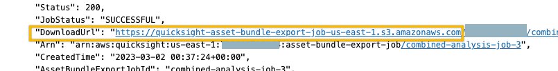
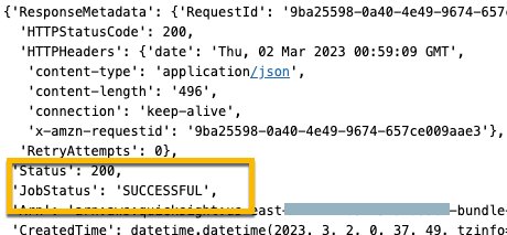


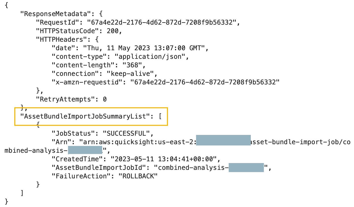
 Vetri Natarajan is a Specialist Solutions Architect for Amazon QuickSight. Vetri has 15 years of experience implementing enterprise business intelligence (BI) solutions and greenfield data products. Vetri specializes in integration of BI solutions with business applications and enable data-driven decisions.
 Zhao Pan is a software development manager for Amazon QuickSight. He is working to provide a delightful developer experience to our customers to automate and streamline their BI operations. He has 20 years of software development experience in various tech stacks. Prior to QuickSight he was a people and technical leader at ADP building a next-gen platform for human capital management. When he is not at his desk, he can usually be found in his garage building one contraption or another.
 Mayank Agarwal is a product manager for Amazon QuickSight, AWS’ cloud-native, fully managed BI service. He focuses on embedded analytics and developer experience. He started his career as an embedded software engineer developing handheld devices. Prior to QuickSight he was leading engineering teams at Credence ID, developing custom mobile embedded device and web solutions using AWS services that make biometric enrollment and identification fast, intuitive, and cost-effective for Government sector, healthcare and transaction security applications.

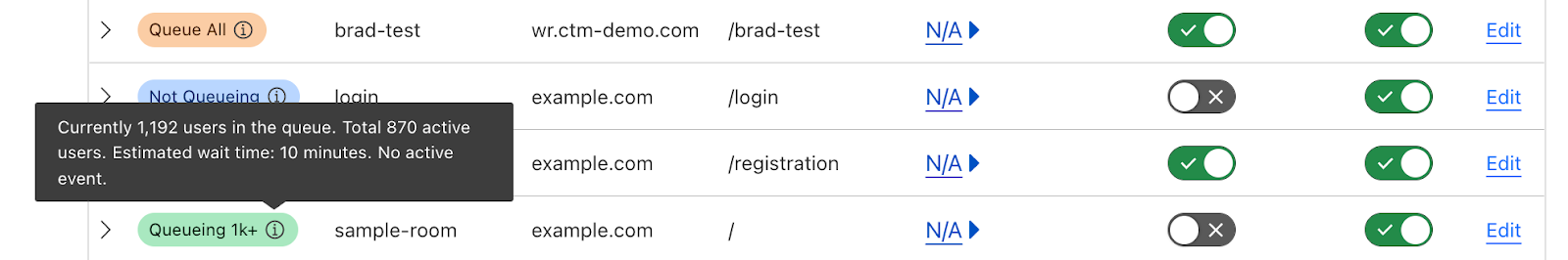
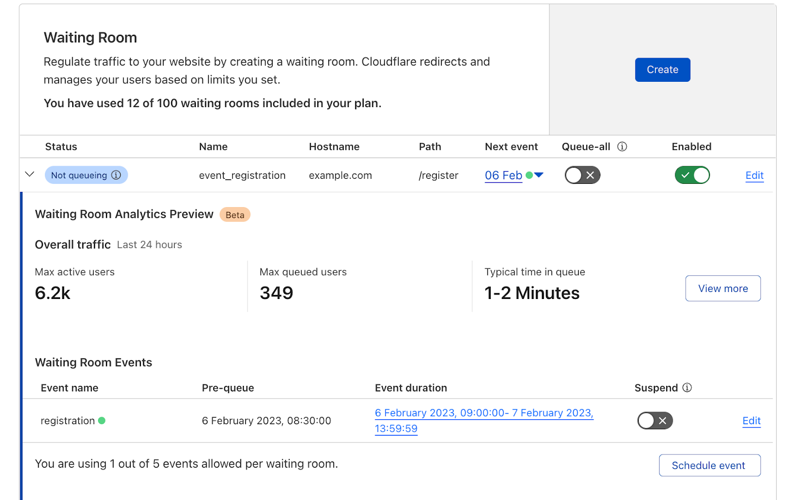

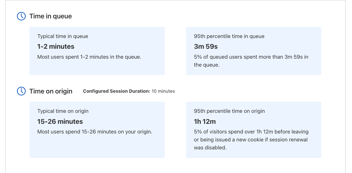
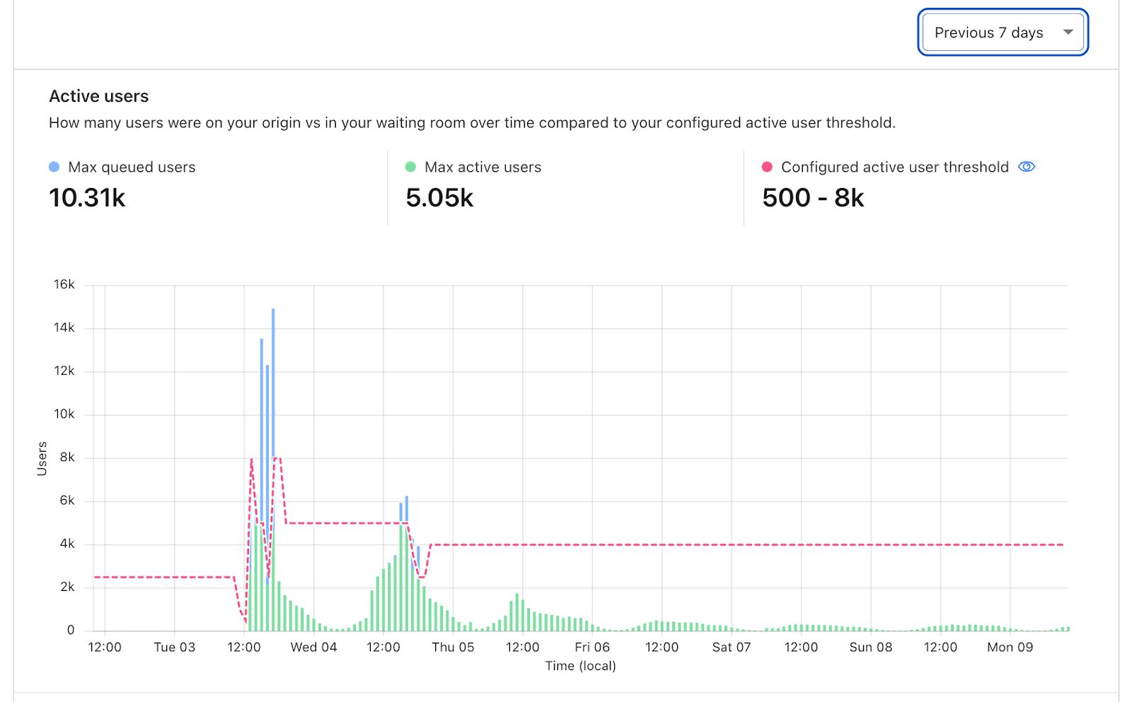
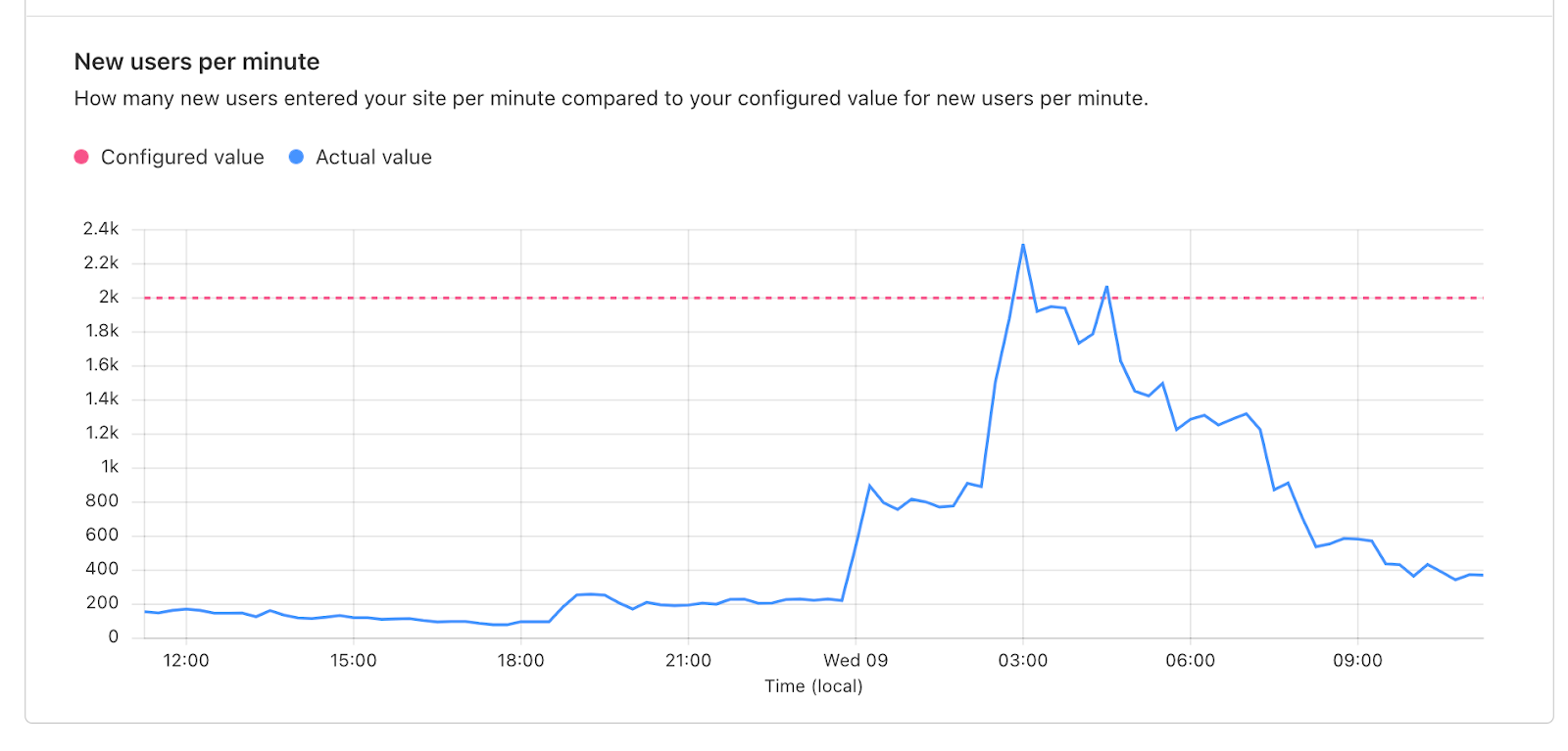
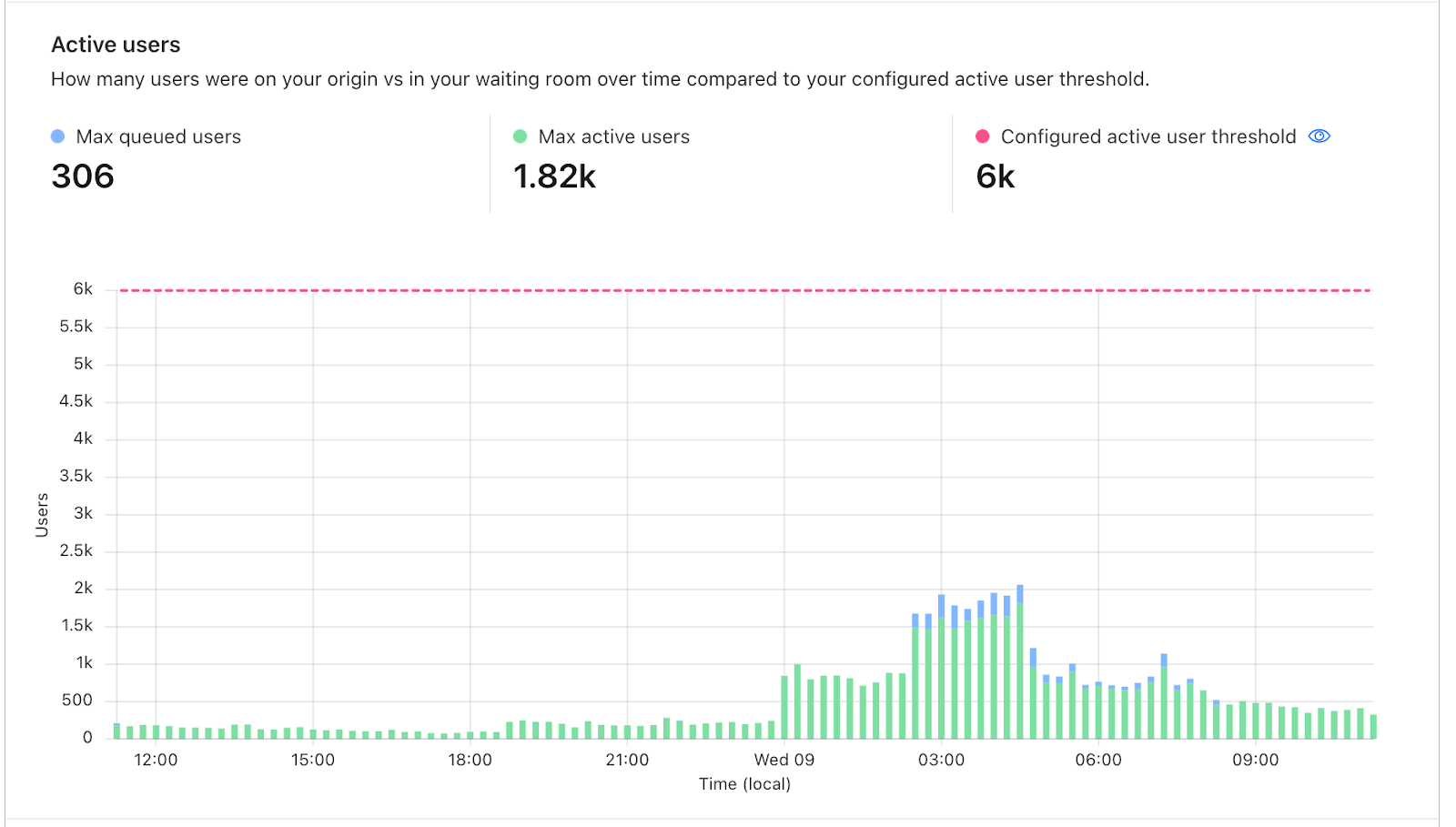
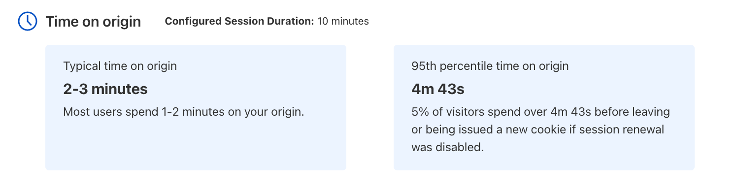
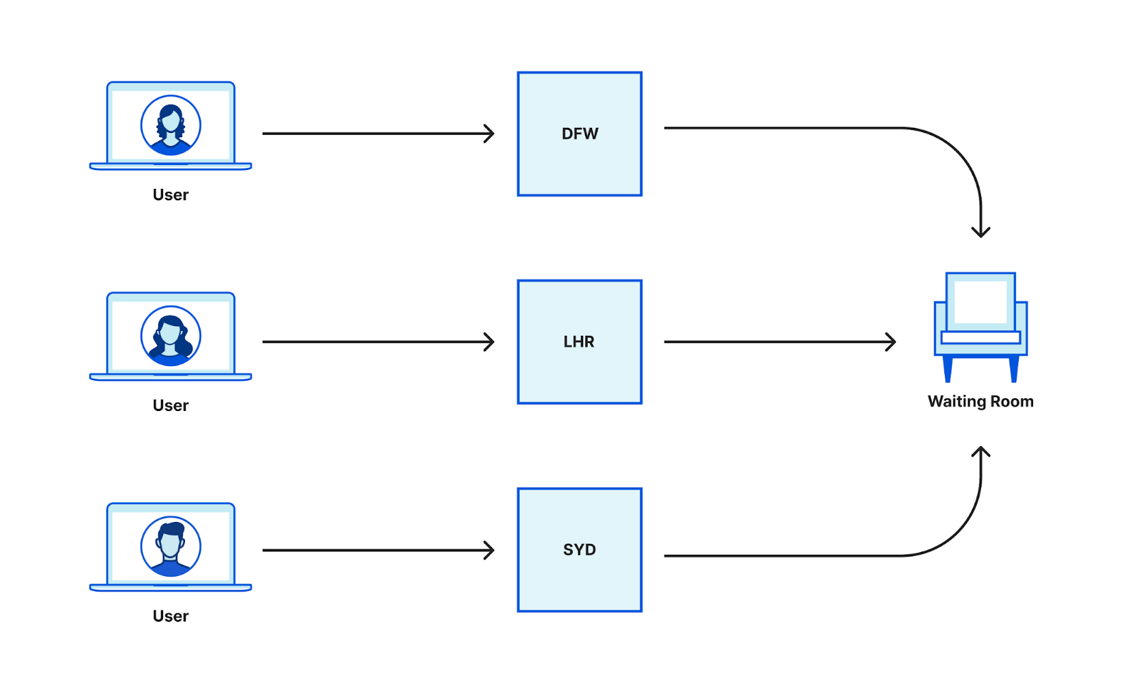
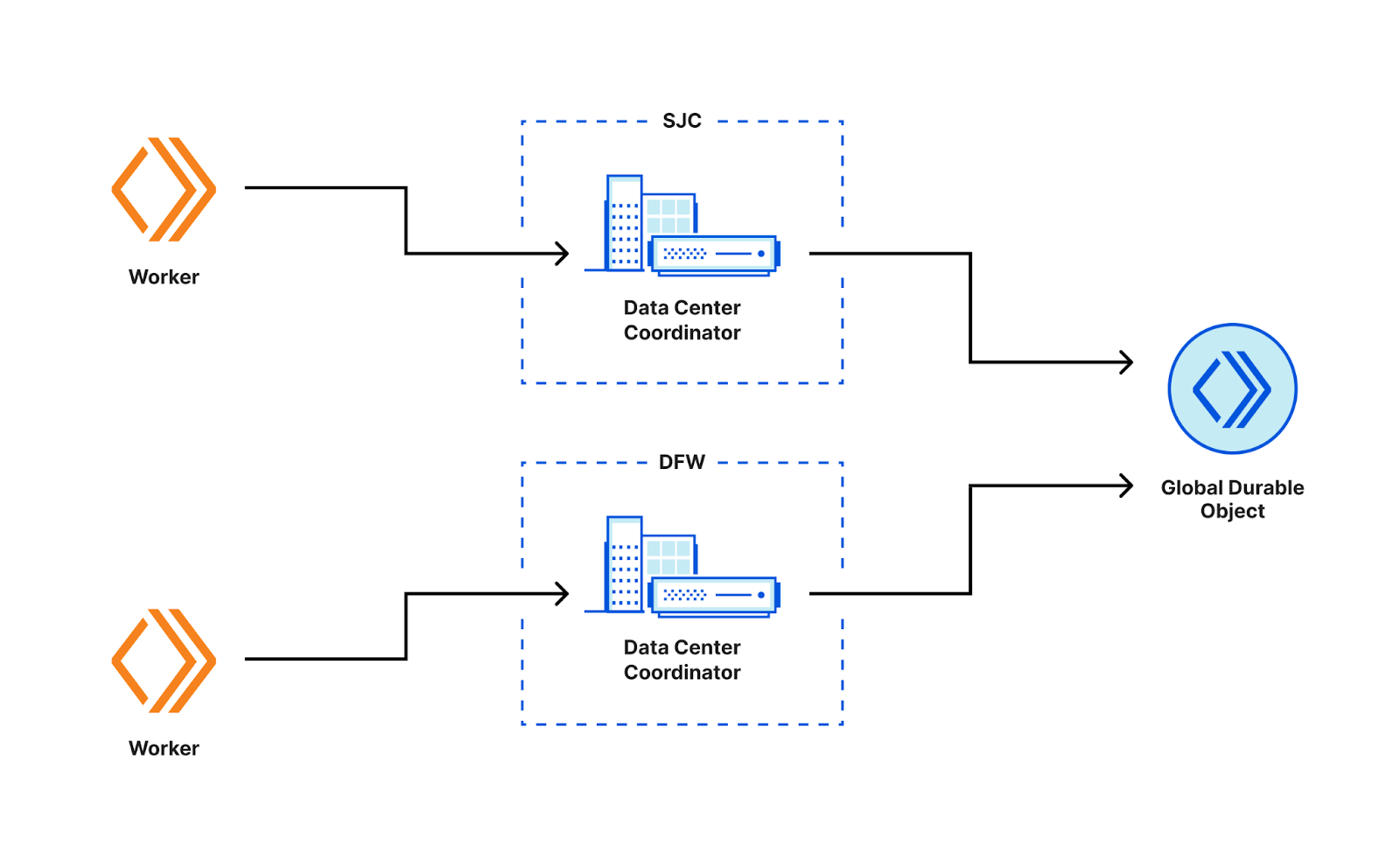

 Lotfi Mouhib is a Senior Solutions Architect working for the Public Sector team with Amazon Web Services. He helps public sector customers across EMEA realize their ideas, build new services, and innovate for citizens. In his spare time, Lotfi enjoys cycling and running.
 Vara Bonthu is a dedicated technology professional and Worldwide Tech Leader for Data on EKS, specializing in assisting AWS customers ranging from strategic accounts to diverse organizations. He is passionate about open-source technologies, data analytics, AI/ML, and Kubernetes, and boasts an extensive background in development, DevOps, and architecture. Vara’s primary focus is on building highly scalable data and AI/ML solutions on Kubernetes platforms, helping customers harness the full potential of cutting-edge technology for their data-driven pursuits.
 Tome Tanasovski is a Technical Manager at AWS, for a team that manages capabilities into Amazon’s big data platforms via AWS Glue. Prior to working at AWS, Tome was an executive for a market-leading global financial services firm in New York City where he helped run the Firm’s Artificial Intelligence & Machine Learning Center of Excellence. Prior to this role he spent nine years in the Firm focusing on automation, cloud, and distributed computing. Tome has a quarter-of-a-century worth of experience in technology in the Tri-state area across a wide variety of industries including big tech, finance, insurance, and media.
 Brian Ross is a Senior Software Development Manager at AWS. He has spent 24 years building software at scale and currently focuses on serverless data integration with AWS Glue. In his spare time, he studies ancient texts, cooks modern dishes and tries to get his kids to do both.


 Zack Zhou is a Software Development Engineer on the AWS Glue team.
 Avik Bhattacharjee is a Senior Partner Solutions Architect at AWS. He works with customers to build IT strategy, making digital transformation through the cloud more accessible, focusing on big data and analytics and AI/ML.
 Amit Kumar Panda is a Data Architect at AWS Professional Services who is passionate about helping customers build scalable data analytics solutions to enable making critical business decisions.


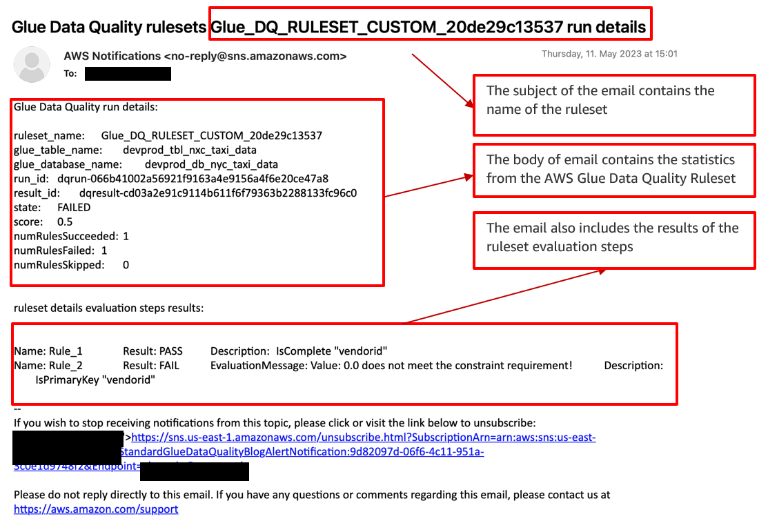
 Neel Patel is a software engineer working within GlueML. He has contributed to the AWS Glue Data Quality feature and hopes it will expand the repertoire for all AWS CloudFormation users along with displaying the power and usability of AWS Glue as a whole.
 Edward Cho is a Software Development Engineer at AWS Glue. He has contributed to the AWS Glue Data Quality feature as well as the underlying open-source project Deequ.


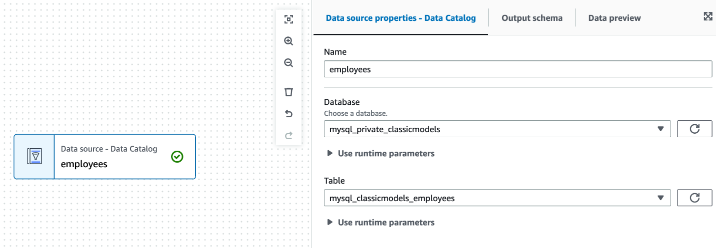


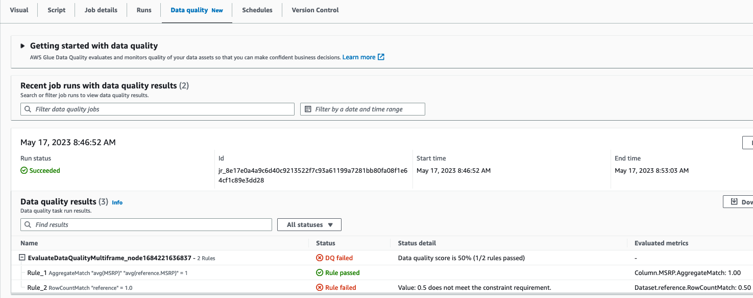


 Navnit Shukla is AWS Specialist Solutions Architect in Analytics. He is passionate about helping customers uncover insights from their data. He builds solutions to help organizations make data-driven decisions.
 Rahul Sharma is a Software Development Engineer at AWS Glue. He focuses on building distributed systems to support features in AWS Glue. He has a passion for helping customers build data management solutions on the AWS Cloud.
 Shriya Vanvari is a Software Developer Engineer in AWS Glue. She is passionate about learning how to build efficient and scalable systems to provide better experience for customers. Outside of work, she enjoys reading and chasing sunsets.

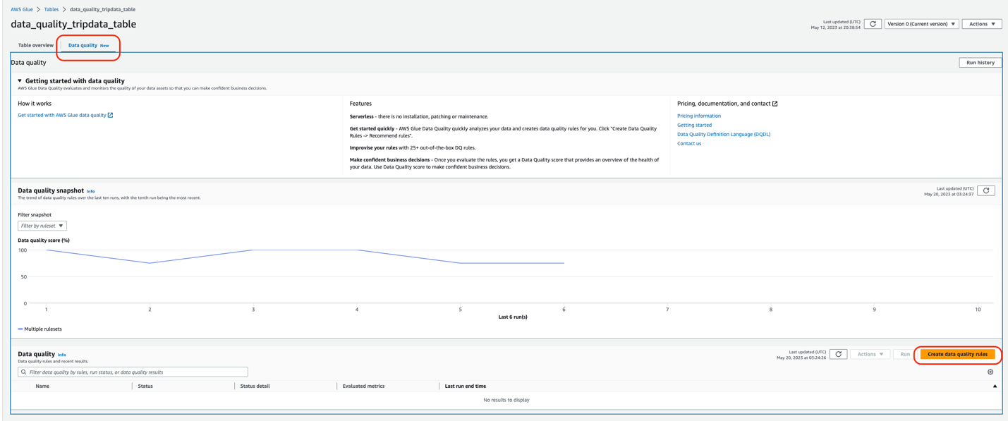


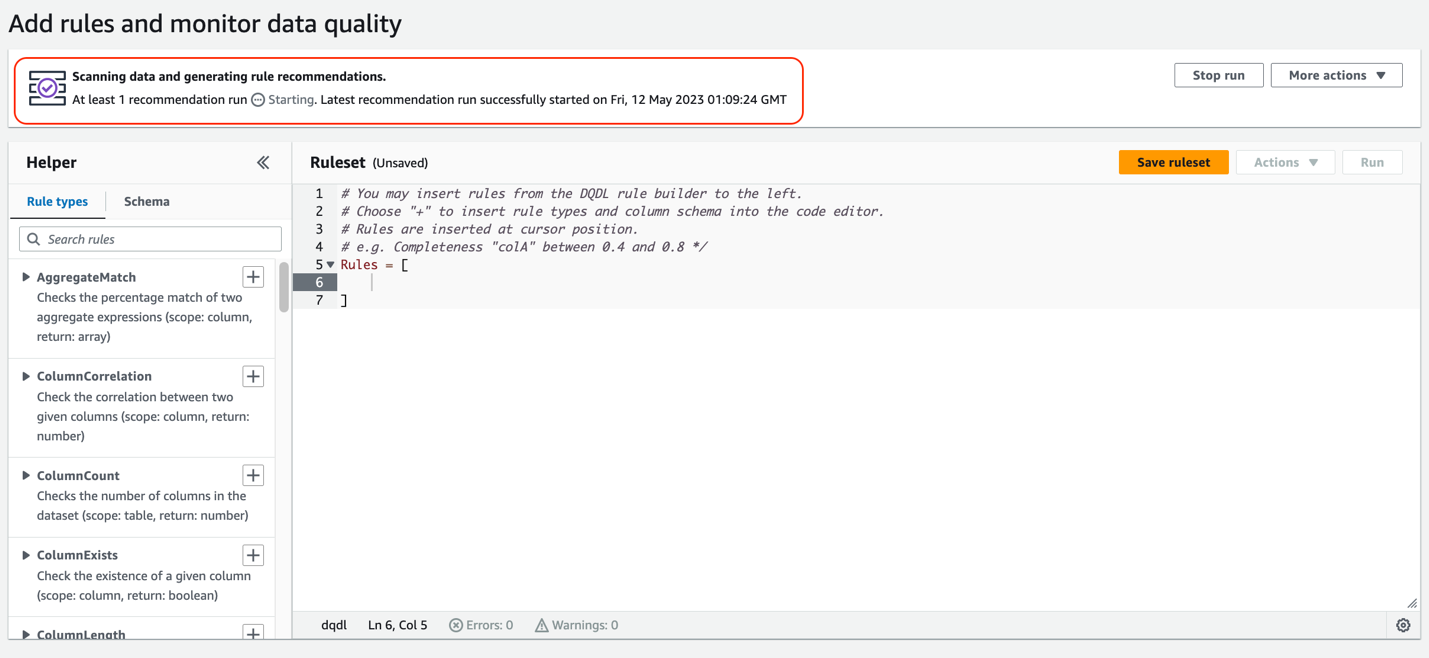

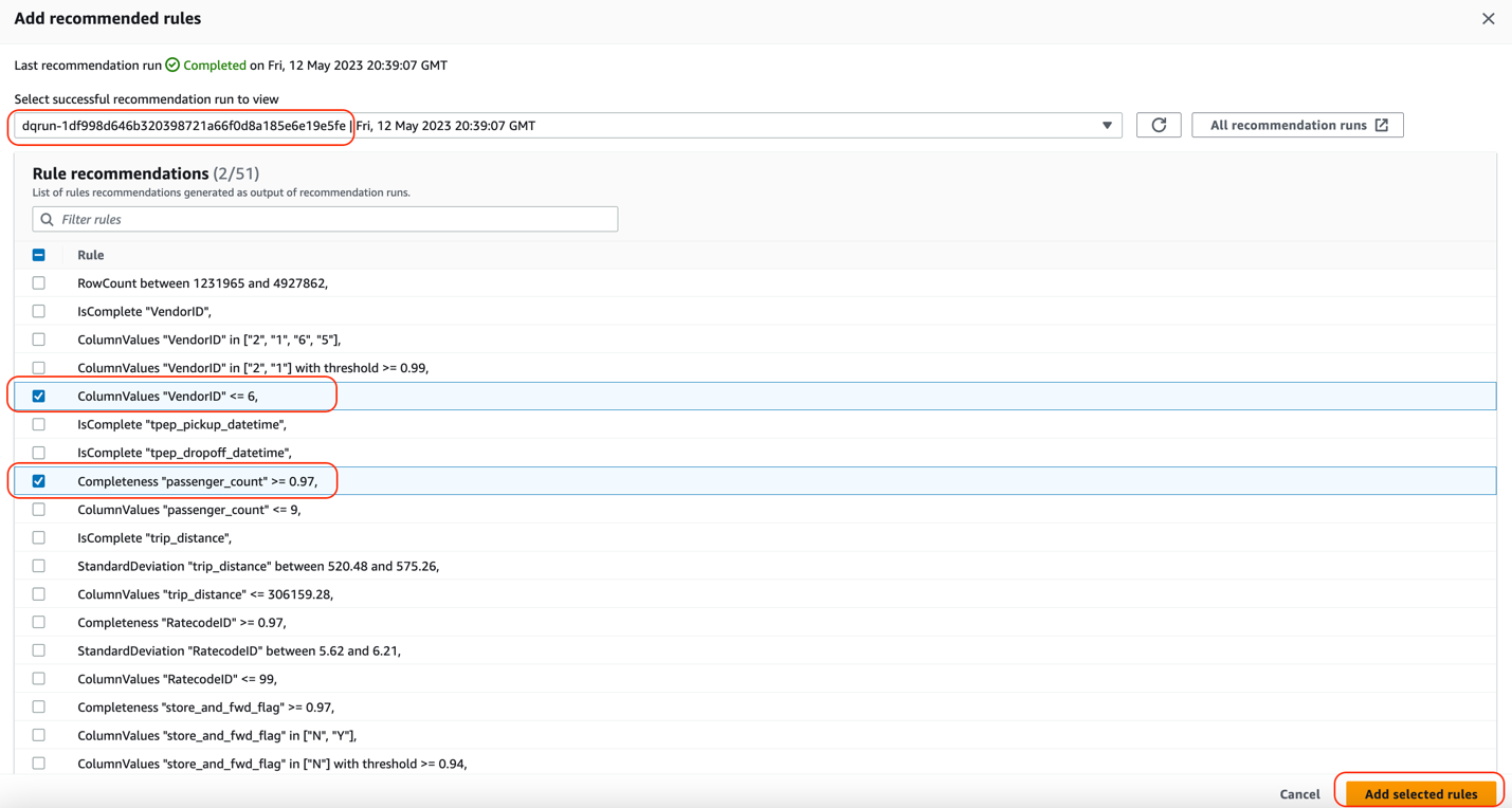
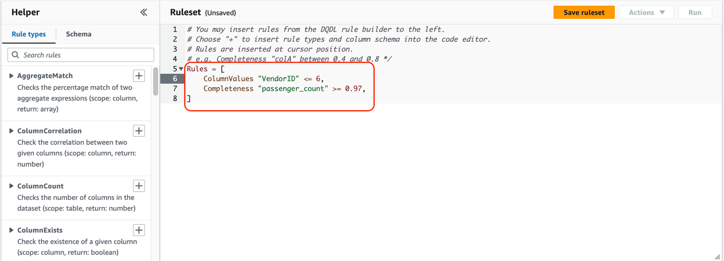


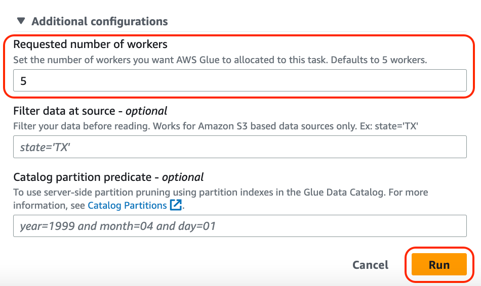


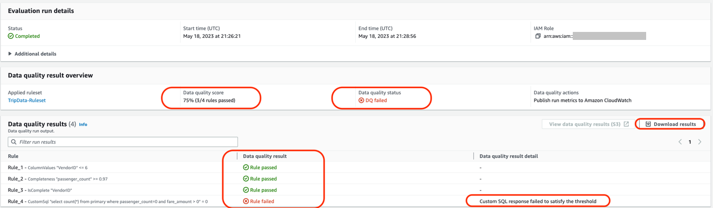
 Stuti Deshpande is an Analytics Specialist Solutions Architect at AWS. She works with customers around the globe, providing them strategic and architectural guidance on implementing analytics solutions using AWS. She has extensive experience in Big Data, ETL, and Analytics. In her free time, Stuti likes to travel, learn new dance forms, and enjoy quality time with family and friends.
 Aniket Jiddigoudar is a Big Data Architect on the AWS Glue team. He works with customers to help improve their big data workloads. In his spare time, he enjoys trying out new food, playing video games, and kickboxing.
 Joseph Barlan is a Frontend Engineer at AWS Glue. He has over 5 years of experience helping teams build reusable UI components and is passionate about frontend design systems. In his spare time, he enjoys pencil drawing and binge watching tv shows.
 Jesus Max Hernandez is a Software Development Engineer at AWS Glue. He joined the team in August after graduating from The University of Texas at El Paso. Outside of work, you can find him practicing guitar or playing softball in Central Park.
 Divya Gaitonde
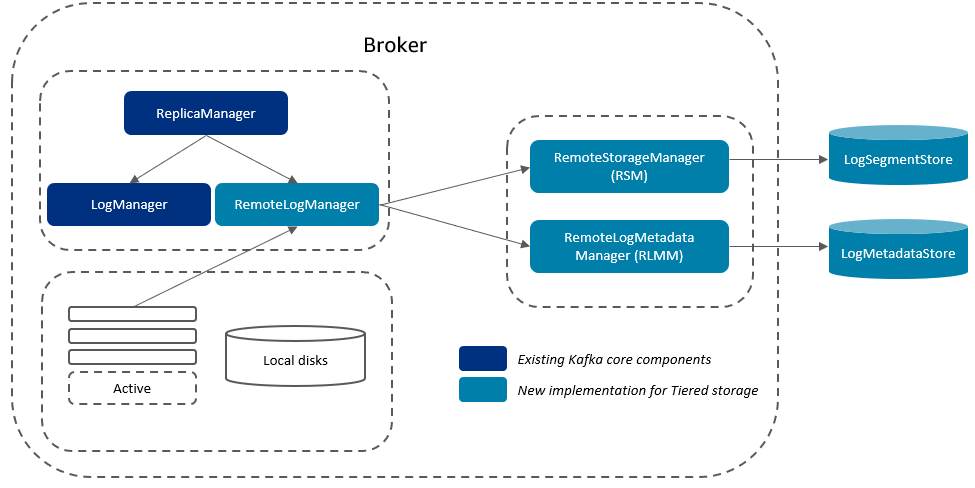
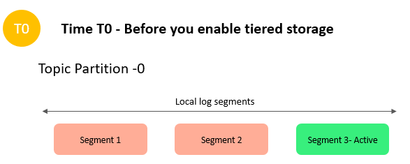
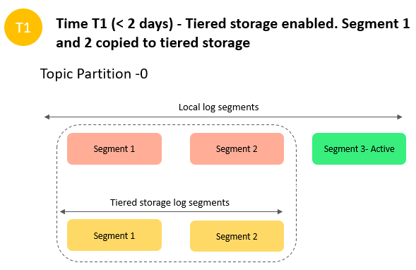
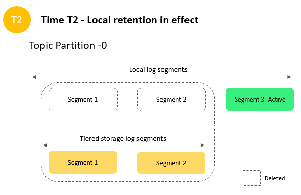

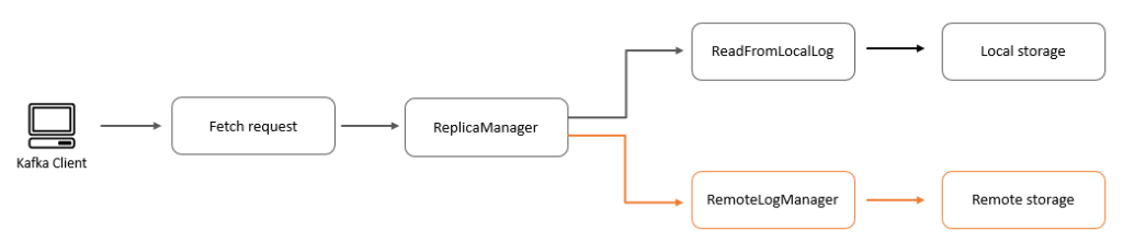
 Nagarjuna Koduru is a Principal Engineer in AWS, currently working for AWS Managed Streaming For Kafka (MSK). He led the teams that built MSK Serverless and MSK Tiered storage products. He previously led the team in Amazon JustWalkOut (JWO) that is responsible for realtime tracking of shopper locations in the store. He played pivotal role in scaling the stateful stream processing infrastructure to support larger store formats and reducing the overall cost of the system. He has keen interest in stream processing, messaging and distributed storage infrastructure.
 Masudur Rahaman Sayem is a Streaming Data Architect at AWS. He works with AWS customers globally to design and build data streaming architectures to solve real-world business problems. He specializes in optimizing solutions that use streaming data services and NoSQL. Sayem is very passionate about distributed computing.
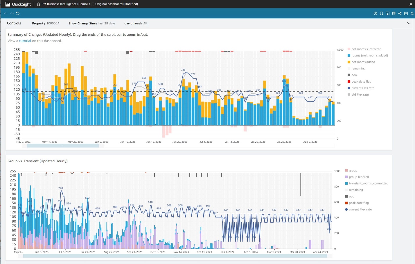
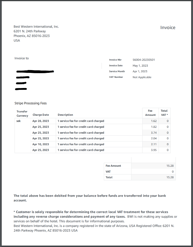
 Joseph W. Landucci serves as Director of Technology Management at BWH Hotels where he has spent over eight years building and evolving their data management strategy. In this role he is responsible for the management and strategic direction of six product teams: Database, Revenue Management Systems, Data Services, Loyalty Applications, Loyalty Automation and Enterprise Analytics.


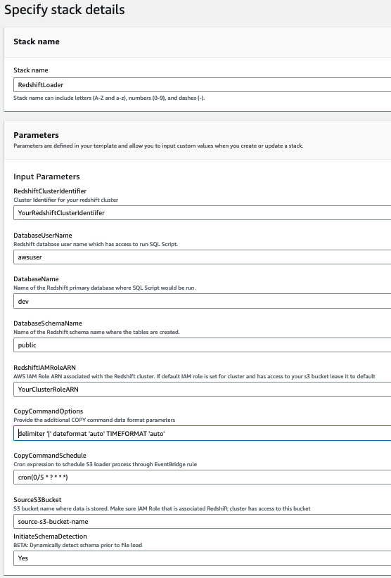
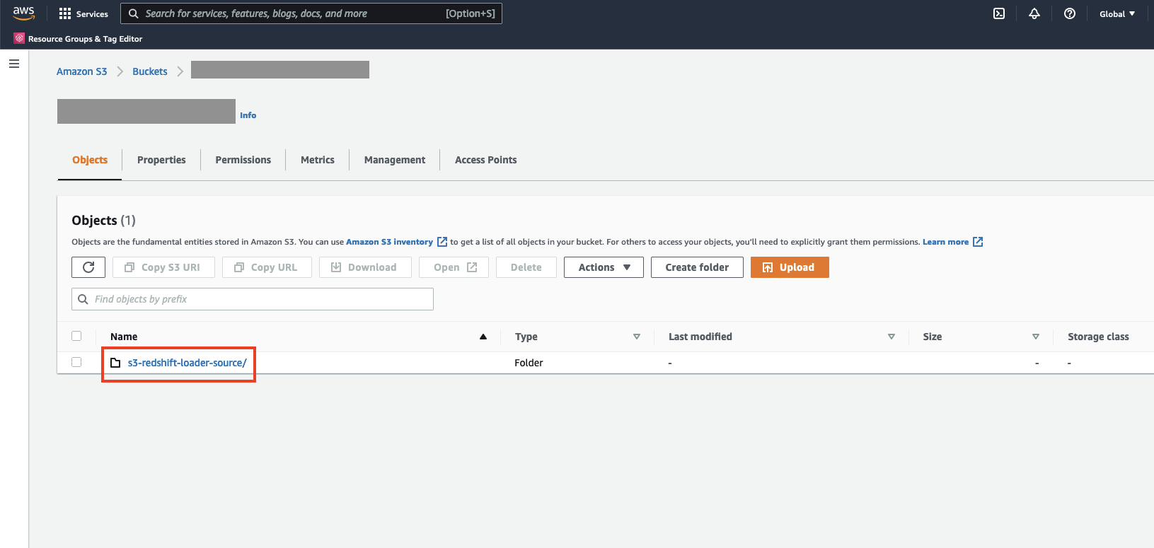

 Tahir Aziz is an Analytics Solution Architect at AWS. He has worked with building data warehouses and big data solutions for over 13 years. He loves to help customers design end-to-end analytics solutions on AWS. Outside of work, he enjoys traveling and cooking.
 Ritesh Kumar Sinha is an Analytics Specialist Solutions Architect based out of San Francisco. He has helped customers build scalable data warehousing and big data solutions for over 16 years. He loves to design and build efficient end-to-end solutions on AWS. In his spare time, he loves reading, walking, and doing yoga.
 Fabrizio Napolitano is a Principal Specialist Solutions Architect for DB and Analytics. He has worked in the analytics space for the last 20 years, and has recently and quite by surprise become a Hockey Dad after moving to Canada.
 Manjula Nagineni is a Senior Solutions Architect with AWS based in New York. She works with major financial service institutions, architecting and modernizing their large-scale applications while adopting AWS Cloud services. She is passionate about designing big data workloads cloud-natively. She has over 20 years of IT experience in software development, analytics, and architecture across multiple domains such as finance, retail, and telecom.
 Sohaib Katariwala is an Analytics Specialist Solutions Architect at AWS. He has over 12 years of experience helping organizations derive insights from their data.
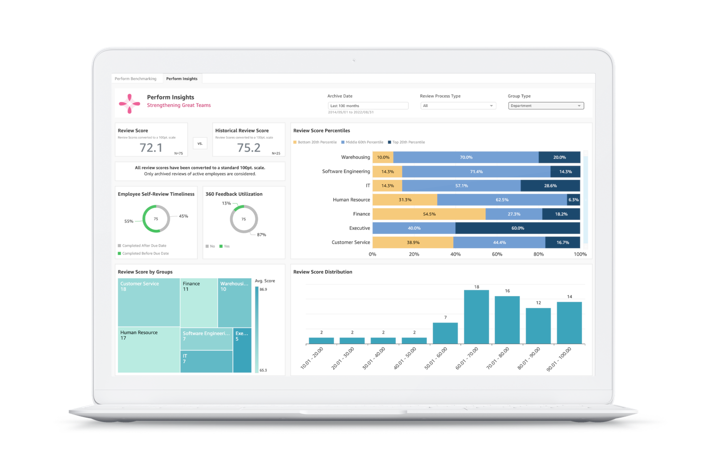
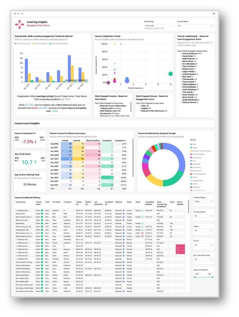
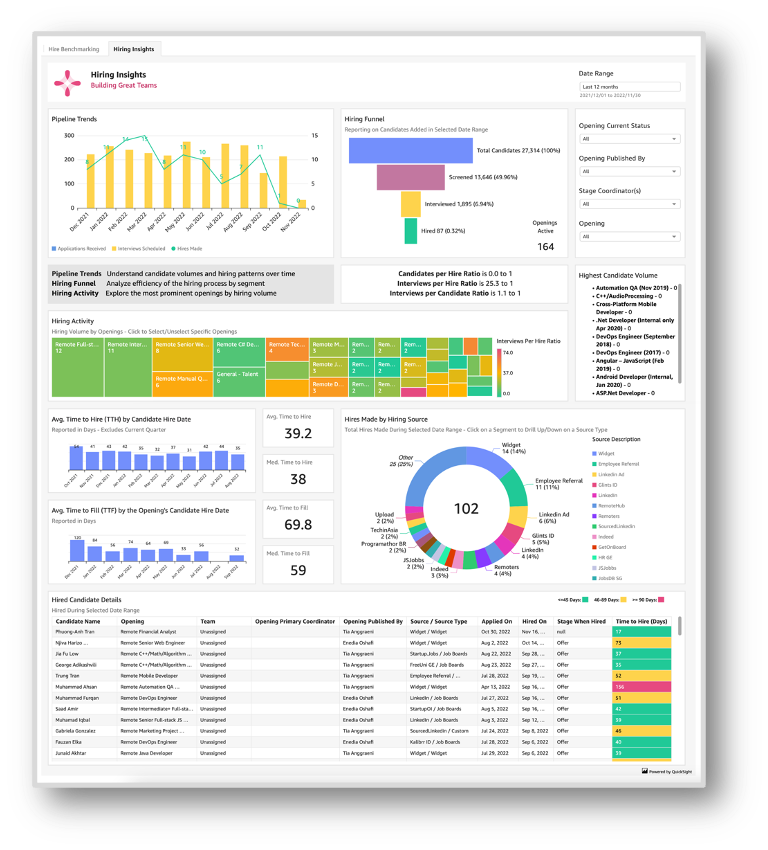
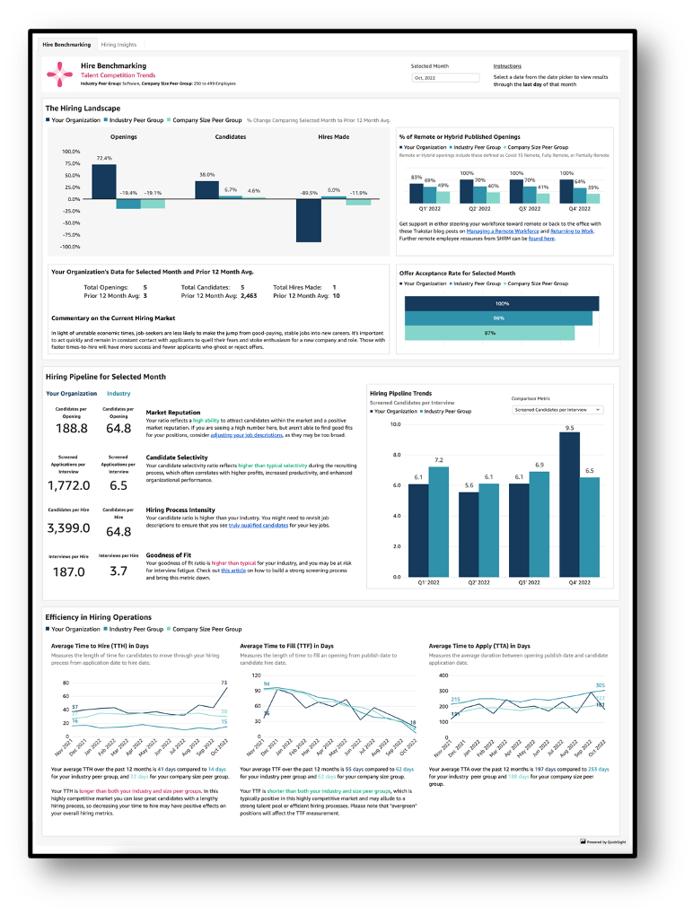

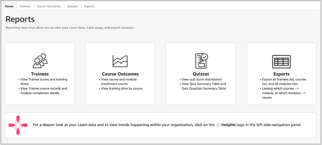
 Brian Kasen is the Director, Business Intelligence at Mitratech. He is passionate about helping HR leaders be more data-driven in their efforts to hire, retain, and engage their employees. Prior to Mitratech, Brian spent much of his career building analytic solutions across a range of industries, including higher education, restaurant, and software.
 Rebecca McAlpine is the Senior Product Manager for Trakstar Insights at Mitratech. Her experience in HR tech experience has allowed her to work in various areas, including data analytics, business systems optimization, candidate experience, job application management, talent engagement strategy, training, and performance management.
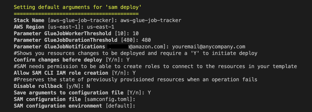

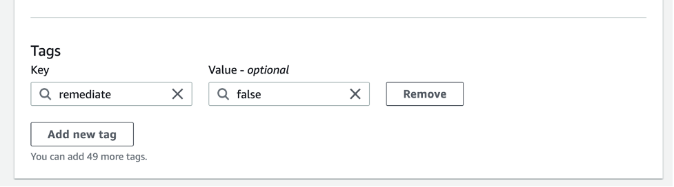
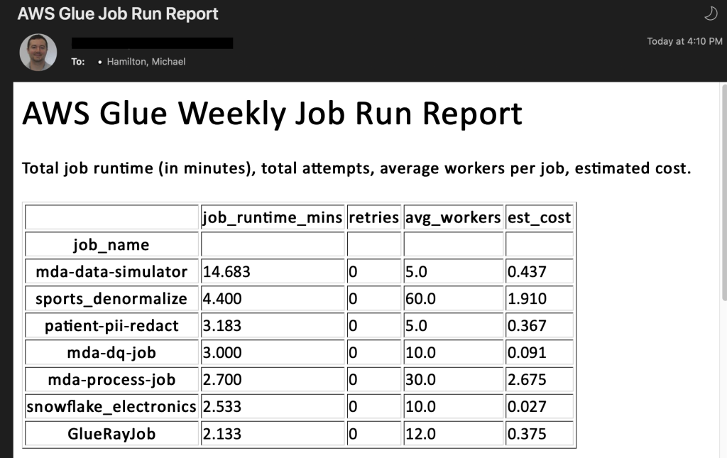
 Michael Hamilton is a Sr Analytics Solutions Architect focusing on helping enterprise customers in the south east modernize and simplify their analytics workloads on AWS. He enjoys mountain biking and spending time with his wife and three children when not working.
 Angus Ferguson is a Solutions Architect at AWS who is passionate about meeting customers across the world, helping them solve their technical challenges. Angus specializes in Data & Analytics with a focus on customers in the financial services industry.

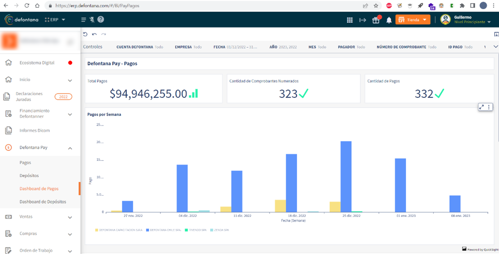
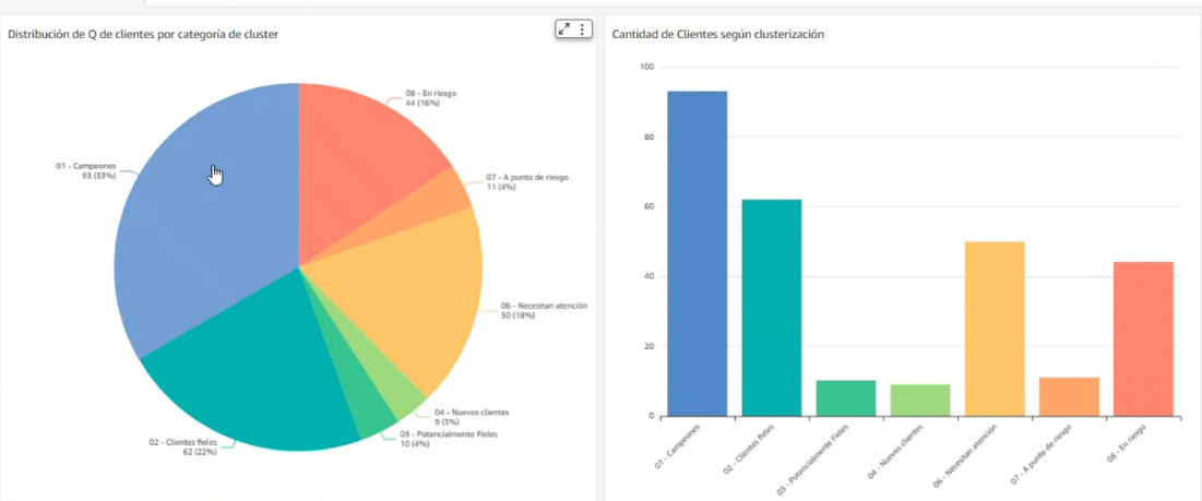
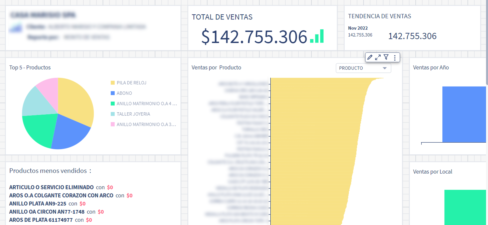
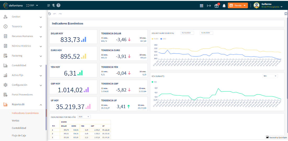
 Cynthia Valeriano is a Business Intelligence Developer of at Defontana, with skills focused on data analysis and visualization. With 3 years of experience in administrative areas and 2 years of experience in business intelligence projects, she has been in charge of implementing data migration and transformation tasks with various AWS tools, such as AWS DMS and AWS Glue, in addition to generating multiple dashboards in Amazon QuickSight.
 Jaime Olivares is a Senior software developer at Defontana, with 6 years of experience in the development of various technologies focused on the analysis of solutions and customer requirements. Experience with AWS in various services, including product development through QuickSight for the analysis of business and accounting data.
 Guillermo Puelles is a Technical Manager of the “Appia” Integrations team at Defontana, with 9 years of experience in software development and 5 years working with AWS tools. Responsible for planning and managing various projects for the implementation of BI solutions through QuickSight and other AWS services.


 Avijit Goswami is a Principal Solutions Architect at AWS specialized in data and analytics. He supports AWS strategic customers in building high-performing, secure, and scalable data lake solutions on AWS using AWS managed services and open-source solutions. Outside of his work, Avijit likes to travel, hike in the San Francisco Bay Area trails, watch sports, and listen to music.
 Rajarshi Sarkar is a Software Development Engineer at Amazon EMR/Athena. He works on cutting-edge features of Amazon EMR/Athena and is also involved in open-source projects such as Apache Iceberg and Trino. In his spare time, he likes to travel, watch movies, and hang out with friends.
 Prashant Singh is a Software Development Engineer at AWS. He is interested in Databases and Data Warehouse engines and has worked on Optimizing Apache Spark performance on EMR. He is an active contributor in open source projects like Apache Spark and Apache Iceberg. During his free time, he enjoys exploring new places, food and hiking.
 Antonio Vespoli is a Software Development Engineer in AWS. He works on Amazon Kinesis Data Analytics, the managed offering for running Apache Flink applications on AWS.
 Samuel Siebenmann is a Software Development Engineer in AWS. He works on Amazon Kinesis Data Analytics, the managed offering for running Apache Flink applications on AWS.
 Nuno Afonso is a Software Development Engineer in AWS. He works on Amazon Kinesis Data Analytics, the managed offering for running Apache Flink applications on AWS.
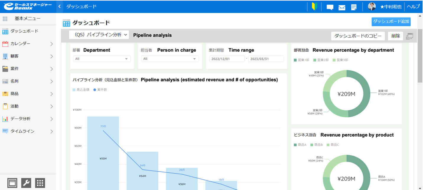

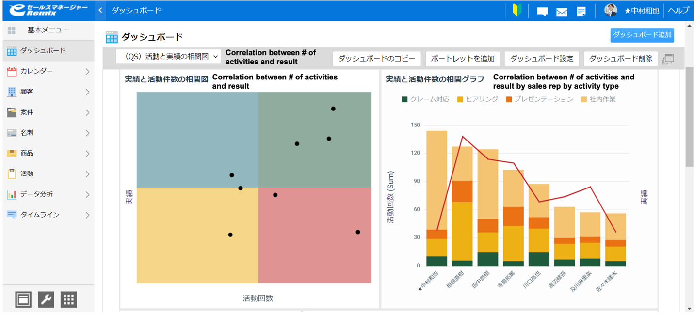
 Kenta Oda is the Chief Technology Officer at SOFTBRAIN Co., Ltd. He is in responsible of new product development with keen insight on better customer experience and go-to-market strategy.


 Manish Virwani is a Sr. Solutions Architect at AWS. He has more than a decade of experience designing and implementing large-scale big data and analytics solutions. He provides technical guidance, design advice, and thought leadership to some of the key AWS customers and partners.
 Indira Balakrishnan is a Principal Solutions Architect in the AWS Analytics Specialist SA Team. She is passionate about helping customers build cloud-based analytics solutions to solve their business problems using data-driven decisions. Outside of work, she volunteers at her kids’ activities and spends time with her family.


 Phil Goldstein is a copywriter and editor with AWS product marketing. He has 15 years of technology writing experience, and prior to joining AWS was a senior editor at a content marketing agency and a business journalist covering the wireless industry.

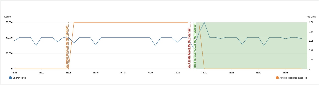


 Gaurav Bafna is a Senior Software Engineer working on OpenSearch at Amazon Web Services. He is fascinated about solving problems in distributed systems. He is a maintainer and an active contributor to OpenSearch.
 Murali Krishna is a Senior Principal Engineer at AWS OpenSearch Service. He has built AWS OpenSearch Service and AWS CloudSearch. His areas of expertise include Information Retrieval, Large scale distributed computing, low latency real time serving systems etc. He has vast experience in designing and building web scale systems for crawling, processing, indexing and serving text and multimedia content. Prior to Amazon, he was part of Yahoo!, building crawling and indexing systems for their search products.
 Ranjith Ramachandra is a Senior Engineering Manager working on Amazon OpenSearch Service. He is passionate about highly scalable distributed systems, high performance and resilient systems.