Post Syndicated from Bryan Van Hook original https://aws.amazon.com/blogs/security/centrally-manage-vpc-network-acl-rules-to-block-unwanted-traffic-using-aws-firewall-manager/

Amazon Virtual Private Cloud (Amazon VPC) provides two options for controlling network traffic: network access control lists (ACLs) and security groups. A network ACL defines inbound and outbound rules that allow or deny traffic based on protocol, IP address range, and port range. Security groups determine which inbound and outbound traffic is allowed on a network interface, but they cannot explicitly deny traffic like a network ACL can. Every VPC subnet is associated with a network ACL that ultimately determines which traffic can enter or leave the subnet, even if a security group allows it. Network ACLs provide a layer of network controls that augment your security groups.

There are situations when you might want to deny specific sources or destinations within the range of network traffic allowed by security groups. For example, you want to deny inbound traffic from malicious sources on the internet, or you want to deny outbound traffic to ports or protocols used by exploits or malware. Security group rules can only control what traffic is allowed. If you want to deny specific traffic within the range of allowed traffic from security groups, you need to use network ACL rules. If you want to deny specific types of traffic in many VPCs, you need to update each network ACL associated with subnets in each of those VPCs. We heard from customers that implementing a baseline of common network ACL rules can be challenging to manage across many Amazon Web Services (AWS) accounts, so we expanded AWS Firewall Manager capabilities to make this easier.

AWS Firewall Manager network ACL security policies allow you to centrally manage network ACL rules for VPC subnets across AWS accounts in your organization. The following sections demonstrate how you can use network ACL policies to manage common network ACL rules that deny inbound and outbound traffic.

Deny inbound traffic using a network ACL security policy

If you have not already set up a Firewall Manager administrator account, see Firewall Manager prerequisites. Note that network ACL policies require your AWS Config configuration recorder to include the AWS::EC2::NetworkAcl and AWS::EC2::Subnet resource types.

Let’s review an example of how you can now use Firewall Manager to centrally manage a network ACL rule that denies inbound traffic from a public source IP range.

To deny inbound traffic:

1. Sign in to your Firewall Manager delegated administrator account, open the AWS Management Console, and go to Firewall Manager.
2. In the navigation pane, under AWS Firewall Manager, select Security policies.
3. On the Filter menu, select the AWS Region where your VPC subnets are defined, and choose Create policy. In this example, we select US East (N. Virginia).
4. Under Policy details, select Network ACL, and then choose Next.
   

   Figure 1: Network ACL policy type and Region

5. On Policy name, enter a Policy name and Policy description.
   

   Figure 2: Network ACL policy name and description

6. In the Network ACL policy rules section, select the Inbound rules tab.
7. In the First rules section, choose Add rules.
   

   Figure 3: Add rules in the First rules section

8. In the Inbound rules window, choose Add inbound rules.
   

   Figure 4: Add inbound rules

9. For Inbound rules, choose the following:
   1. For Type, select All traffic.
   2. For Protocol, select All.
   3. For Port range, select All.
   4. For Source, enter an IP address range that you want to deny. In this example, we use 192.0.2.0/24.
   5. For Action, select Deny.
   6. Choose Add Rules.
   

   Figure 5: Configure a network ACL inbound rule

10. In Network ACL policy rules, under First rules, review the deny rule.
    

    Figure 6: Review the inbound deny rule

11. Under Policy action, select the following:
    1. Select Auto remediate any noncompliant resources.
    2. Under Force Remediation, select Force remediate first rules. Firewall Manager compares your existing network ACL rules with rules defined in the policy. A conflict exists if a policy rule has the opposite action of an existing rule and overlaps with the existing rule’s protocol, address range, or port range. In these cases, Firewall Manager will not remediate the network ACL unless you enable force remediation.
    

    Figure 7: Configure the policy action

12. Choose Next.
13. Policy scope, select the following:
    1. Under AWS accounts this policy applies to, select the scope of accounts that apply. In this example, we include all accounts.
    2. Under Resource type, select Subnet.
    3. Under Resources, select the scope of resources that apply. In this example, we only include subnets that have a particular tag.
    

    Figure 8: Configure the policy scope

14. Enable resource cleanup if you want Firewall Manager to remove the rules it added to network ACLs associated with subnets that are no longer in scope. To enable cleanup, select Automatically remove protections from resources that leave the policy scope, and choose Next.
    

    Figure 9: Enable resource cleanup

15. Under Configure policy tags, define the tags you want to associate with your policy, and then choose Next.
16. Under Review and create policy, choose Next.

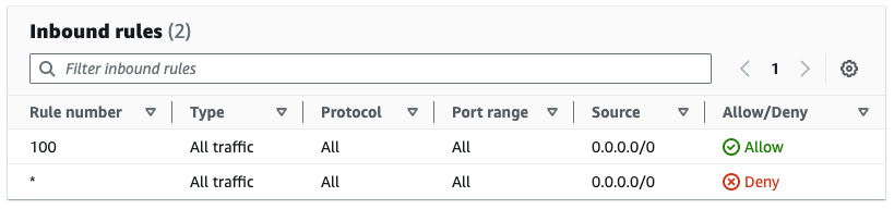
Before creating the Firewall Manager policy, the subnet is associated with a default network ACL, as shown in Figure 10.

Figure 10: Default network ACL rules before the subnet is in scope

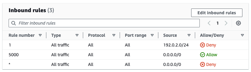
As shown in Figure 11, the subnet is now associated with a network ACL managed by Firewall Manager. The original Allow rule has been preserved and moved to priority 5,000. The Deny rule has been added with priority 1.

Figure 11: Inbound rules in network ACL managed by Firewall Manager

Deny outbound traffic using a network ACL security policy

You can also use Firewall Manager to implement outbound network ACL rules to deny the use of ports used by malware or software vulnerabilities. In this example, we’re blocking the use of LDAP port 389.

1. Sign in to your Firewall Manager delegated administrator account and open the Firewall Manager console.
2. In the navigation pane, under AWS Firewall Manager, select Security policies.
3. On the Filter menu, select the AWS Region where your VPC subnets are defined, and choose Create policy. In this example, we select US East (N. Virginia).
4. Under Policy details, select Network ACL, and then choose Next.
5. Enter a Policy name and Policy description.
6. In the Network ACL policy rules section, select the Outbound rules tab.
7. In the First rules section, choose Add rules.
   

   Figure 12: Add rules in the First rules section

8. Under Outbound rules, choose Add outbound rules.
9. In Outbound rules, select the following:
   1. For Type, select LDAP (389).
   2. For Destination, enter 0.0.0.0/0.
   3. For Action, select Deny.
   4. Choose Add Rules.
   

   Figure 13: Configure a network ACL outbound rule

10. On the Network ACL policy rules page, under First rules, review the deny rule.
    

    Figure 14: Review the outbound deny rule

11. In Policy action, under Policy action, select the following:
    1. Select Auto remediate any noncompliant resources.
    2. Under Force Remediation, select Force remediate first rules, and then choose Next.
    

    Figure 15: Configure the policy action

12. Under Policy scope, choose the following:
    1. Under AWS accounts this policy applies to, select the scope of accounts that apply. In this example, we include all accounts by selecting Include all accounts under my organization.
    2. Under Resource type, select Subnet.
    3. Under Resources, select the scope of resources that apply. In this example, we select Include only subnets that all the specified resource tags.
    

    Figure 16: Configure the policy scope

13. On Resource cleanup, enable resource cleanup if you want Firewall Manager to remove rules it added to network ACLs associated with subnets that are no longer in scope. To enable resource cleanup, select Automatically remove protections from resources that leave the policy scope, and then choose Next.
    

    Figure 17: Enable resource cleanup

14. Under Configure policy tags, define the tags you want to associate with your policy, and then choose Next.
15. Under Review and create policy, choose Next.

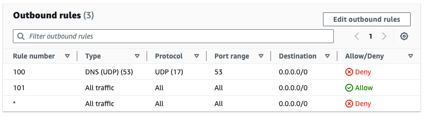
Before creating the Firewall Manager policy, the subnet is associated with a network ACL that already contains rules with priority 100 and 101, as shown in Figure 18.

Figure 18: Rules in original network ACL

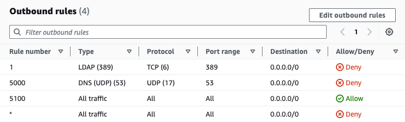
As shown in Figure 19, the subnet is now associated with a network ACL managed by Firewall Manager. The original rules have been preserved and moved to priority 5,000 and 5,100. The Deny rule for LDAP has been added with priority 1.

Figure 19: Outbound rules in network ACL managed by Firewall Manager

Working with network ACLs managed by Firewall Manager

Firewall Manager network ACL policies allow you to manage up to 5 inbound and 5 outbound rules. Network ACLs can support a total of 20 inbound rules and 20 outbound rules by default. This limit can be increased up to 40 inbound rules and 40 outbound rules, but network performance might be impacted. Consider AWS Network Firewall if you need support for more rules and a broader set of features.

To diagnose overly restrictive network ACL rules, see Querying Amazon VPC flow logs to learn more about using Amazon Athena to analyze your VPC flow logs.

AWS accounts that are in scope of your Firewall Manager policy might have identities with permission to modify network ACLs created by Firewall Manager. You can use a service control policy (SCP) to deny AWS Identity and Access Management (IAM) actions that modify network ACLs if you want to make sure that they are exclusively managed by Firewall Manager. Firewall Manager uses service-linked roles, which are not restricted by SCPs. The following example SCP denies network ACL updates without restricting Firewall Manager:

{
  "Version": "2012-10-17",
  "Statement": [
    {
      "Sid": "DenyNaclUpdateExceptFMS",
      "Effect": "Deny",
      "Action": [
        "ec2:CreateNetworkAclEntry",
        "ec2:DeleteNetworkAclEntry",
        "ec2:ReplaceNetworkAclAssociation",
        "ec2:ReplaceNetworkAclEntry"
      ],
      "Resource": "*"
    }
  ]
}

Summary

Prior to AWS Firewall Manager network ACL security policies, you had to implement your own process to orchestrate updates to network ACLs across VPC subnets in your organization in AWS Organizations. AWS Firewall Manager network ACL security policies allow you to centrally define common network ACL rules that are automatically applied to VPC subnets across your organization, even as you add new accounts and resources. In this post, we demonstrated how you can use network ACL policies in a variety of scenarios, such as blocking ingress from malicious sources and blocking egress to destinations used by malware and exploits. You can also use network ACL policies to implement an allow list. For example, you might only want to allow egress to your on-premises network.

To get started, explore network ACL security policies in the Firewall Manager console. For more information, see the AWS Firewall Manager Developer Guide and send feedback to AWS re:Post for AWS Firewall Manager or through your AWS support team.