Фразата от стихотворение на Борис Христов беше мотото на заключителния сезон на тазгодишните есенни Литературни срещи. Трийсет и пет години след падането на Берлинската стена, употребата на минало време (бе, беше) би фиксирало само историческия факт.
Дали културните разломи не се разширяват отново? Хибридната война, виртуалните ни стени, акустиката в приятелските кръгове – усещаме ли изобщо кога e преминат собственият ни Checkpoint Charlie?
Символизираното от Стената разделение провокира нови поводи за разговор. Вече не толкова по оста Изток–Запад, все още уместна впрочем. А поради разширяващите се като концентрични кръгове конотации на идеята за сепариране – като опит да се самоопределим.
И докато ограждането със стени е един от древните модели да защитиш и отграничиш своето, полиса, цивилизованото пространство, то днес човек започва да се пита как функционира (споменът за) Берлинската стена, която разполови един град, прерязвайки семейни връзки, улици, дори и няколко къщи.
В официалното ѝ наименование на немски фигурира Schutzwall ‘защитна стена, ров’.
Стената, от двете страни на която се говори един език. Макар през годините той да обраства с различни идеологеми.
Стената като бариера.
Стената като инструмент.
Стената като охранявана граница, която разполовява тялото на Европа на Източна и Западна. И на която се стреля на месо. Като че ли човекът може да бъде само месо.
И от двете страни на Берлинската стена имаше цивилизации. И двете имаха основанията и инструментариума да асоциират света отсреща с другост. Другостта като враг, привкусът на хтонично, заплашително пространство. Институционализирането на страха от нашата, източната страна на Стената – нека признаем – го правеше още по-жив.
Падането на Берлинската стена беше не просто опит за интегриране, а кредо, символ верую. Изповядване на увереността, че можем да живеем в единение. Заедно.
Трийсет и пет години по-късно (което е около поколение и малко) никой вече няма желание за илюзии. Защитните ровове се множат и местят като в игра на тетрис. Стената обаче се превърна в повод за диалогизиране. В метафора, която функционира отвъд полето на идеологемите – като опит да разберем кои сме и защо имаме толкова отчаяна нужда да се самоопределяме чрез разграничаването си от останалите.
По време на Литературните срещи деликатно, но много настойчиво беше поставен въпросът „Колко стени бяха издигнати, докато празнувахме падането на една от тях?“. (Да припомним и участниците в трите вечери: Джаки Томе, Надежда Радулова, Михаил Зигар, Георги Господинов, Катя Петровская, Йоанна Елми, Стефан Иванов, Пламен Дойнов, Оля Стоянова, Илко Димитров, Мирела Иванова, Еми Барух, Петър Чухов, Здравка Евтимова.)
Инсталацията в One Gallery (визуална идентичност – Костадин Кокаланов, студио FRANK) съдържаше текстове на Йоанна Елми и Стефан Иванов, писани по пет основни теми: самота, тъга, емиграция, носталгия, аномия. Да, акроним са на:
с
т
е
н
а
Самота
Мъртвите зони вътре в нас, в които я укриваме, са подобни на граничните територии – ничия земя, практически недостъпна. Поле, което семантично принадлежи на стената. Йоанна Елми неслучайно я свързва със страха:
… страх ме е и мен, ужасно ме е страх, че вече измерихме света, обиколихме го, завладяхме го, изядохме го, изцедихме го, изсушихме го, видяхме го да виси като синя ябълка в безкрайната градина на космоса, вече знаем колко сме малки.
Да, метафората на стената продължава да ражда асоциации с изолация и контролно-пропускателни пунктове. Дори да говорим за „стените“ си във Facebook – там, където почти две десетилетия човечеството обявява споделената си самота.
Синхронично Стефан Иванов също обвързва самотата с криза на идентичността и страх. Но и с дълбоките екзистенциални липси, които не ни позволяват да се чувстваме свързани с другите. А скрито и непреодолимо – и със себе си:
Как съм дълбал с ключ стената на съблекалнята. […] Затова пиша, за да съм чут и видян, за да прескоча и махна стената от тормоз, безразличие и юркане.
И отново сме там – при стената, която охранява собствената ни самота. Малката ни човешка самота („Болко, болкоо, болчице!“, беше възкликнал Ал. Геров) – понеже отвън е другото, неопитоменото, заплашителното.
Тъга
Тя е там, на ръба на безсилието, от другата страна на утехата. Призракът на стената тук е омекотен, одомашнен, понятен.
Не е нужно от тъгата да се прави фетиш, идол или табу,
пише Стефан Иванов. Подобна беше и дискретната нишка, прокарана в разговора между Катя Петровская и Георги Господинов (в книгите и на двамата им невъзможността да достигнеш не е непременно невъзможност да се свържеш емоционално с помощта на спасителната мисия на приемането).
Впрочем именно в Берлин живее Катя Петровская, а Михаил Зигар казва, че е между Берлин и Ню Йорк (обединения Берлин, в който споменът за Стената е белег от рана). Днес имаме възможност да правим подобен избор. Между 13 август 1961-ва и 9 ноември 1989 г. Стената е непроницаема и охранявана граница между двете германски държави.
Дългите стени на тъгата неизбежно ни отвеждат и към онази молитвена варовикова стена, висока двайсет метра – Стената на плача. Защото надеждата е необходимата друга страна, не непременно противоположна на тъгата. Йоанна Елми в скоби си припомня, че е била на различни места, на които
пишеш желание на листче, навиваш го и го пъхаш между камъните.
И че понякога тя чете тези послания, пропъхнати в какви ли не стени, обикновено по свети места. Единени сме в тъгите си. В болката по невъзвратимото и липсващото.
Емиграция
Точно в центъра на стЕна-та. Като разрив, но и (най-сетне) като възможност. Свободен избор. Опит, отказван на няколко поколения от Източния блок. Хора, които са „предпазвани“ от нахлуващия от Запад морален разпад, както твърди пропагандата. За демонизирането на другия винаги се използва етичен наратив (реториката на националистическите партии, „Движение за изправяне на нравите“ – кампанията, започнала през 40-те години в Китай, печалното известните тук репресии, свързани с комунистическия морал). Не, границите не пазят затворените зад тях от прииждащо зло, те ултимативно не позволяват на хората от социалистическите страни да напуснат. И това не бива да бъде забравяно.
Мечтаните модели се оказват отвън, зад охраняваните стени на „полиса“. Варварите, да, също и онези от стихотворението на Кавафис „В очакване на варварите“, няма да нахлуят. Защото няма нищо желано, заради което да си струва.
И ето ни днес:
свършиха религиите, идеологиите, свърши и Запада, свършиха нещата, в които да се вярва. (Йоанна Елми)
Но нали човекът първом и винаги е емигрирал в себе си. Поради по-обхватния ужас, онзи отвъд конкретните исторически обстоятелства. Стефан Иванов го описва така:
Представял съм си, че вече няма заради кого да съм в тази държава […], че няма нищо, което да ме задържа, че мога да започна отначало и не, това не ме окуражаваше, а ме плашеше.
Иначе чисто житейски Йоанна Елми живее в САЩ, Стефан Иванов – в България. Дели ги един океан. Събира ги и литературната инсталация „С.Т.Е.Н.А.“.
Днес идеята за емиграция е примирима в общото виртуално пространство, което обитаваме по своя воля. Струва ми се обаче, че има едно място, от което никога не бихме успели да си тръгнем докрай. Езикът.
Носталгия
… светът, за който сме отгледани, вече не съществува, толкова много настояще, толкова много минало, никакво бъдеще… (Йоанна Елми)
Етимологично думата се свързва с „тъгата, болката по дома“, по загубеното, напоследък – с горчиво-сладкия копнеж по невъзвратимото. Помня, помня, изброява Стефан Иванов в текста си за „Стена“-та: одеяло, бисквити, ръцете на баба и дядо, телата на книгите, звука от часовниците, любима риза, снимка на място, което вече не съществува. И ние откриваме общото, архетипно битие на тези спомени и в нас.
Тъмната страна на носталгирането обаче е свързана с идеализирането на обществен строй, който вече е бил. Онова „у дома“, което житейски е било времето на нечия младост. Кръговото, циклично природно време сякаш задейства у нас механизми, които ни връщат към добре забравеното старо. Чрез припомнянето му в щадяща и подходяща светлина, чрез филтрирането на информация, с помощта на всички онези прийоми, които носим в паметта на смартфоните си – лесни програми за обработка на изображението, които разкрасяват кадъра. Извинете, света.
Обратната страна на носталгията не включва ли преди всичко подбор на информацията? И тук, у нас, както и в добре описаната и изследвана „осталгия“ – носталгията по несъществуващата вече държава ГДР (от Ost ‘изток’). Осколките от тази болка ще предрешат ли бъдещето ни? (Припомням си отново „Времеубежище“, изборите, които правят отделните нации, и избора, който визионерски е предположен за нашето, българско живеене.)
Остава ни милостивото завръщане към носталгията по/на Милан Кундера и Патрик Модиано. Онова предвкусване на тъгата, знаенето тук и сега, че скоро мигът ще е минало и тогава ще можем да го помним по начин, който сме избрали.
Аномия
Означава разпад. Отслабване на правилата и нормите в едно общество. Преминаване към силата и насилието. Изискване на права и облаги без спазване на обществените задължения. Краен индивидуализъм. Социално отчуждение. Загуба на равновесие и нагнетяване на напрежението с все по-висок риск от конфликти и унищожение. Криза на идентичностите на и в обществото – на всички равнища,
както брилянтно транслитерира Йоанна Елми.
Но означава и страх. Ето как отново сме при страха – змията захапва опашката си.
Страх ме е от невъзможността да намериш своето място, от празния поглед в огледалото, от празните обещания на политиците, от дистанцията между хората в автобуса, от усещането за празнота след успех, от липсата на общ език със семейството,
отговаря Стефан Иванов.
Без норми, без правила. В хтоничното пространство на социалната джунгла, в което сме се самолишили от обществен договор. Всички се надяваме да не стигнем дотам, всички се боим, че конвенциите вече не се спазват от никого.
Точно тук е тъмната страна на свободата. Точно тук навярно стената започва да бъде пожелавана като спасителна мярка. Като охранително съоръжение, което ще опази цивилизацията. Тук покълва необходимостта от институции, които да удържат общeствения договор.
Романът на Катя Петровская „Може би Естер“ разказва тази аномия. Изправя срещу ѝ крехкия палимпсест на паметта. Понякога единствено свидетелство за генеалогията на цели квартали и унищожени родове, изчезнали в мрака на историята, е случайно оцеляла снимка. А ако предците ти са украински евреи с полски корени, няма как да не стигнеш до Бабий Яр. Топос метафора за това
как след изтреблението идва мълчанието и то е по-унищожително.
Остава ни да помним, че цивилизацията започва там, където зад статистиката възприемаме не цифри, а факта, че това са отделни животи.
Вместо финал нека се доверим на многозначителната статистика, изведена от Йоанна Елми:
В края на Втората световна война граничните ограждения в целия свят са 7.
През 1989 г., когато пада Берлинската стена, граничните ограждения са 15.
През 2018 г., две години след като американският президент Доналд Тръмп започва строежа на своята стена по границата с Мексико, броят на граничните ограждения в света е 77.
Version
1.32 (dubbed “Penelope”) of Kubernetes has been released with 13
major features graduating to Stable status, 12 entering Beta, and 19
entering Alpha.
If Kubernetes is Ancient Greek for “pilot”, in this release we start
from that origin and reflect on the last 10 years of Kubernetes and
our accomplishments: each release cycle is a journey, and just like
Penelope, in “The Odyssey”, weaved for 10 years — each night removing
parts of what she had done during the day — so does each release add
new features and removes others, albeit here with a much clearer
purpose of constantly improving Kubernetes.
Amazon CloudWatch dashboards are customizable pages in the CloudWatch console that you can use to monitor your resources in a single view. This post focuses on deploying a CloudWatch dashboard that you can use to create a customizable monitoring solution for your AWS Network Firewall firewall. It’s designed to provide deeper insights into your firewall’s performance and security events simplifying security monitoring.
Network Firewall is a managed service that you can use to deploy essential network protections to Amazon Virtual Private Clouds (Amazon VPCs). Network Firewall provides comprehensive logs and metrics through CloudWatch, and we’re expanding its capabilities with this CloudWatch dashboard. This enhancement makes it easier to visualize, analyze, and act on the wealth of data generated by your firewall.
This open source solution streamlines network security monitoring with a user-friendly AWS CloudFormation template that quickly deploys a dedicated monitoring dashboard. This solution incorporates a suite of CloudWatch features—basic monitoring metrics, vended logs, Logs Insights queries, Contributor Insights rules, and the dashboard itself—into a centralized view. Preconfigured widgets provide instant insights into critical areas such as top talkers, protocol distributions, and alert log trends, in addition to HTTP and TLS flow analysis. A consolidated view of key metrics and logs enables faster identification of potential security threats or performance issues. With all of this relevant network firewall data in one place, your team can respond more quickly to emerging security events.
In this blog post, we provide an overview of the dashboard and a step-by-step guide to deploy it in your environment.
Solution overview
The CloudWatch dashboard can be deployed in all AWS Regions where Network Firewall is available today, including the AWS GovCloud (US) Regions and China Regions. While the dashboard comes pre-configured, you can quickly adjust queries, time ranges, and refresh intervals to help meet your specific needs. By default, the dashboard queries firewall flow and alert log events over a 3-hour period, impacting the number of log events scanned. Logs Insights and Contributor Insights widgets showcase the top 10 data points by default, but you can enhance results by modifying queries or adjusting the Top Contributors value, though this might lead to increased costs. You can configure the auto-refresh interval of the widgets to get real-time visibility and optimize costs. See the Amazon CloudWatch Pricing guide for up-to-date free and paid tier pricing considerations.
The dashboard, shown in Figure 1, can be deployed using CloudFormation and includes data and analytics from the following sources:
Native CloudWatch metrics from the AWS/NetworkFirewall and AWS/PrivateLinkEndpoints namespaces
CloudWatch Logs Insights queries that analyze Network Firewall flow and alert logs
CloudWatch Contributor Insights rules that aggregate data from Network Firewall flow and alert logs.
Figure 1: CloudWatch dashboard
Walkthrough
In the dashboard, the Logs Insights and Contributor Insights widgets display the top 10 data points by default. You can edit the Insights queries or change the Top Contributors to a larger value to display more results, as shown in Figure 2.
Figure 2: Top Talkers dashboard showing a change to the Top Contributors value
You can also manually refresh the data within a single or multiple widgets, or you can configure the entire dashboard to automatically refresh at a configured time interval as shown in Figure 3. The dashboard won’t automatically refresh the widget data by default.
Figure 3: Configuring the dashboard to automatically refresh
Prerequisites
Deploying the Network Firewall CloudWatch Dashboard is straightforward. You will need the following:
A Network Firewall in your VPC.
Your Network Firewall must be configured to publish firewall flow and alert logs to two different CloudWatch log groups. For example, firewall flow logs are published to /my-firewall-flow-logs and alert logs are published to /my-firewall-alert-logs.
If you haven’t deployed Network Firewall in your VPC, you can use one of the available AWS Network Firewall Deployment Architecture templates to create a firewall. After creating a firewall, configure CloudWatch log groups for the firewall flow and alert logs and configure stateful logging as described previously. Fine-tune your firewall policy and rule configuration and make sure that you’re routing traffic symmetrically through the firewall. With the firewall now in the routed path and publishing metrics and log events, you can proceed with this Network Firewall CloudWatch dashboard template.
Deployment
The Network Firewall dashboard CloudFormation template creates a monitoring dashboard for a single Network Firewall firewall. Make sure that you launch this CloudFormation stack in the same AWS Region and account as the firewall, regardless of whether the firewall is set up centrally or in a distributed manner.
To deploy the dashboard:
Choose Launch Stack for the relevant AWS Region. Make sure that you’re signed in to the appropriate AWS account and Region.
Region: China
Region: Gov Cloud
Region: All other regions supported by AWS Network Firewall
You will be redirected to the Create stack page in the AWS Management Console for CloudFormation. Make sure that you’re in the correct Region and using the correct template. Choose Next. The following are the Regions and their template names:
Figure 4: Make sure that you’re using the correct template
When launching the stack, you will need to enter the following parameters:
Stack name: A descriptive name for this CloudFormation stack. For example, my-firewall-dashboard.
Firewall name: The firewall name as seen in the Amazon VPC console. In the Amazon VPC console, choose Network Firewall in the navigation pane, then choose Firewalls.
Firewall subnets: The firewall subnet IDs to which your firewall endpoints are attached. The firewall subnets can be found on the Firewall details tab of your firewall in the Amazon VPC
Flow log group name: The name of the CloudWatch log group where your firewall flow logs are stored.
Alert log group name: The name of the CloudWatch log group where your firewall alert logs are stored.
Contributor Insights rule state: Enable or disable the Contributor Insights rules (the template defaults to enabled). Disabling will stop the rules from scanning log data and displaying results in the Contributor Insights widgets. After the rules are created, you can change the state of one or more Contributor Insights rules from CloudWatch console by choosing Insights from the navigation pane, and then choosing Contributor Insights.
After the stack reaches CREATE_COMPLETE status, go to the Outputs tab and choose the FirewallDashboardURI link to open the new dashboard in the CloudWatch Dashboards console. It might take a few minutes for the Logs Insights and Contributor Insights widgets to start displaying data. For more details about each widget, see the README. If you don’t have log events matching the query parameters in the widgets, some widgets might not show data points.
Troubleshooting
If you encounter issues during or after deployment, review the following:
Both firewall flow and alert logging are enabled, not just one.
Log group names are entered correctly; incorrect names will cause widgets to point to invalid data.
Correct subnets are selected. Incorrect choices can impact the PrivateLink metrics widgets.
Firewall name is entered correctly. An incorrect name can disrupt metrics widgets, dashboard, and Contributor Insights widget names and break the firewall link.
Cleaning up
You can delete the Network Firewall CloudWatch dashboard and all of the associated resources with a few clicks. Deleting the dashboard will not impact the routing and network traffic inspection performed by the firewall.
Sign in to the CloudFormation console in the Region where you launched the stack and choose Stacks from the navigation pane.
Select the Stack name you chose when launching the stack. For example, my-firewall-dashboard.
Choose Delete.
Conclusion
We encourage you to see for yourself how this new dashboard can enhance your network security management. To get started with the AWS Network Firewall CloudWatch Dashboard, visit our GitHub repository for detailed instructions and the CloudFormation template. For a visual overview of the dashboard and its capabilities, check out our YouTube video.
If you have feedback about this post, submit comments in the Comments section below. If you have questions about this post, contact AWS Support.
Digital clutter isn’t just inefficient, it can be costly. And if cleaning up digital clutter in your business operations is one of your New Year’s resolutions for 2025, this post is for you. We’re talking about managing unfinished large file uploads.
One big culprit of digital clutter when it comes to cloud storage is unfinished large files. Managing unfinished large file uploads can be a complex task. If they are not managed well, they can consume space and incur costs without any benefit.
To address this, we’ve introduced a feature in Backblaze B2 Cloud Storage that automatically cancels unfinished large file uploads, saving you both time and money.
The challenge: Unfinished large file uploads
To upload a large file, you break it into smaller parts. You initiate the start notification. Each part is uploaded in parallel, and once all parts are received, a finish notification is sent. Only after the final step does the file become consumable. Sometimes, things don’t go as planned—network hiccups, API timeouts, or user interruptions can leave large file uploads unfinished. The process then likely restarts and completes successfully, but this leaves you with both a complete file and a partially completed file in your cloud storage instance. These unfinished uploads still take up storage space, leading to unnecessary costs.
Previously, users had to manually track down and delete these unfinished uploads. It’s error prone and time-consuming, and not an easy task especially with a large volume of files.
The solution: Canceling unfinished uploads through lifecycle rules
To streamline the process, we’ve added a feature that allows users to automatically cancel these incomplete uploads after a set number of days. By setting lifecycle rules through the B2 Native API, users can now specify how many days an unfinished large file can remain before it’s automatically deleted.
Network failures: If a network interruption prevents the final completion step, the unfinished upload will no longer remain indefinitely. Instead, it will be automatically cleared after the defined period, ensuring you aren’t paying for useless storage.
User interruptions: If an upload is manually paused or forgotten before completion, lifecycle rules will take care of these fragments, preventing forgotten uploads from lingering in storage.
Script failures: If your script fails or times out during the upload process, any incomplete files won’t go unnoticed. They’ll be cleared as per your rules, ensuring efficient storage management.
Cost-saving benefits
Unfinished uploads can quickly add up, both in storage usage and costs. By automatically canceling incomplete uploads, users can significantly reduce unnecessary expenses, keeping storage budgets under control. This is especially important for businesses with large-scale data transfers, where managing storage efficiency can have a direct impact on the bottom line.
What’s next?
Most users configure lifecycle rules through the console or Backblaze B2 command line tool (CLI), so we introduced this feature for the B2 Native API to address immediate customer needs while also laying the groundwork for integrating it into the B2 Cloud Storage web console. You can now use this feature via the CLI or B2 Native API. We’re working on adding UI support to make configuration even more accessible. Let us know in the comments if you’re looking for access to this feature via a different user interface.
In the meantime, here are a few steps you can take:
Implement lifecycle rules: Set rules that fit your upload behavior. Choose a reasonable timeframe to cancel unfinished large file uploads that balances with your cost-management goals.
Test the feature: Try configuring the lifecycle rule for a few test uploads to make sure it behaves as expected. Monitor how it handles interruptions or failures to ensure it aligns with your needs.
Monitor storage costs: Check your storage usage and billing before and after setting these rules to understand the impact on costs. Use the feedback to fine-tune your settings.
Stay tuned for UI updates: Keep an eye out for announcements regarding UI support for this feature. We’re committed to making it as intuitive and accessible as possible.
By leveraging lifecycle rules for unfinished large file uploads, you can maintain a cleaner, more efficient storage environment while saving money. For more details on configuring lifecycle rules, visit our API documentation.
One-time and complex queries are two common scenarios in enterprise data analytics. One-time queries are flexible and suitable for instant analysis and exploratory research. Complex queries, on the other hand, refer to large-scale data processing and in-depth analysis based on petabyte-level data warehouses in massive data scenarios. These complex queries typically involve data sources from multiple business systems, requiring multilevel nested SQL or associations with numerous tables for highly sophisticated analytical tasks.
However, combining the data lineage of these two query types presents several challenges:
Diversity of data sources
Varying query complexity
Inconsistent granularity in lineage tracking
Different real-time requirements
Difficulties in cross-system integration
Moreover, maintaining the accuracy and completeness of lineage information while providing system performance and scalability are crucial considerations. Addressing these challenges requires a carefully designed architecture and advanced technical solutions.
Amazon Athena offers serverless, flexible SQL analytics for one-time queries, enabling direct querying of Amazon Simple Storage Service (Amazon S3) data for rapid, cost-effective instant analysis. Amazon Redshift, optimized for complex queries, provides high-performance columnar storage and massively parallel processing (MPP) architecture, supporting large-scale data processing and advanced SQL capabilities. Amazon Neptune, as a graph database, is ideal for data lineage analysis, offering efficient relationship traversal and complex graph algorithms to handle large-scale, intricate data lineage relationships. The combination of these three services provides a powerful, comprehensive solution for end-to-end data lineage analysis.
In the context of comprehensive data governance, Amazon DataZone offers organization-wide data lineage visualization using Amazon Web Services (AWS) services, while dbt provides project-level lineage through model analysis and supports cross-project integration between data lakes and warehouses.
In this post, we use dbt for data modeling on both Amazon Athena and Amazon Redshift. dbt on Athena supports real-time queries, while dbt on Amazon Redshift handles complex queries, unifying the development language and significantly reducing the technical learning curve. Using a single dbt modeling language not only simplifies the development process but also automatically generates consistent data lineage information. This approach offers robust adaptability, easily accommodating changes in data structures.
By integrating Amazon Neptune graph database to store and analyze complex lineage relationships, combined with AWS Step Functions and AWS Lambda functions, we achieve a fully automated data lineage generation process. This combination promotes consistency and completeness of lineage data while enhancing the efficiency and scalability of the entire process. The result is a powerful and flexible solution for end-to-end data lineage analysis.
Architecture overview
The experiment’s context involves a customer already using Amazon Athena for one-time queries. To better accommodate massive data processing and complex query scenarios, they aim to adopt a unified data modeling language across different data platforms. This led to the implementation of both Athena on dbt and Amazon Redshift on dbt architectures.
AWS Glue crawler crawls data lake information from Amazon S3, generating a Data Catalog to support dbt on Amazon Athena data modeling. For complex query scenarios, AWS Glue performs extract, transform, and load (ETL) processing, loading data into the petabyte-scale data warehouse, Amazon Redshift. Here, data modeling uses dbt on Amazon Redshift.
Lineage data original files from both parts are loaded into an S3 bucket, providing data support for end-to-end data lineage analysis.
The following image is the architecture diagram for the solution.
This experiment uses the following data dictionary:
Source table
Tool
Target table
imdb.name_basics
DBT/Athena
stg_imdb__name_basics
imdb.title_akas
DBT/Athena
stg_imdb__title_akas
imdb.title_basics
DBT/Athena
stg_imdb__title_basics
imdb.title_crew
DBT/Athena
stg_imdb__title_crews
imdb.title_episode
DBT/Athena
stg_imdb__title_episodes
imdb.title_principals
DBT/Athena
stg_imdb__title_principals
imdb.title_ratings
DBT/Athena
stg_imdb__title_ratings
stg_imdb__name_basics
DBT/Redshift
new_stg_imdb__name_basics
stg_imdb__title_akas
DBT/Redshift
new_stg_imdb__title_akas
stg_imdb__title_basics
DBT/Redshift
new_stg_imdb__title_basics
stg_imdb__title_crews
DBT/Redshift
new_stg_imdb__title_crews
stg_imdb__title_episodes
DBT/Redshift
new_stg_imdb__title_episodes
stg_imdb__title_principals
DBT/Redshift
new_stg_imdb__title_principals
stg_imdb__title_ratings
DBT/Redshift
new_stg_imdb__title_ratings
new_stg_imdb__name_basics
DBT/Redshift
int_primary_profession_flattened_from_name_basics
new_stg_imdb__name_basics
DBT/Redshift
int_known_for_titles_flattened_from_name_basics
new_stg_imdb__name_basics
DBT/Redshift
names
new_stg_imdb__title_akas
DBT/Redshift
titles
new_stg_imdb__title_basics
DBT/Redshift
int_genres_flattened_from_title_basics
new_stg_imdb__title_basics
DBT/Redshift
titles
new_stg_imdb__title_crews
DBT/Redshift
int_directors_flattened_from_title_crews
new_stg_imdb__title_crews
DBT/Redshift
int_writers_flattened_from_title_crews
new_stg_imdb__title_episodes
DBT/Redshift
titles
new_stg_imdb__title_principals
DBT/Redshift
titles
new_stg_imdb__title_ratings
DBT/Redshift
titles
int_known_for_titles_flattened_from_name_basics
DBT/Redshift
titles
int_primary_profession_flattened_from_name_basics
DBT/Redshift
int_directors_flattened_from_title_crews
DBT/Redshift
names
int_genres_flattened_from_title_basics
DBT/Redshift
genre_titles
int_writers_flattened_from_title_crews
DBT/Redshift
names
genre_titles
DBT/Redshift
names
DBT/Redshift
titles
DBT/Redshift
The lineage data generated by dbt on Athena includes partial lineage diagrams, as exemplified in the following images. The first image shows the lineage of name_basics in dbt on Athena. The second image shows the lineage of title_crew in dbt on Athena.
The lineage data generated by dbt on Amazon Redshift includes partial lineage diagrams, as illustrated in the following image.
Referring to the data dictionary and screenshots, it’s evident that the complete data lineage information is highly dispersed, spread across 29 lineage diagrams. Understanding the end-to-end comprehensive view requires significant time. In real-world environments, the situation is often more complex, with complete data lineage potentially distributed across hundreds of files. Consequently, integrating a complete end-to-end data lineage diagram becomes crucial and challenging.
This experiment will provide a detailed introduction to processing and merging data lineage files stored in Amazon S3, as illustrated in the following diagram.
Prerequisites
To perform the solution, you need to have the following prerequisites in place:
The Lambda function for preprocessing lineage files must have permissions to access Amazon S3 and Amazon Redshift.
The Lambda function for constructing the directed acyclic graph (DAG) must have permissions to access Amazon S3 and Amazon Neptune.
Solution walkthrough
To perform the solution, follow the steps in the next sections.
Preprocess raw lineage data for DAG generation using Lambda functions
Use Lambda to preprocess the raw lineage data generated by dbt, converting it into key-value pair JSON files that are easily understood by Neptune: athena_dbt_lineage_map.json and redshift_dbt_lineage_map.json.
To create a new Lambda function in the Lambda console, enter a Function name, select the Runtime (Python in this example), configure the Architecture and Execution role, then click the “Create function” button.
Open the created Lambda function and on the Configuration tab, in the navigation pane, select Environment variables and choose your configurations. Using Athena on dbt processing as an example, configure the environment variables as follows (the process for Amazon Redshift on dbt is similar):
INPUT_BUCKET: data-lineage-analysis-24-09-22 (replace with the S3 bucket path storing the original Athena on dbt lineage files)
INPUT_KEY: athena_manifest.json (the original Athena on dbt lineage file)
OUTPUT_BUCKET: data-lineage-analysis-24-09-22 (replace with the S3 bucket path for storing the preprocessed output of Athena on dbt lineage files)
OUTPUT_KEY: athena_dbt_lineage_map.json (the output file after preprocessing the original Athena on dbt lineage file)
On the Code tab, in the lambda_function.py file, enter the preprocessing code for the raw lineage data. Here’s a code reference using Athena on dbt processing as an example (the process for Amazon Redshift on dbt is similar). The preprocessing code for Athena on dbt’s original lineage file is as follows:
import json
import boto3
import os

def lambda_handler(event, context):
    # Set up S3 client
    s3 = boto3.client('s3')

    # Get input and output paths from environment variables
    input_bucket = os.environ['INPUT_BUCKET']
    input_key = os.environ['INPUT_KEY']
    output_bucket = os.environ['OUTPUT_BUCKET']
    output_key = os.environ['OUTPUT_KEY']

    # Define helper function
    def dbt_nodename_format(node_name):
        return node_name.split(".")[-1]

    # Read input JSON file from S3
    response = s3.get_object(Bucket=input_bucket, Key=input_key)
    file_content = response['Body'].read().decode('utf-8')
    data = json.loads(file_content)
    lineage_map = data["child_map"]
    node_dict = {}
    dbt_lineage_map = {}

    # Process data
    for item in lineage_map:
        lineage_map[item] = [dbt_nodename_format(child) for child in lineage_map[item]]
        node_dict[item] = dbt_nodename_format(item)

    # Update key names
    lineage_map = {node_dict[old]: value for old, value in lineage_map.items()}
    dbt_lineage_map["lineage_map"] = lineage_map

    # Convert result to JSON string
    result_json = json.dumps(dbt_lineage_map)

    # Write JSON string to S3
    s3.put_object(Body=result_json, Bucket=output_bucket, Key=output_key)
    print(f"Data written to s3://{output_bucket}/{output_key}")

    return {
        'statusCode': 200,
        'body': json.dumps('Athena data lineage processing completed successfully')
    }
Merge preprocessed lineage data and write to Neptune using Lambda functions
Before processing data with the Lambda function, create a Lambda layer by uploading the required Gremlin plugin. For detailed steps on creating and configuring Lambda Layers, see the AWS Lambda Layers documentation.
Because connecting Lambda to Neptune for constructing a DAG requires the Gremlin plugin, it needs to be uploaded before using Lambda. The Gremlin package can be obtained from the Data Lineage Graph Construction GitHub repository.
Create a new Lambda function. Choose the function to configure. To the recently created layer, at the bottom of the page, choose Add a layer.
Create another Lambda layer for the requests library, similar to how you created the layer for the Gremlin plugin. This library will be used for HTTP client functionality in the Lambda function.
Choose the recently created Lambda function to configure. Connect to Neptune through Lambda to merge the two datasets and construct a DAG. On the Code tab, the reference code to execute is as follows:
import json
import boto3
import os
import requests
from botocore.auth import SigV4Auth
from botocore.awsrequest import AWSRequest
from botocore.credentials import get_credentials
from botocore.session import Session
from concurrent.futures import ThreadPoolExecutor, as_completed

def read_s3_file(s3_client, bucket, key):
    try:
        response = s3_client.get_object(Bucket=bucket, Key=key)
        data = json.loads(response['Body'].read().decode('utf-8'))
        return data.get("lineage_map", {})
    except Exception as e:
        print(f"Error reading S3 file {bucket}/{key}: {str(e)}")
        raise

def merge_data(athena_data, redshift_data):
    return {**athena_data, **redshift_data}

def sign_request(request):
    credentials = get_credentials(Session())
    auth = SigV4Auth(credentials, 'neptune-db', os.environ['AWS_REGION'])
    auth.add_auth(request)
    return dict(request.headers)

def send_request(url, headers, data):
    try:
        response = requests.post(url, headers=headers, data=data, timeout=30)
        response.raise_for_status()
        return response.text
    except requests.exceptions.RequestException as e:
        print(f"Request Error: {str(e)}")
        if hasattr(e.response, 'text'):
            print(f"Response content: {e.response.text}")
        raise

def write_to_neptune(data):
    endpoint = 'https://your neptune endpoint name:8182/gremlin'
    # replace with your neptune endpoint name

    # Clear Neptune database
    clear_query = "g.V().drop()"
    request = AWSRequest(method='POST', url=endpoint, data=json.dumps({'gremlin': clear_query}))
    signed_headers = sign_request(request)
    response = send_request(endpoint, signed_headers, json.dumps({'gremlin': clear_query}))
    print(f"Clear database response: {response}")

    # Verify if the database is empty
    verify_query = "g.V().count()"
    request = AWSRequest(method='POST', url=endpoint, data=json.dumps({'gremlin': verify_query}))
    signed_headers = sign_request(request)
    response = send_request(endpoint, signed_headers, json.dumps({'gremlin': verify_query}))
    print(f"Vertex count after clearing: {response}")

    def process_node(node, children):
        # Add node
        query = f"g.V().has('lineage_node', 'node_name', '{node}').fold().coalesce(unfold(), addV('lineage_node').property('node_name', '{node}'))"
        request = AWSRequest(method='POST', url=endpoint, data=json.dumps({'gremlin': query}))
        signed_headers = sign_request(request)
        response = send_request(endpoint, signed_headers, json.dumps({'gremlin': query}))
        print(f"Add node response for {node}: {response}")

        for child_node in children:
            # Add child node
            query = f"g.V().has('lineage_node', 'node_name', '{child_node}').fold().coalesce(unfold(), addV('lineage_node').property('node_name', '{child_node}'))"
            request = AWSRequest(method='POST', url=endpoint, data=json.dumps({'gremlin': query}))
            signed_headers = sign_request(request)
            response = send_request(endpoint, signed_headers, json.dumps({'gremlin': query}))
            print(f"Add child node response for {child_node}: {response}")

            # Add edge
            query = f"g.V().has('lineage_node', 'node_name', '{node}').as('a').V().has('lineage_node', 'node_name', '{child_node}').coalesce(inE('lineage_edge').where(outV().as('a')), addE('lineage_edge').from('a').property('edge_name', ' '))"
            request = AWSRequest(method='POST', url=endpoint, data=json.dumps({'gremlin': query}))
            signed_headers = sign_request(request)
            response = send_request(endpoint, signed_headers, json.dumps({'gremlin': query}))
            print(f"Add edge response for {node} -> {child_node}: {response}")

    with ThreadPoolExecutor(max_workers=10) as executor:
        futures = [executor.submit(process_node, node, children) for node, children in data.items()]
        for future in as_completed(futures):
            try:
                future.result()
            except Exception as e:
                print(f"Error in processing node: {str(e)}")

def lambda_handler(event, context):
    # Initialize S3 client
    s3_client = boto3.client('s3')

    # S3 bucket and file paths
    bucket_name = 'data-lineage-analysis' # Replace with your S3 bucket name
    athena_key = 'athena_dbt_lineage_map.json' # Replace with your athena lineage key value output json name
    redshift_key = 'redshift_dbt_lineage_map.json' # Replace with your redshift lineage key value output json name

    try:
        # Read Athena lineage data
        athena_data = read_s3_file(s3_client, bucket_name, athena_key)
        print(f"Athena data size: {len(athena_data)}")

        # Read Redshift lineage data
        redshift_data = read_s3_file(s3_client, bucket_name, redshift_key)
        print(f"Redshift data size: {len(redshift_data)}")

        # Merge data
        combined_data = merge_data(athena_data, redshift_data)
        print(f"Combined data size: {len(combined_data)}")

        # Write to Neptune (including clearing the database)
        write_to_neptune(combined_data)

        return {
            'statusCode': 200,
            'body': json.dumps('Data successfully written to Neptune')
        }
    except Exception as e:
        print(f"Error in lambda_handler: {str(e)}")
        return {
            'statusCode': 500,
            'body': json.dumps(f'Error: {str(e)}')
        }
Create Step Functions workflow
On the Step Functions console, choose State machines, and then choose Create state machine. On the Choose a template page, select Blank template.
In the Blank template, choose Code to define your state machine. Use the following example code:
{
  "Comment": "Daily Data Lineage Processing Workflow",
  "StartAt": "Parallel Processing",
  "States": {
    "Parallel Processing": {
      "Type": "Parallel",
      "Branches": [
        {
          "StartAt": "Process Athena Data",
          "States": {
            "Process Athena Data": {
              "Type": "Task",
              "Resource": "arn:aws:states:::lambda:invoke",
              "Parameters": {
                "FunctionName": "athena-data-lineange-process-Lambda", ##Replace with your Athena data lineage process Lambda function name
                "Payload": {
                  "input.$": "$"
                }
              },
              "End": true
            }
          }
        },
        {
          "StartAt": "Process Redshift Data",
          "States": {
            "Process Redshift Data": {
              "Type": "Task",
              "Resource": "arn:aws:states:::lambda:invoke",
              "Parameters": {
                "FunctionName": "redshift-data-lineange-process-Lambda", ##Replace with your Redshift data lineage process Lambda function name
                "Payload": {
                  "input.$": "$"
                }
              },
              "End": true
            }
          }
        }
      ],
      "Next": "Load Data to Neptune"
    },
    "Load Data to Neptune": {
      "Type": "Task",
      "Resource": "arn:aws:states:::lambda:invoke",
      "Parameters": {
        "FunctionName": "data-lineage-analysis-lambda" ##Replace with your Lambda function Name
      },
      "End": true
    }
  }
}
After completing the configuration, choose the Design tab to view the workflow shown in the following diagram.
Create scheduling rules with Amazon EventBridge
Configure Amazon EventBridge to generate lineage data daily during off-peak business hours. To do this:
Create a new rule in the EventBridge console with a descriptive name.
Set the rule type to “Schedule” and configure it to run once daily (using either a fixed rate or the Cron expression “0 0 * * ? *”).
Select the AWS Step Functions state machine as the target and specify the state machine you created earlier.
Query results in Neptune
On the Neptune console, select Notebooks. Open an existing notebook or create a new one.
In the notebook, create a new code cell to perform a query. The following code example shows the query statement and its results:
You can now see the end-to-end data lineage graph information for both dbt on Athena and dbt on Amazon Redshift. The following image shows the merged DAG data lineage graph in Neptune.
You can query the generated data lineage graph for data related to a specific table, such as title_crew.
The sample query statement and its results are shown in the following code example:
In this post, we demonstrated how dbt enables unified data modeling across Amazon Athena and Amazon Redshift, integrating data lineage from both one-time and complex queries. By using Amazon Neptune, this solution provides comprehensive end-to-end lineage analysis. The architecture uses AWS serverless computing and managed services, including Step Functions, Lambda, and EventBridge, providing a highly flexible and scalable design.
This approach significantly lowers the learning curve through a unified data modeling method while enhancing development efficiency. The end-to-end data lineage graph visualization and analysis not only strengthen data governance capabilities but also offer deep insights for decision-making.
The solution’s flexible and scalable architecture effectively optimizes operational costs and improves business responsiveness. This comprehensive approach balances technical innovation, data governance, operational efficiency, and cost-effectiveness, thus supporting long-term business growth with the adaptability to meet evolving enterprise needs.
With OpenLineage-compatible data lineage now generally available in Amazon DataZone, we plan to explore integration possibilities to further enhance the system’s capability to handle complex data lineage analysis scenarios.
If you have any questions, please feel free to leave a comment in the comments section.
About the authors
Nancy Wu is a Solutions Architect at AWS, responsible for cloud computing architecture consulting and design for multinational enterprise customers. Has many years of experience in big data, enterprise digital transformation research and development, consulting, and project management across telecommunications, entertainment, and financial industries.
Xu Feng is a Senior Industry Solution Architect at AWS, responsible for designing, building, and promoting industry solutions for the Media & Entertainment and Advertising sectors, such as intelligent customer service and business intelligence. With 20 years of software industry experience, currently focused on researching and implementing generative AI and AI-powered data solutions.
Xu Da is a Amazon Web Services (AWS) Partner Solutions Architect based out of Shanghai, China. He has more than 25 years of experience in IT industry, software development and solution architecture. He is passionate about collaborative learning, knowledge sharing, and guiding community in their cloud technologies journey.
This post is co-written by Adam Gaulding, Solution Architect at Satori.
In this post, we continue from Accelerate Amazon Redshift secure data use with Satori – Part 1, and explain how Satori, an Amazon Redshift Ready partner, simplifies both the user experience of gaining access to data and the admin practice of granting and revoking access to data in Amazon Redshift. Satori enables both just-in-time and self-service access to data.
Solution overview
Satori creates a transparent layer providing visibility and control capabilities that is deployed in front of your existing Redshift data warehouse. When adding a new data store to Satori, a new, Satori-provided URL is generated for the data store, which data consumers use instead of connecting directly.
The following diagram illustrates the solution architecture.
Data consumers don’t have to change how they work with data, such as installing different database drivers, changing their queries, or compromising on features or functionality. Satori is not a data virtualization or database federation solution that abstracts your existing data stores.
Self-service access to data is fully automated. The admin is responsible for setting up the access rules. User access privileges can be preconfigured for automated dataset access. The user can see the datasets that are available to them in their personalized data portal. The user then selects the dataset they want to use and Satori automatically applies the appropriate security, privacy, and compliance requirements.
Just-in-time access to data is also flexible but requires approval from an admin. From the user’s personalized data portal, they can see the available datasets—the only datasets they have self-service access to are already included in their My Data folder. If they see a dataset that they need but don’t have access to, they can request access to this data on-demand. The request is sent to the admin and, based on the user’s credentials, the admin can choose to approve or deny access.
The ability to facilitate and automate access to data provides the following benefits:
Satori improves the user experience by providing quick access to data. This increases the time-to-value of data and drives innovative decision-making.
Admins benefit from automating the process, significantly reducing the amount of time spent on granting and revoking access to data.
Create a dataset and give Satori control over access to the dataset.
Optionally, create security policies and revisit the concepts related to secure data access and masking policies.
After you complete the prerequisites, you’re ready to explore self-service and just-in-time access to data.
Self-service access
The following steps explain how to create self-service rules from admin and user perspectives.
Create access request and self-service rules (admin perspective)
After the admin gives Satori control over access to the dataset, they need to first preconfigure the user access rules. Complete the following steps:
Navigate to the Datasets page and choose User Access Requests.
In the Self-Service Access section, choose Self-Service Rule.
Specify the required level of access.
The admin has several options when configuring the access rules. You can set the level of access by user or group, define when it expires, and set revocation rules.
The following screenshot shows the configuration rule for data access requests we created. In this example, the self-service user group has read-only access during the next 30 days that is set to revoke within 7 days if it’s not used.
The following figure shows an example configuration rule to add a user.
The newly created access rule and details are displayed in the list of self-service rules.
The next steps outline the data user view and steps to gain self-service access to data.
Create access request and self-service rules (user perspective)
As a user, complete the following steps:
Enter the Satori personalized data portal using the Data Portal option on the options menu (three vertical dots).
The data portal will display all available datasets. Any datasets that the user already has self-service access to will appear under My Data, as shown in the following screenshot. All other datasets appear under Available Datasets.
Choose the desired dataset (in this case, CustomerDataset) and request immediate access to this dataset by choosing Ask for Access to Dataset.
For Access Request, choose Self Service.
For Request Message, enter a reason for the request.
Choose Request.
Based on the user’s identity, preconfigured access rules match the user to their respective qualifications and authorizations. In this case, the user is automatically granted access to CustomerDataset using the preconfigured self-service rules. The requested dataset appears with Status – Access Granted under My Data.
The preconfigured access rules are applied so that when this user runs their queries, certain sensitive data is redacted.
Now that access is granted, query the data using a SQL editor of your choice. In this post, we use DBeaver to connect to a Redshift cluster using the Satori hostname on the data stores tab.
When you query the data, you will see the security policies applied to the result set at runtime. In the following example, the customer table is displayed with redacted field values based on security policies.
In the following example, the credit_cards table is displayed with masking policies applied to the result values.
Just-in-time access
Just-in-time access is similar to self-service access; the only difference is that it includes an additional step of requesting access from the admin.
Create access request and self-service rules (user perspective)
The user enters the Satori personalized data portal with the same view as shown in the self-service access to data.
If the data that you need isn’t included under My Data but shows under Available Datasets, you can request access to this dataset. For this example, we consider a new user John Doe trying to access CustomerDataset from the available datasets. The process consists of the following steps:
User John Doe logs in to the Satori portal and finds the Available Datasets section in their data portal.
The user submits a request for CustomerDataset.
The request from user John Doe for CustomerDataset stays in Pending Approval status until approved from the admin.
The admin receives the request from user John Doe through email and portal notifications for dataset requests.
The admin can approve or deny the request and might also designate the level of access and when that access expires.
The following screenshot shows an example email notification.
The admin can choose View Request in the email and then approve or deny the request on the Satori portal.
The admin can choose the pencil icon to edit the request before approval and modify the approval conditions.
In this example, the admin modifies a couple of criteria as shown and then approves the request.
Create access request rules (admin perspective)
Users can request access to datasets and the admin can approve or reject those requests, but the admin can also preconfigure the user access rules. Complete the following steps as the admin:
On the Datasets page, choose User Access Requests.
Fill out the access request rule.
Choose Add.
The access request rule creation will be treated as an approval workflow when dataset requests are placed from the data portal.
Dataset requests from users will follow the course of action configured by the admin during access request rules creation. The preconfigured access rules specific to that user are applied so that when this user runs their queries, security policies and masking conditions are applied, and sensitive data is redacted or masked as applicable. The access control is maintained according to the admin settings for both just-in-time access and self-service access.
Security group to allow inbound traffic from Satori
Configurations within your Satori account
Summary
In this post, we described how Satori can help automate secure data access for both data users and admins. The ability to automate this process increases the time-to-value of data for users and reduces the time and resources admins need to allocate for granting and revoking data access.
Amazon Redshift provides comprehensive security and governance features to protect your data, and continues to expand its out-of-the-box capabilities. For the latest features and updates, explore Amazon Redshift What’s New.
About the Authors
Rohit Vashishtha is a Senior Analytics Specialist Solutions Architect at AWS based in Dallas, Texas. He has over 17 years of experience architecting, building, leading, and maintaining big data platforms. Rohit helps customers modernize their analytic workloads using the breadth of AWS services and ensures that customers get the best price/performance with utmost security and data governance.
Jagadish Kumar(Jag) is a Senior Specialist Solutions Architect at AWS focused on Amazon OpenSearch Service. He is deeply passionate about Data Architecture and helps customers build analytics solutions at scale on AWS.
Adam Gaulding is a Solution Architect at Satori. At Satori, Adam is helping customers implement data security controls on databases, data lakes and data warehouses. Adam has been in and around the data space throughout his 20+ year career. He’s worked with companies large and small and prides himself in building creative solutions for technical problems.
This post is written by Leonardo Queirolo, Senior Cloud Support Engineer and Tareq Rajabi, Senior Solutions Architect, Hybrid Cloud
AWS Outposts servers provide fully managed AWS infrastructure, services, APIs, and tools to on-premises and edge locations with limited space or small capacity requirements, such as retail stores, branch offices, healthcare provider locations, or factory floors. Outposts servers provide local compute and networking services.
Outposts servers come with internal NVMe SSD instance storage, supporting local storage used for data access and processing on premises, and for launching Amazon Elastic Block Store (Amazon EBS)-backed Amazon Machine Images (AMIs). The data on these volumes persists after an instance reboot but does not persist after an instance termination. In order for data to persist beyond the lifetime of the instance, it is important to back up your data to a persistent AWS storage, such as an Amazon Simple Storage Service (Amazon S3) bucket or an Amazon Elastic Block Store (Amazon EBS) volume.
In this post, we explore several approaches to back up the data stored in the instance storage volumes of your EC2 instances running on an Outposts server to a persistent storage solution from AWS, and explore their benefits and use cases.
Planning for failure
When evaluating a backup strategy, it’s important to understand the failure modes you are looking to recover from. Some examples are ransomware attacks, accidental data deletion, hardware failure, or a wide scale issue impacting the whole facility where your Outposts servers and on-premises devices (such as network switches, storage appliances) reside. These failures come in many forms and are often unplanned and unexpected events. Next, understand what is considered acceptable recovery for your business. For example, what are the Recovery Time Objective (RTO) and Recovery Point Objective (RPO) for your workload running on Outposts servers? These two values, defined by your organization, profile how long a service can be down during recovery and quantify the acceptable amount of data loss, helping you define the appropriate backup strategy.
Scenario 1: Backup to AWS storage in an AWS Region
Backup to an AWS Region enables data redundancy outside of the data center or facility where your Outpost resides, taking advantage of the durability, high availability, and scalability provided natively by the storage in the Region. This approach offers flexibility for restoration to the Region or to an Outposts server in a different edge location if the original data center/facility is impacted by an irrecoverable incident. However, when restoring the data back to an Outposts server, this approach could result in relatively high RTO, depending on the throughput of the service link and the amount of data to restore. In the following sections, we will cover using the AWS Elastic Disaster Recovery (AWS DRS) and an open source solution based on operating system tools and AWS Systems Manager (AWS SSM).
The following diagram shows the continuous replication of the data in the instance store volumes through AWS DRS. The PIT EBS Snapshots are used to create Amazon EBS-backed AMIs as a backup of the EC2 instances running on the Outposts server.
Figure 1 – Continuous replication of the Instance Store Volumes data from the instances running Outpost Server to a staging area in the parent region through DRS
Despite AWS DRS not supporting the failback from the Region to Outposts servers, you can use the EBS snapshots taken by AWS DRS to restore the data back to the Outposts server at the desired PIT following the steps described in this post.
Prerequisites
The following prerequisites are required to complete the walkthrough:
Restore the entire EC2 instance on the same or a different Outposts server
Use the describe-recovery-snapshots command to list the PIT Snapshots taken by AWS DRS for the source server to restore.$ aws drs describe-recovery-snapshots --source-server <source-server-id>
2. Based on the time in which you want to restore your data, retrieve the corresponding EBS Snapshots in the output of the command. The following is an example of the output:
3. Open the Amazon EC2 console. In the navigation pane, choose Snapshots and filter by the Snapshot ID chosen in the previous step: snap-07bf348d58151a432.
4. Choose Actions, Create image from snapshot, and specify the Image name. You can leave the other information as default or customize as desired.
Note that since AMIs are downloaded from the Region with every instance launch on Outposts servers, this approach could result in an RTO spanning hours, depending on the throughput of the service link and the size of the local instance storage from which the Snapshot and AMI were taken by AWS DRS. Alternatively, if you need to restore only some files and directories, you can do so by launching the EC2 instance in the Region from the AMI taken in Step 4 and then transferring the desired data from that instance to the source server running on Outposts.
Option 2: Backup to the Region using an open source solution
In addition to AWS DRS, you can use open source solutions and/or operating system (OS) functions to back up data from local instance storage to a Region. Consider this approach when you want a highly-customizable solution for workloads where lack of commercial support is acceptable. The open source solution uses AWS Systems Manager Automation and OS functions to take an Amazon EBS-backed AMI in the Region from a Linux EC2 instance running on your Outposts server. The following diagram provides a high-level overview of the solution.
Figure 2 – Workflow of the open source solution
The Automation creates a helper instance and a baseline EBS volume attached to it in the Region, using an AWS CloudFormation
The Automation executes commands on the OS of the EC2 instance running on the Outposts server to perform preliminary checks and start syncing data from the local instance store volume to the baseline EBS volume in the Region.
The sync continues until the data has been transferred successfully.
When the sync completes, the Automation takes an EBS Snapshot of the baseline EBS volume and then creates an Amazon EBS-backed AMI from it.
Considerations for data residency and service link bandwidth
Data residency is a critical consideration for organizations that need to collect and store data in their own data centers for regulatory or compliance reasons. In this case, users cannot back up their data to the Region and need to consider backing up to another on-premises system.
Another consideration is the impact on the service link connectivity when performing backup and restore operations between the Outposts and the Region. When implementing the solutions described in the “Backup to AWS storage in an AWS Region” scenario, both your backup/restore and management/monitoring operations for your Outpost rely on the service link connectivity. Although AWS DRS provides block-level replication, the open source solution we discuss in this post only replicates data, resulting in smaller snapshot sizes for users with lower service link bandwidth requirement.
If you foresee bandwidth constraints for your service link, consider backing up to another on-premises system that is reachable through the local network interface (LNI) of your Outposts server.
Scenario 2: Backup to AWS storage in your on-premises environment
For the preceding reasons, you may need to back up your workload running on Outposts server to a persistent AWS storage system within the same geo political boundary. To do so, you can use an AWS Outposts rack that resides in the same or a different physical location and is reachable through the LNI of your Outposts server.
Outposts rack with Amazon S3 on Outposts allows you to run AWS infrastructure, services, and object storage to your on-premises to meet local data processing and data residency needs while offering the AWS durable storage that can be used to store your backup.
Thanks to this, you can use the same approaches described in the “Backup to AWS storage in an AWS Region” section at a high level to back up your data, while the storage is hosted on the Outposts rack. When evaluating this approach, keep in mind these important considerations for local snapshots.
With this approach, you can store your backup on premises to meet your data residency requirements. This also keeps the network traffic for your backup and restore within your on-premises network, without impacting the service link.
Conclusion
In this post, we showed different approaches to design backup and restore strategies for your workloads running on Outposts servers. Implementing the right approach can help protect your organization’s data against loss or corruption while meeting your performance, RTO, RPO, and data residency needs, with backup destinations ranging from AWS storage in the Region, locally on Outposts rack, or in a hybrid architecture.
The Python Package Index (PyPI) Blog has an analysis
of the compromise of
the ultralytics
project, and what PyPI has learned from this event:
PyPI staff and volunteers do their best to remove malware, but
because the service is open to anyone looking to publish software
there is an unfortunately high amount of abuse. Thankfully most of
this abuse does not have the same widespread impact as a targeted
attack on an already widely-used project.
Mike Fiedler, the PyPI Safety and Security Engineer is working on
new systems for reducing the time that malware is available to be
installed on PyPI, through APIs
that security researchers can automatically send reports to and
new “quarantine”
release status to prevent harm while a human investigates the
situation. Expect more in this space in 2025!
The distinction between hardware and software has historically been relatively easy to understand – hardware is the physical object that software runs on. This is made more complicated by the existence of programmable logic like FPGAs, but by and large things tend to fall into fairly neat categories if we’re drawing that distinction.
Conversations usually become more complicated when we introduce firmware, but should they? According to Wikipedia, Firmware is software that provides low-level control of computing device hardware, and basically anything that’s generally described as firmware certainly fits into the “software” side of the above hardware/software binary. From a software freedom perspective, this seems like something where the obvious answer to “Should this be free” is “yes”, but it’s worth thinking about why the answer is yes – the goal of free software isn’t freedom for freedom’s sake, but because the freedoms embodied in the Free Software Definition (and by proxy the DFSG) are grounded in real world practicalities.
How do these line up for firmware? Firmware can fit into two main classes – it can be something that’s responsible for initialisation of the hardware (such as, historically, BIOS, which is involved in initialisation and boot and then largely irrelevant for runtime[1]) or it can be something that makes the hardware work at runtime (wifi card firmware being an obvious example). The role of free software in the latter case feels fairly intuitive, since the interface and functionality the hardware offers to the operating system is frequently largely defined by the firmware running on it. Your wifi chipset is, these days, largely a software defined radio, and what you can do with it is determined by what the firmware it’s running allows you to do. Sometimes those restrictions may be required by law, but other times they’re simply because the people writing the firmware aren’t interested in supporting a feature – they may see no reason to allow raw radio packets to be provided to the OS, for instance. We also shouldn’t ignore the fact that sufficiently complicated firmware exposed to untrusted input (as is the case in most wifi scenarios) may contain exploitable vulnerabilities allowing attackers to gain arbitrary code execution on the wifi chipset – and potentially use that as a way to gain control of the host OS (see this writeup for an example). Vendors being in a unique position to update that firmware means users may never receive security updates, leaving them with a choice between discarding hardware that otherwise works perfectly or leaving themselves vulnerable to known security issues.
But even the cases where firmware does nothing other than initialise the hardware cause problems. A lot of hardware has functionality controlled by registers that can be locked during the boot process. Vendor firmware may choose to disable (or, rather, never to enable) functionality that may be beneficial to a user, and then lock out the ability to reconfigure the hardware later. Without any ability to modify that firmware, the user lacks the freedom to choose what functionality their hardware makes available to them. Again, the ability to inspect this firmware and modify it has a distinct benefit to the user.
So, from a practical perspective, I think there’s a strong argument that users would benefit from most (if not all) firmware being free software, and I don’t think that’s an especially controversial argument. So I think this is less of a philosophical discussion, and more of a strategic one – is spending time focused on ensuring firmware is free worthwhile, and if so what’s an appropriate way of achieving this?
I think there’s two consistent ways to view this. One is to view free firmware as desirable but not necessary. This approach basically argues that code that’s running on hardware that isn’t the main CPU would benefit from being free, in the same way that code running on a remote network service would benefit from being free, but that this is much less important than ensuring that all the code running in the context of the OS on the primary CPU is free. The maximalist position is not to compromise at all – all software on a system, whether it’s running at boot or during runtime, and whether it’s running on the primary CPU or any other component on the board, should be free.
Personally, I lean towards the former and think there’s a reasonably coherent argument here. I think users would benefit from the ability to modify the code running on hardware that their OS talks to, in the same way that I think users would benefit from the ability to modify the code running on hardware the other side of a network link that their browser talks to. I also think that there’s enough that remains to be done in terms of what’s running on the host CPU that it’s not worth having that fight yet. But I think the latter is absolutely intellectually consistent, and while I don’t agree with it from a pragmatic perspective I think things would undeniably be better if we lived in that world.
This feels like a thing you’d expect the Free Software Foundation to have opinions on, and it does! There are two primarily relevant things – the Respects your Freedoms campaign focused on ensuring that certified hardware meets certain requirements (including around firmware), and the Free System Distribution Guidelines, which define a baseline for an OS to be considered free by the FSF (including requirements around firmware).
RYF requires that all software on a piece of hardware be free other than under one specific set of circumstances. If software runs on (a) a secondary processor and (b) within which software installation is not intended after the user obtains the product, then the software does not need to be free. (b) effectively means that the firmware has to be in ROM, since any runtime interface that allows the firmware to be loaded or updated is intended to allow software installation after the user obtains the product.
The Free System Distribution Guidelines require that all non-free firmware be removed from the OS before it can be considered free. The recommended mechanism to achieve this is via linux-libre, a project that produces tooling to remove anything that looks plausibly like a non-free firmware blob from the Linux source code, along with any incitement to the user to load firmware – including even removing suggestions to update CPU microcode in order to mitigate CPU vulnerabilities.
For hardware that requires non-free firmware to be loaded at runtime in order to work, linux-libre doesn’t do anything to work around this – the hardware will simply not work. In this respect, linux-libre reduces the amount of non-free firmware running on a system in the same way that removing the hardware would. This presumably encourages users to purchase RYF compliant hardware.
But does that actually improve things? RYF doesn’t require that a piece of hardware have no non-free firmware, it simply requires that any non-free firmware be hidden from the user. CPU microcode is an instructive example here. At the time of writing, every laptop listed here has an Intel CPU. Every Intel CPU has microcode in ROM, typically an early revision that is known to have many bugs. The expectation is that this microcode is updated in the field by either the firmware or the OS at boot time – the updated version is loaded into RAM on the CPU, and vanishes if power is cut. The combination of RYF and linux-libre doesn’t reduce the amount of non-free code running inside the CPU, it just means that the user (a) is more likely to hit since-fixed bugs (including security ones!), and (b) has less guidance on how to avoid them.
As long as RYF permits hardware that makes use of non-free firmware I think it hurts more than it helps. In many cases users aren’t guided away from non-free firmware – instead it’s hidden away from them, leaving them less aware that their freedom is constrained. Linux-libre goes further, refusing to even inform the user that the non-free firmware that their hardware depends on can be upgraded to improve their security.
Out of sight shouldn’t mean out of mind. If non-free firmware is a threat to user freedom then allowing it to exist in ROM doesn’t do anything to solve that problem. And if it isn’t a threat to user freedom, then what’s the point of requiring linux-libre for a Linux distribution to be considered free by the FSF? We seem to have ended up in the worst case scenario, where nothing is being done to actually replace any of the non-free firmware running on people’s systems and where users may even end up with a reduced awareness that the non-free firmware even exists.
The release of the 4.19.325 stable
kernel update on December 5 marked the end of an era of sorts.
This kernel had been supported for just over six years since its initial
release in October 2018; over that time, 325 updates were released,
adding 30,109 fixes. Few Linux kernels receive public support for so long;
it is worth taking a look at this kernel’s history to see how it played
out.
It’s that time of year again — one year is ending and another is set to begin.. And what a year it’s been for the security community! The sheer scale of incidents has left SecOps teams breathless, so thinking about what could be in store next year can be overwhelming.
But there’s no need to panic; despite the disruption, the community has rallied together and risen to the challenge, demonstrating adaptability, collaboration, and resilience. And, most of all, why this industry isn’t for the faint of heart!
Over the last few years, we’ve seen significant interest in our annual Security Predictions webinar. Security teams use the session to take stock of the current year and use the predictions to get a head start on planning for the next.
This year, the webinar was shot in person from Rapid7’s office in Belfast, a city that has emerged as a modern tech innovation hub. From its origins as the shipyards that birthed the Titanic, Belfast’s history is a testament to both ambition and resilience, so it is fitting that this city served as the stage for Rapid7’s annual Security Predictions webinar.
Hosted by industry heavy hitter Brian Honan, CEO of BH Consulting, the webinar brought together Rapid7 security and policy experts Raj Samani, Chief Scientist, and Sabeen Malik, VP of Global Government Affairs and Public Policy.
Looking Back: 2024’s Predictions in Review
Before diving into the future, the panel revisited their predictions for 2024, which focused on three core areas:
1. Increasing risks and regulations will intensify pressure on businesses to navigate evolving demands across a complex global landscape.
Sabeen Malik highlighted that the forecasted rise in cyber regulations materialized, with frameworks like NIS2 and the SEC’s cybersecurity mandates intensifying global compliance demands.
2. Expect a surge in the growth of real-time information sharing within global public-private cyber partnerships.
While strides were made, Raj Samani noted that much of the shared data lacks actionable context, calling for enriched, actionable intelligence that organizations can immediately act upon.
3. The continued use of zero-day vulnerabilities exploited by ransomware groups will compel SOCs to focus on exposure management and validation strategies.
As predicted, ransomware groups continued to exploit zero-day vulnerabilities, a trend exacerbated by their increasing sophistication and access to novel attack vectors.
“2024 was pretty much on the button,” said Brian Honan. “The predictions were accurate, but the challenges they highlighted are far from over.”
2025 could be Iceberg Alley/Visibility as a Life Preserver
Prediction 1: Greater visibility will act as a life preserver for security teams treading water across an increasingly complex attack surface.
Visibility isn’t just a cybersecurity buzzword—it’s the foundation of effective defense. Raj Samani summarized this challenge succinctly: “You can’t protect what you don’t know about.”
In today’s environment, where assets span on-premise systems, cloud services, and third-party integrations, organizations often need help to map their full attack surface. Raj explained how conflicting data from multiple tools complicates this task: “Your endpoint provider says one thing, your VPN provider says another — how do you normalize this information?”
After further discussion, the panellists provided a short, medium and long-term action plan to help defenders strengthen their visibility.
Prediction 2: To thrive in a world where regulatory change is an ongoing concern, SecOps should prepare for both the predictable and the unpredictable.
In cybersecurity, the only constant is change. The panel emphasized the need for agile Security Operations Centers (SOCs) to respond effectively to both expected and unexpected threats.
“This is about moving beyond checkbox exercises,” said Sabeen. “SOC teams must adopt continuous processes and infrastructure to manage a rapidly changing landscape.” She pointed to regulatory frameworks like DORA and NIS2, which mandate real-time monitoring and frequent vulnerability assessments, as drivers of this shift.
The panelists also provided an action plan that prioritizes incident response, real-time threat detection, and continuous vulnerability management to meet evolving compliance and security needs.
Prediction 3: Cybercriminals will increasingly exploit zero-day vulnerabilities, expanding potential entry points and bypassing traditional security measures to deliver more ransomware attacks.
Ransomware remains a dominant threat, evolving as attackers adopt zero-day vulnerabilities to bypass traditional defenses. Raj explained how this shift is lowering the technical barriers for cybercriminals: “Access to zero-days allows even unsophisticated actors to execute devastating attacks.”
The professionalization of ransomware groups further exacerbates the threat. As Sabeen noted, “This is no longer a scattered effort. It’s a highly organized, professional ecosystem, and it’s growing at an unsustainable rate.”
The team outlined an action plan to combat ransomware, including the critical action step of engaging organizational leadership to prioritize cybersecurity investments and ensure board-level awareness of the risks.
“Use this as an opportunity to have meaningful discussions with your board,” Raj advised. “Ransomware is a top concern, and preparation is key.”
Final Thoughts: Staying Resilient in Choppy Waters
While the challenges of 2025 may seem daunting, the panel concluded on a hopeful note. Raj highlighted Rapid7’s commitment to empowering the industry through open-source tools and resources like AttackerKB, Metasploit, and Velociraptor.
“Don’t be overwhelmed,” Raj said. “We’re all in this together, and Rapid7 is here to help with actionable insights and tools that protect what matters most.”
As Brian wrapped up, he reflected on Belfast’s legacy and the lessons it offers. “The Titanic reminds us of both the heights of ambition and the importance of preparation. In cybersecurity, as in life, visibility, adaptability, and resilience are the keys to navigating choppy waters.”
To get a full understanding of what 2025 could bring, watch the Top Cybersecurity Predictions webinar on-demand.
The collective thoughts of the interwebz
Manage Consent
To provide the best experiences, we use technologies like cookies to store and/or access device information. Consenting to these technologies will allow us to process data such as browsing behavior or unique IDs on this site. Not consenting or withdrawing consent, may adversely affect certain features and functions.
Functional
Always active
The technical storage or access is strictly necessary for the legitimate purpose of enabling the use of a specific service explicitly requested by the subscriber or user, or for the sole purpose of carrying out the transmission of a communication over an electronic communications network.
Preferences
The technical storage or access is necessary for the legitimate purpose of storing preferences that are not requested by the subscriber or user.
Statistics
The technical storage or access that is used exclusively for statistical purposes.The technical storage or access that is used exclusively for anonymous statistical purposes. Without a subpoena, voluntary compliance on the part of your Internet Service Provider, or additional records from a third party, information stored or retrieved for this purpose alone cannot usually be used to identify you.
Marketing
The technical storage or access is required to create user profiles to send advertising, or to track the user on a website or across several websites for similar marketing purposes.


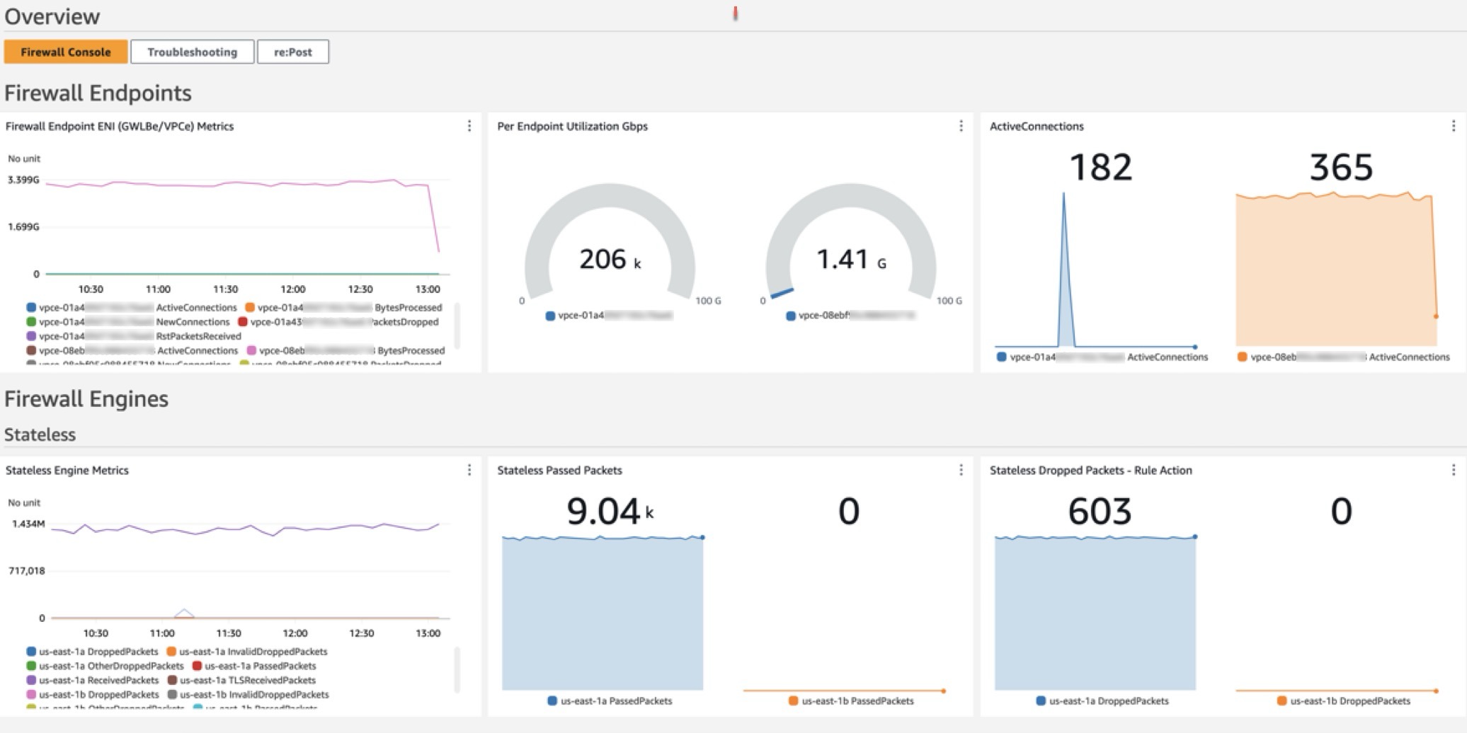
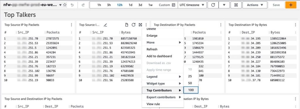
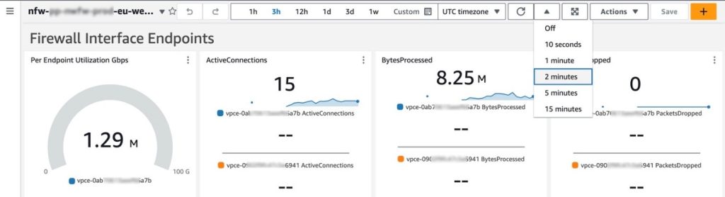
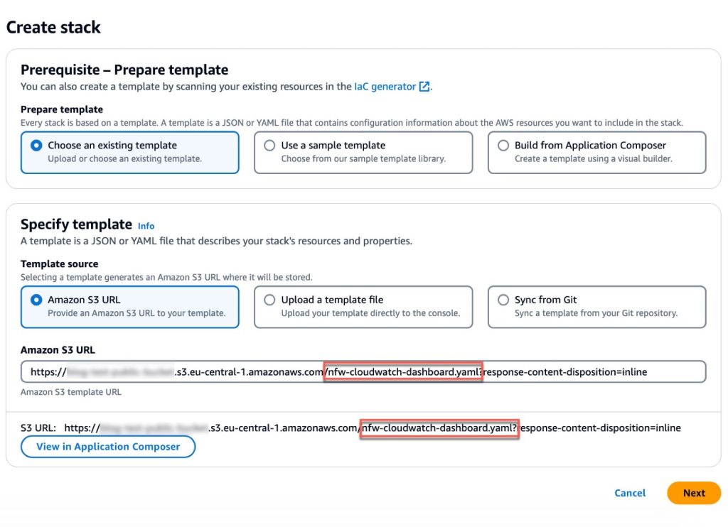


 Xu Feng is a Senior Industry Solution Architect at AWS, responsible for designing, building, and promoting industry solutions for the Media & Entertainment and Advertising sectors, such as intelligent customer service and business intelligence. With 20 years of software industry experience, currently focused on researching and implementing generative AI and AI-powered data solutions.
 Xu Da is a Amazon Web Services (AWS) Partner Solutions Architect based out of Shanghai, China. He has more than 25 years of experience in IT industry, software development and solution architecture. He is passionate about collaborative learning, knowledge sharing, and guiding community in their cloud technologies journey.


 Rohit Vashishtha is a Senior Analytics Specialist Solutions Architect at AWS based in Dallas, Texas. He has over 17 years of experience architecting, building, leading, and maintaining big data platforms. Rohit helps customers modernize their analytic workloads using the breadth of AWS services and ensures that customers get the best price/performance with utmost security and data governance.
 Jagadish Kumar (Jag) is a Senior Specialist Solutions Architect at AWS focused on Amazon OpenSearch Service. He is deeply passionate about Data Architecture and helps customers build analytics solutions at scale on AWS.
 Adam Gaulding is a Solution Architect at Satori. At Satori, Adam is helping customers implement data security controls on databases, data lakes and data warehouses. Adam has been in and around the data space throughout his 20+ year career. He’s worked with companies large and small and prides himself in building creative solutions for technical problems.