Post Syndicated from Danilo Poccia original https://aws.amazon.com/blogs/aws/introducing-amazon-neptune-serverless-a-fully-managed-graph-database-that-adjusts-capacity-for-your-workloads/
Amazon Neptune is a fully managed graph database service that makes it easy to build and run applications that work with highly connected datasets. With Neptune, you can use open and popular graph query languages to execute powerful queries that are easy to write and perform well on connected data. You can use Neptune for graph use cases such as recommendation engines, fraud detection, knowledge graphs, drug discovery, and network security.
Neptune has always been fully managed and handles time-consuming tasks such as provisioning, patching, backup, recovery, failure detection and repair. However, managing database capacity for optimal cost and performance requires you to monitor and reconfigure capacity as workload characteristics change. Also, many applications have variable or unpredictable workloads where the volume and complexity of database queries can change significantly. For example, a knowledge graph application for social media may see a sudden spike in queries due to sudden popularity.
Introducing Amazon Neptune Serverless
Today, we’re making that easier with the launch of Amazon Neptune Serverless. Neptune Serverless scales automatically as your queries and your workloads change, adjusting capacity in fine-grained increments to provide just the right amount of database resources that your application needs. In this way, you pay only for the capacity you use. You can use Neptune Serverless for development, test, and production workloads and optimize your database costs compared to provisioning for peak capacity.
With Neptune Serverless you can quickly and cost-effectively deploy graphs for your modern applications. You can start with a small graph, and as your workload grows, Neptune Serverless will automatically and seamlessly scale your graph databases to provide the performance you need. You no longer need to manage database capacity and you can now run graph applications without the risk of higher costs from over-provisioning or insufficient capacity from under-provisioning.
With Neptune Serverless, you can continue to use the same query languages (Apache TinkerPop Gremlin, openCypher, and RDF/SPARQL) and features (such as snapshots, streams, high availability, and database cloning) already available in Neptune.
Let’s see how this works in practice.
Creating an Amazon Neptune Serverless Database
In the Neptune console, I choose Databases in the navigation pane and then Create database. For Engine type, I select Serverless and enter my-database as the DB cluster identifier.

I can now configure the range of capacity, expressed in Neptune capacity units (NCUs), that Neptune Serverless can use based on my workload. I can now choose a template that will configure some of the next options for me. I choose the Production template that by default creates a read replica in a different Availability Zone. The Development and Testing template would optimize my costs by not having a read replica and giving access to DB instances that provide burstable capacity.

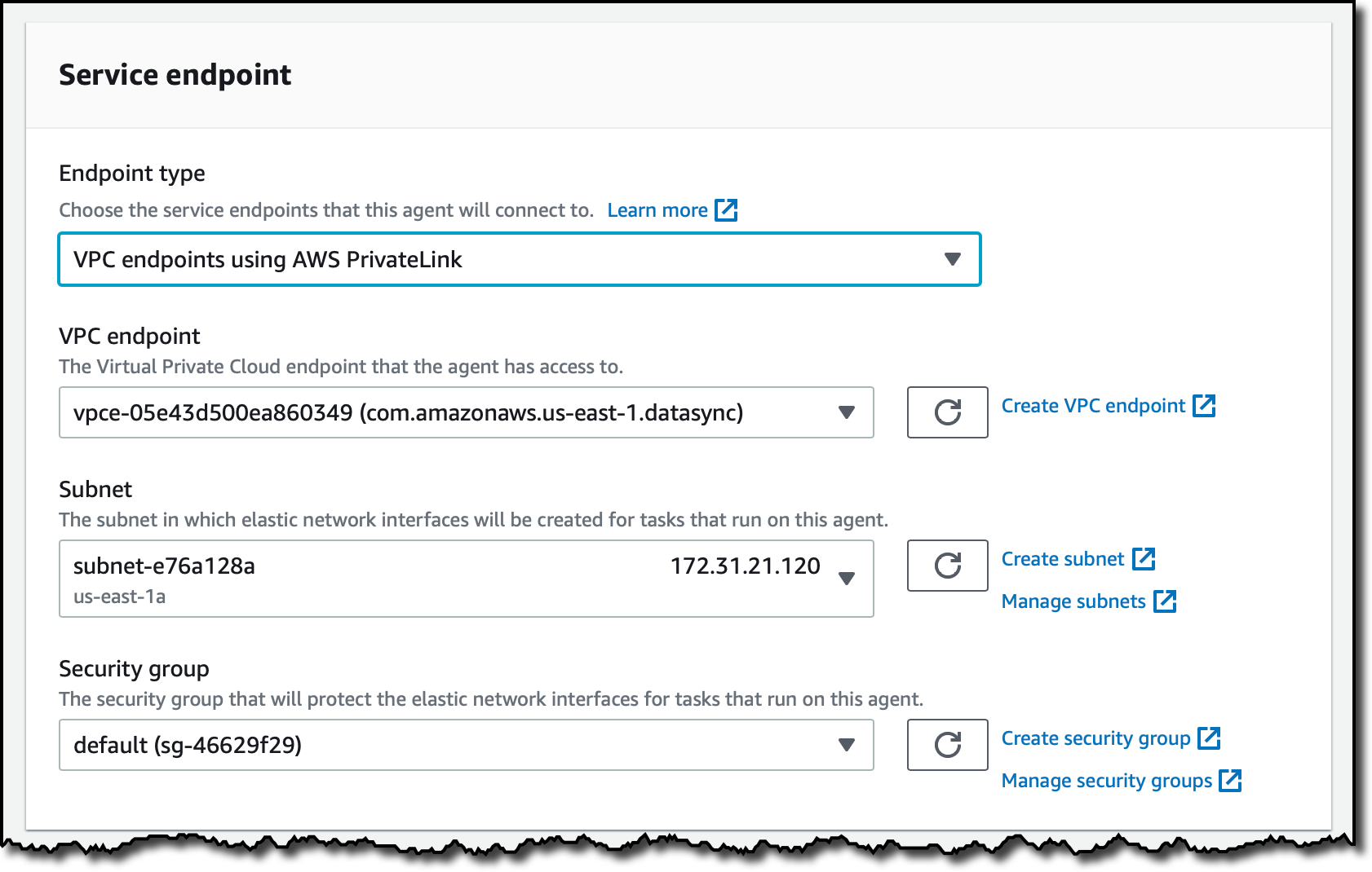
For Connectivity, I use my default VPC and its default security group.

Finally, I choose Create database. After a few minutes, the database is ready to use. In the list of databases, I choose the DB identifier to get the Writer and Reader endpoints that I am going to use later to access the database.
Using Amazon Neptune Serverless
There is no difference in the way you use Neptune Serverless compared to a provisioned Neptune database. I can use any of the query languages supported by Neptune. For this walkthrough, I choose to use openCypher, a declarative query language for property graphs originally developed by Neo4j that was open-sourced in 2015 and contributed to the openCypher project.
To connect to the database, I start an Amazon Linux Amazon Elastic Compute Cloud (Amazon EC2) instance in the same AWS Region and associate the default security group and a second security group that gives me SSH access.
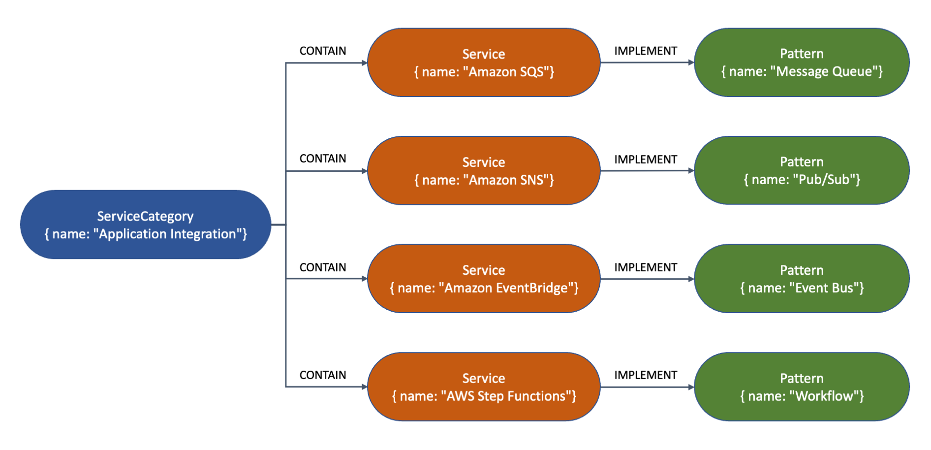
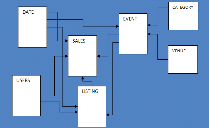
With a property graph I can represent connected data. In this case, I want to create a simple graph that shows how some AWS services are part of a service category and implement common enterprise integration patterns.
I use curl to access the Writer openCypher HTTPS endpoint and create a few nodes that represent patterns, services, and service categories. The following commands are split into multiple lines in order to improve readability.
This is a visual representation of the nodes and their relationships for the graph created by the previous command. The type (such as Service or Pattern) and properties (such as name) are shown inside each node. The arrows represent the relationships (such as CONTAIN or IMPLEMENT) between the nodes.
Now, I query the database to get some insights. To query the database, I can use either a Writer or a Reader endpoint. First, I want to know the name of the service implementing the “Message Queue” pattern. Note how the syntax of openCypher resembles that of SQL with MATCH instead of SELECT.
{
  "results" : [ {
    "s.name" : "Amazon SQS"
  } ]
}
I use the following query to see how many services are in the “Application Integration” category. This time, I use the WHERE clause to filter results.
{
  "results" : [ {
    "count(s)" : 4
  } ]
}
There are many options now that I have this graph database up and running. I can add more data (services, categories, patterns) and more relationships between the nodes. I can focus on my application and let Neptune Serverless manage capacity and infrastructure for me.
Availability and Pricing
Amazon Neptune Serverless is available today in the following AWS Regions: US East (Ohio, N. Virginia), US West (N. California, Oregon), Asia Pacific (Tokyo), and Europe (Ireland, London).
With Neptune Serverless, you only pay for what you use. The database capacity is adjusted to provide the right amount of resources you need in terms of Neptune capacity units (NCUs). Each NCU is a combination of approximately 2 gibibytes (GiB) of memory with corresponding CPU and networking. The use of NCUs is billed per second. For more information, see the Neptune pricing page.
Having a serverless graph database opens many new possibilities. To learn more, see the Neptune Serverless documentation. Let us know what you build with this new capability!
Simplify the way you work with highly connected data using Neptune Serverless.
— Danilo


 One-year anniversary of CloudFront Functions – I can’t believe it’s been