Post Syndicated from Danilo Poccia original https://aws.amazon.com/blogs/aws/new-move-payment-processing-to-the-cloud-with-aws-payment-cryptography/
Cryptography is everywhere in our daily lives. If you’re reading this blog, you’re using HTTPS, an extension of HTTP that uses encryption to secure communications. On AWS, multiple services and capabilities help you manage keys and encryption, such as:
- AWS Key Management Service (AWS KMS), which you can use to create and protect keys to encrypt or digitally sign your data.
- AWS CloudHSM, which you can use to manage single-tenant hardware security modules (HSMs).
HSMs are physical devices that securely protect cryptographic operations and the keys used by these operations. HSMs can help you meet your corporate, contractual, and regulatory compliance requirements. With CloudHSM, you have access to general-purpose HSMs. When payments are involved, there are specific payment HSMs that offer capabilities such as generating and validating the personal identification number (PIN) and the security code of a credit or debit card.
Today, I am happy to share the availability of AWS Payment Cryptography, an elastic service that manages payment HSMs and keys for payment processing applications in the cloud.
Applications using payments HSMs have challenging requirements because payment processing is complex, time sensitive, and highly regulated and requires the interaction of multiple financial service providers and payment networks. Every time you make a payment, data is exchanged between two or more financial service providers and must be decrypted, transformed, and encrypted again with a unique key at each step.
This process requires highly performant cryptography capabilities and key management procedures between each payment service provider. These providers might have thousands of keys to protect, manage, rotate, and audit, making the overall process expensive and difficult to scale. To add to that, payment HSMs historically employ complex and error-prone processes, such as exchanging keys in a secure room using multiple hand-carried paper forms, each with separate key components printed on them.
Introducing AWS Payment Cryptography
AWS Payment Cryptography simplifies your implementation of cryptographic functions and key management used to secure data in payment processing in accordance with various payment card industry (PCI) standards.
With AWS Payment Cryptography, you can eliminate the need to provision and manage on-premises payment HSMs and use the provided tools to avoid error-prone key exchange processes. For example, with AWS Payment Cryptography, payment and financial service providers can begin development within minutes and plan to exchange keys electronically, eliminating manual processes.
To provide its elastic cryptographic capabilities in a compliant manner, AWS Payment Cryptography uses HSMs with PCI PTS HSM device approval. These capabilities include encryption and decryption of card data, key creation, and pin translation. AWS Payment Cryptography is also designed in accordance with PCI security standards such as PCI DSS, PCI PIN, and PCI P2PE, and it provides evidence and reporting to help meet your compliance needs.
You can import and export symmetric keys between AWS Payment Cryptography and on-premises HSMs under key encryption key (KEKs) using the ANSI X9 TR-31 protocol. You can also import and export symmetric KEKs with other systems and devices using the ANSI X9 TR-34 protocol, which allows the service to exchange symmetric keys using asymmetric techniques.
To simplify moving consumer payment processing to the cloud, existing card payment applications can use AWS Payment Cryptography through the AWS SDKs. In this way, you can use your favorite programming language, such as Java or Python, instead of vendor-specific ASCII interfaces over TCP sockets, as is common with payment HSMs.
Access can be authorized using AWS Identity and Access Management (IAM) identity-based policies, where you can specify which actions and resources are allowed or denied and under which conditions.
Monitoring is important to maintain the reliability, availability, and performance needed by payment processing. With AWS Payment Cryptography, you can use Amazon CloudWatch, AWS CloudTrail, and Amazon EventBridge to understand what is happening, report when something is wrong, and take automatic actions when appropriate.
Let’s see how this works in practice.
Using AWS Payment Cryptography
Using the AWS Command Line Interface (AWS CLI), I create a double-length 3DES key to be used as a card verification key (CVK). A CVK is a key used for generating and verifying card security codes such as CVV, CVV2, and similar values.
Note that there are two commands for the CLI (and similarly two endpoints for API and SDKs):
payment-cryptographyfor control plane operation such as listing and creating keys and aliases.payment-cryptography-datafor cryptographic operations that use keys, for example, to generate PIN or card validation data.
Creating a key is a control plane operation:
{
    "Key": {
        "KeyArn": "arn:aws:payment-cryptography:us-west-2:123412341234:key/42cdc4ocf45mg54h",
        "KeyAttributes": {
            "KeyUsage": "TR31_C0_CARD_VERIFICATION_KEY",
            "KeyClass": "SYMMETRIC_KEY",
            "KeyAlgorithm": "TDES_2KEY",
            "KeyModesOfUse": {
                "Encrypt": false,
                "Decrypt": false,
                "Wrap": false,
                "Unwrap": false,
                "Generate": true,
                "Sign": false,
                "Verify": true,
                "DeriveKey": false,
                "NoRestrictions": false
            }
        },
        "KeyCheckValue": "B2DD4E",
        "KeyCheckValueAlgorithm": "ANSI_X9_24",
        "Enabled": true,
        "Exportable": false,
        "KeyState": "CREATE_COMPLETE",
        "KeyOrigin": "AWS_PAYMENT_CRYPTOGRAPHY",
        "CreateTimestamp": "2023-05-26T14:25:48.240000+01:00",
        "UsageStartTimestamp": "2023-05-26T14:25:48.220000+01:00"
    }
}
To reference this key in the next steps, I can use the Amazon Resource Name (ARN) as found in the KeyARN property, or I can create an alias. An alias is a friendly name that lets me refer to a key without having to use the full ARN. I can update an alias to refer to a different key. When I need to replace a key, I can just update the alias without having to change the configuration or the code of your applications. To be recognized easily, alias names start with alias/. For example, the following command creates the alias alias/my-key for the key I just created:
{
    "Alias": {
        "AliasName": "alias/my-key",
        "KeyArn": "arn:aws:payment-cryptography:us-west-2:123412341234:key/42cdc4ocf45mg54h"
    }
}
Before I start using the new key, I list all my keys to check their status:
{
    "Keys": [
        {
            "KeyArn": "arn:aws:payment-cryptography:us-west-2:123421341234:key/42cdc4ocf45mg54h",
            "KeyAttributes": {
                "KeyUsage": "TR31_C0_CARD_VERIFICATION_KEY",
                "KeyClass": "SYMMETRIC_KEY",
                "KeyAlgorithm": "TDES_2KEY",
                "KeyModesOfUse": {
                    "Encrypt": false,
                    "Decrypt": false,
                    "Wrap": false,
                    "Unwrap": false,
                    "Generate": true,
                    "Sign": false,
                    "Verify": true,
                    "DeriveKey": false,
                    "NoRestrictions": false
                }
            },
            "KeyCheckValue": "B2DD4E",
            "Enabled": true,
            "Exportable": false,
            "KeyState": "CREATE_COMPLETE"
        },
        {
            "KeyArn": "arn:aws:payment-cryptography:us-west-2:123412341234:key/ok4oliaxyxbjuibp",
            "KeyAttributes": {
                "KeyUsage": "TR31_C0_CARD_VERIFICATION_KEY",
                "KeyClass": "SYMMETRIC_KEY",
                "KeyAlgorithm": "TDES_2KEY",
                "KeyModesOfUse": {
                    "Encrypt": false,
                    "Decrypt": false,
                    "Wrap": false,
                    "Unwrap": false,
                    "Generate": true,
                    "Sign": false,
                    "Verify": true,
                    "DeriveKey": false,
                    "NoRestrictions": false
                }
            },
            "KeyCheckValue": "905848",
            "Enabled": true,
            "Exportable": false,
            "KeyState": "DELETE_PENDING"
        }
    ]
}
As you can see, there is another key I created before, which has since been deleted. When a key is deleted, it is marked for deletion (DELETE_PENDING). The actual deletion happens after a configurable period (by default, 7 days). This is a safety mechanism to prevent the accidental or malicious deletion of a key. Keys marked for deletion are not available for use but can be restored.
In a similar way, I list all my aliases to see to which keys they are they referring:
{
    "Aliases": [
        {
            "AliasName": "alias/my-key",
            "KeyArn": "arn:aws:payment-cryptography:us-west-2:123412341234:key/42cdc4ocf45mg54h"
        }
    ]
}
Now, I use the key to generate a card security code with the CVV2 authentication system. You might be familiar with CVV2 numbers that are usually written on the back of a credit card. This is the way they are computed. I provide as input the primary account number of the credit card, the card expiration date, and the key from the previous step. To specify the key, I use its alias. This is a data plane operation:
{
    "KeyArn": "arn:aws:payment-cryptography:us-west-2:123412341234:key/42cdc4ocf45mg54h",
    "KeyCheckValue": "B2DD4E",
    "ValidationData": "343"
}
I take note of the three digits in the ValidationData property. When processing a payment, I can verify that the card data value is correct:
{
    "KeyArn": "arn:aws:payment-cryptography:us-west-2:123412341234:key/42cdc4ocf45mg54h",
    "KeyCheckValue": "B2DD4E"
}
The verification is successful, and in return I get back the same KeyCheckValue as when I generated the validation data.
As you might expect, if I use the wrong validation data, the verification is not successful, and I get back an error:
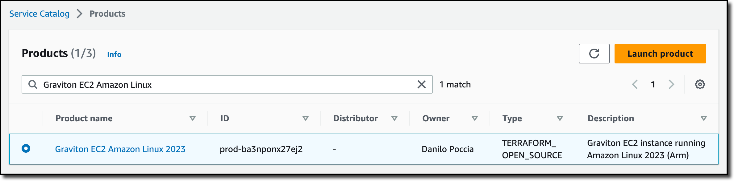
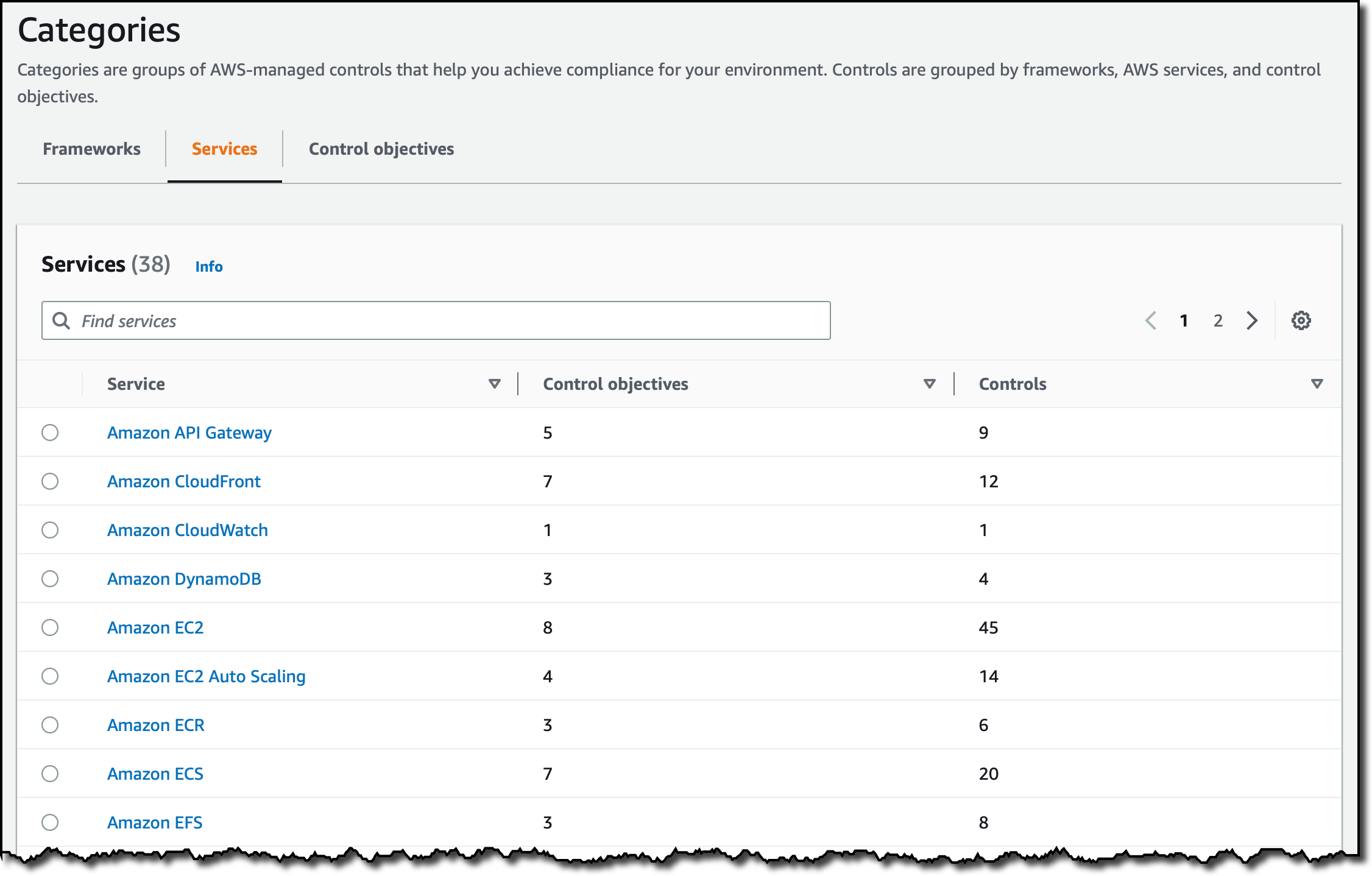
In the AWS Payment Cryptography console, I choose View Keys to see the list of keys.

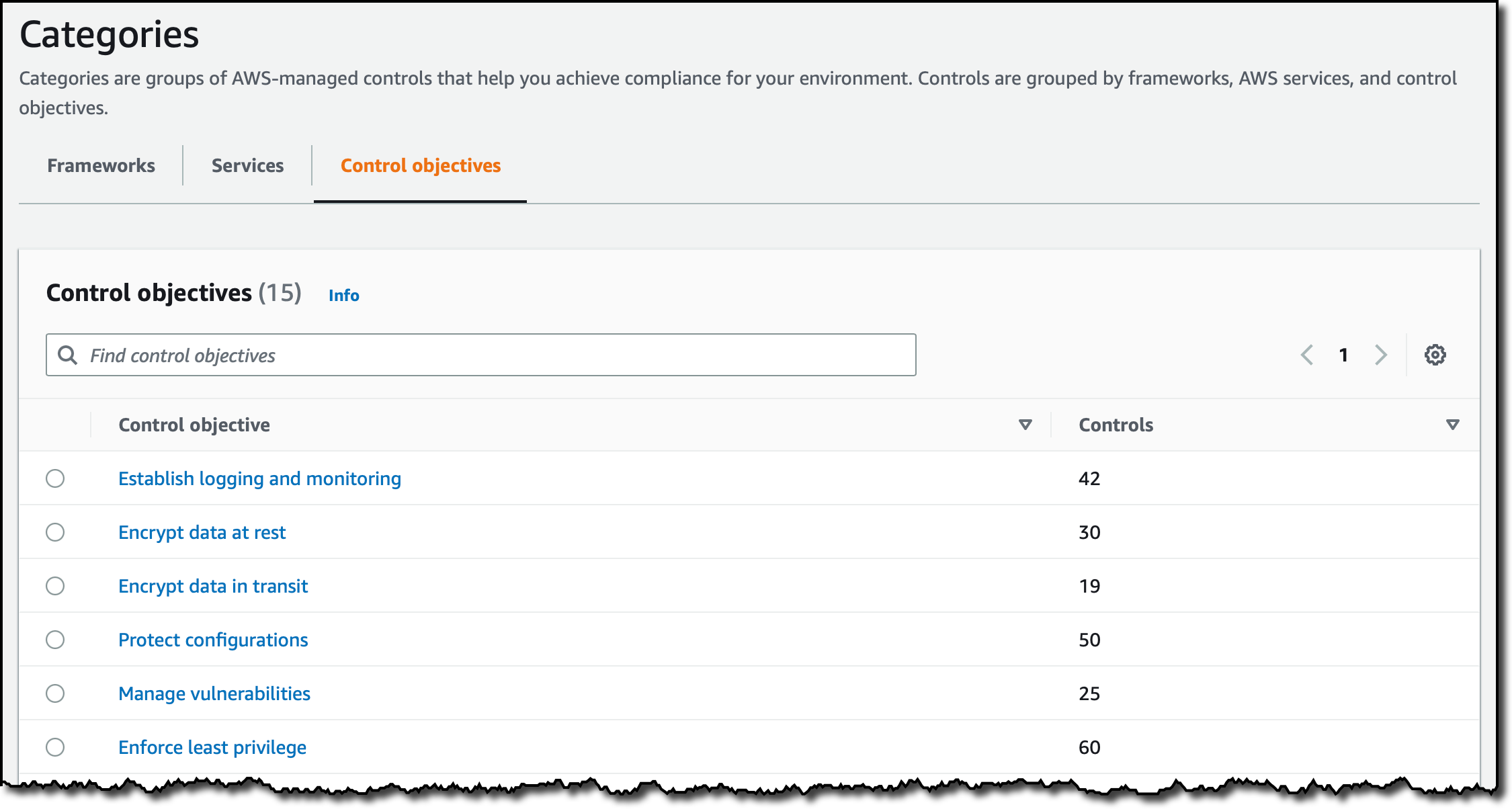
Optionally, I can enable more columns, for example, to see the key type (symmetric/asymmetric) and the algorithm used.

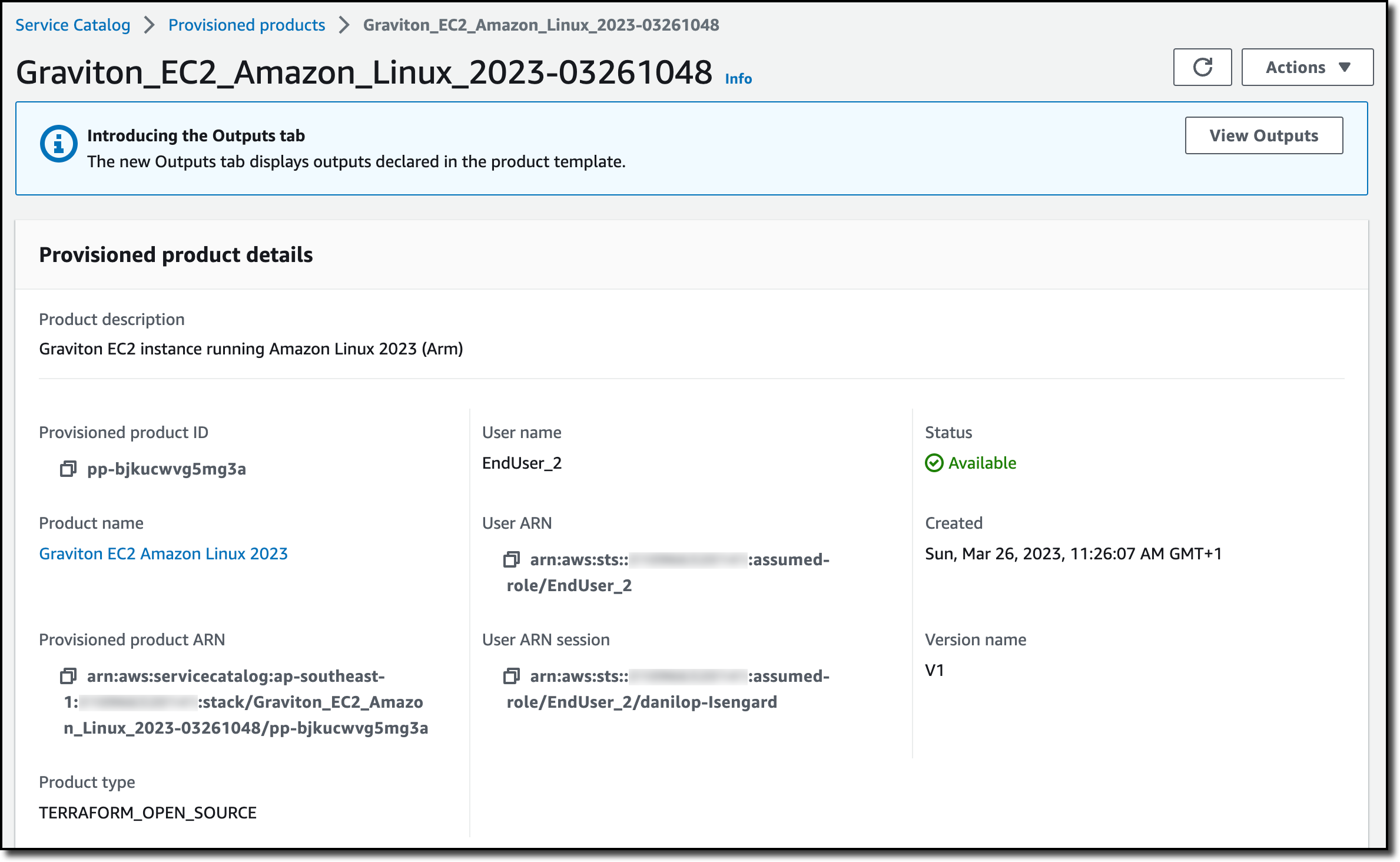
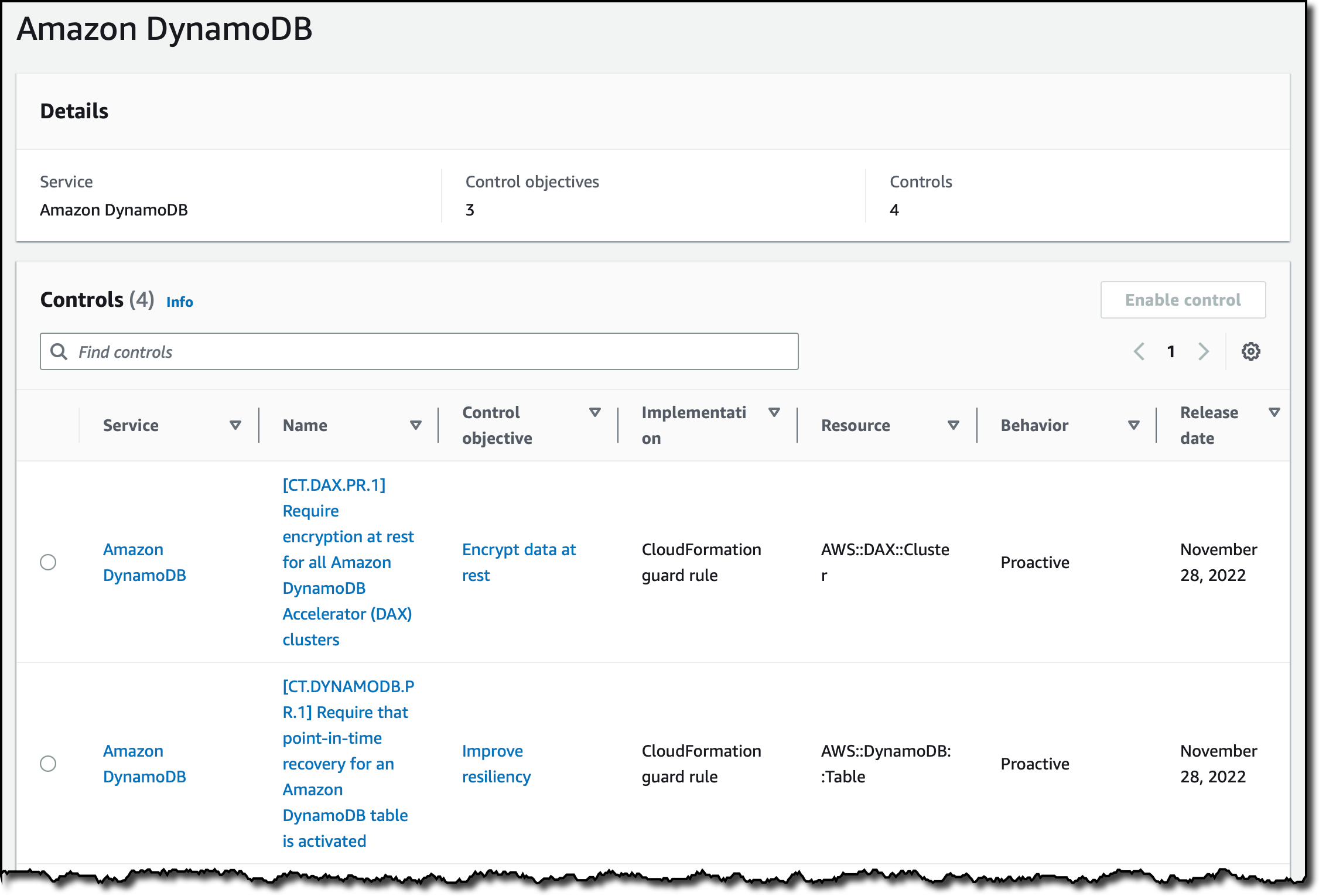
I choose the key I used in the previous example to get more details. Here, I see the cryptographic configuration, the tags assigned to the key, and the aliases that refer to this key.

AWS Payment Cryptography supports many more operations than the ones I showed here. For this walkthrough, I used the AWS CLI. In your applications, you can use AWS Payment Cryptography through any of the AWS SDKs.
Availability and Pricing
AWS Payment Cryptography is available today in the following AWS Regions: US East (N. Virginia) and US West (Oregon).
With AWS Payment Cryptography, you only pay for what you use based on the number of active keys and API calls with no up-front commitment or minimum fee. For more information, see AWS Payment Cryptography pricing.
AWS Payment Cryptography removes your dependencies on dedicated payment HSMs and legacy key management systems, simplifying your integration with AWS native APIs. In addition, by operating the entire payment application in the cloud, you can minimize round-trip communications and latency.
Move your payment processing applications to the cloud with AWS Payment Cryptography.
— Danilo