[$] The risks of embedded bare repositories in Git

Post Syndicated from original https://lwn.net/Articles/892755/

Running code from inside a cloned Git repository is potentially risky, but
normally just inspecting such a repository is considered to be safe. As a
recent posting to the Git mailing list shows, however, there are still
risks lurking inside these repositories; code that lives in them can be
triggered in unexpected ways. In particular, malicious “bare” repositories
can be added as a subdirectory of a repository; they can be configured to run
code whenever Git commands are executed there, which is something that can
happen in surprising ways. There is now an effort
underway to try to address the problem in Git, without breaking the
legitimate need for including bare repositories into a Git tree.

New – Storage-Optimized Amazon EC2 Instances (I4i) Powered by Intel Xeon Scalable (Ice Lake) Processors

Post Syndicated from Jeff Barr original https://aws.amazon.com/blogs/aws/new-storage-optimized-amazon-ec2-instances-i4i-powered-by-intel-xeon-scalable-ice-lake-processors/

Over the years we have released multiple generations of storage-optimized Amazon Elastic Compute Cloud (Amazon EC2) instances including the HS1 (2012) , D2 (2015), I2 (2013) , I3 (2017), I3en (2019), D3/D3en (2020), and Im4gn/Is4gen (2021). These instances are used to host high-performance real-time relational databases, distributed file systems, data warehouses, key-value stores, and more.

New I4i Instances
Today I am happy to introduce the new I4i instances, powered by the latest generation Intel Xeon Scalable (Ice Lake) Processors with an all-core turbo frequency of 3.5 GHz.

The instances offer up to 30 TB of NVMe storage using AWS Nitro SSD devices that are custom-built by AWS, and are designed to minimize latency and maximize transactions per second (TPS) on workloads that need very fast access to medium-sized datasets on local storage. This includes transactional databases such as MySQL, Oracle DB, and Microsoft SQL Server, as well as NoSQL databases: MongoDB, Couchbase, Aerospike, Redis, and the like. They are also an ideal fit for workloads that can benefit from very high compute performance per TB of storage such as data analytics and search engines.

Here are the specs:

Instance Name vCPUs
Memory (DDR4) Local NVMe Storage
(AWS Nitro SSD)
Sequential Read Throughput
(128 KB Blocks)
Bandwidth
EBS-Optimized
Network
i4i.large 2 16 GiB 468 GB 350 MB/s Up to 10 Gbps Up to 10 Gbps
i4i.xlarge 4 32 GiB 937 GB 700 MB/s Up to 10 Gbps Up to 10 Gbps
i4i.2xlarge 8 64 GiB 1,875 GB 1,400 MB/s Up to 10 Gbps Up to 12 Gbps
i4i.4xlarge 16 128 GiB 3,750 GB 2,800 MB/s Up to 10 Gbps Up to 25 Gbps
i4i.8xlarge 32 256 GiB 7,500 GB
(2 x 3,750 GB)
5,600 MB/s 10 Gbps 18.75 Gbps
i4i.16xlarge 64 512 GiB 15,000 GB
(4 x 3,750 GB)
11,200 MB/s 20 Gbps 37.5 Gbps
i4i.32xlarge 128 1024 GiB 30,000 GB
(8 x 3,750 GB)
22,400 MB/s 40 Gbps 75 Gbps

In comparison to the Xen-based I3 instances, the Nitro-powered I4i instances give you:

  • Up to 60% lower storage I/O latency, along with up to 75% lower storage I/O latency variability.
  • A new, larger instance size (i4i.32xlarge).
  • Up to 30% better compute price/performance.

The i4i.16xlarge and i4.32xlarge instances give you control over C-states, and the i4i.32xlarge instances support non-uniform memory access (NUMA). All of the instances support AVX-512, and use Intel Total Memory Encryption (TME) to deliver always-on memory encryption.

From Our Customers
AWS customers and AWS service teams have been putting these new instances to the test ahead of today’s launch. Here’s what they had to say:

Redis Enterprises powers mission-critical applications for over 8,000 organizations. According to Yiftach Shoolman (Co-Founder and CTO of Redis):

We are thrilled with the performance we are seeing from the Amazon EC2 I4i instances which use the new low latency AWS Nitro SSDs. Our testing shows I4i instances delivering an astonishing 2.9x higher query throughput than the previous generation I3 instances. We have also tested with various read and write mixes, and observed consistent and linearly scaling performance.

ScyllaDB is a high performance NoSQL database that can take advantage of high performance cloud computing instances.
Avi Kivity (Co-Founder and CTO of ScyllaDB) told us:


When we tested I4i instances, we observed up to 2.7x increase in throughput per vCPU compared to I3 instances for reads. With an even mix of reads and writes, we observed 2.2x higher throughput per vCPU, with a 40% reduction in average latency than I3 instances. We are excited for the incredible performance and value these new instances will enable for our customers going forward.

Amazon QuickSight is a business intelligence service. After testing,
Tracy Daugherty (General Manager, Amazon Quicksight) reported that:

I4i instances have demonstrated superior performance over previous generation I instances, with a 30% improvement across operations. We look forward to using I4i to further elevate performance for our customers.

Available Now

You can launch I4i instances today in the AWS US East (N. Virginia), US East (Ohio), US West (Oregon), and Europe (Ireland) Regions (with more to come) in On-Demand and Spot form. Savings Plans and Reserved Instances are available, as are Dedicated Instances and Dedicated Hosts.

In order to take advantage of the performance benefits of these new instances, be sure to use recent AMIs that include current ENA drivers and support for NVMe 1.4.

To learn more, visit the I4i instance home page.

Jeff;

Zero-Day Vulnerabilities Are on the Rise

Post Syndicated from Bruce Schneier original https://www.schneier.com/blog/archives/2022/04/zero-day-vulnerabilities-are-on-the-rise.html

Both Google and Mandiant are reporting a significant increase in the number of zero-day vulnerabilities reported in 2021.

Google:

2021 included the detection and disclosure of 58 in-the-wild 0-days, the most ever recorded since Project Zero began tracking in mid-2014. That’s more than double the previous maximum of 28 detected in 2015 and especially stark when you consider that there were only 25 detected in 2020. We’ve tracked publicly known in-the-wild 0-day exploits in this spreadsheet since mid-2014.

While we often talk about the number of 0-day exploits used in-the-wild, what we’re actually discussing is the number of 0-day exploits detected and disclosed as in-the-wild. And that leads into our first conclusion: we believe the large uptick in in-the-wild 0-days in 2021 is due to increased detection and disclosure of these 0-days, rather than simply increased usage of 0-day exploits.

Mandiant:

In 2021, Mandiant Threat Intelligence identified 80 zero-days exploited in the wild, which is more than double the previous record volume in 2019. State-sponsored groups continue to be the primary actors exploiting zero-day vulnerabilities, led by Chinese groups. The proportion of financially motivated actors­ — particularly ransomware groups — ­deploying zero-day exploits also grew significantly, and nearly 1 in 3 identified actors exploiting zero-days in 2021 was financially motivated. Threat actors exploited zero-days in Microsoft, Apple, and Google products most frequently, likely reflecting the popularity of these vendors. The vast increase in zero-day exploitation in 2021, as well as the diversification of actors using them, expands the risk portfolio for organizations in nearly every industry sector and geography, particularly those that rely on these popular systems.

News article.

How to control access to AWS resources based on AWS account, OU, or organization

Post Syndicated from Rishi Mehrotra original https://aws.amazon.com/blogs/security/how-to-control-access-to-aws-resources-based-on-aws-account-ou-or-organization/

AWS Identity and Access Management (IAM) recently launched new condition keys to make it simpler to control access to your resources along your Amazon Web Services (AWS) organizational boundaries. AWS recommends that you set up multiple accounts as your workloads grow, and you can use multiple AWS accounts to isolate workloads or applications that have specific security requirements. By using the new conditions, aws:ResourceOrgID, aws:ResourceOrgPaths, and aws:ResourceAccount, you can define access controls based on an AWS resource’s organization, organizational unit (OU), or account. These conditions make it simpler to require that your principals (users and roles) can only access resources inside a specific boundary within your organization. You can combine the new conditions with other IAM capabilities to restrict access to and from AWS accounts that are not part of your organization.

This post will help you get started using the new condition keys. We’ll show the details of the new condition keys and walk through a detailed example based on the following scenario. We’ll also provide references and links to help you learn more about how to establish access control perimeters around your AWS accounts.

Consider a common scenario where you would like to prevent principals in your AWS organization from adding objects to Amazon Simple Storage Service (Amazon S3) buckets that don’t belong to your organization. To accomplish this, you can configure an IAM policy to deny access to S3 actions unless aws:ResourceOrgID matches your unique AWS organization ID. Because the policy references your entire organization, rather than individual S3 resources, you have a convenient way to maintain this security posture across any number of resources you control. The new conditions give you the tools to create a security baseline for your IAM principals and help you prevent unintended access to resources in accounts that you don’t control. You can attach this policy to an IAM principal to apply this rule to a single user or role, or use service control policies (SCPs) in AWS Organizations to apply the rule broadly across your AWS accounts. IAM principals that are subject to this policy will only be able to perform S3 actions on buckets and objects within your organization, regardless of their other permissions granted through IAM policies or S3 bucket policies.

New condition key details

You can use the aws:ResourceOrgID, aws:ResourceOrgPaths, and aws:ResourceAccount condition keys in IAM policies to place controls on the resources that your principals can access. The following table explains the new condition keys and what values these keys can take.

Condition key Description Operator Single/multi value Value
aws:ResourceOrgID AWS organization ID of the resource being accessed All string operators Single value key Any AWS organization ID
aws:ResourceOrgPaths Organization path of the resource being accessed All string operators Multi-value key Organization paths of AWS organization IDs and organizational unit IDs
aws:ResourceAccount AWS account ID of the resource being accessed All string operators Single value key Any AWS account ID

Note: Of the three keys, only aws:ResourceOrgPaths is a multi-value condition key, while aws:ResourceAccount and aws:ResourceOrgID are single-value keys. For information on how to use multi-value keys, see Creating a condition with multiple keys or values in the IAM documentation.

Resource owner keys compared to principal owner keys

The new IAM condition keys complement the existing principal condition keys aws:PrincipalAccount, aws:PrincipalOrgPaths, and aws:PrincipalOrgID. The principal condition keys help you define which AWS accounts, organizational units (OUs), and organizations are allowed to access your resources. For more information on the principal conditions, see Use IAM to share your AWS resources with groups of AWS accounts in AWS Organizations on the AWS Security Blog.

Using the principal and resource keys together helps you establish permission guardrails around your AWS principals and resources, and makes it simpler to keep your data inside the organization boundaries you define as you continue to scale. For example, you can define identity-based policies that prevent your IAM principals from accessing resources outside your organization (by using the aws:ResourceOrgID condition). Next, you can define resource-based policies that prevent IAM principals outside your organization from accessing resources that are inside your organization boundary (by using the aws:PrincipalOrgID condition). The combination of both policies prevents any access to and from AWS accounts that are not part of your organization. In the next sections, we’ll walk through an example of how to configure the identity-based policy in your organization. For the resource-based policy, you can follow along with the example in An easier way to control access to AWS resources by using the AWS organization of IAM principals on the AWS Security blog.

Setup for the examples

In the following sections, we’ll show an example IAM policy for each of the new conditions. To follow along with Example 1, which uses aws:ResourceAccount, you’ll just need an AWS account.

To follow along with Examples 2 and 3 that use aws:ResourceOrgPaths and aws:ResourceOrgID respectively, you’ll need to have an organization in AWS Organizations and at least one OU created. This blog post assumes that you have some familiarity with the basic concepts in IAM and AWS Organizations. If you need help creating an organization or want to learn more about AWS Organizations, visit Getting Started with AWS Organizations in the AWS documentation.

Which IAM policy type should I use?

You can implement the following examples as identity-based policies, or in SCPs that are managed in AWS Organizations. If you want to establish a boundary for some of your IAM principals, we recommend that you use identity-based policies. If you want to establish a boundary for an entire AWS account or for your organization, we recommend that you use SCPs. Because SCPs apply to an entire AWS account, you should take care when you apply the following policies to your organization, and account for any exceptions to these rules that might be necessary for some AWS services to function properly.

Example 1: Restrict access to AWS resources within a specific AWS account

Let’s look at an example IAM policy that restricts access along the boundary of a single AWS account. For this example, say that you have an IAM principal in account 222222222222, and you want to prevent the principal from accessing S3 objects outside of this account. To create this effect, you could attach the following IAM policy.

{
  "Version": "2012-10-17",
  "Statement": [
    {
      "Sid": " DenyS3AccessOutsideMyBoundary",
      "Effect": "Deny",
      "Action": [
        "s3:*"
      ],
      "Resource": "*",
      "Condition": {
        "StringNotEquals": {
          "aws:ResourceAccount": [
            "222222222222"
          ]
        }
      }
    }
  ]
}

Note: This policy is not meant to replace your existing IAM access controls, because it does not grant any access. Instead, this policy can act as an additional guardrail for your other IAM permissions. You can use a policy like this to prevent your principals from access to any AWS accounts that you don’t know or control, regardless of the permissions granted through other IAM policies.

This policy uses a Deny effect to block access to S3 actions unless the S3 resource being accessed is in account 222222222222. This policy prevents S3 access to accounts outside of the boundary of a single AWS account. You can use a policy like this one to limit your IAM principals to access only the resources that are inside your trusted AWS accounts. To implement a policy like this example yourself, replace account ID 222222222222 in the policy with your own AWS account ID. For a policy you can apply to multiple accounts while still maintaining this restriction, you could alternatively replace the account ID with the aws:PrincipalAccount condition key, to require that the principal and resource must be in the same account (see example #3 in this post for more details how to accomplish this).

Organization setup: Welcome to AnyCompany

For the next two examples, we’ll use an example organization called AnyCompany that we created in AWS Organizations. You can create a similar organization to follow along directly with these examples, or adapt the sample policies to fit your own organization. Figure 1 shows the organization structure for AnyCompany.

Figure 1: Organization structure for AnyCompany

Figure 1: Organization structure for AnyCompany

Like all organizations, AnyCompany has an organization root. Under the root are three OUs: Media, Sports, and Governance. Under the Sports OU, there are three more OUs: Baseball, Basketball, and Football. AWS accounts in this organization are spread across all the OUs based on their business purpose. In total, there are six OUs in this organization.

Example 2: Restrict access to AWS resources within my organizational unit

Now that you’ve seen what the AnyCompany organization looks like, let’s walk through another example IAM policy that you can use to restrict access to a specific part of your organization. For this example, let’s say you want to restrict S3 object access within the following OUs in the AnyCompany organization:

  • Media
  • Sports
  • Baseball
  • Basketball
  • Football

To define a boundary around these OUs, you don’t need to list all of them in your IAM policy. Instead, you can use the organization structure to your advantage. The Baseball, Basketball, and Football OUs share a parent, the Sports OU. You can use the new aws:ResourceOrgPaths key to prevent access outside of the Media OU, the Sports OU, and any OUs under it. Here’s the IAM policy that achieves this effect.

{
  "Version": "2012-10-17",
  "Statement": [
    {
      "Sid": " DenyS3AccessOutsideMyBoundary",
      "Effect": "Deny",
      "Action": [
        "s3:*"
      ],
      "Resource": "*",
      "Condition": {
        "ForAllValues:StringNotLike": {
          "aws:ResourceOrgPaths": [
            "o-acorg/r-acroot/ou-acroot-mediaou/",
            "o-acorg/r-acroot/ou-acroot-sportsou/*"
          ] 
        }
      }
    }
  ]
}

Note: Like the earlier example, this policy does not grant any access. Instead, this policy provides a backstop for your other IAM permissions, preventing your principals from accessing S3 objects outside an OU-defined boundary. If you want to require that your IAM principals consistently follow this rule, we recommend that you apply this policy as an SCP. In this example, we attached this policy to the root of our organization, applying it to all principals across all accounts in the AnyCompany organization.

The policy denies access to S3 actions unless the S3 resource being accessed is in a specific set of OUs in the AnyCompany organization. This policy is identical to Example 1, except for the condition block: The condition requires that aws:ResourceOrgPaths contains any of the listed OU paths. Because aws:ResourceOrgPaths is a multi-value condition, the policy uses the ForAllValues:StringNotLike operator to compare the values of aws:ResourceOrgPaths to the list of OUs in the policy.

The first OU path in the list is for the Media OU. The second OU path is the Sports OU, but it also adds the wildcard character * to the end of the path. The wildcard * matches any combination of characters, and so this condition matches both the Sports OU and any other OU further down its path. Using wildcards in the OU path allows you to implicitly reference other OUs inside the Sports OU, without having to list them explicitly in the policy. For more information about wildcards, refer to Using wildcards in resource ARNs in the IAM documentation.

Example 3: Restrict access to AWS resources within my organization

Finally, we’ll look at a very simple example of a boundary that is defined at the level of an entire organization. This is the same use case as the preceding two examples (restrict access to S3 object access), but scoped to an organization instead of an account or collection of OUs.

{
  "Version": "2012-10-17",
  "Statement": [
    {
      "Sid": "DenyS3AccessOutsideMyBoundary",
      "Effect": "Deny",
      "Action": [
        "s3:*"
      ],
      "Resource": "arn:aws:s3:::*/*",
      "Condition": {
        "StringNotEquals": {
          "aws:ResourceOrgID": "${aws:PrincipalOrgID}"
        }
      }
    }
  ]
}

Note: Like the earlier examples, this policy does not grant any access. Instead, this policy provides a backstop for your other IAM permissions, preventing your principals from accessing S3 objects outside your organization regardless of their other access permissions. If you want to require that your IAM principals consistently follow this rule, we recommend that you apply this policy as an SCP. As in the previous example, we attached this policy to the root of our organization, applying it to all accounts in the AnyCompany organization.

The policy denies access to S3 actions unless the S3 resource being accessed is in the same organization as the IAM principal that is accessing it. This policy is identical to Example 1, except for the condition block: The condition requires that aws:ResourceOrgID and aws:PrincipalOrgID must be equal to each other. With this requirement, the principal making the request and the resource being accessed must be in the same organization. This policy also applies to S3 resources that are created after the policy is put into effect, so it is simple to maintain the same security posture across all your resources.

For more information about aws:PrincipalOrgID, refer to AWS global condition context keys in the IAM documentation.

Learn more

In this post, we explored the new conditions, and walked through a few examples to show you how to restrict access to S3 objects across the boundary of an account, OU, or organization. These tools work for more than just S3, though: You can use the new conditions to help you protect a wide variety of AWS services and actions. Here are a few links that you may want to look at:

If you have any questions, comments, or concerns, contact AWS Support or start a new thread on the AWS Identity and Access Management forum. Thanks for reading about this new feature. If you have feedback about this post, submit comments in the Comments section below.

Want more AWS Security news? Follow us on Twitter.

Rishi Mehrotra

Rishi Mehrotra

Rishi is a Product Manager in AWS IAM. He enjoys working with customers and influencing products decisions. Prior to Amazon, Rishi worked for enterprise IT customers after receiving engineering degree in computer science. He recently pursued MBA from The University of Chicago Booth School of Business. Outside of work, Rishi enjoys biking, reading, and playing with his kids.

Author

Michael Switzer

Mike is the product manager for the Identity and Access Management service at AWS. He enjoys working directly with customers to identify solutions to their challenges, and using data-driven decision making to drive his work. Outside of work, Mike is an avid cyclist and outdoorsperson. He holds a master’s degree in computational mathematics from the University of Washington.

Optimize AI/ML workloads for sustainability: Part 3, deployment and monitoring

Post Syndicated from Benoit de Chateauvieux original https://aws.amazon.com/blogs/architecture/optimize-ai-ml-workloads-for-sustainability-part-3-deployment-and-monitoring/

We’re celebrating Earth Day 2022 from 4/22 through 4/29 with posts that highlight how to build, maintain, and refine your workloads for sustainability.


AWS estimates that inference (the process of using a trained machine learning [ML] algorithm to make a prediction) makes up 90 percent of the cost of an ML model. Given with AWS you pay for what you use, we estimate that inference also generally equates to most of the resource usage within an ML lifecycle.

In this series, we’re following the phases of the Well-Architected machine learning lifecycle (Figure 1) to optimize your artificial intelligence (AI)/ML workloads. In Part 3, our final piece in the series, we show you how to reduce the environmental impact of your ML workload once your model is in production.


If you missed the first parts of this series, in Part 1, we showed you how to examine your workload to help you 1) evaluate the impact of your workload, 2) identify alternatives to training your own model, and 3) optimize data processing. In Part 2, we identified ways to reduce the environmental impact of developing, training, and tuning ML models.


ML lifecycle

Figure 1. ML lifecycle

Deployment

Select sustainable AWS Regions

As mentioned in Part 1, select an AWS Region with sustainable energy sources. When regulations and legal aspects allow, choose Regions near Amazon renewable energy projects and Regions where the grid has low published carbon intensity to deploy your model.

Align SLAs with sustainability goals

Define SLAs that support your sustainability goals while meeting your business requirements:

Use efficient silicon

For CPU-based ML inference, use AWS Graviton3. These processors offer the best performance per watt in Amazon Elastic Compute Cloud (Amazon EC2). They use up to 60% less energy than comparable EC2 instances. Graviton3 processors deliver up to three times better performance compared to Graviton2 processors for ML workloads, and they support bfloat16.

For deep learning workloads, the Amazon EC2 Inf1 instances (based on custom designed AWS Inferentia chips) deliver 2.3 times higher throughput and 80% lower cost compared to g4dn instances. Inf1 has 50% higher performance per watt than g4dn, which makes it the most sustainable ML accelerator Amazon EC2 offers.

Make efficient use of GPU

Use Amazon Elastic Inference to attach just the right amount of GPU-powered inference acceleration to any EC2 or SageMaker instance type or Amazon Elastic Container Service (Amazon ECS) task.

While training jobs batch process hundreds of data samples in parallel, inference jobs usually process a single input in real time, and thus consume a small amount of GPU compute. Elastic Inference allows you to reduce the cost and environmental impact of your inference by using GPU resources more efficiently.

Optimize models for inference

Improve efficiency of your models by compiling them into optimized forms with the following:

  • Various open-source libraries (like Treelite for decision tree ensembles)
  • Third-party tools like Hugging Face Infinity, which allows you to speed up transformer models and run inference not only on GPU but also on CPU.
  • SageMaker Neo’s runtime consumes as little as one-tenth the footprint of a deep learning framework and optimizes models to perform up to 25 time faster with no loss in accuracy (example with XGBoost).

Deploying more efficient models means you need fewer resources for inference.

Deploy multiple models behind a single endpoint

SageMaker provides three methods to deploy multiple models to a single endpoint to improve endpoint utilization:

  1. Host multiple models in one container behind one endpoint. Multi-model endpoints are served using a single container. This can help you cut up to 90 percent of your inference costs and carbon emissions.
  2. Host multiple models that use different containers behind one endpoint.
  3. Host a linear sequence of containers in an inference pipeline behind a single endpoint.

Sharing endpoint resources is more sustainable and less expensive than deploying a single model behind one endpoint.

Right-size your inference environment

Right-size your endpoints by using metrics from Amazon CloudWatch or by using the Amazon SageMaker Inference Recommender. This tool can run load testing jobs and recommend the proper instance type to host your model. When you use the appropriate instance type, you limit the carbon emission associated with over-provisioning.

If your workload has intermittent or unpredictable traffic, configure autoscaling inference endpoints in SageMaker to optimize your endpoints. Autoscaling monitors your endpoints and dynamically adjusts their capacity to maintain steady and predictable performance using as few resources as possible. You can also try Serverless Inference (in preview), which automatically launches compute resources and scales them in and out depending on traffic, which eliminates idle resources.

Consider inference at the edge

When working on Internet of Things (IoT) use cases, evaluate if ML inference at the edge can reduce the carbon footprint of your workload. To do this, consider factors like the compute capacity of your devices, their energy consumption, or the emissions related to data transfer to the cloud. When deploying ML models to edge devices, consider using SageMaker Edge Manager, which integrates with SageMaker Neo and AWS IoT Greengrass (Figure 2).

Run inference at the edge with SageMaker Edge

Figure 2. Run inference at the edge with SageMaker Edge

Device manufacturing represents 32-57 percent of the global Information Communication Technology carbon footprint. If your ML model is optimized, it requires less compute resources. You can then perform inference on lower specification machines, which minimizes the environmental impact of the device manufacturing and uses less energy.

The following techniques compress the size of models for deployment, which speeds up inference and saves energy without significant loss of accuracy:

  • Pruning removes weights (learnable parameters) that don’t contribute much to the model.
  • Quantization represents numbers with the low-bit integers without incurring significant loss in accuracy. Specifically, you can reduce resource usage by replacing the parameters in an inference model with half-precision (16 bit), bfloat16 (16 bit, but the same dynamic range as 32 bit), or 8-bit integers instead of the usual single-precision floating-point (32 bit) values.

Archive or delete unnecessary artifacts

Compress and reduce the volume of logs you keep during the inference phase. By default, CloudWatch retains logs indefinitely. By setting limited retention time for your inference logs, you’ll avoid the carbon footprint of unnecessary log storage. Also delete unused versions of your models and custom container images from your repositories.

Monitoring

Retrain only when necessary

Monitor your ML model in production and only retrain if it’s required. Because of model drift, robustness, or new ground truth data being available, models usually need to be retrained. Instead of retraining arbitrarily, monitor your ML model in production, automate your model drift detection and only retrain when your model’s predictive performance has fallen below defined KPIs.

Consider SageMaker PipelinesAWS Step Functions Data Science SDK for Amazon SageMaker, or third-party tools to automate your retraining pipelines.

Measure results and improve

To monitor and quantify improvements during the inference phase, track the following metrics:

For storage:

Conclusion

AI/ML workloads can be energy intensive, but as called out by UN and mentioned in the last IPCC report, AI can contribute to mitigation of climate change and the achievement of several Sustainable Development Goals. As technology builders, it’s our responsibility to make sustainable use of AI and ML.

In this blog post series, we presented best practices you can use to make sustainability-conscious architectural decisions and reduce the environmental impact for your AI/ML workloads.

Other posts in this series

About the Well-Architected Framework

These practices are part of the Sustainability Pillar of the AWS Well-Architected Framework. AWS Well-Architected is a set of guiding design principles developed by AWS to help organizations build secure, high-performing, resilient, and efficient infrastructure for a variety of applications and workloads. Use the AWS Well-Architected Tool to review your workloads periodically to address important design considerations and ensure that they follow the best practices and guidance of the AWS Well-Architected Framework. For follow up questions or comments, join our growing community on AWS re:Post.

Use a Cloudflare Worker to Send Notifications on Backblaze B2 Events

Post Syndicated from Pat Patterson original https://www.backblaze.com/blog/use-a-cloudflare-worker-to-send-notifications-on-backblaze-b2-events/

When building an application or solution on Backblaze B2 Cloud Storage, a common requirement is to be able to send a notification of an event (e.g., a user uploading a file) so that an application can take some action (e.g., processing the file). In this blog post, I’ll explain how you can use a Cloudflare Worker to send event notifications to a wide range of recipients, allowing great flexibility when building integrations with Backblaze B2.

Why Use a Proxy to Send Event Notifications?

Event notifications are useful whenever you need to ensure that a given event triggers a particular action. For example, last month, I explained how a video sharing site running on Vultr’s Infrastructure Cloud could store raw and transcoded videos in Backblaze B2. In that example, when a user uploaded a video to a Backblaze B2 bucket via the web application, the web app sent a notification to a Worker app instructing the Worker to read the raw video file from the bucket, transcode it, and upload the processed file back to Backblaze B2.

A drawback of this approach is that, if we were to create a mobile app to upload videos, we would have to copy the notification logic into the mobile app. As the system grows, so does the maintenance burden. Each new app needs code to send notifications and, worse, if we need to add a new field to the notification message, we have to update all of the apps. If, instead, we move the notification logic from the web application to a Cloudflare Worker, we can send notifications on Backblaze B2 events from a single location, regardless of the origin of the request. This pattern of wrapping an API with a component that presents the exact same API but adds its own functionality is known as a proxy.

Cloudflare Workers: A Brief Introduction

Cloudflare Workers provides a serverless execution environment that allows you to create applications that run on Cloudflare’s global edge network. A Cloudflare Worker application intercepts all HTTP requests destined for a given domain, and can return any valid HTTP response. Your Worker can create that HTTP response in any way you choose. Workers can consume a range of APIs, allowing them to directly interact with the Cloudflare cache, manipulate globally unique Durable Objects, perform cryptographic operations, and more.

Cloudflare Workers often, but not always, implement the proxy pattern, sending outgoing HTTP requests to servers on the public internet in the course of servicing incoming requests. If we implement a proxy that intercepts requests from clients to Backblaze B2, it could both forward those requests to Backblaze B2 and send notifications of those requests to one or more recipient applications.

This example focuses on proxying requests to the Backblaze S3 Compatible API, and can be used with any S3 client application that works with Backblaze B2 by simply changing the client’s endpoint configuration.

Implementing a similar proxy for the B2 Native API is much simpler, since B2 Native API requests are secured by a bearer token rather than a signature. A B2 Native API proxy would simply copy the incoming request, including the bearer token, changing only the target URL. Look out for a future blog post featuring a B2 Native API proxy.

Proxying Backblaze B2 Operations With a Cloudflare Worker

S3 clients send HTTP requests to the Backblaze S3 Compatible API over a TLS-secured connection. Each request includes the client’s Backblaze Application Key ID (access key ID in AWS parlance) and is signed with its Application Key (secret access key), allowing Backblaze B2 to authenticate the client and verify the integrity of the request. The signature algorithm, AWS Signature Version 4 (SigV4), includes the Host header in the signed data, ensuring that a request intended for one recipient cannot be redirected to another. Unfortunately, this is exactly what we want to happen in this use case!

Our proxy Worker must therefore validate the signature on the incoming request from the client, and then create a new signature that it can include in the outgoing request to the Backblaze B2 endpoint. Note that the Worker must be configured with the same Application Key and ID as the client to be able to validate and create signatures on the client’s behalf.

Here’s the message flow:

  1. A user performs an action in a Backblaze B2 client application, for example, uploading an image.
  2. The client app creates a signed request, exactly as it would for Backblaze B2, but sends it to the Cloudflare Worker rather than directly to Backblaze B2.
  3. The Worker validates the client’s signature, and creates its own signed request.
  4. The Worker sends the signed request to Backblaze B2.
  5. Backblaze B2 validates the signature, and processes the request.
  6. Backblaze B2 returns the response to the Worker.
  7. The Worker forwards the response to the client app.
  8. The Worker sends a notification to the webhook recipient.
  9. The recipient takes some action based on the notification.

These steps are illustrated in the diagram below.

The validation and signing process imposes minimal overhead, even for requests with large payloads, since the signed data includes a SHA-256 digest of the request payload, included with the request in the x-amz-content-sha256 HTTP header, rather than the payload itself. The Worker need not even read the incoming request payload into memory, instead passing it to the Cloudflare Fetch API to be streamed directly to the Backblaze B2 endpoint.

The Worker returns Backblaze B2’s response to the client unchanged, and creates a JSON-formatted webhook notification containing the following parameters:

  • contentLength: Size of the request body, if there was one, in bytes.
  • contentType: Describes the request body, if there was one. For example, image/jpeg.
  • method: HTTP method, for example, PUT.
  • signatureTimestamp: Request timestamp included in the signature.
  • status: HTTP status code returned from B2 Cloud Storage, for example 200 for a successful request or 404 for file not found.
  • url: The URL requested from B2 Cloud Storage, for example, https://s3.us-west-004.backblazeb2.com/my-bucket/hello.txt.

The Worker submits the notification to Cloudflare for asynchronous processing, so that the response to the client is not delayed. Once the interaction with the client is complete, Cloudflare POSTs the notification to the webhook recipient.

Prerequisites

If you’d like to follow the steps below to experiment with the proxy yourself, you will need to:

1. Creating a Cloudflare Worker Based on the Proxy Code

The Cloudflare Worker B2 Webhook GitHub repository contains full source code and configuration details. You can use the repository as a template for your own Worker using Cloudflare’s wrangler CLI. You can change the Worker name (my-proxy in the sample code below) as you see fit:

wrangler generate my-proxy
https://github.com/backblaze-b2-samples/cloudflare-b2-proxy
cd my-proxy

2. Configuring and Deploying the Cloudflare Worker

You must configure AWS_ACCESS_KEY_ID and AWS_S3_ENDPOINT in wrangler.toml before you can deploy the Worker. Configuring WEBHOOK_URL is optional—you can set it to empty quotes if you just want a vanity URL for Backblaze B2.

[vars]

AWS_ACCESS_KEY_ID = "<your b2 application key id>"
AWS_S3_ENDPOINT = "</your><your endpoint - e.g. s3.us-west-001.backblazeb2.com>"
AWS_SECRET_ACCESS_KEY = "Remove this line after you make AWS_SECRET_ACCESS_KEY a secret in the UI!"
WEBHOOK_URL = "<e.g. https://api.example.com/webhook/1 >"

Note the placeholder for AWS_SECRET_ACCESS_KEY in wrangler.toml. All variables used in the Worker must be set before the Worker can be published, but you should not save your Backblaze B2 application key to the file (see the note below). We work around these constraints by initializing AWS_SECRET_ACCESS_KEY with a placeholder value.

Use the CLI to publish the Worker project to the Cloudflare Workers environment:

wrangler publish

Now log in to the Cloudflare dashboard, navigate to your new Worker, and click the Settings tab, Variables, then Edit Variables. Remove the placeholder text, and paste your Backblaze B2 Application Key as the value for AWS_SECRET_ACCESS_KEY. Click the Encrypt button, then Save. The environment variables should look similar to this:

Finally, you must remove the placeholder line from wrangler.toml. If you do not do so, then the next time you publish the Worker, the placeholder value will overwrite your Application Key.

Why Not Just Set AWS_SECRET_ACCESS_KEY in wrangler.toml?

You should never, ever save secrets such as API keys and passwords in source code files. It’s too easy to forget to remove sensitive data from source code before sharing it either privately or, worse, on a public repository such as GitHub.

You can access the Worker via its default endpoint, which will have the form https://my-proxy.<your-workers-subdomain>.workers.dev, or create a DNS record in your own domain and configure a route associating the custom URL with the Worker.

If you try accessing the Worker URL via the browser, you’ll see an error message:

<Error>
<Code>AccessDenied</Code>
<Message>
Unauthenticated requests are not allowed for this api
</Message>
</Error>

This is expected—the Worker received the request, but the request did not contain a signature.

3. Configuring the Client Application

The only change required in your client application is the S3 endpoint configuration. Set it to your Cloudflare Worker’s endpoint rather than your Backblaze account’s S3 endpoint. As mentioned above, the client continues to use the same Application Key and ID as it did when directly accessing the Backblaze S3 Compatible API.

4. Implementing a Webhook Consumer

The webhook consumer must accept JSON-formatted messages via HTTP POSTs at a public endpoint accessible from the Cloudflare Workers environment. The webhook notification looks like this:

{
"contentLength": 30155,
"contentType": "image/png",
"method": "PUT",
"signatureTimestamp": "20220224T193204Z",
"status": 200,
"url": "https://s3.us-west-001.backblazeb2.com/my-bucket/image001.png"
}

You might implement the webhook consumer in your own application or, alternatively, use an integration platform such as IFTTT, Zapier, or Pipedream to trigger actions in downstream systems. I used Pipedream to create a workflow that logs each Backblaze B2 event as a new row in a Google Sheet. Watch it in action in this short video:

Put the Proxy to Work!

The Cloudflare Worker/Backblaze B2 Proxy can be used as-is in a wide variety of integrations—anywhere you need an event in Backblaze B2 to trigger an action elsewhere. At the same time, it can be readily adapted for different requirements. Here are a few ideas.

In this initial implementation, the client uses the same credentials to access the Worker as the Worker uses to access Backblaze B2. It would be straightforward to use different credentials for the upstream and downstream connections, ensuring that clients can’t bypass the Worker and access Backblaze B2 directly.

POSTing JSON data to a webhook endpoint is just one of many possibilities for sending notifications. You can integrate the worker with any system accessible from the Cloudflare Workers environment via HTTP. For example, you could use a stream-processing platform such as Apache Kafka to publish messages reliably to any number of consumers, or, similarly, send a message to an Amazon Simple Notification Service (SNS) topic for distribution to SNS subscribers.

As a final example, the proxy has full access to the request and response payloads. Rather than sending a notification to a separate system, the worker can operate directly on the data, for example, transparently compressing incoming uploads and decompressing downloads. The possibilities are endless.

How will you put the Cloudflare Worker Backblaze B2 Proxy to work? Sign up for a Backblaze B2 account and get started!

The post Use a Cloudflare Worker to Send Notifications on Backblaze B2 Events appeared first on Backblaze Blog | Cloud Storage & Cloud Backup.

Real-time analytics with Amazon Redshift streaming ingestion

Post Syndicated from Sam Selvan original https://aws.amazon.com/blogs/big-data/real-time-analytics-with-amazon-redshift-streaming-ingestion/

Amazon Redshift is a fast, scalable, secure, and fully managed cloud data warehouse that makes it simple and cost-effective to analyze all your data using standard SQL. Amazon Redshift offers up to three times better price performance than any other cloud data warehouse. Tens of thousands of customers use Amazon Redshift to process exabytes of data per day and power analytics workloads such as high-performance business intelligence (BI) reporting, dashboarding applications, data exploration, and real-time analytics.

We’re excited to launch Amazon Redshift streaming ingestion for Amazon Kinesis Data Streams, which enables you to ingest data directly from the Kinesis data stream without having to stage the data in Amazon Simple Storage Service (Amazon S3). Streaming ingestion allows you to achieve low latency in the order of seconds while ingesting hundreds of megabytes of data into your Amazon Redshift cluster.

In this post, we walk through the steps to create a Kinesis data stream, generate and load streaming data, create a materialized view, and query the stream to visualize the results. We also discuss the benefits of streaming ingestion and common use cases.

The need for streaming ingestion

We hear from our customers that you want to evolve your analytics from batch to real time, and access your streaming data in your data warehouses with low latency and high throughput. You also want to enrich your real-time analytics by combining them with other data sources in your data warehouse.

Use cases for Amazon Redshift streaming ingestion center around working with data that is generated continually (streamed) and needs to be processed within a short period (latency) of its generation. Sources of data can vary, from IoT devices to system telemetry, utility service usage, geolocation of devices, and more.

Before the launch of streaming ingestion, if you wanted to ingest real-time data from Kinesis Data Streams, you needed to stage your data in Amazon S3 and use the COPY command to load your data. This usually involved latency in the order of minutes and needed data pipelines on top of the data loaded from the stream. Now, you can ingest data directly from the data stream.

Solution overview

Amazon Redshift streaming ingestion allows you to connect to Kinesis Data Streams directly, without the latency and complexity associated with staging the data in Amazon S3 and loading it into the cluster. You can now connect to and access the data from the stream using SQL and simplify your data pipelines by creating materialized views directly on top of the stream. The materialized views can also include SQL transforms as part of your ELT (extract, load and transform) pipeline.

After you define the materialized views, you can refresh them to query the most recent stream data. This means that you can perform downstream processing and transformations of streaming data using SQL at no additional cost and use your existing BI and analytics tools for real-time analytics.

Amazon Redshift streaming ingestion works by acting as a stream consumer. A materialized view is the landing area for data that is consumed from the stream. When the materialized view is refreshed, Amazon Redshift compute nodes allocate each data shard to a compute slice. Each slice consumes data from the allocated shards until the materialized view attains parity with the stream. The very first refresh of the materialized view fetches data from the TRIM_HORIZON of the stream. Subsequent refreshes read data from the last SEQUENCE_NUMBER of the previous refresh until it reaches parity with the stream data. The following diagram illustrates this workflow.

Setting up streaming ingestion in Amazon Redshift is a two-step process. You first need to create an external schema to map to Kinesis Data Streams and then create a materialized view to pull data from the stream. The materialized view must be incrementally maintainable.

Create a Kinesis data stream

First, you need to create a Kinesis data stream to receive the streaming data.

  1. On the Amazon Kinesis console, choose Data streams.
  2. Choose Create data stream.
  3. For Data stream name, enter ev_stream_data.
  4. For Capacity mode, select On-demand.
  5. Provide the remaining configurations as needed to create your data stream.

Generate streaming data with the Kinesis Data Generator

You can synthetically generate data in JSON format using the Amazon Kinesis Data Generator (KDG) utility and the following template:

{
    
   "_id" : "{{random.uuid}}",
   "clusterID": "{{random.number(
        {   "min":1,
            "max":50
        }
    )}}", 
    "connectionTime": "{{date.now("YYYY-MM-DD HH:mm:ss")}}",
    "kWhDelivered": "{{commerce.price}}",
    "stationID": "{{random.number(
        {   "min":1,
            "max":467
        }
    )}}",
      "spaceID": "{{random.word}}-{{random.number(
        {   "min":1,
            "max":20
        }
    )}}",
 
   "timezone": "America/Los_Angeles",
   "userID": "{{random.number(
        {   "min":1000,
            "max":500000
        }
    )}}"
}

The following screenshot shows the template on the KDG console.

Load reference data

In the previous step, we showed you how to load synthetic data into the stream using the Kinesis Data Generator. In this section, you load reference data related to electric vehicle charging stations to the cluster.

Download the Plug-In EVerywhere Charging Station Network data from the City of Austin’s open data portal. Split the latitude and longitude values in the dataset and load it in to a table with the following schema.

CREATE TABLE ev_station
  (
     siteid                INTEGER,
     station_name          VARCHAR(100),
     address_1             VARCHAR(100),
     address_2             VARCHAR(100),
     city                  VARCHAR(100),
     state                 VARCHAR(100),
     postal_code           VARCHAR(100),
     no_of_ports           SMALLINT,
     pricing_policy        VARCHAR(100),
     usage_access          VARCHAR(100),
     category              VARCHAR(100),
     subcategory           VARCHAR(100),
     port_1_connector_type VARCHAR(100),
     voltage               VARCHAR(100),
     port_2_connector_type VARCHAR(100),
     latitude              DECIMAL(10, 6),
     longitude             DECIMAL(10, 6),
     pricing               VARCHAR(100),
     power_select          VARCHAR(100)
  ) DISTTYLE ALL

Create a materialized view

You can access your data from the data stream using SQL and simplify your data pipelines by creating materialized views directly on top of the stream. Complete the following steps:

  1. Create an external schema to map the data from Kinesis Data Streams to an Amazon Redshift object:
    CREATE EXTERNAL SCHEMA evdata FROM KINESIS
    IAM_ROLE 'arn:aws:iam::0123456789:role/redshift-streaming-role';

  2. Create an AWS Identity and Access Management (IAM) role (for the policy, see Getting started with streaming ingestion).

Now you can create a materialized view to consume the stream data. You can choose to use the SUPER datatype to store the payload as is in JSON format or use Amazon Redshift JSON functions to parse the JSON data into individual columns. For this post, we use the second method because the schema is well defined.

  1. Create the materialized view so it’s distributed on the UUID value from the stream and is sorted by the approximatearrivaltimestamp value:
    CREATE MATERIALIZED VIEW ev_station_data_extract DISTKEY(5) sortkey(1) AS
        SELECT approximatearrivaltimestamp,
        partitionkey,
        shardid,
        sequencenumber,
        json_extract_path_text(from_varbyte(data, 'utf-8'),'_id')::character(36) as ID,
        json_extract_path_text(from_varbyte(data, 'utf-8'),'clusterID')::varchar(30) as clusterID,
        json_extract_path_text(from_varbyte(data, 'utf-8'),'connectionTime')::varchar(20) as connectionTime,
        json_extract_path_text(from_varbyte(data, 'utf-8'),'kWhDelivered')::DECIMAL(10,2) as kWhDelivered,
        json_extract_path_text(from_varbyte(data, 'utf-8'),'stationID')::DECIMAL(10,2) as stationID,
        json_extract_path_text(from_varbyte(data, 'utf-8'),'spaceID')::varchar(100) as spaceID,
        json_extract_path_text(from_varbyte(data, 'utf-8'),'timezone')::varchar(30) as timezone,
        json_extract_path_text(from_varbyte(data, 'utf-8'),'userID')::varchar(30) as userID
        FROM evdata."ev_station_data";

  2. Refresh the materialized view:
    REFRESH MATERIALIZED VIEW ev_station_data_extract;

The materialized view doesn’t auto-refresh while in preview, so you should schedule a query in Amazon Redshift to refresh the materialized view once every minute. For instructions, refer to Scheduling SQL queries on your Amazon Redshift data warehouse.

Query the stream

You can now query the refreshed materialized view to get usage statistics:

SELECT to_timestamp(connectionTime, 'YYYY-MM-DD HH24:MI:SS') as connectiontime
,SUM(kWhDelivered) AS Energy_Consumed
,count(distinct userID) AS #Users
from ev_station_data_extract
group by to_timestamp(connectionTime, 'YYYY-MM-DD HH24:MI:SS')
order by 1 desc;

The following table contains the results.

connectiontime energy_consumed #users
2022-02-27 23:52:07+00 72870 131
2022-02-27 23:52:06+00 510892 998
2022-02-27 23:52:05+00 461994 934
2022-02-27 23:52:04+00 540855 1064
2022-02-27 23:52:03+00 494818 999
2022-02-27 23:52:02+00 491586 1000
2022-02-27 23:52:01+00 499261 1000
2022-02-27 23:52:00+00 774286 1498
2022-02-27 23:51:59+00 505428 1000
2022-02-27 23:51:58+00 262413 500
2022-02-27 23:51:57+00 486567 1000
2022-02-27 23:51:56+00 477892 995
2022-02-27 23:51:55+00 591004 1173
2022-02-27 23:51:54+00 422243 823
2022-02-27 23:51:53+00 521112 1028
2022-02-27 23:51:52+00 240679 469
2022-02-27 23:51:51+00 547464 1104
2022-02-27 23:51:50+00 495332 993
2022-02-27 23:51:49+00 444154 898
2022-02-27 23:51:24+00 505007 998
2022-02-27 23:51:23+00 499133 999
2022-02-27 23:29:14+00 497747 997
2022-02-27 23:29:13+00 750031 1496

Next, you can join the materialized view with the reference data to analyze the charging station consumption data for the last 5 minutes and break it down by station category:

SELECT to_timestamp(connectionTime, 'YYYY-MM-DD HH24:MI:SS') as connectiontime
,SUM(kWhDelivered) AS Energy_Consumed
,count(distinct userID) AS #Users
,st.category
from ev_station_data_extract ext
join ev_station st on
ext.stationID = st.siteid
where approximatearrivaltimestamp > current_timestamp -interval '5 minutes'
group by to_timestamp(connectionTime, 'YYYY-MM-DD HH24:MI:SS'),st.category
order by 1 desc, 2 desc

The following table contains the results.

connectiontime energy_consumed #users category
2022-02-27 23:55:34+00 188887 367 Workplace
2022-02-27 23:55:34+00 133424 261 Parking
2022-02-27 23:55:34+00 88446 195 Multifamily Commercial
2022-02-27 23:55:34+00 41082 81 Municipal
2022-02-27 23:55:34+00 13415 29 Education
2022-02-27 23:55:34+00 12917 24 Healthcare
2022-02-27 23:55:34+00 11147 19 Retail
2022-02-27 23:55:34+00 8281 14 Parks and Recreation
2022-02-27 23:55:34+00 5313 10 Hospitality
2022-02-27 23:54:45+00 146816 301 Workplace
2022-02-27 23:54:45+00 112381 216 Parking
2022-02-27 23:54:45+00 75727 144 Multifamily Commercial
2022-02-27 23:54:45+00 29604 55 Municipal
2022-02-27 23:54:45+00 13377 30 Education
2022-02-27 23:54:45+00 12069 26 Healthcare

Visualize the results

You can set up a simple visualization using Amazon QuickSight. For instructions, refer to Quick start: Create an Amazon QuickSight analysis with a single visual using sample data.

We create a dataset in QuickSight to join the materialized view with the charging station reference data.

Then, create a dashboard showing energy consumption and number of connected users over time. The dashboard also shows the list of locations on the map by category.

Streaming ingestion benefits

In this section, we discuss some of the benefits of streaming ingestion.

High throughput with low latency

Amazon Redshift can handle and process several gigabytes of data per second from Kinesis Data Streams. (Throughput is dependent on the number of shards in the data stream and the Amazon Redshift cluster configuration.) This allows you to experience low latency and high bandwidth when consuming streaming data, so you can derive insights from your data in seconds instead of minutes.

As we mentioned earlier, the key differentiator with the direct ingestion pull approach in Amazon Redshift is lower latency, which is in seconds. Contrast this to the approach of creating a process to consume the streaming data, staging the data in Amazon S3, and then running a COPY command to load the data into Amazon Redshift. This approach introduces latency in minutes due to the multiple steps involved in processing the data.

Straightforward setup

Getting started is easy. All the setup and configuration in Amazon Redshift uses SQL, which most cloud data warehouse users are already familiar with. You can get real-time insights in seconds without managing complex pipelines. Amazon Redshift with Kinesis Data Streams is fully managed, and you can run your streaming applications without requiring infrastructure management.

Increased productivity

You can perform rich analytics on streaming data within Amazon Redshift and using existing familiar SQL without needing to learn new skills or languages. You can create other materialized views, or views on materialized views, to do most of your ELT data pipeline transforms within Amazon Redshift using SQL.

Streaming ingestion use cases

With near-real time analytics on streaming data, many use cases and industry verticals applications become possible. The following are just some of the many application use cases:

  • Improve the gaming experience – You can focus on in-game conversions, player retention, and optimizing the gaming experience by analyzing real-time data from gamers.
  • Analyze clickstream user data for online advertising – The average customer visits dozens of websites in a single session, yet marketers typically analyze only their own websites. You can analyze authorized clickstream data ingested into the warehouse to assess your customer’s footprint and behavior, and target ads to your customers just-in-time.
  • Real-time retail analytics on streaming POS data – You can access and visualize all your global point of sale (POS) retail sales transaction data for real-time analytics, reporting, and visualization.
  • Deliver real-time application insights – With the ability to access and analyze streaming data from your application log files and network logs, developers and engineers can conduct real-time troubleshooting of issues, deliver better products, and alert systems for preventative measures.
  • Analyze IoT data in real time – You can use Amazon Redshift streaming ingestion with Amazon Kinesis services for real-time applications such as device status and attributes such as location and sensor data, application monitoring, fraud detection, and live leaderboards. You can ingest streaming data using Kinesis Data Streams, process it using Amazon Kinesis Data Analytics, and emit the results to any data store or application using Kinesis Data Streams with low end-to-end latency.

Conclusion

This post showed how to create Amazon Redshift materialized views to ingest data from Kinesis data streams using Amazon Redshift streaming ingestion. With this new feature, you can easily build and maintain data pipelines to ingest and analyze streaming data with low latency and high throughput.

The streaming ingestion preview is now available in all AWS Regions where Amazon Redshift is available. To get started with Amazon Redshift streaming ingestion, provision an Amazon Redshift cluster on the current track and verify your cluster is running version 1.0.35480 or later.

For more information, refer to Streaming ingestion (preview), and check out the demo Real-time Analytics with Amazon Redshift Streaming Ingestion on YouTube.


About the Author

Sam Selvan is a Senior Analytics Solution Architect with Amazon Web Services.

Amazon EMR on Amazon EKS provides up to 61% lower costs and up to 68% performance improvement for Spark workloads

Post Syndicated from Melody Yang original https://aws.amazon.com/blogs/big-data/amazon-emr-on-amazon-eks-provides-up-to-61-lower-costs-and-up-to-68-performance-improvement-for-spark-workloads/

Amazon EMR on Amazon EKS is a deployment option offered by Amazon EMR that enables you to run Apache Spark applications on Amazon Elastic Kubernetes Service (Amazon EKS) in a cost-effective manner. It uses the EMR runtime for Apache Spark to increase performance so that your jobs run faster and cost less.

Amazon EMR on Amazon EKS is a deployment option offered by Amazon EMR that enables you to run Apache Spark applications on Amazon Elastic Kubernetes Service (Amazon EKS) in a cost-effective manner. It uses the EMR runtime for Apache Spark to increase performance so that your jobs run faster and cost less.

In our benchmark tests using TPC-DS datasets at 3 TB scale, we observed that Amazon EMR on EKS provides up to 61% lower costs and up to 68% improved performance compared to running open-source Apache Spark on Amazon EKS via equivalent configurations. In this post, we walk through the performance test process, share the results, and discuss how to reproduce the benchmark. We also share a few techniques to optimize job performance that could lead to further cost-optimization for your Spark workloads.

How does Amazon EMR on EKS reduce cost and improve performance?

The EMR runtime for Spark is a performance-optimized runtime for Apache Spark that is 100% API compatible with open-source Apache Spark. It’s enabled by default with Amazon EMR on EKS. It helps run Spark workloads faster, leading to lower running costs. It includes multiple performance optimization features, such as Adaptive Query Execution (AQE), dynamic partition pruning, flattening scalar subqueries, bloom filter join, and more.

In addition to the cost benefit brought by the EMR runtime for Spark, Amazon EMR on EKS can take advantage of other AWS features to further optimize cost. For example, you can run Amazon EMR on EKS jobs on Amazon Elastic Compute Cloud (Amazon EC2) Spot Instances, providing up to 90% cost savings when compared to On-Demand Instances. Also, Amazon EMR on EKS supports Arm-based Graviton EC2 instances, which creates a 15% performance improvement and up to 30% cost savings when compared a Graviton2-based M6g to M5 instance type.

The recent graceful executor decommissioning feature makes Amazon EMR on EKS workloads more robust by enabling Spark to anticipate Spot Instance interruptions. Without the need to recompute or rerun impacted Spark jobs, Amazon EMR on EKS can further reduce job costs via critical stability and performance improvements.

Additionally, through container technology, Amazon EMR on EKS offers more options to debug and monitor Spark jobs. For example, you can choose Spark History Server, Amazon CloudWatch, or Amazon Managed Prometheus and Amazon Managed Grafana (for more details, refer to the Monitoring and Logging workshop). Optionally, you can use familiar command line tools such as kubectl to interact with a job processing environment and observe Spark jobs in real time, which provides a fail-fast and productive development experience.

Amazon EMR on EKS supports multi-tenant needs and offers application-level security control via a job execution role. It enables seamless integrations to other AWS native services without a key-pair set up in Amazon EKS. The simplified security design can reduce your engineering overhead and lower the risk of data breach. Furthermore, Amazon EMR on EKS handles security and performance patches so you can focus on building your applications.

Benchmarking

This post provides an end-to-end Spark benchmark solution so you can get hands-on with the performance test process. The solution uses unmodified TPC-DS data schema and table relationships, but derives queries from TPC-DS to support the Spark SQL test case. It is not comparable to other published TPC-DS benchmark results.

Key concepts

Transaction Processing Performance Council-Decision Support (TPC-DS) is a decision support benchmark that is used to evaluate the analytical performance of big data technologies. Our test data is a TPC-DS compliant dataset based on the TPC-DS Standard Specification, Revision 2.4 document, which outlines the business model and data schema, relationship, and more. As the whitepaper illustrates, the test data contains 7 fact tables and 17 dimension tables, with an average of 18 columns. The schema consists of essential retailer business information, such as customer, order, and item data for the classic sales channels: store, catalog, and internet. This source data is designed to represent real-world business scenarios with common data skews, such as seasonal sales and frequent names. Additionally, the TPC-DS benchmark offers a set of discrete scaling points (scale factors) based on the approximate size of the raw data. In our test, we chose the 3 TB scale factor, which produces 17.7 billion records, approximately 924 GB compressed data in Parquet file format.

Test approach

A single test session consists of 104 Spark SQL queries that were run sequentially. To get a fair comparison, each session of different deployment types, such as Amazon EMR on EKS, was run three times. The average runtime per query from these three iterations is what we analyze and discuss in this post. Most importantly, it derives two summarized metrics to represent our Spark performance:

  • Total execution time – The sum of the average runtime from three iterations
  • Geomean – The geometric mean of the average runtime
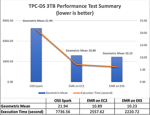
 Test results

In the test result summary (see the following figure), we discovered that the Amazon EMR-optimized Spark runtime used by Amazon EMR on EKS is approximately 2.1 times better than the open-source Spark on Amazon EKS in geometric mean and 3.5 times faster by the total runtime.

The following figure breaks down the performance summary by queries. We observed that EMR runtime for Spark was faster in every query compared to open-source Spark. Query q67 was the longest query in the performance test. The average runtime with open-source Spark was 1019.09 seconds. However, it took 150.02 seconds with Amazon EMR on EKS, which is 6.8 times faster. The highest performance gain in these long-running queries was q72—319.70 seconds (open-source Spark) vs. 26.86 seconds (Amazon EMR on EKS), a 11.9 times improvement.

Test cost

Amazon EMR pricing on Amazon EKS is calculated based on the vCPU and memory resources used from the time you start to download your EMR application Docker image until the Amazon EKS pod terminates. As a result, you don’t pay any Amazon EMR charges until your application starts to run, and you only pay for the vCPU and memory used during a job—you don’t pay for the full amount of compute resources in an EC2 instance.

Overall, the estimated benchmark cost in the US East (N. Virginia) Region is $22.37 per run for open-source Spark on Amazon EKS and $8.70 per run for Amazon EMR on EKS – that’s 61% cheaper due to the 68% quicker job runtime. The following table provides more details.

Benchmark Job Runtime (Hour) Estimated Cost Total EC2 Instance Total vCPU Total Memory (GiB) Root Device (EBS)
Amazon EMR on EKS 0.68 $8.70 6 216 432 20 GiB gp2
Open-Source Spark on Amazon EKS 2.13 $22.37 6 216 432 20 GiB gp2

Amazon EMR on Amazon EC2

(1 primary and 5 core nodes)

0.80 $8.80 6 196 424 20 GiB gp2

The cost estimate doesn’t account for Amazon Simple Storage Service (Amazon S3) storage, or PUT and GET requests. The Amazon EMR on EKS uplift calculation is based on the hourly billing information provided by AWS Cost Explorer.

Cost breakdown

The following is the cost breakdown for the Amazon EMR on EKS job ($8.70): 

  • Total uplift on vCPU – (126.93 * $0.01012) = (total number of vCPU used * per vCPU-hours rate) = $1.28
  • Total uplift on memory – (258.7 * $0.00111125) = (total amount of memory used * per GB-hours rate) = $0.29
  • Total Amazon EMR uplift cost – $1.57
  • Total Amazon EC2 cost – (6 * $1.728 * 0.68) = (number of instances * c5d.9xlarge hourly rate * job runtime in hour) = $7.05
  • Other costs – ($0.1 * 0.68) + ($0.1/730 * 20 * 6 * 0.68) = (shared Amazon EKS cluster charge per hour * job runtime in hour) + (EBS per GB-hourly rate * root EBS size * number of instances * job runtime in hour) = $0.08 

The following is the cost breakdown for the open-source Spark on Amazon EKS job ($22.37): 

  • Total Amazon EC2 cost – (6 * $1.728 * 2.13) = (number of instances * c5d.9xlarge hourly rate * job runtime in hour) = $22.12
  • Other costs – ($0.1 * 2.13) + ($0.1/730 * 20 * 6 * 2.13) = (shared EKS cluster charge per hour * job runtime in hour) + (EBS per GB-hourly rate * root EBS size * number of instances * job runtime in hour) = $0.25

The following is the cost breakdown for the Amazon EMR on Amazon EC2 ($8.80):

  • Total Amazon EMR cost – (5 * $0.27 * 0.80) + (1 * $0.192 * 0.80) = (number of core nodes * c5d.9xlarge Amazon EMR price * job runtime in hour) + (number of primary nodes * m5.4xlarge Amazon EMR price * job runtime in hour) = $1.23
  • Total Amazon EC2 cost – (5 * $1.728 * 0.80) + (1 * $0.768 * 0.80) = (number of core nodes * c5d.9xlarge instance price * job runtime in hour) + (number of primary nodes * m5.4xlarge instance price * job runtime in hour) = $7.53
  • Other Cost – ($0.1/730 * 20 GiB * 6 * 0.80) + ($0.1/730 * 256 GiB * 1 * 0.80) = (EBS per GB-hourly rate * root EBS size * number of instances * job runtime in hour) + (EBS per GB-hourly rate * default EBS size for m5.4xlarge * number of instances * job runtime in hour) = $0.041

Benchmarking considerations

In this section, we share some techniques and considerations for the benchmarking.

Set up an Amazon EKS cluster with Availability Zone awareness

Our Amazon EKS cluster configuration looks as follows:

apiVersion: eksctl.io/v1alpha5
kind: ClusterConfig
metadata:
  name: $EKSCLUSTER_NAME
  region: us-east-1
availabilityZones:["us-east-1a"," us-east-1b"]  
managedNodeGroups: 
  - name: mn-od
    availabilityZones: ["us-east-1b"] 

In the cluster configuration, the mn-od managed node group is assigned to the single Availability Zone b, where we run the test against.

Availability Zones are physically separated by a meaningful distance from other Availability Zones in the same AWS Region. This produces round trip latency between two compute instances located in different Availability Zones. Spark implements distributed computing, so exchanging data between compute nodes is inevitable when performing data joins, windowing, and aggregations across multiple executors. Shuffling data between multiple Availability Zones adds extra latency to the network I/O, which therefore directly impacts Spark performance. Additionally, when data is transferred between two Availability Zones, data transfer charges apply in both directions.

For this benchmark, which is a time-sensitive workload, we recommend running in a single Availability Zone and using On-Demand instances (not Spot) to have a dedicated compute resource. In an existing Amazon EKS cluster, you may have multiple instance types and a Multi-AZ setup. You can use the following Spark configuration to achieve the same goal:

--conf spark.kubernetes.node.selector.eks.amazonaws.com/capacityType=ON_DEMAND
--conf spark.kubernetes.node.selector.topology.kubernetes.io/zone=us-east-1b

Use instance store volume to increase disk I/O

Spark data shuffle, the process of reading and writing intermediate data to disk, is a costly operation. Besides the network I/O speed, Spark demands high performant disk to support a large amount of data redistribution activities. I/O operations per second (IOPS) is an equally important measure to baseline Spark performance. For instance, the SQL queries 23a, 23b, 50, and 93 are shuffle-intensive Spark workloads in TPC-DS, so choosing an optimal storage strategy can significantly shorten their runtime. General speaking, the recommended options are either attaching multiple EBS disk volumes per node in Amazon EKS or using the d series EC2 instance type, which offers high disk I/O performance within a compute family (for example, c5d.9xlarge is the d series in the c5 compute optimized family).

The following table summarizes the hardware specification we used:

Instance On-Demand Hourly Price vCPU Memory (GiB) Instance Store Networking Performance (Gbps) 100% Random Read IOPS Write IOPS
c5d.9xlarge $1.73 36 72 1 x 900GB NVMe SSD 10 350,000 170,000

To simplify our hardware configuration, we chose the AWS Nitro System EC2 instance type c5d.9xlarge, which comes with a NVMe-based SSD instance store volume. As of this writing, the built-in NVMe SSD disk requires less effort to set up and provides optimal disk performance we need. In the following code, the one-off preBoostrapCommand is triggered to mount an instance store to a node in Amazon EKS:

managedNodeGroups: 
  - name: mn-od
    preBootstrapCommands:
      - "sleep 5; sudo mkfs.xfs /dev/nvme1n1;sudo mkdir -p /local1;sudo echo /dev/nvme1n1 /local1 xfs defaults,noatime 1 2 >> /etc/fstab"
      - "sudo mount -a"
      - "sudo chown ec2-user:ec2-user /local1"

Run as a predefined job user, not a root user

For security, it’s not recommended to run Spark jobs as a root user. But how can you access the NVMe SSD volume mounted to the Amazon EKS cluster as a non-root Spark user?

An init container is created for each Spark driver and executor pods in order to set the volume permission and control the data access. Let’s check out the Spark driver pod via the kubectl exec command, which allows us execute into the running container and have an interactive session. We can observe the following:

  • The init container is called volume-permission.
  • The SSD disk is called /ossdata1. The Spark driver has stored some data to the disk.
  • The non-root Spark job user is called hadoop.

This configuration is provided in a format of a pod template file for Amazon EMR on EKS, so you can dynamically tailor job pods when Spark configuration doesn’t support your needs. Be aware that the predefined user’s UID in the EMR runtime for Spark is 999, but it’s set to 1000 in open-source Spark. The following is a sample Amazon EMR on EKS driver pod template:

apiVersion: v1
kind: Pod
spec:
  nodeSelector:
    app: sparktest
  volumes:
    - name: spark-local-dir-1
      hostPath:
        path: /local1  
  initContainers:  
  - name: volume-permission
    image: public.ecr.aws/y4g4v0z7/busybox
    # grant volume access to "hadoop" user with uid 999
    command: ['sh', '-c', 'mkdir /data1; chown -R 999:1000 /data1'] 
    volumeMounts:
      - name: spark-local-dir-1
        mountPath: /data1
  containers:
  - name: spark-kubernetes-driver
    volumeMounts:
      - name: spark-local-dir-1
        mountPath: /data1

In the job submission, we map the pod templates via the Spark configuration:

"spark.kubernetes.driver.podTemplateFile": "s3://'$S3BUCKET'/pod-template/driver-pod-template.yaml",
"spark.kubernetes.executor.podTemplateFile": "s3://'$S3BUCKET'/pod-template/executor-pod-template.yaml",

Spark on k8s operator is a popular tool to deploy Spark on Kubernetes. Our open-source Spark benchmark uses the tool to submit the job to Amazon EKS. However, the Spark operator currently doesn’t support file-based pod template customization, due to the way it operates. So we embed the disk permission setup into the job definition, as in the example on GitHub.

Disable dynamic resource allocation and enable Adaptive Query Execution in your application

Spark provides a mechanism to dynamically adjust compute resources based on workload. This feature is called dynamic resource allocation. It provides flexibility and efficiency to manage compute resources. For example, your application may give resources back to the cluster if they’re no longer used, and may request them again later when there is demand. It’s quite useful when your data traffic is unpredictable and an elastic compute strategy is needed at your application level. While running the benchmarking, our source data volume (3 TB) is certain and the jobs were run on a fixed-size Spark cluster that consists of six EC2 instances. You can turn off the dynamic allocation in EMR on EC2 as shown in the following code, because it doesn’t suit our purpose and might add latency to the test result. The rest of Spark deployment options, such as Amazon EMR on EKS, has the dynamic allocation off by default, so we can ignore these settings.

--conf spark.dynamicAllocation.enabled=false 
--conf spark.shuffle.service.enabled=false

Dynamic resource allocation is a different concept from automatic scaling in Amazon EKS, such as the Cluster Autoscaler. Disabling the dynamic allocation feature only fixes our 6-node Spark cluster size per job, but doesn’t stop the Amazon EKS cluster from expanding or shrinking automatically. It means our Amazon EKS cluster is still able to scale between 1 and 30 EC2 instances, as configured in the following code:

managedNodeGroups: 
  - name: mn-od
    availabilityZones: ["us-east-1b"] 
    instanceType: c5d.9xlarge
    minSize: 1
    desiredCapacity: 1
    maxSize: 30

Spark Adaptive Query Execution (AQE) is an optimization technique in Spark SQL since Spark 3.0. It dynamically re-optimizes the query execution plan at runtime, which supports a variety of optimizations, such as the following:

  • Dynamically switch join strategies
  • Dynamically coalesce shuffle partitions
  • Dynamically handle skew joins

The feature is enabled by default in EMR runtime for Spark, but disabled by default in open-source Apache Spark 3.1.2. To provide the fair comparison, make sure it’s set in the open-source Spark benchmark job declaration:

  sparkConf:
    # Enable AQE
    "spark.sql.adaptive.enabled": "true"
    "spark.sql.adaptive.localShuffleReader.enabled": "true"
    "spark.sql.adaptive.coalescePartitions.enabled": "true"
    "spark.sql.adaptive.skewJoin.enabled": "true"

Walkthrough overview

With these considerations in mind, we run three Spark jobs in Amazon EKS. This helps us compare Spark 3.1.2 performance in various deployment scenarios. For more details, check out the GitHub repository.

In this walkthrough, we show you how to do the following:

  • Produce a 3 TB TPC-DS complaint dataset
  • Run a benchmark job with the open-source Spark operator on Amazon EKS
  • Run the same benchmark application with Amazon EMR on EKS

We also provide information on how to benchmark with Amazon EMR on Amazon EC2.

Prerequisites

Install the following tools for the benchmark test:
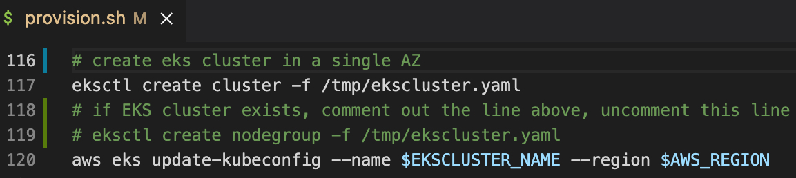
Provision resources

The provision script creates the following resources:

  • A new Amazon EKS cluster
  • Amazon EMR on EKS enabler
  • The required AWS Identity and Access Management (IAM) roles
  • The S3 bucket emr-on-eks-nvme-${ACCOUNTID}-${AWS_REGION}, referred to as <S3BUCKET> in the following steps

The provisioning process takes approximately 30 minutes.

  1. Download the project with the following command:
    git clone https://github.com/aws-samples/emr-on-eks-bencharmk.git
    cd emr-on-eks-bencharmk

  2. Create a test environment (change the Region if necessary):
    export EKSCLUSTER_NAME=eks-nvme
    export AWS_REGION=us-east-1
    
    ./provision.sh

Modify the script if needed for testing against an existing Amazon EKS cluster. Make sure the existing cluster has the Cluster Autoscaler and Spark Operator installed. Examples are provided by the script.

  1. Validate the setup:
    # should return results
    kubectl get pod -n oss | grep spark-operator
    kubectl get pod -n kube-system | grep nodescaler

Generate TPC-DS test data (optional)

In this optional task, you generate TPC-DS test data in s3://<S3BUCKET>/BLOG_TPCDS-TEST-3T-partitioned. The process takes approximately 80 minutes.

The job generates TPC-DS compliant datasets with your preferred scale. In this case, it creates 3 TB of source data (approximately 924 GB compressed) in Parquet format. We have pre-populated the source dataset in the S3 bucket blogpost-sparkoneks-us-east-1 in Region us-east-1. You can skip the data generation job if you want to have a quick start.

Be aware of that cross-Region data transfer latency will impact your benchmark result. It’s recommended to generate the source data to your S3 bucket if your test Region is different from us-east-1.

  1. Start the job:
    kubectl apply -f examples/tpcds-data-generation.yaml

  2. Monitor the job progress:
    kubectl get pod -n oss
    kubectl logs tpcds-data-generation-3t-driver -n oss

  3. Cancel the job if needed:
    kubectl delete -f examples/tpcds-data-generation.yaml

The job runs in the namespace oss with a service account called oss in Amazon EKS, which grants a minimum permission to access the S3 bucket via an IAM role. Update the example .yaml file if you have a different setup in Amazon EKS.

Benchmark for open-source Spark on Amazon EKS

Wait until the data generation job is complete, then update the default input location parameter (s3://blogpost-sparkoneks-us-east-1/blog/BLOG_TPCDS-TEST-3T-partitioned) to your S3 bucket in the tpcds-benchmark.yaml file.. Other parameters in the application can also be adjusted. Check out the comments in the yaml file for details. This process takes approximately 130 minutes.

If the data generation job is skipped, run the following steps without waiting.

  1. Start the job:
    kubectl apply -f examples/tpcds-benchmark.yaml

  2. Monitor the job progress:
    kubectl get pod -n oss
    kubectl logs tpcds-benchmark-oss-driver -n oss

  3. Cancel the job if needed:
    kubectl delete -f examples/tpcds-benchmark.yaml

The benchmark application outputs a CSV file capturing runtime per Spark SQL query and a JSON file with query execution plan details. You can use the collected metrics and execution plans to compare and analyze performance between different Spark runtimes (open-source Apache Spark vs. EMR runtime for Spark).

Benchmark with Amazon EMR on EKS

Wait for the data generation job finish before starting the benchmark for Amazon EMR on EKS. Don’t forget to change the input location (s3://blogpost-sparkoneks-us-east-1/blog/BLOG_TPCDS-TEST-3T-partitioned) to your S3 bucket. The output location is s3://<S3BUCKET>/EMRONEKS_TPCDS-TEST-3T-RESULT. If you use the pre-populated TPC-DS dataset, start the Amazon EMR on EKS benchmark without waiting. This process takes approximately 40 minutes.

  1. Start the job (change the Region if necessary):
    export EMRCLUSTER_NAME=emr-on-eks-nvme
    export AWS_REGION=us-east-1
    
    ./examples/emr6.5-benchmark.sh

Amazon EKS offers multi-tenant isolation and optimized resource allocation features, so it’s safe to run two benchmark tests in parallel on a single Amazon EKS cluster.

  1. Monitor the job progress in real time:
    kubectl get pod -n emr
    #run the command then search "execution time" in the log to analyze individual query's performance
    kubectl logs YOUR_DRIVER_POD_NAME -n emr spark-kubernetes-driver

  2. Cancel the job (get the IDs from the cluster list on the Amazon EMR console):
    aws emr-containers cancel-job-run --virtual-cluster-id <YOUR_VIRTUAL_CLUSTER_ID> --id <YOUR_JOB_ID>

The following are additional useful commands:

#Check volume status
kubectl exec -it YOUR_DRIVER_POD_NAME -c spark-kubernetes-driver -n emr -- df -h

#Login to a running driver pod
kubectl exec -it YOUR_DRIVER_POD_NAME -c spark-kubernetes-driver -n emr – bash

#Monitor compute resource usage
watch "kubectl top node"

Benchmark for Amazon EMR on Amazon EC2

Optionally, you can use the same benchmark solution to test Amazon EMR on Amazon EC2. Download the benchmark utility application JAR file from a running Kubernetes container, then submit a job via the Amazon EMR console. More details are available in the GitHub repository.

Clean up

To avoid incurring future charges, delete the resources generated if you don’t need the solution anymore. Run the following cleanup script (change the Region if necessary):

cd emr-on-eks-bencharmk

export EKSCLUSTER_NAME=eks-nvme
export AWS_REGION=us-east-1

./deprovision.sh

Conclusion

Without making any application changes, we can run Apache Spark workloads faster and cheaper with Amazon EMR on EKS when compared to Apache Spark on Amazon EKS. We used a benchmark solution running on a 6-node c5d.9xlarge Amazon EKS cluster and queried a TPC-DS dataset at 3 TB scale. The performance test result shows that Amazon EMR on EKS provides up to 61% lower costs and up to 68% performance improvement over open-source Spark 3.1.2 on Amazon EKS.

If you’re wondering how much performance gain you can achieve with your use case, try out the benchmark solution or the EMR on EKS Workshop. You can also contact your AWS Solution Architects, who can be of assistance alongside your innovation journey.


About the Authors

Melody Yang is a Senior Big Data Solution Architect for Amazon EMR at AWS. She is an experienced analytics leader working with AWS customers to provide best practice guidance and technical advice in order to assist their success in data transformation. Her areas of interests are open-source frameworks and automation, data engineering and DataOps.

Kinnar Kumar Sen is a Sr. Solutions Architect at Amazon Web Services (AWS) focusing on Flexible Compute. As a part of the EC2 Flexible Compute team, he works with customers to guide them to the most elastic and efficient compute options that are suitable for their workload running on AWS. Kinnar has more than 15 years of industry experience working in research, consultancy, engineering, and architecture.

[Security Nation] Whitney Merrill on the Crypto & Privacy Village (and the Latest in Data Privacy)

Post Syndicated from Rapid7 original https://blog.rapid7.com/2022/04/27/security-nation-whitney-merrill-on-the-crypto-privacy-village-and-the-latest-in-data-privacy/

[Security Nation] Whitney Merrill on the Crypto & Privacy Village (and the Latest in Data Privacy)

In this episode of Security Nation, Jen and Tod chat with Whitney Merrill, Data Protection Officer at Asana, about her work on the Crypto & Privacy Village and data privacy more broadly. She talks about how she keeps up with both the excitement and the effort of running the village, a mainstay at DEF CON each year – including the curveballs thrown by COVID-19. Whitney also takes Jen and Tod’s questions about the major data privacy topics of the day, touching on everything from vaccine passports to new legislation in California, targeted advertising, and the overlap between security and privacy.

Stick around for our Rapid Rundown, where Tod and Jen talk about psychic signatures in Java – which doesn’t involve ghosts, but does involve Dr. Who.

Whitney Merrill

[Security Nation] Whitney Merrill on the Crypto & Privacy Village (and the Latest in Data Privacy)

Whitney Merrill is Asana’s Data Protection Officer and heads up the growing privacy team. Previously she was Privacy, eCommerce & Consumer Protection Counsel at Electronic Arts (EA) and an attorney at the Federal Trade Commission. In her spare time, she runs the Crypto & Privacy Village, a nonprofit, which appears at DEF CON & BSidesSF each year.

Show notes

Interview links

Rapid Rundown links

Like the show? Want to keep Jen and Tod in the podcasting business? Feel free to rate and review with your favorite podcast purveyor, like Apple Podcasts.

Want More Inspiring Stories From the Security Community?

Subscribe to Security Nation Today

Cloudflare blocks 15M rps HTTPS DDoS attack

Post Syndicated from Omer Yoachimik original https://blog.cloudflare.com/15m-rps-ddos-attack/

Cloudflare blocks 15M rps HTTPS DDoS attack

Cloudflare blocks 15M rps HTTPS DDoS attack

Earlier this month, Cloudflare’s systems automatically detected and mitigated a 15.3 million request-per-second (rps) DDoS attack — one of the largest HTTPS DDoS attacks on record.

While this isn’t the largest application-layer attack we’ve seen, it is the largest we’ve seen over HTTPS. HTTPS DDoS attacks are more expensive in terms of required computational resources because of the higher cost of establishing a secure TLS encrypted connection. Therefore it costs the attacker more to launch the attack, and for the victim to mitigate it. We’ve seen very large attacks in the past over (unencrypted) HTTP, but this attack stands out because of the resources it required at its scale.

The attack, lasting less than 15 seconds, targeted a Cloudflare customer on the Professional (Pro) plan operating a crypto launchpad. Crypto launchpads are used to surface Decentralized Finance projects to potential investors. The attack was launched by a botnet that we’ve been observing — we’ve already seen large attacks as high as 10M rps matching the same attack fingerprint.

Cloudflare customers are protected against this botnet and do not need to take any action.

Cloudflare blocks 15M rps HTTPS DDoS attack

The attack

What’s interesting is that the attack mostly came from data centers. We’re seeing a big move from residential network Internet Service Providers (ISPs) to cloud compute ISPs.

This attack was launched from a botnet of approximately 6,000 unique bots. It originated from 112 countries around the world. Almost 15% of the attack traffic originated from Indonesia, followed by Russia, Brazil, India, Colombia, and the United States.

Cloudflare blocks 15M rps HTTPS DDoS attack

Within those countries, the attack originated from over 1,300 different networks. The top networks included the German provider Hetzner Online GmbH (Autonomous System Number 24940), Azteca Comunicaciones Colombia (ASN 262186), OVH in France (ASN 16276), as well as other cloud providers.

Cloudflare blocks 15M rps HTTPS DDoS attack

How this attack was automatically detected and mitigated

To defend organizations against DDoS attacks, we built and operate software-defined systems that run autonomously. They automatically detect and mitigate DDoS attacks across our entire network — and just as in this case, the attack was automatically detected and mitigated without any human intervention.

Our system starts by sampling traffic asynchronously; it then analyzes the samples and applies mitigations when needed.

Sampling

Initially, traffic is routed through the Internet via BGP Anycast to the nearest Cloudflare data centers that are located in over 250 cities around the world. Once the traffic reaches our data center, our DDoS systems sample it asynchronously allowing for out-of-path analysis of traffic without introducing latency penalties.

Analysis and mitigation

The analysis is done using data streaming algorithms. HTTP request samples are compared to conditional fingerprints, and multiple real-time signatures are created based on dynamic masking of various request fields and metadata. Each time another request matches one of the signatures, a counter is increased. When the activation threshold is reached for a given signature, a mitigation rule is compiled and pushed inline. The mitigation rule includes the real-time signature and the mitigation action, e.g. block.

Cloudflare customers can also customize the settings of the DDoS protection systems by tweaking the HTTP DDoS Managed Rules.

You can read more about our autonomous DDoS protection systems and how they work in our deep-dive technical blog post.

Helping build a better Internet

At Cloudflare, everything we do is guided by our mission to help build a better Internet. The DDoS team’s vision is derived from this mission: our goal is to make the impact of DDoS attacks a thing of the past. The level of protection that we offer is unmetered and unlimited — It is not bounded by the size of the attack, the number of the attacks, or the duration of the attacks. This is especially important these days because as we’ve recently seen, attacks are getting larger and more frequent.

Not using Cloudflare yet? Start now with our Free and Pro plans to protect your websites, or contact us for comprehensive DDoS protection for your entire network using Magic Transit.

Security updates for Wednesday

Post Syndicated from original https://lwn.net/Articles/892802/

Security updates have been issued by Mageia (virtualbox), Red Hat (container-tools:2.0, container-tools:3.0, gzip, kernel, kernel-rt, kpatch-patch, mariadb:10.3, mariadb:10.5, maven-shared-utils, polkit, vim, xmlrpc-c, and zlib), Scientific Linux (maven-shared-utils), SUSE (ant, go1.17, go1.18, kernel, and xen), and Ubuntu (fribidi, git, libcroco, libsepol, linux, linux-gcp, linux-ibm, linux-lowlatency, openjdk-17, and openjdk-lts).

Registering SMS Sender IDs in Singapore

Post Syndicated from Brent Meyer original https://aws.amazon.com/blogs/messaging-and-targeting/registering-sms-sender-ids-in-singapore/

A few weeks ago, we published a blog post about the process of registering alphanumeric Sender IDs. Today, we’re announcing support for registering Sender IDs in Singapore.

About Sender ID registration in Singapore

Singapore’s Infocomm Media Development Authority (IMDA) has created a Sender ID registry to protect consumers from fraudulent and malicious SMS messages. This registry is called the Singapore SMS Sender ID Registry (SSIR).

The government of Singapore encourages all government agencies and financial institutions to register with SSIR. Organizations and businesses outside of these industries can also register with SSIR.

Currently, there is no requirement to register your Sender ID. However, when you register with the SSIR, your Sender ID becomes a “Protected Sender ID.” Protected Sender IDs help to protect you and your customers by preventing other senders from using your Sender ID.

Note that in order to complete this registration process, your business or organization must have a Unique Entity Number (UEN). Businesses and other organizations receive a UEN when they register with Singapore’s Accounting and Corporate Regulatory Authority.

Registering your Sender ID

The first step in the registration process is to create a Protected Sender ID through the Singapore Network Information Centre (SGNIC). To initiate the registration process, send an email to [email protected]. In your message, include the name of your business, the Sender IDs that you want to register, and a description of your use case. SGNIC may contact you for additional information.

After you register with SGNIC, open a ticket in the AWS Support Center. You can find the procedure for opening a case in the Amazon Pinpoint User Guide. The AWS Support team will respond to your case within 24 hours. Their response includes a template for a letter that shows your intent to register a Sender ID.

The next step is to modify the contents of this letter. The regulatory groups in Singapore require a copy of this letter in order to allow AWS to send messages using your Sender ID. Begin by placing the contents of the letter on your company’s letterhead. Next, modify the fields that are highlighted in yellow. These fields include the following:

  • <Place>: The address of your company or organization.
  • <Brand Owner Company Name>: The name of your company or organization.
  • <Number>: Your Unique Entity Number.
  • <Signature>, <Name>, <Title>: The personal signature, name, and job title of the person who is submitting the request on behalf of your company or organization.
  • <ExampleSenderId1>, <ExampleSenderId2>: The Sender IDs that you intend to register with SGNIC. You can add or remove lines here depending on how many Sender IDs you plan to register.

Once you finish modifying the letter, submit it by attaching it to your existing case in the AWS Support Center.

What happens next?

IMDA regularly sends us lists of new Sender ID registrations. When we receive confirmation that your Sender ID has been registered, we update your account to allow it to send SMS messages through your Sender ID. We will also comment on your Support case to indicate that the process is complete.

Wrapping up

We continue to monitor changes to Sender ID registration requirements around the world. We’re working closely with carriers and organizations around the world to make the registration processes as straightforward as possible for our customers. Check in on this blog regularly to learn more about future regulatory changes.

For more information about registering Sender IDs in Singapore, see Special requirements for Singapore in the Amazon Pinpoint User Guide.

The collective thoughts of the interwebz